Error Control

for Molecular Statics Problems

Serge Prudhomme 1, Paul T. Bauman 2, and J. Tinsley Oden 3

Institute for Computational Engineering and Sciences

The University of Texas at Austin

Austin, Texas 78712

Abstract

In this paper, we present an extension of goal-oriented error estimation and adap-tation to the simulation of multi-scale problems of molecular statics. Computableerror estimates for the quasicontinuum method are developed with respect to spe-cific quantities of interest and an adaptive strategy based upon these estimates isproposed for error control. The theoretical results are illustrated on a nanoindenta-tion problem in which the quantity of interest is the force acting on the indenter.The promising capability of such error estimates and adaptive procedure for thesolution of multi-scale problems is demonstrated on numerical examples.

Key words: Molecular statics, goal-oriented adaptive modeling, error estimation,multi-scale problems, quasicontinuum method.

1 Introduction

Computational methods for the study of multi-scale phenomena have becomea prominent area of research in computational science. Indeed, computing ca-pabilities have reached a point where atomistic simulations using quantummechanical, atomistic potential, and mesoscopic and continuum models canbe coupled concurrently to study physical problems of an inherent multi-scalenature [2,8]. Development of such methods is of particular interest for the

Email address: serge@ices.utexas.edu (Serge Prudhomme).1 Corresponding author: Research Scientist, ICES.2 Graduate Research Assistant and DOE Fellow.3 Director of ICES and Cockrell Family Regents Chair of Engineering.

11 August 2005

study of the mechanics of materials including fracture phenomena, nanoin-dentation, atomic friction, etc., to name just a few [19,1]. However, many ofthe existing methods to date, to the best knowledge of the authors, lack someanalysis of the error incurred by coupling such models. Furthermore, conver-gence analysis and comparison studies of these methods seem to be scarce andnot fully addressed in the literature. In this paper, we present an applicationof goal-oriented error estimation and adaptive modeling to a model nanoin-dentation problem to partially address some of these issues. These ideas drawupon work in [11] where error estimates for quantities of interest are derived.Ideas of goal-oriented adaptive modeling come from [13] and references therein.This goal-oriented modeling methodology has been successfully applied to thestudy of heterogeneous elastostatics and elastodynamics, random heteroge-neous materials, as well as the study of linear lattice models [14,16,12]. Seealso [13].

In this study, an atomistic model based upon potentials of the embedded-atom method (EAM) is used as a base model to simulate the nanoindentationof a thin aluminum film [4,5]. The target problem was also studied in [19].Surrogate models are generated using the quasicontinuum method (QCM)[20,18]. Error estimates in a quantity of interest are derived and an adaptivemodeling scheme is implemented in the freely available QCM code [10]. A briefsummary of some of our results given in this paper were reported in the surveyarticle [13]. Here we give full details of an analysis of multi-scale modeling inwhich the coarse-scale modeling is implemented using the QCM.

The paper is organized as follows: following the introduction, we present inSection 2 the base model for molecular statics problems, derive a surrogatemodel based on the quasicontinuum method, and describe a practical examplethat deals with the nanoindentation of a thin film aluminum crystal. Section 3is devoted to the derivation of error estimates with respect to quantities of in-terest. These estimates approximate the modeling error between solutions ofthe base and surrogate models. In Section 4, an adaptive strategy is proposedfor the control of the modeling error by subsequent enrichment of the surrogatemodel. Performance of the error estimator and adaptive strategy is demon-strated on the nanoindentation problem described in Section 2. We finally givesome concluding remarks in Section 5.

2 Molecular statics model

In this section, we consider the problem of determining static equilibriumconfigurations of a regular lattice of N atoms. The base problem is obtainedby minimizing the potential energy of the system consisting of all atoms in

2

the lattice. In many applications, N can be very large and the base problemis often intractable. In order to reduce its complexity, we consider here theuse of an approximation method such as the quasicontinuum method (QCM)[18–20]. In recent years, QCM has become a popular approach for constructingsurrogate problems that retain only a small number of active atoms duringthe simulations. In that sense, QCM can be viewed as a model reductionprocedure.

2.1 The base problem. Let L be a regular lattice of N atoms in Rd, d = 2

or 3. The positions of the atoms are given in the reference configuration by thevectors xi ∈ R

d, i = 1, . . . , N . When the lattice is subjected to a deformationφ : R

d → Rd, the atoms move to the new positions

xi = φ(xi) = xi + ui, i = 1, . . . , N (1)

where ui is the displacement of atom i. We assume that the lattice in thereference configuration covers the region Ω, where Ω is an open bounded setof R

d with boundary ∂Ω. We also assume that the atoms lying on ∂Ω are allascribed essential boundary conditions in the form

ui = gi, ∀xi ∈ ∂Ω (2)

with gi ∈ Rd. Other boundary conditions will be considered in the nanoin-

dentation application. We deliberately choose to restrict ourselves to this casein the presentation of the theoretical results as, otherwise, it would make theexposition rather cumbersome without adding to the understanding of themethodology. Let Na be the number of atoms inside the domain Ω and Nb thenumber of atoms on ∂Ω such that N = Na + Nb. Henceforth, we shall use theconvention that the interior atoms be numbered from 1 to Na and the bound-ary atoms from Na + 1 to N . We will consider the finite-dimensional vectorspaces V = (Rd)N and V0 = (Rd)Na. In what follows, we will convenientlyuse the notation u = (u1, u2, . . . , uN ), u ∈ V , to refer to the displacementsof the collection of N atoms. Similarly, u ∈ V0 is the set of displacementsu = (u1, u2, . . . , uNa

).

Let a state of the system of N atoms be described by the displacements u ∈ V .The total potential energy of the system is assumed to take the form

E(u) = −N∑

i=1

f i · ui +N∑

k=1

Ek(u) (3)

where f i is the external load applied to an atom i and Ek(u) is the energyof atom k determined from inter-atomic potentials. Explicit description of Ek

will be given below.

3

The goal of molecular statics is to find the equilibrium state u ∈ V thatminimizes the total potential energy of the system, i.e.

E(u) = infv ∈ V

vi = gi on ∂Ω

E(v) (4)

The constrained minimization problem is then equivalent to finding u ∈ Vsuch that:

N∑

k=1

∂Ek

∂ui

(u) = f i, i = 1, . . . , Na (5)

ui = gi, i = Na + 1, . . . , N (6)

where ∂/∂ui is the gradient vector with respect to each component ul,i, l =1, . . . , d of the displacement vector ui, i.e. ∂/∂ui = (∂/∂u1,i, . . . , ∂/∂ud,i).

A variational formulation of the above problem is obtained by multiplying theNa equations in (5) by arbitrary vectors v ∈ V0 so that the problem reads

Find u ∈ V such that

B(u; v) = F (v), ∀v ∈ V0

ui = gi, i = Na + 1, . . . , N

(7)

where the semilinear form B(·; ·) and linear form F (·) are defined for anyu ∈ V and v ∈ V0 as

B(u; v) =Na∑

i=1

[

N∑

k=1

∂Ek

∂ui

(u)

]

· vi

F (v) =Na∑

i=1

f i · vi

(8)

Note that Problem (7) is nonlinear in u and linear in v. We assume that thereexist solutions and that it can be solved by a quasi-Newton method (see [17]for details).

2.2 The surrogate problem by the quasicontinuum method. We describe inthis section the main features of QCM. The reader is referred to [18,17,9]for a detailed exposition. The objectives of the method can be summarized asfollows: (i) to dramatically reduce the number of degrees of freedom from N×d,and (ii) to substantially reduce the cost in the calculation of the potentialenergy by computing energies only at selected sites. In addition, the use of

4

adaptive approaches for automatic selection of the degrees of freedom canallow QCM to capture the critical deformations of the lattice in an efficientmanner.

The initial step of the method consists in choosing a set of R N represen-tative atoms, the so-called “repatoms”, and in approximating u ∈ V by thereduced vector u0 ∈ W = (Rd)R. The displacements u0 represent the activedegrees of freedom of the system and the repatoms are conveniently identifiedwith the nodes of a finite element triangulation Ph of Ω. The displacements ofthe (N − R) “slave” atoms are then interpolated from u0 by piecewise linearpolynomials defined on the triangular mesh. Let φr, r = 1, . . . , R, denote thebasis functions (the hat functions) associated with Ph and let uh be the finiteelement vector function such that

uh(x) =R∑

r=1

u0,rφr(x), ∀x ∈ Ω (9)

u0 = (u0,1, u0,2, . . . , u0,R) ∈ W . The displacements of the N atoms in thelattice can clearly be evaluated from u0 as

u0i = uh(xi), i = 1, . . . , N (10)

so that u0 = (u01, u

02, . . . , u

0N) ∈ V . This extension operator will be referred

to as π : W → V such that πu0 = u0. In a similar manner, defining Ra andRb as the number of repatoms lying in the interior of the lattice and on theboundary ∂Ω, respectively, and letting W0 = (Rd)Ra, we also introduce theextension operator π0 : W0 → V0. The reduced vector πu0 could be used toapproximate the total potential energy

E(πu0) = −N∑

i=1

f i · (πu0)i +N∑

k=1

Ek(πu0) (11)

but such a calculation would still be very prohibitive as all N atoms need tobe visited in order to sum up the atomic site energies.

The second step of the QCM is thus concerned with and efficient scheme toapproximate the total energy E(πu0). The main motivation here is to estimatethe potential energy by summing only over the repatoms such that

E(πu0) ≈ E0(u0) = −R∑

r=1

nr f0,r · u0,r +R∑

r=1

nrEr(u0) (12)

where nr is an appropriate weight function associated with repatom r so as toaccount for all atoms in the lattice, i.e.

∑

r nr = N , and f0,r is the averaged

5

external force acting on repatom r. In the QCM, the calculation of the energiesnrEr(u0) is done in one of two ways, depending upon whether a repatom isconsidered either “local” or “nonlocal”. The attribute “local” refers here to thefact that the energy at a point in the continuum depends on the deformationat that point only and not on its surroundings. Let Rlc denote the numberof local repatoms and Rnl the number of nonlocal repatoms, R = Rlc + Rnl.The atomistic energies are now separated into local and nonlocal contributionssuch as:

R∑

r=1

nrEr(u0) =Rlc∑

r=1

nrEloc

r (u0) +Rnl∑

s=1

nsEnl

s (u0) (13)

Note that if Rnl = 0, the method is called the local QCM, and if Rlc =0, the nonlocal QCM. Otherwise, the method is referred to as the coupledlocal/nonlocal QCM. We shall only consider the latter in what follows.

Local formulation: The local formulation makes use of the Cauchy-Born rule [7]to compute the sites energies. The Cauchy-Born rule postulates that when acrystal is subjected to a small linear displacement of its boundary, then allinterior atoms are deformed following this displacement. In particular, thismeans that every atom in a region experiencing a uniform deformation gradi-ent has the same energy. Since the QCM uses piecewise linear finite elements,the deformation gradient is uniform within each element and the energy in anelement can be calculated by computing the energy of one atom only in thedeformed state. Then the energy E loc

r is given by:

nrEloc

r (u0) =K∑

e=1

ner E(F e), nr =

K∑

e=1

ner (14)

where E(F e) is the energy of a single atom under the deformation gradientF e. Here K is the number of elements surrounding the repatom r and ne

r isthe number of atoms from nr that actually live in element e.

Nonlocal formulation: In this formulation, the energy is accurately approx-imated by explicitly computing the energy of the nonlocal repatoms, i.e.Enl

s (u0) = Es(u0). In other words, if Rlc = 0 and in the limit case whereevery atom in the lattice is made a repatom, that is Rnl = N , then nr = 1,r = 1, . . . , N , and the problem becomes equivalent to the base problem.

Remark 1 (Ghost forces) The coupling of nonlocal and local representativeatoms leads to spurious forces, so-called “ghost forces”, near interfaces of localand nonlocal repatoms. The issue is that the energy calculated at a nonlocalrepatom may be influenced by the displacement of a local repatom nearby, whilethe converse may not be true. Therefore the approximation of the energy bythe coupled local/nonlocal approach yields non-physical forces at the interface

6

of the local and nonlocal regions. A solution to this issue has been devised byadding corrective forces to balance ghost forces (see e.g. [17]).

Remark 2 (Local/nonlocal criterion) The selection of representative at-oms as local or nonlocal is based upon the variation of the deformation gradienton the atomic scale in the vicinity of the atoms. A repatom is made local if thedeformation is almost uniform, nonlocal if the deformation gradient is large.In the QCM, the deformation gradients are compared element to element bycomputing the differences between the eigenvalues of the right stretch tensor

U =√

F T F in each element, F = ∇φ being the deformation gradient in theelements.

Using the approximation (12) for the potential energy, the minimization prob-lem for the QCM consists of finding u0 ∈ W such that

E0(u0) = minv ∈ W

vi = gi on ∂Ω

E0(v) (15)

This can be rewritten in variational form as

Find u0 ∈ W such that

B0(u0; v) = F0(v), ∀v ∈ W0

u0,i = gi, i = Ra + 1, . . . , R

(16)

where the semilinear form B0(·; ·) and linear form F0(·) are now given by

B0(u; v) =Ra∑

i=1

[

R∑

r=1

nr

∂Er

∂ui

(u)

]

· vi

F0(v) =Ra∑

i=1

ni f0,i · vi

(17)

Remark 3 (Adaptivity) In [9], it is proposed that an automatic mesh adap-tion technique be used to add and remove representative atoms “on the fly”,in order to capture the fine features during the simulation. The criterion foradaptivity is based upon the derivation of an error indicator similar to that ofZienkiewicz and Zhu [21] for the finite element method. The error indicator iscalculated over each element Ωe as

ηK =

√

1

|ΩK|∫

ΩK

(F − F ) : (F − F )dx

where |ΩK | is the volume of element K, F (u0) the deformation gradient ob-tained from the QC solution u0 (piecewise constant), and F is a recovered

7

2000 A[112]

9.31

y [110]

x

Indenter

z

P

1000 A

Rigid support

[111]

A

Fig. 1. Nanoindentation of an aluminum crystal.

smooth deformation gradient obtained by a L2-projection of F (u0) onto thefinite element space (piecewise linear). In the adaptive strategy, the elementsthat exceed a prescribed tolerance are marked for refinement. This adaptivestrategy will be used as is to compute the solution u0 and the “overkill” so-lution of the problem. Our goal here is to propose an alternative method thatautomatically adapts the solution process by controlling errors in quantities ofinterest.

2.3 An application example. Numerical simulations to illustrate the perfor-mance of the error estimator and adaptive strategy will be performed on thenanoindentation problem suggested by Tadmor et al. [15,17,19]. This exam-ple is actually provided as a model example accompanying the open sourcesoftware package [10].

In this example, a thin film of aluminum crystal is indented by a rigid rectan-gular indenter, infinite in the out-of-plane direction, as depicted in Fig. 1. Thedimensions for the block of crystal are 2000 × 1000 A2 (A=Angstrom) in the[111] and [110] directions of the crystal. The crystal rests on a rigid supportso that homogeneous boundary conditions ui = 0 are prescribed for thoseatoms i located at y = 0. The remaining boundary conditions are enforced asfollows: at x = 0 and x = 2000, homogeneous essential boundary conditionsare prescribed in the x- and z-direction while zero forces are prescribed in they-direction; these boundary conditions enforce symmetry across the planes.The atoms in the y = 1000 plane (excluding the atoms under the indenter)are prescribed zero forces. The indenter is moved downward by a succession

8

of increments δl = 0.2 A so that the boundary conditions for the atoms i justbelow the indenter are given by:

ui = (0,−s δl, 0), s = 1, . . . , 30 (18)

Quasistatic steps are then considered to solve for the displacements.

The site energies Ek(u) of each atom k of the aluminum crystal are modeled bythe Embedded Atom Method (EAM), see e.g. [4,6]. Briefly, the semi-empiricalpotential energy for atom k is given by

Ek(u) = Fk(ρk) − E(2)k (u), (19)

where Fk is interpreted as an electron-density dependent embedding energy,ρk is an averaged electron density at the position of atom k, and

E(2)k (u) =

1

2

∑

k 6=j

V(2)kj (rkj). (20)

Here V(2)kj is a pairwise potential between atoms k and j and rkj denotes the

interatomic distance

rkj =√

((xk − xj) + (uk − uj)) · ((xk − xj) + (uk − uj)) (21)

Remark 4 (Cutoff functions) The quasicontinuum method employs a cut-

off function to approximate the interatomic potentials V(2)kj . Since the potential

decays rapidly with respect to the interatomic distance rkj, the potential onlyincludes atoms that lie within some short distance between each other.

The interatomic distances in the undeformed configuration of the crystal are2.33 A in the x-direction. One (1, 1, 0) layer of the film contains about 1.3million atoms [19]. Note that the lattice is two-dimensional, but that dis-placements are allowed in three dimensions (constrained by periodicity in thez-direction) and the energy is calculated based upon three-dimensional dis-placements.

Rather than solving for the solution of the full base problem (7), an “overkill”solution of the surrogate problem (16) is considered as the reference solution.This solution hereafter will be referred to as the base model solution. Thisbase model solution involves a sufficiently high number of degrees of freedomso that it is considered, for the purposes of this study, a highly accurateapproximation of u.

The refinement tolerances were set to 0.000075 for the base model solution andto 0.075 for the QC solution (this value is recommended by the authors [10]).

9

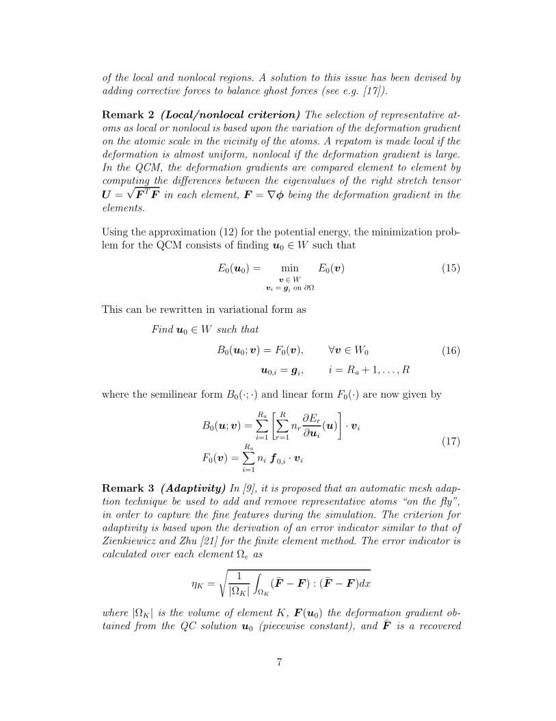
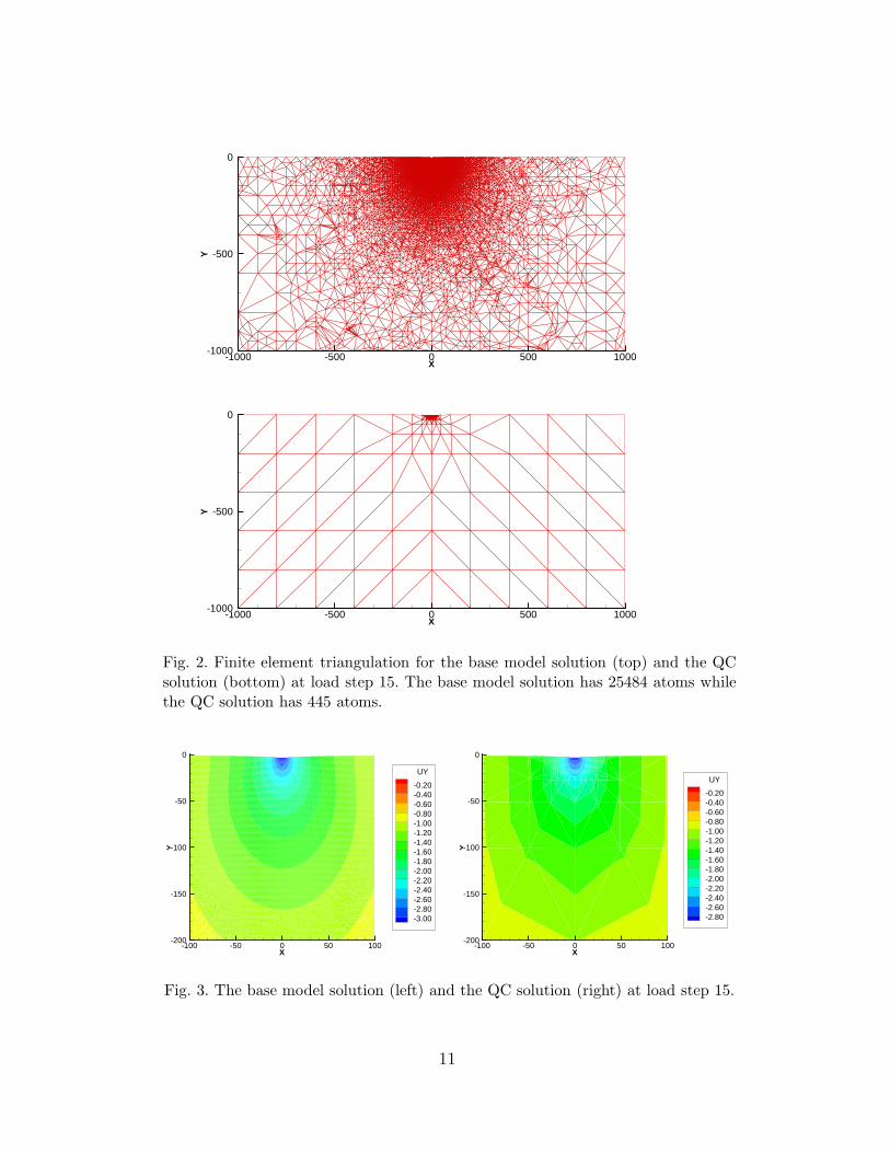
The meshes corresponding to these solutions are shown in Fig. 2. The verticaldisplacements, at an early stage of the indentation process, and just beforedislocation nucleation, are shown in Figs. 3 and 4, respectively. In the earlystages, it appears that the displacements computed by the QC solution com-pare well with the base model solution. However, at the dislocation nucleation,the latter appears to be softer, allowing the slip plane to move more quicklyinto the material.

For better comparison, we show in Fig. 5 the magnitude of the force exertedby the crystal onto the indenter. This force represents a quantity of physicalinterest as it clearly indicates the nucleation of the dislocation. Note that thebase model solution has been run only to load step 27 due to computationalcost. However, the QC solution has been displayed for the full 30 steps. TheQC solution seems to be stiffer, causing the dislocations to nucleate one loadstep sooner than the base model solution as the critical force is reached morequickly. Thus, although the displacements seem to compare well in the linearregion, small errors accumulate resulting in an inaccurate portrayal of themechanics of the lattice. Our goal in the next sections will be to establishestimates of the error in the quasicontinuum solution with respect to thisquantity of interest and to control that error via an adaptive algorithm.

3 Error estimation

3.1 Errors and quantity of interest. The errors in the QC solution u0, withrespect to the solution of the base problem, arise from three sources: (i) useof an iterative method to solve the nonlinear problem, (ii) reduction of thenumber of degrees of freedom from N to R, and (iii) approximation of thetotal potential energy by E0, as defined in (12) and (13).

The error due to the nonlinear solver is controlled at each iteration and isassumed to be negligible compared to the other sources of error. This erroris sometimes referred to as the solution error. The second type of error isanalogous to discretization error in Galerkin approximations such as in thefinite element method. Here it can be regarded as a model reduction error.Finally, the last source induces a so-called modeling error due to the modelingof the energy using the coupled local/nonlocal QCM. In this work, we willnot differentiate the three types of errors and will provide for estimates of thetotal error.

The next issue when dealing with a posteriori error estimation is the selectionof the error measure. Early works on the subject have concentrated on globalnorms such as energy norms. More recently, methods have been developed

10

X

Y

-1000 -500 0 500 1000-1000

-500

0

X

Y

-1000 -500 0 500 1000-1000

-500

0

Fig. 2. Finite element triangulation for the base model solution (top) and the QCsolution (bottom) at load step 15. The base model solution has 25484 atoms whilethe QC solution has 445 atoms.

X

Y

-100 -50 0 50 100-200

-150

-100

-50

0

UY

-0.20-0.40-0.60-0.80-1.00-1.20-1.40-1.60-1.80-2.00-2.20-2.40-2.60-2.80-3.00

X

Y

-100 -50 0 50 100-200

-150

-100

-50

0

UY

-0.20-0.40-0.60-0.80-1.00-1.20-1.40-1.60-1.80-2.00-2.20-2.40-2.60-2.80

Fig. 3. The base model solution (left) and the QC solution (right) at load step 15.

11

X

Y

-100 -50 0 50 100-200

-150

-100

-50

0

UY

-0.50-1.00-1.50-2.00-2.50-3.00-3.50-4.00-4.50-5.00

X

Y

-100 -50 0 50 100-200

-150

-100

-50

0

UY

-0.50-1.00-1.50-2.00-2.50-3.00-3.50-4.00-4.50-5.00

Fig. 4. The base model solution (left) and the QC solution (right) at the beginningof load step 27 and 26, respectively. The base model solution has 40554 atoms whilethe QC solution has 492 atoms.

0 1 2 3 4 5 6−1

0

1

2

3

4

5

Displacement

For

ce

Base ModelQC

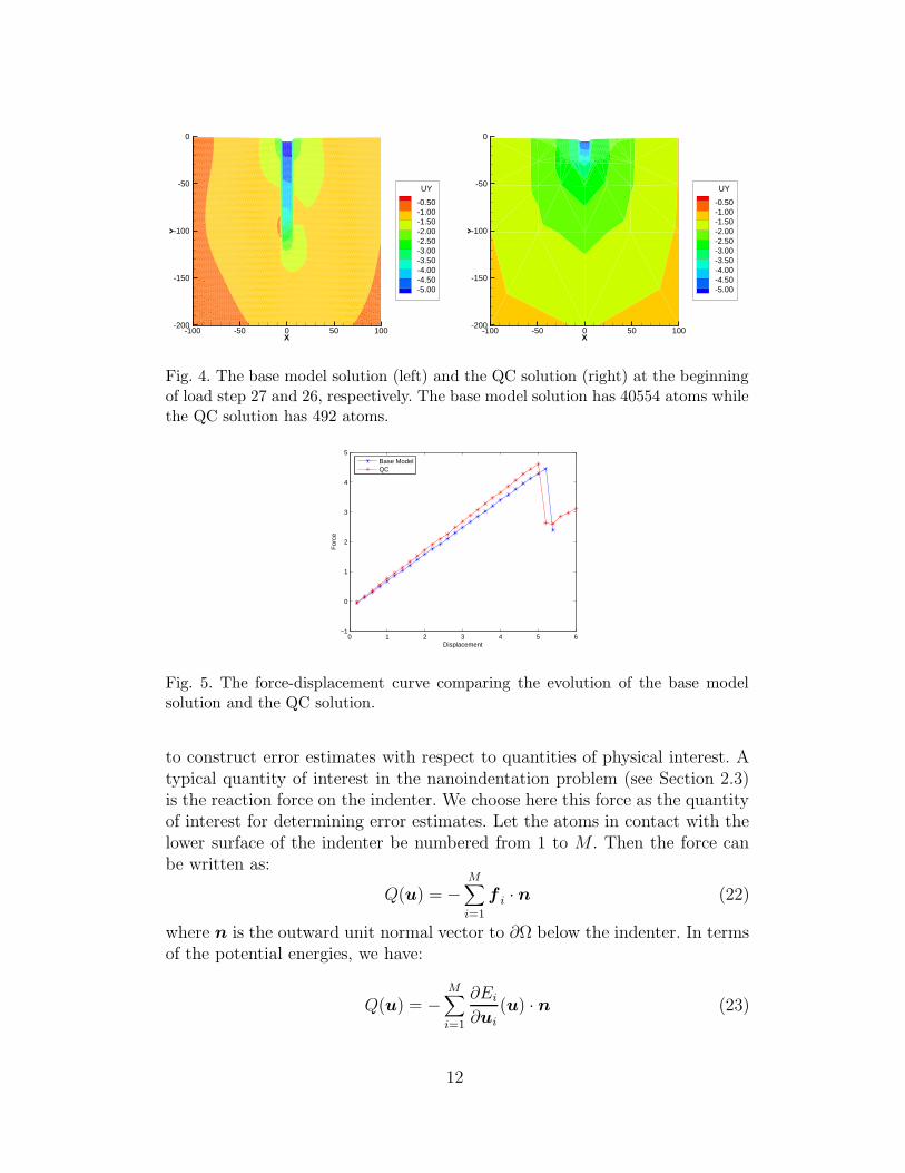
Fig. 5. The force-displacement curve comparing the evolution of the base modelsolution and the QC solution.

to construct error estimates with respect to quantities of physical interest. Atypical quantity of interest in the nanoindentation problem (see Section 2.3)is the reaction force on the indenter. We choose here this force as the quantityof interest for determining error estimates. Let the atoms in contact with thelower surface of the indenter be numbered from 1 to M . Then the force canbe written as:

Q(u) = −M∑

i=1

f i · n (22)

where n is the outward unit normal vector to ∂Ω below the indenter. In termsof the potential energies, we have:

Q(u) = −M∑

i=1

∂Ei

∂ui

(u) · n (23)

12

We note that Q(u) is a nonlinear functional defined on the solution space V .We also assume in the following that the meshes are constructed in such away that the M atoms under the indenter are representative atoms, and allthe forces are computed by the nonlocal approach.

The objective is then to estimate the error quantity

E = Q(u) − Q(πu0) (24)

where πu0 ∈ V is obtained from u0 by (10). To that end, we follow theapproach described in [11] and present the dual problem of the base model inthe next section.

3.2 The dual problem and error representation. The general approach toobtain estimates of the error E makes use of the solution of the dual problemassociated with the base model (7):

Find p ∈ V0 such that

B′(u; v, p) = Q′(u; v), ∀v ∈ V0(25)

where the derivatives are defined as

B′(u; v, p) = limθ→0

1

θ[B(u + θv; p) − B(u; p)]

Q′(u; v) = limθ→0

1

θ[Q(u + θv) − Q(u)]

(26)

In the molecular statics case, we have

B′(u; v, p) =Na∑

j=1

Na∑

i=1

vj ·[

N∑

k=1

∂2Ek

∂uj∂ui

(u)

]

· pi

Q′(u; v) = −Na∑

j=1

vj ·[

M∑

i=1

∂2Ei

∂uj∂ui

(u) · n]

(27)

However, since the dual solution depends on the exact solution u and thatthe above problem may be intractable due to the large number of atoms, wemay use instead approximations of p. An approximation can be obtained bysolving the surrogate dual problem:

Find p0 ∈ W0 such that

B′0(u0; v, p0) = Q′

0(u0; v), ∀v ∈ W0(28)

13

and by extending p0 to the space V0 to obtain the vector π0p0 ∈ V0,

π0p0,i =R∑

r=1

p0,rφr(xi), i = 1, . . . , N (29)

The quantity of interest Q0 in (28) is defined for v ∈ W by Q0(v) = Q(πv).

In the following, we denote by e0 and ε0 the errors in πu0 and π0p0, i.e.

e0 = u − πu0 ∈ V

ε0 = p − π0p0 ∈ V0(30)

We apply the results of [11] to derive the following theorem that provides fora representation of the error in the quantity of interest:

Theorem 1 Let the semilinear form B(·; ·) in (7) belong to C3(V ) and let thequantity of interest Q(·) as defined in (23) be in C3(V ). Let u ∈ V and p ∈ V0

be solutions of the base problems (7) and (25), respectively. Let (u0, p0) ∈W × W0 be the solution pair of the surrogate problems and let (πu0, π0p0)denote their extensions to the spaces V ×V0. Then the error in Q(u) producedby πu0 is given by

E = Q(u) − Q(πu0) = R(πu0; p) + ∆(πu0, π0p0, e0, ε0) (31)

where R(πu0; v) is the residual functional,

R(πu0; v) = F (v) − B(πu0; v), v ∈ V0 (32)

and ∆ = ∆(πu0, π0p0, e0, ε0) is the remainder,

∆ =1

2

∫ 1

0B′′(πu0 + se0; e0, e0, π0p0 + sε0)

− Q′′(πu0 + se0; e0, e0)ds

+1

2

∫ 1

0Q′′′(πu0 + se0; e0, e0) − 3B′′(πu0 + se0; e0, e0, ε0)

− B′′′(πu0 + se0; e0, e0, e0, π0p0 + sε0)(s − 1)sds

(33)

Goal-oriented error estimators aim at estimating E by accurately approximat-ing the quantity R(πu0; p) and neglecting the higher-order terms ∆. One suchapproach is proposed in the next section.

3.3 The error estimator. We first rewrite the quantity R(πu0; p) in differentforms in order to lay down our motivations for the derivation of the error

14

estimator. Starting from the definition of the residual, it is clear that:

R(πu0; p) = F (πu0, p) − B(πu0; p)

=Na∑

i=1

f i · pi −Na∑

i=1

[

N∑

k=1

∂Ek

∂ui

(πu0)

]

· pi

=Na∑

i=1

(

f i −[

N∑

k=1

∂Ek

∂ui

(πu0)

])

· pi

=Na∑

i=1

ri(πu0) · pi

(34)

where the residual vector r(πu0) ∈ V0 indicates how the forces acting on eachatom i fail to be equilibrated. We observe that the calculation of R(πu0; p)may be cost prohibitive when the number of atoms N , or rather Na, is large. Inan effort to reduce the computational cost of the error estimator, it is desirableto take into account only those contributions that are the most significant,meaning that the number of atoms to be considered for the calculation of (34)should range from Ra to Na.

Moreover, thanks to the linearity of the residual functional, the quantityR(πu0; p) can be decomposed as:

R(πu0; p) = R(πu0; π0p0) + R(πu0; ε0) (35)

It is well known that the contribution R(πu0; π0p0) vanishes for Galerkinapproximations. In a similar manner here, this term fails to detect the modelreduction error. It follows that the solution p0 provides for a poor approxi-mation of the dual solution p, in the sense that R(πu0; π0p0) approximatesR(πu0; p) poorly, and a better approximation should be obtained in a spacelarger than W0.

We propose here to evaluate the residual and the dual solution on a meshwhich is finer than the mesh used for the evaluation of u0, but much coarserthan the mesh that would be obtained by considering all atoms as representiveatoms. Let Ph denote such a partition of Ω (we shall explain below how toconstruct Ph) and suppose that it contains a total number of N nodes with Na

interior nodes. We introduce the vector spaces V = (Rd)N and V0 = (Rd)Na

as well as the extension operators π : V → V and π0 : V0 → V0. We can nowdefine a residual functional R on V such that for any u ∈ V and v ∈ V0

R(u; v) =Na∑

i=1

ri(u) · vi (36)

where the ri(u) are computed via the coupled local/nonlocal quasicontinuum

15

approach. We will also consider the approximate dual problem:

Find p ∈ V0 such that

B′(πu0; v, p) = Q′(πu0; v), ∀v ∈ V0

(37)

with, for all u ∈ V and v ∈ V0,

B(u; v) =Na∑

i=1

N∑

k=1

nk

∂Ek

∂ui

(u)

· vi

Q(u) = −M∑

i=1

∂Ei

∂u,i

(u) · n(38)

Note that B is computed using the N representative atoms in the partitionPh. We emphasize here that the approximation p of p involves the same typesof errors as in u0, but that it also strongly depends on the accuracy of thecomputed solution u0.

We now define the error estimator with respect to the quantity of interest, Q,as the computable quantity

η = R(πu0; p) =Na∑

i=1

ri(πu0) · pi (39)

and we show in the next section that η is a reasonable estimate of the errorE = Q(u) − Q0(u0) = Q(u) − Q(πu0). Finally, the finite element partitionPh, or enriched mesh, for the calculation of the dual approximation p and theresidual r is constructed using the adaptive technique described in Remark 3using a smaller tolerance than 0.075. In order to assess the quality of the errorestimate, we will use the effectivity index defined as the ratio ζ = η/E .

3.4 Numerical experiments. We perform here a few numerical experimentsusing the same setting as in Section 2.3 in order to study the performance of theerror estimator. We first investigate the influence of approximating the dualsolution in the enriched space V rather than in the space V0. Close-up viewsof the meshes (QCM and enriched meshes) corresponding to these spaces areshown in Fig. 6. As expected, the error estimator performs very poorly whenthe dual solution is approximated on the QCM mesh. This is clearly indicatedin Fig. 7 where it is shown that the error estimator detects very little error atall load steps. By contrast, the error estimator provides reasonable estimateswhen the enriched space V is used for the approximation of the dual solution,as shown in Fig. 8. The effectivity indices remain mostly close to unity, exceptmaybe in the region of dislocation nucleation where strong nonlinear behavior

16

X

Y

-100 -50 0 50 100-200

-150

-100

-50

0

X

Y

-100 -50 0 50 100-200

-150

-100

-50

0

Fig. 6. QCM mesh (left) and enriched mesh (right) at load step 9. The QCM meshhas 432 atoms while the enriched mesh contains 10887.

0 1 2 3 4 5 60

0.1

0.2

0.3

0.4

0.5

0.6

0.7

Displacement

Rel

ativ

e E

rror

Exact ErrorError Est

Fig. 7. The (relative) exact error and the error estimate on the QCM mesh withoutenrichment.

occurs. Indeed, recall that the QC solution dislocates one load step early.In other words, the primal solution u0 contains large errors that certainlypollute the approximation of the dual solution at that particular load step.We actually show in Fig. 9 the dual solutions p and p0 computed using thebase model and QCM, respectively, and p exhibits many more details thanp0, notably in the region away from the indenter near the slip plane.

4 Adaptivity

We propose here a simple adaptive strategy to control the error in the quantityof interest within some prescribed tolerance δtol. Our approach is different fromthe one used in the QCM code, but was made to fit the data structure available

17

0 1 2 3 4 5 60.05

0.1

0.15

0.2

0.25

0.3

0.35

0.4

0.45

0.5

0.55

Displacement

Rel

ativ

e E

rror

Exact ErrorError Est

0 1 2 3 4 5 6−0.4

−0.2

0

0.2

0.4

0.6

0.8

1

1.2

1.4

1.6

Displacement

Effe

ctiv

ity In

dex

Fig. 8. The relative error (left) and the effectivity indices (right) are shown com-paring the error estimator to the exact error for the enriched QCM mesh.

X

Y

-100 -50 0 50 100-200

-150

-100

-50

0

PY

0.900.800.700.600.500.400.300.200.10

X

Y

-100 -50 0 50 100-200

-150

-100

-50

0

PY

0.900.800.700.600.500.400.300.200.10

Fig. 9. The dual solution of the base model (left) and the QCM (right) at thebeginning of load step 27.

in the code.

4.1 Adaptive strategy. For the purpose of spatial adaptation with respect tothe quantity of interest, it is first necessary to decompose the error estimateη into local contributions that could be employed for the development of re-finement indicators. Due to the structure of the code, we have adopted anapproach in which the local contributions are defined per element such that:

η =Ne∑

K=1

ηK (40)

This is accomplished in practice as follows: for each element K of the partition,one computes the nodal contributions ηK

i = ri(πu0)·pi of the quantity η, from

18

which one can calculate an elementwise contribution as:

ηK(πu0, p) =3

|K|NKi

∫

ΩK

Nd∑

i=1

ηKi φi dx, (41)

where |K| denotes the area of element K, Nd the number of nodes in K, NKi

the number of elements sharing node i, and φi the restrictions to element K ofthe linear base functions as defined in (9). This decomposition is simple andeasily implemented in the QCM code, but is not unique.

The adaptive algorithm, the so-called Goals algorithm [13], proceeds as follows:

(1) Initialize the load step to s = 0. Input user-tolerance δtol.(2) Go to the next load step, s = s + 1.(3) Solve the primal and dual problems as described in Sections 2.2 and 3.2,

respectively.(4) Compute the error estimate as discussed in Section 3.3.(5) If |η| < δtol|Q(u0)|, go to step (2). Otherwise, mark those elements that

satisfy |ηK(πu0, p)| > γ maxK

|ηK(πu0, p)|, where γ is a user-supplied

number between 0 and 1.(6) Refine flagged elements and go to step (3).

Note that our adaptive algorithm slightly differs from QCM in the sense that,in the QCM, the elements are flagged for refinement if the elemental contribu-tions are below some user-specified number γQC and that the adaptive processwithin each load step eventually ends when no more elements are flagged forrefinement.

4.2 Numerical examples. In the following examples, we choose δtol = 0.05(the solution is controlled so that the relative error is always less than fivepercent) and γ = 0.25. In Fig. 10, we show the adapted meshes obtainedusing the QCM and the Goals algorithm once dislocations have nucleated. Ascan be seen, the Goals mesh includes many more atoms near the indenter.Fig. 11 shows the evolution of the number of atoms (degrees of freedom) forboth methods. It is interesting to see that the Goals algorithm adds manyrepatoms at the beginning of the simulation while QCM essentially refines atthe dislocation nucleation.

Force-displacement curves are shown in Fig. 12. We observe that the Goalsalgorithm is able to control the error within the specified tolerance and pro-vides a solution that predicts the dislocation nucleation just as the base modelsolution does, but at a much lower computational cost. Relative errors andeffectivity indices are plotted in Fig. 13, demonstrating the effectiveness of

19

X

Y

-100 -50 0 50 100-200

-150

-100

-50

0

X

Y

-100 -50 0 50 100-200

-150

-100

-50

0

Fig. 10. QCM (left) and Goals (right) mesh at load step 27. The number of atomsin the QCM and Goals meshes are 1629 and 3452, respectively.

0 5 10 15 20 25 300

500

1000

1500

2000

2500

3000

3500

4000

Load Step

Num

ber

of A

tom

s

QCGoals

Fig. 11. Comparison of the evolution of QCM mesh and Goals mesh.

our error estimator. Finally, we show in Fig. 14 the dual solutions obtainedusing the base model, the QCM, and the Goals algorithm. Again, this resultshows that the dual solutions for the base model and the Goals algorithm arevirtually indistinguishable while the solution of the QCM is very different.

5 Conclusions

In the present work, we have extended the methodology of goal-oriented errorestimation and adaptivity to molecular statics using approximate solutionsproduced by the quasicontinuum method (QCM). Estimates of the error inthe QC approximations with respect to quantities of interest are derived andare used as a basis for the development of a Goals algorithm. The theoreticalresults were applied to a sample nanoindentation problem and it was foundthat the Goals methodology provides reliable error estimates and successfully

20

0 1 2 3 4 5 6−1

0

1

2

3

4

5

DisplacementF

orce

Base ModelGoalsQC

Fig. 12. Force-displacement curves computed from the base model solution, the QCsolution, and the Goals solution.

0 1 2 3 4 5 60

0.05

0.1

0.15

0.2

0.25

Displacement

Rel

ativ

e E

rror

Error EstExact Error

0 1 2 3 4 5 6−1

0

1

2

3

4

5

Displacement

Effe

ctiv

ity In

dex

Fig. 13. Relative error (left) and effectivity indices (right).

controls the prediction of the force acting on the indenter. The results wereconsistently verified using a highly resolved solution of the nanoindentationproblem.

Acknowledgments. Paul T. Bauman gratefully acknowledges the Depart-ment of Energy Computational Science Graduate Fellowship for financial sup-port. Support of this work by ONR under Contract No. N00014-99-1-0124 isgratefully acknowledged.

21

X

Y

-100 -50 0 50 100-200

-150

-100

-50

0

PY

0.900.800.700.600.500.400.300.200.10

X

Y

-100 -50 0 50 100-200

-150

-100

-50

0

PY

0.900.800.700.600.500.400.300.200.10

X

Y

-100 -50 0 50 100-200

-150

-100

-50

0

PY

0.900.800.700.600.500.400.300.200.10

Fig. 14. Comparison of the dual solution for the base model (top left), the Goalsalgorithm (top right), and the QCM (bottom) at the end of load step 27.

References

[1] J. Q. Broughton, F. F. Abraham, N. Bernstein, and E. Kaxiras. Concurrentcoupling of length scales: Methodology and application. Physical Review B,60(4):2391–2403, 1999.

[2] W. A. Curtin and R. E. Miller. Atomistic/continuum coupling in computationalmaterials science. Modelling Simul. Mater. Sci. Eng., 11:R33–R68, 2003.

[3] M. S. Daw and M. I. Baskes. Semiempirical, quantum mechanical calculation ofhydrogen embrittlement in metals. Physical Review Letters, 50(17):1285–1288,1983.

[4] M. S. Daw and M. I. Baskes. Embedded-atom method: Derivation andapplications to impurities, surfaces, and other defects in metals. Physical Review

B, 29(12):6443–6453, 1984.

[5] F. Ercolessi and J. Adams. Interatomic potentials from 1st-principles

22

calculations – the force-matching method. Europhysics Letters, 26:583–588,1993.

[6] S. M. Foiles, M. I. Baskes, and M. S. Daw. Embedded-atom-method functionsfor fcc metals Cu, Ag, Au, Ni, Pd, Pt, and their alloys. Physical Review B,33(12):7983–7991, 1986.

[7] G. Friesecke and F. Theil. Validity and failure of the Cauchy-Born hypothesisin a two-dimensional mass-spring lattice. J. Nonlinear Sci., 12:445–478, 2002.

[8] W. K. Liu, E. G. Karpov, S. Zhang, and H. S. Park. An introduction tocomputational nanomechanics and materials. Comput. Methods Appl. Mech.

Engng., 193:1529–1578, 2004.

[9] R. E. Miller and E. B. Tadmor. The quasicontinuum method: Overview,applications, and current directions. Journal of Computer-Aided Design, 9:203–239, 2002.

[10] R. E. Miller and E. B. Tadmor. QC Tutorial Guide Version 1.1, May 2004.Available at www.qcmethod.com.

[11] J. T. Oden and S. Prudhomme. Estimation of modeling error in computationalmechanics. Journal of Computational Physics, 182:496–515, 2002.

[12] J. T. Oden, S. Prudhomme, and P. Bauman. On the extension of goal-orientederror estimation and hierarchical modeling to discrete lattice models. Comput.

Methods Appl. Mech. Engrg., 194:3668–3688, 2005.

[13] J. T. Oden, S. Prudhomme, A. Romkes, and P. Bauman. Multi-scale modelingof physical phenomena: Adaptive control of models. ICES Report 05-20, TheUniversity of Texas at Austin, 2005. Submitted to SIAM Journal on ScientificComputing.

[14] J. T. Oden and K. Vemaganti. Estimation of local modeling error and goal-oriented modeling of heterogeneous materials 1. Error estimates and adaptivealgorithms. Journal of Computational Physics, 164:22–47, 2000.

[15] R. Phillips, D. Rodney, V. Shenoy, E. B. Tadmor, and M. Ortiz. Hierarchicalmodels of plasticity: dislocation nucleation and interaction. Modeling Simul.

Mater. Sci. Eng., 7:769–780, 1999.

[16] A. Romkes and J. T. Oden. Adaptive modeling of wave propagation inheterogeneous elastic solids. Comput. Methods Appl. Mech. Engng., 193:539–559, 2004.

[17] V. B. Shenoy, R. Miller, E. B. Tadmor, D. Rodney, R. Phillips, andM. Ortiz. An adaptive finite element approach to atomic-scale mechanics —the quasicontinuum method. Journal of the Mechanics and Physics of Solids,47:611–642, 1999.

23

[18] E. B. Tadmor. The Quasicontinuum Method. PhD thesis, Brown University,1996.

[19] E. B. Tadmor, R. Miller, R. Phillips, and M. Ortiz. Nanoindentation andincipient plasticity. J. Mater. Res., 14:2233–2250, 1999.

[20] E. B. Tadmor, M. Ortiz, and R. Phillips. Quasicontinuum analysis of defectsin solids. Phil. Mag. A, 73(6):1529–1563, 1996.

[21] O. C. Zienkiewicz and J. Z. Zhu. A simple error estimator and adaptiveprocedure for practical engineering analysis. Int. J. Numer. Methods Engrg.,24:337–357, 1987.

24