Error and Uncertainty in EISCAT data

• When we’re designing an experiment, we have to bear in mind six requirements:

1. Spatial Resolution2. Range Extent3. Lag Extent4. Lag Resolution5. Time Resolution6. Accuracy

• Unfortunately, these requirements are frequently contradictory!

• Real experiment design is a compromise that gives acceptable (rather thanoptimum) solutions to these requirements.

Requirements of an experiment

1) Spatial Resolution

• To measure the ionosphere properly, we need to measure it on at least the same height scale as its own natural altitude variation. If we do not do this, we will average height-varying parameters together and arrive at a result which fails to represent any one altitude properly.

• One measure of the rate of parameter change with height in the ionosphere is given by the plasma scale height. Remember that the scale height is defined as an e-folding distance, so ideally we want to have gates at significantly better resolution than the scale height.

gm

TTkH

i

iep

)(

• If we want gates separated by one quarter of the ionospheric scale height;

• At E region altitudes; mi ~ 30 amu and Ti ~ Te ~ 200 K so Hp ~ 12 km and so we should have gates separated by about 3 km.

• At F region altitudes, mi ~ 16 amu and Ti ~ 1000 K Te ~ 2000 K so Hp ~ 150 km and so it is acceptable for the gate separation to be ~ 40 km.

• Ideally, we would want each gate to be independent (range ambiguity = gate separation) although we could relax this where the scale height was large.

Possible values for UHF experiment

Constraining factors for an incoherent scatter radar experiment

Some constraining factors for incoherent scatter experiments, shown as functions of height for typical ionospheric conditions.

Time of flight forradar pulse

Pulse length givingresolution equal tothe scale-height.

ionosphericcorrelation time,τ1 for UHF

ionosphericcorrelation time,τ1 for VHF

Minimum pulse length obtainable from transmitter

2) Range Extent

• This is really about making sure that our measurements address the kind of physics we are trying to understand.

• In some experiments with specific scientific aims (e.g. PMSE studies, topside ionoutflows, wave coupling across the mesopause) it may be acceptable to probe only a limited range of altitudes.

• However, for general purpose experiments (e.g. the most frequently used Common Programmes) we would like to survey the whole ionosphere from the lowest to the highest altitudes where we can get useful signals.

• This imposes the requirement that our experiment should include different types ofmodulation such that:

1) E region data can be obtained with adequate range resolution and range ambiguity

2) F region data can be obtained with adequate signal-to-noise.

• Very long pulses can be used in the topside, where range resolution is not a pressingRequirement, in order to boost SNR to acceptable levels.

• To use our radar optimally, we would like to transmit as much power as the duty cycle of the transmitter allows.

• To fulfill the requirement for different range resolutions and ambiguities, we ought to transmit several different modulations (e.g. alternating code, long pulse, power profile etc). We transmit each modulation on a different frequency.

• Even though we can only transmit one frequency at a time, we can receive and process signals on many frequencies simultaneously, since we have a multi-channel system.

• This means that the low-altitude modulations have to be transmitted last !

• As we have seen, there is one modulation scheme which is almost optimal for all altitudes (the alternating code).

3) Lag Extent

• In order to get full information on the shape of our ACF, we have to sample the full length of the function from the zero lag to where the correlation disappears to zero (equivalent to the decay time of the plasma waves we’re scattering from).

• The longest ACFs (narrowest spectra) are found in the E-region and the shortest ACFs (broad spectra) come from the F-region.

• Hence we need the largest lag extent at the lowest altitude.

• This is exactly the opposite of what we’d like, given that for conventional long pulses, a long delay time implies a large spatial ambiguity.

• We can’t use long pulses at altitudes where their spatial ambiguity exceeds the scale height. However, short pulses won’t give us a large enough lag extent.

• We need to find some “trick” by which we can get a large lag extent with a small range ambiguity, and this is why we need pulse coding.

4) Lag Resolution

• It isn’t merely sufficient to sample the ACF out to a long enough lag. We also have to sample it sufficiently frequently to define its shape.

• Since our lags come from cross-products of samples, our shortest possible lag spacing is going to be equal to our sample spacing.

• However, the sample spacing is set by the post-detection filter we use, and this in turn is determined by the modulation bandwidth as well as the spectral width.

• If we OVERSAMPLE the filter, i.e. sample faster than twice the fastest frequency which the filter allows through, we don’t gain any new information.

• If we UNDERSAMPLE the filter, i.e. sample slowly so that we don’t sample the full range of frequencies allowed through by the filter, then we’re losing information. This is equivalent to determining the ACF with insufficient resolution.

Aliasing due to undersampling of data

• Oversampling isn’t dangerous, but it is a waste of effort.

• Undersampling can be a serious problem and lead to (very) wrong results.

• The choice of filter we need has to be made with the required lag resolution in mind

5) Time Resolution and 6) Accuracy

• These two are coupled ….

• Ideally we’d like to measure our data at very high time resolution, so we could get information on very short timescale processes e.g. in aurora. 

• Unfortunately the fact that we’re measuring a stochastic process means that we have to post-integrate a large number of measurements together before the expectation value of the ACF becomes visible above the random noise.

• For a given Signal-to-Noise Ratio, the accuracy of a measured signal power improves as the square root of the observing time, according to the following formula:

tbn

P

P

P

P s

n

s

s

1

Ps is the measured signal powerPn is the noise powerb is the measurement bandwidthn is the number of pulses transmitted in unit time is the pulse lengtht is the integration time.

• This accuracy calculation can ultimately be applied to the fitted plasma parameters.

i

i

e

e

e

e

s

s

T

T

T

T

N

N

P

P

2~

2~~

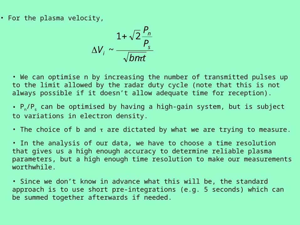
• For the plasma velocity,

tbn

P

P

V s

n

i

21

~

• We can optimise n by increasing the number of transmitted pulses up to the limit allowed by the radar duty cycle (note that this is not always possible if it doesn’t allow adequate time for reception). • Pn/Ps can be optimised by having a high-gain system, but is subject to variations in electron density. • The choice of b and are dictated by what we are trying to measure. • In the analysis of our data, we have to choose a time resolution that gives us a high enough accuracy to determine reliable plasma parameters, but a high enough time resolution to make our measurements worthwhile. • Since we don’t know in advance what this will be, the standard approach is to use short pre-integrations (e.g. 5 seconds) which can be summed together afterwards if needed.

Parts of an experiment

The aim of our experiment is to measure lag profiles from the ionospheric scattered signal, so that we can fit profiles of plasma parameters. However, in order to do this, we have to measure other things as well…

Noise Background

All of our measurements, as well as containing the wanted signal, contain a large percentage of “background noise”. This is cosmic noise from the sky, electronic noise from the radar system, external interference etc. We want to subtract this background from our wanted signal, and we first assume that the background noise is stationary with respect to time at least on the timescales of our measurement (seconds). In this case, if we make an independent measurement of the background only (i.e. without the signal) in the same way as our signal+background measurement, we can subtract the two, leaving only the wanted signal.

We can measure the noise only by either:

a) Measuring the background before we transmit the signal, thus ensuring no possibility of contamination.

b) Waiting until the signal pulse has propagated out of the ionosphere before measuring the background.

If we further assume that the background is “white” i.e. that it is evenly spread in frequency across our passband, then we don’t need to measure the spectral shape of the background, only its power, so only the background zero lag has to be measured.

Noise Injection

Sometimes “noise” can actually be helpful to us. We can use a standard noise injection signal (i.e. an injected signal at known power) to calibrate the system.

To do this, the noise injection has to be broadband across all the used frequencies, and has to be measured in the same way as the signal+background and background.

Since any measurement of the injected noise will also contain the background, we have to subtract the background from our noise injection measurement before calibrating the radar by comparing the noise injection to the level of the wanted signal. Since the injected signal is broadband, only the zero lag has to be computed.  Thus many data dumps contain three distinct parts – signal, background and calibration (noise injection).

“Clutter”

Because the ionospheric signal is so weak, it is easy for it to be swamped by even low-amplitude signals from other sources. The most troublesome can be signals caused by the radar transmission reflecting from mountains etc, or from satellites and orbital debris. These kinds of signals are known as “clutter”. In Tromsø, because the radar is in a valley, any reflections from mountains that we get come from very close range, and are eliminated by gating the receiver correctly. At Svalbard, because the radar is on a mountain, we can get reflections (e.g. via the radar side lobes) from mountains many tens of kilometres away (i.e. at ranges comparable to the ionosphere). To eliminate these we use our knowledge that, while the correlation time of plasma waves is short (hundreds of microseconds) the correlation time of mountains is somewhat longer (millions of years). 

Instead of sending one set of sounding modulations, we transmit two, spaced apart by more than the correlation time of the plasma waves and less than the correlation time of mountains. Before we start to form lags etc from the two sample streams, we first subtract one from the other. This eliminates the clutter, which is present to the same degree in both, but since the wave process is stochastic, we can form the same expectation value by correlating and integrating the result of the subtraction as we could from either of the individual data streams. The difference is that the result of the subtraction contains no clutter. This is a standard process in non-ionospheric radars (which are interested in resolving moving targets, from non-moving targets.

The Solution….

Satellites

At the other end of our range coverage, we can get large coherent echoes if our transmitted pulse strikes a satellite (remember that the illuminated volume can be thousands of km3). However, it may be that satellites are only instantaneously in the beam. Certainly they are moving rapidly through the sidelobe pattern, so we can’t use the moving target method here. For topside data (where satellite contamination is a real problem) we have to do some post-processing of the data to find and eliminate satellite events. Failure to eliminate even a short-lived event can have a serious effect on long data integrations.

“Self-Clutter”

Note that if the experiment is not well designed, some of our transmissions can occur as “clutter” in the reception of others. Consider the simple case of a two-pulse experiment, where the pulses are transmitted very close together.

Note that for the zero lag, the signal is ambiguous, because the range ambiguity of both pulses appears at ionospheric ranges. In some applications (e.g. multipulse codes) this is an unwanted by-product, but a price worth paying to get small (unique) spatial ambiguities at the other lags. The fact that we generally transmit several modulations consecutively before receiving explains why we need a multi-frequency radar !

Two dimensional ambiguity functionsof a two-pulse code

Sources of random and systematic errors in EISCAT data.

The accuracy of any parameter derived in this way depends on the quality of the data (SNR) and the accuracy of the fitting procedures during the data analysis.

The uncertainties in these parameters are then estimated from the variance of measurements at different lags in the ACF.

In EISCAT data analysis, parameters are obtained by fitting a theoretical ACF to the observed ACF.

Extensive studies have been made into the nature of uncertainties in EISCAT data. Most of this work has been carried out by the EISCAT group at Aberystwyth.

Using data from an early experiment (CP-4-A, in which measurements were made on 6 separate frequencies which were then stored separately) they were able to compare random uncertainties (as estimated from the standard deviation of the parameters averaged over the 6 channels) with theoretical formulae and the uncertainty estimated from the fit variances.

All three were found to be in good agreement.

2

3

5.0

25.0

1

11

10.7116.01

2117.1

RmTT

T

rt

T

RV

ii

eip

Bnt

Rmm

RTT ee 2

112130.2

Bnt

Rmm

RTT ii 2

112130.2

Bnt

RNN ee

1Where R is the SNR over the ion-line bandwidth, B, m is number of independent background gates, t is the integration time, τ is the pulse length and n is the number of frequencies used.

Formulae for estimating uncertainty in EISCAT data;

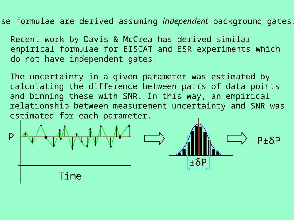
These formulae are derived assuming independent background gates.

Recent work by Davis & McCrea has derived similar empirical formulae for EISCAT and ESR experiments which do not have independent gates.

The uncertainty in a given parameter was estimated by calculating the difference between pairs of data points and binning these with SNR. In this way, an empirical relationship between measurement uncertainty and SNR was estimated for each parameter.

P±δP

±δP

P

Time

Using this method, good agreement was found with the theoretical formulae for Vp and Te but uncertainties in Ti and Ne were much greater than predicted by theory.

The results of this investigation are applicable only to the experimental data used but the method is applicable to all EISCAT (and indeed, ISR) data.

The advantage of this method is that you do not need to know anything about the radar pulse scheme and so it is easily applicable to complex experiments for which theoretical uncertainties would be hard to formulate.

Sources of Systematic error in EISCAT data

Models – Standard EISCAT analysis uses multi-parameter fitting between measured and theoretical functions (ACFs or spectra)

However, these depend on (at least) five plasma parameters:Electron density, electron temperature, ion temperature, ion composition, ion-neutral collision frequency (Ion velocity also produces a Doppler shift – but does not change spectral shape)

If we attempt to fit all these parameters at once to a (noisy) measurement, the fit will fail in most cases

Therefore we need to constrain the fit by assuming a certain amount of a priori knowledge

Typically we assume that the ion-neutral collision frequency and sometimes the ion composition are known, and described by models.

What if the models are wrong ?

• The ion-neutral collision frequency is significant only in the E-region, where it affects the width of the (single-peaked) spectrum

• An error in the collision frequency mainly affects the temperature estimate (if coll. freq is assumed too low, resulting temperature is too high).

• Ion composition is important in the E-F transition region, and in the topside

• An error in the ion composition mainly affects the ion and electron temperatures

• Ion mass assumed too high gives too high values for ion and electron temperatures.

Non-thermal plasmas

Standard EISCAT analysis assumes that the plasma is thermal.

Large electric fields over auroral regions cause the plasma to movewith large velocities ( > 2000 m/s).

The neutral air is not directly affected by the electric field, and so the plasma and neutral air move at different velocities.

Since the neutral air is 10,000 times denser than the plasma (in the F-region), the two species collide. This leads to;

a) Ion-frictional heating

b) Non-Maxwellian distributions.

Ion frictional heating

Momentum is transferred through ion-neutral collisions, leading to An increase in ion temperature.

2)(3 nin

ni uuk

mTT

Where Ti, Tn are the ion and neutral temperatures, mn is the mass of a neutral particle, k is Boltzmann’s constant and ui,un are the ion and neutral velocities.

A change in ion velocity of 2000 m/s would lead to an increasein ion temperature of 2600 K.

The chemical reaction rates of the O+ ions are temperature dependent.An increase in temperature increases the rate of reactions which convert O+ ions into molecular species such as NO+ and O2

+.

As the proportion of molecular ions increases, so does the meanion mass. If O+ has been assumed in the model used to analyseEISCAT data, the ion mass is under-estimated (up to a factor of 2)during times of ion heating.

Going back to how the various parameters are derived from the incoherent scatter spectrum;

If Ti is underestimated, so is TeIf mi is underestimated, Ti is underestimated.

Ti/mi is estimated from width of the spectrum.

Te/Ti is estimated from the sharpness of the peaks in the spectrum.

So, what does this look like in the data?

Temperature (K)

Velocity(m/s)

Δui ~ 1200 ms-1

ΔTi ~ 900 K

ΔTi ~ 550 K

2)(3 in

i uk

mT

It is likely that mi has been under-estimated in the EISCAT analysis.

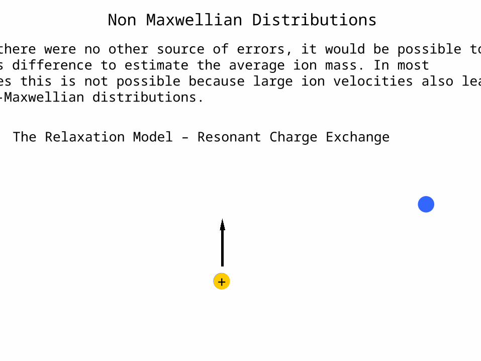
If there were no other source of errors, it would be possible to usethis difference to estimate the average ion mass. In mostcases this is not possible because large ion velocities also lead tonon-Maxwellian distributions.

The Relaxation Model – Resonant Charge Exchange

+

+

Non Maxwellian Distributions

V┴1

V┴2

ETn

BTi

RCE creates ions with neutral velocityThese gyrate around the B-fieldIn the F-region, under a strong E-field, the ions form a toroidal thermal velocity distribution

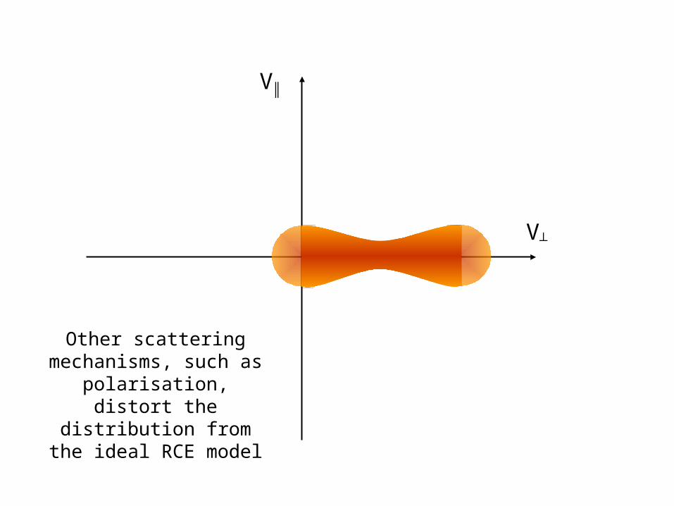
V║

V┴

Other scattering mechanisms, such as polarisation, distort the distribution from the ideal RCE model

Since this distribution is anisotropic, the temperature measured will depend on the angle at which the measurements are made.

For a distribution that is axi-symmetric, the mean temperature is

Ti = T║+2T┴

3

Tφ = -T║cos2φ+2T┴sin2φ

For such a distribution, the temperature at an angle, φ, can be expressed as;

Combining these two, the mean temperature can be measured by observing the distribution at an aspect angle of 54.7o

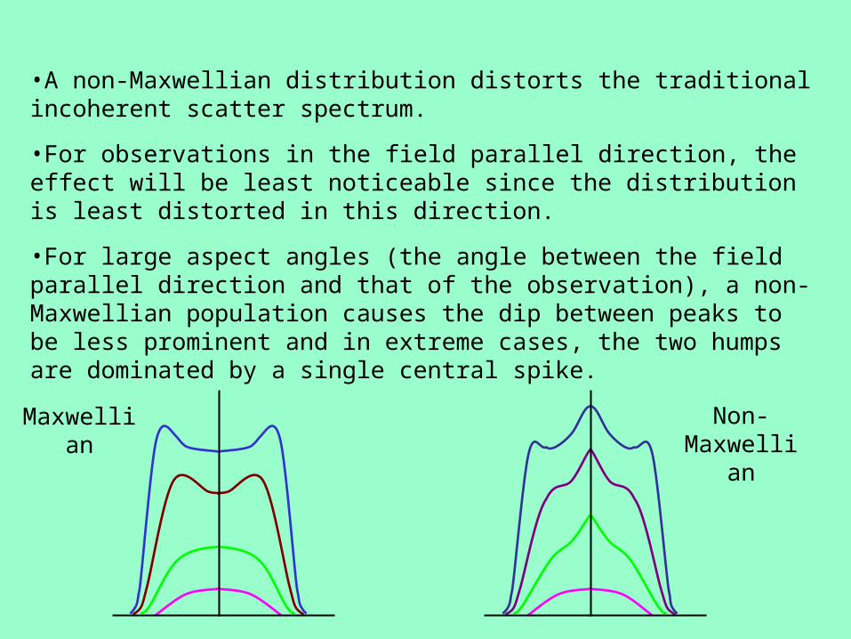
•A non-Maxwellian distribution distorts the traditional incoherent scatter spectrum.

•For observations in the field parallel direction, the effect will be least noticeable since the distribution is least distorted in this direction.

•For large aspect angles (the angle between the field parallel direction and that of the observation), a non-Maxwellian population causes the dip between peaks to be less prominent and in extreme cases, the two humps are dominated by a single central spike.

Maxwellian Non-Maxwellian