ERDC/CRREL TR-16-1 'The Benefits and Limitations of Hydraulic Modeling ... · The Benefits and...

ERD

C/CR

REL

TR-1

6-1

Wetland Regulatory Assistance Program (WRAP)

The Benefits and Limitations of Hydraulic Modeling for Ordinary High Water Mark Delineation

Cold

Reg

ions

Res

earc

h

and

Engi

neer

ing

Labo

rato

ry

John D. Gartner, Matthew K. Mersel, Lindsey E. Lefebvre, and Robert W. Lichvar

February 2016

Approved for public release; distribution is unlimited.

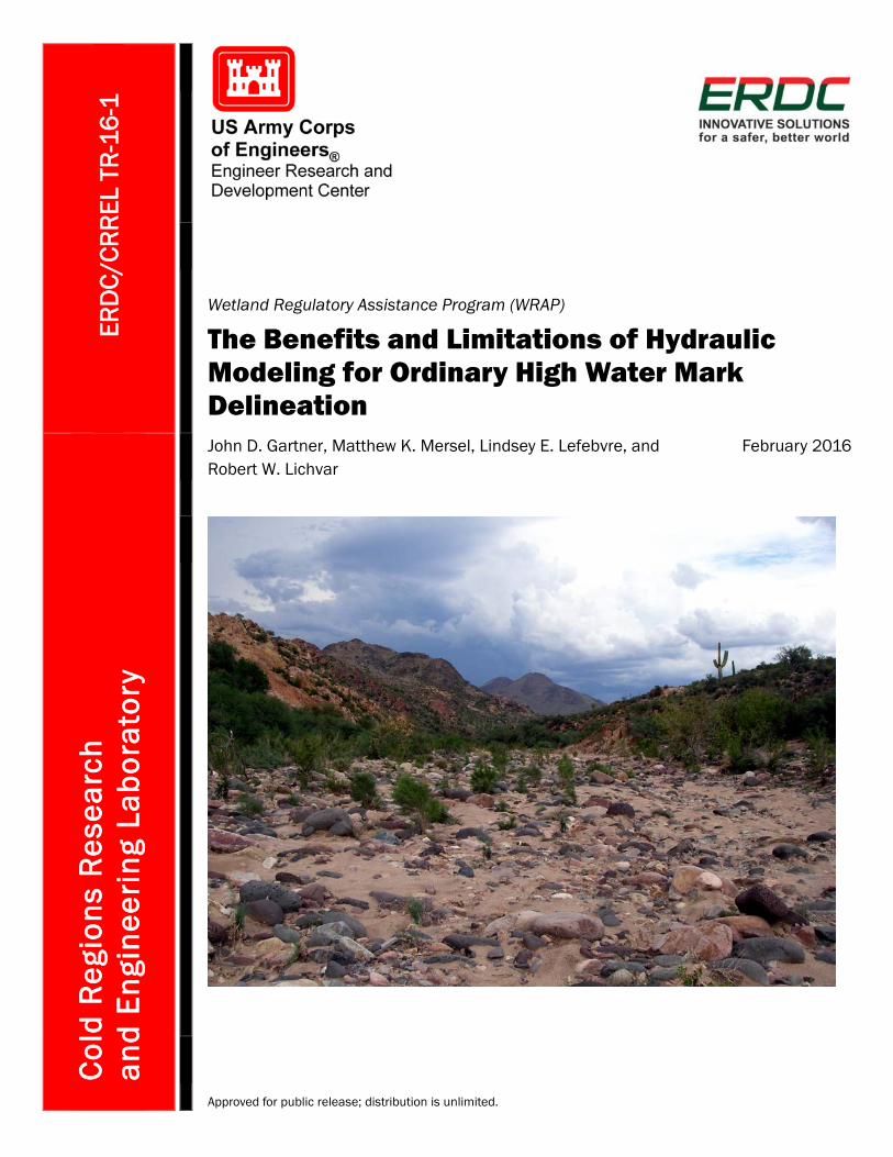
Cover image: New River near Rock Springs, AZ. The river had been dry for 15 months at the time of the photo, but the storms clouds pictured in the background helped produce a small flow event later that evening.

The U.S. Army Engineer Research and Development Center (ERDC) solves the nation’s toughest engineering and environmental challenges. ERDC develops innovative solutions in civil and military engineering, geospatial sciences, water resources, and environmental sciences for the Army, the Department of Defense, civilian agencies, and our nation’s public good. Find out more at www.erdc.usace.army.mil.

To search for other technical reports published by ERDC, visit the ERDC online library at http://acwc.sdp.sirsi.net/client/default.

http://www.erdc.usace.army.mil/

http://acwc.sdp.sirsi.net/client/default

Wetland Regulatory Assistance Program (WRAP)

ERDC/CRREL TR-16-1 February 2016


John D. Gartner, Matthew K. Mersel, Lindsey E. Lefebvre, and Robert W. Lichvar U.S. Army Engineer Research and Development Center (ERDC) Cold Regions Research and Engineering Laboratory (CRREL) 72 Lyme Road Hanover, NH 03755-1290

Final Report

Approved for public release; distribution is unlimited.

Prepared for Headquarters, U.S. Army Corps of Engineers Washington, DC 20314-1000

Under Wetlands Regulatory Assistance Program (WRAP)

ERDC/CRREL TR-16-1 ii

Abstract

This document explores the use of hydraulic modeling for ordinary high water mark (OHWM) delineation as performed for the purposes of Clean Water Act implementation and other applications. OHWM delineation in streams and rivers is primarily based on field indicators, which can be challenging to interpret in these dynamic systems. Computational hydrau-lic modeling simulates the water surface elevation and width for a given discharge. This modeling can be helpful in OHWM delineations but can be misleading if the model assumptions are not met, the model inputs are not carefully chosen, or the error estimates of the model are unclear. This doc-ument demonstrates how hydraulic modeling can assist with OHWM de-lineation in rivers and streams and how modeling may be misused or mis-leading. Two separate companion documents focus on (a) flow frequency analysis and hydrologic modeling and (b) the combined use of hydraulic modeling and flow frequency analysis in OHWM delineation.

DISCLAIMER: The contents of this report are not to be used for advertising, publication, or promotional purposes. Ci-tation of trade names does not constitute an official endorsement or approval of the use of such commercial products. All product names and trademarks cited are the property of their respective owners. The findings of this report are not to be construed as an official Department of the Army position unless so designated by other authorized documents. DESTROY THIS REPORT WHEN NO LONGER NEEDED. DO NOT RETURN IT TO THE ORIGINATOR.

ERDC/CRREL TR-16-1 iii

Contents Abstract .......................................................................................................................................................... ii

Illustrations .................................................................................................................................................... iv

Preface ............................................................................................................................................................. v

Acronyms and Abbreviations ...................................................................................................................... vi

1 Introduction ............................................................................................................................................ 1 1.1 Background ..................................................................................................................... 1 1.2 Objectives ........................................................................................................................ 3 1.3 Approach ......................................................................................................................... 3

2 Modeling Background ......................................................................................................................... 5 2.1 Computational vs. physical modeling ............................................................................ 5 2.2 Hydrologic and hydraulic modeling ................................................................................ 6 2.3 1-D, 2-D, and 3-D hydraulic modeling ........................................................................... 7 2.4 Field validation .............................................................................................................. 10 2.5 Steady vs. unsteady flow .............................................................................................. 11 2.6 Subcritical vs. critical vs. supercritical flow ................................................................. 11 2.7 Channel geometry......................................................................................................... 12 2.8 Suitable models ............................................................................................................ 12

3 Manning Equation...............................................................................................................................13 3.1 Overview and parameters ............................................................................................ 13 3.1.1 Velocity .................................................................................................................................... 14 3.1.2 Unit conversion factor ............................................................................................................ 14 3.1.3 Roughness .............................................................................................................................. 14 3.1.4 Hydraulic radius ..................................................................................................................... 16 3.1.5 Friction slope .......................................................................................................................... 16

3.2 Manning equation example .......................................................................................... 17 3.3 Uncertainties in the Manning equation and modeling in general.............................. 19

4 HEC-RAS Modeling ............................................................................................................................. 21 4.1 Overview ........................................................................................................................ 21 4.2 Model inputs and output uncertainty .......................................................................... 22 4.2.1 Cross-section data .................................................................................................................. 22 4.2.2 Roughness .............................................................................................................................. 25 4.2.3 Boundary conditions .............................................................................................................. 26 4.2.4 Multiple channels and ineffective or unconnected flow areas ............................................ 27 4.2.5 Discharge ................................................................................................................................ 28

4.3 Model assumptions and other considerations ........................................................... 30

5 HEC-GeoRAS ........................................................................................................................................ 32

6 Summary ............................................................................................................................................... 36

References ................................................................................................................................................... 37

Report Documentation Page

ERDC/CRREL TR-16-1 iv

Illustrations

Figures

1 A physical model (also called a scale model) of the Ohio River constructed by the U.S. Army Corps of Engineers (Fatheree 2006) ......................................................................... 5

2 An example of computational hydraulic modeling to assist in OHWM delineation: an X-Y-Z perspective plot of a one-dimensional HEC-RAS hydraulic model of Mission Creek near Desert Hot Springs, CA ............................................................................... 7

3 An example of a 2-D hydraulic model to simulate flow extent, direction, and velocity at St Mary’s City, MD (Donnell 2009) ............................................................................ 9

4 A cross-sectional view of Cristianitos Creek, San Clemente, CA, showing flow modeling using the Manning equation ...................................................................................... 18

5 A comparison of cross-section survey strategies: (A) true ground topography; (B) variable spacing of survey points; and (C) even spacing of survey points ............................ 23

6 The effect of altering cross-section spacing in HEC-RAS model runs at New River near Rock Springs, AZ .................................................................................................................. 24

7 The effect of altering n values on modeled water surface elevations at New River near Rock Springs, AZ .................................................................................................................. 25

8 The effect of altering boundary conditions on modeled water surface elevations at New River near Rock Springs, AZ ........................................................................................... 27

9 The effect of multiple channels on the simulated water surface of a 10-year recurrence-interval flow at Mission Creek near Desert Hot Springs, CA .............................. 28

10 A HEC-RAS simulation of multiple flows to determine discharges associated with various points of interest in an OHWM delineation at the New River near Rock Springs, AZ ..................................................................................................................................... 29

11 A HEC-GeoRAS simulation of water depth and extent of the 5-, 10-, and 25-year return interval discharges at Mission Creek near Desert Hot Springs, CA (Lichvar et al. 2006.) ................................................................................................................................... 34

12 HEC-GeoRAS and HEC-RAS models of a 2-year recurrence-interval flow at Mink Brook in Hanover, NH ................................................................................................................... 35

Tables

1 Representative values of n, Manning’s coefficient of roughness (Brunner 2010a) ........... 15

ERDC/CRREL TR-16-1 v

Preface

Support and funding for this project were provided by the U.S. Army Corps of Engineers (USACE) Headquarters through the Wetlands Regula-tory Assistance Program (WRAP). The authors acknowledge and appreci-ate the interest and support of Margaret Gaffney-Smith, Jennifer Moyer, Karen Mulligan, and Stacey Jensen of the USACE Headquarters Regula-tory Program and Sally Stroupe of the USACE Engineer Research and De-velopment Center (ERDC) Environmental Laboratory.

This report was prepared by John D. Gartner, Matthew K. Mersel, Lindsey E. Lefebvre, and Robert W. Lichvar (LiDAR and Wetlands Group, David Finnegan, Chief), USACE ERDC Cold Regions Research and Engineering Laboratory (CRREL). At the time of publication, Timothy Pangburn was Director of the Remote Sensing and Geographic Information Systems Cen-ter of Expertise (RS/GIS CX), ERDC-CRREL. The Deputy Director of ERDC-CRREL was Dr. Lance Hansen, and the Director was Dr. Robert Davis.

The authors thank Dr. Steven Daly of ERDC-CRREL and Aaron Damrill of the USACE Detroit District for their thoughtful and insightful reviews.

COL Bryan S. Green was the Commander of ERDC, and Dr. Jeffery P. Hol-land was the Director.

ERDC/CRREL TR-16-1 vi

Acronyms and Abbreviations

1-D 1-Dimensional

2-D 2-Dimensional

3-D 3-Dimensional

CRREL U.S. Army Cold Regions Research and Engineering Laboratory

CWA Clean Water Act

DEM Digital Elevation Model

ERDC Engineer Research and Development Center

FEMA Federal Emergency Management Agency

GIS Geographic Information System

GPS Global Positioning System

HEC-RAS Hydraulic Engineering Center River Analysis System

LiDAR Light Detection and Ranging

OHWM Ordinary High Water Mark

RS/GIS Remote Sensing and Geographic Information Systems

SMS Surface Water Modeling System

USACE U.S. Army Corps of Engineers

USGS U.S. Geological Survey

WRAP Wetland Regulatory Assistance Program

ERDC/CRREL TR-16-1 1

1 Introduction

1.1 Background

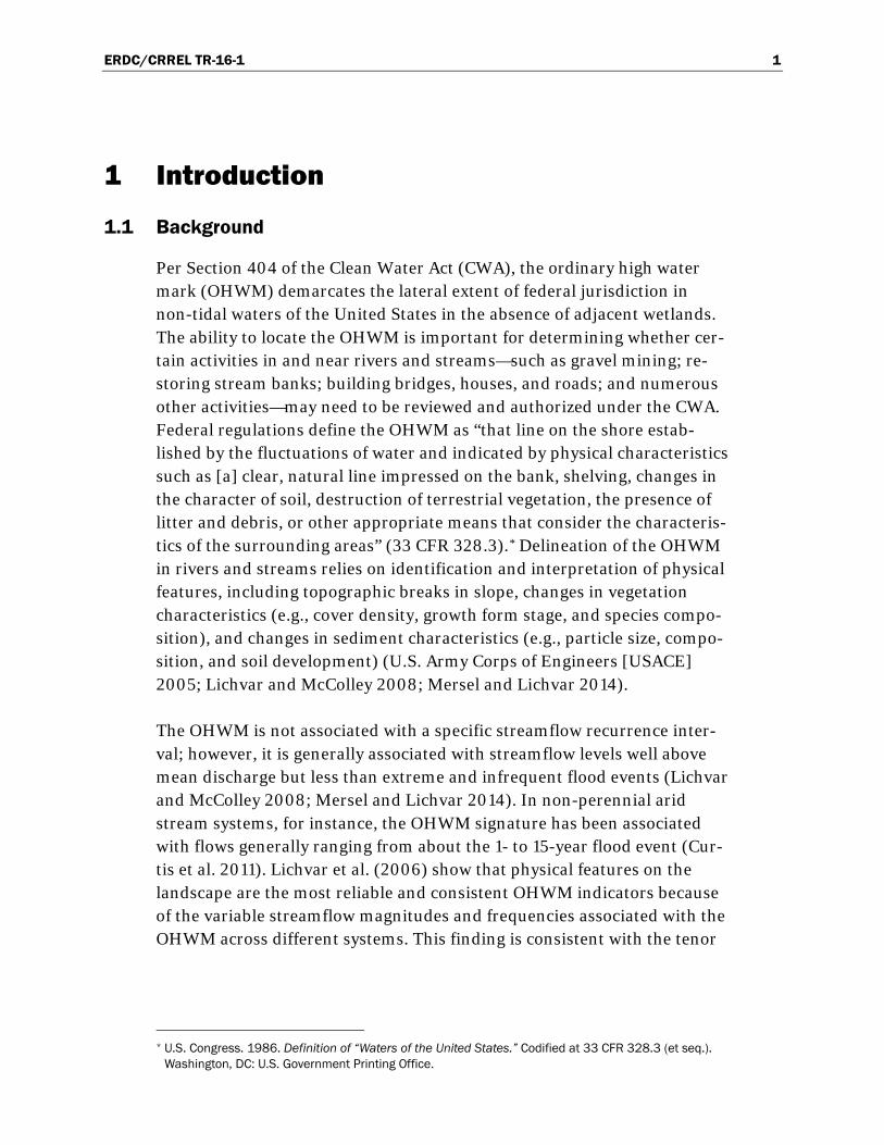
Per Section 404 of the Clean Water Act (CWA), the ordinary high water mark (OHWM) demarcates the lateral extent of federal jurisdiction in non-tidal waters of the United States in the absence of adjacent wetlands. The ability to locate the OHWM is important for determining whether cer-tain activities in and near rivers and streams—such as gravel mining; re-storing stream banks; building bridges, houses, and roads; and numerous other activities—may need to be reviewed and authorized under the CWA. Federal regulations define the OHWM as “that line on the shore estab-lished by the fluctuations of water and indicated by physical characteristics such as [a] clear, natural line impressed on the bank, shelving, changes in the character of soil, destruction of terrestrial vegetation, the presence of litter and debris, or other appropriate means that consider the characteris-tics of the surrounding areas” (33 CFR 328.3).* Delineation of the OHWM in rivers and streams relies on identification and interpretation of physical features, including topographic breaks in slope, changes in vegetation characteristics (e.g., cover density, growth form stage, and species compo-sition), and changes in sediment characteristics (e.g., particle size, compo-sition, and soil development) (U.S. Army Corps of Engineers [USACE] 2005; Lichvar and McColley 2008; Mersel and Lichvar 2014).

The OHWM is not associated with a specific streamflow recurrence inter-val; however, it is generally associated with streamflow levels well above mean discharge but less than extreme and infrequent flood events (Lichvar and McColley 2008; Mersel and Lichvar 2014). In non-perennial arid stream systems, for instance, the OHWM signature has been associated with flows generally ranging from about the 1- to 15-year flood event (Cur-tis et al. 2011). Lichvar et al. (2006) show that physical features on the landscape are the most reliable and consistent OHWM indicators because of the variable streamflow magnitudes and frequencies associated with the OHWM across different systems. This finding is consistent with the tenor

* U.S. Congress. 1986. Definition of “Waters of the United States.” Codified at 33 CFR 328.3 (et seq.).

Washington, DC: U.S. Government Printing Office.


of the federal OHWM definition, which emphasizes physical features as defining criteria.

However, delineating the OHWM based on visual observations alone can be challenging in some circumstances. It is usually difficult if not impossi-ble to know the flow amount or recurrence interval associated with various physical features without analysis beyond field reconnaissance. Moreover, it may be difficult to interpolate the OHWM between widely spaced field indicators; and it may be unclear if a physical feature on one side of a wa-terway is associated with the same flow level as a physical feature on the other side of the channel.

By simulating the elevation and lateral extent of a given flow in a given channel geometry, hydraulic modeling can assist with these and other dif-ficulties pertaining to OHWM delineation (Figure 2). Simply put, through the use of hydraulic modeling, one does not need to observe a particular flow amount to understand the width and depth of that flow. With a hy-draulic model, a user can test if a physical feature or potential OHWM lo-cation corresponds with flow levels that are reasonably associated with the OHWM.

OHWM delineation can be a challenging procedure with many variables playing a role. Knowing the discharge amounts and frequencies associated with various field indicators can add to the preponderance of evidence that is needed for OHWM delineation, or it can help to rule out or confirm po-tential OHWM locations where field indicators are challenging to inter-pret. Indeed, hydraulic modeling can be so alluring that some attempts to delineate the OHWM have relied exclusively on the modeled extent of a certain flow event, such as the 2-year or 10-year recurrence-interval flow, even though this practice does not typically supplant the need for evidence of physical characteristics (USACE 2005).

Despite its benefits, hydraulic modeling can be misleading if performed or applied improperly; and agencies reviewing the models as part of a juris-dictional determination or permit application must understand the as-sumptions and limitations before relying on the output. For every project, a modeler makes explicit and implicit choices on the input data (e.g., cross-section spacing and boundary conditions), on the calculations (e.g., using equations for critical or subcritical flow regime), and on the accuracy (e.g., whether the flow extents are accurate on the scale of a meter or tens


of meters). The explicit choices can be difficult to identify depending on model complexity, and the implicit choices can be even harder to tease out. Typically, user manuals for these models focus on how to make the models produce an output but do not address the models’ applicability and limita-tions. Both the practitioners who create hydraulic models and the agencies that review them need to be aware of when, where, and how modeling can assist in OHWM delineation and when it falls short.

1.2 Objectives

This document focuses on the potential uses of hydraulic modeling in OHWM delineation and aims to provide modelers and reviewers with as-sistance beyond that available in user manuals. The intention is not to take the place of the specific manuals, training, and experience required to pro-ficiently use hydraulic modeling but instead to illustrate the importance and effects of choices made in hydraulic modeling as it applies to OHWM delineation.

1.3 Approach

First, this document provides an overview of hydraulic modeling in gen-eral and the wide range of available models. Next, special attention is given to (a) the Manning equation, because it is well established and rela-tively simple; (b) the Hydraulic Engineering Center River Analysis System (HEC-RAS), because it is a free and widely used hydraulic modeling pro-gram; and (c) HEC-GeoRAS, because it enhances visualization of the OHWM in concert with digital elevation models (DEMs) and remotely sensed imagery and allows interpolation of model results between sur-veyed cross sections. Through tests at field sites mostly in the arid and semi-arid areas of the southwestern U.S., this study examines and summa-rizes hydraulic modeling successes, requirements, limitations, and com-mon pitfalls.

Two companion documents focus on (a) flow frequency analysis, which can help to determine the frequency of various flow amounts and can be used in conjunction with hydraulic modeling (Gartner et al. 2016a), and (b) case studies on combining hydraulic and flow frequency analysis to as-sist in OHWM delineation in rivers and streams (Gartner et al. 2016b).

A principal conclusion of this document is that hydraulic modeling can be extremely helpful in some OHWM delineation scenarios but is best used in


conjunction with field evidence under most circumstances. The OHWM is principally defined as a physical feature and, as such, should be tied to physical evidence where possible. However, models may help to interpret physical indicators or add supporting evidence to OHWM delineations; and they can be especially helpful in circumstances where OHWM indica-tors have been obscured (e.g., heavily disturbed systems) or are otherwise unclear or where field access is impracticable.


2 Modeling Background

The terms model and modeling have many uses in science and engineer-ing, and the terminology and differentiation between different types of models can be confusing. By definition, a model is a “mathematical or physical simulation of a field-size situation” (Novak et al. 2010).

The following sections discuss modeling terminology (Sections 2.1 through 2.3) and provide an overview of issues that are pertinent to most models (Sections 2.4 through 2.8). These issues are further explored in Sections 3 through 5 as they pertain to and can be illuminated by specific types of computational hydraulic modeling.

2.1 Computational vs. physical modeling

Within the scope of hydraulic modeling, a main distinction exists between physical and computational models. A physical model is a physical copy of an object, often built at a smaller scale. For example, USACE has built sev-eral physical models of rivers out of plaster, metal, sand, etc., to examine the hydraulic effects of inserting or removing locks and dams on dynamic waterways, such as the Ohio River (Figure 1). The term scale model is syn-onymous with physical model. Although fascinating, physical models are costly; and the questions they are designed to answer typically do not help with OHWM delineation. This document does not further discuss physical models.

Figure 1. A physical model (also called a scale model) of the Ohio River constructed by the U.S. Army Corps of Engineers (Fatheree 2006).


Unlike scale models, computational models can be quite useful for OHWM delineation; thus, they are the focus of this report. These models use a set of algebraic and differential equations based on fundamental physical pro-cesses, such as Newton’s laws of motion, or well-established empirical re-lations, such as the Manning formula. The models convert a measured or estimated input (e.g., geometry, discharge rate, or channel roughness) into an output (e.g., water elevation or flow velocity). These models usually have certain assumptions to simplify the calculations, for example, assum-ing that the discharge rate is constant over short time periods or that the water flows in only one direction. Civil engineers often use the terms nu-merical model, computational model, and mathematical model inter-changeably although slight distinctions exist (Novak et al. 2010).

2.2 Hydrologic and hydraulic modeling

Two types of mathematical modeling are especially pertinent to OHWM delineation, each with its benefits and limitations:

• Hydrologic modeling can be used to determine the amount of flow dis-charge at a given location for a given recurrence interval, and in this use it is one of several methods used in flow frequency analysis.

• Hydraulic modeling can be used to determine the elevation and lateral extent of water and other hydraulic parameters at a given location for a given discharge.

The scales of these two types of modeling differ. Hydrologic modeling of-ten has a basin-wide view because the conditions throughout a contrib-uting area can affect the amount of water delivered to the location of inter-est. Hydraulic modeling focuses on the reach scale (i.e., a given length of a river or stream), often taking the amount of water delivered to a reach as a given input and then simulating the hydraulic properties of the water as it flows through a reach. This document focuses on computational hydraulic modeling; a companion document focuses on hydrologic modeling and other types of flow frequency analysis (Gartner et al. 2016a).

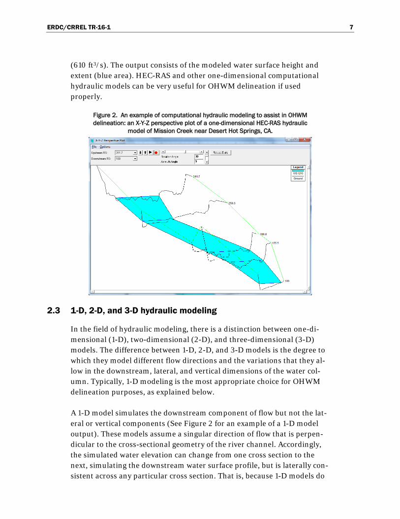
Figure 2 shows an example output of computational hydraulic modeling, in this case an X-Y-Z perspective plot from a one-dimensional HEC-RAS hydraulic model of Mission Creek near Desert Hot Springs, CA. The sur-veyed ground surface elevation at cross sections (black lines) is one of the key input parameters. Another input is the estimated discharge of an ap-proximately 10-year recurrence-interval flow event, in this case 17.3 m3/s


(610 ft3/s). The output consists of the modeled water surface height and extent (blue area). HEC-RAS and other one-dimensional computational hydraulic models can be very useful for OHWM delineation if used properly.

Figure 2. An example of computational hydraulic modeling to assist in OHWM delineation: an X-Y-Z perspective plot of a one-dimensional HEC-RAS hydraulic

model of Mission Creek near Desert Hot Springs, CA.

2.3 1-D, 2-D, and 3-D hydraulic modeling

In the field of hydraulic modeling, there is a distinction between one-di-mensional (1-D), two-dimensional (2-D), and three-dimensional (3-D) models. The difference between 1-D, 2-D, and 3-D models is the degree to which they model different flow directions and the variations that they al-low in the downstream, lateral, and vertical dimensions of the water col-umn. Typically, 1-D modeling is the most appropriate choice for OHWM delineation purposes, as explained below.

A 1-D model simulates the downstream component of flow but not the lat-eral or vertical components (See Figure 2 for an example of a 1-D model output). These models assume a singular direction of flow that is perpen-dicular to the cross-sectional geometry of the river channel. Accordingly, the simulated water elevation can change from one cross section to the next, simulating the downstream water surface profile, but is laterally con-sistent across any particular cross section. That is, because 1-D models do


not simulate water flowing horizontally, the modeled water elevation is the same on both sides of a river at any given cross section. Close inspection of a real river during a high water event indicates that the water elevation is often slightly higher on one side of the channel than the other, especially on the outside of a meander bend. Thus, a 1-D model has an inherent sim-plification of a river system and cannot exactly simulate the true water sur-face.

Several benefits come with this simplification. The data requirements for a 1-D model are reasonable—primarily cross-section surveys spaced tens to hundreds of meters apart or greater, depending on the channel form and geometry and the question at hand. Only one or two boundary conditions are required to be input into the model, and the boundary conditions are more easily established for 1-D models than for 2-D and 3-D models. The computations are relatively simple; and the entire modeling procedure, in-cluding field verification, can be fairly rapid and inexpensive. For decades, floodplain management and flood insurance studies have used 1-D hy-draulic models of riverways to simulate floodwater elevations.

A 2-D model simulates the downstream and lateral components of flow, but not the vertical component—water is modeled to flow downstream and left and right, but not up and down. With 2-D modeling, the simulated wa-ter surface can be higher on one side of the channel than on the other, which might better reflect real-world conditions. A 2-D model can also simulate eddies and recirculating flow. They have been used to simulate highly varied flows at levee breaks and water velocities downstream of dams to optimize fish release locations. Additionally, 2-D modeling can be helpful in complicated urban areas and for broad floodplains that are greater than three times the channel width (Néelz and Pender 2009). For example, Figure 3 shows the non-parallel flow paths though a complicated channel at St Mary’s, MD, modeled in the Surface Water Modeling System (SMS), a model developed by USACE. Note that for OHWM delineation purposes, the area of interest is typically not far out onto wide floodplains but instead near the channel edge and at low floodplain surfaces.

In rare situations, a 2-D model might be preferable to a 1-D model for OHWM delineation purposes (Chow et al. 1988; WRC Engineering, Inc. 2008). In locations where the hydraulics are complicated by many physi-cal features in the water, such as multiple bridge crossings or dilapidated


levee systems, a detailed survey would be needed to make any model rep-resentative of water surfaces in the system; and the 2-D model setup might be easier than the calibration needed for a 1-D model. The uses of 2-D models might also be beneficial at locations where the water elevations are much higher on one side of the channel than the other, such as at a sharp bend.

Figure 3. An example of a 2-D hydraulic model to simulate flow extent, direction, and velocity at St Mary’s City, MD (Donnell 2009).

Generally, 2-D modeling is reserved for hydraulic analyses that go beyond the typical OHWM-related queries about water elevation and extent. 2-D models have greater data requirements, typically a mesh or gridded survey rather than the more widely spaced cross sections required for 1-D hydrau-lic modeling. They require more boundary conditions, which are slightly harder to establish. They also require more time for model setup and veri-fication and a higher level of engineering expertise.

3-D models simulate the downstream, lateral, and vertical components of flow. The vertical changes in hydraulics that 3-D modeling simulates are generally not pertinent to OHWM delineation. 3-D modeling has been used on rivers to investigate flow velocities and forces in specific locations, such as at a drop weir structure or a single lock and dam. More commonly, though, 3-D hydraulic modeling is used in industrial applications, such as modeling the flow in a turbine or hydraulic manifold.

In sum, 1-D modeling has reasonable data requirements and a long-stand-ing record of use in simulating water elevations. The marginal improve-ments, if any, in 2-D and 3-D modeling of water elevations do not merit


the additional survey requirements, the greater difficulty in model setup and verification, the additional engineering expertise, and the greater diffi-culty for regulators in reviewing the models. Therefore, this document fo-cuses on 1-D computational modeling.

2.4 Field validation

All models benefit from field validation, the exact method of which will vary from site to site. Sometimes, field validation can be strictly organized and systematic, for example, verifying that the simulated flow depth is within a certain percentage of the known flow depth for a given discharge. The known flow depth could be derived from measurements of water ele-vation at the time of the flow event, from watermarks of a recent storm event, or from the stage–discharge relationship developed at a stream gage.

Sometimes the field validation can be less systematic but still provide con-fidence (or lack thereof) in the model results. For example, a flow with a 0.1-year recurrence interval (a low flow that occurs, on average, approxi-mately 10 times per year) should not inundate a high floodplain in the model results, nor should the modeled 100-year recurrence interval flow be contained within the bottom confines of the channel. In this example, the model validation benefits from some knowledge of geomorphic princi-ples, such as the relationship between bankfull discharge and flow recur-rence intervals (Williams 1978).

Careful investigation of isolated areas is one of the most important aspects of ground truthing in hydraulic modeling. For example, a low area may be separated from the main channel by a high levee. There may be a connec-tion between these two areas upstream, or they may be isolated. The deci-sion to include or exclude this alternate channel can greatly influence the elevation and extent of modeled water surface profiles, and this decision must be verified by field observations and surveys. Section 4 on HEC-RAS modeling addresses this concept further (e.g., Figure 9).

At a minimum, a flow estimate should be made at the time of the cross-section surveys, and this can be used to help calibrate a model and to vali-date the modeled water surface elevations. The validation may or may not be entirely appropriate for higher flows, but it is better than no validation at all.


2.5 Steady vs. unsteady flow

Steady flow has a constant discharge rate over time, and unsteady flow has a changing discharge over time. The time period of analysis affects whether flow is characterized as steady or unsteady. Over the course of a minute, river flows generally do not change much and can be assumed steady. However, the change in flows during a flood can be characterized as unsteady, especially in arid regions where the flood hydrographs can rise and fall rapidly. Many computational hydraulic models assume steady flow because it greatly simplifies the physics and math of the simulation.

Generally, steady-flow hydraulic modeling is sufficient when modeling is used to assist in OHWM delineation. Unsteady-flow hydraulic modeling and its added complications are not typically required to assist in OHWM delineation because the unsteadiness of flow generally does not greatly af-fect stage calculations. Water levels from stage calculations are often the sought-after variable in hydraulic modeling for OHWM purposes.

2.6 Subcritical vs. critical vs. supercritical flow

Although these are specialized hydraulic terms, they characterize an im-portant trait of water in natural channels. Subcritical flow describes water velocity that is less than the velocity of a wave traveling through the water. For example, if someone were to make a splash in the water, the waves would travel in all directions, including upstream. In this situation, imped-ances to flow can affect the hydraulics at upstream locations.

Supercritical flow describes water velocity that is greater than the velocity of a wave traveling through the water. An example would be in a chute or over a waterfall. If someone were to make a splash in the water, the wave on the water would be swept downstream faster than it could travel up-stream. In this situation, any impedance to flow has little or no effect on the hydraulics at upstream locations.

Critical flow occurs at the transition between supercritical and subcritical flows. In HEC-RAS modeling, different solution procedures are used to simulate subcritical and subcritical flow outputs, and the locations of criti-cal flow are clearly marked to show the transition in flow properties and the resulting shift in computational methods.


2.7 Channel geometry

All computational hydraulic modeling is based to some extent on the ge-ometry of the channel. This geometry can be surveyed by the traditional method using an auto level and measuring tape; or it can be obtained through more advanced instruments, such as a laser theodolite (also called a total station), real-time kinetic GPS (global positioning system), ground-based LiDAR (Light Detection and Ranging), or aerial LiDAR. In most cir-cumstances, topography from the U.S. Geological Survey (USGS) 7.5-mi-nute topographic maps or 10 m DEMs does not have a resolution sufficient for OHWM-related modeling. Often, surveying the underwater portions of a river or stream channel is most difficult, but this topography is critical for the accurate simulation of water surfaces.

A trade-off exists between survey resolution and time and cost. At each site, finding the right balance is a matter of professional judgment. Re-viewers of computational models should always consider whether the spa-tial resolution of the geometry data is appropriate for OHWM delineation.

Modeling alluvial fans and other dynamic, multi-threaded channels is es-pecially sensitive to survey resolution. Subtle levees can direct flow from one channel to another. It is possible that low-resolution DEMs (e.g., 10 m gridding) and low-resolution surveys may not pick up these low-relief in-fluences on flow. Section 4 provides examples to further demonstrate the effects of survey resolution on HEC-RAS modeling.

2.8 Suitable models

Many hydraulic models are available. The Federal Emergency Manage-ment Agency (FEMA) publishes an online list of current nationally and lo-cally accepted hydraulic models for flood-hazard mapping (FEMA 2014), most of which would be suitable for assisting in OHWM delineation. As of August 2015, the national list included thirteen 1-D steady-flow models, ten 1-D unsteady-flow models, and six 2-D steady and unsteady models. Some of the most commonly used models are HEC-RAS, WSPRO, XP-SWMM, and MIKE. Additional useful models include SMS and the Man-ning equation. This document focuses on HEC-RAS, HEC-GeoRAS, and the Manning equation because they are well established, free, and com-monly used.


3 Manning Equation

3.1 Overview and parameters

Most hydrologists would consider the Manning equation to be a well-at-tested empirical relationship; but in its essence, it is a model. Using the in-put of slope, cross-section geometry, and roughness, the equation com-putes an output of water velocity or discharge. The importance for OHWM delineation is that the Manning equation computes the discharge for a given water elevation, and it can be rearranged to calculate the water ele-vation for a given discharge. Many questions pertinent to OHWM analysis can be answered using this formula; for example, determining the dis-charge associated with a physical feature that might be an OHWM field in-dicator.

The Manning equation is a fundamental aspect of hydraulic analysis. Un-derstanding it helps to understand more complicated models, such as HEC-RAS. Below describes the formula and some questions that the Man-ning equation might answer to assist in OHWM delineation.

The classic form of the equation is

𝑉𝑉 = 𝑘𝑘𝑛𝑛

𝑅𝑅ℎ2/3𝑆𝑆𝑓𝑓

1/2 (1)

where

V = velocity, K = a conversion factor for SI and U.S. customary units, n = Manning’s coefficient of roughness, Rh = hydraulic radius, and Sf = friction slope.

The hydraulic radius is computed by

𝑅𝑅ℎ = 𝐴𝐴/𝑃𝑃 (2)

where

A = channel flow area and P = wetted perimeter.


It is relatively easy to develop an intuitive sense of the elements of the Manning equation. For instance, water flowing down steep channels should flow faster than water flowing down channels of lesser incline. Ad-ditionally, if there is high roughness (n value) to the channel, it slows the water velocity.

The importance of the Manning equation for OHWM delineation is that it can be used to relate the elevation of the water surface to its discharge rate because discharge is simply the product of channel area and velocity:

𝑄𝑄 = 𝑉𝑉𝐴𝐴 = 𝐴𝐴 𝑘𝑘𝑛𝑛𝐴𝐴 𝑅𝑅ℎ

2/3𝑆𝑆𝑓𝑓1/2 (3)

where Q = discharge.

The individual elements of the Manning equation are discussed next.

3.1.1 Velocity

Velocity, V, is the average velocity of the water flowing downstream. The equation gives just one velocity—it accounts for no variation from one side of the channel to the other or from the bottom of the water column to the surface. However, users might divide the channel into lateral sections and use the Manning equation for each section individually. Often, modelers compute an average velocity for the left overbank area, the main channel, and the right overbank area separately.

3.1.2 Unit conversion factor

The conversion factor, k, is included simply to keep the units in order. The value is 1 m1/3 s−1 for SI units and 1.4859 ft1/3 s−1 for U.S. customary units.

3.1.3 Roughness

Roughness, n, is one element that may be difficult for uninitiated users. In concept, the average downstream velocities are slower in rough channels, such as when there is dense vegetation in the flow path or large protruding rocks in the channel. Table 1 shows common values for various settings. Users can pick the appropriate n value from tables and illustrated manu-als, many of which are available online (Brunner 2010a; Barnes 1987; USGS 2014), or compute n values from a known channel geometry and set of flows at a site. The roughness can be the next order of magnitude higher


when the flow encounters brush, willows, or heavy stands of timber. For this reason, overbank flow velocities outside of the main channel are often calculated separately from the main channel velocities; and different n val-ues can be assigned to different zones of flow.

For most natural channels, the values in Table 1 do not have an extremely large range and are within the same order of magnitude: about 0.03 to 0.08. Thus, picking an incorrect n value will often result in a relatively mi-nor miscalculation of velocity and water surface elevation, as shown below in Section 4.2.2. Manning’s n can be a red herring—many reviewers of models focus on the chosen n value because it can be easily tweaked. Measurements of channel geometry tend to introduce more error than the n value, but it is harder to resurvey than to adjust the n value. If the chan-nel geometry is precisely and accurately measured, then roughness is the primary source of error in the Manning equation (Pappenberger et al. 2005). However, surveys of channel hydraulic radius and slope are inher-ently imperfect, they require professional judgment to set up, and they may be even larger sources of error than roughness in the Manning equa-tion.

Table 1. Representative values of n, Manning’s coefficient of roughness (Brunner 2010a, Table 3-1).


3.1.4 Hydraulic radius

Hydraulic radius, Rh, is defined as the ratio of a channel’s cross-sectional area of flow to its wetted perimeter (the “wet” portion of a cross section). This variable characterizes how much of the flow area is affected by the roughness on the bed and banks. Because it is the ratio of A over P, it rep-resents the relative importance of the downstream gravitational force, which acts over the entire area of the flow, versus the frictional force, which acts only on the perimeter of the flow. To gain an intuitive sense of this variable, consider two flows in channels of the same width, slope, and n value, where one channel has deep flow and the other has very shallow flow. The shallow flow has a lesser hydraulic radius than the deeper flow and, according to the Manning equation, should have a lower velocity than the deeper flow. It makes sense that the water flow is slower when it is shallow because it is influenced more by the roughness of the channel. To gain an intuitive sense of the Manning equation, hydraulic radius can be thought of loosely as the water depth; but this loose thinking can be mis-leading in some flow situations. For example, if the flow becomes high enough to spill onto the floodplain, Rh can stay constant or even decrease as water rises and becomes deeper, depending on the ratio of A to P as a function of stage.

There is a high level of professional judgment that goes into this parameter by way of choosing the location of the measured cross section. This cross section should be representative of the channel, it should be perpendicular to the flow direction, and it should not be in a location of rapidly changing width or slope where there is cross-channel flow or where the flow is tran-sitioning between critical and subcritical flow. Once the appropriate cross section is chosen, this variable is relatively easy to measure by surveying.

3.1.5 Friction slope

Friction slope, Sf, refers to the slope of the hydraulic grade line, which is equal to the water slope in uniform flow. Although flows are seldom per-fectly uniform, the friction slope can be approximated by the slope of the water surface if the channel geometry is not changing rapidly upstream or downstream.

Slope is generally the most difficult parameter to characterize correctly. In natural rivers, slope can vary over orders of magnitude between rivers and sometimes even on a single river from one reach to the next. Measuring


slope can be difficult because often one has to accurately measure a verti-cal change of less than a foot over a distance of hundreds or thousands of feet. Furthermore, the slope that should be measured is the slope at the time of the discharge in question, but it is unlikely that field measure-ments are made at the moment of this flow. This slope could differ sub-stantially from the channel bed slope or water surface slope at a different discharge, and using the bed slope or a low-discharge water surface slope is often not defensible.

A suitable method for estimating water surface slope is to measure the slope of high water marks of a recent flow event that is similar to the ex-pected elevation of the OHWM. These high water marks from a specific re-cent storm should not be confused with the ordinary high water mark, which is not indicative of a single flow. A high or moderate flow event will likely leave high water marks in the form of organic debris that accumu-lates at the highest water elevation on the bank. Matted vegetation, fine sediment deposits, and numerous other indicators are also indicative of high water marks. The slope of these high water marks from upstream to downstream locations can provide insight into the water surface slope at the moderate to high flows that are being analyzed for OHWM concerns.

If there are no clear high water marks, then slope can be measured from the water slope at the time of measurement, from the channel bed slope if it is not extremely undulating in riffles and pools, or from contour lines on 7.5-minute USGS topographic maps. In the best-case scenario, all of these measurements are roughly similar, which would lend more confidence to the slope input to the model.

3.2 Manning equation example

The following example illustrates how this equation can assist in OHWM delineation.

On Cristianitos Creek in San Clemente, CA (Figure 4), there are two eleva-tions that might be suitable OHWM locations based on physical indicators. At the elevation of 29.9 m, there is a break in slope at the top of an inset channel and a slight change in sediment texture, indicated by sand, gravel, and cobble transitioning to only sand and gravel. At a higher elevation, 31.1 m, there is another break in slope on the right bank, which is accom-


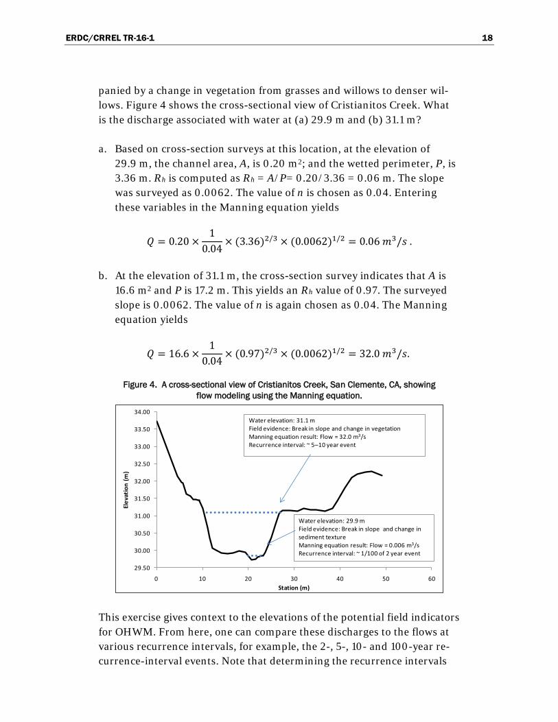
panied by a change in vegetation from grasses and willows to denser wil-lows. Figure 4 shows the cross-sectional view of Cristianitos Creek. What is the discharge associated with water at (a) 29.9 m and (b) 31.1 m?

a. Based on cross-section surveys at this location, at the elevation of 29.9 m, the channel area, A, is 0.20 m2; and the wetted perimeter, P, is 3.36 m. Rh is computed as Rh = A/P= 0.20/3.36 = 0.06 m. The slope was surveyed as 0.0062. The value of n is chosen as 0.04. Entering these variables in the Manning equation yields

𝑄𝑄 = 0.20 ×1

0.04× (3.36)2/3 × (0.0062)1/2 = 0.06 𝑚𝑚3/𝑠𝑠 .

b. At the elevation of 31.1 m, the cross-section survey indicates that A is 16.6 m2 and P is 17.2 m. This yields an Rh value of 0.97. The surveyed slope is 0.0062. The value of n is again chosen as 0.04. The Manning equation yields

𝑄𝑄 = 16.6 ×1

0.04× (0.97)2/3 × (0.0062)1/2 = 32.0 𝑚𝑚3/𝑠𝑠.

Figure 4. A cross-sectional view of Cristianitos Creek, San Clemente, CA, showing flow modeling using the Manning equation.

This exercise gives context to the elevations of the potential field indicators for OHWM. From here, one can compare these discharges to the flows at various recurrence intervals, for example, the 2-, 5-, 10- and 100-year re-currence-interval events. Note that determining the recurrence intervals

29.50

30.00

30.50

31.00

31.50

32.00

32.50

33.00

33.50

34.00

0 10 20 30 40 50 60

Elev

atio

n (m

)

Station (m)

Water elevation: 31.1 mField evidence: Break in slope and change in vegetationManning equation result: Flow = 32.0 m3/sRecurrence interval: ~ 5–10 year event

Water elevation: 29.9 mField evidence: Break in slope and change in sediment textureManning equation result: Flow = 0.006 m3/s Recurrence interval: ~ 1/100 of 2 year event


requires gage analysis, regional regression equations, or hydrologic model-ing, which are covered in a companion document (Gartner et al. 2016a).

In this case, the lower flow of 0.06 m3/s (2.1 ft3/s) is on the order of 1/100 of the 2-year recurrence-interval flow of about 5.5 m3/s (about 200 ft3/s). The higher flow of 32.0 m3/s (1130 ft3/s) corresponds with the 5- to 10-year recurrence-interval flow, which is in a much more reasonable range for the OHWM (Lichvar et al. 2006; Curtis et al. 2011). This analysis al-lows the investigator to rule out the lower of the two possible OHWM loca-tions.

3.3 Uncertainties in the Manning equation and modeling in general

More analysis of this example can verify how sensitive the calculations are to the n value. With an n value of 0.03, which is interpreted as the lowest reasonable value for this channel based on reference values in Table 1, the discharge in part b would be 42.6 m3/s (1500 ft3/s). If one enters what is interpreted as the highest reasonable value for n, 0.05, then the discharge would be 25.6 m3/s (900 ft3/s). These values are within approximately 35% of the originally computed discharge of 32.0 m3/s (1130 ft3/s). Section 4 on HEC-RAS modeling further explores the sensitivity of hydraulic mod-eling results to chosen n values (e.g., Figure 7).

In addition to the n value, it is possible to examine how different slope val-ues affect the computed discharge. The slope is computed as rise over run. For run, the distance between two surveyed height measurements should be measured along the curvilinear flow path. But many choices exist for determining the amount of rise. First, a survey of the thalweg (the deepest part of the channel) for 200 m upstream and downstream of the cross sec-tion yields a slope of 0.0062. This is the slope used in the Manning equa-tion in the above example because this creek lacked dramatic undulations from pools and riffles. Second, high water marks (higher than the eleva-tion for flow in part b) expressed downstream slopes ranging from 0.0065 to 0.0029. Third, the slope of the creek measured on a 7.5-minute USGS topographic map was 0.0036. Although there is discrepancy in these slope values, they are all in the same order of magnitude, which lends some con-fidence that the true slope is near this range. Using these various slopes in the Manning equation, it was found that discharges for part b ranged from 21.9 to 32.0 m3/s (770 to 1130 ft3/s), which is within approximately 35% of the originally computed discharge.


The uncertainty in this example due to uncertainty in slope and Manning’s n is substantial but much less than the variability of flow in this stream, which spans several orders of magnitude. Moreover, the uncertainty is much less than the difference between the flows computed in part a and part b. Thus, even though the flow computations are not perfect, they are adequate to help answer the question at hand and to provide meaningful insight into which elevation is most suitable for delineating the OHWM.

In any modeling exercise, the computations yield an estimate of discharge, not the actual discharge. Even direct flow measurements using a flow me-ter or a weir have associated error—in best-case scenarios, the error is less than 10%. Indirect methods of measuring discharge, such as the Manning equation, often have an associated error of 30% or more, simply because of uncertainties in measuring the slope, channel geometry, and roughness. Fortunately, typical flow estimates using the Manning equation are not or-ders of magnitude different than actual discharge, yet discharge does vary by orders of magnitude in hydrologically unregulated waterways. Thus, the Manning equation can help constrain or bracket the flow amount. Users and reviewers of the Manning equation should be aware of this limitation.

Herein lies an essence of field science and engineering—the measurements and modeling efforts never yield an exact or complete answer, but the quantitative results improve understanding of the investigated system. In this example, knowing the discharge amounts advances the question of which of these two locations is more reasonable for OHWM delineation. At the same time, the quantitative values risk giving a false sense of accuracy and precision. Users and reviewers should be aware of the accuracy of the results either in a formal error analysis or in a more general appreciation for the potential errors. Moreover, users and reviewers must acknowledge whether a quantitative estimate of the discharge completely answers the question of where the OHWM is located. In this example, it advances but does not fully answer this question.

The exact location of the OHWM cannot be determined by the Manning equation or by any other hydraulic model alone. Typically, people will con-sider the hydraulic modeling analysis that relates discharge to water sur-face elevation and flow frequency analysis to estimate flow recurrence in-tervals. Then all of the results are summed with field indicators and professional judgment to delineate the OHWM.


4 HEC-RAS Modeling

4.1 Overview

HEC-RAS is a 1-D computational model that simulates the hydraulics of water flow through natural rivers and other channels. USACE developed the model and provides extensive documentation (Brunner 2010a, 2010b) and regular enhancements to the program. This program is free and is widely used in government agencies and private firms by scientists and en-gineers versed in hydraulic analysis. Because the Manning equation is one of the core equations in the HEC-RAS computations, the preceding section on the Manning equation helps with comprehending the functions, ap-plicability, and limitations of HEC-RAS modeling.

HEC-RAS can assist in OHWM delineation in numerous ways. The model-ing can simulate the water surface elevation for a given discharge or can allow a user to find the discharge that matches a given elevation. Once a model is set up for a given river reach, water surface profiles can be quickly modeled for a range of flows. In this way, a user can determine, for instance, the flow rate that would reach the level of field indicators or po-tential OHWM locations. The user can then combine these results with hy-drologic information (e.g., stream-gage information or modeled stream flow estimates) to determine the recurrence interval of a given discharge and to test if these flows are reasonable for the OHWM.

The required inputs for a HEC-RAS model are

• channel geometry in the form of a series of cross sections; • Manning’s roughness coefficient, n; • flow rates; • flow change locations (longitudinally along a river reach); and • boundary conditions, which are often the water surface slope or eleva-

tion at the downstream-most cross section.

Many outputs are available, such as water velocity and shear stress; but for OHWM delineation purposes, the most important outputs are typically the water elevation and water edge at each cross section.

When calculating the water surface profile for a given discharge through a reach, HEC-RAS operates by computing the 1-D energy equation if flow is


subcritical or the momentum equation if flow is supercritical. In the basic form, the model uses the water surface elevation at the downstream-most cross section as an initial input (i.e., the boundary condition) and uses the Manning equation in solving for the slope, and hence the water surface el-evation, to the next upstream cross section. It performs this iteratively up-stream through the study reach. The HEC-RAS reference manual (Brunner 2010a) provides a thorough explanation of the computations in the model.

In the process of building a HEC-RAS model, users must depend on pro-fessional judgment in making many choices about the data collection and analysis at each site. There is no set prescription for every location. Train-ing and experience are required to properly simulate the flows at a site, even when making use of the HEC-RAS user manuals and program docu-mentation. This information presented here does not supplant this train-ing and experience, nor the user manuals and documentation, but instead is designed to illustrate the importance and effects of the choices made in model development.

4.2 Model inputs and output uncertainty

The following sections lay out the essential considerations in making a HEC-RAS model and provide examples of how different decisions affect the modeled results in case studies on rivers in semi-arid, southwestern U.S. settings and in temperate locations in New England.

4.2.1 Cross-section data

The geometry of the waterway is one of the most important inputs of a HEC-RAS model, so surveys of the geometry require careful consideration. The extent and resolution of cross-section measurements determine the extent and resolution of the HEC-RAS simulation. The surveys must span the entire reach in question, and the cross sections must extend laterally far enough to capture the elevation of the OHWM and any other features of interest. It is desirable to have additional cross sections beyond the reach in question, especially on the downstream end, to minimize the ef-fect of user-defined boundary conditions on the results at the area of inter-est (see Section 4.2.3 on boundary conditions).

The resolution of survey points along a cross section must be sufficient to capture the transitions in topography, especially in the vicinity of the OHWM elevation. It is generally preferable to have variable spacing of the


survey points to characterize breakpoints rather than an even spacing of survey points (Figure 5). Users should recognize that the variations in to-pography between survey points are not incorporated into the model. The exact number of survey points appropriate for a given cross section is a balance between the desire to have the most accurate model possible and the time and cost to survey many points.

Figure 5. A comparison of cross-section survey strategies: (A) true ground topography; (B) variable spacing of survey points; and (C) even spacing of

survey points.

Figure 5 shows an example of variable versus even spacing of survey points at a hypothetical cross section. Panels A through C show the true ground topography of the cross section (black line). Panel B shows a variable spac-ing of survey points (red dots) with the goal of characterizing the transi-tion points in topography. This survey portrays the major breaks in slope and shelving along the channel. Panel C shows an even spacing of the sur-vey points (blue dots). This method does not characterize several breaks in slope, some of which may be important for model accuracy and may be rel-evant to the OHWM location. In any case, survey points should be chosen carefully to capture the important changes along a cross section.

Likewise, the spacing and location of the cross sections longitudinally along a stream reach should characterize any significant changes in chan-nel geometry. Determining which changes are significant is a matter of


professional judgment. The considerations for choosing the spacing be-tween cross sections are similar to the considerations for choosing the ac-curacy of the survey along a cross section. There is a balance between reso-lution and the time and costs. Furthermore, from the standpoint of the HEC-RAS model, no variations in topography are “seen” between cross sections. For example, if there is an island between two cross sections, the HEC-RAS model will not show it. If there is a sudden drop in the channel, such as a waterfall or steep rapids, the hydraulic conditions at this drop will be interpolated between cross sections (Figure 6). Thus, the effects of this drop may be simulated over a greater channel length than they truly occur unless cross sections are situated just upstream and downstream of this drop.

Figure 6. The effect of altering cross-section spacing in HEC-RAS model runs at New River near Rock Springs, AZ.

Figure 6 illustrates an example where cross sections were removed from a HEC-RAS model at the location of a steep drop in the channel bed. The ef-fect on the modeled water surfaces is significant. The modeled flow is an approximately 2.8-year recurrence-interval event of 65 m3/s (3200 ft3/s) that occurred at this site on 26 December 2008. In the first run, six cross sections were input into the model (solid black line), and the resulting modeled water surface (solid blue line) reflects the effects of the steeper slope starting 100 m upstream. In the second run, only three cross sec-tions were included in the model, creating a smoother ground surface (dashed gray line, with “x” marks showing the removed cross sections). The resulting modeled water surface (blue dotted line) averages the effect of the steep drop over a greater channel length than it occurred.


Measurements of the reach lengths between cross sections are a potential source of error in a HEC-RAS model, but minimizing this error is not diffi-cult. Cross sections should be measured along the curvilinear flow paths, not straight lines, much as the slope should be measured along a curvilin-ear path in the Manning equation. Channel reach lengths are often meas-ured along the thalweg, which approximates the streamline of the bulk of the flow. Overbank reach lengths should be measured along the antici-pated path of the center of mass of the overbank flow (Brunner 2010b). Measuring reach lengths requires a proper interpretation of the landscape.

4.2.2 Roughness

HEC-RAS requires the user to define the roughness of channels and flood-plain surfaces. Different values can be input for the channel and overbank areas, which often have very different roughness values because of the abundance of vegetation on the overbank areas and the lack of vegetation in the main channel. Users generally input n, Manning’s roughness coeffi-cient. As with the Manning equation, HEC-RAS models are sensitive to the n value, especially for fine-tuning the models. However, given the rela-tively narrow range of n values in natural channels (see Table 1), entering incorrect n values does not typically lead to extreme errors in the model. Errors are generally less than 20%, as shown in the example in Figure 7. Although this error is not extreme, it can have an important effect in OHWM-related modeling in some circumstances. This roughness coeffi-cient can be calibrated based on field evidence of high water marks, sur-veys during flow events, and knowledge of stage–discharge relationships at stream gages.

Figure 7. The effect of altering n values on modeled water surface elevations at New River near Rock Springs, AZ.


Figure 7 shows how the chosen roughness value, n, can affect the modeled water surface elevation. In this example, using the same location and flow as in Figure 6, three HEC-RAS model runs show the effect of choosing high (0.05), moderate (0.04), and low (0.03) values for n. Higher rough-ness impedes the flow more; so with the higher n value, the water eleva-tions are higher than the other model runs to convey the same discharge amount. At most, the use of different n values changed the flow depth by approximately 20% in this example.

4.2.3 Boundary conditions

HEC-RAS requires only a downstream boundary condition in subcritical flow simulations, only an upstream boundary condition in supercritical flow simulations, and both downstream and upstream boundary condi-tions in mixed subcritical–supercritical flow simulations. The boundary condition can be based on a known water surface elevation, the critical wa-ter elevation for the modeled discharge, or a known slope. If a known slope is used, the energy gradient slope is the proper input although the water surface slope is often entered as an approximation of the energy gradient slope because the water surface slope can be measured in the field. In any case, the user-defined boundary condition has the greatest effect at the cross section where it is set; and the effect typically attenuates with dis-tance from the cross section, as illustrated below. For this reason, it desira-ble to have additional cross sections downstream of the reach of interest to minimize the effect of user-defined boundary conditions on this reach.

Figure 8 shows how boundary conditions can affect modeled water surface elevations in HEC-RAS but generally only in the most downstream of the modeled cross sections. This example again uses the same location and flow as in Figures 6 and 7. In the first run, the downstream boundary con-dition is established by the measured gage height. In the second run, the downstream boundary condition is established by the expected slope of the water surface. Note that the modeled flow elevation differs by up to about 0.6 m at the downstream end, but the difference is indistinguishable farther upstream. Because the potential errors generated by user-defined boundary conditions generally occur at only the downstream-most cross sections, it is best if the measured cross sections extend downstream of the reach of greatest interest.


Figure 8. The effect of altering boundary conditions on modeled water surface elevations at New River near Rock Springs, AZ.

4.2.4 Multiple channels and ineffective or unconnected flow areas

A user can define ineffective flow areas if there is no downstream trans-mission of water, for example, in an eddy immediately downstream of a bridge abutment. In a HEC-RAS output, these areas will be shown as inun-dated if the modeled water surface is higher than the ground surface; but the downstream velocity in these areas is considered nonexistent.

For example, in complicated channels and alluvial fans, as are often seen in arid and semi-arid environments, there might be side channels with no connection to the main channel. With multiple channels or depressions along a cross section, the user must consider if these are connected to the main channel or not. If the additional channels are not connected, they should be removed from the cross section. This requires examining the to-pography between cross sections and potentially far upstream of the study reach. Reviewers of HEC-RAS models with multiple channels or depres-sions should look for justification to include or exclude adjacent channels.

Figure 9 shows the effect of including or excluding adjacent channels in a semi-arid stream system. In this example, the additional channels to the left are sourced by a tributary that runs parallel to the main channel for 1000 m before connecting with the main channel 100 m downstream of this cross section. Panel A shows a HEC-RAS model that assumes that these channels are connected to the main flow channel even though they are not. In Panel B, the HEC-RAS model does not permit flow on the left side of the cross section unless the water levels overtop the high point be-tween the main channel and adjacent channels, reflecting field and aerial


image analysis that indicates the areas between stations 0 and 75 m are not connected to the main channel. There are substantial differences be-tween these two cases in the elevation and lateral extent of inundation. This example stresses the need for field verification of modeling results and for professional judgment in measuring cross sections, especially in tributary, distributary, and other multi-threaded channel systems.

Figure 9. The effect of multiple channels on the simulated water surface of a 10-year recurrence-interval flow at Mission Creek near Desert Hot Springs, CA.

Panel A shows the entire valley width with flows erroneously modeled in disconnected areas. Panel B shows only areas connected to upstream areas

and more accurately simulates the flow location, depth, and width.

4.2.5 Discharge

The flow to be modeled is also user defined; and, logically, higher flows typically equate to higher water surface elevations. The flow input into the model depends on the question at hand. For example, if a user wants to

0 20 40 60 80 100 120682.5

683.0

683.5

684.0

684.5

685.0

685.5

686.0

686.5

Mission_v3 xs A gage

Station (m)

Ele

vatio

n (m

)

Legend

WS Q10

Ground

0 20 40 60 80 100 120

683

684

685

686

Mission_v3 xs A gage

Station (m)

Ele

vatio

n (m

)

Legend

WS Q10

Ground

Bank Sta

main channeladjacent channelsA

B


know the elevation and extent of the water surface at the 5-year recur-rence-interval flow, then the first step would be to estimate this flow value and to use it as input. There can be substantial uncertainty in these flow-value estimates, which is a main focus of the companion document, Hy-drologic Modeling and Flood Frequency Analysis for Ordinary High Wa-ter Mark Delineation (Gartner et al. 2016a). If the user wants to determine the discharge required to inundate the channel up to a particular OHWM field indicator, then flow values can be entered iteratively until the water surface meets the field indicator (Figure 10).

Figure 10. A HEC-RAS simulation of multiple flows to determine discharges associated with various points of interest in an OHWM delineation at the New River near Rock Springs, AZ.

Figure 10 shows an example in which 11 flows were modeled to examine how these discharge amounts relate to various points of interest in an OHWM delineation. The lowest line corresponds to a recent peak annual flow of 3.9 m3 s−1 that occurred on the night of 21 August 2012 in between the two days that the team surveyed channel geometry. The middle set of lines spans two locations where notable changes in vegetation, sediment texture, and slope were surveyed in the field. The highest line simulates the discharge at the elevation of a high sand deposit from an extreme flood flow. The hydraulic modeling of flow elevations provides context to the field observations, especially when compared with flow recurrence inter-vals derived from flow frequency analysis.

HEC-RAS will model both steady and unsteady flow, but unsteady-flow simulations are generally not necessary for OHWM delineation purposes.


In a steady-flow simulation, HEC-RAS computes the hydraulics of a single flow value. Multiple flow values can be entered at once, and HEC-RAS will calculate the water surface of each flow independently. Unsteady-flow sim-ulations include a temporal component. For example, the water elevations over time can be computed through a network of channels over the course of a flood hydrograph. Unsteady-flow analysis can be more difficult than steady-flow analysis because instabilities can cause the program to fail to converge on a solution (Brunner 2010a). As noted above in Section 2.5, many users will specify steady flow if the simplification can be made be-cause adding variation in flow over time greatly increases the complexity of the computations.

4.3 Model assumptions and other considerations

HEC-RAS steady-flow analysis has the following assumptions, per the HEC-RAS documentation (Brunner 2010a):

1. Flow is steady (i.e., constant over time at any given location). 2. Flow is gradually varied, meaning the depth or width does not change ab-

ruptly over a short distance. (An exception is at hydraulic structures such as bridges, culverts, and weirs. At these locations, where the flow can vary abruptly, the momentum equation or other empirical equations are used.)

3. Flow is 1-D (i.e., velocity components in directions other than a single, principal direction of flow are not accounted for).

4. River channels have small slopes, generally less than 1:10.

If a study site violates these assumptions, the model can still produce an output; but it could be erroneous.

The model inputs and assumptions described in this document are not an exhaustive list of all the elements of a HEC-RAS model, but they do cover many of the issues that a user or reviewer should reflect on when creating or assessing HEC-RAS models. The HEC-RAS reference guide (Brunner 2010a) and user’s manual (Brunner 2010b) provide a complete list of the potential inputs. Professional judgment, based on training in hydraulic analysis and experience with HEC-RAS and other models, is required for a thorough review of all the considerations in a HEC-RAS model of a study area. This section has considered the effects of surveying channel geome-try, choosing roughness values, establishing boundary conditions, and as-sessing multiple channels and ineffective areas. Other issues will likely be important at some study locations.


As with the Manning equation, HEC-RAS models never yield an exact or complete answer; but the quantitative results improve understanding of the system being investigated. Typically the model results must be contex-tualized with the flow recurrence intervals of the simulated flows. And, as stressed throughout this document, the modeling results can enhance, but typically not replace, field observations in the process of OHWM delinea-tion.


5 HEC-GeoRAS

HEC-GeoRAS is an ArcMap GIS (geographic information system) exten-sion that incorporates the power of GIS analysis and visualization into HEC-RAS model input and output. This has several advantages, the fore-most being the integrated use of remotely sensed imagery and DEMs. HEC-GeoRAS helps with deriving the input data and visualizing the out-put data, but the hydraulic computations are undertaken in a standard HEC-RAS model.

The primary considerations in a setting up a hydraulic model in HEC-GeoRAS are fundamentally the same as in a HEC-RAS model, namely

• cross-section data must be appropriately spaced and have adequate resolution,

• roughness values should be chosen carefully and should vary between the channel and the vegetated overbank areas,

• boundary conditions need to be established and should be set at cross sections suitably downstream so that they have minimal effect on the reach of interest,

• ineffective and disconnected flow areas need to be considered carefully by examining levees and other obstructions between channels that may exist between cross sections, and

• modeled discharge should be appropriate for the question at hand.

In a standard HEC-GeoRAS model workflow, the user loads a DEM and imagery to an ArcMap GIS project equipped with the free HEC-GeoRAS extension (http://www.hec.usace.army.mil/software/hec-georas) and then digitizes the channel edges, thalweg, and cross-section locations. Cross-section loca-tions can also be generated automatically at fixed intervals. The program will extract the geometry required for a HEC-RAS project, including the el-evations along a cross section, reach lengths, etc. These data are input into the HEC-RAS project, where the hydraulic computations for a flow or set of flows are completed. Then the user transfers the HEC-RAS output back to the ArcMap project, where the water surface elevations and extents can be displayed on a DEM or imagery.

The resolution of the cross-section elevations is a function of the resolu-tion of the DEM, but there is a workaround if a high-resolution DEM is not available. A low-resolution DEM (such as a free, widely available USGS


10 m DEM) can be loaded into ArcMap, and then the low-resolution cross-section data can be replaced with higher-resolution cross-section data from field surveys in HEC-RAS. In this way, the results of a traditional sur-vey can be entered manually in the HEC-RAS project; and many benefits of HEC-GeoRAS can be used, such as the visualization and measuring of reach lengths.

The visual aspect of aerial and satellite imagery in a HEC-GeoRAS project provides a great benefit in verifying the field data that are input into the model. For example, the spacing of the cross-section data can be reviewed to help ensure that changes in channel geometry are captured by the cross sections. Manning’s n values can be corroborated by examining the vegeta-tion cover in aerial imagery because vegetation is one of the dominant con-trols on the roughness elements. The thalweg of the channel may even be more visually apparent in aerial imagery or in a DEM than in the field. Thus, HEC-GeoRAS can help delineate and measure reach lengths accu-rately and determine the appropriate cross-section spacing.

For OHWM delineation in arid and semi-arid areas, HEC-GeoRAS can be especially valuable because the OHWM tends to have a visual signature based on a characteristic look of active channels (Lichvar and McColley 2008; Mersel and Lichvar 2014). Furthermore, individual field indicators may be visible in the imagery, especially changes in sediment texture and changes in vegetation. When the boundaries of a modeled flow event are shown in a HEC-GeoRAS project, these boundaries can be compared with these visible field indicators.

Figure 11 shows how HEC-GeoRAS results can be integrated with remotely sensed imagery to give a better sense of the model output in relation to the local vegetation and sediment texture. In this example, topography was derived from airborne LiDAR measurements a 1 m gridded DEM. Lichvar et al. (2006) describe the specifics of this project.

If a high-resolution DEM is available, such as in the Mission Creek exam-ple, then HEC-GeoRAS has increased functionality. But there is also in-creased risk for misapplication of the data or overconfidence in the results. High-resolution topography can be obtained with ground-based or aerial LiDAR, resulting in 1 m or smaller gridded DEMs with a vertical accuracy of 10 cm or better. In the term DEM, the word model has the same impli-cation as in hydraulic modeling. The DEM topography is a simulation of


the true topography based on measurements that have their own associ-ated errors. The DEM is not a perfect replication of real-world conditions. It improves understanding and allows quantitative analysis of a site, but it is also prone to error and misrepresentation.

Figure 11. A HEC-GeoRAS simulation of water depth and extent of the 5-, 10-, and 25-year return interval discharges at Mission Creek near Desert Hot Springs, CA (Lichvar et al. 2006.)

With high-resolution DEM topography, cross sections can be extracted di-rectly in HEC-GeoRAS, without additional field surveys. The benefit is that multiple cross sections can be generated automatically, and there is less danger of missing key features in the topography between cross sections. However, the resolution of the DEM may be too coarse to pick up key fea-tures along a cross section. These features, such as small benches or shelves along the channel, can be critical for OHWM delineation purposes. Furthermore, LiDAR-derived topography is especially difficult and prone to error in riparian areas because of the vegetation and rapid changes in slope (Gartner et al. 2015; Su and Bork 2006). Thus, it is essential to com-pare the cross-section topography with field observations.

The output of a HEC-GeoRAS project is also improved if high-resolution topography is available. Instead of interpolating a straight line between the water extents at each cross section, HEC-GeoRAS will contour the wa-ter edge at the proper elevation around bends and other irregularities. The result can be very beneficial for OHWM delineation purposes. However,


just as there are uncertainties from the cross sections that are extracted from the DEMs, there is uncertainty in the modeled water edge projected on these DEMs related to the resolution and accuracy of the DEMs.

Figure 12 shows HEC-GeoRAS and HEC-RAS models of the 2-year recur-rence-interval flow at Mink Brook, Hanover, NH. The topography was de-rived from ground-based LiDAR that produce a 0.5 m gridded DEM. The simulated water depth and extent is the same in both models at cross sec-tions. HEC-RAS does not account for the topography between cross sec-tions, and water extent is interpreted linearly between cross sections. However, HEC-GeoRAS will interpolate the areas of inundation between cross sections based on the simulated water surface elevation and a DEM of the study area.

Figure 12. HEC-GeoRAS and HEC-RAS models of a 2-year recurrence-interval flow at Mink Brook in Hanover, NH.

The output from HEC-GeoRAS can look fantastic and be highly beneficial for OHWM delineation purposes, but the modeling is still subject to all of the considerations of a reliable HEC-RAS model. The results need to be field-verified; and the modeled water extents can be used to inform, but typically not replace, a field-based OHWM delineation.

HEC-GeoRAS water depth and extent

HEC-RAS simulated water extent

0 m

2 m

HEC-RAS and HEC-GeoRAS cross sections

10 m0

N


6 Summary

This document has demonstrated how hydraulic modeling can assist with OHWM delineations in rivers and streams by depicting the water surface elevation and extent associated with a given flow amount. But hydraulic modeling can be misleading or misapplied, and one must be careful to en-sure that (1) hydraulic modeling answers or helps answer the question at hand, (2) the model is set up and executed properly, and (3) the model is field verified. The primary focus here is on 1-D computational modeling of steady flow (constant over time) with a special emphasis on the benefits and limitations of the Manning equation, HEC-RAS, and HEC-GeoRAS. Several examples are provided to test and illustrate the applications and limitations of these models. An aim is to orient modelers and regulators to the effects of the explicit and implicit choices made in model development, including the decisions of when and how modeling is appropriate for OHWM delineation.

These tests show that the modeling results are highly sensitive to the spac-ing and type of topographic input, for example, the spacing of cross sec-tions. However, the veracity of the model output depends even more on choices made by the user based on observations in the field, such as which side channels to include or not include in the analysis. With high resolu-tion DEMs becoming more available through LiDAR, the model outputs can look fantastic. However, the accuracy of any model output still de-pends on careful integration of field evidence into the models. In addition to hydraulic modeling, hydrologic modeling and other types of flow fre-quency analysis can greatly assist in OHWM delineations. This is covered in a companion document, Hydrologic Modeling and Flood Frequency Analysis for Ordinary High Water Mark Delineation (Gartner et al 2016a).

A primary conclusion is that the exact location of the OHWM should typi-cally not be determined by hydraulic modeling alone as OHWM delinea-tion is based principally on field indicators. Instead, hydraulic modeling results that relate discharge to a water surface profile can provide an addi-tional line of evidence to be used in conjunction with field indicators and best professional judgment to delineate the OHWM.


References Barnes, H. H. 1987. Roughness Characteristics of Natural Channels. Water Supply Paper

1849. Denver, CO: U.S. Geological Survey.

Brunner, G. H. 2010a. HEC-RAS River Analysis System Hydraulic Reference Manual. Davis, CA: U.S. Army Corps of Engineers, Institute for Water Resources, Hydrologic Engineering Center.

Brunner, G. H. 2010b. HEC-RAS River Analysis System User’s Manual. Davis, CA: U.S. Army Corps of Engineers, Institute for Water Resources, Hydrologic Engineering Center.

Chow, V. T., D. R. Maidment, and C. W. Mays. 1988. Applied Hydrology. New York: McGraw-Hill.

Curtis, K. E., R. W. Lichvar, and L. Dixon. 2011. Ordinary High Flows and the Stage–Discharge Relationship in the Arid West Region. ERDC/CRREL TR-11-12. Hanover, NH: U.S. Army Engineer Research and Development Center.

Donnell, B. 2009. Sample demonstration of SMS. Vicksburg, MS: U.S. Army Engineer Research and Development Center. http://chl.erdc.usace.army.mil/Media/1/1/2/3/SMS_Demo_10-23-09.pdf (accessed 3 July 2014).

Fatheree, B. H. 2006. The First 75 Years: History of Hydraulics Engineering at the Waterways Experiment Station. Vicksburg, MS: U.S. Army Engineer Research and Development Center.

Federal Emergency Management Agency (FEMA). 2014. Numerical Models Meeting the Minimum Requirement of the National Flood Insurance Program. https://www.fema.gov/numerical-models-meeting-minimum-requirements-national-flood-insurance-program (accessed 2 February 2016).

Gartner, J. D., M. K. Mersel, and R. W. Lichvar. 2016a. Hydrologic Modeling and Flood Frequency Analysis for Ordinary High Water Mark Delineation. ERDC/CRREL TR-16-2. Hanover, NH: U.S. Army Engineer Research and Development Center.

Gartner, J. D., R. W. Lichvar, M. K. Mersel, and L. E. Lefebvre. 2016b. Integrating Hydrologic Modeling, Hydraulic Modeling, and Field Data for Ordinary High Water Mark Delineation. ERDC/CRREL TR-16-3. Hanover, NH: U.S. Army Engineer Research and Development Center.

Gartner, J. D., C. E. Renshaw, and F. J. Magilligan. 2015. Predicting the Type, Location and Magnitude of Geomorphic Responses to Dam Removal: Role of Hydrologic and Geomorphic Constraints. Geomorphology. doi:10.1016/j.geomorph.2015.02.023.

Lichvar, R., and S. McColley. 2008. A Field Guide to the Identification of the Ordinary High Water Mark (OHWM) in the Arid West Region of the Western United States: A Delineation Manual. ERDC/CRREL TR-08-12. Hanover, NH: U.S. Army Engineer Research and Development Center.

http://chl.erdc.usace.army.mil/Media/1/1/2/3/SMS_Demo_10-23-09.pdf

https://www.fema.gov/numerical-models-meeting-minimum-requirements-national-flood-insurance-program

https://www.fema.gov/numerical-models-meeting-minimum-requirements-national-flood-insurance-program


Lichvar, R. W., D. Finnegan, M. Ericsson, and W. Ochs. 2006. Distribution of Ordinary High Water Mark (OHWM) Indicators and Their Reliability in Identifying the Limits of “Waters of the United States” in Arid Southwestern Channels. ERDC/CRREL TR-06-5. Hanover, NH: U.S. Army Engineer Research and Development Center.

Mersel, M. K., and R. W. Lichvar. 2014. A Guide to Ordinary High Water Mark (OHWM) Delineation for Non-Perennial Streams in the Western Mountains, Valleys, and Coast Region of the United States. ERDC/CRREL TR-14-13. Hanover, NH: U.S. Army Engineer Research and Development Center.

Néelz, S., and G. Pender. 2009. Desktop Review of 2D Hydraulic Modeling Packages. Bristol, U.K.: Environment Agency.

Novak, P., V. Guinot, A. Jeffrey, and D. E. Reeve. 2010. Hydraulic Modeling—An Introduction: Principles, Methods and Applications. New York: Taylor and Francis.

Pappenberger, F., K. Beven, M. Horritt, and S. Blazkova. 2005. Uncertainty in the Calibration of Effective Roughness Parameters in HEC-RAS Using Inundation and Downstream Level Observations. Journal of Hydrology 302: 46–69.

Robinson, D. 2011. The Water Goes That Way. Hydraulically Inclined. Eau Clare, WI: Ayres Associates. http://ayresriverblog.com/2011/08/11/the-water-goes-that-way/#more-303 (accessed 12 March 2014).

Su, J., and E. Bork. 2006. Influence of Vegetation, Slope, and Lidar Sampling Angle on DEM Accuracy. Photogrammetric Engineering and Remote Sensing 72: 1265–1274.

U.S. Army Corps of Engineers (USACE). 2005. Ordinary High Water Mark Identification. Regulatory Guidance Letter 05-05. Washington, DC: U.S. Army Corps of Engineers.

U.S. Geological Survey (USGS). 2014. Verified roughness Characteristics of Natural Channels. Surface-Water Field Techniques. http://wwwrcamnl.wr.usgs.gov/sws/fieldmethods/Indirects/nvalues/.

Williams, G. P. 1978. Bank‐Full Discharge of Rivers. Water Resources Research 14 (6): 1141–1154.

WRC Engineering, Inc. 2008. Colorado Floodplain Stormwater and Criteria Manual. Denver, CO: Colorado Water Conservation Board, Colorado Department of Natural Resources. http://cwcb.state.co.us/technical-resources/floodplain-stormwater-criteria-manual/Pages/main.aspx.

http://ayresriverblog.com/2011/08/11/the-water-goes-that-way/#more-303

http://ayresriverblog.com/2011/08/11/the-water-goes-that-way/#more-303

http://wwwrcamnl.wr.usgs.gov/sws/fieldmethods/Indirects/nvalues/

http://cwcb.state.co.us/technical-resources/floodplain-stormwater-criteria-manual/Pages/main.aspx

http://cwcb.state.co.us/technical-resources/floodplain-stormwater-criteria-manual/Pages/main.aspx

REPORT DOCUMENTATION PAGE Form Approved

OMB No. 0704-0188 Public reporting burden for this collection of information is estimated to average 1 hour per response, including the time for reviewing instructions, searching existing data sources, gathering and maintaining the data needed, and completing and reviewing this collection of information. Send comments regarding this burden estimate or any other aspect of this collection of information, including suggestions for reducing this burden to Department of Defense, Washington Headquarters Services, Directorate for Information Operations and Reports (0704-0188), 1215 Jefferson Davis Highway, Suite 1204, Arlington, VA 22202-4302. Respondents should be aware that notwithstanding any other provision of law, no person shall be subject to any penalty for failing to comply with a collection of information if it does not display a currently valid OMB control number. PLEASE DO NOT RETURN YOUR FORM TO THE ABOVE ADDRESS. 1. REPORT DATE (DD-MM-YYYY)

February 2016 2. REPORT TYPE

Technical Report/Final 3. DATES COVERED (From - To)

4. TITLE AND SUBTITLE


5a. CONTRACT NUMBER

5b. GRANT NUMBER

5c. PROGRAM ELEMENT NUMBER

6. AUTHOR(S)

John D. Gartner, Matthew K. Mersel, Lindsey E. Lefebvre, and Robert W. Lichvar

5d. PROJECT NUMBER

5e. TASK NUMBER

5f. WORK UNIT NUMBER

7. PERFORMING ORGANIZATION NAME(S) AND ADDRESS(ES) 8. PERFORMING ORGANIZATION REPORT NUMBER

U.S. Army Engineer Research and Development Center (ERDC) Cold Regions Research and Engineering Laboratory (CRREL) 72 Lyme Road Hanover, NH 03755-1290

ERDC/CRREL TR-16-1

9. SPONSORING / MONITORING AGENCY NAME(S) AND ADDRESS(ES) 10. SPONSOR/MONITOR’S ACRONYM(S) Headquarters, U.S. Army Corps of Engineers Washington, DC 20314-1000

USACE 11. SPONSOR/MONITOR’S REPORT NUMBER(S)

12. DISTRIBUTION / AVAILABILITY STATEMENT Approved for public release; distribution is unlimited.

13. SUPPLEMENTARY NOTES

Wetlands Regulatory Assistance Program (WRAP)

14. ABSTRACT This document explores the use of hydraulic modeling for ordinary high water mark (OHWM) delineation as performed for the purposes of Clean Water Act implementation and other applications. OHWM delineation in streams and rivers is primarily based on field indicators, which can be challenging to interpret in these dynamic systems. Computational hydraulic modeling simulates the water surface elevation and width for a given discharge. This modeling can be helpful in OHWM delineations but can be misleading if the model assumptions are not met, the model inputs are not carefully chosen, or the error estimates of the model are unclear. This document demonstrates how hydraulic modeling can assist with OHWM delineation in rivers and streams and how modeling may be misused or misleading. Two separate companion documents focus on (a) flow frequency analysis and hydrologic modeling and (b) the combined use of hydraulic modeling and flow frequency analysis in OHWM delineation.

15. SUBJECT TERMS Delineation Fluvial Geomorphology

Hydraulic models Hydrologic models OHWM

Ordinary high water mark Riparian Vegetation WRAP

16. SECURITY CLASSIFICATION OF: 17. LIMITATION OF ABSTRACT

18. NUMBER OF PAGES

19a. NAME OF RESPONSIBLE PERSON

a. REPORT

Unclassified

b. ABSTRACT

Unclassified

c. THIS PAGE

Unclassified SAR 47 19b. TELEPHONE NUMBER (include area code)

Standard Form 298 (Rev. 8-98) Prescribed by ANSI Std. 239.18

ERDC/CRREL TR-16-1 'The Benefits and Limitations of Hydraulic Modeling ... · The Benefits and...

Documents

Transcript of ERDC/CRREL TR-16-1 'The Benefits and Limitations of Hydraulic Modeling ... · The Benefits and...