
Equilibrium Wage Dispersion with Worker and Employer ... · an earlier contribution (Postel-Vinay...
57
Equilibrium Wage Dispersion with Worker and Employer Heterogeneity Author(s): Fabien Postel-Vinay and Jean-Marc Robin Source: Econometrica, Vol. 70, No. 6 (Nov., 2002), pp. 2295-2350 Published by: The Econometric Society Stable URL: http://www.jstor.org/stable/3081988 . Accessed: 31/03/2011 11:47 Your use of the JSTOR archive indicates your acceptance of JSTOR's Terms and Conditions of Use, available at . http://www.jstor.org/page/info/about/policies/terms.jsp. JSTOR's Terms and Conditions of Use provides, in part, that unless you have obtained prior permission, you may not download an entire issue of a journal or multiple copies of articles, and you may use content in the JSTOR archive only for your personal, non-commercial use. Please contact the publisher regarding any further use of this work. Publisher contact information may be obtained at . http://www.jstor.org/action/showPublisher?publisherCode=econosoc. . Each copy of any part of a JSTOR transmission must contain the same copyright notice that appears on the screen or printed page of such transmission. JSTOR is a not-for-profit service that helps scholars, researchers, and students discover, use, and build upon a wide range of content in a trusted digital archive. We use information technology and tools to increase productivity and facilitate new forms of scholarship. For more information about JSTOR, please contact [email protected]. The Econometric Society is collaborating with JSTOR to digitize, preserve and extend access to Econometrica. http://www.jstor.org
Transcript of Equilibrium Wage Dispersion with Worker and Employer ... · an earlier contribution (Postel-Vinay...

Equilibrium Wage Dispersion with Worker and Employer HeterogeneityAuthor(s): Fabien Postel-Vinay and Jean-Marc RobinSource: Econometrica, Vol. 70, No. 6 (Nov., 2002), pp. 2295-2350Published by: The Econometric SocietyStable URL: http://www.jstor.org/stable/3081988 .Accessed: 31/03/2011 11:47
Your use of the JSTOR archive indicates your acceptance of JSTOR's Terms and Conditions of Use, available at .http://www.jstor.org/page/info/about/policies/terms.jsp. JSTOR's Terms and Conditions of Use provides, in part, that unlessyou have obtained prior permission, you may not download an entire issue of a journal or multiple copies of articles, and youmay use content in the JSTOR archive only for your personal, non-commercial use.
Please contact the publisher regarding any further use of this work. Publisher contact information may be obtained at .http://www.jstor.org/action/showPublisher?publisherCode=econosoc. .
Each copy of any part of a JSTOR transmission must contain the same copyright notice that appears on the screen or printedpage of such transmission.
JSTOR is a not-for-profit service that helps scholars, researchers, and students discover, use, and build upon a wide range ofcontent in a trusted digital archive. We use information technology and tools to increase productivity and facilitate new formsof scholarship. For more information about JSTOR, please contact [email protected].
The Econometric Society is collaborating with JSTOR to digitize, preserve and extend access to Econometrica.
http://www.jstor.org
Econometrica, Vol. 70, No. 6 (November, 2002), 2295-2350
EQUILIBRIUM WAGE DISPERSION WITH WORKER AND EMPLOYER HETEROGENEITY
BY FABIEN POSTEL-VINAY AND JEAN-MARC ROBIN'
We construct and estimate an equilibrium search model with on-the-job-search. Firms make take-it-or-leave-it wage offers to workers conditional on their characteristics and they can respond to the outside job offers received by their employees. Unobserved worker productive heterogeneity is introduced in the form of cross-worker differences in a "com- petence" parameter. On the other side of the market, firms also are heterogeneous with respect to their marginal productivity of labor. The model delivers a theory of steady- state wage dispersion driven by heterogenous worker abilities and firm productivities, as well as by matching frictions. The structural model is estimated using matched employer and employee French panel data. The exogenous distributions of worker and firm hetero- geneity components are nonparametrically estimated. We use this structural estimation to provide a decomposition of cross-employee wage variance. We find that the share of the cross-sectional wage variance that is explained by person effects varies across skill groups. Specifically, this share lies close to 40% for high-skilled white collars, and quickly decreases to 0% as the observed skill level decreases. The contribution of market imperfections to wage dispersion is typically around 50%.
KEYWORDS: Labor market frictions, wage dispersion, log wage variance decomposition.
1. INTRODUCTION
WHY DO WAGES DIFFER across identical workers? Why do firm characteristics matter? What is the source of the wage dispersion that firm and worker char- acteristics cannot explain? To address these basic three questions, we construct and estimate an equilibrium model of the labor market with worker- and firm- heterogeneous match productivities and on-the-job search. Search frictions are indeed a cause of market imperfection, which in theory resolves the three ques- tions altogether: Wages differ across firms because search frictions are a source
1 We are grateful for comments received from conference participants at the "search and matching" conference held at the University of Iowa (Aug. 2000), the Econometric Society World Meeting in Seattle (Aug. 2000), the "assignment and matching models" conference held at the Tinbergen Insti- tute (Dec. 2000), and from seminar participants at Boston University, New York University, Brown, Yale, University of Minnesota, University of Wisconsin, Northwestern, CREST, Paris-Jourdan, Uni- versite d'Evry, University of Aarhus, Universite Catholique de Louvain, LSE, Oxford, and Univer- sity College London. Discussions with Jim Albrecht, Ken Burdett, Melvyn Coles, Chris Flinn, Sam Kortum, Francis Kramarz, Dale Mortensen, and Gerard Van den Berg led to significant improve- ments in the paper. Special thanks are due to Zvi Eckstein for his numerous and insightful com- ments on preliminary versions of this paper. We are also grateful to the journal co-editor and two anonymous referees for the outstanding quality and constructiveness of their reports. The customary disclaimer naturally applies.
2295

2296 F. POSTEL-VINAY AND J.-M. ROBIN
of inefficiency, allowing less efficient firms to survive. Search frictions leave mar- ket power to employers, whereby more efficient firms extract higher rents. On- the-job search forces employers to grant their employees wage raises randomly over time, so that wages differ across identical employer-employee pairs.
In our model, unemployed workers search for a job and employees search for a better job. Workers differ in ability and firms differ in the marginal pro- ductivity of efficient labor. Workers and firms are imperfectly informed about the location of worker and firm types, which precludes optimal assignments as in standard marriage models. Yet, when two agents meet, both are immediately informed about each other's types. Employers have all the bargaining power and offer unemployed workers their reservation wage. The equilibrium nonetheless differs from Diamond's monopsony model as search on the job allows employees to locate alternative employers, whom they can bring into Bertrand price com- petition with their current employer. This competition either results in a wage rise or in job mobility, the poaching employer paying the worker a wage that can even be less than his/her current wage if the option value of turning down the best offer that the current employer can make-the marginal productivity-in exchange of a greater potential best offer-the marginal productivity at the new job-is large enough. Our model thus not only generates tenure effects but also job-to-job mobility with wage cuts.
The main prediction of the model however pertains to the cross-sectional dis- tribution of earnings. We show that log earnings are the sum of a worker-specific contribution to match productivity and a firm-specific component that closely interacts with a statistical summary of the last wage mobility that the worker enjoyed and that typically characterizes the effect of frictions. The worker effect is independent of the firm and the friction effects because employers do not sort workers by their characteristics thanks to the assumption of perfect substitutabil- ity of worker abilities. But it happens that the firm effect and the friction effect are not independent as more productive firms have stronger market power and thus suffer less from the Bertrand competition.
We use a rich panel of matched employer-employee data to estimate our model semi-nonparametrically. By that we mean that the econometric model is only parametric when the theory requires specific parameters (discount rates, job offer arrival rates, etc.), and is nonparametric as far as the distributions of firm and worker heterogeneities, exogenous to the model, are concerned.2
Although the three components of the steady-state earnings distribution are not independent, we proceed to a decomposition of the variance of earnings into three separate components by allocating the total within-firm variance of earn- ings that is not explained by worker heterogeneity to market frictions and all the between-firm variance to the firm effect. This wage variance decomposition is
2 The estimation of these distributions and model parameters uses data on spell durations and hardly more than a cross-section of the wage data. Most of the dynamic dimension of the wage data can then be used for out-of-sample fit analysis. Taking account of the fact that the model features no idiosyncratic productivity shocks, we conclude that it gives satisfactory predictions of wage variations with and without employer change.
EQUILIBRIUM WAGE DISPERSION 2297
undoubtedly the main empirical result of this paper. We find that the share of the total log wage variance explained by person effects lies around forty percent for managers, and quickly drops as the observed skill level decreases. The con- tribution of the person effect is estimated to be zero for the three lower-skilled worker categories, out of seven categories. Either there is no unobserved ability differences for low skilled workers, or some unmodelled institution, like collec- tive agreements or minimum wages, forbids the individualization of wages.
The estimation of a structural equilibrium search model to quantify the con- tribution of market frictions to the wage variance is the principal novelty of this paper. This contrasts with the work of Abowd, Kramarz, and Margolis (1999, hereafter AKM)3 who estimate a log-wage equation with firm and worker effects using the same data but over a different period of time. They find that unmea- sured individual heterogeneity accounts for more or less fifty percent of the total variance of log wages, while firm heterogeneity accounts for another thirty per- cent, the remaining twenty percent being left unexplained. Why is our estimate of the person effect so much smaller? We answer: because of labor market fric- tions. Endogenous worker mobility through the sequential sampling of alterna- tive job offers creates earnings differentials across identical workers working at identical firms. A "lucky" or "senior" worker who has gotten one more job offer than his "unlucky" or "junior" alter ego has also gotten one extra opportunity to bargain for a higher wage. Estimating a static error component model when the data generating process is dynamic will therefore attribute all historical differ- ences (in the states of individual wage trajectories at the first observation date) to person effects. We find that the explanatory power of historical differences is far from negligible (forty to sixty percent of total wage variance, depending on the skill category).
Lastly, thanks to the flexibility of the matching technology that we first posit, the model has interesting suggestions about the anatomy of the process through which workers and firms are matched together. Most empirical equilibrium search models make the assumption of random matching by which all firms have the same probability of being contacted by job seekers whatever their size.4 Here we use firm size data to come up with a measure of the firms' "recruiting effort" and find that it is in a decreasing relationship with the firms' productivities: more productive firms devote less effort to hiring, which naturally makes them less efficient in contacting potential new employees. On the other hand, since they generate ceteris paribus higher match surpluses, they are more likely to attract the workers that they do contact. Those two opposing forces sum up to a hump- shaped relationship between productivity and firm size.
Having motivated our research and announced our main results, we end the introductory part of the paper with a review of the related literature. The rest of
3See also Abowd and Kramarz (2000), and Abowd, Finer, and Kramarz (1999) for a similar descriptive analysis on US data.
4 See Burdett and Vishwanath (1988) and Mortensen (1998, 1999) for theoretical explorations of alternative matching hypotheses.

2298 F. POSTEL-VINAY AND J.-M. ROBIN
the paper will be divided into five parts: Section 3 details the theoretical model, Section 4 describes the data, Section 5 details the structural estimation proce- dure, Section 6 reports and discusses the estimation results, and in Section 7, we proceed to dynamic simulations. A final section concludes on the successes and failures of our model, and points to some ideas to improve on the latter. Proofs and technical details are gathered in a final Appendix.
2. RELATED LITERATURE
The wage setting mechanism assumed in this paper was already explored in an earlier contribution (Postel-Vinay and Robin (1999)) and a somewhat similar idea was independently developed by Dey and Flinn (2000). The model discussed in the present paper extends this earlier work in many directions. First, instead of making the standard assumption (in search models) that workers merely differ in their opportunity cost of employment, we also allow them to differ in ability. Second, the model exhibits a more flexible matching procedure than is usually posited by job search models (random matching). It finally provides an extended empirical treatment whereas our earlier paper was primarily focused on the the- oretical exploration of the idea of endogenous productivity determination a la Acemoglu and Shimer (1997) as a determinant of earnings dispersion.
The theoretical apparatus that we use mixes Burdett and Mortensen's (1998) ideas about on-the-job search with Burdett and Judd's (1983) ideas about instant between-firm competition for workers through job offer recall. As was shown by Burdett and Judd (1983), marginal productivity payments occur only if workers (searching for a job) can simultaneously apply to at least two would-be employ- ers. If job offers do not systematically arrive at least in pairs, then equilibrium wages are equal to neither marginal productivity nor reservation wages but are necessarily dispersed, even among identical workers and firms. Relatedly, Burdett and Mortensen (1998) show that dispersion in equilibrium wages occurs with sequential search if workers can search on the job. Limited or costly job search thus appears to be a self-reinforcing source of wage dispersion. Costly search gives firms monopsony power, which in turn motivates the workers' search activ- ity because there always remains a hope of finding a better-paying job.
Structural estimations of equilibrium models of the labor market with double productive heterogeneity are rather uncommon. In this field, the contributions most commonly cited use the Roy (1951) model of self selection and earnings inequality where heterogeneous and imperfectly substitutable workers sort them- selves across various sectors requiring sector-specific tasks (e.g., Heckman and Sedlacek (1985), Heckman and Scheinkman (1987), and Heckman and Honore (1990)). The original Roy model is Walrasian and thus abstracts from labor mar- ket frictions. As a result of perfect labor mobility between sectors, it does not deliver any observed worker mobility in equilibrium because all workers instanta- neously go to their elected sector and stay there forever. This is clearly at odds with empirical evidence and again pleads in favor of models like ours that take

EQUILIBRIUM WAGE DISPERSION 2299
account of the existing obstacles to labor mobility. Search frictions are incor- porated into the Roy model of self selection in a recent paper by Moscarini (2000), who mainly focuses on the differences in search strategies across workers. Although very promising, this approach still involves too much analytical com- plexity to be empirically implementable. Our model has the drawback of treating the search strategies as essentially exogenous, its advantage being its ability to deliver quantitatively realistic earnings distributions and wage dynamics that can be successfully confronted by the data.5
Finally, a number of equilibrium job search models with heterogeneous work- ers and/or firms have been estimated. This literature was initiated by Eckstein and Wolpin's (1990) celebrated estimation of the Albrecht and Axell (1984) model. Recent additions include the estimation of the Burdett and Mortensen (1998) model by Van den Berg and Ridder (1998), and Bontemps, Robin, and Van den Berg (1999, 2000) (see Mortensen and Pissarides (1998) for a survey).
3. THEORY
In this section we describe a non-Walrasian model of a labor market with search frictions that will be brought to the data in the following sections.
3.1. Setup
3.1.1. Workers and Firms
We consider the market for a homogeneous occupation (manual workers, administration employees, managers, . . . ) in which a measure M of atomistic workers face a continuum of competitive firms, with a mass normalized to 1, that produce one unique multi-purpose good.
Workers face a constant birth/death rate A, and firms live forever. Newborn workers begin their working life as unemployed. The unemployment rate of a given category of labor is denoted by u. The pool of unemployed workers is steadily fueled by layoffs that occur at the exogenous rate 8, and by the constant flow ,uM of newborn workers.
Workers are homogeneous with respect to the set of observable characteristics defining their occupation-or equivalently the particular market on which they operate-but may differ in their personal "abilities," which are not observed by the econometrician. A given worker's ability is measured by the amount ? of efficiency units of labor she/he supplies per unit of time. Ability or professional efficiency s can be thought of as a function of the individual's human capital. However it is not a choice variable and there is no human capital accumula- tion over the life-cycle. Newborn workers are assumed to draw their values of ?
randomly from a distribution with cdf H over the interval [Emin, Emaxl We only
5 The model proposed by Moscarini only has two types of jobs and therefore cannot deliver quan- titatively realistic wage dynamics. Increasing the number of job types, although in principle not par- ticularly difficult, has an enormous cost in terms of tractability.

2300 F. POSTEL-VINAY AND J.-M. ROBIN
consider continuous ability distributions and further denote the corresponding density by h.6
Firms differ in the technologies that they operate. We make the simplifying assumption of constant returns to labor. More specifically, we assume that firms differ by an exogenous technological parameter p, with cdf F across firms over the support [Pmin, pma]. This distribution is assumed continuous with density y. The marginal productivity of the match (8, p) of a worker with ability E and a firm with technology p is Ep. The total per period output of a type-p firm is consequently equal to p times the sum of its employees' abilities.
A type-E unemployed worker has an income flow of Eb, with b a positive con- stant, which he has to forgo from the moment he finds a job. Being unemployed is thus equivalent to working at a "virtual" firm of labor productivity equal to b that would operate on a frictionless competitive labor market, therefore paying each employee her marginal productivity, Eb.7 We think of b as some measure of the unemployed workers' "bargaining power." Intuitively, the more produc- tive this virtual firm is, the more rent the workers can extract from their future matches with "actual" employers.
Workers discount the future at an exogenous and constant rate p > 0 and seek to maximize the expected discounted sum of future utility flows. The instanta- neous utility flow enjoyed from a flow of income x is U(x).8 Firms seek to min- imize wage costs.
At this point we should emphasize a fundamental assumption of this model, which is that of complete information. In particular, all heterogeneous agent types are perfectly observed by everyone in the economy, even though some of them are not observable by the econometrician. All wages and job offers are also perfectly observed and verifiable. The importance of this assumption will become clear when we discuss the wage formation mechanism below.
3.1.2. Matching
Firms and workers are brought together pairwise through a (possibly two- sided) search process, which takes time, is sequential, and is random.
Specifically, unemployed workers sample job offers sequentially at a Poisson rate AO. As in the original Burdett and Mortensen (1998) paper (hereafter BM), employees may also search for a better job while employed. The arrival rate of offers to on-the-job searchers is A1. The type p of the firm from which a given offer originates is assumed to be randomly selected in [Pmin, Pmax] according to
6 We fully characterize unobserved individual productive heterogeneity by a scalar index. This is a strong restriction that greatly simplifies both theory and estimation. For a recent attempt at con- structing an assignment model a la Roy with both search frictions and a bi-dimensional heterogeneity of workers, see Moscarini (2000).
7 The-admittedly restrictive-assumption that a worker's productivities "at home" and at work are both proportional to s greatly simplifies the upcoming analysis.
8 We rule out intertemporal transfers and savings and assume incomplete insurance markets. Risk averse individuals who want to smooth consumption over time would want to save and borrow. But this is a source of additional complexity with which we cannot yet cope.

EQUILIBRIUM WAGE DISPERSION 2301
a sampling distribution with cdf F (and F 1- F) and density f . The sampling distribution is the same for all workers irrespective of their ability or employment status.
The common usage in the job search literature is to assume a particular "matching technology" that precisely connects the sampling distribution to the distribution of firm types. Two extreme benchmark cases are the assumption of random matching (all firms have an equal probability of being sampled, implying f (p) = y(p); see BM, among others), and that of balanced matching (the proba- bility of being sampled is proportional to firm size, implying f (p) = ?(p), where ?(p) denotes the density of firm types in the population of employed workers; see Burdett and Vishwanath (1988).9 We stand somewhere in between those two extremes as we assume no a priori connection between the probability density of sampling a firm of given type p, f (p), and the density y(p) of such firms in the population of firms.
Assuming that all workers have the same sampling distribution independently of their ability and employment status may seem somewhat disputable. A possi- ble rationale is that it would go against anti-discrimination regulations for a firm to post an offer specifying a range of acceptable values of worker types, except for those that have been agreed upon by the collective agreements defining the marketed occupation. Our assumption typically rules out the existence of help- wanted ads reading "Economist wanted; three-digit-IQed applicants only." How- ever, it does not imply that employers do not discriminate between workers since we shall assume that employers condition their wage offers on worker character- istics. Firms are therefore unable to select workers ex ante, but they can do so ex post.
One may think of the search process as follows: workers go to job agencies and take the job offers posted by the highest p firms, because higher p's generate higher surpluses (see below). The probability for a given worker to contact a firm of a given p thus only depends on the number of ads posted by these firms. The sampling weights f (p)/Iy(p) can be interpreted as the average flows of ads posted by firms of productivity p per unit of time (or, more loosely as their "hiring effort"). This hiring effort is likely to be a decision variable of the firms. Yet, we only consider here the partial equilibrium conditional on a given distribution of these ratios across firms. We leave these ratios unrestricted and provide no theory to endogenize them. We just refer to two recent papers by Mortensen (1998, 1999) that bring together the search and matching strands of the microeconomic and macroeconomic literature on labor in a way that provides foundations for the individual employer/employee match formation process we assume here.10
9 Mortensen and Vishwanath (1994) also analyze a form of matching that mixes random matching and balanced matching by assuming that workers draw offers either by contacting firms (as under random matching) with a given probability, or by contact with employees (as under balanced match- ing) with one minus this probability.
10 Mortensen (1999) also considers another extension of the BM equilibrium search model. Work- ers are allowed to choose the effort they put into search according to their current state (unemployed

2302 F. POSTEL-VINAY AND J.-M. ROBIN
3.1.3. Wage Setting
We make the following important four assumptions on wage strategies: (i) Firms can vary their wage offers according to the characteristics of the
particular worker they meet. (ii) They can counter the offers received by their employees from competing
firms. (iii) Firms make take-it-or-leave-it wage offers to workers. (iv) Wage contracts are long-term contracts that can be renegotiated by
mutual agreement only. The first two assumptions are a departure from the standard BM model. They
naturally arise from the assumption of perfect information about the individual characteristics of matching counterparts. This is a disputable assumption. Yet, recruitment interviews definitely reveal some information about worker ability. Moreover, even in countries like France where strict regulations constrain the firms' layoff policies, the labor legislation generally allows for probationary peri- ods during which firms are free to let go their hirees at no (or minimal) cost. We therefore claim that perfect information is a valid alternative to the blindness of interacting agents in the BM model.
Second, even if information is perfect, there might exist limits to the extent to which firms can vary the wage they offer to workers. These limits could be legal restrictions like a minimum wage decided by the government or negotiated by trade unions. We leave to further work the analysis of the effects of such restric- tions on the wage setting mechanism. Although we recognize the importance of these effects, analyzing them within the context of a general dynamic equilibrium model is a complex problem that we shall not attack here.
Third, when an employee receives an outside offer of a wage greater than her current wage but lower than her marginal productivity, there is no reason why her current employer should let her leave the firm although such passive behavior is clearly suboptimal.1" Thus combining assumptions (i) and (ii), one sees that certain outside offers can be a source of wage increases within the firm for the employee who receives them.
The last two assumptions are more standard. Assumption (iii) imposes that workers have no bargaining power (in the sense of a Nash bargaining model). It is a restrictive assumption, usual though it may be in the equilibrium search literature.12 Assumption (iv) only ensures that a firm cannot unilaterally cancel
or not) and wage. Assuming a convex search cost results in a job offer arrival rate A1 that is a decreasing function of the current wage. This is an interesting extension of the basic model, which we do not consider in this paper as it would considerably increase the mathematical complexity of the equilibrium.
11 Firms could nonetheless be willing to avoid moral hazard problems with the rest of their employ- ees, for example by committing themselves not to matching outside offers in order to reduce their workers' search intensity and turnover. For a preliminary look into this problem, see Postel-Vinay and Robin (2001).
12 In a recent paper, Dey and Flinn (2000) consider a very similar setup in which, in addition, firms do not have all the bargaining power. Bringing together Nash bargaining and Bertrand competition is certainly a very interesting extension to consider in future work.

EQUILIBRIUM WAGE DISPERSION 2303
a promotion obtained by one of its employees after having received an outside job offer, once the worker has turned down that offer. It follows that wage cuts within the firm are not permitted. In the same line of ideas, note that there is no endogenous firing motive on this market because nothing can change in the firm's environment that would make a wage contract cease to be profitable to the firm if it previously was.
3.2. Wage Contracts
We now exploit the preceding series of assumptions to derive the precise values of the wage resulting from the various forms of employer-employee contacts.
The lifetime utility of an unemployed worker of type s is denoted by VO(E) and that of the same worker when employed at a firm of type p and paid a wage w is V(e, w, p). A type-p firm is able to employ a type-s unemployed worker if the match is productive enough to at least compensate the worker for his for- gone unemployment income, i.e. sp > sb. Therefore, the lower support of the distribution of marginal productivities of labor (mpl), Pmin, has to be no less than b, for a firm less productive than b would never attract any worker. When- ever that condition is met, any type-p firm will want to hire any type-? unem- ployed worker upon "meeting" him on the search market. To this end, the type-p firm optimally offers to the type-s unemployed worker the wage f0(s, p) that exactly compensates this worker for his opportunity cost of employment, which is defined by
(1) V(e, X0(?, P), P) = Vo(e).
Because a given employed worker's future employment prospects depend on both the type of firm at which he works and his personal ability, the minimum wage at which a type-s unemployed worker is willing to work at a given type-p firm depends on p and s, as shown by equation (1).
When a type-p firm's employee receives an outside offer from a type-p' firm, both firms enter a Bertrand competition won by the most productive firm. Con- sider this sort of auction over a worker s by a firm of productivity p and one of productivity p' > p. Since it is willing to extract a positive marginal profit out of every match, the best the firm of type p can do for its employee is to set his wage exactly equal to sp. The highest level of utility the worker can attain by staying at the type-p firm is therefore V(e, sp, p). Accordingly, he accepts to move to a potentially better match with a firm of type p' if the latter offers at least the wage f(s, p, p') defined by
(2) V(e, (s, p, p'), p') = V(e, Sp, p)-
Any less generous offer on the part of the type-p' firm is successfully countered by the type-p firm. Now, if p' is less than p, then 0(s, p, p') > sp', in which case the type-p' firm will never raise its offer up to this level. Rather, the worker will

2304 F. POSTEL-VINAY AND J.-M. ROBIN
stay at his current firm, and be promoted to the wage 4(e, p', p) that makes him indifferent between staying and joining the type-p' firm.
The precise value of 4(.) is derived in Appendix A.1 as:
(3) U()(E, P, P')) = U(EP) - f
| F(x)U '(x) dx.
Note that in comparison to standard search theory, we get an explicit definition of 4(e, p, p') from (3) instead of an implicit definition as the solution to an integral equation. This will greatly simplify the numerical computations in the empirical analysis.
Expression (3) has some rather intuitive features. The wage paid by firm p' is less than the maximal wage firm p can afford to pay, i.e. the marginal productiv- ity of the match sp. The difference between the two, measured by the integral term in (3) represents the option value of turning down the type-p firm to work at the type-p' firm. This option value increases with the productivity difference ?(p'- p). Workers indeed accept lower wages to work at more productive firms because, sp being an upper bound on any wage offer resulting from the compe- tition between the incumbent employer p and any challenger p', workers agree to trade a lower wage now for increased chances of higher wages tomorrow. It is thus more difficult to draw a worker out of a more productive firm, and equiv- alently workers are more easily willing to work at more productive firms. The option value further positively depends on the frequency of outside offers (A1) and the likelihood of high-p draws.'3 Symmetrically, it negatively depends on the overall job termination rate 8 + At, which tends to reduce the probability that an outside wage offer arrives before the match breaks up. Finally, the amount of intertemporal transfer negatively depends on the discount rate and the coeffi- cient of relative risk aversion. More myopic and more risk-averse individuals are indeed less keen on accepting such risky transfers.14
Finally, we also show in Appendix A.1, thanks to the assumption that the value of nonmarket time Eb has the same form as match productivities, that the wage offered by a firm of type p to a type-s unemployed worker is 40(E, p) = 0(s, b, p). Unemployed workers of all types are thus prepared to work for a wage 00 that is less than the opportunity cost of employment sb for the same intertem- poral arbitrage motive. Moreover, the reservation wage does not depend on the arrival rate of offers AO. In conventional search theory, reservations wages do depend on AO, because the wage offers are not necessarily equal to the reserva- tion wage. A longer search duration may thus increase the value of the eventually accepted job. Here, this does not happen: Firms always offer their reservation
13 For two sampling distributions F, and F2, if F, first-order stochastically dominates F2, then the wedge U(sp) - U(O(s, p, p')) is greater for F, than for F2.
14 These two concepts, time discounting and risk aversion, play a somewhat similar role in this model. Less risk averse individuals will have similar trajectories to more risk averse workers if they are at the same time more myopic. This conjecture will be corroborated by the empirical analysis below.

EQUILIBRIUM WAGE DISPERSION 2305
wages to workers. Therefore, there is no gain to expect from rejecting an offer and waiting for the following one.
We end this section by showing the form that equation (3) takes if the utility function is of the CRRA type:
(4) U(x) = l - , (if a > 0, a 0 1),
Inx (ifa=1),
where a, the rate of relative risk aversion, is between 0 and +oo. Equation (3) then becomes
(5) In 4(s, p, p')
ln ? + In 4(1, p, p')
ln ? ? 1 - ln[pl a- f p F(x)x -dx] (if a > 0, a 7 1),
ln ? + lnp _-,4/f F(X) ?x (if a= 1),
for any a. In this particular case of CRRA preferences, the model thus natu- rally delivers a log-linear decomposition of wages clearly separating the effect of ability on one side (ln s) and the effect of labor market history on the other
(ln 4(1, p, p')).
3.3. Wage Dynamics and Job Mobility
The following mobility patterns then naturally emerge from these wage setting mechanisms and are rigorously proven in Appendix A.1. Let us first define the threshold firm type q(e, w, p) by the equality
0(s, q(e, w, p), p) = w.
Given that 4(s, p', p) is an increasing function of p', it follows that 4(s, p', p) < w for all p' < q(e, w, p). The value q(e, w, p) is therefore the minimal mpl p' such that the Bertrand competition between firm p and firm p' for worker ? raises the worker's wage above w.
Now, consider a worker of type s currently employed by a firm of type p at wage w, and let this worker be contacted by a firm of type p'. Only one of the following three cases can occur:
(i) p' < q(e, w, p), and nothing changes. [The worker does not gain any- thing from this contact because the type-p incumbent employer could attract the worker out of a type-p' firm for a lower wage than w.]
(ii) p > p' > q(e, w, p), and the worker obtains a wage raise (s, p', p) - w > 0 from his/her current employer. [The current employer can match any offer of the challenging firm and the worker profits from the Bertrand competition between p and p' by getting a wage raise in firm p equivalent in present value terms
2306 F. POSTEL-VINAY AND J.-M. ROBIN
to being paid his marginal productivity sp' in the type-p' firm. Note that it is a dominant strategy for the weaker firm p' to challenge firm p. Indeed p' loses nothing if p counters and wins the worker if not.]
(iii) p' > p, and the worker moves to firm p' for a wage 4(e, p, p') that may be greater or smaller than w. [Firm p is no match to p' and loses its employee to firm p' at a wage that is equivalent to being paid at his previous marginal productivity Ep. If p' is large enough the worker may even accept a wage cut to move to p' (this happens whenever O(E, p, p') < w).]
The wage setting mechanism that we assume in this paper delivers interesting earnings profiles. First, individual within-firm wage-tenure profiles are nonde- creasing and concave in expectation terms. A longer tenure increases the prob- ability of receiving a good outside offer. On the other hand, workers with long tenures have on average received more offers and consequently earn higher wages. They are therefore less likely to receive an attractive offer that would result in a promotion.'5 Second, the model can generate firm-to-firm worker movements with wage cuts when the tenure profile in the new firm is expected to be increasing over a very long time span.
Comments about the similarities and differences between the wage equation generated by our model and a standard human-capital-theory-based wage equa- tion can be made at this point to help clarify the discussion. First note that the reason for which wages increase with tenure in our model is similar to a standard optimal contract type of explanation. In a standard Beckerian story, specific and general human capital accumulation by workers makes them increasingly valu- able to their employers as their seniority increases (see e.g. Topel (1991)). Since general human capital is portable across firms, senior workers also have higher alternative wages. It is then optimal for the employers to offer upward sloping wage-tenure contracts in order to prevent excessive turnover. Thus in fine, it is between-firm competition on the labor market that forces wages to increase with tenure.
In our model firm competition forces employers to grant wage raises to their employees through the mechanism of Bertrand competition. Consider the sequence of wages a worker of ability s obtains in our model in a same firm with mpl p when his/her tenure t varies: they are all of the form of f(E, qt, p). The effect of tenure is entirely reflected by the sequence of productivities qt of all the less productive employers that the worker was able to bring into competition with his/her incumbent employer.
Over a worker's lifetime, the sequence of p values marks the effect of experi- ence as reflected by job-to-job mobility.16 Ultimately then, even though there is
15 Formally, let w(t) denote the stochastic process (jump process) of wages indexed by tenure (conditional on the worker's s and the employer's p). We have
E[w(t + dt)-w(t)Iw(t) = w, no job mobility] = At dt E[max{(s, p', p)-w, O}Ip' < p]. Expected within-firm wage trajectories are therefore continuously increasing and concave as the above expression is positive, tends to zero with dt and decreases with w.
16 This interpretation works up to the fact that, in our model, unemployment acts as a "reset button" for experience since falling into unemployment is like going back to a firm with very low

EQUILIBRIUM WAGE DISPERSION 2307
no human capital accumulation in our model, workers can gradually find better technological support to their innate ability by climbing the ladder of p's, This source of wage dispersion is usually neglected in Mincerian models.17
3.4. Steady-state Equilibrium
The focal point of this section is the equilibrium distribution of wages, i.e. the distribution of wages that can be estimated from a cross-section of individual wages. We know from what precedes that an employee of type E of a firm of type p is currently paid a wage w that is either equal to 4(s, b, p) if w is the first salary after unemployment, or is equal to 4(s, q, p), with p < q < p, if the last wage mobility is the outcome of a price competition between the incumbent employer and another firm of type q. The cross-sectional distribution of wages therefore has three components: a worker fixed effect (s), an employer fixed effect (p), and a random effect (q) that characterizes the most recent wage mobility. The aim of this section is to determine the joint distribution of these three components.
In a steady state a fraction u of workers is unemployed and a density ?(e, p) of type-s workers is employed at type-p firms. Let e(p) = f'm f(., p) de be the density of employees working at type-p firms. The average size of a firm of type p is then equal to Me(p)/y(p). We denote the corresponding cdfs with capital letters L(s, p) and L(p), and we denote as G(wIs, p) the cdf of the (not absolutely continuous, as we shall see) conditional distribution of wages within the pool of workers of ability s within type-p firms.
We now proceed to the derivation of these different distributional parame- ters by increasing order of complexity. The steady state assumption implies that inflows must balance outflows for all stocks of workers defined by a status (unem- ployed or employed), a personal type s, a wage w, an employer type p. The relevant flow-balance equations are spelled out in Appendix A.2. They lead to the following series of definitions:
* Unemployment rate:
(6) u += a ? A0
* Distribution of firm types across employed workers: The fraction of workers employed at a firm with mpl less than p is
(7) L( F) ( p)
productivity b < Pmin This could still be interpreted as an extreme form of human capital depre- ciation caused by the occurrence of an unemployment spell. Moreover, this depreciation could be made less extreme by making unemployment income proportional to past wages.
17 Although we suspect that it would be empirically difficult to tell apart the share of the returns to experience due to increasing knowledge from that due to better available technologies without precise information on firms' technologies, a promising avenue for future research would be to embed explicit human capital accumulation into an equilibrium model of labor market frictions with both heterogeneous workers and heterogeneous firms. In this spirit, an extension of our model that deserves consideration is one in which individual ability could evolve over time.

2308 F. POSTEL-VINAY AND J.-M. ROBIN
and the density of workers in firms of type p follows from differentiation as
(8) f(p) = 1 + K, _ (p)1
with K1 = Al/(S + /) * Within-firm distribution of worker types: The density of matches (?, p) is
(9) f(s, p) = h(s)t(p).
* Within-firm distribution of wages: The fraction of employees of ability ? in firms with mpl p is
/10) G1 + KjF(p) 2 1 + K,L[q(8, w, p)] 2
(10) Gwis, x 1+ KlF[q(8, w, p)] 1k 1+ K,L(p) 2 Equation (6) is standard in equilibrium search models (see BM) and merely
relates the unemployment rate to unemployment in- and outflows. Equation (7) is a particularly important empirical relationship as it will allow
us to back out the sampling distribution F from its empirical counterpart L.18 Steady-state equilibrium conditions thus provide structural solutions to standard selectivity problems in empirical models of the labor market, as they relate the distribution of unobservables to that of observables. They allow for nonparamet- ric analyses when standard models for censored data rest on strong parametric or semiparametric, more or less ad hoc, assumptions.
The equilibrium average size of a firm of productivity p is Mf(p)/y(p). Equa- tion (8) implies that it is the product of two terms:
(11) MEm(p) M(1+ K1) f(p)
y(p) [1+K1F(p)]2 y(p)
The first term in the right-hand-side multiplication, M(1 + K1)/[1 + K1F(p)]2, increases with p, meaning that the higher p, the easier it is for a firm to win the Bertrand game: high-productivity firms have more market power and should be thus bigger. The second term, f (p)/y(p), is the hiring effort of a firm of type p. The way hiring effort varies with p is unspecified by the model, but one easily imagines that convex hiring cost could make it a decreasing function of p. The model therefore does not constrain firm sizes to be necessarily increasing with firm productivities as it would be the case with random matching (f (p) = y(p)). Nor does the most productive firm p necessarily drain the whole workforce, as would be implied by balanced matching (f(p) = ?(p) forces F(p) = 1).
Equation (9) implies that, under the model's assumptions, the within-firm dis- tribution of individual heterogeneity is independent of firm types. Nothing thus prevents the formation of highly dissimilar pairs (low s, high p, or low p, high s)
18 It is exactly the same equilibrium relationship as between the distribution of wage offers and the distribution of earnings in the BM model.

EQUILIBRIUM WAGE DISPERSION 2309
if profitable to both the firm and the worker. This results from the assumptions of constant returns to scale, scalar heterogeneity, and undirected search. Given that all operating firms have p > b and since it never happens that p beats p' for some s's and p' beats p for some others, all possible matches generate a positive surplus and there will always exist a wage acceptable for every worker-firm pair.
This result doesn't rule out assortative matching of workers and firms in a general sense: remember that we are considering a labor market for one partic- ular occupation. Going back to the labor market as a whole, it may very well be the case that the within firm distributions of the marketed professions vary sig- nificantly across firms. Our model merely predicts the absence of sorting within occupations.19
Finally, equation (10) expresses the conditional cdf of wages in the population of type-8 workers hired by a type-p firm. What the pair of equations (9, 10) shows is that a random draw from the steady-state equilibrium distribution of wages is a value 4(s, q, p) where (e, p, q) are three random variables such that:
(i) s is independent of (p, q), (ii) the cdf of the marginal distribution of s is H over [Emin, ?max], (iii) the cdf of the marginal distribution of p is L over [pminlPmai' and (iv) the cdf of the conditional distribution of q given p is G(. lp) over {b} U
[Pmin, P] such that
G(qlp) G(4(s, q, p)|E, p)
[1 + K,F(p)]2
[1+ K1F(q)]2
for all q E {b} U [Pmin, p]. The latter distribution has a mass point at b and is otherwise continuous over the interval [Pmin, P].
An interesting feature of the steady-state distribution of the triple (?, q, p) is that it does not depend on the form of the utility function.
3.5. Implications for the Decomposition of Log-wage Variance
Our goal in this final section of the theory part of the paper is to use what we have so far learned from the model about the distribution of wages to provide a fully interpretable decomposition of the cross-worker variance of (log) wages.
19 This result finds some empirical support. The somewhat limited available evidence about the correlation between worker and firm productive heterogeneity components indeed shows that the degree of sorting is in any case small, controlling for observed worker heterogeneity. AKM estimate a correlation between firm and worker effects of 0.08 in the French DADS panel (order-dependent estimation of the correlation between a and 4 in Table VI), and Abowd, Finer, Kramarz (1999) find essentially 0 using the Washington State Ul data. This result has recently been updated by Abowd and Kramarz (2000) who find that this overall absence of correlation between person and firm effects results from the addition of two opposite effects which cancel each other out: person effects and industry effects are positively correlated between industries but negatively correlated within industries.

2310 F. POSTEL-VINAY AND J.-M. ROBIN
We showed in the preceding section that all wages were particular realizations of a random variable 4(8, q, p), with (?, q, p), drawn as indicated at the end of Section 3.4. We also showed that, provided that the utility function is of the CRRA form (4), wages are proportional to worker types (equation (5)). The following identities immediately follow from those considerations:
E(lnwlp) = Elns+E[ln40(1, q, p)lp],
V(ln wlp) = V ln s + V[ln b(1, q, p)Ip],
where the expectations and variances are taken with respect to the relevant steady-state equilibrium distributions, as described in Section 3.4. A natural decomposition of the total variance of log wages thus arises from our model as follows:
(12) Vlnw=EV(lnwlp)+ VE(lnwjp)
= Vlns + VE(lnwlp) + (EV(lnwlp) - Vlns)
= Vlns +VE[ln4(1,q,p)1p] +EV[lnq(1,q,p)jp].
Person effect Firm effect Effect of market frictions
The first term (V ln s) in this decomposition is obviously interpreted as the con- tribution of dispersion in unobserved individual ability. We shall therefore refer to it as the "person effect." The second term (VE(ln wjp)) is the between-firm wage variance. It reflects the fact that some firms pay higher wages on average and thus contribute to individual wage dispersion. Even though this is admittedly abusive since q and p are not independent, it is also quite natural to label this term the "firm effect." The third term (EV(ln wIp) - V ln s) is the share of the within-firm wage variance which is not due to dispersion in individual ability. Its origin is clearly identified in the model: the reason why two workers of identical types working at identical firms can earn different wages is that the two work- ers had different draws of alternative wage offers. This particular source of wage dispersion is therefore the fact that firms compete to attract workers on a fric- tional labor market. Hence the name "effect of market frictions" that we give to the corresponding term in our log-wage variance decomposition.
4. DATA
4.1. The DADS Panel
The De'clarations Annuelles des Donne'es Sociales dataset is a large collection of matched employer-employee informations collected by the French Statistical Institute INSEE (Institut National de la Statistique et des Etudes Economiques- Division des Revenues). The data are based on mandatory employer reports of the earnings of each salaried employee of the private sector subject to French payroll taxes over one given year. (See AKM for a complete description of the DADS data.) Each yearly observation includes an identifier that corresponds to

EQUILIBRIUM WAGE DISPERSION 2311
the employee and an identifier that corresponds to the establishment. We also have information on the timing in days of the individual's employment spell at the establishment, as well as the number of hours worked during that spell. Each observation also includes, in addition to the variables listed above, the sex, month, year, and place of birth, occupation, total net nominal earnings over the year, and annualized gross nominal earnings over the year for the individual, as well as the location-region, departement ("district"), and town-and industry of the employing establishment. There is no information on education in the data, and the Census data used by AKM to get information on educational attainments are pretty useless in our case because the last available Census dates back to 1990 and many of the workers active during the 1990's were still at school in 1990.
To reduce the sample size, we use data for the region Ile-de-France (greater Paris) only.20 Moreover, we restrict the panel to the period 1996-1998, our last available survey. We have deliberately selected a much shorter period than is available because we want to find out whether it is possible to estimate our structural model over a homogeneous period of the business cycle. It would have been very hard indeed to defend the assumption of time-invariant parameters (the job offer arrival rate parameters in particular) had we been using a longer panel.
Moreover, to enhance the precision of the empirical moments (means, vari- ances) of the within-firm earnings distribution that will be needed in the estima- tion, we select only those workers employed at firms of size no smaller than five employees. We shall comment on this selection later in the paper.
Ideally, one would want to follow all the trajectories of all individuals employed by firms of size greater than 5 and operating in Ile-de-France in 1996 over the three-year period 1996-1998. However, for confidentiality reasons, INSEE pro- vides individual identifiers only for the subsample of individuals who were born in October of even-numbered years. The 1996-1998 panel that we shall use is therefore an exogenous selection of all available individual trajectories (about 1/20th). Note, however, that the exhaustive individual declarations are available, only without the individual identifiers. This is still useful to compute the exact distribution of wages within each establishment. Note that, because of attrition (workers retiring, or starting their own business, or becoming unemployed, or going to the public sector), only the initial cross-section forms a representative sample.
We construct seven datasets corresponding to seven different occupational categories: (i) executives, managers and engineers, (ii) administrative and sales supervisors, (iii) technical supervisors and technicians, (iv) administrative staff, (v) skilled manual workers, (vi) sales and service employees, and (vii) unskilled manual workers. Each observation specifies the following information col- lected from the employers' yearly records: (i) the individual's identifier, (ii) the employer's identifier, (iii) the year, (iv) yearly earnings, (v) the number (between
20 The region is Ile-de-France, and it comprises 8 departements (Paris, Seine et Marne, Yvelines, Essonne, Hauts de Seine, Seine-Saint-Denis, Val de Marne, Val d'Oise).

2312 F. POSTEL-VINAY AND J.-M. ROBIN
1 and 360) of the day when the record starts, (vi) the number of the day when it ends, and (vii) the number of hours worked in year (iii) by (i) in (ii) between day (v) and day (vi). By sorting the data by columns (i), (ii), (v), and (vi), one can thus construct a panel of individual trajectories. Note that there can exist several records for one single worker in one given year if the individual has changed employer several times in that year. Lastly, the wage variable that we shall use in the empirical analysis is the hourly wage rate.
Compared to a standard panel (NLSY, PSID, ...) the DADS panel keeps track of the employing establishment. This peculiarity allowed AKM to estimate an error component model with a double index (individual x establishment), and made possible a decomposition of log wages into three components: an individual component, a component for each establishment, and a residual term.
4.2. Descriptive Analysis of the Data
We start the descriptive analysis with a look at worker mobility patterns. The panel sample indicates for example that worker i was employed at establishment j during d days in 1996 within a time interval beginning this day of 1996 and ending that day of 1996. A trajectory featuring an employer change may be such that the end of one employment spell does not coincide with the beginning of the next one, and a worker may also leave the panel before the end of the recording period. There is no way of knowing the status of the worker during such periods not covered by a wage statement. He/she may have permanently or temporarily quit participating, or be unemployed, or have found a job in the public sector, or have started up his/her own business. In the estimation, we shall interpret temporary attrition as resulting from layoffs and permanent attrition as resulting from either layoffs or retirements. Moreover, we arbitrarily define a job-to-job mobility as an employer change with an intervening unemployment spell of less than 15 days.
Table I reports some statistics about worker mobility. It shows that, depend- ing on the occupational category, 42 to 55 per cent of the workers stayed in the same job over the entire recording period of 3 years, while only 5 to 23 per cent changed jobs without passing through a period of unemployment. Job-to-job mobility therefore appears to be rather limited in this period, which corresponds to the end of a recession, in spite of the fact that job-to-job mobility (and worker mobility in general) is usually found much more substantial around Paris than in the rest of France. Concerning the mobility between employment and nonem- ployment, the sample mean employment duration (which is censored at 3 years) is close to 2 years for all worker categories, while the median of that same dura- tion (not reported here) is above 3 years for all categories. The sample mean
21 The least-squares estimation of AKM requires many years of observations as the individual and firm fixed effects are identified only from mobility. Over the 1976-1987 period of their observation sample, 90% of individuals change employers 3 times or less. A three-year panel would therefore yield very imprecise estimates.

EQUILIBRIUM WAGE DISPERSION 2313
TABLE I
DESCRIPTIVE ANALYSIS OF WORKER MOBILITY
Percentage whose first
Number Percentage with recorded mobility is from job... Sample mean Sample mean of indiv. no recorded ... to-out unemployment employment
Occupation trajectories mobility (%) ... to-job (%) of sample (%) spell duration spell duration
Executives, managers, 22,757 46.2 23.4 30.4 0.96 yrs 2.09 yrs and engineers
Supervisors, administrative, 14,977 48.1 19.3 32.5 1.16 yrs 2.11 yrs and sales
Technical supervisors 7,448 55.5 16.0 28.6 1.07 yrs 2.28 yrs and technicians
Administrative support 14,903 54.3 8.2 37.5 1.30 yrs 2.23 yrs Skilled manual workers 12,557 55.9 5.2 38.9 1.16 yrs 2.28 yrs Sales and service workers 5,926 45.1 5.5 49.4 1.28 yrs 2.06 yrs Unskilled manual workers 4,416 42.5 7.0 50.5 1.29 yrs 1.98 yrs
duration of nonemployment lies between 12 and 14 months, while its median (not reported here) is close to one year for all categories.
To reassure ourselves that it is legitimate to consider the sole region Ile-de- France as a self-contained labor market, we can look at cross-regional worker mobility. Looking at the sequence of employer locations for all workers in the panel, we find that only 4.7 percent of them leave Ile-de-France during the record- ing period. Cross-regional mobility is therefore extremely limited over the period considered, and we can safely ignore it.
Finally, we may want to look at the stability of our occupational categorization of workers. We use the loosest available classification (next to pooling all work- ers together in a single class), which contains 7 categories (see above). It turns out that in total 81.3 per cent of the workers do not change category over the recording period, and close to 4 per cent change twice or more. A more detailed look at those mobility patterns shows that the mobility is notably due to skilled white collars becoming executives, and unskilled blue collars becoming skilled blue collars.
We now turn to a description of wage mobility. Table II displays some infor- mation about the wage changes experienced by workers after their first recorded job-to-job mobility. The nominal wages available in the data were deflated using the Consumer Price Index (+1.23% in 1996 and +0.7% in 1997). The reported statistics include medians and 5 selected quantiles of the distribution of wage changes in the relevant population of workers. We see on that table that, even though the median wage variation after a job-to-job mobility is practically always positive, between 36 and 55 per cent of workers changing jobs do it at the price of a wage decrease. This observation confirms our initial feeling that it was impor- tant to model a wage setting mechanism allowing for such wage cuts due to job changes.
Table III reports similar information about the wage changes experienced between January 1, 1996 and December 31, 1997 for workers who held the same

2314 F. POSTEL-VINAY AND J.-M. ROBIN
TABLE II
VARIATION IN REAL WAGE AFTER FIRST RECORDED JOB-TO-JOB MOBILITY (I.E. WITH LESS THAN 15 DAYS WORK INTERRUPTION) IN 96-98
Median % obs. such that A log wage <
Occupation Nb. obs. Alog wage (%) -0.10 -0.05 0 0.05 0.10
Executives, managers, and engineers 5,335 3.1 23.6 28.5 38.1 55.1 65.4 Supervisors, administrative, and sales 2,893 3.7 21.6 27.1 36.6 54.3 65.2 Technical supervisors and technicians 1,190 3.8 14.0 20.2 32.2 55.5 67.3 Administrative support 1,222 2.2 21.5 28.7 40.7 60.5 69.2 Skilled manual workers 657 0.5 33.2 37.7 49.2 62.3 72.0 Sales and service workers 326 1.4 31.3 37.7 45.1 58.0 67.5 Unskilled manual workers 310 -1.3 33.5 42.9 54.5 63.4 72.3
job over this period. Indeed, we have several wages recorded for the same indi- vidual in the same firm-establishment if the worker stays employed by one firm for more than one year. Unfortunately, there is no way to know exactly at which moment he/she experienced a wage increase if the daily wage reported one year is greater than the one reported the year before. As the table shows, it frequently happens (around 30 per cent of the times, depending on worker categories) that real wages decrease from one year to the next even when the worker has not changed employers. Obviously, our model cannot deliver such downward wage changes. They may reflect fluctuations of bonuses with the firm's activity since there is no way of separating contractual wages from bonuses, which in some cases may be a nonnegligible share of remunerations. Wage changes may also reflect occupation changes within the same establishment and compensating dif- ferentials. These wage fluctuations could be captured in the model in an ad hoc way by a pure idiosyncratic shock. Nevertheless, we prefer to estimate the struc- tural model as it was laid out in the preceding sections at the price of a lack of fit because our main goal here is precisely to evaluate the ability of the struc- tural model to reproduce the main features of the dynamics of wages. Incorpo- rating productivity fluctuations into the model is certainly not a straightforward
TABLE III
VARIATION IN REAL WAGE BETWEEN 01/01/96 AND 31/12/97 WHEN HOLDING THE SAME JOB OVER THIS PERIOD
Median % obs. such that A log wage <
Occupation Nb. obs. Alog wage (%) -0.10 -0.05 0 0.05 0.10
Executives, managers, and engineers 16,102 2.7 6.6 11.3 28.5 64.4 80.0 Supervisors, administrative, and sales 15,592 2.6 7.9 12.9 28.6 65.2 81.1 Technical supervisors and technicians 5,644 2.5 6.6 11.9 29.6 68.1 85.0 Administrative support 11,105 2.2 7.9 12.4 30.0 69.8 84.2 Skilled manual workers 9,747 1.9 7.9 15.0 34.9 69.5 85.1 Sales and service workers 4,192 2.5 7.4 12.8 31.4 64.5 79.1 Unskilled manual workers 2,847 2.2 7.7 14.6 32.9 66.4 81.9
EQUILIBRIUM WAGE DISPERSION 2315
extension, as we know that it generates endogenous job destruction (see e.g. Mortensen and Pissarides (1994)).
5. ESTIMATION METHOD
The aim of this section is to show how the data we have just described can be used with a given specification of the utility function U(.) to provide non- parametric estimates of the distributions of individual abilities and firm marginal labor productivities, together with the other one-dimensional parameters of the model, namely the transition rates 8, ,u, AO, A1, and the discount rate p.
We shall restrict our attention to utility functions of the CRRA form (4) and normalize EU(E) to 0.22 As we saw in the theory part, this specification allows for a multiplicative separation of individual and firm effects within the wage function: 4O(, q, p) = E4(1, q, p).
The discrete nature of the data, the fact that all individual wage records are aggregated within each calendar year, implies a complicated censoring of the continuous-time trajectories generated by the theoretical model. Maximum like- lihood therefore fails as a potential candidate for an estimation method. We develop an alternative multi-step estimation procedure in the spirit of that pro- posed by Bontemps, Robin, and Van den Berg (2000) to estimate the BM model. The estimation procedure separates the parameters that can be estimated from a cross-section of wages (the heterogeneity distributions) from the parameters requiring transition data for identification (the transition rates AO, A1, 8, and ,u).
We prefer the multi-step estimation method to a more efficient, one-step, full- information estimation method even in a parametric context, because it allows better control of which data are used to identify and estimate which parameter. We know indeed that full-information estimation guarantees efficiency only if the model is correctly specified, but can be a source of considerable bias otherwise.23
5.1. Notation
The previously described 96-98 DADS panel is a set {(wit, fi, D?, Di`), i = 1, ... , N, t = 1, . . . , Ti}, where i indexes workers and t indexes administrative records, i.e. wit is the real wage rate paid by employer ftt E {1,. . . , M} to worker iE {1,. . , N} during the time interval [DO, D' ] (with Do, DXE{1,..., 3 x 360} in daily time units) covered by the tth administrative record. Note that there may exist more than one record in the same year of observation. The number of
22 That is: EU(s) = f U(s)h(s) d? = 0, implying that E,1-a = 1. -,min 23 For example, the transition parameter A1 contributes to the distributions of both durations and
cross-sectional wages. Suppose that the theoretical restrictions on the form of the earnings distribu- tion fails to fit the data well. Then a full-information estimation method could use the parameter A1 to improve the fit of the model's earnings distribution with the data at the cost of a reduced fit with the duration data. This is why we prefer to identify A1 from duration data and impose it afterwards in the estimation of the parameters that are specific to the wage distribution.
2316 F. POSTEL-VINAY AND J.-M. ROBIN
observations per worker, Ti, may thus vary across workers depending on attrition (interrupted records such that D? 1 > Dt + 15 for some t) or mobility (more than one employment spell in the same year: D' t?1-D?< 360 for some t). There are as many datasets as we distinguish occupational categories (seven). For the sake of notational simplicity we do not index observations by the corresponding occupation.
The subsample {(wil, f1l, Do, Dil), i = 1, . . . , N} is exhaustive of all employed workers in the Paris region working at firms of size at least equal to five, but the variables (Wit, ftt, DO, D 1 ) for t > 1 are missing for about 19 out of 20 randomly selected workers.
To circumvent the difficulty of describing the time aggregation process implied by the raw data, we limit our estimation sample to the set {(wi, , d1i, vi, d2i); i- 1,. . , N}, where:
(i) wi =wi1, f_ fil are the wage and firm identifier characterizing the first record for individual i (at least one exists),
(ii) dli is the length of the uninterrupted time span over which worker i is observed working at firm fi, which we compute as
Ti
dli = D' - Do + E I{ft = fi, Dot < Dil t_1 + 15} x (D' -DO?) t=2
(1{ } is the indicator function), (iii) vi is 1 or 0 depending on whether or not the declared wages are equal
in all records covered by the first employment spell of length d1l (it thus indi- cates whether the worker has received zero or at least one wage raise during his employment period at firm fi), and
(iv) d2i is the time spent out of the sample before a possible re-entry. The wage observations that are not used for the estimation will be used subse-
quently to assess the ability of the estimated model to reproduce individual wage dynamics.
Finally, let Ij denote the set of identifiers of the workers employed at any firm j, j = 1, . . . , M. We denote by yj the mean earnings utility of employees of firm j: yj = (1/#Ij) Ei,j JU(wi), where #Ij is the cardinal of set Ij (i.e. the size of firm j), and as pj the unobserved mpl of firm j. We also denote as si the unobserved ability of worker i.
5.2. Identifying Assumptions
In addition to all the assumptions already explicitly or implicitly stated in the theory, the estimation procedure rests on the following identifying assumptions:
IDENTIFYING ASSUMPTION 1: The set {wi, i = 1, . . . , N} is a set of N inde- pendent draws from the steady-state equilibrium wage distribution.
This first assumption is relatively innocuous. It amounts to assuming that a cross-section of yearly earnings is a good approximation of a cross-section of

EQUILIBRIUM WAGE DISPERSION 2317
instantaneous earnings rates. It neglects all wage changes within one year that are not recorded in the administrative data.
IDENTIFYING ASSUMPTION 2: At the theoretical steady-state, the conditional mean earnings utility y(p) _ E[U(w) Ip] is a strictly increasing function of the firm's mpl p.
The second assumption is restrictive but likely to be true. In order to identify the unobserved mpl pj for each firm j, without a long enough panel of wages to estimate firm effects from mobile workers,24 we need to rely on the assump- tion that there exists a moment of the within-firm wage distribution that is in a one-to-one relationship with p. What is more arbitrary is the choice of which moment to use. There are two obvious choices: firm size and firm mean earn- ings utility (mean wage or mean log wage). We discard the first choice because the theoretical value of the steady-state size of a firm with productivity p is a function of the sampling weight f (p)/ly(p) which, in the absence of any convinc- ing theory of matching, need not be a monotonic function of productivity (see below Section 6.7). Mean earnings utilities per firm appears as a better choice, if only because the average wage per firm would be the OLS estimate of the firm effect in a wage equation with firm unobserved heterogeneity. It thus seems nat- ural to use this estimator to retrieve the structural firm heterogeneity variable. For this empirical strategy to work, within-firm mean earnings utility must be a monotonic function of the firm mpl p.
In Appendix A.3 we derive the steady-state equilibrium conditional expectation of any function T(w) of the wage paid by a firm of type p to any of its employees taken at random. Clearly, the simplest formula is obtained for T(w) = U(w), in which case one has:25
(13) E[U(w)lp] = U(p) - [1 + K1F(p)]2 l (1-K)K1F(q) U'(q) dq,
where o- = p/(p +8 + /i). The function y(p) = E[U(w) Ip] is locally increasing at p if and only if
y'(p) = -(1 -o-)KjF(p)U'(p) + 2K4f(p)[1? + KF(p)]
fP 1 + (1- u)K,F(q) U'(q)d 0 'b
[1 +K,F(q)]2
24 We are definitely not yet capable of estimating our structural model using a long panel like AKM or Abowd and Kramarz (2000). Remember that they assume a simple static, linear error component model and they already face huge numerical difficulties. Adding nonlinearities and dynamics, as in our model, is beyond reach for the time being.
25 In the sequel, all mathematical expectation signs refer to the steady-state equilibrium distribution derived in the theoretical section.

2318 F. POSTEL-VINAY AND J.-M. ROBIN
If there is a nonmonotonicity problem, it can thus only occur at the left end of the support of p (the negative contribution to the positivity of the derivative is proportional to a decreasing function of p: F(p)U'(p)). In particular, for Pmin,
Y (Pmin) > ? E<~ f (Pmin) > 21 (1 --)K1 U'(Pmin) > 0 ~~~ 2 1 + (1 - O-)K1 U(Pmin) - U(b)'
which implies that the left tail of the sampling distribution of p must not be too thin. It will hold true if workers are sufficiently myopic (o- large), or if U(Pmin) - U(b) is large enough, or if on-the-job turnover is limited (K1 small). Note that in particular, under this identifying assumption, Pmin is strictly greater than b.
IDENTIFYING ASSUMPTION 3: There are no sampling errors in the computation of within-firm mean earnings utilities y1.
The third identifying assumption, together with Identifying Assumption 1, means that the empirical measure y, is exactly equal to the theoretical condi- tional expectation of individual earnings utilities within firm j: yj = y(pj). Firms with greater observed values of mean earnings utilities must also have greater productivity values, and firms with close values of mean earnings utility must also have close productivity values. Identifying Assumption 2 then allows identifica- tion of pj from yj by inverting function y(.). We denote p(.) = y-1 )
How acceptable is Identifying Assumption 3? Sampling errors are related to firm sizes #Ij and within-firm wage dispersions. The greater the size, the smaller the error. But the distribution of firm sizes is highly concentrated in the region of small sizes (but still displays very long tails). Therefore, the existence of sampling errors is something that should be taken care of. Unfortunately, our nonparamet- ric estimation method cannot cope with an additional measurement or sampling error to be added to the three theoretical stochastic components of wages (per- son, firm, and friction effects). To limit the sampling errors, we only retain the firms of size greater than five in our sample.26 A more severe trimming (more than ten, twenty.... ) does not change the results very much, as opposed to any less severe selection (more than two for example). Firm size greater than five thus seems a good compromise.27
26 Dropping wage observations for employees of establishments employing strictly less than five workers of the same occupation trimmed 18% of individual wage observations for higher managers and engineers, 26% for lower managers, 24% for technicians, 25% for administrative employees, 40% for sales and service workers, 29% for skilled blue collars, and 32% for unskilled blue collars. The selection on establishments is quite considerable since about 83%-88% of all establishments, depending on the occupation, are thus withdrawn from the estimation sample. As usual, the fact that most establishments employ a very small number of workers is hard to cope with using our models where firms are continuous sets of workers.
27 In comparison, notice that AKM also estimate the fixed effects by least-square methods that are only asymptotically consistent. Moreover, the fixed effects are only estimated for mobile workers, which therefore implies an endogenous selection similar to the one to which we proceed. Lastly, in the ten-year panel that they use, only 8% of the workers have changed employers strictly more than three times and 19% strictly more than twice (see Table 1 in AKM, p, 267). The individual fixed effects are therefore very imprecisely estimated.
EQUILIBRIUM WAGE DISPERSION 2319
5.3. Outline of the Estimation Method
To preserve the paper's readability, we confine the full description of the some- what complex estimation procedure to Appendix B. Here we only describe its main logic, which goes through the following stages:
(i) We first estimate the transition parameters 8, ,u, AO. and A1 by maximizing the likelihood of individual observations (d1i, 6, d2i), i = 1, .. ., N, conditional on the mean earnings utilities Yf, within firms fi. In writing this conditional likeli- hood function, we use equation (7) to replace anywhere it is needed the sampling cdf F(pf.) by
F(p(yf.)) = (1 + Kj) L(p(yf.)) 1 + K,L(p(yf.)
where L(p(yf.)) Z(yf.) is the cdf of the distribution of firms' yj's across work- ers, which can be nonparametrically and consistently estimated using the cross section of matched employer-employee data {(wi, f ), i = 1, . . . , N}.
(ii) Next, we use the identifying restriction on mean earnings utilities and pro- ductivities: yj = y(pj), to obtain a semiparametric estimate of pj given yj by inverting the theoretical function p - y(p) = E[U(w)lp]. Note that the com- putation of y(p) requires a value of the workers' discount rate p. Now, remem- ber that the discount rate conditions the option value component of the wage function O(E, q, p), and is, as such, a determinant of within-firm wage disper- sion. It is thus also estimated at this stage, together with the cross-sectional vari- ance of individual abilities transformed by U, VU(si), by fitting within-firm mean squared earnings utilities, ( j/#Ij) EiE,j U(Wi)2, with their theoretical counter- parts, E[U(w)21p = pj]' for all firms j.
(iii) Finally, the theory implies that each wage wi in the cross-section is such that ln wi = ln i +?ln 0k(1, qi, Pf), where the person effect Ei is independent of the firm effect Pf, and the friction effect qi, with qi distributed given Pf, as indicated in Section 3.4. The preceding steps allow estimation of the equilibrium distribu- tion of qi given Pfi, and thus the distribution of the term ln (1, qi,Pf) in the convolution equation. We then use the deconvolution method of Stefanski and Caroll (1990) to estimate nonparametrically (up to the scalar parameters of the theory) the distribution of individual log abilities lnEi. In passing, we also pro- vide an estimate of the variance of person effects, which allows implementation of the variance decomposition described in Section 3.5.
Each stage uses the results of the preceding one. Estimation errors are thus passed on from one step to the next but the complexity of the whole procedure renders the computation of appropriate standard errors intractable. Fortunately, the huge sizes of the samples we use for inference legitimate the claim that neither efficiency nor asymptotic standard errors are a problem about which we have to worry. In any case, goodness-of-fit analyses will be conducted to assess the ability of the thus obtained model calibration to reproduce the main features of the data.
2320 F. POSTEL-VINAY AND J.-M. ROBIN
6. ESTIMATION RESULTS
We implemented the above estimation method under two alternative spec- ifications of the utility function: logarithmic (a = 1, U(w) = ln w), and linear (a = 0, U(w) = w - 1). As the risk aversion parameter a is the only parameter that we do not estimate, we use a comparison of the estimation results under the two alternative specifications to assess the robustness of those results.28
6.1. Transition Rates
We first report the estimated transition parameters in Table IV As explained in the previous section, those parameters are estimated using observed employ- ment and unemployment spell lengths and the observed within-firm mean utili- ties. As the rankings of firms with respect to mean utilities are the same under our two alternative specifications of the utility function, the estimated transition parameters are independent of the particular specification retained. The values reported in Table IV therefore apply under either specification.
Layoffs and reemployment rates vary with skills as expected. Layoffs occur on average every 10 to 15 years and unemployment lasts between 6-8 months. Attrition is a rare event (once every 65 years for unskilled blue collars who display the highest rate!). Surprisingly, the arrival rate of alternative offers varies relatively little with the worker category. On an average, employees are solicited by "poachers" every 16-19 months.
6.2. Productivity Estimates
The estimated logged marginal labor productivities pj are plotted on Figure 1 against the corresponding values of within-firm mean utilities yj =
(1/#Ij) EiE,j U(wi) (mean log wage).29 The vertical lines indicate the 10th, 25th, 50th, 75th, and 90th percentiles of the distribution Z of employers' observed yf in the population of employees. Estimates of U(Pmin) and U(b) are given in the first two columns of Table V Our initial assumption that b is always less than Pm.in, which implies that any type of firm can potentially hire any type of worker, holds true in the data.
We first check that labor productivity is an increasing function of per-firm mean earnings utility. Then looking at how the 45-degree line divides the area below the productivity curve, one sees that the profit share of value-added is generally not a monotonic function of labor productivity, except for the lower- skilled categories of labor. Finally, the slope of the productivity curve is extremely steep at the right tail of the distribution. This happens because mean wages are
28 Our programs work for any nonnegative value of a. We ran the estimations for several values, and found that the comparison of a = 0 and a = 1 was illustrative enough of the impact of changing a. The programs are available upon request.
29 We only show the case of U(w) = ln w to save on space. The figure for the case U(w) = w is similar and is available in the working paper version available on our web pages.
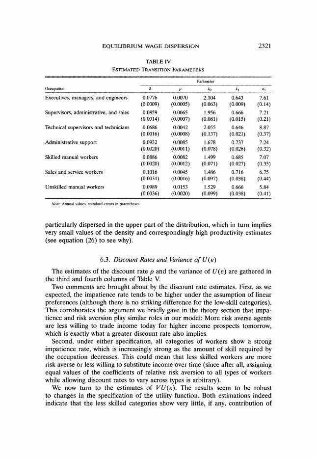
EQUILIBRIUM WAGE DISPERSION 2321
TABLE IV
ESTIMATED TRANSITION PARAMETERS
Parameter
Occupation , Ao Al K1
Executives, managers, and engineers 0.0776 0.0070 2.104 0.643 7.61 (0.0009) (0.0005) (0.063) (0.009) (0.14)
Supervisors, administrative, and sales 0.0859 0.0065 1.956 0.666 7.21 (0.0014) (0.0007) (0.081) (0.015) (0.21)
Technical supervisors and technicians 0.0686 0.0042 2.055 0.646 8.87 (0.0016) (0.0008) (0.137) (0.021) (0.37)
Administrative support 0.0932 0.0085 1.678 0.737 7.24 (0.0020) (0.0011) (0.078) (0.026) (0.32)
Skilled manual workers 0.0886 0.0082 1.499 0.685 7.07 (0.0020) (0.0012) (0.071) (0.027) (0.35)
Sales and service workers 0.1016 0.0045 1.486 0.716 6.75 (0.0031) (0.0016) (0.097) (0.038) (0.44)
Unskilled manual workers 0.0989 0.0153 1.529 0.666 5.84 (0.0036) (0.0020) (0.099) (0.038) (0.41)
Note: Annual values, standard errors in parentheses.
particularly dispersed in the upper part of the distribution, which in turn implies very small values of the density and correspondingly high productivity estimates (see equation (26) to see why).
6.3. Discount Rates and Variance of U(e)
The estimates of the discount rate p and the variance of U(e) are gathered in the third and fourth columns of Table V
Two comments are brought about by the discount rate estimates. First, as we expected, the impatience rate tends to be higher under the assumption of linear preferences (although there is no striking difference for the low-skill categories). This corroborates the argument we briefly gave in the theory section that impa- tience and risk aversion play similar roles in our model: More risk averse agents are less willing to trade income today for higher income prospects tomorrow, which is exactly what a greater discount rate also implies.
Second, under either specification, all categories of workers show a strong impatience rate, which is increasingly strong as the amount of skill required by the occupation decreases. This could mean that less skilled workers are more risk averse or less willing to substitute income over time (since after all, assigning equal values of the coefficients of relative risk aversion to all types of workers while allowing discount rates to vary across types is arbitrary).
We now turn to the estimates of VU(e). The results seem to be robust to changes in the specification of the utility function. Both estimations indeed indicate that the less skilled categories show very little, if any, contribution of

2322 F. POSTEL-VINAY AND J.-M. ROBIN
8.49386
7221766
mea
U(w)
per
Orm
mea
U(wM
per
firm
m
3qw)
per
1inn
Executives,
managers &
engineers
Supervisors,
admirstralive
and
sales
Technical
supevisors
and
tochnicans
6.09639-
6934-
6.41017 -
3.54211
43904
3.55102
4.436b6
3.4124
mnean
U(w)
per
firm
man
ULw)
per
minn
man
U(w)
per
firm
Administrative
support
Skilled
manual
workers
Sales
and
service
workers
30017 -
Solid: In p
Dashed:
45?
line
Vertical
bars at
the
10th,
25th,
50th,
-
75th
and
90th
percentiles of
Z(y).
3.46
4
19052
mean
L(AW)
firm
Unskilled
manual
workers
FIGURE
1.-Log
marginal
productivity
and
average
log-wages
(case
U(w)
ln
w).

EQUILIBRIUM WAGE DISPERSION 2323
TABLE V
ESTIMATION OF THE REMAINING PARAMETERS
Occupation Case U(b) U(Pmin) p V[U(C)]
Executives, managers, and engineers U(w) = In w 4.62 4.74 0.128 0.051 (12% annual) (0.0029)
U(w) = w 97.1 112.9 0.353 0.100 (30% annual) (0.0037)
Supervisors, administrative, and sales U(w) = In w 3.99 4.21 0.320 0.019 (27% annual) (0.0016)
U(w) = w 53.6 67.2 0.471 0.046 (38% annual) (0.0022)
Technical supervisors and technicians U(w) = In w 4.07 4.22 0.240 0.006 (21% annual) (0.0010)
U(w) = w 56.8 66.5 0.361 0.015 (30% annual) (0.0013)
Administrative support U(w) = ln w 3.69 3.84 0.678 0.007 (49% annual) (0.0014)
U(w) = w 40.0 46.5 0.678 0.012 (49% annual) (0.0014)
Skilled manual workers U(w) = ln w 3.76 3.93 0.475 -0.006 (38% annual) (0.0011)
U(w) = w 43.3 50.3 0.443 -0.001 (36% annual) (0.0013)
Sales and service workers U(w) = ln w 3.55 3.61 0.653 0.003 (48% annual) (0.0011)
U(w) = w 34.0 36.5 0.580 0.004 (44% annual) (0.0013)
Unskilled manual workers U(w) = ln w 3.54 3.63 0.834 -0.004 (57% annual) (0.0017)
U(w) = w 33.9 37.1 0.796 -0.006 (55% annual) (0.0017)
personal ability to the total variance of workers' utilities. There is little more one can say on those results, since comparing the levels of VJ and V lns makes no sense. We shall return to this point in the next section.
In any case, those large values of p, together with the fact that discount rates are usually said to be poorly identified, requires some discussion about the quality of our estimates. If we plot the GMM criterion (RMSE) used to estimate p and VU(s) for all values of p between 0.05 and 2.0, we see that the RMSE is a smooth U-shaped function of p with a clear minimum.30 Except for executives and managers in the log-utility case, values of p near to 5 or 10% per annum are clearly rejected (with an RMSE over a hundred times larger than its minimal value). Moreover, except for executives and managers, the estimated VU(s) is
30 These figures are not reproduced here to save space but they are available in the working paper, which one can find on our web pages.
2324 F. POSTEL-VINAY AND J.-M. ROBIN
always zero around p = 0.05 or 0.1. Under this restriction, the model without any individual heterogeneity would thus already generate more wage variance than is observed. Lastly, the largest estimates of the variance of person effects VU(S) are always obtained for a value of p that is above the RMSE minimizer, and the estimated VU(s) that is reported in Table V is generally close to the maximal value obtained for any p.
6.4. Within-firm Log-wage Variance
Figure 2 displays the empirical and predicted within-firm log-wage vari- ances against the corresponding within-firm mean log wages (observed (1/#Ij) ,ij [U(wi) _ yj]2 and predicted V(ln wIp = pj) against empirical yj for all firm indices j). The scattered circles correspond to the data,31 the solid line to the logarithmic-utility assumption, and the dashed line to the linear-utility case.
It is first plainly clear that the data are heteroskedastic and that the conditional log wage variance appears to be an increasing function of mean log wages. This is per se a very interesting result. It is also clear under either specification of the utility function that the model definitely picks up the correct overall correlation and the correct magnitude.
That the within-firm log-wage variance shows an increasing trend against within-firm mean log wage for all categories of labor is not an unexpected result. One indeed typically expects the distribution of wages in more productive firms (or, equivalently, in firms with large mean wages) to be more dispersed than the distribution of wages in less productive firms both because they offer lower wages to unemployed workers, due to increased monopsony power, and because they can poach the employees of the less productive firms by offering them higher income prospects. That the magnitudes are also correct is a remarkable result if one remembers how few free parameters were estimated to fit within-firm vari- ances (p and VU(?)), all other parameters being estimated so as to provide a perfect fit to within-firm mean utilities.
Nonetheless, the predicted conditional variance shows undulations that do not exist in the data and tends to overshoot its target for high p's (especially for the last four worker categories). The comparison of U(s) = s to U(s) = ln s is also interesting as it seems to indicate that the risk-neutrality assumption generates a within-firm log-wage variance that provides a (slightly) better fit for large values of within-firm mean log wage.
We end this section by a formal comparison of the ability of the model to reproduce the within-firm data on means and variances of log earnings. Table VI displays the ratios of the weighted sums of squares of predicted to actual data for the within-firm mean log earnings and within-firm log-earnings variances under both specifications of the utility functions. They correspond to the R2 of the
31 To be precise, we plotted only 500 points, each point corresponding to a different evaluation of the conditional log-wage variance given mean log wage y, for 500 equidistant values of mean log wages in the interval [Ymin ymx]. Nadaraya-Watson kernel estimators of conditional means are used to smooth the empirical conditional variance using the formula: VX = EX2 - (EX)2.
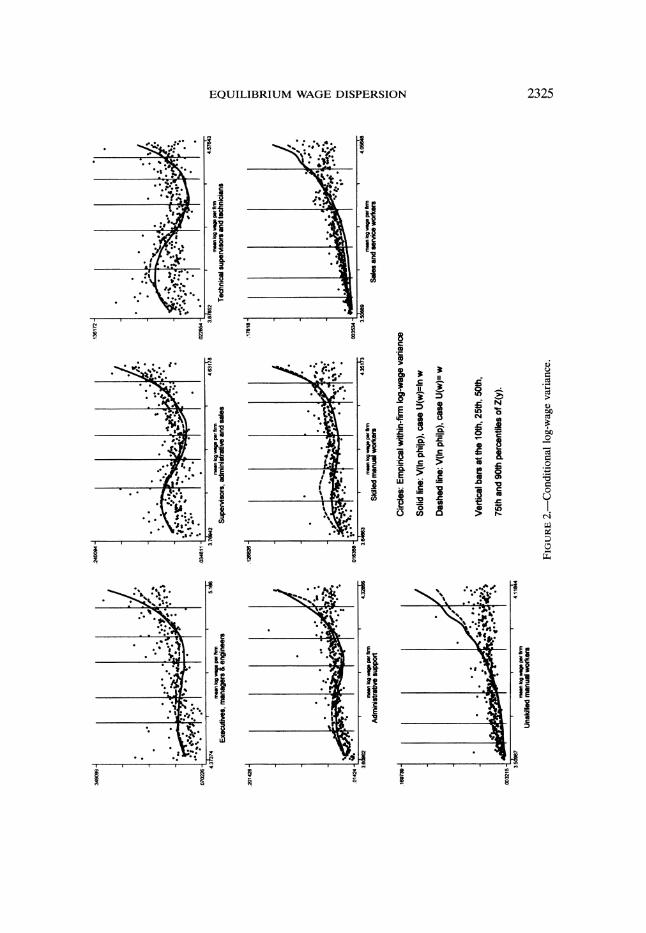
EQUILIBRIUM WAGE DISPERSION 2325
.349099 -
240094
136172 -
rWn
bg
p*, n ,, F pe, n , lW WW PC 11frV..
.
.070226
43481 1
.=854 8
k3A874
'
'.
3.76342
4.6358
3.8h52
4.57643
man
tog
wp
per
fim
meann I
wOe
per
fm
manlgwae P.
frlm
ExecAuives,
managr
&
engineers
Supervisr,
adnnstrsve
and
sales
Technical
supervi
n
tochnons
32D1426
126026
-.17818-
%~~~~~~~~~~~~~~~~~~~
%~~~~~~~~~~~~~~~~~~~~~~~~~~~~~~~~~~~~~~~~~~~~~
.
Aww~~~~~~~~~~~~~~~~~~~~~~~~~~~~~~~~~~~9
.014241-5AM6358
O.353
_
3______________________ -
430
3.64883
435153
3
4.01118
mwn b
wv
per
flnmnn
e
erfr
Adnirdstraive
support
komanual
worke
Circles:
Empirical
wihin-firm
log-wage
variance
Solid
line:
V(ln
phitp),
case
U(w)=1n w
00
~~~~Dashed
line:
V(ln
philp),
case
U(w)= w
*
* *
*Lj***E
~~~~~~~Vertical
bamsat
thelIOth,
25th,
50th,
75th
and 90t
percentiles of
Z(y).
Unskilled
manual
workers
FIGURE
2.-Conditional
log-wage
variance.

2326 F. POSTEL-VINAY AND J.-M. ROBIN
TABLE VI
GOODNESS OF FIT STATISTICS FOR FIRM DATA
Occupation Case Mean log wagea Log-wage variancea
Executives, managers, and engineers U(w) = In w 0.9997 1.226 U(w) = w 1.0178 1.133
Supervisors, administrative, and sales U(w) = In w 1.0004 1.213 U(w) = w 1.0076 1.159
Technical supervisors and technicians U(w) = In w 1.0001 1.364 U(w) = w 1.0024 1.185
Administrative support U(w) = In w 0.9994 1.306 U(w) = w 1.0018 1.238
Skilled manual workers U(w) = In w 1.0005 1.613 U(w) = w 0.9986 1.913
Sales and service workers U(w) = In w 0.9993 2.214 U(w) = w 1.0000 1.597
Unskilled manual workers U(w) = In w 0.9992 3.824 U(w) = w 0.9985 2.703
aR2 of the weighted regression of actual on predicted (no constant, regression coefficient = 1).
weighted regression of actual on predicted variables with no intercept when the coefficient of the predicted variable is constrained to one. It is clear that the model reproduces very accurately the within-firm mean log wages even for the linear-utility case, although the productivity estimates were chosen so as to pro- vide the best fit to within-firm mean wages instead of mean log wages, indicating that Identifying Assumption 2 is well accepted by the data for both specifications of the utility function. The prediction of mean log wages is thus not going to be of much help as a criterion to choose between different risk aversion coefficients. The results on variances are more informative. First the R2 is always greater than 1, indicating the model's tendency to overpredict the within-firm variance of log earnings in the upper part of the distribution of within-firm mean log wages. This is particularly true for the less skilled categories. Second, confirming the previous visual impression, the linear utility seems to produce less overshooting than the logarithmic utility in most cases.
6.5. Individual Log-wage Variance Decomposition
We now analyze the results of the log-wage variance decomposition described in Section 3.5. Simulating a cross-section of values of 0(1, q, p), as indicated in Section B.3.1 of the Appendix, allows us to compute the last two terms in the right-hand side of the decomposition formula (12). We obtain a "global" estimate of V ln ? by taking the difference to V ln w.32
32 Note that, in the log-utility case, another estimator of V In e is available from the conditional variance regression (see the second paragraph in Appendix B.2). The two estimators give close results (see Tables V and VII).
EQUILIBRIUM WAGE DISPERSION 2327
The log-wage variance decomposition is reported in Table VII. First, we can note that both specifications of the preferences result in similar shares of each effect in the explanation of total log-wage variance. At the very least, the quali- tative picture is the same under either assumption. The model thus successfully passes this robustness test. Second, and more importantly, we obtain a remark- able result: individual ability differences explain about 40% of the log-wage variance for executives, managers and engineers, 20% for workers with lower executive functions, 10% for technicians and technical supervisors and the admin- istrative support staff, and virtually nothing for the other categories. It therefore seems that the more sophisticated the occupation is, the more difficult it is to predict the efficiency of a worker given his observable attributes. To put it dif- ferently, the more skill-intensive an occupation is, the more heterogeneous is the category of workers who can apply to it. At the bottom of the skill hierarchy, manual workers and employees are rather homogeneous as far as productive efficiency is concerned. In all cases, a significantly more important share of the variance (45 to 60%) is due to differences in individual histories, which are cap- tured by the friction effect term in our decomposition formula (12).
As a matter of comparing our results to those of previous contributions, again we should cite AKM and Abowd and Kramarz (2000), who use the same data as we do, but on a different time span, and find over the whole sample, controlling for observed skill characteristics, that the person effect accounts for more or less 50% of total log-wage variance. Even though we ran separate estimations for each skill category, our results make it clear that the average weight of the person effect over the whole sample is by far less than a half.
The credibility of these results rests on Identifying Assumption 3 that mean earnings utilities correctly sort the firms by unobserved productivities. Remem- ber that because many of these firms have small sizes, mean earnings utilities are thus subject to statistical errors, for example due to fluctuations around the equilibrium value that the model predicts.33 It may thus be that many firms have erroneously been assigned equal productivity values. Now, clearly, any realloca- tion of firms into different productivity clusters will end up reducing the ability of the productivity indicator to explain the dispersion of individual earnings util- ities and, hence, increasing the share of individual heterogeneity. Our current estimates are therefore to be thought of as lower bounds for the contribution of person effects to the log-wage variance.
In order to analyze the sensitivity of our results with respect to sampling errors, we adopt a Bayesian perspective and consider the asymptotic approximation:
(14) Yj < NE[U(w)lp=p] V[U(w)p = p1j]
which holds for large firm sizes, as a prior for mean utilities E[U(w)lp = pj]. In other words, we start from the belief that the true mean earnings utility
33 Here we discuss estimation errors in the context of a well specified model. Any source of model misspecification, like human capital accumulation generating changes in the workers' abilities, is of course another potential source of estimation error, which requires a proper model to be analyzed.
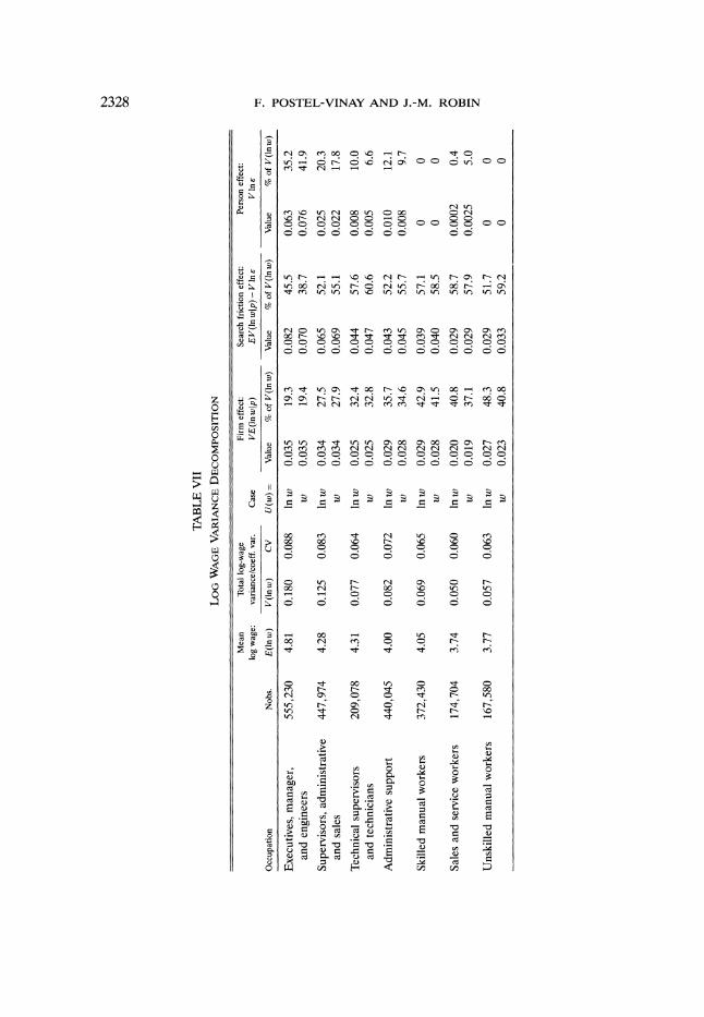
2328 F. POSTEL-VINAY AND J.-M. ROBIN
TABLE
VII
LOG
WAGE
VARIANCE
DECOMPOSITION
Mean
Total
log-wage
Firm
effect:
Search
friction
effect:
Person
effect:
log
wage:
variance/coeff.
var.
Case
VE(ln
wlp)
EV(ln
wlp) - V In E
VInE
Occupation
Nobs.
E(ln w)
V(ln w)
CV
U(w) =
Value
% of
V(ln w)
Value
% of
V(ln w)
Value
% of
V(ln w)
Executives,
manager,
555,230
4.81
0.180
0.088
In w
0.035
19.3
0.082
45.5
0.063
35.2
and
engineers
w
0.035
19.4
0.070
38.7
0.076
41.9
Supervisors,
administrative
447,974
4.28
0.125
0.083
Inw
0.034
27.5
0.065
52.1
0.025
20.3
and
sales
w
0.034
27.9
0.069
55.1
0.022
17.8
Technical
supervisors
209,078
4.31
0.077
0.064
In w
0.025
32.4
0.044
57.6
0.008
10.0
and
technicians
w
0.025
32.8
0.047
60.6
0.005
6.6
Administrative
support
440,045
4.00
0.082
0.072
In w
0.029
35.7
0.043
52.2
0.010
12.1
w
0.028
34.6
0.045
55.7
0.008
9.7
Skilled
manual
workers
372,430
4.05
0.069
0.065
Inw
0.029
42.9
0.039
57.1
0
0
w
0.028
41.5
0.040
58.5
0
0
Sales
and
service
workers
174,704
3.74
0.050
0.060
lnw
0.020
40.8
0.029
58.7
0.0002
0.4
w
0.019
37.1
0.029
57.9
0.0025
5.0
Unskilled
manual
workers
167,580
3.77
0.057
0.063
lnw
0.027
48.3
0.029
51.7
0
0
w
0.023
40.8
0.033
59.2
0
0

EQUILIBRIUM WAGE DISPERSION 2329
of employees of firm j is yj plus an error uj that has a normal distribution with mean 0 and variance the empirical within-firm variance divided by firm size: (1/(#Ij)2) Eij[U(wi)yj]2. In order to evaluate the consequences in terms of the decomposition of log-wage variances, we simulate alternative values YJ = yJ + u8 by adding a simulated error term Us drawn from the relevant normal distribution to the observed y1 for all establishments of the sample, and reesti- mate the model with the new mean utility values as for the actual data. Note that firms that were originally assigned close productivities because they had close mean utility values in the original sample can now end up at very distant points of the distribution of p's, particularly if their small sizes imply a relatively large error variance. We repeat the experiment 500 times for each occupation and each specification of the preferences. Table VIII below reproduces certain quan- tiles of the posterior distributions of the shares of each effect (person, firm, and friction) in the explanation of total log-wage variance, as well as those of the estimated annual discount factor (1 - e-P).
What Table VIII shows is that none of those estimates are dramatically affected by sampling errors. All reported distributions are very concentrated (albeit with quite long tails). Looking at the medians and comparing them to the point esti- mates of Table VII, we see that, as expected, "shuffling" the establishments as we do in this sensitivity check diminishes the explanatory power of the firm effect and reinforces that of the person effect. But the general order of magnitude of the discrepancy is only a few percentage points. Only in the case of sales and service workers with linear preferences does the estimated share of the person effect seem to really be on the low side in terms of the distribution sketched in Table VIII (the estimated value using the original sample is 5% , while the 5th and 10th percentiles of the posterior distribution of the estimator taking account of sampling errors are 0 and 9% respectively). This may be due in part to the rel- atively high density of small establishments in this occupational category. Finally, concerning the annual discount factor, a comparison with the values obtained in Table V reveals no general pattern in the discrepancies, and suggests that the estimate of p is also reasonably insensitive to sampling errors.
6.6. Cross-sectional Earnings Distributions
All the parameters of the model being now estimated, and the validity of Iden- tifying Assumptions 2 and 3 assessed, we can simulate the model and compare the actual distributions of earnings to the predicted ones. Figure 3 provides, for each of the seven professions we consider, the graphs of the quantile functions for the distribution of individual log wages and the distribution of ln 4(1, q, p) when (p, q) is distributed as explained in Section 3.4.34 The latter distribution is the distribution predicted by the model when there is no dispersion of abilities.
34 The figure shows the results for the log-linear utility case as the linear utility case shows similar patterns. Appendix B.3.1 explains the simulation technique that we use to compute these quantile functions.

2330 F. POSTEL-VINAY AND J.-M. ROBIN
TABLE
VIII
POSTERIOR
DISTRIBUTIONS
OF
SOME
PARAMETERS Quantiles
Case
U(w)=lnw
Case
U(w)=Inw
Occupation
Parameter
(%)
5%
10%
50%
90%
95%
5%
10%
50%
90%
95%
Executives,
Annual
discount
8.8
9.5
11.5
13.5
14.6
21.1
29.7
35.1
40.9
43.7
managers,
Share of
firm
effect
17.5
17.6
17.8
18.0
18.1
17.7
17.8
18.0
18.3
18.8
and
engineers
Share of
frictions
39.1
40.0
42.6
46.0
46.9
28.1
29.0
31.4
34.6
43.9
Share of
person
effect
35.4
36.1
39.6
42.2
43.2
37.4
47.4
50.7
53.0
53.8
Supervisors,
Annual
discount
11.3
17.4
20.3
24.3
69.7
14.1
31.1
38.7
43.6
56.9
administrative,
Share of
firm
effect
25.2
25.2
25.5
25.9
26.4
24.3
24.6
24.9
25.3
26.2
and
sales
Share of
frictions
46.1
50.2
53.0
55.5
64.1
34.0
44.7
48.8
52.0
57.8
Share of
person
effect
4.8
18.3
21.4
24.2
27.6
2.6
22.5
26.2
29.5
37.9
Technical
Annual
discount
7.7
13.2
16.1
19.4
20.6
11.6
24.2
29.4
33.2
50.8
supervisors
Share of
firm
effect
30.7
30.8
31.3
31.8
32.1
30.8
31.1
31.6
32.7
35.4
and
technicians
Share of
frictions
51.3
55.7
59.1
62.8
67.2
39.9
54.4
58.3
62.5
65.1
Share of
person
effect
0
3.6
9.6
12.7
14.1
0
1.2
10.1
13.6
15.6
Administrative
Annual
discount
16.8
28.8
35.1
41.3
43.7
14.1
29.5
49.2
59.8
99.2
support
Share of
firm
effect
33.7
33.8
34.1
34.5
34.6
28.0
32.3
32.8
33.7
34.6
Share of
frictions
52.0
52.8
55.7
59.6
65.3
37.0
47.4
52.6
63.8
65.7
Share of
person
effect
0
6.0
10.2
13.0
13.8
0
0
14.4
19.6
34.3
Skilled
Annual
discount
24.7
25.3
27.1
29.1
29.1
19.2
26.5
30.6
33.9
39.5
manual
Share of
firm
effect
40.3
40.4
40.7
41.1
41.2
38.7
38.8
39.1
39.8
41.7
workers
Share of
frictions
58.8
58.9
59.3
59.6
59.7
56.6
59.9
60.9
61.2
61.3
Share of
person
effect
0
0
0
0
0
0
0
0
0
0
Sales
and
Annual
discount
27.3
29.9
33.0
34.6
36.4
16.5
41.6
48.0
50.9
50.9
service
Share of
firm
effect
38.2
38.4
38.9
39.6
39.9
33.0
34.1
35.0
35.7
35.9
workers
Share of
frictions
60.0
60.3
61.1
61.6
61.8
50.5
51.0
52.6
55.8
67.0
Share of
person
effect
0
0
0
0
0.3
0
9.0
12.3
14.0
14.7
Unskilled
Annual
discount
21.9
37.5
39.4
41.5
42.6
17.4
46.2
48.9
51.7
51.7
manual
Share of
firm
effect
46.1
46.3
47.0
47.6
47.7
37.6
38.7
39.5
40.2
40.3
workers
Share of
frictions
52.3
52.4
53.0
53.7
53.9
59.4
59.6
60.4
61.2
62.4
Share of
person
effect
0
0
0
0
0
0
0
0
0.8
1.3
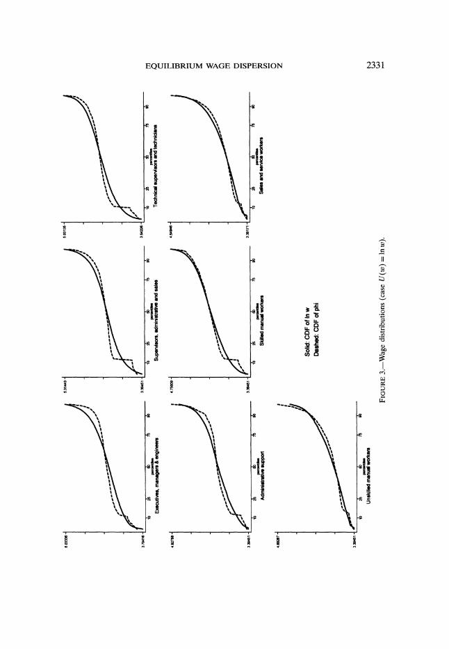
EQUILIBRIUM WAGE DISPERSION 2331
6.03336
5.31443
5.03135
370
10
35
do
is
do
3.95
10
gs o
/s
d
10
55422'
d
per=-t-
pesosh-
peroerhs
Executives,
managrs &
engineers
Supervisors,
adrrinistrfive
and
sales
Technical
supervsors
and
technicians
492786 -
475006
454946
3.39451 -
3.39451
3.39171
3
10
25
do
A~d
0
i
do
A5
do1
5
oi
d
perouts
Psross
PWaess
Adrninistrative
support
Skiled
manual
workers
Sales
and
service
workers
4.667 -
Solid:
CDF of In w
Dashed:
CDF of phi
3.39451-
10
25
do
'5
90
Per0
Unskilld
manual
workers
FIGURE
3.-Wage
distributions
(case
U(w) = In
w).

2332 F. POSTEL-VINAY AND J.-M. ROBIN
First, we observe a discontinuity in the quantile function for In 0(1, q, p) that is entirely due to the gap between b and Pmin. It is plainly clear that U(Pmin) - U(b) is far too large for the distribution of wages offered to former unemployed to be jointed with the distribution of wages obtained from on-the-job search. The data seem to require heterogeneity in b as well as heterogeneity in E to mix the lower part of the distribution of predicted wages and provide a better fit. We leave this extension to further work.35
Second, one sees why we estimate no ability dispersion for low skilled workers. The model with no worker heterogeneity works quite well to explain the disper- sion of log earnings in this case. For skilled manual workers, the fit is good in the upper part of the distribution but bad in the lower part because of the wide wedge between U(Pmin) and U(b).
The distribution of log wages is equal to the convolution of the distribution of ln 0(1, q, p) with the distribution of ln E, i.e. H. Figure 4 plots the deconvolution results using the method described in Appendix B.3 for the first four categories.36 The estimates for the linear and logarithmic cases are superimposed on the same graphics to emphasize the differences. It turns out that there are strikingly few dif- ferences. The choice of the utility function therefore has a very limited impact on the estimated distribution of unobserved worker abilities. Moreover, as it should be given the preceding estimates of V ln 8, the distribution for the first group of workers is flatter than that for the second group, which is itself flatter than the last two. The right tail of the distribution of ln E is also thicker for the first group.
For the first four categories of more skilled workers, the actual distribution of wages dominates the predicted one (with no worker heterogeneity) in the upper part of the distribution. This demonstrates the necessity of allowing for hetero- geneous abilities, which we now do. As is also explained in Appendix B.3, the deconvolution method can also deliver the cdf's of ln E, from which we can get random draws of worker abilities and thus simulate a complete cross-section of wages (in fact, all we have to do at this point is add a cross section of ln E's randomly selected from H to the cross section of ln 0(1, q, p)'s already simu- lated). The predicted cross-worker log-wage densities are plotted together with the observed ones on Figure 5 (densities are estimated using a normal kernel). We see that the fit is improved, except at the left end of the wage distribution. This again points to the need of some heterogeneity in the workers' "at-home" productivity parameters, b.
Note that standard goodness of fit tests like the chi-squared or Kolmogorov- Smirnov tests always reject the null that the model is correctly specified. This was to be expected given the large sample sizes. Table IX displays the chi-squared and Kolmogorov-Smirnov statistics divided by sample sizes for each estimated log-earnings distribution.37 The corresponding p-values are not reported as they
35 Heterogeneity in b is present in the theoretical model that we constructed in a previous paper (Postel-Vinay and Robin (1999)).
36 Our attempts at retrieving a nondegenerate distribution of ln ? for the remaining three categories failed, as expected given that their estimated variance of ln ? was 0.
37 How we exactly compute the chi-square and K-S statistics is explained in a note to Table IX.
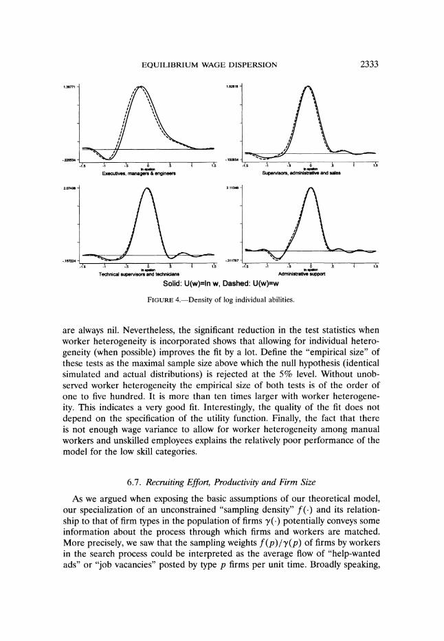
EQUILIBRIUM WAGE DISPERSION 2333
1.39771 1.82818 ''n' '""'~~~~/
-22&534 A .150154-
-tl.5 -1 -'5 ^ .i 4 1.5 -15 1 15 .5 t5 In epdbn In spal
Execufive, managers & engineers Supervisors, adminisbutive and sales
2.0749e - 2.113446-
-t'.5 ~~~ ~ -t15 * 5 t1'.5 -t -5 6 .A I ' In dbn In ep*lb
Technical supervsors and technicians Adminishive support
Solid: U(w)=ln w, Dashed: U(w)=w
FIGURE 4.-Density of log individual abilities.
are always nil. Nevertheless, the significant reduction in the test statistics when worker heterogeneity is incorporated shows that allowing for individual hetero-
geneity (when possible) improves the fit by a lot. Define the "empirical size" of these tests as the maximal sample size above which the null hypothesis (identical simulated and actual distributions) is rejected at the 5%o level. Without unob- served worker heterogeneity the empirical size of both tests is of the order of one to five hundred. It is more than ten times larger with worker heterogene- ity. This indicates a very good fit. Interestingly, the quality of the fit does not
depend on the specification of the utility function. Finally, the fact that there is not enough wage variance to allow for worker heterogeneity among manual workers and unskilled employees explains the relatively poor performance of the model for the low skill categories.
6.7. Recruiting Effort, Productivity and Firm Size
As we argued when exposing the basic assumptions of our theoretical model, our specialization of an unconstrained "sampling density" ff () and its relation- ship to that of firm types in the population of firms Py( ) potentially conveys some information about the process through which firms and workers are matched. More precisely, we saw that the sampling weights f (p) I y(p) of firms by workers in the search process could be interpreted as the average flow of "help-wanted ads" or "job vacancies" posted by type p firms per unit time. Broadly speaking,
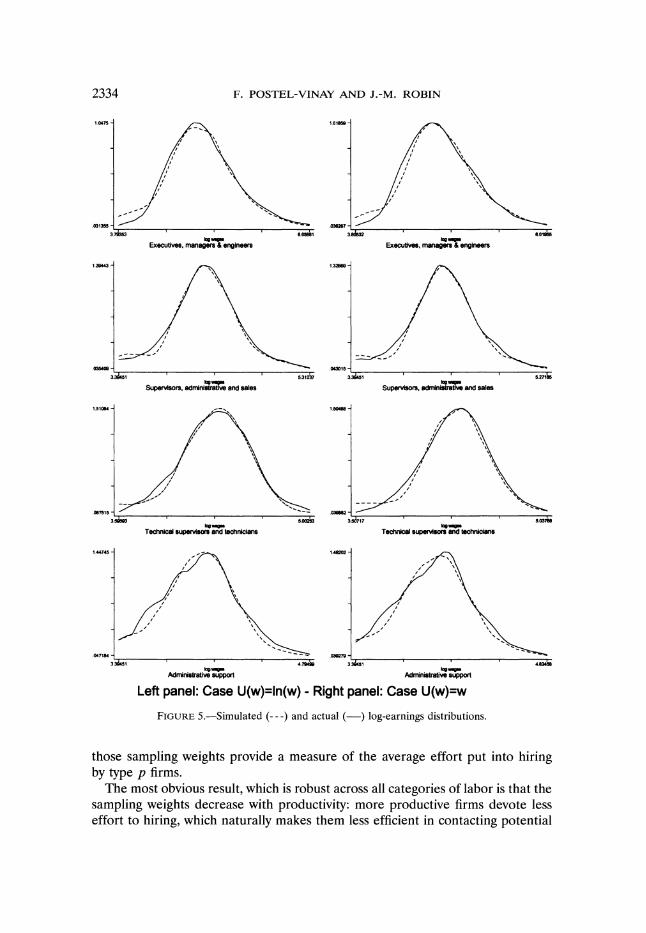
2334 F. POSTEL-VINAY AND J.-M. ROBIN
1.0475 - i.01M -~~~~~~~~~~~~~~~~~~~~~~~~~~~~~~~~~~~~~~~6.16
Execuffves, managers & engineers Executives, manag & engineers
1.269431 g a q 1.3205
3.3461 5.31727 3.3;401 5.271kS
Supervisors, adinistrZave and sales Supervisors, administrative and sales
1.510B4 - 1.504
.09751:d3 -o .032j= 5-
Technical supervisors and technicians Technica superviso and technicians
1.44745 1.46252
.047184 *039279
3.36451~~~~~~~~~~~~~~~~~~~~~~~~~~~~~~~~~~~~~~~~~~~.36 Adrrinistative support Adninistrative suppor
Left panel: Case U(w)=ln(w) - Right panel: Case U(w)=w
FIGURE 5.-Simulated (--- ) and actual (-) log-earnings distributions.
those sampling weights provide a measure of the average effort put into hiring by type p firms.
The most obvious result, which is robust across all categories of labor is that the sampling weights decrease with productivity: more productive firms devote less effort to hiring, which naturally makes them less efficient in contacting potential
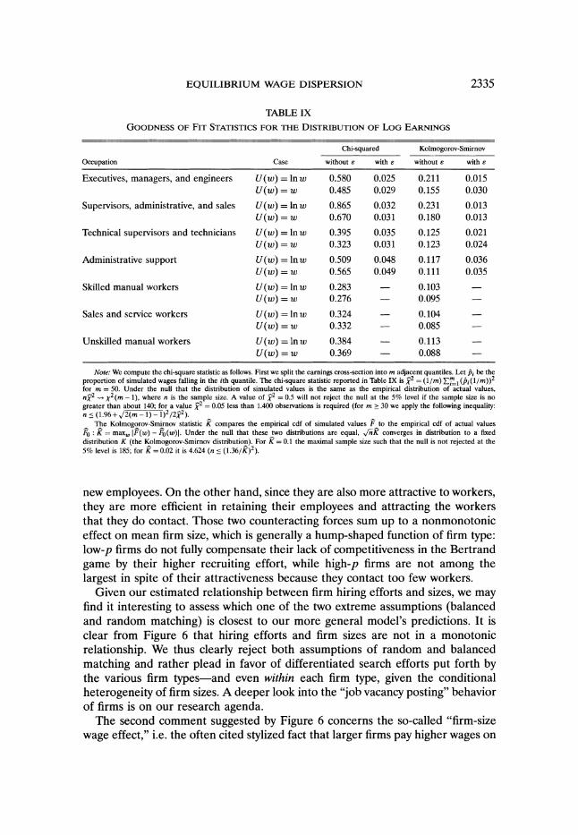
EQUILIBRIUM WAGE DISPERSION 2335
TABLE IX
GOODNESS OF FIT STATISTICS FOR THE DISTRIBUTION OF LOG EARNINGS
Chi-squared Kolmogorov-Smirnov
Occupation Case without E with E without E with E
Executives, managers, and engineers U(w) = In w 0.580 0.025 0.211 0.015 U(w) = w 0.485 0.029 0.155 0.030
Supervisors, administrative, and sales U(w) = In w 0.865 0.032 0.231 0.013 U(w) = w 0.670 0.031 0.180 0.013
Technical supervisors and technicians U(w) = In w 0.395 0.035 0.125 0.021 U(w) = w 0.323 0.031 0.123 0.024
Administrative support U(w) = nw 0.509 0.048 0.117 0.036 U(w) = w 0.565 0.049 0.111 0.035
Skilled manual workers U(w) = In w 0.283 - 0.103 U(w) = w 0.276 0.095
Sales and service workers U(w) = ln w 0.324 - 0.104 U(w) = w 0.332 - 0.085
Unskilled manual workers U(w) = nw 0.384 - 0.113 U(w) = w 0.369 0.088
Note: We compute the chi-square statistic as follows. First we split the earnings cross-section into m adjacent quantiles. Let Pi be the proportion of simulated wages falling in the ith quantile. The chi-square statistic reported in Table IX is x2 = (1/m) Em (fi(1/m))2 for m = 50. Under the null that the distribution of simulated values is the same as the empirical distribution of actual values, nX2 _+ 2(m - 1), where n is the sample size. A value of x2 = 0.5 will not reject the null at the 5% level if the sample size is no greater than about 140; for a value x2 = 0.05 less than 1.400 observations is required (for m > 30 we apply the following inequality: n < (1.96+,?/2(m-1)- /2j2).
The Kolmogorov-Smirnov statistic K compares the empirical cdf of simulated values F to the empirical cdf of actual values Fo: K = max. IF(w) - Fo(w)1. Under the null that these two distributions are equal, l/hk converges in distribution to a fixed distribution K (the Kolmogorov-Smirnov distribution). For K = 0.1 the maximal sample size such that the null is not rejected at the 5% level is 185; for k = 0.02 it is 4.624 (n < (1.36/k)2).
new employees. On the other hand, since they are also more attractive to workers, they are more efficient in retaining their employees and attracting the workers that they do contact. Those two counteracting forces sum up to a nonmonotonic effect on mean firm size, which is generally a hump-shaped function of firm type: low-p firms do not fully compensate their lack of competitiveness in the Bertrand game by their higher recruiting effort, while high-p firms are not among the largest in spite of their attractiveness because they contact too few workers.
Given our estimated relationship between firm hiring efforts and sizes, we may find it interesting to assess which one of the two extreme assumptions (balanced and random matching) is closest to our more general model's predictions. It is clear from Figure 6 that hiring efforts and firm sizes are not in a monotonic relationship. We thus clearly reject both assumptions of random and balanced matching and rather plead in favor of differentiated search efforts put forth by the various firm types-and even within each firm type, given the conditional heterogeneity of firm sizes. A deeper look into the "job vacancy posting" behavior of firms is on our research agenda.
The second comment suggested by Figure 6 concerns the so-called "firm-size wage effect," i.e. the often cited stylized fact that larger firms pay higher wages on

2336 F. POSTEL-VINAY AND J.-M. ROBIN
95441 1
3.82055
.972501
3.33833
899367
-3.6943
-2.26756
3.39002
-1.90719
31125
-2.01148
302925
414814
601823
4.2i701
5.3042
42d805
033
5(p)
U(p)
(AP)
Execuives,
managers &
engineers
Supervisors,
administrative
and
sales
Technical
supervisors
and
technicians
,795694-
3.65266
.625473
-3.69757
~
892004-
301951
-1.96107
3.12279
-1.87388
2.59735
-1.98899
2.65258
3.0637
5.02863
3.8611
4.89791
3.6508
4.6731
5(p)
5(p)
5(p)
Administrative
support
Skilled
manual
workers
Sales
and
seMce
workers
1.15875
3.25354
Z
\ \
/
E
Solid:
ln[l(p)/gamma(p)]
Dashed:
ln[f(p)/gamma(p)J
-1.786081 -
. S 2608977
3.6d71
4.723&4
U(p)
Unskilled
manual
workers
FIGURE
6.-Recruiting
effort,
productivity,
and
size.

EQUILIBRIUM WAGE DISPERSION 2337
average. Given that mpl's and mean log wages are in an increasing relationship with each other in our model, one should thus expect the relationship of p to firm sizes to be upward sloping. What Figure 6 seems to suggest is that this is only true at the lower levels of productivity and/or average wages. This result only apparently contradicts the "firm-size wage effect." Going back to the raw data and looking at the empirical relationship between firm sizes and average wages, it is easy to check that, even though the coefficient of a linear regression of (log) firm sizes against mean log wages is admittedly positive (albeit relatively small), a regression of (log) firm sizes against a second-order polynomial of mean log wages precisely predicts this hump shape.
7. DYNAMIC SIMULATIONS
The most severe specification test of which we could conceive is to look at how good (or bad) the model is at predicting wage mobility along the line of Tables II and III on which we have already commented. Tables X and XI display the results of a dynamic simulation of 10,000 trajectories for each professional category. The main discrepancy between real and simulated data is that the model does not do well (to say the least) in predicting downward wage mobility. We produce rather good upward wage mobility predictions for workers changing employers (the last two columns of Tables II and X are quite close). Yet, the simulations are clearly not as good for those workers holding the same job over the one year simulation period since we predict too few downward and upward wage changes. This is true in particular for the low-skilled categories.
TABLE X
DYNAMIC SIMULATION VARIATION IN REAL WAGE AFTER
FIRST RECORDED JOB-TO-JOB MOBILITY
Median % obs. such that A log wage <
Occupation Case Alog wage (%) -0.10 -0.05 0 0.05 0.10
Executives, managers, and engineers U(w) = in w 3.1 13.0 22.9 38.8 55.1 65.4 U(w) = w 3.7 7.9 17.3 34.9 54.0 65.1
Supervisors, administrative, and sales U(w) = In w 3.3 2.7 12.4 35.0 55.8 66.7 U(w) = w 2.6 3.3 11.2 34.2 57.9 69.7
Technical supervisors and technicians U(w) = In w 2.8 4.2 10.0 32.2 57.8 71.8 U(w) = w 3.9 2.9 9.0 34.2 54.8 69.3
Administrative support U(w) = nw 5.1 1.1 6.1 24.3 49.7 64.4 U(w) = w 5.3 1.0 5.2 24.0 49.2 63.8
Skilled manual workers U(w) = ln w 4.5 1.7 7.5 28.2 51.7 66.0 U(w) = w 4.4 4.3 12.4 30.6 51.7 64.7
Sales and service workers U(w) = ln w 3.0 0.2 5.5 31.0 59.1 75.3 U(w) = w 3.4 2.0 8.2 30.7 57.2 75.1
Unskilled manual workers U(w) = ln w 3.6 0.2 4.4 29.4 55.5 70.0 U(w) = w 2.7 1.0 7.3 32.4 58.6 70.0

2338 F. POSTEL-VINAY AND J.-M. ROBIN
TABLE XI
DYNAMIC SIMULATION YEARLY VARIATION IN REAL WAGE WHEN HOLDING
THE SAME JOB OVER THE YEAR
Median % obs. such that A log wage <
Occupation Case Alog wage (%) -0.10 -0.05 0 0.05 0.10
Executives, managers, and engineers U(w) = In w 0 0 0 85.8 93.9 96.6 U(w) = w 0 0 0 84.2 93.7 96.8
Supervisors, administrative, and sales U(w) = In w 0 0 0 84.7 94.8 97.3 U(w) = w 0 0 0 84.5 95.1 97.3
Technical supervisors and technicians U(w) = In w 0 0 0 87.2 95.8 97.9 U(w) = w 0 0 0 85.9 96.1 98.1
Administrative support U(w) = In w 0 0 0 84.9 94.7 97.3 U(w) = w 0 0 0 82.9 94.9 97.2
Skilled manual workers U(w) = In w 0 0 0 85.6 94.5 97.2 U(w) = w 0 0 0 83.7 94.2 96.8
Sales and service workers U(w) = ln w 0 0 0 84.0 94.9 97.5 U(w) = w 0 0 0 82.8 94.8 97.4
Unskilled manual workers U(w) = ln w 0 0 0 84.5 94.2 96.8 U(w) = w 0 0 0 82.6 94.4 97.3
A better capacity of predicting wage dynamics would have been suspect as it is unbelievable that all job mobilities with wage cuts could be explained by the option-value motive. A large part of wage mobility is likely to reflect idiosyncratic labor productivity shocks, as about 15 to 20% of earnings are bonuses that are indexed to firm performances. They can naturally (partly) be explained by moral hazard considerations but they are also likely to reflect exogenous fluctuations in market conditions or firm productivity. Another item to add to the research agenda is thus an extension of the model to allow for idiosyncratic productivity shocks, maybe along the lines of Mortensen and Pissarides (1994).
8. CONCLUDING REMARKS
The main contribution of this paper is an investigation of the properties of the distribution of wages within an equilibrium job search model with on-the-job search, using matched employer and employee data. The theoretical model features heterogeneous productivity attributes for both firms and workers, and an original wage setting mechanism that departs from the conventional alterna- tive assumptions of wage posting or wage bargaining. The model provides new results about the decomposition of log-wage variance into three components: a firm effect, a person effect, and an effect of labor market frictions. Its success at fitting the data and passing specification tests is overall satisfactory.
Now it is obvious that many important components of wage dispersion have been assumed away: Idiosyncratic productivity shocks, wage bargaining, individ- ual changes in ability and compensating differentials, let alone the fact that wage posting might be a better assumption for the wage setting mechanism at work

EQUILIBRIUM WAGE DISPERSION 2339
on low-skilled labor markets, are potential sources of wage mobility. Their omis- sion might be responsible for an overestimation of the role of search frictions in determining wage dispersion. Yet, the fact that we have been able to construct and rather easily estimate the complicated model of this paper is, we believe, by itself an important methodological achievement as it opens the way to the esti- mation of even more comprehensive equilibrium models of the labor market.
INRA, Centre Paris-Jourdan, 48, boulevard Jourdan, 75014 Padis, France, and CEPR, London, UK.; fpostel@ delta.ens.fr; http://www.inra.fr/Internet/Departments/ ESR/UR/lea/fpostel. htm/
and INRA, Centre Paris-Jourdan, 48, boulevard Jourdan, 75014 Paris France, CREST-
INSEE, Malakofft France, and CEPR, London, UK; [email protected]; http://www. infra.fr/Internet/Departements/ESR/UR/lea/robin.htm/
Manuscript received November, 2000; final revision received January, 2002.
APPENDIX A: DETAILS OF SOME THEORETIcAL RESULTS
A.1. Equilibrium Wage Determination
In this Appendix we derive the precise form of equilibrium wages 4(s, p, p'). The first step is to compute the value functions VO(.) and V(.). Since offers accrue to unemployed workers at rate AO, Vo(8) solves the following Bellman equation:
(p + / + AO)Vo(S) = U(sb) + AoEF{V(L, o(? X), X)},
where EF is the expectation operator with respect to a variable X that has distribution F. Using definition (1) to replace V(s, 4o(s, p), p) by Vo (s) in the latter equation then shows that
(15) V (S) U(sb)
We thus find that an unemployed worker's expected lifetime utility depends on his personal ability s only through the amount of output he produces when engaged in home production, sb. This naturally results from the fact that his first employer is able to appropriate the entire surplus generated by the match until the worker gets his first outside offer. The only income for which the employer originally has to compensate the worker is sb.
Now turning to employed workers, consider a type-s worker employed at a type-p firm and earning a wage w < sp. This worker is hit by outside offers from competing firms at rate A1. If the offer stems from a firm with mpl p' such that 4(s, p', p) < w, then the challenging firm is obviously less attractive to the worker than his current employer since it cannot even offer him his current wage. The worker thus rejects the offer and continues his current employment relationship at an unchanged wage rate. Now if the offer stems from a type-p' < p firm such that w < 4(S, p', p) < ?p, then the offer is iiiatched by p, in which case the challenging firm p' will not be able to attract the worker but the incumbent employer will have to grant the worker a raise-up to 4(s, p', p)-to retain him from accepting the other firm's offer. This leaves the worker with a lifetime utility of V(s, sp', p'). Finally, if the offer originates from a firm more productive than p, then the worker eventually accepts the outside offer and goes working at the type-p' firm for a wage 0(s, p, p') and a utility V(?, Sp, p).
For a given worker type-s and a given mpl p, define the threshold mpl q(s, w, p) by
4(s, q(s, w, p), p) = W,
2340 F. POSTEL-VINAY AND J.-M. ROBIN
so that k(s, p', p) < w if p' < q(&, w, p). Contacts with firms less productive than q(8, w, p) end up not causing any wage increase because the current employer (with a technology yielding productivity p) can outbid such a challenging firm by offering a wage lower than w. Since in addition layoffs and deaths still occur at respective rates 8 and ,u, we may now write the Bellman equation solved by the value function V(s, w, p):
(16) [p + 8 + ,u + A1 F(q(s, w, p))] V(8, w, p)
= U(w) + A [F(p) - F(q(s, w, p))]EF{V(8, ?X, X)Iq(s, w, p) < X < p}
+ A 1F(p)V(s, sp, p) + 8Vo(s).
Imposing w = sp in the latter relationship, we easily get
(17) V(' Sp, p) = (Sp) +5Vo(?)
Note that this expression is independent of the particular form of the unemployment value Vo(s). Plugging this back into (16), replacing the expectation term by its expression, and integrating by
parts, we finally get a definition of V(.):
(18) (p?8 +,+)V(8, w, p) = U(w) +8Vo (?) + A P F(x)U'(?x) dx.
We can now derive expressions of the reservation wages 40( ) and k( ), as well as the threshold mpl q(.). We begin with the latter for a given productivity p and a given worker type-?. Using (17) and (18) together with the fact that, by definition,
V(s, w, p) = V(?, ?q(s, w, p), q(s, w, p)),
we get an implicit definition of q(&, w, p):
(19) U(Lq(s, w, p))- A p F(x)?U'(?x) dx = U(w).
p + 5+ / q(e,w,p)
Note that, as intuition suggests, (19) shows that q(&, ?p, p) = p. Now consider a pair of firm types p < p'. Substituting 4(8, p, p') for w in (19), using the fact that q(&, 4(8, p, p'), p') = p, and rearranging terms, we get
(3) U(Al(, p, p ))-=U(p) _ 8 ] F(x)?U (?x) dx.
We now turn to the unemployed workers' reservation wages 00( ), which are defined by the equality (1). Replacing w by o(? p) in (16) and noticing that q(8, o(? p), p) = b,38 we get, for any given s,
(20) k0(s, p) = k(s, b, p) = U- (U(sb) - p + F(x)U (?x) dx).
38 This is shown by the definition of q(-) and 40( ):
V (?) = V(s, o(? p), p) = V(8, ?q(.), q()),
which implies from (15) and (17) that q(&, o(? p), p) = b.

EQUILIBRIUM WAGE DISPERSION 2341
A.2. Equilibrium Wage Distributions
The G(wIs, p)e(s, p)(l - u)M workers of type s, employed at firms of type p, and paid less than w E [40(8, p), Sp] leave this category either because they are laid off (rate 8), or because they retire (rate /,), or finally because they receive an offer from a firm with mpl p > q(s, w, p) that grants them a wage increase or induces them to leave their current firm (rate AIF[q(8, w, p)]). On the inflow side, workers entering the category (ability s, wage < w, mpl p) come from two distinct sources. Either they are hired away from a firm less productive than q(s, w, p), or they come from unemployment. The steady-state equality between flows into and out of the stocks G(wI8, p)e(8, p) thus takes the form
(21) {8 +/,u + A1F[q(s, w, p)]}G(w18, p)e(s, p)(l - u)M
((,,wwp) = AouM h(s) + Al (1 - u)M X ?(, x) dx f (P)
Pmin
q(e,w,p) = (5 + /)h(h) + AlJ X (s,x)dx (1-u)Mf(p),
Pmin
since A0u =( + ,u)(1-u). Applying this indentity for w = ?p (which has the property that
G(spIs, p) = 1 and q(s, sp, p) = p), we get
{8+,u+AlF(p)}e(s, p) = { (8+1p)h(s)+ A1 j (,X) dx) (p),
which solves as
1+Kl P) = [+ (p ] h(s)f(p)-
This shows that ?(8, p) has the form h(s)e(p) (absence of sorting), and gives the expression of ?(p); hence the equations (8) and (9). Equation (8) can be integrated between Pmin and p to obtain (7). Substituting (7), (8), and (9) into (21) finally yields equation (10).
A.3. Derivation of E[T(w) Ip] for any Integrable Function T(w)
The lowest paid type-s worker in a type-p firm is one that has just been hired, therefore earning k0(s p), while the highest-paid type-s worker in that firm earns his marginal productivity ?p. Having thus defined the support of the within-firm earnings distribution of type ? workers for any type-p firm, we can readily show that for any integrable function T(w),
Emax / Sp
E[T(w) IP =- IJ T(w)G(dw I, p) + T(40(s, p))G(q0(s, p),Isp, h(s)ds 6min \ ko(s,P)
=[1+K1F(P)] 2
(1+K )2 T T(40(8 p))h(s)ds
=fX T(8p-h(8id- [1K+K1 F(p)] Emmn
axi (p T(s(8,QsP- 1
x Jb [ftm U' ( q Q, P
U '(q) h ()d] +(1 _-)Kl(q) dq.
The first equality follows from the definition of G(w1I, p) as
G(wl1, p) [1+Kl F(p)]2 d [1+ KlF(q(s, W, p))]2'

2342 F. POSTEL-VINAY AND J.-M. ROBIN
yielding
G'(w|?, p) = [1 + K2(F(p)]2 2) q) F q(-
, w, p dw.
K1F()]2(8)[1 +KlF(q)]3 9w
The second equality is obtained with an integration by part, deriving the partial derivative of 4(s, q, p) with respect to q from (3) as
U'(4(8, q, p)) ) = ?U'(sq)[l + K(1 - o')F(q)]. 9q
Equation (13) follows when T(w) = U(w).
APPENDIX B: DETAILS OF THE ESTIMATION PROCEDURE
Each one of the three estimation steps is detailed in the next three sections.
B.1. Estimation of the Transition Parameters 8, ,, AO, and A1 from Transition Data
B.1.1. Data
The recording period starts at time 0 (namely January 1st, 1996) and ends at time T (namely December 31st, 1998). All the N sampled individuals are employed at the beginning of the observa- tion period. Recall that dli is defined as the length of individual i's first employment spell, i.e. the amount of time this individual stays at his/her first employer. If the spell ends before the end of the recording period T, and if it is not immediately followed by another employment spell in a differ- ent establishment (job-to-job transition), d2i denotes the length of the period spent out of the survey (in unemployment, inactivity, self-employment, or the public sector) before a possible reentry. An individual initially present in the panel may therefore be in one of the following four situations:
(i) The first employment spell is censored: dli = T. (ii) The first employment spell is not censored (dli < T), and ends with a job-to-job transition:
d2i = 0.
(iii) The first employment spell is not censored (dli < T), does not end with a job-to-job transition, and the subsequent attrition period is censored: d2i = T - dli.
(iv) The first employment spell is not censored (dli < T), does not end with a job-to-job transition, and the subsequent attrition period is not censored: 0 < d2i < T - dli.
Moreover, as was already mentioned, wages do not vary continuously over time and the adminis- trative data give no clue as to exactly when promotions take place. Under the model's assumption, however, yearly wages cannot decline unless the worker changes employers. Then, if two subsequent yearly wage declarations by the same employer for the same worker significantly differ from one year to the next, then it must be that at least one contact was made by the worker of an alternative employer which was productive enough for his/her current employer to grant the employee a wage rise. Now, let ni be the number of recorded wage rises within the period of time dli. If dli < 1, then ni = 0 with probability one; if 1 < dli < 2, then ni is either 0 or 1; if dli > 2 then ni can be either 0, 1 or 2; etc... It is difficult to derive the distribution of ni (whatever conditional on) when dli > 2. For- tunately, it is rather easy to calculate the probability of ni = 0 given dii = d and given the employer's type in the first spell, pi. It is the expected value of the probability of ni = 0 given dli and pi and given the unobserved worker type s and initial wage w (i.e. at the onset of the recording period), that is the expected value of exp {-Al[F(q(E, w, p)) - F(p)]d} with respect to ? and w. Let vi be 1 if ni = 0 and 0 otherwise.
We estimate 8, ,u, AO, and Al by maximizing the likelihood of the N observations (dli, vi, d2; i =
1, . . ., N) conditional on the observed indicator of the first employer's type (i.e. yj =
(l/#Ij) >i,jj U(wi) for j = f ). The exact computation of the likelihood of each independent obser- vation (d1i, vi, d2i) conditional on the employer's productivity indicator yf is carried out in the next subsection.

EQUILIBRIUM WAGE DISPERSION 2343
B.1.2. Likelihood
Let ?i designate the contribution of individual i to the likelihood of the N observations. We can factorize ii into the product of two components: Eli, which is the likelihood of (dli, d2i) given yi, and ?2i, which is the probability of l{ni = 0} given yi and dli. In the sequel, we simply denote as pi the unique value of p that is such that yf, = y(pi) = E[U(w)Ip = pi].
We begin with ?2i. As is explained in the main text, the probability of ni = 0 given dli = d and the employer's type in the first spell pi is the expected value of exp {-Al [F(q(s, w, p)) - F(p)] d} with respect to s and w:
(22) Pr{ni = ? O dli = d, pi = p}
/fmax EP
e-Al [F(q(s,w,p))-F(p)]d G(dwl , p) + eAlF(p)d G(40 (s, p) I|, p)d smin o(8,P)
= ~~~~~Alf (q)d -[1+K- F(p)]2 fp 1 e-Al[F(q)-F(p)jddq
[8+ /t 1 _+ + AlF(p)12 e-Al F(p) + Ei (-[5 + x + AlF(p)]d) - Ei (-[6 + y + Al]d), [8 ?+ /+A,1]2
after integrating by parts and making appropriate changes of variables, and where Ei is the exponen- tial integral function (Ei(u) = fU (ex/x) dx or f 7(e-x/x)dx = -Ei(-u)).
We further need to observe the Poisson exit rate out of a firm of given mpl pi, which equals A(pi) = 8 + , + AlF(pi). Looking at equation (7), we realize that the only thing that matters in the definition of F(p), besides K1 = A1/(8 +,), is the ranking L(p) of the type-p firms in the population of workers. Therefore, the cdf in the population of workers of any observed variable y that is in a one-to-one relationship with the p's can be used as an empirical counterpart of L(p): provided that yj is related to pj through the increasing function y(p) = E[U(w)lp] (by Identifying Assumption 2), the cdf of yf, (denoted by Z) in the population of workers equals the cdf of firm types in that same population, i.e. Z(yj) = L(pj) for any firm j. The sampling probabilities F(pj) can thus be redefined from equation (7) as
(23) 1 + KlF(p1)= 1+Kl
l +KlZ(yj)'
Replacing F(pj) by Z(yj) using this equation implies a new dependence of the likelihood function on transition rates through the parameter Kl. 3 Using the estimator (23), A(pi) rewrites as a function of the observed average earnings utilities:
A (yi)=(+ &) 1 +K,
1 + K1Z(yi)
Since Z(yi) is recorded for all of the N firms corresponding to the N employment spells dli, we can use those observations in the likelihood derived below.
Using the last equation together with (22), we come up with an expression of ?2i:
?2i = 1-l{ni = 0}-[1-2 l{ni = 0}]
xl 1 ] + Ei( _
z())Ei (- (5+ u) (1+Kl)d)| We now KIZurn2 to wchd+KZ(yj) it
We now turn to ?li, which has different expressions depending on worker i's particular history.
39 This technique was already used by Bontemps, Robin, and Van den Berg (2000) for the estima- tion of the BM model.

2344 F. POSTEL-VINAY AND J.-M. ROBIN
(i) First employment spell censored. Given the Poisson exit rate out of a job derived above, the probability that an employement spell at firm i last longer than T is given by
e-,(Yi )T
I + K, Z(yi-) ]
(ii) Job-to-job transition after the first employment spell.40 Here we know that the first job spell has a duration of exactly d1i, an event that has probability A(yi) exp { -, (yi)d1i }. We also know that the transition is made directly toward another job, which has conditional probability A1F(pi)/ A(pi). The probability of observing such a transition is therefore:
i1i = Al F(pi)e-A(Yi)dli
(8+p&)K Z(yK ) exp r (8+I)(1+Kl)dli1 1 + K,Z(yi) 1 + KlZ(Yi) J
(iii) Permanent exit from the sample. Again here the probability of observing a first job spell of length d1i equals A(yi) exp {- A(yi)d1i}. Now since the subsequent spell is censored, there is no way we can know for sure whether the worker has permanently left the labor force or just experiences a protracted period of unemployment. The conditional probability that worker i's initial exit from the sample corresponds to a "death" is ,a/A(yi). Similarly, this exit is the result of a layoff with probability /1A(yi). In the latter case, however, the fact that worker i does not re-enter the panel before date T can be caused either by this worker's "death" occurring before he/she finds a new job, or by this worker not dying before T but simply experiencing a protracted unemployment spell. Overall, the conditional probability of not seeing worker i reappear in the sample before date T, given a transition at date dli is given by
A(y) + [f ilie-x`eA? dx + e( ?o].
The contribution to the likelihood of an observation like case (iii) is the product of the above two probabilities:
5 + /I + AO 1+K 1di fli = [uw +A + Ae- (A+AO)T e- lS)I+K IZ(Yi) l
F -8 1- e-(A+AO)T 1 (8 + AL)(+ K1)d
= +/1-SAo A + AO ]exp L1 + K Z(yi) dli]
(iv) Job-to-unemployment transition followed by a reentry. Once again the probability of observing a first job spell of length d1i equals A(yi) exp {- A(yi)d1i}. Concerning the subsequent spell, we know in this case that it can only be an unemployment spell of exact length d2i. The conditional probability of such a spell is
) Aoe-(A+AO)d2i
A(yi)
which implies a contribution to the likelihood expressed as
tl S AO exp [ ( 1 + _) (1( +K
)d di - (/- + Ao) d2i] ~1i = AoexP[ 1+ K,Z(yi)J
40 We arbitrarily define a job-to-job transition as an employer change with an intervening unem- ployment spell of less than 15 days. This convention can be varied within a reasonable range without dramatically affecting the estimates.
EQUILIBRIUM WAGE DISPERSION 2345
The complete likelihood of the N observations (K = '1i x '2i) can thus be written as a function of the sole transition parameters 8, ,u, AO, and K1. We maximize the likelihood with respect to the transition rates, treating the function Z as a nuisance parameter that is estimated by integration of a kernel density estimator of the density z(y) = Z'(y). The use of a smoother estimator than the empirical cdf of the distribution {lyf , . . . , YfN } slightly improves the numerical outcomes in the subsequent estimation stages.
B.2. Estimation of the Employer's MPL p Given the Mean Wage Utility y, the Distribution of Firm Productivities, and the Discount Rate p from a Cross-section of Firm and Worker Data
The previous stage has provided estimates of cdf Z and the transition parameters (in particular K1 = A1/(8 +,)). From now on, we shall thus consider Z and K1 known. What is left to be estimated is the two distributions of heterogeneity parameters (p and s), plus one scalar parameter: the discount rate p. The discount rate and the function determining the firm p given the mean earnings utilities y are going to be jointly estimated using the initial cross section of firm yj's. An estimate of the distribution of worker abilities will be finally obtained from a cross-section of worker observations
(wi, f)
B.2.1. Estimation of p and b Given y and o- = p/(p + 5 +,u)
We first construct an estimator of the marginal productivity of labor (p) from the observed mean utility, y. We do this by inverting the function y(p) defined in (13). Substituting p(y) for p in expression (13) and differentiating once with respect to y, using equality (23) to substitute (1 + KI)!
(1 + KlZ(y)) for F(p(y)), yields a first-order differential equation. Specifically, we get, after some rearrangements,
2 y)1 +Ki 1+K~ (24) ( Z(y) [U(p(y) )-y] + [ U'(p(y))p'(y)- 1] =- - 1
G - un) Z(Y) K1Z(y) 1-o
At the maximum observed value of y, say Ymax for which Z(Ymax) = 0, the above equation implies the following initial condition:
U(P(ymax)) = Ymax + 1+K1 2K1 Z'(Ymax)
which holds true only if p'(y) is not infinite at Ymax or equivalently if f (pma) is nonzero. But it must be the case that f(pmax) # 0; otherwise the type Pmax firms would employ no worker.
Equation (24) solves as
(25) U(p(y)) = Y + K,z(Y) J-5 Z(t 1 1 lZ() 1]K dx
with, at the limit when y = Ymax
(26) u ( (YJ) YMX + 1+K1
(26) U(P(Ym~)) = Ymax + 2KlZ'(Yma)
Equation (25) can be used to predict the values pJ corresponding to all values yj for any given value of 0r=p1(p+5+l)-
Note that the differential equation providing expression (25) can be solved even if function y(p) = E[U(w)lp] is not everywhere increasing. If y(p) is not invertible, then y(p(y)) is not nec- essarily equal to y for all values of y. Using expression (25) to estimate p for all values of y in the observation sample: pj = p(yj), j = 1, . . ., M, and then expression (13) to obtain a prediction of
yj given p1: y(pj) = E[U(w)Ip = pj], the comparison of yj's and y(p1)'s provides a natural way of checking the validity of Identifying Assumption 2.

2346 F. POSTEL-VINAY AND J.-M. ROBIN
Now observe that expression (25) can be computed whatever the value of U(b), but this is not the case of expression (13). If y(p) = E[U(w)lp] is increasing for all p, then it must be that, at the true value of 0, K1, and U(b):
U(pj) -yj -[1 + K1F(p1)]2 j- 1 2K1Fq) U'(q)dq Pmin [1 + K,F(q)]
= 1 + ( )K1 [1 + K,F(Pj)] [U(Pmin) -U(b)]
for all j = 1, . M. Hence, regressing the variable in the left-hand side of this equality on ((1 + (1- 0-)K1)/(1 + K1)2)[1 + KjF(pj)]2 provides a consistent estimate of U(Pmin) - U(b) and the R2 of this regression, a quantitative assessment of the validity of Identifying Assumption 2. We use weighted OLS, weighing each squared residual by the corresponding value of firm size/within-firm variance of U(w). This heteroskedasticity correction follows from the application of the Central-Limit Theorem (see equation (14).4
B.2.2. Estimation of or and VU ()
The preceding step allows estimation of p given y up to a predefined value of oc, say p(y; cr) to emphasize the dependence on o. The parameter o remains to be estimated. We estimate oc so as to maximize the fit of the model to the within-firm second-order moments of wage utilities. The idea is that the discount rate conditions the amount of earnings workers are willing to trade today in exchange for better earnings prospects tomorrow. It is therefore a determinant of within-firm wage dispersion.42
A consistent estimate of o and VU(?) is thus obtained using weighted nonlinear least squares, by minimizing with respect to o and VU(?) the weighted sum of squared errors:
M
(27) WSSE = w[E[U(wj)2Ii E Ij] - E[U(w)21p = p(y1; )]] j=1
where the weights wj are computed by application of the Central Limit Theorem,43 and where E [ U (wi I i E Ij] is an estimator of the within-firm mean squared earnings utility obtained by smooth- ing the empirical means of firms with close values of yj by a standard Nadaraya-Watson kernel estimator. Practically, we run the regression on a subset of 500 equidistant values of yj to reduce computational costs. We also use the fact that the conditional mean of squared earnings utilities is linear in VU(?), and iterate weighted OLS for each value of o = p/(p 8 +u Pt) in a grid of step size 1% over [0, 1]. We select the value of o that yields the minimal value of WSSE. We naturally constrain VU(?) to be nonnegative.
41 Note that under the null that Identifying Assumption 2 is satisfied, a direct estimate of U(b) is obtained using the expression:
U(Pmin) = Ymin + [U(Pmin) - U(b)] [1 + Kl (1 -)]
(Set y = Ymin and p = Pmin in (13)). 42 Formally, p enters the coefficient in front of the integral in the definition (3) of 4(s, p, p').
Apart from personal abilities s, this integral is the only term in the wage equation that varies within the firm.
43 The regression weights are given by the following expression:
#Ij Wi ~V[ UTW, I i E Ij1

EQUILIBRIUM WAGE DISPERSION 2347
We use the result of Appendix A.3 to derive the form of E[U(w)2 lp]. Simple algebra (the details of which can be found in the working paper available on our web page) shows that
(28) E[U(w)2 Ip] = m2(p) + VU(s)[1 + (1- a)2m2(p) + 2(1 - o-)ml (p)]
where
(29) ml(p) = E[U(w)lp]
= U(p)-[l +KlF(p)]2 fP 1+Kl o-)F(q) U'(q)dq 'Pmin [1+K,F(q)]2
-[l+Kl KF(P)2 K(1+ K1)2 [U(Pmin)-U(b)]
and
(30) m2(p) = 2U(p)m1(p) -U(p)2
+ 2[1 + Kl F(p)] f [1 + Ki (1- 0)F(q)] Uq +rK (q) U'(q)dq Pmin [1+ K,F(q)]2
+ [1+ KlF(P)]2 (1+ ) )2[U(pmm) - U(b)]2.
B.3. Log-wage Variance Decomposition and Estimation of the Density of Worker Abilities
The last parameter that is left to estimate at this point is the distribution of workers' abilities ?.
The preceding section has shown how one can estimate the variance of U(?). This estimate is only useful to the extent that it allows a test of whether workers indeed differ in ability (VU(?) : 0) or not (VU(?) = 0), but quantitative differences in VU(?) for different choices of the utility function are not interpretable." A nonparametric estimator of the entire distribution of ln - will be presented in the next paragraph. For now, we want to focus on the sole variance of this distribution in order to be able to decompose the total variance of log wages as indicated in Section 3.5.
B.3. 1. Log-wage Variance Decomposition Using a Cross-section of Worker Data
We have shown in Section 3.4 that the cross-sectional distribution of wages is the distribution of 4(s, q, p) = s4(1, q, p), where s, p, q are three random variables such that:
(i) ? is independent of (p, q), (ii) the cdf of the marginal distribution of ? is H over [si, -max],
(iii) the cdf of the marginal distribution of p is L over [pm, Pma] and (iv) the cdf of the conditional distribution of q given p is G over {b} U [Pmin, p] such that
G(q) = G(4(s, q, p)l, p)
[1 + KlF(p)]2
[1 + KlF(q)12
for all q E {b}U[Pmin,P]. In order to estimate the contribution of the person and firm effects and the contribution of search
frictions to the cross-sectional variance of wages we simulate a sample of couples (pi, q,) such that pi has distribution L and qi is a random draw from the distribution G(Ipi). In practice, we proceed as follows: for any wage observation wi for a worker i working in a firm fi we compute pi = P(Yf,)
44 In particular since the normalization EU() = 0 implies different values of E ln s, for example, when U varies.

2348 F. POSTEL-VINAY AND J.-M. ROBIN
using the estimator of the previous step. (The distribution of pi across workers is clearly equal to L.) We then draw a value of qi for each i given pi from distribution G(Ipi).
Subtracting the total variance of the thus obtained ln 4i = ln q5(1, qi, pi)'s from the total variance of the ln wi's, we get an estimate of V ln s. To estimate the firm effect VE[ln q5(1, q, p) lp] and the friction effect EV[ln 4)(1, q, p)Ip] we compute the empirical mean and variance of the variances and means of ln 4)(1, qi, pi) within each firm f .
A very simple algorithm can be designed to generate random draws from the steady-state distri- bution of earnings:
(i) Draw ? from a distribution with pdf h over [8min, Smax]
(ii) Independently draw p from a distribution with pdf t over [Pmin' Pmax]
(iii) Draw q = max(qj, q2) independently of - with qk, k = 1, 2, such that:
(a) qk = b with probability
1+KlF(p) 1
1+K1 1 + K,L(p)
(b) and with probability
1 + K, F(p) K1L(p) 1-
1 + Kj 1+K,L(p)
qk is a draw from the conditional distribution of productivities truncated above at p, i.e. with density: ?(q)/L(p) at q E [Pmin 1 P]-
One easily verifies that drawing q conditional on p in this manner indeed simulates a random variable with the appropriate distribution.
B.3.2. Deconvolution Kernel Estimation of the Distribution of ?
If the preceding step delivers a positive estimate of Vln,s, then the distribution of individual abilities is nondegenerate and one can obtain an estimate of the whole distribution of ? by using the nonparametric deconvolution method of Stefanski and Caroll (1990).
Given that the cross-sectional distribution of wages equals the distribution of s4)(1, q, p) with ?
and (q, p) independently distributed, the cross-sectional distribution of log wages has to be equal to the convolution of the cross-sectional distribution of ln s and the cross-sectional distribution of ln q5(1, q, p). Using the individual sample constructed in the previous paragraph, we obtain an esti- mate of the density of ln ? at any point x as (in this paragraph i denotes the complex number ):
(31) h]nE(x) = 2 j V(t)e dt,
where x(t) is the ratio of the empirical characteristic functions of wI and j:
_(t) = N U= exp(it lnWk) N k=l exp (it In k)'
and where the bandwidth A is obtained as a zero of
I(A) = N 2-(N+1) Eexp nwk 2 N-iL N k=1 A 1
We also estimate the cdf of ln - to simulate cross-sections of log wages. It is sufficient for that to integrate e-itx in (31) with respect to x:45
1,1/A eitx Hine(X) =(t) it dt + Hine (lnsmin).
To draw random values of ln in distribution H1nE we draw uniform numbers in [0, 1] and transform them by the inverse of H1nE.
45It is straightforward to show that the integral is well defined at t = 0.
EQUILIBRIUM WAGE DISPERSION 2349
REFERENCES
ABOWD, J. M., H. FINER, AND F. KRAMARZ (1999): "Individual and Firm Heterogeneity in Com- pensation," in The Creation and Analysis of Employer-Employee Matched Data, ed. by J. Halti- wanger, J. Lane, J. Spetzler, and K. Trotske. Amsterdam: North Holland.
ABOWD, J. M., AND F. KRAMARZ (2000): "Inter-industry and Firm-size Wage Differentials: New Evidence from Linked Employer-Employee Data," Mimeo.
ABOWD, J. M., F. KRAMARZ, AND D. MARGOLIS (1999): "High Wage Workers and High Wage Firms," Econometrica, 67, 251-334.
ACEMOGLU, D., AND R. SHIMER (1997): "Efficient Wage Dispersion," MIT and Princeton Working Paper.
ALBRECHT, J. W., AND B. AXELL (1984): "An Equilibrium Model of Search Unemployment," Jour- nal of Political Economy, 92, 824-840.
BONTEMPS, C., J.-M. ROBIN, AND G. J. VAN DEN BERG (1999): "An Empirical Equilibrium Job Search Model with Search on the Job and Heterogeneous Workers and Firms," International Eco- nomic Review, 40, 1039-1075.
(2000): "Equilibrium Search with Continuous Productivity Dispersion: Theory and Non- Parametric Estimation," International Economic Review, 41, 305-358.
BURDETT, K., AND K. L. JUDD (1983): "Equilibrium Price Dispersion," Econometrica, 51, 955-970. BURDETT, K., AND D. T. MORTENSEN (1998): "Wage Differentials, Employer Size and Unemploy-
ment," International Economic Review, 39, 257-273. BURDETT, K., AND T. VISHWANATH (1988): "Balanced Matching and Labor Market Equilibrium,"
Journal of Political Economy, 96, 1048-1065. BURDETT, K., AND R. WRIGHT (1998): "Two-Sided Search with Nontransferable Utility," Review of
Economic Dynamics, 1, 220-245. DEY, M. S., AND C. J. FLINN (2000): "An Equilibrium Model of Health Insurance Provision and
Wage Determination," Mimeo, University of Chicago and New York University. ECKSTEIN, Z., AND K. I. WOLPIN (1990): "Estimating a Market Equilibrium Search Model from
Panel Data on Individuals," Econometrica, 58, 1001-1044. HECKMAN, J. J., AND B. E. HONORE_ (1990): "The Empirical Contents of the Roy Model," Econo-
metrica, 58, 1121-1149. HECKMAN, J. J., AND G. L. SEDLACEK (1985): "Heterogeneity, Aggregation and Market Wage Func-
tions: An Empirical Model of Self-selection in the Labor Market," Journal of Political Economy, 93, 1077-1125.
HECKMAN, J. J., AND J. SCHEINKMAN (1987): "The Importance of Bundling in a Gorman-Lancaster Model of Earnings," Review of Economic Studies, 54, 243-255.
MORTENSEN, D. T. (1998): "Equilibrium Unemployment with Wage Posting: Burdett-Mortensen Meet Pissarides," WP 98-14, CLS, University of Aarhus.
(1999): "Modelling Matched Job-Worker Flow," Mimeo. MORTENSEN, D. T., AND C. A. PISSARIDES (1994): "Job Creation and Job Destruction in the Theory
of Unemployment," Review of Economic Studies, 61, 397-415. (1998): "New Developments in Models of Search in the Labor Market," Mimeo, Northwest-
ern University and LSE. MORTENSEN, D. T., AND T. VISHWANATH (1994): "Personal Contacts and Earnings: It Is Who You
Know!" Labor Economics, 1, 187-201. MOSCARINI, G. (2000): "Excess Worker Reallocation," Review of Economic Studies, 63, 593-612. PISSARIDES, C. A. (1990): Equilibrium Unemployment Theory. Oxford: Basil Blackwell. POSTEL-VINAY, F., AND J.-M. ROBIN (1999): "The Distribution of Earnings in an Equilibrium Search
Model with State-Dependent Offers and Counter-Offers," INRA-LEA WP. No. 98.04, forthcoming in International Economic Review.
(2000): "Equilibrium Wage Dispersion with Worker and Employer Heterogeneity," INRA- LEA WP No 00-08. (Available from www.inra.fr/Internet/Departements/ESR/UR/ lea/DocumentW.htm.)

2350 F. POSTEL-VINAY AND J.-M. ROBIN
(2001): "To Match or not to Match? Optimal Wage Policy with Endogenous Worker Search Intensity," INRA-LEA, Working Paper No. 0201.
ROBIN, J.-M., AND S. Roux (1998): "Random or Balanced Matching: An Equilibrium Search Model with Endogenous Capital and Two-Sided Search," CREST-INSEE WR No. 98.38.
Roy, A. D. (1951): "Some Thoughts on the Distribution of Earnings," Oxford Economic Papers (New Series), 3, 135-146.
STEFANSKI, L., AND R. J. CAROLL (1990): "Deconvoluting Kernel Density Estimators," Statistics, 21, 169-184.
TOPEL, R. (1991): "Specific Capital, Mobility, and Wages: Wages Rise with Job Seniority," Journal of Political Economy, 99, 145-176.
VAN DEN BERG, G. J., AND G. RIDDER (1998): "An Empirical Equilibrium Search Model of the Labor Market," Econometrica, 66, 1183-1222.