EQUI-DEPTH HISTOGRAM CONSTRUCTION FOR BIG DATA WITH QUALITY GUARANTEES 1

Equi-depth Histogram Construction for Big Datawith Quality Guarantees

Burak Yıldız, Tolga Buyuktanır, and Fatih Emekci

Abstract—The amount of data generated and stored in cloud systems has been increasing exponentially. The examples of datainclude user generated data, machine generated data as well as data crawled from the Internet. There have been several frameworkswith proven efficiency to store and process the petabyte scale data such as Apache Hadoop, HDFS and several NoSQL frameworks.These systems have been widely used in industry and thus are subject to several research. The proposed data processing techniquesshould be compatible with the above frameworks in order to be practical. One of the key data operations is deriving equi-depthhistograms as they are crucial in understanding the statistical properties of the underlying data with many applications including queryoptimization. In this paper, we focus on approximate equi-depth histogram construction for big data and propose a novel merge basedhistogram construction method with a histogram processing framework which constructs an equi-depth histogram for a given timeinterval. The proposed method constructs approximate equi-depth histograms by merging exact equi-depth histograms of partitioneddata by guaranteeing a maximum error bound on the number of items in a bucket (bucket size) as well as any range on the histogram.

Index Terms—approximate histogram, merging histograms, big data, log files

F

1 INTRODUCTION

THE data generated and stored by enterprises are in theorders of terabytes or even petabytes [1], [2], [3]. We can

classify the source of the data in the following groups: ma-chine generated data (a.k.a logs), social media data, trans-actional data and data generated by medical and wearabledevices. Processing the produced data and deriving resultsare critical in decision making and thus the most importantcompetitive power for the data owner. Therefore, handlingsuch big datasets in an efficient way is a clear need formany institutions. Hadoop MapReduce [4], [5] is a big dataprocessing framework that has rapidly become the standardmethod to deal with data bombarding in both industry andacademia [3], [6], [7], [8], [9], [10]. The main reasons ofsuch strong adoption are the ease-of-use, scalability, failoverand open-source properties of Hadoop framework. Afterthe wide distribution, many research works (from industryand academia) have focused on improving the performanceof Hadoop MapReduce jobs in many aspects such as dif-ferent data layouts [8], [11], [12], join algorithms [13], [14],[15], high-level query languages [3], [7], [10], failover algo-rithms [16], query optimization techniques [17], [18], [19],[20], and indexing techniques [6], [21], [22].

In today’s fast-paced business environment, obtainingresults quickly represents a key desideratum for Big DataAnalytics [8]. For most applications on large datasets, per-forming careful sampling and computing early results fromsuch samples provide a fast and effective way to obtainapproximate results within the predefined level of accu-racy. The need for approximation techniques grow withthe size of the data sets and most of the time they sheda light to make fast decisions for the businesses. General

• The authors are with the Department of Computer Engineering, TurgutOzal University, Ankara, Turkey. E-mail: {yildizb, tbuyuktanir,femekci}@turgutozal.edu.tr

methods and techniques for handling complex tasks haveroom to improve in both MapReduce systems and paralleldatabases. For example, consider a web site, such as a searchengine, consists of several web server hosts; user queries(requests) are collectively handled by these servers (usingsome scheduling protocol); and the overall performance ofthe web site is characterized by the latency (delay) encoun-tered by the users. The distribution of the latency values istypically very skewed, and a common practice is to tracksome particular quantiles, for instance, the 95th percentilelatency. In this context, one can ask the following questions.

• What is the 95th percentile latency of a single webserver for the last month?

• What is the 95th percentile latency of the entire website (over all the servers) for Christmas seasons?

• How latency affected the user behavior for the holi-day seasons?

The Yahoo website, for instance, handles more than 43million hits per day [23], which translates to 40000 requestsper second. The Wikipedia website handles 30000 requestsper second at peak, with 350 web servers. While all threequestions relate to computing of statistics over data, theyhave different technical nuances, and often require differentalgorithmic approaches as accuracy can be traded for per-formance.

One way to obtain statistical information from data ishistogram construction. Histograms summarize the wholedata and give information about distribution of the data.Moreover, the importance of histogram increases when thesize of the data is huge. Since, histograms are very usefuland are efficient ways to get quick information about datadistribution, they are highly used in database systems forquery optimization, query result estimation, approximatequery answering, data mining, distribution fitting, and par-allel data partitioning [24]. One of the most used histogram

arX

iv:1

606.

0563

3v1

[cs

.DB

] 1

7 Ju

n 20

16

EQUI-DEPTH HISTOGRAM CONSTRUCTION FOR BIG DATA WITH QUALITY GUARANTEES 2

types in database systems is the equi-depth histogram. Theequi-depth histogram is constructed by finding boundariesthat split the data into a predefined number of bucketscontaining equal number of tuples. More formally, β-bucketequi-depth histogram construction problem can be definedas follows: given a data set withN tuples, find the boundaryset B = b1, b2, . . . , bβ−1 that splits the sorted tuples into βbuckets, each of which has approximately N/β tuples.

In this paper, we propose a framework to compute equi-depth histograms on-demand (dynamic) from the precom-puted histograms of the partitioned data. In order to do so,we propose a histogram merging algorithm giving a userspecified error bound on the bucket size. In particular, wemerge T -bucket histograms to build a β-bucket histogramfor the underling data of size N and give a mathematicalproof showing 2β/T error rate on the bucket size and aswell as any range on the histogram. In our framework, usersspecify T and β, we compute T -bucket histograms for eachpartition, and a query asking for a histogram of any subsetof the partitions. Then, the framework computes the β his-togram on-demand from the offline computed histogramsof the partitions. In real life systems, the precomputation isdone incrementally (i.e., daily, hourly or monthly) such aslogs and database transactions.

Our contribution can be summarized as follows:

• We proposed a novel algorithm to build an approxi-mate equi-depth histogram for a union of partitionsfrom the sub-histograms of the partitions.

• We theoretically and experimentally showed that theerror percentage of a bucket size is bounded by apredefined error set by the user (i.e., εmax).

• We theoretically and experimentally showed that theerror percentage of a range size is bounded by apredefined error set by the user (i.e., the same aboveεmax).

• We implemented our algorithm on Hadoop anddemonstrated how to apply it to practical real lifeproblems.

The rest of the paper is organized as follows: In Section 2,we introduce the histogram construction problem for bigdata. We give some background information about cloudcomputing environments in Section 3. In Section 4, in-depthexplanation of the proposed method takes place. The detailsof implementation on Hadoop MapReduce framework isgiven in Section 5. In Section 6, related works are summa-rized. Evaluation methodology and experimental results arediscussed in Section 7 and finally we conclude the paperwith Section 8.

2 PROBLEM DEFINITION

In this section, we motivate the problem with a practical ex-ample and then formally define it. Machine generated data,also known as logs, is automatically created by machines.Logs contain list of activities of machines. In general, logsare stored daily in W3C format [25]. When we consider aweb server, requests from web applications and responsesfrom the server are written to log files. There are several ac-tors deriving intelligence from these logs. For example; op-erations engineers derive operational intelligence (response

Fig. 2. Histogram building by merging exact histograms of data partitions

times, errors, exceptions etc.) and business analyst derivesbusiness intelligence (top requested pages, top users, clickthrough rates etc.). In the context of web applications, theneed to analyze clickstreams has increased rapidly, and inorder to answer the demand, businesses build log manage-ment and analytical tools. A typical internet business mayhave thousands of web servers logging every activity onthe site. In addition, they have ETL processes incrementallycollecting, cleaning and storing the logs in a big data storage(i.e., This is usually Hadoop and its storage HDFS). Thiswork-flow is demonstrated in Figure 1. The amount ofdata to ETL and to run analytics on is huge and has beenincreasing rapidly. Most of the time, customers would behappy to trade accuracy for performance as they need aquick intelligence to make fast decisions.

One quick and reliable way to understand the statis-tics about the underlying data is using equi-depth his-tograms. In the paper, we outline a framework computingon-demand histograms of the data for any time intervalfor the above scenario. In web servers, daily logs are keptinstantly. At the end of the day, all the log files belongingto that day are concatenated in a single log file and it ispushed to HDFS. As soon as the new log file is available inthe HDFS, an exact equi-depth histogram is built and storedin the HDFS in a new summary file by the SummarizerJob. This means that the equi-depth histogram of each dailylog is stored. Then, if a histogram for any time intervalis requested (for example histogram for the last month),the Merger Job fetches an equi-depth histogram of eachhistogram and merges them using the proposed mergingalgorithm explained in the following sections. We also pro-vide an error rate on the histogram in order to increasethe confidence. Although we motivate our framework withlogs, it can be applied without loss of generality to anystructured data where we need a histogram such as databasetransactions, etc...

After motivating and showing the need, we canformulate the problem we are solving as follows:

Problem Definition: Given k partitions, P1, P2, ..., Pk,and their respective T -bucket equi-depth histograms,H1, H2, ...,Hk, build a β-bucket equi-depth histogram H∗

where β ≤ T over P1, P2, ..., Pk where |P1|+ |P2|+ ...+ |Pk|is equal to N and B1, B2, ..., Bβ are the buckets of H∗ suchthat:

• The size of any bucket Bi is (N/β) ± εmax whereεmax < 2β/T × (N/β).

• The size of any range spanning m buckets Bi

EQUI-DEPTH HISTOGRAM CONSTRUCTION FOR BIG DATA WITH QUALITY GUARANTEES 3

Fig. 1. Flowchart of the proposed method

through Bj is m × (N/β) ± εmax where εmax <2β/T × (N/β).

3 BACKGROUND

In this section, some background information is given aboutcloud computing environments such as Distributed FileSystem (DFS) [26], MapReduce (MR) [27], Pig [28], andHive [29].

Distributed File System (DFS): DFS is a generalizedname of distributed, scalable, and fault-tolerant file systemssuch as Google FS [26] and Hadoop DFS [30]. In particular,we address the HDFS in this paper. In HDFS, large filesare divided into small chunks and these small chunks arereplicated and stored in multiple machines named DataN-odes. The replication process ensures that HDFS is fault-tolerant. The metadata of the stored files such as name,replication count, file chunk locations, etc. are indexed inNameNode which is another machine. Clients read andwrite files to HDFS by interacting with the NameNode andthe DataNodes.

The overall system architecture of HDFS is seen in Fig-ure 3. In the figure, the NameNode takes place at the top andthe DataNodes at the bottom. The replicas of the file chunksare labeled with the same numbers. The NameNode caninteract with the DataNodes to maintain the file system bycontrolling the health and balancing the loads of the DataN-odes. If there is a problem in a DataNode, the NameNodedetects the problematic DataNode and replicates the filechunks in that DataNode to other DataNodes. Clients canalso interact with the whole HDFS to read existing files andwrite new files to HDFS.

MapReduce (MR): MapReduce is a programming modelfor processing huge datasets which is especially resided indistributed file systems. Besides, MapReduce framework isthe combination of the components which executes sub-mitted MapReduce tasks by managing all resources andcommunications among the cluster while providing for fault

tolerance and redundancy. In this paper, we specificallyhandle the Hadoop MapReduce framework.

A MapReduce task consist of Mappers and Reduc-ers. The Mapper has a method called Map which gets〈key, value〉 pairs as input and emits 〈key, value〉 pairs asintermediate output. The intermediate output is shuffledand sorted by a component of the MapReduce frameworkat the Sort and Shuffle phase and all 〈key, value〉 pairs aregrouped and sorted by keys at this phase. The output ofthe Sort and Shuffle phase is 〈key, [value1, value2, ...]〉 pairsand this is the input of the Reduce method which is inthe Reducer. After the Reduce method finishes it’s job, italso emits 〈key, value〉 pairs as final output of the MapRe-duce task. In some cases, a Combiner is also included inMapReduce tasks which is often the same with the Reducer.The Combiner has a Combine method which combines theoutput of the Map method to decrease network traffic.

The summary picture of the MapRecude framework isgiven in Figure 4. In the figure, input to a Mapper is readfrom HDFS. The output of the Mappers goes through theSort and Shuffle phase and Reducers get the sorted andshuffled data and process it and write the output to HDFS,again.

Apache Pig: Pig is a platform for processing big datawith query programs written in a procedural languagecalled Pig Latin. Query programs are translated into MapRe-cude tasks and the tasks are run over MapReduce frame-work. The queries can be written by using both existing anduser defined functions. Thus, Pig is an extensible platformand users can create their own functions.

Apache Hive: Hive is another platform for storing andprocessing large datasets like Pig. Hive has its own SQL-likedeclarative querying language named as HiveQL. HiveQLalso supports custom user defined Map/Reduce tasks inqueries.

EQUI-DEPTH HISTOGRAM CONSTRUCTION FOR BIG DATA WITH QUALITY GUARANTEES 4

Fig. 3. General architecture of Hadoop Distributed File System

Fig. 4. Overview of Hadoop MapReduce Framework

4 EQUI-DEPTH HISTOGRAM BUILDING

In this section, we explain our approximate equi-depthhistogram construction method in detail. In the first part ofthe method, exact-equi depth histograms of data partitionsare constructed. This part is done offline with a well-knowstraight-forward histgoram construction algorithm. In thesecond and the important part of the method, equi-depthhistograms are merged to construct an approximate equi-depth histogram over the partitions. One important featureis that the constructed histogram comes with maximumerror bound on both size each bucket and size of any bucketrange.

In the following part of the section, merging part of themethod is explained with an example and then the algo-rithm of the merging is given and the section is concludedwith maximum error bound theorems and their proofs.

A T -bucket equi-depth histogramH for a set of values P(may be called a partition) can be described as an increasingsequence of numbers, which represents the boundaries.Each pair of consecutive boundaries defines a bucket, andthe size of this bucket is the number of values between itsboundaries, where inclusive at the front and exclusive at theend (except the last bucket). Last bucket size also includes

the last boundary. For an exact equi-depth histogram, size ofeach bucket is the same and equals and exactly total numberof values divided by total number of buckets. On the otherhand, bucket sizes of an approximate equi-depth histogramsmay not be equal.

We express a T -bucket equi-depth histogram as H ={(b1, s1), (b2, s2), . . . , (bi, si), . . . , (bT−1, sT−1), (bT , 0)},where bi indicates the ith boundary and the si indicatesthe ith bucket size for exact histograms (the approximatesize of the ith bucket for approximate histograms), forthe rest of the paper. Let us have two example value sets,P1 and P2, which are {2, 4, 5, 6, 7, 10, 13, 16, 18, 20, 21, 25}and {3, 9, 11, 12, 14, 15, 17, 19, 22, 23, 24, 26, 27, 29, 30}.According to the value sets, |P1| and |P2| whichrepresent number of values in each set, equal to12 and 15, respectively. 3-bucket histogram of P1

is H1 = {(2, 4), (7, 4), (18, 4), (25, 0)} and P2 isH2 = {(3, 5), (15, 5), (24, 5), (30, 0)} and graphicalrepresentation of them are given in Figures 5 and 6.First bucket of H1 contains the first four values, {2, 4, 5, 6},the second bucket contains four values, {7, 10, 13, 16},and the third (also the last) bucket contains the last fourvalues {18, 20, 21, 25}. For H2, first bucket has five values,

EQUI-DEPTH HISTOGRAM CONSTRUCTION FOR BIG DATA WITH QUALITY GUARANTEES 5

2 7 18 250

4

Fig. 5. A sample equi-depth histogramH1 with 3 buckets, based on data{2, 4, 5, 6, 7, 10, 13, 16, 18, 20, 21, 25}.

3 15 24 300

5

Fig. 6. Another sample equi-depth histogram H2 with 3 buckets, whichrepresents data {3, 9, 11, 12, 14, 15, 17, 19, 22, 23, 24, 26, 27, 29, 30}.

{3, 9, 11, 12, 14}, the second bucket contains five values,{15, 17, 19, 22, 23}, and the last bucket has five values,{24, 26, 27, 29, 30}. Let us define a s(i,H) function whichdenotes the size of ith bucket of the equi-depth histogramH , and a S(i,H) function which denotes the cumulativesize of all buckets from the first to ith bucket of H , that is,

S(i,H) = s(1, H) + s(2, H) + · · ·+ s(i,H) (1)

Then, the convention assures that S(i,H) = i × |P |/T ,for all i ≤ T , where |P | is the number of values andT is the number of buckets. Considering H1, s(1, H1) =s(2, H1) = s(3, H1) = 4. For cumulative sizes, S(1, H1) =4, S(2, H1) = 8, and S(3, H1) = 12. Bucket sizes of H2 iss(1, H2) = s(2, H2) = s(3, H2) = 5 and cumulative sizesare S(1, H2) = 5, S(2, H2) = 5, and S(3, H2) = 5.

Let us define two more functions, a(i,H) and A(i,H),which are the ith approximate bucket size and the ith cumu-lative bucket size for approximate equi-depth histograms,respectively. By writing an approximate version of Equa-tion 1, we get the following equation:

A(i,H) = a(1, H) + a(2, H) + · · ·+ a(i,H) (2)

Lastly, let us define a range function R(i, j,H) that gives thesum of sizes of buckets which starts from the ith bucket upto the jth bucket, both inclusive. The formal definitions aregiven in the following formulas for both exact bucket sizesand approximate bucket sizes.

Rs(i, j,H) = s(i,H) + s(i+ 1, H) + · · ·+ s(j,H) (3)Ra(i, j,H) = a(i,H) + a(i+ 1, H) + · · ·+ a(j,H) (4)

The definitions given belove are summarized in Table 1.Since we completed the definitions for convention, we

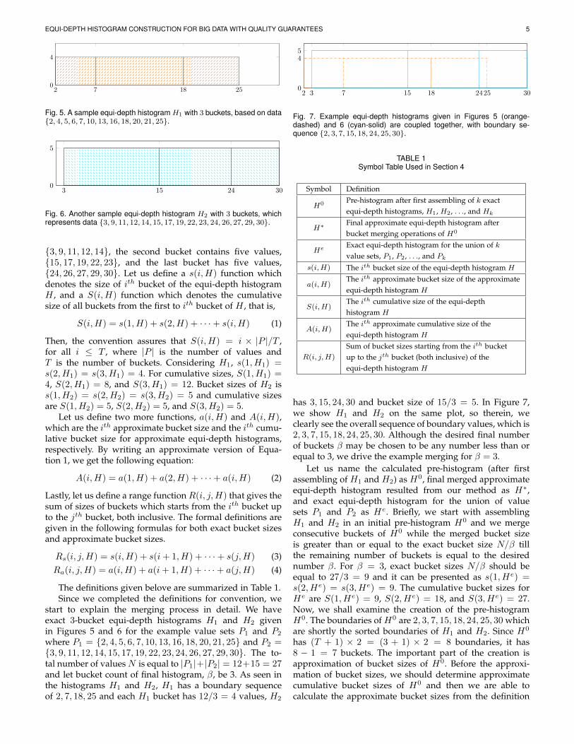
start to explain the merging process in detail. We haveexact 3-bucket equi-depth histograms H1 and H2 givenin Figures 5 and 6 for the example value sets P1 and P2

where P1 = {2, 4, 5, 6, 7, 10, 13, 16, 18, 20, 21, 25} and P2 ={3, 9, 11, 12, 14, 15, 17, 19, 22, 23, 24, 26, 27, 29, 30}. The to-tal number of valuesN is equal to |P1|+|P2| = 12+15 = 27and let bucket count of final histogram, β, be 3. As seen inthe histograms H1 and H2, H1 has a boundary sequenceof 2, 7, 18, 25 and each H1 bucket has 12/3 = 4 values, H2

2 3 7 15 18 2425 300

45

Fig. 7. Example equi-depth histograms given in Figures 5 (orange-dashed) and 6 (cyan-solid) are coupled together, with boundary se-quence {2, 3, 7, 15, 18, 24, 25, 30}.

TABLE 1Symbol Table Used in Section 4

Symbol Definition

H0 Pre-histogram after first assembling of k exactequi-depth histograms, H1, H2, . . ., and Hk

H∗ Final approximate equi-depth histogram afterbucket merging operations of H0

He Exact equi-depth histogram for the union of kvalue sets, P1, P2, . . ., and Pk

s(i,H) The ith bucket size of the equi-depth histogram H

a(i,H)The ith approximate bucket size of the approximateequi-depth histogram H

S(i,H)The ith cumulative size of the equi-depthhistogram H

A(i,H)The ith approximate cumulative size of theequi-depth histogram H

R(i, j,H)

Sum of bucket sizes starting from the ith bucketup to the jth bucket (both inclusive) of theequi-depth histogram H

has 3, 15, 24, 30 and bucket size of 15/3 = 5. In Figure 7,we show H1 and H2 on the same plot, so therein, weclearly see the overall sequence of boundary values, which is2, 3, 7, 15, 18, 24, 25, 30. Although the desired final numberof buckets β may be chosen to be any number less than orequal to 3, we drive the example merging for β = 3.

Let us name the calculated pre-histogram (after firstassembling of H1 and H2) as H0, final merged approximateequi-depth histogram resulted from our method as H∗,and exact equi-depth histogram for the union of valuesets P1 and P2 as He. Briefly, we start with assemblingH1 and H2 in an initial pre-histogram H0 and we mergeconsecutive buckets of H0 while the merged bucket sizeis greater than or equal to the exact bucket size N/β tillthe remaining number of buckets is equal to the desirednumber β. For β = 3, exact bucket sizes N/β should beequal to 27/3 = 9 and it can be presented as s(1, He) =s(2, He) = s(3, He) = 9. The cumulative bucket sizes forHe are S(1, He) = 9, S(2, He) = 18, and S(3, He) = 27.Now, we shall examine the creation of the pre-histogramH0. The boundaries of H0 are 2, 3, 7, 15, 18, 24, 25, 30 whichare shortly the sorted boundaries of H1 and H2. Since H0

has (T + 1) × 2 = (3 + 1) × 2 = 8 boundaries, it has8 − 1 = 7 buckets. The important part of the creation isapproximation of bucket sizes of H0. Before the approxi-mation of bucket sizes, we should determine approximatecumulative bucket sizes of H0 and then we are able tocalculate the approximate bucket sizes from the definition

EQUI-DEPTH HISTOGRAM CONSTRUCTION FOR BIG DATA WITH QUALITY GUARANTEES 6

2 3 7 15 18 2425 300

45

Fig. 8. The initial pre-histogram H0 constructed just after the first as-sembling of H1 and H2.

of the cumulative bucket size function A(i,H). The approx-imate cumulative bucket sizes are calculated by presumingthat all values in each bucket are at the beginning boundaryof the bucket. For example, let us consider the first bucketof H1. In this bucket, we have values 2, 4, 5, and 6 andwe suppose that all these values are at the point 2. Byusing this supposition, any cumulative bucket size is easilydetermined by summing the bucket size of the histogramwhich holds the next boundary and the previous cumulativebucket size starting with 0. Thus, since the first boundary ofH0 is 2 and this boundary is the first boundary of H1, thefirst cumulative approximate bucket size A(1, H0) is equalto s(1, H1) = 4. The second cumulative approximate bucketsize A(2, H0) is equal to s(1, H2) + A(1, H0) = 5 + 4 = 9because the next coming H0 boundary is 3 and it isthe first boundary of H2. After the boundary 3, the nextH0 boundary is 7 and it is the second boundary of H1.Therefore, the third cumulative approximate bucket sizeA(3, H0) is equal to s(2, H1) +A(2, H0) = 4 + 9 = 13. Theremaining approximate bucket sizes are calculated in thesame way and A(4, H0), A(5, H0), A(6, H0), and A(7, H0)are 18, 22, 27, and 27, respectively. Now, we are able tocalculate approximate bucket sizes. Approximate size of thefirst bucket a(1, H0) relying between boundary 2 and 3 isdirectly equal to A(1, H0) and it is 4. The second approx-imate bucket size a(2, H0) is the difference between thefirst and the second cumulative bucket size. Thus, a(2, H0)is equal to A(2, H0) − A(1, H0) = 9 − 4 = 5. Similarly,a(3, H0) = A(3, H0)−A(2, H0) = 13−9 = 4, a(4, H0) = 5,a(5, H0) = 4, a(6, H0) = 5, and a(7, H0) = 0. Graphicalrepresentation of created H0 is given in Figure 8.

Next, we merge the buckets of H0 until the remainingbucket count is equal to β. We use approximate cumulativebucket size instead of approximate bucket size to decreasethe division error while merging. The merging process startswith the first bucket of H0. First of all we compare thefirst cumulative bucket size of H0, A(1, H0), with the firstcumulative bucket size of exact (ideal) histogram, S(1, He),and we see that A(1, H0) is less than S(1, He). We continuecomparing the next cumulative bucket size of H0, A(2, H0),with again the first cumulative bucket size of exact (ideal)histogram, S(1, He), and we now see that A(2, H0) is equalto S(1, He). Again, we continue comparing. This time, wesee that A(3, H0) is greater than S(1, He).Therefore, thebuckets starting from the first bucket to the third bucketexcept the third one (because the result of the previouscomparison is equality) would be merged and this mergedbucket would be the first bucket of the final merged ap-proximate histogram, H∗. The resulting new bucket sizewould be A(2, H0) because the new merged bucket is thefirst bucket of H∗. Then, we are going to create the second

2 7 18 300

9

(a) The final approximate histogram H∗ constructed by merging H1 andH2.

2 12 21 300

9

(b) The exact histogram for union of P1 and P2.

Fig. 9. The final approximate and exact histograms of the example valuesets P1 and P2.

bucket of H∗. For this creation, we continue comparingcumulative bucket sizes starting from the first not mergedbucket number with the second cumulative bucket size ofHe. We see that A(3, H0) is less than S(2, He). Next com-parison is between the next cumulative of H0 and again thesecond cumulative ofHe. This time equality is seen. We con-tinue comparing the next cumulative of H0, A(5, H0) withS(2, He). At this point, A(5, H0) is greater than S(2, He).Thus, we merge the buckets starting from the third one tothe fifth one again except the fifth one and the created newbucket would be the second bucket of H∗. This mergingprocess would end when the remaining bucket count isequal to β and we getH∗ = {(2, 9), (7, 9), (18, 9), (30, 0)} asseen in Figure 9a. For comparison, He is given in Figure 9b.

The generalization of this method for merging more than2 histograms is now easy after the one given above. Let ushave k value sets (P1, P2, ..., Pk) and their summaries (T-bucket equi-depth histograms,H1,H2, ...,Hk) to be merged.The merging process for the general case starts with thecreation of an initial pre-histogram, H0. This can be donewith sorting all boundary values coming from summariesand determining approximate bucket sizes in the same waywith the one described above. The calculated histogramH0 has k × (T + 1) boundaries and thus k × (T + 1) − 1buckets. The rest of the merging method is exactly the samewith the case when we have only two histograms. Thatis, we combine consecutive buckets of H0 by comparingthe cumulative bucket sizes of H0 with cumulative sizes ofexact histogram, He, until β buckets remain.

Algorithm 1 shows the pseudocode of the explainedmethod above. The algorithm takes T -bucket equi-depthhistograms of k value sets, total number of values, N , which

EQUI-DEPTH HISTOGRAM CONSTRUCTION FOR BIG DATA WITH QUALITY GUARANTEES 7

Algorithm 1: Equi-depth Histogram MergingInput: H1, H2, . . . ,Hk: k equi-depth histograms each

with T buckets, N : total number of values, β:desired bucket count of final histogram

Output: H∗: an approximate equi-depth histogramwith β buckets.

1 b← {sorted boundaries of H1, H2, . . . ,Hk}2 s← {bucket sizes calculated as described}3 H0 ← CREATEHISTOGRAM(b, s)4 H∗ ← H0

5 last← 1; next← 1; current← 16 remaining← k(T + 1)− 17 while remaining > β do8 while A(next,H0) ≤ current×N/β do9 next← next+ 1

10 MERGEBUCKETS(last, next− 1, H∗)11 last← next; current← current+ 112 remaining← remaining − (next− 1− last)

13 return H∗

is the sum of all sizes of value sets, and desired bucketcount of final histogram, β as inputs and constructs andreturns final approximate β-bucket equi-depth histogram,H∗. Lines 1 through 3 of the algorithm is performed for thecreation of the initial pre-histogram,H0. First, boundaries ofinput histograms are sorted at Line 1 and then bucket sizesare calculated according to the above example at Line 2.The subroutine CREATEHISTOGRAM called at Line 3 simplycreates a histogram from given boundary and bucket sizesets and at that line H0 is created from b and s. The createdH0 has k× (T +1) boundaries and k× (T +1)− 1 buckets.After creation of H0, it would be copied to H∗ at Line 4.Once H0 is created and copied to H∗, required bucketsare combined on H∗ considering ideal bucket size, N/β.The main While loop iterates until the remaining numberof buckets is equal to β. The inner While loop given inLines 8 and 9 seeks for the next feasible point of bucketsto combine at each iteration of the main loop. When such apoint is found, we apply MERGEBUCKETS subroutine whichcombines buckets from last to next − 1, both inclusive,on H∗ as shown in Line 10. Notice that MERGEBUCKETSmerges buckets according to the first state of bucket indexes.

For the asymptotic performance of the algorithm, sortingboundaries is likewise merging k sorted lists and it can bedone in O(Tk log k). Bucket sizes and CREATEHISTOGRAMsubroutine can both run in O(Tk) at Lines 2 and 3. For theinner loop, the increment at Line 9 can be performed at mostβ times. The number of iterations for the main loop changeswith the decrease in remaining bucket counts. Observe thatthe decrease is equal to the inner loop iteration number andMERGEBUCKETS subroutine takes the same time with theinner loop for each main loop iteration. Considering thisobservation, total time required for the main loop is O(Tk).Consequently, the initial sorting dominates the rest of thealgorithm, and the algorithm runs in O(Tk log k)-time.

Let us debug the algorithm line by line for the twoexample 3-bucket equi-depth histograms H1 and H2

given in Figures 5 and 6. Recall that H1 and H2 are

2 3 7 15 18 2425 300

4

5

9

Fig. 10. The state of H∗ after the first iteration of main loop of 1.

histograms of value sets P1 and P2. Therefore N is equal to|P1|+|P2| = 12+15 = 27. Let β is equal to 3. We knowH0 ={(2, 4), (3, 5), (7, 4), (15, 5), (18, 4), (24, 5), (25, 0), (30, 0)}from the given detailed explanation above. In addition, thestart state of H∗ is the same as H0. The variables last, next,and current is equal to 1 and remaining is calculated ask(T + 1) − 1 = 2(3 + 1) − 1 = 7. Because the remainingis greater than β at current state, we enter the main loop.For the inner loop, A(1, H0) and A(2, H0) is less or equalto current × N/β which is 1 × 27/3 = 9 but A(3, H0) isgreater than 9. Hereby, inner While loop 2 times and nextwould be 3. Then, MERGEBUCKETS subroutine merges thebuckets 1 and 2 of H∗. The illustration of H∗ is shown inFigure 10 after merging. The variables last and currentare updated after the execution of MERGEBUCKETS isfinished and last would be 3 and current would be 2.The remaining variable, keeping the remaining bucketnumber of H∗, would be 6 after the calculation is done atLine 12. The main loop finishes after H∗ has β buckets andexecution of the algorithm ends with returning the createdH∗.

Now, we discuss the error bounds of the output his-togram H∗. The following two theorems and their proofsverify the error bounds on bucket sizes and the sum of anyrange of bucket sizes of H∗.

Theorem 1. Let H1, H2, . . . , Hk be T -bucket equi-depthhistograms of value sets P1, P2, . . . , Pk, and H∗ bethe approximate β-bucket equi-depth histogram whereβ ≤ T constructed by the algorithm. Then, the size ofany bucket a(i,H∗) is (N/β) ± εmax where εmax <2β/T × (N/β).

Proof 1. Recall that the calculations of bucket sizes of H0

depends on supposition that all values in each bucketare at the beginning boundary of the bucket and H∗ issome-buckets-merged version of H0. Now consider anith bucket between the ith and the i+ 1th boundaries(boundaries may be any of the two consecutive bound-aries of H0) of H∗ illustrated in Figure 11. As seen inthe figure, all of the values in the buckets divided bythe ith boundary may stay at the right hand side of theboundary in contrast to our assumption and all values inthe buckets divided by the i+ 1th boundary may stay atthe left hand side of the boundary. In this case, a(i,H∗)gets the maximum value. Vice versa, a(i,H∗) gets theminimum value in the case that all possible values inthe divided buckets stay out of the ith bucket in contrast

EQUI-DEPTH HISTOGRAM CONSTRUCTION FOR BIG DATA WITH QUALITY GUARANTEES 8

Fig. 11. Illustration of maximum bucket size.

to the case seen in Figure 11. The following calculationshows the maximum value of a(i,H∗).

a(i,H∗)max = C + |P1|/T + |P3|/T+ · · ·+ |Pk|/T+ |P1|/T + |P2|/T+ · · ·+ |Pk−1|/T (5)

where C is constant which is the sum of the sizes of thebuckets relying completely in the ith bucket and |P1|,|P2|, . . . , |Pk| is the size of sets. Adding and subtracting|P2|/T and |Pk|/T to the equation, we get the followingequation.

a(i,H∗)max = C + (|P1|+ |P2|+ · · ·+ |Pk|)/T+ (|P1|+ |P2|+ · · ·+ |Pk|)/T− |P2|/T − |Pk|/T

= C + 2N/T − |P2|/T − |Pk|/T< C + 2N/T (6)

And a(i,H∗)min is equal to C because no additionalvalues are located in the ith bucket except the constantones. Once a(i,H∗)max and a(i,H∗)min are determined,εmax would be the difference between them.

εmax = a(i,H∗)max − a(i,H∗)min

< C + 2N/T − C< 2N/T (7)

The following equation shows another expression ofεmax in terms of exact (ideal) bucket size N/β.

εmax = 2N/T

< 2Nβ/Tβ

< 2β/T × (N/β) (8)

Theorem 2. Let H1, H2, . . . , Hk be T -bucket equi-depthhistograms of value sets P1, P2, . . . , Pk, and H∗ bethe approximate β-bucket equi-depth histogram whereβ ≤ T constructed by the algorithm. Then, the sizeof any range spanning m buckets, Ra(i, i + m,H∗), ism× (N/β)± εmax where εmax < 2β/T × (N/β).

Proof 2. Let us start with proving the error bound ofrange size of two consecutive buckets. Figure 12 shows

Fig. 12. Illustration of maximum size of a range of buckets.

this case. There are two consecutive buckets and threeboundaries (bi, bi+1, and bi+2), the middle one (bi+1)splits the two buckets. Notice that the intersected bucketsby bi+1 completely rely in the range of the two bucketsand this means that the sizes of these buckets are addedas a constant to the range sizeRa(i, i+1, H∗). As a result,this proof turns into the proof of error bound of bucketsize given in Proof 1 and Equation 7 and Equation 7 alsoproves Theorem 2. The general case -spanning rangesincludes more than two buckets- can also transform intoa single bucket problem in the same way with the casewith two buckets.

According to Theorems 1 and 2, users can bound themaximum bucket size error of final β-bucket approximateequi-depth histogram H∗ by selecting appropriate bucketnumbers β and T . For example, let us calculate T , numberof buckets of equi-depth histograms of data partitions keptin the summary files, in terms of β for getting final mergedhistograms, the maximum bucket size errors of which donot exceed 5% of the ideal bucket size (N/β). If we useEquation 8, we can find the minimum number of bucketsT needed to satisfy the 5% error condition as follows.

εmax < 2β/T × (N/β) ≤ 0.05(N/β)

40β ≤ T

Consequently, the required bucket size T should be at least40 times β which is the desired number of buckets ofconstructed histograms using our method.

5 IMPLEMENTATION WITH HADOOP MAP-REDUCE

In this section, we explain the implementation details of ourhistogram processing framework on Hadoop MapReduce.The framework consists of two main MapReduce jobs. Oneof them is named as Summarizer which runs offline andis scheduled for summarizing the new coming data toHDFS. The Summarizer constructs a T -bucket equi-depthhistogram of the data. After summarizing, the resultingequi-depth histograms are stored in HDFS. The second job,Merger, is run on-demand according to users’ requests. Itsduty is to merge the related summaries from HDFS byconsidering user requests and to construct the final β-bucketapproximate equi-depth histogram.

EQUI-DEPTH HISTOGRAM CONSTRUCTION FOR BIG DATA WITH QUALITY GUARANTEES 9

Fig. 13. Overview of Proposed Framework

The overview picture of the histogram processing frame-work is given in Figure 13. In the left of the figure, HDFSholds whole data including the new data, summary files,and created histograms according to user requests. Theframework is in the right of the picture and Summarizerand Merger jobs take place in the framework. Every time,new data is pushed to HDFS, the Summarizer constructs itssummary (T -bucket equi-depth histogram) and saves it toHDFS, again. When a user requests an equi-depth histogramof desired partitions (it can be any set of data partitions),the Merger processes the request by merging the relatedsummaries of desired partitions and saves the merged finalhistogram to HDFS. These jobs can also be implemented inthe Hive and Pig as user functions.

6 RELATED WORK

Basically, histograms are used to get quick distribution ofinformation from the given data. This quick information isused especially in database systems in computer science e.g.selectivity estimation to optimize queries, load balancingof join queries, and much more [24]. There are differenttypes of histograms and each type of histogram has differentproperties [31]. Exact histogram construction is not feasiblewhen the data is too big or the data is frequently updated.In such cases, histograms are constructed from sampled dataand/or maintained according to the updated data [32]. Thistype of histograms are called approximate histograms ratherthan exact histograms. Approximate histogram constructionfrom sampled data can be divided into two categories bysampling method [33] which are tuple-level sampling andblock-level sampling. Tuple-level sampling method usesuniform-random-sampling to sample the data at tuple levelto construct an approximate histogram at the desired error

bound [34], [35]. Gibbons et al. [34] proposed a sampling-based incremental maintenance approach of approximatehistograms. The proposed approach, backing sample, keepsthe sampled tuples up-to-date in a relation. A bound of theamount of the sampling size for a given error bound studiedby Chaudhuri et al. [35] in addition to proposing an adap-tive page sampling algorithm. The second method, block-level sampling, exemplifies the data according to an iterativecross-validation based approach [36], [37]. Chaudhuri etal. [37] proposed a method for approximate histogram con-struction using an initial set of data and iteratively updatedthe constructed histogram until the histogram error is underthe predetermined level. All of the proposed approachesabove, however, are for single-node databases.

When the data is too big to handle in a single-nodedatabase, the data is distributed to multi-nodes. One ofthe well-known distributed data storage frameworks isHadoop Distributed File System (HDFS) [30] and the dataprocessing framework of the stored data in the HDFS isHadoop MapReduce [5]. The histogram construction of suchdistributed data is not well-studied and there is less workon histogram creation of distributed data than the oneson undistributed data. One of the adapted methods forcontructing approximate histogram is tuple-level sampling.Okcan et al. [15] proposed a tuple-level sampling basedalgorithm to construct approximate equi-depth histogramsfor distributed data to improve processing theta-joins usingMapReduce. The algorithm works as follows. In the mapsection of a MapReduce Job, a predefined number of tuplesare selected randomly by scanning the whole data andoutputted. The tuples are sorted and sent to the reducer. Thereducer of the job determines and outputs the boundariesof equi-depth histograms. In [38], a method for approx-imate wavelet histogram construction for big data usingMapReduce is proposed and an improved sampling method-ignoring low frequent sampled keys in splits- is given. Thedrawback of such histogram construction algorithms of dis-tributed data using tuple-level sampling is that scanning thewhole data is a time consuming process. Another approxi-mate histogram construction method is proposed in [33].This method also uses a sampling method named two-phasesampling which samples the whole data at block-level andconstructs the approximate histogram and calculates theerror. If the error is not in the desired error boundary, theadditional sampling size needed is calculated and histogramconstruction process is repeated. The insufficiency of thismethod is that histogram is rebuilt for every new dataand it requires a customized MapReduce framework. Inthis paper, we propose a novel approximate equi-depthhistogram construction method with a log histogram mon-itoring framework that users can query the daily storedlog files for their equi-depth histogram. In the proposedmethod, a MapReduce Job is scheduled to summarize thedaily stored log files which means that the exact equi-depth histogram of each log file is constructed and stored incorresponding summary files and another MapReduce Jobmerges the summaries of intended log files for approximateequi-depth histogram construction.

EQUI-DEPTH HISTOGRAM CONSTRUCTION FOR BIG DATA WITH QUALITY GUARANTEES 10

7 EXPERIMENTAL RESULTS

In this section, we will describe how we tested the pro-posed method. The method was implemented on HadoopMapReduce framework and was tested on two differentdatasets. One of them is synthetic data with 155 million oftuples created by using Gumbel distribution for skewnessto represent the response of the method for skewed data.The other one is 295 GB uncompressed real data which istaken from hourly page view statistics of Wikipedia. Thedata consists of approximately 5 billion tuples which belongto January 2015 and each tuple has 4 columns which arelanguage, pagename, pageviews and pagesize. We usedpagesize for histogram construction. The proposed method(merge) is compared with corrected tuple level randomsampling (tuple). By definition, bare tuple level randomsampling collects tuples randomly and constructs histogramwith collected tuples but doing so does not work well whenthe data is sparse at the edges. Therefore, we fix this problemby including the edge values to the collected tuples by de-fault. As mentioned in Subsection 2, histogram constructionof the data coming from daily logs is an important issue andtuple level random sampling method is also unfavorable forconstructing a histogram of a given time interval. Hereby,sampling stage of tuple level is run offline to compare timespendings.

All equi-depth histograms are build with bucket size of254 as used by Oracle as default bucket size for histogramenhancement. We fundamentally run two types of tests torepresent the effectiveness of the proposed method in termsof boundary and bucket size error and run time. The firsttest represents the results according to T changes which isdaily exact histogram bucket size for the proposed methodand sample size for tuple level sampling. The second testrepresents the run time efficiency of histogram constructionfor the changes in a given time interval.

Approximate histograms may have two types of error.One of them is that approximate histograms may not havethe same bucket boundaries with the exact ones and theother is that bucket sizes of the approximate histograms maydeviate from the exact ones. The former error is named asboundary error (µb) and defined as follows:

µb =B

vmax − vmin

√√√√ 1

B + 1

B+1∑i=1

[b(i,H∗)− b(i,H)]2. (9)

where B is the bucket size, vmax and vmin are maximumand minimum values in relation R respectively, and thefunction b(i,H) is the ith value of a given histogram H .µb is the standard deviation of boundary errors normalizedwith respect to the mean boundary length (vmax−vmin)/B.The latter error is named as size error (µs) and formulatedas follows:

µs =B

N

√√√√ 1

B

B∑i=1

[s(i,H∗)− s(i,H)]2. (10)

where N is the total number of elements in relation R andfunction s(i,H) is the size of the ith bucket of a givenhistogram H . s(i,H) is equal to the mean bucket size N/Bfor all i values in the range of 1 to B if the given histogram

(a) Graph of µb against T for real data

(b) Graph of µs against T for real data

Fig. 14. Lin-log graphs of error metrics against T (B × 254× 2n) whichis summary size in merge method and sampling size in tuple for realdata

H is an equi-depth histogram. µs is the standard deviationof bucket size errors normalized with respect to the meanbucket size N/B.

7.1 Effect of TChanging T value effects the accuracy of the constructedapproximate equi-depth histogram. The first experiment isrun to show the effects of T changes on both the proposedmethod and tuple level sampling. Figures 14 and 15 showthe error graphs of the approximate equi-depth histogramsconstructed using the proposed method and tuple levelsampling method. According to the graph in Figure 14a,the constructed histogram by using merge method for realdata is at least 2 times more accurate in terms of boundaryerror µb than the one constructed using tuple method.Moreover, the µb error for tuple method is not consistentbecause of the randomness and the construction processmust be repeated for consistency and this is not convenientbecause of the run time. For example, let us consider thegraph of µb against T given in Figure 14a. Notice that theµb error for tuple method is not consistent. The expectedresult is that µb should decrease while T increases. On theother hand, it is clearly seen from the graphs of mergemethod in Figures 14a, 14b, 15a, and 15b that µb is a non-decreasing function of T . The reason of this consistency is

EQUI-DEPTH HISTOGRAM CONSTRUCTION FOR BIG DATA WITH QUALITY GUARANTEES 11

(a) Graph of µb against T for skewed data

(b) Graph of µs against T for skewed data

Fig. 15. Lin-log graphs of error metrics against T (B×254×2n) which issummary size in merge method and sampling size in tuple for skeweddata

the maximum error bound of merge method described inSection 4 in detail. The mean running times for all methodsare given in Table 2. Run times for merging daily summariesand samplings are nearly the same. But required time for thesummarization stage ofmergemethod is more than the timefor offline sampling stage of tuple method. The reason ofthis time difference is that summarization is exact histogramconstruction and exact histogram construction for each datapartition requires a complete MapReduce Job with a mapperand a reducer and the data comes from each mapper sub-jected to shuffle and sort phase. On the other hand, tuplelevel random sampling does not require a reducer becausethe randomly selected tuples would be stored directly with-out sorting. Because of this difference, summarization ofeach day for real data takes approximately 12 minutes whilesampling takes 4 minutes. Although this time efficiency oftuple method, all the daily summarizations and samplingsare done offline, it makes merge method convenient for reallife applications.

7.2 Effect of given time interval

Histogram constructions according to the given time in-terval effect deviation of approximate histograms from theexact ones and running times. We compared merge method

(a) Graph of µb against merged # of days for real data

(b) Graph of µs against merged # of days for real data

Fig. 16. Graphs of error metrics against merged # of days for real data

with tuple method with an experiment for 5 different timeintervals (1 day, 1 week, 2 weeks, 3 weeks, and 1 month).T value is taken to be B × 254 × 212 for real data and tobe B × 254× 27 for skewed data. All daily exact histogramand samplings are computed offline. In Figures 16 and 17,graphs of error metrics against time intervals are given andit is clearly seen from the graphs that the proposed methodproduces more sensible histograms than the ones producedusing tuple level random sampling. In particular, a real datahistogram constructed using merge method has at least 10times less boundary error than the one constructed usingtuple method in Figure 16a. Besides, again the consistencyis an issue for tuple method as seen in Figures 16a and 17a.The graphs of running time against number of days aregiven in Figure 18. More specifically, the compared methods(merge and tuple) run in nearly the same time durationexcept offline parts.

8 CONCLUSION

In this paper, we proposed a novel approximate equi-depthhistogram construction method by merging precomputedexact equi-depth histograms of data partitions. The methodis implemented on Hadoop to demonstrate how it is appliedto real life problems. The theoretical calculations and theexperimental results showed that both the bucket size errorsand total size error of any bucket range are bounded by

EQUI-DEPTH HISTOGRAM CONSTRUCTION FOR BIG DATA WITH QUALITY GUARANTEES 12

(a) Graph of µb against merged # of days for skewed data

(b) Graph of µs against merged # of days for skewed data

Fig. 17. Graphs of error metrics against merged # of days for skeweddata

TABLE 2Mean Running Times of Monthly Equi-depth Histogram Construction

Method Real Data Skewed DataExact Hist. Construction 24358 582Tuple with Online Sampling 6169 68Summarizing for Each Day 725 18Merging of Daily Summaries 117 73Sampling for Each Day 223 18Merging of Daily Samplings 113 71

a predefined error set by a user in terms of T and β. Inparticular, the experimental results run on both real andsynthetic data show that the constructed histograms usingthe proposed method (merge) are more accurate than thetuple level random sampling (tuple) with a cost of offlinerun time. In addition to the proposed merged based his-togram construction method, we also proposed a novel his-togram processing framework for the daily stored log files.This framework is crucial for fast histogram constructionover a subset of a list of partitions on demand. The timecomplexity and the incrementally updated nature of theproposed method makes it practical to be applied over reallife problems.

(a) Running time against merged # of days for real data

(b) Running time against merged # of days for skewed data

Fig. 18. Graphs of running time against merged # of days

ACKNOWLEDGMENTS

We would like to thank Enver Kayaaslan for his help forpresentation.

REFERENCES

[1] D. Logothetis, C. Olston, B. Reed, K. C. Webb, and K. Yocum,“Stateful bulk processing for incremental analytics,” in Proceedingsof the 1st ACM symposium on Cloud computing. ACM, 2010, pp.51–62.

[2] A. Thusoo, Z. Shao, S. Anthony, D. Borthakur, N. Jain,J. Sen Sarma, R. Murthy, and H. Liu, “Data warehousing andanalytics infrastructure at facebook,” in Proceedings of the 2010ACM SIGMOD International Conference on Management of data.ACM, 2010, pp. 1013–1020.

[3] A. Thusoo, J. S. Sarma, N. Jain, Z. Shao, P. Chakka, N. Zhang,S. Antony, H. Liu, and R. Murthy, “Hive-a petabyte scale datawarehouse using hadoop,” in Data Engineering (ICDE), 2010 IEEE26th International Conference on. IEEE, 2010, pp. 996–1005.

[4] A. S. Foundation. (2008) Apache hadoop. [Online]. Available:https://hadoop.apache.org/

[5] J. Dean and S. Ghemawat, “Mapreduce: a flexible data processingtool,” Communications of the ACM, vol. 53, no. 1, pp. 72–77, 2010.

[6] J. Dittrich, J.-A. Quiane-Ruiz, A. Jindal, Y. Kargin, V. Setty, andJ. Schad, “Hadoop++: making a yellow elephant run like a cheetah(without it even noticing),” Proceedings of the VLDB Endowment,vol. 3, no. 1-2, pp. 515–529, 2010.

[7] A. F. Gates, O. Natkovich, S. Chopra, P. Kamath, S. M. Narayana-murthy, C. Olston, B. Reed, S. Srinivasan, and U. Srivastava,“Building a high-level dataflow system on top of map-reduce: thepig experience,” Proceedings of the VLDB Endowment, vol. 2, no. 2,pp. 1414–1425, 2009.

EQUI-DEPTH HISTOGRAM CONSTRUCTION FOR BIG DATA WITH QUALITY GUARANTEES 13

[8] A. Jindal, J.-A. Quiane-Ruiz, and J. Dittrich, “Trojan data layouts:right shoes for a running elephant,” in Proceedings of the 2nd ACMSymposium on Cloud Computing. ACM, 2011, p. 21.

[9] M. Zaharia, A. Konwinski, A. D. Joseph, R. H. Katz, and I. Stoica,“Improving mapreduce performance in heterogeneous environ-ments.” in OSDI, vol. 8, no. 4, 2008, p. 7.

[10] M. Isard, M. Budiu, Y. Yu, A. Birrell, and D. Fetterly, “Dryad: dis-tributed data-parallel programs from sequential building blocks,”in ACM SIGOPS Operating Systems Review, vol. 41, no. 3. ACM,2007, pp. 59–72.

[11] A. Floratou, J. M. Patel, E. J. Shekita, and S. Tata, “Column-oriented storage techniques for mapreduce,” Proceedings of theVLDB Endowment, vol. 4, no. 7, pp. 419–429, 2011.

[12] Y. Lin, D. Agrawal, C. Chen, B. C. Ooi, and S. Wu, “Llama:leveraging columnar storage for scalable join processing in themapreduce framework,” in Proceedings of the 2011 ACM SIGMODInternational Conference on Management of data. ACM, 2011, pp.961–972.

[13] F. N. Afrati and J. D. Ullman, “Optimizing joins in a map-reduceenvironment,” in Proceedings of the 13th International Conference onExtending Database Technology. ACM, 2010, pp. 99–110.

[14] S. Blanas, J. M. Patel, V. Ercegovac, J. Rao, E. J. Shekita, andY. Tian, “A comparison of join algorithms for log processing inmapreduce,” in Proceedings of the 2010 ACM SIGMOD InternationalConference on Management of data. ACM, 2010, pp. 975–986.

[15] A. Okcan and M. Riedewald, “Processing theta-joins using mapre-duce,” in Proceedings of the 2011 ACM SIGMOD International Con-ference on Management of data. ACM, 2011, pp. 949–960.

[16] J.-A. Quiane-Ruiz, C. Pinkel, J. Schad, and J. Dittrich, “Raftingmapreduce: Fast recovery on the raft,” in Data Engineering (ICDE),2011 IEEE 27th International Conference on. IEEE, 2011, pp. 589–600.

[17] S. Wu, F. Li, S. Mehrotra, and B. C. Ooi, “Query optimization formassively parallel data processing,” in Proceedings of the 2nd ACMSymposium on Cloud Computing. ACM, 2011, p. 12.

[18] S. Babu, “Towards automatic optimization of mapreduce pro-grams,” in Proceedings of the 1st ACM symposium on Cloud com-puting. ACM, 2010, pp. 137–142.

[19] H. Herodotou and S. Babu, “Profiling, what-if analysis, and cost-based optimization of mapreduce programs,” Proceedings of theVLDB Endowment, vol. 4, no. 11, pp. 1111–1122, 2011.

[20] E. Jahani, M. J. Cafarella, and C. Re, “Automatic optimization formapreduce programs,” Proceedings of the VLDB Endowment, vol. 4,no. 6, pp. 385–396, 2011.

[21] D. Jiang, B. C. Ooi, L. Shi, and S. Wu, “The performance of mapre-duce: An in-depth study,” Proceedings of the VLDB Endowment,vol. 3, no. 1-2, pp. 472–483, 2010.

[22] J. Dittrich, J.-A. Quiane-Ruiz, S. Richter, S. Schuh, A. Jindal, andJ. Schad, “Only aggressive elephants are fast elephants,” Proceed-ings of the VLDB Endowment, vol. 5, no. 11, pp. 1591–1602, 2012.

[23] Yahoo advertising. [Online]. Available: https://advertising.yahoo.com/yahoo-sites/Homepage/index.htm

[24] Y. Ioannidis, “The history of histograms (abridged),” in Proceedingsof the 29th international conference on Very large data bases-Volume 29.VLDB Endowment, 2003, pp. 19–30.

[25] P. M. Hallam-Baker and B. Behlendorf, “Extended log file format,”WWW Journal, vol. 3, p. W3C, 1996.

[26] S. Ghemawat, H. Gobioff, and S.-T. Leung, “The google filesystem,” in ACM SIGOPS operating systems review, vol. 37, no. 5.ACM, 2003, pp. 29–43.

[27] J. Dean and S. Ghemawat, “Mapreduce: simplified data processingon large clusters,” Communications of the ACM, vol. 51, no. 1, pp.107–113, 2008.

[28] C. Olston, B. Reed, U. Srivastava, R. Kumar, and A. Tomkins, “Piglatin: a not-so-foreign language for data processing,” in Proceedingsof the 2008 ACM SIGMOD international conference on Management ofdata. ACM, 2008, pp. 1099–1110.

[29] A. Thusoo, J. S. Sarma, N. Jain, Z. Shao, P. Chakka, S. Anthony,H. Liu, P. Wyckoff, and R. Murthy, “Hive: a warehousing solutionover a map-reduce framework,” Proceedings of the VLDB Endow-ment, vol. 2, no. 2, pp. 1626–1629, 2009.

[30] D. Borthakur, “Hdfs architecture guide,” HADOOP APACHEPROJECT http://hadoop. apache. org/common/docs/current/hdfs design.pdf, 2008.

[31] V. Poosala, P. J. Haas, Y. E. Ioannidis, and E. J. Shekita, “Improvedhistograms for selectivity estimation of range predicates,” in ACMSIGMOD Record, vol. 25, no. 2. ACM, 1996, pp. 294–305.

[32] A. C. Gilbert, S. Guha, P. Indyk, Y. Kotidis, S. Muthukrishnan,and M. J. Strauss, “Fast, small-space algorithms for approximatehistogram maintenance,” in Proceedings of the thiry-fourth annualACM symposium on Theory of computing. ACM, 2002, pp. 389–398.

[33] Y.-J. Shi, X.-F. Meng, F. Wang, and Y.-T. Gan, “Hedc++: Anextended histogram estimator for data in the cloud,” Journal ofComputer Science and Technology, vol. 28, no. 6, pp. 973–988, 2013.

[34] P. B. Gibbons, Y. Matias, and V. Poosala, “Fast incremental main-tenance of approximate histograms,” in VLDB, vol. 97, 1997, pp.466–475.

[35] S. Chaudhuri, R. Motwani, and V. Narasayya, “Random samplingfor histogram construction: How much is enough?” in ACMSIGMOD Record, vol. 27, no. 2. ACM, 1998, pp. 436–447.

[36] ——, “Histogram construction using adaptive random samplingwith cross-validation for database systems,” 2001, uS Patent6,278,989.

[37] S. Chaudhuri, G. Das, and U. Srivastava, “Effective use of block-level sampling in statistics estimation,” in Proceedings of the 2004ACM SIGMOD international conference on Management of data.ACM, 2004, pp. 287–298.

[38] J. Jestes, K. Yi, and F. Li, “Building wavelet histograms on largedata in mapreduce,” Proceedings of the VLDB Endowment, vol. 5,no. 2, pp. 109–120, 2011.

Burak Yıldız received his BS degree in mechan-ical engineering and MS degree in computerengineering from TOBB University of Economicsand Technology in 2013 and 2016, respectively.Large scale data management and data miningare in his major interest area.

Tolga Buyuktanır got his BS degree in com-puter engineering from Erciyes University in2014. He is now a master student at Turgut OzalUniversity in computer science. His research ar-eas include data mining and IoT.

Dr. Fatih Emekci got his MS and PhD from theDepartment of Computer Science at the Univer-sity of California, Santa Barbara in 2006. He wasat Oracle working with query optimizer team andat Linkedin working on data scalability problemsuntil 2012. He has been an associated professorof computer science at Turgut Ozal University,Ankara, Turkey since 2013.