EPA-454/R-92-006 (Revised) User's Guide to CAL3QHC · PDF fileA Modeling Methodology for...
124
EPA-454/R-92-006 (Revised) User's Guide to CAL3QHC Version 2.0: A Modeling Methodology for Predicting Pollutant Concentrations Near Roadway Intersections U.S. Environmental Protection Agency Office of Air Quality Planning and Standards Research Triangle Park, NC 27711 September, 1995
Transcript of EPA-454/R-92-006 (Revised) User's Guide to CAL3QHC · PDF fileA Modeling Methodology for...

EPA-454/R-92-006 (Revised) User's Guide to CAL3QHC Version 2.0: A Modeling Methodology for Predicting Pollutant Concentrations Near Roadway Intersections U.S. Environmental Protection Agency Office of Air Quality Planning and Standards Research Triangle Park, NC 27711 September, 1995

ii
DISCLAIMER This report has been reviewed by the Office of Air Quality Planning and Standards, U.S. Environmental Protection Agency and has been approved for publication. Any mention of trade names or commercial products is not intended to constitute endorsement or recommendation for use.

iii
PREFACE The CAL3QHC Version 2.0 model has been slightly revised. The revisions to the model are reflected in this version of the user's guide. The CAL3QHC Version 2.0 input structure has been converted from a "fixed format" to a "free format". Also, the CAL3QHC source code has been enhanced to permit the calculating of Particulate Matter (PM) concentrations. These revisions to CAL3QHC Version 2.0 will not change previous model results.

iv
TABLE OF CONTENTS Page PREFACE............................................................................................................ iii LIST OF FIGURES............................................................................................... vi LIST OF TABLES................................................................................................ viii ACKNOWLEDGEMENTS ...................................................................................... ix 1 INTRODUCTION............................................................................................. 1 2 BACKGROUND.............................................................................................. 3 3 MODEL DESCRIPTION.................................................................................... 7 3.1 Overview .............................................................................................. 7 3.2 Site Geometry ....................................................................................... 7 3.2.1 Free Flow Links ....................................................................... 9 3.2.2 Queue Links............................................................................ 9 3.2.3 Receptor Locations................................................................ 11 3.3 Emission Sources.................................................................................. 11 3.3.1 Free Flow Links ...................................................................... 12 3.3.2 Queue Links........................................................................... 13 3.4 Queuing Algorithm .............................................................................. 15 3.4.1 Overview............................................................................... 15 3.4.2 Queue Estimation for Under-Saturated Conditions ..................... 19 3.4.3 Queue Estimation for Over-Saturated Conditions ....................... 21 3.5 Dispersion Component .......................................................................... 24 3.6 Future Research Areas........................................................................... 24 4 USER INSTRUCTIONS................................................................................... 27 4.1 Data Requirements ............................................................................... 27 4.2 Limitations and Recommendations ........................................................ 28 4.3 Input Description.................................................................................. 32

v
TABLE OF CONTENTS (Continued) Page 4.4 Run Procedure...................................................................................... 39 4.5 Output Description ............................................................................... 39 4.6 Examples ............................................................................................. 40 4.6.1 Example 1: Two-way Signalized Intersection (Under-Capacity) .................................................................... 41 4.6.2 Example 2: Two-way Multiphase Signalized Intersection (Over-Capacity)..................................................... 41 4.6.3 Example 3: Urban Highway..................................................... 42 5 SENSITIVITY ANALYSIS ................................................................................. 73 5.1 Overview .............................................................................................. 73 5.2 Signal Timing........................................................................................ 75 5.3 Traffic Volume on the Queue Link ........................................................... 75 5.4 Traffic Lanes in the Queue Link............................................................... 78 5.5 Traffic Parameters.................................................................................. 78 6 MODEL VALIDATION ..................................................................................... 81 6.1 Overview .............................................................................................. 81 6.2 The New York City Database .................................................................. 81 6.3 Modeling Methodology .......................................................................... 82 6.4 Model Evaluation Results ....................................................................... 83 6.4.1 Regulatory Default Analysis...................................................... 83 6.4.2 Scoring Scheme Results........................................................... 83 References.................................................................................................... 89

vi
LIST OF FIGURES Figure Title and Description Page 1 Flowchart for CAL3QHC routines ...................................................... 8 2 Link and receptor geometry ............................................................. 10 3 Flowchart for queue link calculations................................................. 16 4 Queue and delay relationships for a near-saturated signalized intersection...................................................................... 18 5 Queue and delay relationships for an over-saturated signalized intersection...................................................................... 22 6 Example 1: Geometric configuration for a two-way intersection (units are in feet) ........................................................... 43 7 Example 2: Geometric configuration for a two-way multiphase intersection (units are in meters)....................................... 52 8 Example 3: Geometric configuration for an urban highway (units are in feet)................................................................ 64 9 Sensitivity analysis example run ........................................................ 74 10a Variation of CO concentrations (ppm) at receptor 1
(corner) versus wind angle for three different values of signal timing: 30% red time (V/C = 0.75, queue = 5.6), 40% red time (V/C = 0.88, queue = 9.0), and 50% red time (V/C = 1.08, queue = 42.9)............................. 76
10b Same as Figure 10a except at receptor 2 (mid-block) ........................... 76 11a Variation of CO concentrations (ppm) at receptor 1
(corner) versus wind angle for three different values of approach traffic volume: 1000 vph (V/C = 0.59, queue = 5.0), 1500 vph (V/C = 0.88, queue = 9.0), and 2000 vph (V/C = 1.18, queue = 93.5) ..... 77
11b Same as Figure 11a except at receptor 2 (mid-block) ........................... 77

vii
LIST OF FIGURES (Continued) Figure Title and Description Page 12a Variation of CO concentrations (ppm) at receptor 1
(corner) versus wind angle for different number of traffic lanes: two traffic lanes (V/C = 0.88, queue = 9.0) and three traffic lanes (V/C = 0.59, queue = 5.0).......................................................................... 79
12b Same as Figure 12a except at receptor 2 (mid-block) ........................... 79 13 The composite model comparison measure (CM) with 95%
confidence limits using CPM statistics............................................... 87 14 CM with 95% confidence limits using the AFB of
scientific category 1 ........................................................................ 88

viii
LIST OF TABLES Table Title and Description Page 1 Surface Roughness for Various Land Uses.......................................... 30 2 Description of Type of Variables ....................................................... 38 3 Example-1: Two way Signalized Intersection (Under-Capacity) ............................................................................. 44 4 Example-2: Two way Multiphase Signalized Intersection (Over-Capacity) ............................................................................... 53 5 Example-3: Urban Highway.............................................................. 65 6 Comparison of Top-Ten Observed Concentrations with
CAL3QHC Predicted Concentrations ................................................. 84

ix
ACKNOWLEDGEMENTS
Peter Eckhoff of EPA has revised the CAL3QHC Version 2.0 model and user's guide to
allow input data in "free format" and to allow for the analysis of Particulate Matter
(PM) impacts.
The original CAL3QHC Version 2.0 User's Guide was prepared for the United States
Environmental Protection Agency (EPA), Office of Air Quality Planning and Standards
(OAQPS) under contract No. 68-D90067. The authors, Guido Schattanek and June
Kahng, would like to express special acknowledgements to the EPA technical director,
Thomas N. Braverman, for his guidance and assistance in resolving technical issues, and
to Donald C. DiCristofaro of Sigma Research Corporation, Concord, Massachusetts, for
his contribution to the update of Chapters 4, 5, and 6, and the overall compilation of
the report.
The initial User's Guide to CAL3QHC was prepared in 1990 for the EPA/OAQPS under
Contract No. 68-02-4394 by the authors at Parsons Brinckerhoff Quade & Douglas, Inc.
in New York, New York. Special acknowledgements for their contribution to the initial
report are given to Thomas Wholley who provided the first concept of CAL3Q and
offered technical guidance; George Schewe (Environmental Quality Management) for
his assistance and direction in this effort; John Sun (Bechtel/Parsons Brinckerhoff)
whose initial recommendations led to the use of Highway Capacity Manual procedures;
James Brown and Joel Soden (Parsons Brinckerhoff) for their guidance and review of
this document; and Tereza Stratou, Steven Warshaw, and Ingrid Eng for their Fortran
programming efforts.

1
SECTION 1
INTRODUCTION
CAL3QHC is a microcomputer based model to predict carbon monoxide (CO) or other
inert pollutant concentrations from motor vehicles at roadway intersections. The
model includes the CALINE-3 line source dispersion model1 and a traffic algorithm for
estimating vehicular queue lengths at signalized intersections.
CALINE-3 is designed to predict air pollutant concentrations near highways and arterial
streets due to emissions from motor vehicles operating under free flow conditions.
However, it does not permit the direct estimation of the contribution of emissions from
idling vehicles. CAL3QHC enhances CALINE-3 by incorporating methods for estimating
queue lengths and the contribution of emissions from idling vehicles. The model
permits the estimation of total air pollution concentrations from both moving and
idling vehicles. It is a reliable tool2 for predicting concentrations of inert air pollutants
near signalized intersections. Because idle emissions account for a substantial portion
of the total emissions at an intersection, the model is relatively insensitive to traffic
speed, a parameter difficult to predict with a high degree of accuracy on congested
urban roadways without a substantial data collection effort.
CAL3QHC requires all the inputs required for CALINE-3 including: roadway geometries,
receptor locations, meteorological conditions and vehicular emission rates. In addition,
several other parameters are necessary, including signal timing data and information
describing the configuration of the intersection being modeled.
The principal difference between the original CAL3QHC model and CAL3QHC Version
2.0 pertains to the calculation of intersection capacity, vehicle delay, and queue
length. Version 2.0 includes three new traffic parameters: Saturation Flow Rate,
Signal Type, and Arrival Type. These parameters permit more precise specification of
the operational characteristics of an intersection than in the original CAL3QHC model.
Version 2.0 also replaces "stopped" delay (used in the queue calculation) with
"approach" delay. These modifications are based on recommendations from the 1985
Highway Capacity Manual (HCM)3. CAL3QHC Version 2.0 can accommodate up to
120 roadway links, 60 receptor locations, and 360 wind angles, an increase from the
original version which could accommodate 55 links and 20 receptors. This allows the

2
modeling of adjacent intersections that interact with each other within a short
distance.
The revised CAL3QHC Version 2.0 converts the input structure from "fixed format" to
"free format." In addition, the revised CAL3QHC Version 2.0 model allows for the
analysis of Particulate Matter (PM) impacts in micrograms per cubic meter.
This User's Guide is intended to provide the information necessary to run CAL3QHC
Version 2.0. Development of the model is discussed in Section 2. Section 3 contains
a technical description of how the different components and algorithms operate within
the program. In addition, future research areas are discussed in Section 3. Model
inputs and outputs, instructions for executing the model on a personal computer, and
example applications are contained in Section 4. Section 5 presents a sensitivity
analysis evaluating the effect of changes in model inputs on resultant pollutant
concentration estimates. Section 6 summarizes the results of model verification tests
completed by the United States Environmental Protection Agency 2.
While this document includes information on CALINE-3 necessary for using the
CAL3QHC model, it does not describe the theory underlying CALINE-3. It is
recommended that the user consult the CALINE-3 User's Guide1 for information on the
theoretical aspects of CALINE-3.

3
SECTION 2
BACKGROUND
When originally published in 1978, Volume 9 of the EPA Guidelines for Air Quality
Maintenance Planning and Analysis4 was considered to be the most appropriate
methodology for calculating CO concentrations near congested intersections. The
workbook procedure described in Volume 9 is composed of three components: traffic,
emissions, and dispersion. Although no one model has been developed to replace all of
the procedures in Volume 9, various procedures have been devised that have improved
each component.
The manual workbook procedures included in Volume 9 are cumbersome and time
consuming to use in situations where there are numerous roadway intersections or
multiple traffic alternatives. In addition, Volume 9 utilizes an outdated modal
emissions model, and its procedures are limited to situations where the estimated
volume of traffic (V) approaching an intersection is less than the theoretical capacity
(C) of the intersection (V/C<1). Consequently, during the period 1985 to 1987,
Thomas Wholley and Thomas Hansen from the U.S. EPA Regional Offices I and IV
developed CAL3Q, a computer-based procedure for estimating CO concentrations near
roadway intersections. CAL3Q used the running and idling emission rates from the
U.S. EPA mobile source emission factor model to estimate emissions, a queuing
algorithm developed by the Connecticut Department of Transportation (CONDOT) to
estimate queue lengths, and the CALINE-3 line source dispersion model to estimate
dispersion.
While CAL3Q provided a means for considering the effect of queuing vehicles on
pollutant concentrations, testing of the model indicated that it failed to accurately
estimate queue lengths under near-saturated and over-saturated traffic conditions (i.e.,
when the approach volume reaches or surpasses the capacity of the roadway). Since
these conditions are common occurrences in many congested urban areas and are of
particular concern in determining the worst (maximum) air quality impacts of a proposed action, an extensive re-evaluation of the traffic assumptions used in
determining delays and queue lengths at congested intersections was undertaken.

4
One of the principal recommendations of the re-evaluation was to replace the delay
formulas included in CAL3Q with a hybrid methodology based on the signalized
intersection analysis technique presented in the 1985 Highway Capacity Manual
(HCM)3 and the Deterministic Queuing Theory5,6. In the hybrid methodology, a
simplified 1985 HCM procedure is used to estimate the average vehicle delay for the
under-saturated condition. The additional delay associated with over-saturation
conditions is estimated based on the Deterministic Queuing Theory procedure. Using
the average vehicle delay estimated through the hybrid methodology, queue length is
subsequently estimated based on a queuing formula developed by Webster7,8 and the
Deterministic Queuing Theory. The revised version of CAL3Q was named CAL3QHC,
and was applied extensively to model conditions near locations where traffic
conditions were near or over the capacity of the intersection, and at complex
intersections where roadways interacted with ramps and elevated highways.
During 1989-1990 the U.S. EPA commissioned a performance evaluation of eight
intersection models. The results of this study indicated that of the models tested,
CAL3QHC performed well in predicting CO concentrations in the vicinity of a
congested intersection. Based on the results of that evaluation, the original CAL3QHC
User's Guide was prepared for EPA OAQPS and released in September 1990. On
February 13, 1991, EPA issued a notice of proposed rulemaking identifying CAL3QHC
as the recommended model for estimating carbon monoxide concentrations in the
vicinity of intersections.
During 1991, comments were received in response to the proposed rulemaking and as
part of the Fifth Conference on Air Quality Modeling. Most of the commentors
pointed out that, given the great degree of variability in the operational characteristics
of a signalized intersection, more consideration should be given to the calculation of
delay and intersection capacity.
In order to address these comments, the model has been revised to: (1) give the user
more options in determining the capacity of an intersection, and (2) consider the
effects of different types of signals and arrival rates. All the changes were based on
recommendations from the 1985 HCM.
During 1991, EPA sponsored another evaluation2 of the performance of eight different

5
modeling methodologies (including CAL3QHC Version 2.0) in estimating CO
concentrations using both the MOBILE4 and MOBILE4.1 emission factor models. The
data used for this evaluation were collected during 1989-1990 as part of a major air
quality study performed in response to the proposed reconstruction of a portion of
Route 9A in New York City, and included traffic, meteorological, and CO data
collected at six intersections during a three-month period. The results of this
evaluation indicated that CAL3QHC was one of the best performing models.

6

7
SECTION 3
MODEL DESCRIPTION
3.1 OVERVIEW
CAL3QHC is a consolidation of the CALINE-3 line source dispersion model1 and an
algorithm that estimates the length of the queues formed by idling vehicles at
signalized intersections. The contribution of the emissions from idling vehicles is
estimated and converted into line sources using the CALINE-3 link format. CAL3QHC
requires all input parameters necessary to run CALINE-3 plus the following additional
inputs: idling emission rates, the number of "moving" lanes in each approach link and
the signal timing of the intersection. Version 2.0 of CAL3QHC also includes three
additional traffic parameters that must be provided by the user: Saturation Flow Rate,
Signal Type, and Arrival Type. Figure 1 depicts the major routines of the CAL3QHC
program and how they interact. A description of these routines and how each input
parameter is used in the model is provided below.
3.2 SITE GEOMETRY
CAL3QHC permits the specification of up to 120 roadway links and 60 receptor
locations within an XYZ plane. The Y-axis is aligned due north, with wind angle inputs to the model following accepted meteorological convention -- e.g. 270° represents a
wind from the west. The positive X-axis is aligned due east. A link can be specified as
either a free flow or a queue link. The program automatically sums the contributions
from each link to each receptor. Surface roughness and meteorological variables (such
as atmospheric stability, wind speed and wind direction) are assumed to be spatially
constant over the entire study area.

8

9

10
3.2.1 Free Flow Links
A free flow link is defined as a straight segment of roadway having a constant width,
height, traffic volume, travel speed, and vehicle emission factor. The location of the
link is specified by its end point coordinates, X1, Y1, and X2, Y2 (see Figure 2). It is
not necessary to specify which way traffic is moving on a free flow link, but the link
length must be greater than link width for proper element resolution. A new link must
be coded when there is a change in width, traffic volume, travel speed or vehicle
emission factor.
Link width is defined as the width of the travelled roadway (lanes of moving traffic
only) plus 3 meters (10 feet) on each side to account for the dispersion of the plume
generated by the wake of moving vehicles. Link height cannot be greater than 10
meters (elevated section) or less than -10 meters (depressed section), since CALINE-3
has not been validated outside of this range. In most cases (at grade section), a link
height of 0 meters should be used.
3.2.2 Queue Links
A queue link is defined as a straight segment of roadway with a constant width and
emission source strength, on which vehicles are idling for a specified period of time.
The location of a link is determined by its beginning point (i.e., X1, Y1 coordinates of
the locations at which vehicles start queuing at an intersection "stopping line") and an
arbitrary end point (i.e., X2, Y2 coordinates of any point along the line where the
queue is forming.) (See Figure 2). The purpose of specifying a queue link end point is
to specify the direction of the queue. The actual length of the queue is estimated by
the program based on the traffic volume and the capacity of the approach. (Section
3.4 describes how queue length is estimated.)
Link width is determined by the width of the travelled roadway only (width of the lanes
on which vehicles are idling). Three meters are not added on each side since vehicles
are not moving and no wake is generated. Lane widths typically vary between 10 feet
(3 m) and 12 feet (4 m) per lane depending on site characteristics.

11

12

13
3.2.3 Receptor Locations
Receptor locations are specified in terms of X, Y, and Z coordinates. A receptor should
be located outside the "mixing zone" of the free flow links (i.e., total width of travel
lanes plus 3 meters (10 feet) on each of the outside travel lanes) (See Figure 2). The
mixing zone is considered to be the area of uniform emissions and turbulence. The 10
meter (32 foot) link-height restriction does not apply to receptor-height; receptors can
be specified at elevations greater than 10 meters (32 feet) if so desired. In most
applications, receptors are entered at an assumed breathing height of 1.8 meters.
3.3 EMISSION SOURCES
Separate emissions estimates must be provided as input data for each free flow and
queue link. Emissions from vehicles travelling from point "A" to point "B" are
calculated using the composite emission rate for the length of the link. (This
composite emission rate is the resultant of the average speed of a driving cycle that
includes different levels of acceleration and deceleration.) When vehicles are idling at
an intersection (i.e., not moving), emissions are calculated using the idle emission rate
for the duration of the idling time. While a sub-population of approach traffic
experience idling (i.e., are queued), the number of the queued vehicles varies
significantly as discussed in section 3.4.
Although CAL3QHC can be used with any mobile source emission factor model, it is
recommended that carbon monoxide emission source strength be estimated using the
most recent version of the U.S. EPA mobile source emission factor model (MOBILE59 is
currently the most recent version of this program), or in California, where different
automobile emission standards apply, the most current version of EMFAC10 (Emission
Factor program for California). For Particulate Matter (PM) emission factors, the latest
version of the PART5 emission factor model is recommended.11
Pollutant concentration estimates are directly proportional to the emission factors used
as input data to the program. Consequently, the accuracy of the results of a
microscale air quality analysis is dependent on the accuracy of the emission factors
used. The most critical variables affecting the emission factors are: average link
speed, vehicle operating conditions (percent cold/hot starts), and ambient temperature.

14
3.3.1 Free flow links
Vehicles are assumed to be travelling without delay along free flow links. The link
speed for a free flow link represents the speed of a vehicle travelling along the link in
the absence of the delay caused by traffic signals.
It is recommended that this free flow speed be obtained either from actual field
measurements or from a traffic engineer with adequate local knowledge of the
intersections under consideration. In the absence of these information sources, the use
of the free flow speeds presented on the following page may be considered within the
context of the locally posted speed limits. However, considerable caution should be
exercised in using these speeds since they represent the traffic operating environment
with minimal to moderate pedestrian/parking frictions. In urban areas with significant
pedestrian/vehicle conflicts and/or parking activities (e.g., Central Business Districts,
Fringe Business Districts), the use of substantially lower free flow speeds (e.g., 15 mph
to 20 mph) may be warranted. Free Flow Speeds for Arterials (Source: 1985 Highway Capacity Manual3, Chapter 11) Arterial Class I II III Range of free flow speeds (mph) 35 to 45 30 to 35 25 to 30 Typical free flow speeds (mph) 40 33 27
The criteria for the classification of arterials for use in conjunction with the free flow
speeds mentioned above, are presented as follows:

15
Arterial Class According to Function and Design Category (Source: 1985 Highway Capacity Manual3, Chapter 11) Functional Category Principal Minor Design Category Arterial Arterial Suburban I II Intermediate (Suburban/Urban) II III Urban III III
The composite running emission rate in "grams/vehicle mile" should be obtained for the
average link speed, operating conditions of the engine, and vehicle mix for each free
flow link using the current version of the U.S. EPA MOBILE emissions factor model,
EMFAC, or other appropriate emission estimation programs. (Appropriate
inspection/maintenance program, anti-tampering program, vehicle age distribution, and
analysis year must be specified to accurately develop emission rates.)
3.3.2 Queue Links
Vehicles are assumed to be in an idling mode of operation during a specified period of
time along a queue link. CAL3QHC assumes that vehicles will be in an idling mode of
operation only during the red phase of the signal cycle. Based on a user-specified
idling emission rate, the number of lanes of vehicles idling at the stopping line, and the
percentage of red time, CAL3QHC calculates the emission source strength and converts
it to a line source value, so that the CALINE-3 model can process it as a nominal free
flow link. The strength per unit length of a line source is not dependent on the
approach traffic volume or capacity. These parameters are only used to determine the
length of the line source for the queue link.

16
An idle emission factor in "grams per vehicle-hour" must be converted to "micrograms
per meter-second" to calculate linear source strength. "Grams per vehicle-hour" is
converted to "micrograms per vehicle-hour" by multiplying by a million. "Micrograms
per vehicle-hour" is converted to "micrograms per vehicle-second" by dividing by 3600.
Based on the assumption that there is a distance of 6 meters (20 feet) per vehicle in a
queue, "micrograms per vehicle-second" is converted to "micrograms per meter-
second" by dividing by 6. Thus, by converting the units of the idling emission factor,
the Linear Source Strength (Q1) for "one traffic lane for one meter over one second"
can be determined as follows:
Idle Emission factor (g/veh-hr)x106 Q1 = [µg/m-s] 3600 x 6
To determine the total Linear Source Strength (Qt) for a queuing link, the total number
of lanes in the queue link and the percent of time that vehicles are estimated to be
idling in the queue link must be considered. This is done by multiplying the Linear
Source Strength for one lane (Q1) by the number of traffic lanes in the link and the
percent of red time during the signal cycle. The total Linear Source Strength (Qt) for
the queuing link in "micrograms per meter- second" is calculated as follows:
Qt = Q1 x number of lanes x percent red time [µg/m-s]
It is assumed that the vehicles will be in the idling mode of operation only
during the Red Time phase of the signal cycle.
CALINE-3 estimates total Linear Source Strength (Qt) as follows:
Qt = 0.1726 x VPH x EF [µg/m-s]
where: VPH = Vehicles per hour
EF = Emissions factor (g/mi)
To convert the Linear Source Strength into the CALINE-3 format, CAL3QHC fixes one
of the two variables by assigning an arbitrary value of 100 to EF (as seen in the output
line for the queue link). VPH can then be calculated as follows:

17
Qt VPH = 0.1726 x 100
As seen in the output line for the queue link, this VPH will give the appropriate total
Linear Source Strength for the queue link when multiplied by EF=100.
Since the current MOBILE emissions model estimates idle emission rates in "grams per
vehicle hour", CAL3QHC Version 2.0 also requires that the idle emission rate be input
in "grams per vehicle hour." (It should be noted that the original CAL3QHC required
idle emission rate input in "grams per vehicle minute").
3.4 QUEUING ALGORITHM
3.4.1 Overview
Figure 3 depicts the queue length estimation procedure employed in CAL3QHC. The
input parameters required to determine the queue length are: traffic volume of the
link, signal cycle length, red time length, and clearance interval lost time. The
following additional parameters need to be specified:
· SFR - saturation flow rate [vehicles per hour of effective green time, vphg]
· ST - traffic signal type [pretimed (=1), actuated (=2), or semiactuated (=3)]
· AT - "arrival type" of vehicle platoon [worst (=1) through most favorable
(=5)]
The capacity of an intersection approach lane is determined by applying the effective
green time to its saturation flow rate (SFR). Saturation flow rate represents the
maximum number of vehicles that can pass through a given intersection approach lane
assuming that the approach lane had 100 percent of real time as effective green time3.
CAL3QHC Version 2.0 allows the input of 1600 vphg as a default saturation flow rate
to represent an urban intersection. Saturation flow rate may vary substantially from
this default value depending on site specific traffic conditions and site geometry.

18

19

20
Effective green time is calculated by subtracting the amount of red time, start up delay (2.0 seconds) and the time lost during the clearance interval12 from total signal cycle length. The clearance interval lost time represents the portion of the yellow phase (i.e. the period between the green and red phases) that is not used by the motorists. It's value is a function of signal timing and driver characteristics. While a clearance interval lost time of 2 seconds is recommended as a default value to reflect "normal/average" driver behavior13, the model permits the user to specify clearance lost time to reflect site-specific traffic conditions (e.g., 0 to 1 seconds for "aggressive" drivers and 3 to 4 seconds for "conservative" drivers)13. Thus, the capacity of the intersection approach per lane is calculated as: C = (SFR) x (CAVG - RAVG - K1- YFAC) CAVG
where: C = hourly capacity per lane [veh/hr/lane]
SFR = saturation flow rate [veh/lane/hr of green time]
CAVG = cycle length [s]
RAVG = length of red phase [s]
K1 = start-up delay [s] = 2 s
YFAC = clearance interval lost time [s]
Vehicles arriving at a signalized intersection during the red phase queue-up behind the
stopping line of the approach. After the signal turns to green, the first vehicle on the
queue proceeds forward after a start-up delay of approximately 2 seconds, followed by
the remaining vehicles in the queue. This results in the propagation of a "shock-wave"
traveling backwards toward the last vehicle in the queue. Vehicles arriving during the
green phase prior to the dissipation of the queue are stopped and join the end of the
queue. Figure 4 illustrates this process, assuming a uniform vehicle arrival rate,
q [vehicles/lane/second], and a uniform departure rate, s [vehicles/lane/second] for a
near-saturated cycle (i.e., volume-to-capacity ratio, V/C, is close to 1). In Figure 4, the vertical distance (?y) between the cumulative arrival curve, A(t), and the cumulative
departure curve, D(t), represents the queue on each approach lane (i.e., the number of vehicles idling) at time t5,6. The horizontal distance (?x) between the two curves, t2 -
t1, represents the stopped delay experienced by the nth vehicle arriving at the
intersection approach lane at time t= t1. The total vehicle delay for each approach

21
lane during the cycle is represented by the area of the triangle OCF. When the
approach is at a near-saturation condition and the signal timing has a 50-50 split
between red and green time, (i.e., 50 percent of the cycle is red phase), the total
vehicle delay per lane, W, may be approximated as follows:

22
Figure 4. Queue and delay relationships for a near-saturated signalized intersection.

23
W = FB x OE x 1/2
= FB x OF (1)
where: W = total vehicle delay per lane during a cycle [vehicles x
second/lane]
FB = average number of vehicles queued per lane at the beginning
of the green phase [veh]
OE = cycle length [s]
OF = the duration of the red phase [s]
Since CAL3QHC assumes that the queued vehicles idle only for the duration of the red
phase (i.e., average delay is equivalent to the duration of the red phase, OF), the
corresponding queue yielding a correct estimation of total vehicle delay per lane is
defined as FB, (i.e., the number of queued vehicles at the beginning of the green
phase) using the Equation (1).
3.4.2 Queue Estimation for Under-Saturated Conditions
In the under-saturated condition (i.e., volume to capacity ratio, v/c, is less than 1), the
number of vehicles queued at an intersection at the beginning of the green phase is
estimated based on the following formula from Webster7,8:
FB = Nu = MAX [q x D + r/2 x q, q x r] (2)
where: Nu = average queue per lane at the beginning of green phase in
under-saturated conditions [veh/lane]
q = vehicle arrival rate per lane [veh/lanes/s]
D = average vehicle approach delay [s/veh]
r = length of the red phase [s]
For light traffic flow conditions, the second term of Equation (2), q x r gives a good
approximation of the queue at the beginning of the green phase. However, for heavier
traffic flow conditions, Webster found the first term, q x D + r/2 x q, produces a more
accurate estimate of the average queue at the beginning of the green phase. The first
component of the first term of Equation (2), q x D, represents the average queue
length throughout the signal cycle. The second component, r/2 x q, represents the

24
average fluctuation of the queue during the red phase. Since the queue generally
reaches its maximum at the end of the red phase (i.e., at the beginning of the green
phase) in under-saturated condition, these two components are added together in the
first term to estimate the average queue at the beginning of the green phase.
The average approach vehicle delay, D, in Equation (2) is estimated using the following
formula for signalized intersection delay given in Chapters 9 and 11 of the 1985
Highway Capacity Manual (HCM)3:
D = d x PF x Fc (3)
where: d = average stopped delay per vehicle [s/veh]
PF = progression adjustment factor
Fc = stopped delay-to-approach delay conversion factor (= 1.3)
The first term in Equation (3), d, the average stopped delay per vehicle for an assumed
random arrival pattern for approaching vehicles, is estimated using the following
formula from the 1985 HCM:
where: GAVG = length of green phase [s]
CAVG = cycle length [s]
C = hourly capacity per lane [veh/hr/lane]
X = volume-to-capacity ratio = V/C
V = hourly approach volume per lane [veh/hr/lane]
The first term of Equation (4) accounts for uniform delay, (i.e., the delay that occurs if
the arrival of vehicles is uniformly distributed over the cycle). The second term of the
equation accounts for additional delay due to random arrivals and/or occasional cycle
failures.
The second term in Equation (3), the progression adjustment factor (PF), is included to
account for the variation of stopped delay with traffic flow progression quality.
Install Equa tion Editor and double -click here to view equation. 4

25
Progression adjustment factors are determined using the following key variables: · Arrival Type (AT) - a general categorization of the way the
platoon of vehicles arrives at the intersection. Five arrival types are defined in the 1985 HCM:
1 = worst platoon condition (dense platoon arriving at the
beginning of the red phase) 2 = unfavorable platoon condition (dense or dispersed
platoon arriving during the red phase) 3 = average condition (random arrivals) 4 = moderately favorable platoon condition (dense or
dispersed platoon arriving during the green phase) 5 = most favorable platoon condition (dense platoon
arriving at the beginning of the green phase) · Signal Type (ST) - user may select one of the following three traffic signal
types: 1 = pretimed 2 = actuated 3 = semiactuated
3.4.3 Queue Estimation for Over-Saturated Conditions
In the over-saturation condition (i.e. volume to capacity ratio, V/C, greater than one), the queue consists of the two components, N1 and N2, as illustrated in Figure 5. A′(t)
in depicts the cumulative arrivals per lane in an over-saturated condition (i.e., V/C
greater than 1). A(t) represents the cumulative arrivals per lane during at-capacity
condition (i.e., V/C equal to 1). Other symbols are similar to those defined in Figure 4.
N1 is the vertical difference between A(t) and D(t) and represents the normal
fluctuation of a queue during at-capacity conditions due to change of signal phase
(i.e., from green to red, etc.). As shown in Equation (5), the estimate of the average of
N1 at the beginning of the green phase, denoted by Nu*, is identical to that of Nu,
which can be estimated based on the procedures provided in section 3.4.2.:

26
Figure 5. Queue and delay relationships for an over-saturated signalized intersection.

27
Nu* = MAX [q* x D* + r/2 x q*, r x q*] (5)
where: q* = vehicle arrival rate per lane during at-capacity operating
conditions (i.e. V/C = 1.0) [veh/lane/s]
D* = average vehicle delay during at-capacity operating conditions
(i.e. V/C = 1.0) [s/veh]
r = length of the red phase [s]
N2, which is the vertical difference between A′(t) and A(t), represents the additional
queue resulting from over-saturation. In the over-saturated condition, N2 continues to grow until the slope of A′(t) is lower than that of A(t). Thus, the average of N2,
denoted by N2*, for the first hour can be estimated as one half of the difference between the A′(t) and A(t) at t = 1 hour as shown in the following equation:
N2* = 1/2 x [A′(t)-A(t)],
at t = 1 hour
= 1/2 x (V-C)
(6)
where: N2* = average additional queue per lane due to over-saturation
[veh/lane] A′(t) = cumulative vehicular arrivals per lane in over-saturated condition
[veh/lane]
A(t) = cumulative vehicular arrivals per lane in at-capacity condition
[veh/lane] V = hourly approach volume per lane (i.e., A′(t) at t = 1 hour)
[veh/lane/hr]
C = hourly capacity per lane (i.e., A(t) at t = 1 hour) [veh/lane/hr]
Therefore, the average queue at the beginning of the green phase during over-saturated
conditions, N0, may be approximated by the following equation:
N0 = Nu* + N2*
= MAX [q* x D* + r/2 q*, r x q*] + 1/2 x (V-C) (7)

28
where: N0 = average queue per lane at the beginning of the green phase in
an over-saturated condition [veh],
q*, D*, r, V and C are the same as defined in Equations (5) and (6).
For both under- and over-saturated situations, the length of the queue link is calculated
by multiplying the number of vehicles in the queue by 6 m (20 ft) per vehicle. If the
predicted queue extends into the next intersection, it is recommended to stop the
queue at the end of the modeled block by adjusting the specified link endpoints.
3.5 DISPERSION COMPONENT
The dispersion component used in CAL3QHC is CALINE-3, a line source dispersion
model developed by the California Department of Transportation. CALINE-3 estimates
air pollutant concentrations resulting from moving vehicles on a roadway based on the
assumptions that pollutants emitted from motor vehicles travelling along a segment of
roadway can be represented as a "line source" of emissions, and that pollutants will
disperse in a Gaussian distribution from a defined "mixing zone" over the roadway
being modeled. For a complete discussion of the theory and application of CALINE-3
the user is referred to CALINE-3: A Versatile Dispersion Model for Predicting Air
Pollutant Levels Near Highways and Arterial Streets1.
3.6 FUTURE RESEARCH AREAS
While CAL3QHC includes improved procedures for estimating air pollutant levels in the
vicinity of intersections, there remain potential areas of further study which could
result in higher levels of accuracy in completing air quality studies. These include:
· The derivation of queue length for the under-saturated condition (i.e., V/C less or
equal to 1) was simplified by assuming a near-capacity (i.e., V/C approximately
equal to 1) operation and an even-split of signal timing (i.e. 50% of the cycle
length is green phase). This procedure works the best for near and over-saturated
conditions (i.e., conditions of most concern) but it could be refined to produce a
more precise estimation of queue length for cases deviating significantly from the

29
assumed condition.
· The average additional queue due to over-saturation was assumed to be idling
only during the red phase of the signal cycle. Further investigation is required to
fully validate this assumption.
· While the model provides the general concept for estimating emissions at
signalized intersections, there remain other traffic controls, such as stop signs or
toll plazas, where a similar concept could be extended. Future research and
testing is necessary to adapt this program for such situations.
· The model assumes flat topography. Its handling of vehicular queuing could
be adapted to urban canyon situations.

30

31
SECTION 4
USER INSTRUCTIONS
4.1 DATA REQUIREMENTS
The accuracy of the results of a microscale air quality analysis is directly dependent on
the accuracy of the input parameters. Meteorology, traffic, and emission factors can
vary widely and in many situations there is a great degree of uncertainty in their
estimation. The user should have a high degree of confidence in these data before
proceeding to apply the model. It is recommended that the user contact the EPA or
appropriate state or local air pollution control agency prior to selecting meteorological
parameters and estimating composite running and idling emission factors, since these
factors depend on many variables unique to a particular region (e.g., thermal state of
engines, ambient air temperatures, local inspection and maintenance program, and
anti-tampering credits all vary by region).
The following parameters are required input to the program, (Section 4.2 provides
recommendations on how to use these factors and Section 4.3 describes their location
in the input file):
Meteorological Variables:
Averaging Time [min]
Surface Roughness coefficient [cm]
Settling Velocity [cm/s]
Deposition Velocity [cm/s]
Wind Speed [m/s]
Stability Class [1 to 6 = A to F]
Mixing Height [m]
Site Variables:
Roadway Coordinates [X,Y,Z] [m or ft]
Roadway Width [m or ft]
Receptor Coordinates [X,Y,Z] [m or ft]
Traffic Variables:

32
Traffic Volume [each link] [veh/hr]
Traffic Speed [each link] [mi/hr]
Average Signal Cycle Length [each intersection] [s]
Average Red Time Length [each approach] [s]
Clearance Lost Time [s]
Saturation Flow Rate [veh/hr]
Signal Type [pretimed, actuated, or semiactuated] Arrival Rate [worst, below average, average, above average, best progression]
Emission Variables:
Composite Running Emission Factor [each free flow link] [g/veh-mi]
Idle Emission Factor [each queue link] [g/veh-hr]
4.2 LIMITATIONS AND RECOMMENDATIONS
· CAL3QHC can process up to 120 links and 60 receptor locations for all 360
degree wind angles. A new link is required when there is a change in link width,
traffic volume, travel speed or emission factor.
· In specifying link geometry, link length must always be greater than the link
width. Otherwise, correct element resolution cannot be calculated (error
message will appear).
· Since emissions from idling vehicles account for a substantial portion of the total
emissions from an intersection, it is recommended that roadway segments up to
1000 feet from the intersection of interest be included in the site geometry.
Testing of the model indicates that links beyond 1000 feet from the receptor
locations will have a minor contribution to the results.
· In overcapacity situations, where V/C > 1, the " model predicted queue length"
could be larger than the physical roadway configuration. The user could either
revise the traffic assumption for the link, or limit the length of the queue by
running the analysis in the following manner: 1) input the queue link as a free
flow link; 2) specify X1, Y1, X2, Y2 coordinates that determine the physical

33
limits of the queue (i.e., the physically largest queue length); and 3) input the
emission source as the equivalent VPH (from the output run on the queue link)
with an emission rate of EF=100. This will provide the appropriate emission
source for the queue link with the manually determined queue length.
· When the site specific clearance lost time (portion of the yellow phase that is not
used by motorist) is unknown, a default value of 2 seconds may be used.
· Source height should be within ± 10 m (± 32 ft), (+10 m for an elevated
roadway section and -10 m for a depressed section). CALINE-3 has not been
validated outside this range (error message will appear). In most applications (at-
grade), a source height of 0 m should be used.
· Receptor height should be greater than the roadway height, except for elevated
roadway sections, since CALINE-3 assumes plume transport over a horizontal
plane. The 10 m height limitation does not apply to receptors; which may be
placed at any height above the roadway. For most applications, receptors should
be placed at an assumed breathing height of 1.8 m.
· Wind speed should be at least 1 m/s. (CALINE-3 has not been validated for wind
speeds below 1 m/s).
· Surface roughness coefficient (zo) should be within the range of 3 cm to 400 cm.
Table 1, which is reprinted from the CALINE-3 manual, provides the
recommended surface roughness coefficients for various land uses.
· Averaging time should be within the range of 30 min to 60 min. The most
common value is 60 min, since most predictions are performed for a one hour
period.
· Mixing height should be generally set at 1000 m. CALINE-3 sensitivity to mixing
height is significant only for extremely low values (much less than 100 m).

34
TABLE 1 SURFACE ROUGHNESS LENGTHS (Zo) FOR VARIOUS LAND USES
Type of Surface Zo (cm) Smooth desert 0.03 Grass (5-6 cm) 0.75 Grass (4 cm) 0.14 Alfalfa (15.2 cm) 2.72 Grass (60-70 cm) 11.40 Wheat (60 cm) 22.00 Corn (220 cm) 74.00 Citrus orchard 198.00 Fir forest 283.00 City land-use Single family residential 108.00 Apartment residential 370.00 Office 175.00 Central business district 321.00 Park 127.00

35
· Free flow link width should be equal to the width of the traveled roadway plus
3 m (10 ft) on each side of the roadway (to account for the mixing zone created
by the dispersion of the plume generated by the wake of moving vehicles).
· Queue link width should be equal to the width of the traveled roadway only.
· Receptors should always be located outside of the mixing zone (link width) of the
free flow and queue links. In the case of urban intersections, where buildings are
located closer than 3 m (10 ft) from the roadway and the speed of the traffic is
very slow, a reduced mixing zone should be considered to maintain receptor
locations outside of the mixing zone.
· It is recommended that the link speed information be obtained from traffic
engineers familiar with the area under consideration. The link speed for a free
flow link represents the speed experienced by drivers travelling along the link in
the absence of the delay caused by traffic signals. In the absence of
recommended information from traffic engineers, the use of the free flow speeds
presented in Section 3.3.1 may be considered.
· The saturation flow rate or the hourly capacity per lane should be determined by
the user depending on the characteristics and operation of the intersection. A
default value of 1600 vehicles per hour, which is representative of an urban
intersection, may be used in the absence of locally derived values.
· The signal type should be input as:
1 = Pretimed
2 = Actuated
3 = Semiactuated
In the case of actuated or semiactuated signals, the user must input the estimated
red time for each approach.

36
The arrival type should be input as:
1 = Worst progression (dense platoon at beginning of red)
2 = Below average progression (dense platoon during middle of red)
3 = Average progression (random arrivals)
4 = Above average progression (dense platoon during middle of green)
5 = Best progression (dense platoon at beginning of green)
Note: If CAL3QHC were used to predict CO concentrations near highways or
arterial streets where only free flow links interact (i.e., not for a signalized
intersection), it would produce the same results as CALINE-3.
4.3 INPUT DESCRIPTION
The revised CAL3QHC Version 2.0 input has been converted to a free format for easier
and more error-free input generation. The line by line structure remains the same, while
the exact column positional placement of each value is no longer necessary. However,
because of its free format nature, single quotes need to be placed around all input
character data such as 'titles', 'run names', 'link and receptor names', 'grade type
(TYP)' and 'angle variation flags (VAR)'. Also, all data that may have been previously
omitted using the old format, needs to be entered. Actual, default, or 0 values need to
be entered on the appropriate line for each variable.
An additional variable, MODE, has also been added to Line Number 3 of the input file
structure. This variable allows the user to calculate either CO or Particulate Matter
(PM) concentrations. CO output concentration averages are in parts per million (ppm)
while PM concentration averages are in micrograms per cubic meter. The following is a
tabular description of the CAL3QHC Version 2.0 variables.
LINE VARIABLE VARIABLE NUMBER NAME TYPE VARIABLE DESCRIPTION

37
1 'JOB' Character Current job title (Limit of 40 Characters). ATIM Real Averaging time [min]. ZO Real Surface roughness [cm]. VS Real Settling velocity [cm/s]. VD Real Deposition velocity [cm/s]. NR Integer Number of receptors,max=60. SCAL Real Scale conversion factor [if units are in
feet enter 0.3048, if they are in meters enter 1.0].
IOPT Integer Metric to english conversion in output
option. Enter "1" for output in feet. Otherwise, enter a "0" for output in meters.
IDEBUG Integer Debugging option. Enter "1" for this
option which will cause the input data to be echoed onto the screen. The echoing process stops when an error is detected. Enter a "0" if the debugging option is not wanted.
2 'RCP' Character Receptor name (Limit of 20 Characters). XR Real X-coordinate of receptor.

38
LINE VARIABLE VARIABLE NUMBER NAME TYPE VARIABLE DESCRIPTION YR Real Y-coordinate of receptor. ZR Real Z-coordinate of receptor. *** Repeat line 2 for NR (number of receptors) times *** 3 'RUN' Character Current run title (Limit of 40 Characters). NL Integer Number of links, max=120. NM Integer Number of meteorological
conditions, unlimited number. Each unique wind speed, stability class, mixing height, or wind angle range constitutes a new meteorological condition.
PRINT2 Integer Enter "1" for the output that includes
the receptor - link matrix tables (Long format), enter "0" for the summary output (Short format).
'MODE' Character Enter 'C' for CO or 'P' for Particulate
Matter (PM) calculations. 4 IQ Integer Enter "1" for free flow and "2" for
queue links **** Enter lines 5a and 5b for IQ=2 (queue link). **** **** Enter line 5c for IQ=1 (free flow link) **** 5a 'LNK' Character Link description (Limit of 20
Characters). 'TYP' Character Link type. Enter 'AG' for "at
grade" or 'FL' for "fill," 'BR' for "bridge" and 'DP' for "depressed".
XL1 Real Link X-coordinate for end point 1
at intersection stopping line.

39
LINE VARIABLE VARIABLE NUMBER NAME TYPE VARIABLE DESCRIPTION YL1 Real Link Y-coordinate for end point 1
at intersection stopping line. XL2 Real Link X-coordinate for end point
2. YL2 Real Link Y-coordinate for end point
2. HL Real Source height. WL Real Mixing zone width. NLANES Integer Number of travel lanes in queue link. 5b CAVG Integer Average total signal cycle length [s]. RAVG Integer Average red total signal cycle length
[s]. YFAC Real Clearance lost time (portion of the
yellow phase that is not used by motorist) [s].
IV Integer Approach volume on the queue link [veh/hr]. IDLFAC Real Idle emission factor [g/veh-hr]. SFR Integer Saturation flow rate [veh/hr/lane]. Enter
1600 for a default value. ST Integer Signal type. Enter 1 for pretimed, 2 for
actuated, 3 for semiactuated. Enter 1 for a default value.
AT Integer Arrival rate. Enter 1 for worst
progression, 2 for below average progression, 3 for average progression, 4 for above average progression, 5 for best progression. Enter 3 for a default value.

40
LINE VARIABLE VARIABLE NUMBER NAME TYPE VARIABLE DESCRIPTION 5c 'LNK' Character Link description (Limit of 20
Characters). 'TYP' Character Link type. Enter 'AG' for "at grade" or
'FL' for "fill," 'BR' for "bridge" and 'DP' for "depressed".
XL1 Real Link X-coordinate for end point 1. YL1 Real Link Y-coordinate for end point 1. XL2 Real Link X-coordinate for end point 2. YL2 Real Link Y-coordinate for end point 2.
VPHL Real Traffic volume on link [veh/hr]. EFL Real Emission factor [g/veh-mi]. HL Real Source height. WL Real Mixing zone width. *** Repeat lines 4 and 5 for NL (number of links) times *** 6 U Real Wind speed [m/s]. BRG Real Wind direction (angle from which the
wind is coming). Enter 0 if wind direction variation data follow. Enter actual wind direction, if only one wind direction will be used.
CLAS Integer Stability class. MIXH Real Mixing height [m]. AMB Real Ambient background concentration
[ppm].

41
LINE VARIABLE VARIABLE NUMBER NAME TYPE VARIABLE DESCRIPTION 'VAR' Character Enter 'Y' if wind direction variation data
follow. Enter 'N' if only one wind direction [BRG] will be considered.
DEGR Integer Wind direction increment angle
[degrees]. VAI(1) Integer Lower boundary of the variation range
(First increment multiplier). VAI(2) Integer Upper boundary of the variation range
(Last increment multiplier). *** Repeat line 6 for each time that new *** *** meteorological conditions *** *** are to be run ***

42
TABLE 2 DESCRIPTION OF TYPE OF VARIABLES VARIABLE TYPE EXPLANATION CHARACTER A string of alphanumeric characters that are
bracketed by single quotes. (e.g. 'Lanes 1, 2 & 3 Northbound')
INTEGER A number with no decimal point. (e.g. 12) REAL A number with a decimal point separating the whole
number part from the fractional number part. (e.g. 234.16)

43
4.4 RUN PROCEDURE
CAL3QHC is designed to operate on any IBM compatible personal computer. A math
co-processor is not required, but its use will speed the overall program run time
considerably. The memory requirements are 512 KB. A hard disk is not needed, but if
it is available, the program should be copied onto the hard disk.
To execute the program, at the DOS prompt, type:
CAL3QHC <input file name> <output file name>
If a CAL3QHC file produced for the original version is run with Version 2.0, the idle
emission factor must be input in grams per hour (instead of the original grams per
minute). The rest of the input format is the same with the exception of the addition of
traffic parameters.
4.5 OUTPUT DESCRIPTION
The output from CAL3QHC consists of printed listings showing a summary of all input
variables and model results.
The first page of the output format is divided into two sections:
· The first section presents the site name, meteorological variables and
ambient background concentration.
· The second section shows the link description and a list of the following link
specific parameters: X1, Y1, X2, Y2 coordinates (ft or m), the link length (ft
or m), BRG-the link direction (degrees), the type of link, the width (ft or m)
and height (ft or m) of the link, the link volume (VPH), and the emission
factor (EF) in g/veh-mi. In the case of queue links, VPH multiplied by EF =
100 represents the strength of the appropriate emission source, as described
in Section 3.3.2 Also, in the case of queue links, the V/C ratio is calculated
and shown in the output. The last column shows the estimated number of
vehicles in the queue. (This number, multiplied by 6 m/veh, determines the

44
length of the queue as used in the program).
· The second page of the output shows the queue specific input parameters:
cycle length, red time, clearance lost time, approach volume, saturation flow
rate, idle emission factor, signal type, and arrival rate.
· The second section on the second page lists the receptor locations and the
X, Y, Z coordinates (in ft or m) for each receptor.
The third page lists the model results in parts per million (ppm). Two output versions
are available. The short version of the output (summary table) lists the total CO
concentration (ppm) at each receptor for each wind angle analyzed, together with the
maximum total concentration at each receptor with the corresponding angle. The long
version of the output prints the same summary table with the total CO concentrations
for each receptor as printed in the short version, plus a table showing the contribution
from each link to the total CO concentration at each receptor for the angle where the
maximum total CO concentration occurs.
In the case where multiple meteorological conditions are run, one printout with all the
results will be generated for each meteorological condition. The following section
describes three examples showing the different types of output that could be
generated.
4.6 EXAMPLES
Three example cases are described in this section: 1) a signalized intersection with an
under-capacity situation where V/C ratios are less than 1.0 for all approaches; 2) a two
way multiphase intersection with an over-capacity situation, where V/C ratios are
above 1.0 for some approaches; and 3) an urban highway where only free flow links
interact.
In order to highlight how the model could be used, all these examples were kept as
simple as possible, however realistic values for traffic parameters, emission rates, and
roadway configuration were used. For all cases, a map showing the geometric
configuration of the intersection being modeled is followed by a description of all input

45
parameters and the model input/output formats.
4.6.1 Example 1: Two-way Signalized Intersection (Under-Capacity)
This intersection consists of a two-way main street intersecting a one-way local street.
Figure 6 shows the geometric configuration of the site and the X, Y coordinates of
each link and receptor location. Table 3 shows all the input parameters with their
corresponding units, in the same order as they are used in the input file.
4.6.2 Example 2: Two-way Multiphase Signalized Intersection (Over-Capacity)
This example consists of a two-way main street with exclusive left turning bays
intersecting with a two-way local street. The signal cycle of this intersection is
considered a three phase signal, where the left turning movements from the main
street (Northbound and Southbound left turns) have an exclusive green phase,
separate from the main street green phase for the through traffic. Figure 7 shows the
geometric configuration of the site and the X, Y coordinates of each link and receptor
locations. Table 4 shows all the input parameters with their corresponding units, in the
same order as they are used in the input file.
In order to show a variation of the short output format, several wind angle ranges with
different wind speeds were run:
1st wind direction range from 150o to 210,o in 5o increments,
wind speed = 1 m/s
2nd wind direction range from 240o to 300o in 3o increments,
wind speed = 1 m/s
3rd wind direction range from 330o to 70o (430o) in 10o increments,
wind speed = 2 m/s

46
4.6.3 Example 3: Urban Highway
This example consists of a two-way highway with an exit ramp, where only free flow
links interact. Figure 8 and Table 5 show the geometric configuration of the site and
all the input parameters with their corresponding units in the same order as they are
used in the input file.
In this case the long version of the output format is printed. The second page of the
output shows the summary table with results for all wind angles, and the third page
shows the contribution from each link for the angle producing the maximum
concentration at each receptor.

47
Figure 6. Example 1: Geometric configuration for a two-way intersection (units are in feet).

48

49
TABLE 3 EXAMPLE - 1: Two-way Signalized Intersection (Under-Capacity) Input and output in feet Description of Parameters: Site Variables: Averaging time (ATIM) = 60 min Surface roughness length (zo) = 175 cm Settling velocity (Vs) = 0 cm/s Deposition velocity (Vd) = 0 cm/s Number of receptors = 8 Scale conversion factor = 0.3048 (units are in ft) Output in feet = 1 Main St. NB Approach Link: X1, Y1 coordinates = 10, -1000 (ft) X2, Y2 coordinates = 10, 0 (ft) Traffic volume = 1500 veh/hr Emission factor = 41.6 g/veh-mi (*) Source height = 0 ft Mixing zone width = 40 ft Main St. NB Queue Link: X1, Y1 coordinates = 10, -10 (ft) X2, Y2 coordinates = 10, -1000 (ft) Source height = 0 Mixing zone width = 20 ft Number of travel lanes = 2 Avg. signal cycle length = 90 s Avg. red time length = 40 s Clearance lost time = 3 s Approach traffic volume = 1500 veh/hr Idle emission factor = 735.0 g/veh-hr (**) Saturation flow rate = 1600 veh/hr/lane Signal type = 1 (pretimed) Arrival rate = 3 (average progression)

50
TABLE 3 (Continued) Main St. NB Departure Link: X1, Y1 coordinates = 10, 0 (ft) X2, Y2 coordinates = 10, 1000 (ft) Traffic volume = 1500 veh/hr Emission factor = 41.6 g/veh-mi (*) Source height = 0 ft Mixing zone width = 40 ft Main St. SB Approach Link: X1, Y1 coordinates = -10, 1000 (ft) X2, Y2 coordinates = -10, 0 (ft) Traffic volume = 1200 veh/hr Emission factor = 41.6 g/veh-mi (*) Source height = 0 ft Mixing zone width = 40 ft Main St. SB Queue Link: X1, Y1 coordinates = -10, 10 (ft) X2, Y2 coordinates = -10, 1000 (ft) Source height = 0 ft Mixing zone width = 20 ft Number of travel lanes = 2 Avg. signal cycle length = 90 s Avg. red time length = 40 s Clearance lost time = 3 s Approach traffic volume = 1200 veh/hr Idle emission factor = 735.0 g/veh-hr (**) Saturation flow rate = 1600 veh/hr/lane Signal type = 1 (pretimed) Arrival type = 3 (average progression) Main St. SB Departure Link: X1, Y1 coordinates = -10, 0 (ft) X2, Y2 coordinates = -10, -1000 (ft) Traffic volume = 1200 veh/hr Emission factor = 41.6 g/veh-mi (*) Source height = 0 ft Mixing zone width = 40 ft

51
TABLE 3 (Continued) Local St. Approach Link: X1, Y1 coordinates = -1000, 0 (ft) X2, Y2 coordinates = 0, 0 (ft) Traffic volume = 1000 veh/hr Emission factor = 41.6 g/veh-mi (*) Source height = 0 ft Mixing zone width = 40 ft Local St. Queue Link: X1, Y1 coordinates = -20, 0 (ft) X2, Y2 coordinates = -1000, 0 (ft) Source height = 0 ft Mixing Zone Width = 20 ft Number of travel lanes = 2 Avg. signal cycle length = 90 s Avg. red time length = 50 s Clearance lost time = 3 s Approach traffic volume = 1000 veh/hr Idle emission factor = 735.0 g/veh-hr (**) Saturation flow rate = 1600 veh/hr/lane Signal type = 1 (pretimed) Arrival rate = 3 (average progression) Local St. Departure Link: X1, Y1 coordinates = 0, 0 (ft) X2, Y2 coordinates = 1000, 0 (ft) Traffic volume = 1000 veh/hr Emission factor = 41.6 g/veh-mi (*) Source height = 0 ft Mixing zone width = 40 ft Site Meteorology Wind speed = 1 m/s Wind direction = 0° Stability class = 4 (D) Mixing height = 1000 m Background concentrations = 0.0 ppm

52
TABLE 3 (Continued) Site Meteorology (Continued) Multiple wind directions = Yes Wind direction increment angle = 10° First increment multiplier = 0° Last increment multiplier = 36
(*) Emission factor = 41.6 g/veh-mi, obtained from MOBILE 4.1 emission factor model, assuming: average speed = 20 mph, Year 1990, ambient temperature = 30° F, default for vehicle mix and thermal states, no I/M program, no ATP program, RVP = 11.5 psi, and ASTM = C.
(**) Idle emission factor = 735.0 g/veh-hr obtained from MOBILE 4.1 emission factor
model.

53
INPUT EXAMPLE 1 'EXAMPLE - TWO WAY INTERSECTION (EX-1)' 60. 175. 0. 0. 8 0.3048 1 1 'REC 1 (SE CORNER) ' 45. -35. 6.0 'REC 2 (SW CORNER) ' -45. -35. 6.0 'REC 3 (NW CORNER) ' -45. 35. 6.0 'REC 4 (NE CORNER) ' 45. 35. 6.0 'REC 5 (E MID-MAIN) ' 45. -150. 6.0 'REC 6 (W MID-MAIN) ' -45. -150. 6.0 'REC 7 (N MID-LOCAL)' -150. 35. 6.0 'REC 8 (S MID-LOCAL)' -150. -35. 6.0 'MAIN ST. AND LOCAL ST. INTERSECTION' 9 1 0 'C' 1 'Main St.NB Appr. ' 'AG' 10. -1000. 10. 0. 1500. 41.6 0. 40. 2 'Main St.NB Queue ' 'AG' 10. -10. 10. -1000. 0. 20.0 2 90 40 3.0 1500 735.0 1600 1 3 1 'Main St.NB Dep. ' 'AG' 10. 0. 10. 1000. 1500. 41.6 0. 40. 1 'Main St.SB Appr. ' 'AG' -10. 1000. -10. 0. 1200. 41.6 0. 40. 2 'Main St.SB Queue ' 'AG' -10. 10. -10. 1000. 0. 20.0 2 90 40 3.0 1200 735.0 1600 1 3 1 'Main St.SB Dep. ' 'AG' -10. 0. -10. -1000. 1200. 41.6 0. 40. 1 'Local St.Appr.Lnk.' 'AG' -1000. 0. 0. 0. 1000. 41.6 0. 40. 2 'Local St.Queue Lnk.' 'AG' -20. 0. -1000. 0. 0. 20.0 2 90 50 3.0 1000 735.0 1600 1 3 1 'Local St.Dep.Lnk.' 'AG' 0. 0. 1000. 0. 1000. 41.6 0. 40. 1.0 00. 4 1000. 0. 'Y' 10 0 36

54
OUTPUT EXAMPLE 1 (Short Version) CAL3QHC: LINE SOURCE DISPERSION MODEL - VERSION 2.0 Dated 95221 PAGE 1
JOB: EXAMPLE - TWO WAY INTERSECTION (EX-1) RUN: MAIN ST. AND LOCAL ST. INTERSECTION
DATE : 8/19/95
TIME : 16: 5:14
The MODE flag has been set to C for calculating CO averages.
SITE & METEOROLOGICAL VARIABLES
-------------------------------
VS = .0 CM/S VD = .0 CM/S Z0 = 175. CM
U = 1.0 M/S CLAS = 4 (D) ATIM = 60. MINUTES MIXH = 1000. M AMB = .0 PPM
LINK VARIABLES
--------------
LINK DESCRIPTION * LINK COORDINATES (FT) * LENGTH BRG TYPE VPH EF H W V/C QUEUE
* X1 Y1 X2 Y2 * (FT) (DEG) (G/MI) (FT) (FT) (VEH)
------------------------*----------------------------------------*----------------------------------------------------------
1. Main St.NB Appr. * 10.0 -1000.0 10.0 .0 * 1000. 360. AG 1500. 41.6 .0 40.0
2. Main St.NB Queue * 10.0 -10.0 10.0 -238.5 * 229. 180. AG 1752. 100.0 .0 20.0 .94 11.6
3. Main St.NB Dep. * 10.0 .0 10.0 1000.0 * 1000. 360. AG 1500. 41.6 .0 40.0
4. Main St.SB Appr. * -10.0 1000.0 -10.0 .0 * 1000. 180. AG 1200. 41.6 .0 40.0
5. Main St.SB Queue * -10.0 10.0 -10.0 141.2 * 131. 360. AG 1752. 100.0 .0 20.0 .75 6.7
6. Main St.SB Dep. * -10.0 .0 -10.0 -1000.0 * 1000. 180. AG 1200. 41.6 .0 40.0
7. Local St.Appr.Lnk. * -1000.0 .0 .0 .0 * 1000. 90. AG 1000. 41.6 .0 40.0
8. Local St.Queue Lnk. * -20.0 .0 -165.4 .0 * 145. 270. AG 2191. 100.0 .0 20.0 .80 7.4
9. Local St.Dep.Lnk. * .0 .0 1000.0 .0 * 1000. 90. AG 1000. 41.6 .0 40.0

55
OUTPUT EXAMPLE 1 (Continued) PAGE 2
JOB: EXAMPLE - TWO WAY INTERSECTION (EX-1) RUN: MAIN ST. AND LOCAL ST. INTERSECTION
DATE : 8/19/95
TIME : 16: 5:14
ADDITIONAL QUEUE LINK PARAMETERS
--------------------------------
LINK DESCRIPTION * CYCLE RED CLEARANCE APPROACH SATURATION IDLE SIGNAL ARRIVAL
* LENGTH TIME LOST TIME VOL FLOW RATE EM FAC TYPE RATE
* (SEC) (SEC) (SEC) (VPH) (VPH) (gm/hr)
------------------------*--------------------------------------------------------------------------------
2. Main St.NB Queue * 90 40 3.0 1500 1600 735.00 1 3
5. Main St.SB Queue * 90 40 3.0 1200 1600 735.00 1 3
8. Local St.Queue Lnk. * 90 50 3.0 1000 1600 735.00 1 3
RECEPTOR LOCATIONS
------------------
* COORDINATES (FT) *
RECEPTOR * X Y Z *
-------------------------*-------------------------------------*
1. REC 1 (SE CORNER) * 45.0 -35.0 6.0 *
2. REC 2 (SW CORNER) * -45.0 -35.0 6.0 *
3. REC 3 (NW CORNER) * -45.0 35.0 6.0 *
4. REC 4 (NE CORNER) * 45.0 35.0 6.0 *
5. REC 5 (E MID-MAIN) * 45.0 -150.0 6.0 *
6. REC 6 (W MID-MAIN) * -45.0 -150.0 6.0 *
7. REC 7 (N MID-LOCAL) * -150.0 35.0 6.0 *
8. REC 8 (S MID-LOCAL) * -150.0 -35.0 6.0 *

56
OUTPUT EXAMPLE 1 (Continued)
PAGE 3
JOB: EXAMPLE - TWO WAY INTERSECTION (EX-1) RUN: MAIN ST. AND LOCAL ST. INTERSECTION
MODEL RESULTS
-------------
REMARKS : In search of the angle corresponding to
the maximum concentration, only the first
angle, of the angles with same maximum
concentrations, is indicated as maximum.
WIND ANGLE RANGE: 0.-360.
WIND * CONCENTRATION
ANGLE * (PPM)
(DEGR)* REC1 REC2 REC3 REC4 REC5 REC6 REC7 REC8
------*------------------------------------------------
0. * 4.1 9.3 3.0 2.6 4.7 5.5 .4 5.6
10. * 2.3 11.3 5.1 1.0 2.0 6.7 1.0 6.6
20. * 1.4 11.6 6.4 .3 .7 6.9 1.3 7.2
30. * 1.1 10.1 6.9 .0 .4 6.9 1.5 7.6
40. * 1.2 8.3 6.9 .0 .5 6.3 1.6 8.3
50. * 1.3 6.6 6.5 .0 .5 6.1 2.0 8.9
60. * 1.4 6.0 6.4 .0 .5 6.0 2.3 9.0
70. * 1.6 6.1 6.3 .1 .5 5.7 2.6 8.1
80. * 1.6 6.4 6.8 .5 .4 5.7 3.3 6.4
90. * 1.1 6.2 7.2 1.1 .2 5.4 4.9 4.7
100. * .5 5.8 7.7 1.6 .0 5.3 6.6 3.2
110. * .1 5.3 7.6 1.6 .0 5.2 8.2 2.6
120. * .0 5.5 7.7 1.4 .0 5.5 9.0 2.6
130. * .0 5.6 8.2 1.3 .0 5.4 9.0 2.6
140. * .0 6.1 9.4 1.2 .0 5.2 8.5 2.2
150. * .0 6.3 10.6 1.1 .0 4.9 7.9 1.8
160. * .4 6.1 11.4 1.6 .3 4.4 7.4 1.4
170. * 1.5 5.0 10.8 3.0 1.1 3.6 6.7 1.0
180. * 4.1 2.9 8.7 5.6 2.9 2.3 5.6 .4
190. * 6.6 1.1 6.9 8.0 4.8 1.0 4.7 .0
200. * 7.8 .3 6.0 8.4 6.1 .2 3.8 .0
210. * 7.7 .0 5.7 7.6 6.7 .0 2.8 .0
220. * 7.4 .0 6.1 6.9 7.0 .0 2.1 .0
230. * 6.8 .0 6.3 7.0 6.6 .0 1.7 .0
240. * 6.4 .0 6.2 8.2 6.4 .0 1.5 .0
250. * 6.4 .1 5.5 9.4 6.2 .0 1.6 .1
260. * 7.5 .8 4.0 9.4 6.2 .0 1.5 .5
270. * 9.2 2.2 2.1 8.2 6.4 .2 1.1 1.1
280. * 10.7 4.0 .8 6.5 6.6 .4 .5 1.5
290. * 10.8 5.5 .1 5.4 7.0 .5 .1 1.6
300. * 9.9 6.2 .0 5.5 7.6 .6 .0 1.5
310. * 8.6 6.3 .0 5.7 8.4 .9 .0 1.7
320. * 7.9 6.0 .0 5.8 9.4 1.4 .0 2.1

57
330. * 7.4 5.7 .0 5.4 9.8 1.8 .0 2.8
340. * 7.0 6.0 .3 4.9 9.3 2.4 .0 3.8
350. * 5.9 7.1 1.2 4.1 7.7 3.4 .0 4.8
360. * 4.1 9.3 3.0 2.6 4.7 5.5 .4 5.6
------*------------------------------------------------
MAX * 10.8 11.6 11.4 9.4 9.8 6.9 9.0 9.0
DEGR. * 290 20 160 250 330 20 120 60
THE HIGHEST CONCENTRATION OF 11.60 PPM OCCURRED AT RECEPTOR REC2 .

58
Figure 7. Example 2: Geometric configuration for a two-way multiphase intersection (units in meters).

59

60
TABLE 4 EXAMPLE - 2: Two-way Multiphase Signalized Intersection (Over-Capacity) Input and output in meters Description of Parameters: Site Variables: Averaging time (ATIM) = 60 min Surface roughness length (zo) = 175 cm Settling velocity (Vs) = 0 cm/s Deposition velocity (Vd) = 0 cm/s Number of receptors = 8 Scale conversion factor = 1.0 (units are in m) Main St. NB Approach Link: X1, Y1 coordinates = 4.7, -305 (m) X2, Y2 coordinates = 4.7, 0 (m) Traffic volume = 1730 veh/hr Emission factor = 41.6 g/veh-mi (*) Source height = 0 m Mixing zone width = 12 m Main St. NB Queue Link: X1, Y1 coordinates = 4.7, -6.2 (m) X2, Y2 coordinates = 4.7, -305 (m) Source height = 0 m Mixing zone width = 6.2 m Number of travel lanes = 2 Avg. signal cycle length = 90 s Avg. red time length = 45 s Clearance lost time = 2 s Approach traffic volume = 1500 veh/hr Idle emission factor = 720.0 g/veh-hr (**) Saturation flow rate = 1700 veh/hr/lane Signal type = 2 (actuated) Arrival rate = 1 (worst

61
progression)

62
TABLE 4 (Continued) Main St. NB Queue Left Turn: X1, Y1 coordinates = 0, -6.2 (m) X2, Y2 coordinates = 0, -60 (m) Source height = 0 m Mixing zone width = 3.1 m Number of travel lanes = 1 Avg. signal cycle length = 90 s Avg. red time length = 75 s Clearance lost time = 2 s Approach traffic volume = 230 veh/hr Idle emission factor = 720.0 g/veh-hr (**) Saturation flow rate = 1400 veh/hr/lane Signal type = 2 (actuated) Arrival rate = 3 (average progression) Main St. NB Departure Link: X1, Y1 coordinates = 4.7, 0 (m) X2, Y2 coordinates = 4.7, 305 (m) Traffic volume = 1500 veh/hr Emission factor = 41.6 g/veh-mi (*) Source height = 0 m Mixing zone width = 12 m Main St. SB Approach Link: X1, Y1 coordinates = -4.7, 305 (m) X2, Y2 coordinates = -4.7, 0 (m) Traffic volume = 1950 veh/hr Emission factor = 41.6 g/veh-mi (*) Source height = 0 m Mixing zone width = 12 m Main St. SB Queue Link: X1, Y1 coordinates = -4.7, 6.2 (m) X2, Y2 coordinates = -4.7, 305 (m) Source height = 0 m Mixing zone width = 6.2 m Number of travel lanes = 2 Avg. signal cycle length = 90 sec

63
Avg. red time length = 45 sec

64
TABLE 4 (Continued) Main St. SB Queue Link (Continued): Clearance lost time = 2 s Approach traffic volume = 1750 veh/hr Idle emission factor = 720.0 g/veh-hr (**) Saturation flow rate = 1800 veh/hr/lane Signal type = 2 (actuated) Arrival rate = 1 (worst progression) Main St. SB Queue Left Turn X1, Y1 coordinates = 0, 6.2 (m) X2, Y2 coordinates = 0, 60 (m) Source height = 0 m Mixing zone width = 3.1 (m) Number of travel lanes = 1 Avg. signal cycle length = 90 s Avg. red time length = 75 s Clearance lost time = 2 s Approach traffic volume = 200 veh/hr Idle emission factor = 720.0 g/veh-hr (**) Saturation flow rate = 1400 veh/hr/lane Signal type = 2 (actuated) Arrival rate = 3 (average progression) Main St. SB Departure Link: X1, Y1 coordinates = -4.7, 0 (m) X2, Y2 coordinates = -4.7, -305 (m) Traffic volume = 1750 veh/hr Emission factor = 41.6 g/veh-mi (*) Source height = 0 m Mixing zone width = 12 m Local St. EB Approach Link: X1, Y1 coordinates = -305, -3.1

65
(m) X2, Y2 coordinates = 0, -3.1 (m) Traffic volume = 450 veh/hr Emission factor = 41.6 g/veh-mi (*) Source height = 0 m Mixing zone width = 12 m

66
TABLE 4 (Continued) Local St. EB Queue Link: X1, Y1 coordinates = -7.8, -3.1 (m) X2, Y2 coordinates = -305, -3.1 (m) Source height = 0 m Mixing zone width = 6.2 m Number of travel lanes = 2 Avg. signal cycle length = 90 s Avg. red time length = 60 s Clearance lost time = 2 s Approach traffic Volume = 450 veh/hr Idle emission factor = 720.0 g/veh-hr (**) Saturation flow rate = 1400 veh/hr/lane Signal type = 2 (actuated) Arrival rate = 3 (average progression) Local St. EB Departure Link: X1, Y1 coordinates = 0, -3.1 (m) X2, Y2 coordinates = 305, -3.1 (m) Traffic volume = 680 veh/hr Emission factor = 41.6 g/veh-mi (*) Source height = 0 m Mixing zone width = 12 m Local St. WB Approach Link: X1, Y1 coordinates = 305, 3.1 (m) X2, Y2 coordinates = 0, 3.1 (m) Traffic volume = 510 veh/hr Emission factor = 41.6 g/veh-mi (*) Source height = 0 m Mixing zone width = 12 m Local St. WB Queue Link: X1, Y1 coordinates = 7.8, 3.1 (m) X2, Y2 coordinates = 305, 3.1 (m) Source height = 0 m Mixing zone width = 6.2 m Number of travel lanes = 2

67
Avg. signal cycle length = 90 s Avg. red time length = 60 s

68
TABLE 4 (Continued) Local St. WB Queue Link (Continued): Clearance lost time = 2 s Approach traffic volume = 510 veh/hr Idle emission factor = 720.0 g/veh-hr (**) Saturation flow rate = 1400 veh/hr/lane Signal type = 2 (actuated) Arrival rate = 3 (average progression) Local St. WB Departure Link: X1, Y1 coordinates = 0, 3.1 (m) X2, Y2 coordinates = -305, 3.1 (m) Traffic volume = 710 veh/hr Emission factor = 41.6 g/veh-mi (*) Source height = 0 m Mixing zone width = 12 m Site Meteorology for wind angle range (150 to 210° in 5° increments) Wind speed = 1 m/s Wind direction = 0° Stability class = 4 (D) Mixing height = 1000 m Background concentrations = 0.0 ppm Multiple wind directions = Yes Wind direction increment angle = 5° First increment multiplier = 30 Last increment multiplier = 42 Site Meteorology for wind angle range (240 to 300° in 3° increments) Wind speed = 1 m/s Wind direction = 0° Stability class = 4 (D) Mixing height = 1000 m Background concentrations = 0.0 ppm Multiple wind directions = Yes

69
Wind direction increment angle = 3° First increment multiplier = 80 Last increment multiplier = 100

70
TABLE 4 (Continued) Site Meteorology for wind angle range (330 to 70° [430°] in 10° increments) Wind speed = 2 m/s Wind direction = 0° Stability class = 4 (D) Mixing height = 1000 m Background concentrations = 0.0 ppm Multiple wind directions = Yes Wind direction increment angle = 10° First increment multiplier = 33 Last increment multiplier = 43
(*) Emission factor = 41.6 g/veh-mi, obtained from MOBILE 4.1 emission factor model, assuming: average speed = 20 mph, Year 1990, ambient temperature = 30°F, default for vehicle mix and thermal states, no I/M program, no ATP program, RVP = 11.5 psi, and ASTM = C.
(**) Idle emission factor = 720.0 g/veh-hr obtained from the MOBILE 4.1
emission factor model.

71
INPUT EXAMPLE 2 'EXAMPLE-TWO WAY MULTIPHASE INT.(EX-2)' 60. 175. 0. 0. 8 1.0 0 0 'REC 1 (SE CORNER) ' 16.7 -13.7 1.8 'REC 2 (SW CORNER) ' -16.7 -13.7 1.8 'REC 3 (NW CORNER) ' -16.7 13.7 1.8 'REC 4 (NE CORNER) ' 16.7 13.7 1.8 'REC 5 (E MID-MAIN) ' 16.7 -45.7 1.8 'REC 6 (W MID-MAIN) ' -16.7 -45.7 1.8 'REC 7 (N MID-LOCAL)' -45.7 13.7 1.8 'REC 8 (S MID-LOCAL)' -45.7 -13.7 1.8 'MAIN ST. AND LOCAL ST. INTERSECTION' 14 3 0 'c' 1 'Main St.NB Appr. ' 'AG' 4.7 -305. 4.7 0. 1730. 41.6 0. 12. 2 'Main St.NB Queue ' 'AG' 4.7 -6.2 4.7 -305. 0. 6.2 2 90 45 2.0 1500 720.0 1700 2 1 2 'Main St.NB Q.Left' 'AG' 0.0 -6.2 0.0 -60. 0. 3.1 1 90 75 2.0 230 720.0 1400 2 3 1 'Main St.NB Dep. ' 'AG' 4.7 0. 4.7 305. 1500. 41.6 0. 12. 1 'Main St.SB Appr. ' 'AG' -4.7 305. -4.7 0. 1950. 41.6 0. 12. 2 'Main St.SB Queue ' 'AG' -4.7 6.2 -4.7 305. 0. 6.2 2 90 45 2.0 1750 720.0 1800 2 1 2 'Main St.SB Q.Left' 'AG' 0.0 6.2 0.0 60. 0. 3.1 1 90 75 2.0 200 720.0 1400 2 3 1 'Main St.SB Dep. ' 'AG' -4.7 0. -4.7 -305. 1750. 41.6 0. 12. 1 'Local St.EB Appr.' 'AG' -305. -3.1 0. -3.1 450. 41.6 0. 12. 2 'Local St.EB Queue' 'AG' -7.8 -3.1 -305. -3.1 0. 6.2 2 90 60 2.0 450 720.0 1400 2 3 1 'Local St.EB Dep. ' 'AG' 0. -3.1 305. -3.1 680. 41.6 0. 12. 1 'Local St.WB Appr.' 'AG' 305. 3.1 0. 3.1 510. 41.6 0. 12. 2 'Local St.WB Queue' 'AG' 7.8 3.1 305. 3.1 0. 6.2 2 90 60 2.0 510 720.0 1400 2 3 1 'Local St.WB Dep. ' 'AG' 0. 3.1 -305. 3.1 710. 41.6 0. 12. 1.0 00. 4 1000. 0. 'Y' 5 30 42 1.0 00. 4 1000. 0. 'Y' 3 80 100 2.0 00. 4 1000. 0. 'Y' 10 33 43

72
OUTPUT EXAMPLE 2 (Short Version)
CAL3QHC: LINE SOURCE DISPERSION MODEL - VERSION 2.0 Dated 95221 PAGE 1
JOB: EXAMPLE-TWO WAY MULTIPHASE INT.(EX-2) RUN: MAIN ST. AND LOCAL ST. INTERSECTION
DATE : 8/23/95
TIME : 15:34:20
The MODE flag has been set to c for calculating CO averages.
SITE & METEOROLOGICAL VARIABLES
-------------------------------
VS = .0 CM/S VD = .0 CM/S Z0 = 175. CM
U = 1.0 M/S CLAS = 4 (D) ATIM = 60. MINUTES MIXH = 1000. M AMB = .0 PPM
LINK VARIABLES
--------------
LINK DESCRIPTION * LINK COORDINATES (M) * LENGTH BRG TYPE VPH EF H W V/C QUEUE
* X1 Y1 X2 Y2 * (M) (DEG) (G/MI) (M) (M) (VEH)
------------------------*----------------------------------------*----------------------------------------------------------
1. Main St.NB Appr. * 4.7 -305.0 4.7 .0 * 305. 360. AG 1730. 41.6 .0 12.0
2. Main St.NB Queue * 4.7 -6.2 4.7 -100.5 * 94. 180. AG 1931. 100.0 .0 6.2 .97 15.7
3. Main St.NB Q.Left * .0 -6.2 .0 -232.1 * 226. 180. AG 1609. 100.0 .0 3.1 1.35 37.6
4. Main St.NB Dep. * 4.7 .0 4.7 305.0 * 305. 360. AG 1500. 41.6 .0 12.0
5. Main St.SB Appr. * -4.7 305.0 -4.7 .0 * 305. 180. AG 1950. 41.6 .0 12.0
6. Main St.SB Queue * -4.7 6.2 -4.7 294.8 * 289. 360. AG 1931. 100.0 .0 6.2 1.07 48.1
7. Main St.SB Q.Left * .0 6.2 .0 135.7 * 129. 360. AG 1609. 100.0 .0 3.1 1.17 21.6
8. Main St.SB Dep. * -4.7 .0 -4.7 -305.0 * 305. 180. AG 1750. 41.6 .0 12.0
9. Local St.EB Appr. * -305.0 -3.1 .0 -3.1 * 305. 90. AG 450. 41.6 .0 12.0
10. Local St.EB Queue * -7.8 -3.1 -30.3 -3.1 * 23. 270. AG 2575. 100.0 .0 6.2 .56 3.8
11. Local St.EB Dep. * .0 -3.1 305.0 -3.1 * 305. 90. AG 680. 41.6 .0 12.0
12. Local St.WB Appr. * 305.0 3.1 .0 3.1 * 305. 270. AG 510. 41.6 .0 12.0
13. Local St.WB Queue * 7.8 3.1 33.3 3.1 * 26. 90. AG 2575. 100.0 .0 6.2 .63 4.3
14. Local St.WB Dep. * .0 3.1 -305.0 3.1 * 305. 270. AG 710. 41.6 .0 12.0

73
ADDITIONAL QUEUE LINK PARAMETERS
--------------------------------
LINK DESCRIPTION * CYCLE RED CLEARANCE APPROACH SATURATION IDLE SIGNAL ARRIVAL
* LENGTH TIME LOST TIME VOL FLOW RATE EM FAC TYPE RATE
* (SEC) (SEC) (SEC) (VPH) (VPH) (gm/hr)
------------------------*--------------------------------------------------------------------------------
2. Main St.NB Queue * 90 45 2.0 1500 1700 720.00 2 1
3. Main St.NB Q.Left * 90 75 2.0 230 1400 720.00 2 3
6. Main St.SB Queue * 90 45 2.0 1750 1800 720.00 2 1
7. Main St.SB Q.Left * 90 75 2.0 200 1400 720.00 2 3
10. Local St.EB Queue * 90 60 2.0 450 1400 720.00 2 3
13. Local St.WB Queue * 90 60 2.0 510 1400 720.00 2 3

74
OUTPUT EXAMPLE 2 (Continued)
PAGE 2
JOB: EXAMPLE-TWO WAY MULTIPHASE INT.(EX-2) RUN: MAIN ST. AND LOCAL ST. INTERSECTION
DATE : 8/23/95
TIME : 15:34:20
RECEPTOR LOCATIONS
------------------
* COORDINATES (M) *
RECEPTOR * X Y Z *
-------------------------*-------------------------------------*
1. REC 1 (SE CORNER) * 16.7 -13.7 1.8 *
2. REC 2 (SW CORNER) * -16.7 -13.7 1.8 *
3. REC 3 (NW CORNER) * -16.7 13.7 1.8 *
4. REC 4 (NE CORNER) * 16.7 13.7 1.8 *
5. REC 5 (E MID-MAIN) * 16.7 -45.7 1.8 *
6. REC 6 (W MID-MAIN) * -16.7 -45.7 1.8 *
7. REC 7 (N MID-LOCAL) * -45.7 13.7 1.8 *
8. REC 8 (S MID-LOCAL) * -45.7 -13.7 1.8 *
MODEL RESULTS
-------------
REMARKS : In search of the angle corresponding to
the maximum concentration, only the first
angle, of the angles with same maximum
concentrations, is indicated as maximum.
WIND ANGLE RANGE: 150.-210.
WIND * CONCENTRATION
ANGLE * (PPM)
(DEGR)* REC1 REC2 REC3 REC4 REC5 REC6 REC7 REC8
------*------------------------------------------------
150. * .0 9.3 11.8 6.5 .0 8.7 6.5 4.0
155. * .1 9.5 12.7 6.8 .1 8.7 6.0 3.8
160. * .4 9.3 13.3 7.2 .4 8.5 5.4 3.4
165. * 1.0 9.0 13.6 7.7 .9 7.9 4.6 2.8

75
170. * 2.2 7.8 13.1 9.0 1.9 6.9 3.9 2.1
175. * 4.0 6.4 11.9 11.0 3.2 5.5 2.9 1.4
180. * 6.1 4.7 10.2 13.0 5.1 4.0 2.1 .8
185. * 8.2 3.1 8.6 14.9 7.1 2.7 1.7 .4
190. * 9.9 1.6 6.9 16.2 8.6 1.5 1.4 .1
195. * 10.9 .7 5.9 16.5 10.0 .7 1.2 .0
200. * 11.3 .3 5.3 15.8 10.6 .3 1.2 .0
205. * 11.3 .1 4.7 14.8 10.7 .1 1.2 .0
210. * 10.9 .0 4.2 13.7 10.6 .0 1.2 .0
------*------------------------------------------------
MAX * 11.3 9.5 13.6 16.5 10.7 8.7 6.5 4.0
DEGR. * 200 155 165 195 205 150 150 150
THE HIGHEST CONCENTRATION OF 16.50 PPM OCCURRED AT RECEPTOR REC4 .

76
OUTPUT EXAMPLE 2 (Continued) PAGE 3
JOB: EXAMPLE-TWO WAY MULTIPHASE INT.(EX-2) RUN: MAIN ST. AND LOCAL ST. INTERSECTION
MODEL RESULTS
-------------
REMARKS : In search of the angle corresponding to
the maximum concentration, only the first
angle, of the angles with same maximum
concentrations, is indicated as maximum.
WIND ANGLE RANGE: 240.-300.
WIND * CONCENTRATION
ANGLE * (PPM)
(DEGR)* REC1 REC2 REC3 REC4 REC5 REC6 REC7 REC8
------*------------------------------------------------
240. * 9.0 .0 2.0 9.0 9.0 .0 1.5 .0
243. * 8.9 .0 1.9 8.9 8.9 .0 1.6 .0
246. * 8.9 .0 1.8 9.0 8.9 .0 1.6 .0
249. * 9.0 .0 1.7 9.3 8.9 .0 1.6 .0
252. * 8.9 .1 1.8 9.3 8.7 .0 1.7 .1
255. * 9.3 .2 1.7 9.3 8.9 .0 1.6 .2
258. * 9.4 .3 1.6 9.2 8.8 .0 1.6 .3
261. * 9.6 .4 1.6 9.0 8.8 .0 1.5 .4
264. * 9.9 .6 1.4 9.0 8.7 .0 1.4 .6
267. * 10.4 .8 1.3 8.9 8.9 .2 1.2 .8
270. * 10.7 1.1 1.1 8.6 8.9 .2 1.1 1.0
273. * 11.1 1.3 .9 8.4 8.9 .2 .8 1.2
276. * 11.4 1.5 .7 8.2 9.0 .3 .7 1.2
279. * 11.4 1.7 .5 7.9 9.1 .4 .5 1.4
282. * 11.5 2.0 .4 7.9 9.2 .5 .4 1.4
285. * 11.7 2.1 .3 7.7 9.2 .5 .2 1.5
288. * 11.6 2.4 .1 7.5 9.4 .5 .1 1.5
291. * 11.0 2.7 .1 7.7 9.4 .5 .1 1.5
294. * 10.7 3.0 .0 7.6 9.6 .5 .0 1.5
297. * 10.5 3.3 .0 7.7 9.7 .5 .0 1.5

77
300. * 10.1 3.6 .0 7.8 9.8 .5 .0 1.4
------*------------------------------------------------
MAX * 11.7 3.6 2.0 9.3 9.8 .5 1.7 1.5
DEGR. * 285 300 240 249 300 282 252 285
THE HIGHEST CONCENTRATION OF 11.70 PPM OCCURRED AT RECEPTOR REC1 .

78
OUTPUT EXAMPLE 2 (Continued) PAGE 4
JOB: EXAMPLE-TWO WAY MULTIPHASE INT.(EX-2) RUN: MAIN ST. AND LOCAL ST. INTERSECTION
METEOROLOGICAL VARIABLES
------------------------
U = 2.0 M/S CLAS = 4 (D) ATIM = 60. MINUTES MIXH = 1000. M AMB = .0 PPM
MODEL RESULTS
-------------
REMARKS : In search of the angle corresponding to
the maximum concentration, only the first
angle, of the angles with same maximum
concentrations, is indicated as maximum.
WIND ANGLE RANGE: 330.-430.
WIND * CONCENTRATION
ANGLE * (PPM)
(DEGR)* REC1 REC2 REC3 REC4 REC5 REC6 REC7 REC8
------*------------------------------------------------
330. * 6.3 3.3 .0 5.0 6.8 .5 .0 .6
340. * 7.3 3.7 .3 5.3 7.3 1.0 .0 .6
350. * 7.4 5.1 1.5 4.7 6.3 2.5 .1 .7
360. * 5.7 7.3 3.7 2.8 4.5 4.3 .7 1.4
10. * 3.8 9.1 5.9 1.0 2.3 5.6 1.7 2.5
20. * 2.9 8.8 6.3 .2 1.0 5.8 2.5 3.2
30. * 2.4 7.4 5.9 .0 .5 5.4 2.7 3.5
40. * 2.2 5.9 5.5 .0 .4 5.5 2.7 3.8
50. * 1.7 5.3 5.0 .0 .3 5.0 2.4 4.0
60. * 1.2 5.1 4.9 .0 .3 4.6 2.3 4.6
70. * 1.0 5.0 4.8 .0 .3 4.3 2.3 4.6
------*------------------------------------------------
MAX * 7.4 9.1 6.3 5.3 7.3 5.8 2.7 4.6
DEGR. * 350 10 20 340 340 20 30 60

79
THE HIGHEST CONCENTRATION OF 9.10 PPM OCCURRED AT RECEPTOR REC2 .

80
Figure 8. Example 3: Geometric configuration for an urban highway (units are in feet).

81

82
TABLE 5 EXAMPLE - 3: Urban Highway Description of Parameters: Input and Output in meters Site Variables: Averaging Time (ATIM) = 60 min Surface roughness length (zo) = 175 cm Settling velocity (Vs) = 0 cm/s Deposition velocity (Vd) = 0 cm/s Number of receptors = 4 Scale conversion factor = 0.3048 (units are in ft) Northbound Link 1: X1, Y1 coordinates = 0, -2000 (ft) X2, Y2 coordinates = 0, -50 (ft) Traffic volume = 5000 veh/hr Emission factor = 29.6 g/veh-mi (*) Source height = 0 ft Mixing zone width = 60 ft Northbound Link 2: X1, Y1 coordinates = 0, -50 (ft) X2, Y2 coordinates = 0, 2000 (ft) Traffic volume = 4000 veh/hr Emission factor = 29.6 g/veh-mi (*) Source height = 0 ft Mixing zone width = 60 ft Exit Ramp Link 3: X1, Y1 coordinates = 0, -50 (ft) X2, Y2 coordinates = 70, 0 (ft) Traffic volume = 1000 veh/hr Emission factor = 54.0 g/veh-mi (**) Source height = 0 ft Mixing zone width = 40 ft

83
TABLE 5 (Continued) Exit Ramp Link 4: X1, Y1 coordinates = 70, 0 (ft) X2, Y2 coordinates = 500, 0 (ft) Traffic volume = 1000 veh/hr Emission factor = 54.0 g/veh-mi (**) Source height = 0 ft Mixing zone width = 40 ft Southbound Link 5: X1, Y1 coordinates = -60, 2000 (ft) X2, Y2 coordinates = -60, -2000 (ft) Traffic volume = 5000 veh/hr Emission factor = 29.6 g/veh-mi (*) Source height = 0 ft Mixing zone width = 60 ft Site Meteorology Wind speed = 1 m/s Wind direction = 0° Stability class = 4 (D) Mixing height = 1000 m Background concentrations = 0.0 ppm Multiple wind directions = Yes Wind direction increment angle = 10° First increment multiplier = 0 Last increment multiplier = 36
(*) Emission factor = 29.6 g/veh-mi, obtained from the MOBILE 4.1 emission factor model, assuming: average speed = 55 mph, Year 1990, ambient temperature =
30°F, default for vehicle mix and thermal states, no I/M program, no ATP program, RVP = 11.5 psi, and ASTM = C.
(**) Emission factor = 54.0 g/veh-mi, obtained from the MOBILE 4.1 emission factor model, assuming: average speed = 15 mph, Year 1990, ambient temperature =
30°F, default for vehicle mix and thermal states, no I/M program, no ATP program, RVP=11.5 psi, and ASTM=C.

84
INPUT EXAMPLE 3 'EXAMPLE - URBAN HIGHWAY (EX-3)' 60. 175. 0. 0. 4 0.3048 0 0 'REC 1 (SE RAMP)' 50. -70. 6.0 'REC 2 (SE)' 50. -200. 6.0 'REC 3 (SW)' -110. -70. 6.0 'REC 4 (SW)' -110. -200. 6.0 'URBAN HIGHWAY (FREE FLOW LINKS ONLY)' 5 1 1 'c' 1 'Northbound Lnk.1' 'AG' 0. -2000. 0. -50. 5000. 29.6 0. 60. 1 'Northbound Lnk.2' 'AG' 0. -50. 0. 2000. 4000. 29.6 0. 60. 1 'Exit Ramp Lnk.3' 'AG' 0. -50. 70. 0. 1000. 54.0 0. 40. 1 'Exit Ramp Lnk.4' 'AG' 70. 0. 500. 0. 1000. 54.0 0. 40. 1 'Southbound Lnk.5' 'AG' -60. 2000. -60. -2000. 5000. 29.6 0. 60. 1.0 00. 4 1000. 0. 'Y' 10 0 36

85
OUTPUT EXAMPLE 3 (Long Version)
CAL3QHC: LINE SOURCE DISPERSION MODEL - VERSION 2.0 Dated 95221 PAGE 1
JOB: EXAMPLE - URBAN HIGHWAY (EX-3) RUN: URBAN HIGHWAY (FREE FLOW LINKS ONLY)
DATE : 8/23/95
TIME : 15:35: 5
The MODE flag has been set to c for calculating CO averages.
SITE & METEOROLOGICAL VARIABLES
-------------------------------
VS = .0 CM/S VD = .0 CM/S Z0 = 175. CM
U = 1.0 M/S CLAS = 4 (D) ATIM = 60. MINUTES MIXH = 1000. M AMB = .0 PPM
LINK VARIABLES
--------------
LINK DESCRIPTION * LINK COORDINATES (M) * LENGTH BRG TYPE VPH EF H W V/C QUEUE
* X1 Y1 X2 Y2 * (M) (DEG) (G/MI) (M) (M) (VEH)
------------------------*----------------------------------------*----------------------------------------------------------
1. Northbound Lnk.1 * .0 -609.6 .0 -15.2 * 594. 360. AG 5000. 29.6 .0 18.3
2. Northbound Lnk.2 * .0 -15.2 .0 609.6 * 625. 360. AG 4000. 29.6 .0 18.3
3. Exit Ramp Lnk.3 * .0 -15.2 21.3 .0 * 26. 54. AG 1000. 54.0 .0 12.2
4. Exit Ramp Lnk.4 * 21.3 .0 152.4 .0 * 131. 90. AG 1000. 54.0 .0 12.2
5. Southbound Lnk.5 * -18.3 609.6 -18.3 -609.6 * 1219. 180. AG 5000. 29.6 .0 18.3

86
OUTPUT EXAMPLE 3 (Continued)
PAGE 2
JOB: EXAMPLE - URBAN HIGHWAY (EX-3) RUN: URBAN HIGHWAY (FREE FLOW LINKS ONLY)
DATE : 8/23/95
TIME : 15:35: 5
ADDITIONAL QUEUE LINK PARAMETERS
--------------------------------
LINK DESCRIPTION * CYCLE RED CLEARANCE APPROACH SATURATION IDLE SIGNAL ARRIVAL
* LENGTH TIME LOST TIME VOL FLOW RATE EM FAC TYPE RATE
* (SEC) (SEC) (SEC) (VPH) (VPH) (gm/hr)
------------------------*--------------------------------------------------------------------------------
RECEPTOR LOCATIONS
------------------
* COORDINATES (M) *
RECEPTOR * X Y Z *
-------------------------*-------------------------------------*
1. REC 1 (SE RAMP) * 15.2 -21.3 1.8 *
2. REC 2 (SE) * 15.2 -61.0 1.8 *
3. REC 3 (SW) * -33.5 -21.3 1.8 *
4. REC 4 (SW) * -33.5 -61.0 1.8 *

87
OUTPUT EXAMPLE 3 (Continued)
PAGE 3
JOB: EXAMPLE - URBAN HIGHWAY (EX-3) RUN: URBAN HIGHWAY (FREE FLOW LINKS ONLY)
MODEL RESULTS
-------------
REMARKS : In search of the angle corresponding to
the maximum concentration, only the first
angle, of the angles with same maximum
concentrations, is indicated as maximum.
WIND ANGLE RANGE: 0.-360.
WIND * CONCENTRATION
ANGLE * (PPM)
(DEGR)* REC1 REC2 REC3 REC4
------*------------------------
0. * 5.9 5.4 5.1 5.1
10. * 3.1 2.4 7.3 7.5
20. * 1.6 .9 7.4 7.6
30. * 1.1 .5 6.8 7.2
40. * 1.1 .5 6.1 6.9
50. * 1.0 .5 5.9 6.7
60. * 1.1 .4 6.0 6.4
70. * 1.1 .2 6.3 5.9
80. * .8 .1 6.5 5.8
90. * .4 .0 6.3 5.7
100. * .1 .0 5.8 5.7
110. * .0 .0 5.6 5.6
120. * .0 .0 5.9 5.8
130. * .0 .0 6.1 6.1
140. * .0 .0 6.6 6.6
150. * .0 .0 7.3 7.3
160. * .5 .5 8.0 8.0
170. * 2.1 2.1 7.8 7.8
180. * 5.3 5.3 5.3 5.2
190. * 7.8 7.8 2.1 2.1
200. * 8.0 8.0 .5 .5
210. * 7.3 7.3 .0 .0
220. * 6.6 6.6 .0 .0
230. * 6.1 6.1 .0 .0
240. * 5.8 5.8 .0 .0
250. * 5.6 5.6 .0 .0
260. * 5.8 5.7 .0 .0
270. * 5.7 5.7 .0 .0
280. * 6.0 5.6 .0 .0
290. * 6.0 5.5 .0 .0
300. * 6.2 5.8 .0 .0
310. * 6.5 6.2 .0 .0
320. * 6.9 6.5 .0 .0
330. * 7.4 7.1 .0 .0
340. * 8.0 7.7 .5 .5
350. * 8.0 7.8 2.0 2.0
360. * 5.9 5.4 5.1 5.1

88
------*------------------------
MAX * 8.0 8.0 8.0 8.0
DEGR. * 200 200 160 160
THE HIGHEST CONCENTRATION OF 8.00 PPM OCCURRED AT RECEPTOR REC3 .

89
OUTPUT EXAMPLE 3 (Continued)
PAGE 4
JOB: EXAMPLE - URBAN HIGHWAY (EX-3) RUN: URBAN HIGHWAY (FREE FLOW LINKS ONLY)
DATE : 8/23/95
TIME : 15:35: 5
RECEPTOR - LINK MATRIX FOR THE ANGLE PRODUCING
THE MAXIMUM CONCENTRATION FOR EACH RECEPTOR
* CO/LINK (PPM)
* ANGLE (DEGREES)
* REC1 REC2 REC3 REC4
LINK # * 200 200 160 160
-------*------------------------
1 * 5.2 5.2 2.8 2.8
2 * .0 .0 .0 .0
3 * .0 .0 .0 .0
4 * .0 .0 .0 .0
5 * 2.8 2.8 5.2 5.2

90

91
SECTION 5
SENSITIVITY ANALYSIS
5.1 OVERVIEW
The CAL3QHC model includes the CALINE-3 line source dispersion model1 and a traffic
algorithm for estimating vehicular queue lengths at signalized intersections. Because
CAL3QHC includes CALINE3, the sensitivity analyses presented in the CALINE-3
manual are directly applicable to CAL3QHC. The user should refer to the CALINE-3
manual for discussion of the sensitivity of the model results with respect to: wind
speed, atmospheric stability, highway width, highway length, surface roughness,
averaging time, deposition velocity, settling velocity, wind angle, source height, mixing
height, and median width.
Because its difference with the CALINE-3 model relates primarily to the handling of
vehicular queues, the two areas in which CAL3QHC warrants a separate sensitivity
discussion are: 1) the emission source strength of the vehicles in the queue, and 2)
the link length representing the number of vehicles in a queue. The variability of these
two parameters results in a nonlinear relationship between the source strengths and the
predicted concentrations -- as opposed to CALINE-3, where predicted concentrations
are directly proportional to source strengths. The three variables that directly affect
the calculation of vehicular queues are: signal timing, traffic volume on the queue link,
and number of traffic lanes in the queue link. To determine the effect of the variability
of each of these parameters on resultant pollutant levels, a series of model runs was
performed in which each of these three parameters were individually varied. The
sensitivity runs were performed for a single roadway segment representing two traffic
lanes (each 10 feet wide) with one receptor near the corner and one receptor at
mid-block. Figure 9 shows the configuration of the roadway segment and the variables
used in the sensitivity run. Plots were then completed depicting CO concentrations versus wind angle (with 180° representing a parallel wind and 270° representing a
crosswind).
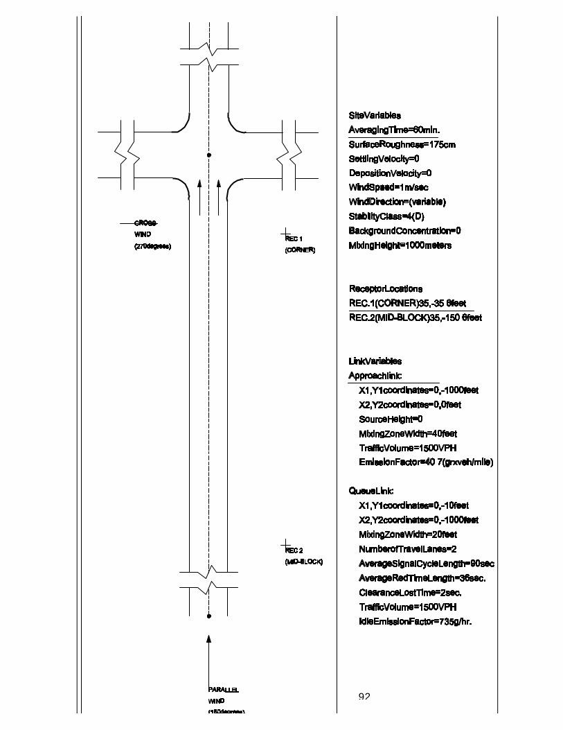
92

93

94
5.2 SIGNAL TIMING
Signal timing affects the computation in two ways. The emission source for the queue
links depends on both the idling emission factor and the fraction of red time (the larger
the fraction of red time, the stronger the emission source). In addition, the length of
the queue is determined by the volume to capacity ratio (V/C) of the approach link.
Since the capacity of the link is affected by the fraction of red time, the longer the red
phase, the smaller the available capacity, and the longer the queue length.
Three cases were analyzed: 30 percent red time, 40 percent red time, and 50 percent
red time. As seen in Figure 10, the increase in percent red time results in an increase of
CO. For the corner receptor the peak concentration, which occurs under a cross wind
condition in the case of 30 percent red (low V/C and short queues), shifts toward an
almost parallel wind condition for the 50 percent red case (higher V/C and longer
queues). For the midblock receptor, the CO increase is substantial when the length of
the queue reaches the midblock location.
5.3 TRAFFIC VOLUME ON THE QUEUE LINK
An increase in the traffic volume on an approach link will result in a longer queue
length but will not effect the strength of the emission source for the queue link. As
explained in Section 3.3.2, the strength of this line source is not dependent on the
approach volume. Three approach volumes were evaluated: 1000, 1500, and 2000
vehicles per hour (VPH). As seen in Figure 11, an increase in traffic volume results in
increased CO concentrations and a shift in peak CO values from a cross wind situation,
in the case of short queues, to a parallel wind condition, as the queues get longer. For
the midblock receptor, the CO increase is substantial when the length of the queue
reaches the midblock location.

95
Figure 10a. Variation of CO concentrations (ppm) at receptor 1 (corner) versus
wind angle for three different values of signal timing: 30% red time (V/C = 0.75, queue = 5.6 vehicles), 40% red time (V/C = 0.88, queue = 9.0 vehicles), and 50% red time (V/C = 1.08, queue = 42.9 vehicles).

96
Figure 10b. Same as Figure 10a except at receptor 2 (midblock)

97
Figure 11a. Variation of CO concentrations (ppm) at receptor 1 (corner) versus
wind angle for three different values of approach traffic volume: 1000 vph (V/C = 0.59, queue = 5.0 vehicles), 1500 vph (V/C = 0.88, queue = 9.0 vehicles), and 2000 vph (V/C = 1.18, queue = 93.5 vehicles).

98
Figure 11b. Same as Figure 11a except at receptor 2 (mid-block).

99
5.4 TRAFFIC LANES IN THE QUEUE LINK
The number of moving lanes affects the computations in two ways. First, the strength
of the emission source for a queue link is directly proportional to the number of moving
lanes (e.g. doubling the number of lanes at an intersection will double the source
strength). Second, the addition of lanes increases capacity. Thus by adding more
available lanes with the roadway traffic volume held constant, the length of the queue
is shortened. The net effect of these two components on CO concentrations is
dependent on the wind angle and the relative location of the receptor with respect to
the intersection. An increase of the number of available traffic lanes will not
necessarily result in a reduction of predicted CO concentration, since the strength of
the line source will increase (more rows of idling vehicles), but the queue will shorten
(less vehicles queuing per lane). If the receptor is very close to the intersection, with a
larger number of lanes under cross-wind conditions, higher CO levels may be predicted;
but if the receptor is further away from the intersection, a smaller number of lanes (a
longer queue) under near parallel winds will result in higher predicted CO levels. Two
cases were analyzed for two and three traffic lanes for the approach. As seen in Figure
12, even though the case with three traffic lanes has more capacity and shorter queues
compared with that of two traffic lanes, the cross wind condition results in higher CO
concentration at the corner receptor in the case of three traffic lanes. For the midblock
receptor, which is farther away from the intersection, two traffic lanes (with the longer
queues) result in higher CO concentrations.
5.5 TRAFFIC PARAMETERS
The three traffic parameters (Saturation Flow Rate, Signal Type, and Arrival Type)
affect the calculation of intersection capacity, delay, and queue length.

100
Figure 12a. Variation of CO concentrations (ppm) at receptor 1 (corner) versus
wind angle for different number of traffic lanes: two traffic lanes (V/C = 0.88, queue = 9.0 vehicles) and three traffic lanes (V/C = 0.59, queue = 5.0 vehicles).

101
Figure 12b. Same as Figure 12a except at receptor 2 (mid-block).

102
Saturation flow rate is used in the calculation of intersection capacity and V/C ratio,
having a direct effect of the calculation of approach delay; the lower the saturation
flow rate, the higher the delay. Signal type and arrival type are used in the calculation
of the progression adjustment factor which has an effect on the approach delay but
not on the V/C ratio; the worst the progression, the higher the approach delay.
The effect of these parameters on the resulting CO concentrations is only significant
when the intersection operates at medium to high V/C ratios (near or over saturation
conditions), which are the conditions when higher delay results in longer queues and
higher CO levels. In the case of light traffic conditions (low V/C ratios), the change in
approach delay has minimum effect on the length of the queue and the resulting CO
levels.

103
SECTION 6
MODEL VALIDATION
6.1 OVERVIEW
The U.S. EPA completed the performance evaluation of eight intersection models in
simulating CO concentrations at the six intersections monitored as part of the Route
9A Reconstruction Project in New York City2. The eight models evaluated included
CAL3QHC Version 2.0, FHWAINT14, GIM15, EPAINT14, CALINE416, VOL9MOB4 (Volume
94 updated with MOBILE4), TEXIN217, and IMM18. A complete phase I model
evaluation study was conducted using MOBILE4 emissions estimates. The phase I
evaluation included all eight intersection models at all six intersections. In late 1991,
the MOBILE4.1 emissions model9, an update to MOBILE4, was released. Thus, a phase
II evaluation utilizing MOBILE4.1 was conducted using a subset of the intersection
models. Of the three EPA intersection models (EPAINT, VOL9MOB4, and CAL3QHC),
CAL3QHC performed best using MOBILE4. Of the two models utilizing the FHWA
advocated average speed approach rather than explicit queuing (FHWAINT and GIM),
GIM performed best. Therefore, the phase II MOBILE4.1 analysis was performed for the
following five models: CAL3QHC, GIM, IMM, TEXIN2, and CALINE4. When collecting
and compiling the New York City database, the best quality assurance procedures (e.g.,
analysis and comparison of collected data) were followed at two of the six intersection
sites, Site #1 (West/Chambers) and Site #2 (34th/8th). A uniform wind analysis (e.g.,
similar wind speed and direction for different monitors at the same intersection)
conducted for each site indicated that Sites #5 (34th/12th) and #1 are best in terms of
unhindered approach wind flows and wind field uniformity. Thus, the phase II
MOBILE4.1 analysis was performed for the intersections at Sites #1, 2, and 5.
6.2 THE NEW YORK CITY DATABASE
A major air quality monitoring study was conducted in 1989-1990 in response to the
proposed reconstruction of a portion of Route 9A in New York City. As part of the
monitoring project, meteorological and CO air quality data were collected at two
background sites (Battery Park and Post Office) and six different intersections (Site #1
West/Chambers; #2 34th/8th; #3 65th/Broadway; #4 57th/7th; #5 34th/12th; #6
Battery Tunnel). These sites are all located in midtown or lower Manhattan. The

104
meteorological data collected at each intersection included wind direction, wind speed,
temperature, and the fluctuation of the wind direction (sigma theta). These data were
measured at two towers per intersection except at site #2 where they were measured
at three towers. The meteorological measurements were taken at a height of 10 m ± 1
m.
In order to obtain detailed information concerning the traffic characteristics, a series of
video cameras were used to film the traffic at each site. Three months of continuous
traffic data were collected at each site producing approximately 13,000 hours of video
recordings. A limited number of videotaped hours from the Route 9A Study were
examined in order to obtain detailed information about the local traffic. The collected
traffic data were concurrent with the observed CO data. The examined traffic data are
comprised of the top 50 hours of CO concentrations observed for each of three months
at Sites #1 and 2 and the top 25 hours observed for each of three months at the
remaining sites.
All traffic data were obtained from videotapes except for the acceleration/deceleration
rates and the cruise speed. The acceleration/deceleration rates and cruise speeds were
obtained through the use of a vehicle outfitted with a travel-log machine that recorded
instantaneous speed versus time while traveling. Cruise speeds were taken directly
from the strip charts created in this way; acceleration/deceleration rates were
determined from the slope of the lines on the strip charts.
6.3 MODELING METHODOLOGY
The hourly averaged temperature data from the meteorological towers at each site were
averaged to calculate a site specific hourly value. For the remaining meteorological
input data, the meteorological tower closest to the CO monitor location was used.
Mixing heights of 1000 m were used, since the results are not affected if the mixing
height is between 100 and 1000 m high and mixing heights below 100 m in Manhattan
do not occur on a frequent basis.
The closest background concentration (Battery Park or the Post Office Station) was
subtracted out of the observed concentration at each monitor. All modeling was
performed for one hour averages only. After the removal of the background

105
concentrations, a screening threshold of 0.5 ppm was used. When both the observed
and predicted concentrations at a monitor are less than 0.5 ppm that data pair was
eliminated from the data set.
A surface roughness length of 3.21 m was used for approach flows over numerous city
blocks. Lower values of the surface roughness length (0.03 m) were used at Site #5
(34th/12th) when the intersection was exposed to flows over the Hudson River without
intervening buildings. For modeling CO concentrations, the settling velocity and
deposition velocity were set at zero because CO is a gaseous emission. An averaging
time of 60 minutes was used. Finally, a temperature-sensitive conversion of the
modeled concentrations from mg/m3 to parts per million (ppm) was conducted.
6.4 MODEL EVALUATION RESULTS
6.4.1 Regulatory Default Analysis
The ten hours with the highest observed concentrations were used to compare the
CAL3QHC predicted concentrations using the regulatory default meteorology to the
observed concentrations. The comparisons for each site are presented in Table 6. The
regulatory default meteorological conditions are defined as: Wind Speed = 1 m/s; Stability Class = D; Sigma-Theta = 25°; Observed Temperature; and "Worst Case"
Wind Direction Angle (determined using ten degree increments).
At Site #1, the highest observed CO concentration of 10.6 ppm is nearly matched
(10.4 ppm) by CAL3QHC unpaired in time or space. At Site #2, the maximum
predicted concentration by CAL3QHC of 8.0 ppm underpredicts the maximum observed
concentration of 11.5 ppm. Finally, at Site #5, the maximum observed concentration
of 15.5 ppm is nearly matched by CAL3QHC which predicts 15.1 ppm.
6.4.2 Scoring Scheme Results
A method for aggregating component results of model performance (using the
observed meteorology) into a single performance measure19 was used to compare the
overall performance of the five models evaluated at three intersection sites. The
bootstrap

106
TABLE 6
COMPARISON OF TOP TEN OBSERVED CONCENTRATIONS WITH
CAL3QHC PREDICTED CONCENTRATIONS
Site #1 Site #2 Site #5
Observed Predicted Observed Predicted Observed Predicted
ppm ppm ppm ppm ppm ppm
10.6 7.5 11.5 5.4 15.5 9.2
9.1 9.8 10.5 8.0 14.6 8.4
9.0 9.8 10.4 7.0 10.4 11.5
8.6 7.0 10.2 6.9 9.9 10.3
8.2 10.4 10.2 3.9 9.3 11.4
7.8 8.2 9.1 4.7 8.9 10.5
7.6 10.0 8.8 4.9 8.7 10.7
7.5 9.8 8.5 7.3 8.4 11.6
7.5 8.0 8.4 6.7 7.6 15.1
7.4 9.9 8.3 6.1 7.4 10.8

107
re-sampling technique20 was used to determine the significance of differences in composite
performance between models.
The statistical analysis uses the robust highest concentration (RHC) for one-hour averages.
The RHC is based on a tail exponential fit to the upper end of the distribution and is
calculated as follows
where
Install Equa tion Editor and double -click here to view equation. 1 = average of the n-1 largest values
x(n) = nth largest value
n = number of values exceeding the threshold value (n=26 or less)
The size of the three intersection data sets requires the value of n to be less than 26. The
value of n was nominally set to 11 so that the number of values averaged
(
Install Equa tion Editor and double -click here to view equation. 2) was 10. In general, the RHCs are largest using the
operational (or entire) dataset for each site. When calculating either the fractional bias (FB) or the absolute fractional bias (AFB),
where OB and PR refer to the averages of the observed and predicted values, the RHC is
used rather than the mean of the highest 10 concentrations. The RHC is preferred in this
type of statistical evaluation because of its stability19. Also, the bootstrap distribution of
the RHCs is not artificially bounded at the maximum predicted or observed concentration,
which allows for a continuous range of concentrations.
When comparing these performance measures, one would like to know if differences are
significant. Simultaneous confidence intervals for each pair of models were calculated21 in
order to ensure an adequate confidence level and to protect against falsely concluding that
two models are different. A composite performance measure (CPM) is calculated for each
model as a weighted linear combination of the individual absolute fractional bias
components. The operational component is given a weight that is equal to the weight of
the combined scientific components. The scientific component refers to the evaluation of
peak concentrations during specific meteorological conditions and the operational
Install Equa tion Editor and double -click here to view equation. (5)
Install Equa tion Editor and double -click here to view equation. (6)

108
component refers to the evaluation of peak averages independent of meteorological
conditions. The results from the different data bases (intersections) are given equal
weight. The CPM is defined as
where AFB(i)= Absolute fractional bias weighted for each scientific category i,
AFB(1)= Absolute fractional bias for the operational one-hour averages.
The wind speed (u) ≤ 6 mph and neutral/stable category is weighted more than the other
two categories because of the importance of this category for regulatory modeling
purposes. Thus, the average of AFB(i) is
A combination of the CPM values across all three sites yields the composite model
comparison measure (CM). The CM results, shown in Figure 13, indicates that the best
performing models are CAL3QHC, TEXIN2, and CALINE4. Similarly, the AFB from scientific category 1 (u ≤ 6 mph, neutral/stable) can also be combined over all three sites into a single
model comparison measure (CM). This category is typically most important in terms of
regulatory applications. As shown in Figure 14, CAL3QHC has the lowest CM by a factor
of two.
Install Equa tion Editor and double -click here to view equation. (7)
Install Equa tion Editor and double -click here to view equation. (8)

109
Figure 13. The composite model comparison measure (CM) with 95% confidence limits using CPM statistics.

110

111
Figure 14. CM with 95% confidence limits using AFB of scientific category 1.

112

113
REFERENCES 1. Benson, P., CALINE-3 - A Versatile Dispersion Model for Predicting Air Pollutant
Levels Near Highways and Arterial Streets. Office of Transportation Laboratory, California DOT, Sacramento, California. FHWA/CA/TL-79/23, Nov. 1979.
2. U.S. Environmental Protection Agency, Evaluation of CO Intersection Modeling
Techniques Using a New York City Database. U.S. EPA, OAQPS, Research Triangle Park, North Carolina, EPA-454/R-92-004, 1992.
3. Transportation Research Board (TRB), The Highway Capacity Manual. TRB Special
Report 209. Washington, D.C., 1985. 4. U.S. Environmental Protection Agency, Guidelines for Air Quality Maintenance
Planning and Analysis, Volume 9 (Revised): Evaluating Indirect Sources. U.S. EPA Office of Air, Noise and Radiation, Research Triangle Park, North Carolina. EPA-450/4-78-001- OAQPS No.1.2-028R, 1979.
5. Newell G.F., Applications of Queuing Theory. 2nd edition, 1982. 6. Akcelik Rahmi, The Highway Capacity Manual Delay Formula for Signalized
Intersections. ITE Journal Volume 58 No 3, March 1988. 7. Webster F.B. and Cobee B.M., Traffic Signals - Road Research Technical Paper No 56.
Road Research Laboratory, 1966. 8. Webster F.B., Traffic and Signal Settings - Road Research Technical Paper No 39.
Road Research Laboratory 1958. 9. U.S. Environmental Protection Agency, User's Guide to MOBILE5 (Mobile Source
Emissions Factor Model). U.S. EPA, Ann Arbor, Michigan, EPA-AA-AQAB-94-01, 1994.
10. Randall, Patrick C. and Ng, Harry N.C., Air Quality Analysis Tools (AQAT-2). State of
California Air Resources Board, Technical Support Division, Sacramento, CA, 1987. 11. U.S. Environmental Protection Agency, User's Guide to PART5: A Program for
Calculating Particulate Emissions from Motor Vehicles. U.S. EPA, Ann Arbor, Michigan, EPA-AA-
AQAB-94-02, 1995. 12. Institute of Transportation Engineers, Transportation and Traffic Engineering
Handbook. 2nd edition, 1982.

114
13. Wallace, C.E. et al, TRANSYT 7FF Traffic Network Study Tool Version 7F) - User's Manual. University of Florida Transportation Research Center & Federal Highway Administration, 1984.
14. PEI, Development and Review of Traffic and CO Emission Components of Intersection
Modeling Techniques. U.S. EPA, Research Triangle Park, NC, 1988. 15. EMI Consultants, The Georgia Intersection Model for Air Quality Analysis. Knoxville,
TN, 1985. 16. Benson, P., CALINE4 - A Dispersion Model for Predicting Air Pollutant Concentrations
Near Roadways. Report No. FHWA/CA/TL-84/14. Office of Transportation Laboratory, Sacramento, CA, 1989.
17. Bullin, G., J. Korpics, and M. Hlavinka, User's Guide to the TEXIN2/MOBILE4 Model.
Research Report 283-2. Texas State Department of Highways and Public Transportation, College Station, TX, 1990.
18. NYDOT, Intersection Midblock Model User's Guide. New York State Department of
Transportation, Albany, NY, 1982. 19. Cox, W.M. and J.A. Tikvart, A Statistical Procedure for Determining the Best
Performing Air Quality Simulation Model. Atm. Env., 24, 2387-2395, 1990. 20. Efron, B., The Jackknife, the Bootstrap and Other Resampling Plans. Society for
Industrial and Applied Mathematics, Philadelphia, PA, 1982. 21. Cleveland, W.S. and R. McGill, Graphical Perception: Theory, Experimentation, and
Application to the Development of Graphical Methods. J. Am. Stat. Assoc., 79, 531-554, 1984.

115