EOE 2204 1

EOE 2204RESEARCH METHODS IN

ENVIRONMENTAL SCIENCE

Prof Paul WorsfoldPortland Square Development B520Email pworsfold@plymouth.ac.uk

(But not too often!)

Contents stored on sharepoint

EOE 2204 2

Introduction to Environmental Analytical Chemistry

This presentation is intended to provide support material for the Wembury field and lab work. Any of the material in steps 1-5 could be included in an exam question.

The six steps in the “Analytical Approach” to any problem are:

1. Defining the problem

2. Sampling (Waters and Sediments)

3. Sample Treatment (Digestion of sediments, preservation of waters)

4. Measurement

5. Data Treatment (Precision, Accuracy, Calibration, Limit of Detection)

6. Report Writing

EOE 2204 3

Analytical Chemistry Definition

The science which deals with the detection, identification and quantification of chemical species in matrices of chemical, biological or environmental origin. It is a multidisciplinary subject that has chemistry at its core but also requires a knowledge of other sciences, e.g. biology, biochemistry, physics, mathematics, statistics and computing. It is concerned with the real world, with the primary aim of determining WHAT constituents (qualitative analysis) are present in a sample and HOW MUCH of each constituent (quantitative analysis) is present.

EOE 2204 4

Environmental Analytical Chemistry

Common matrices/Application areas include;

• Hydrosphere•e.g. sea, river, estuary, lake, porewater

• Atmosphere•e.g. outdoor air, workplace air, air-sea interface

• Lithosphere•e.g. soil, sediment. rocks

• Biosphere•e.g. plants, animals, humans

EOE 2204 5

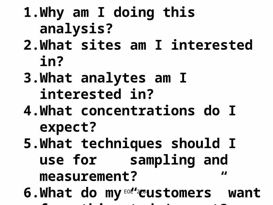
1. DEFINING THE PROBLEM

1. Why am I doing this analysis?2. What sites am I interested in?3. What analytes am I interested in?4. What concentrations do I expect?5. What techniques should I use for

sampling and measurement?6. What do my “customers” want

from this study/report?

EOE 2204 6

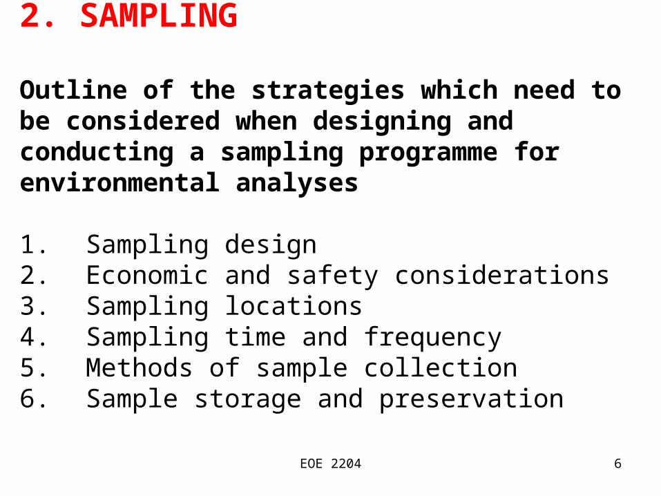
2. SAMPLING

Outline of the strategies which need to be considered when designing and conducting a sampling programme for environmental analyses

1. Sampling design2. Economic and safety considerations3. Sampling locations4. Sampling time and frequency5. Methods of sample collection6. Sample storage and preservation

EOE 2204 7

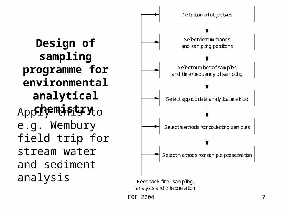
Feedback from sampling,analysis and interpretation

Select methods for sample preservation

Select methods for collecting samples

Select appropriate analytical method

Select number of samplesand time/frequency of sampling

Select determinandsand sampling positions

Definition of objectives

Design of sampling programme for environmental

analytical chemistry

Apply this to e.g. Wembury field trip for stream water and sediment analysis

EOE 2204 8

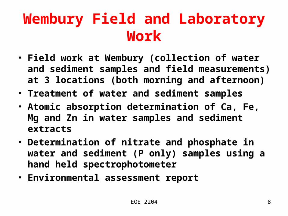
Wembury Field and Laboratory Work

• Field work at Wembury (collection of water and sediment samples and field measurements) at 3 locations (both morning and afternoon)

• Treatment of water and sediment samples • Atomic absorption determination of Ca, Fe, Mg and

Zn in water samples and sediment extracts• Determination of nitrate and phosphate in water and

sediment (P only) samples using a hand held spectrophotometer

• Environmental assessment report

EOE 2204 9

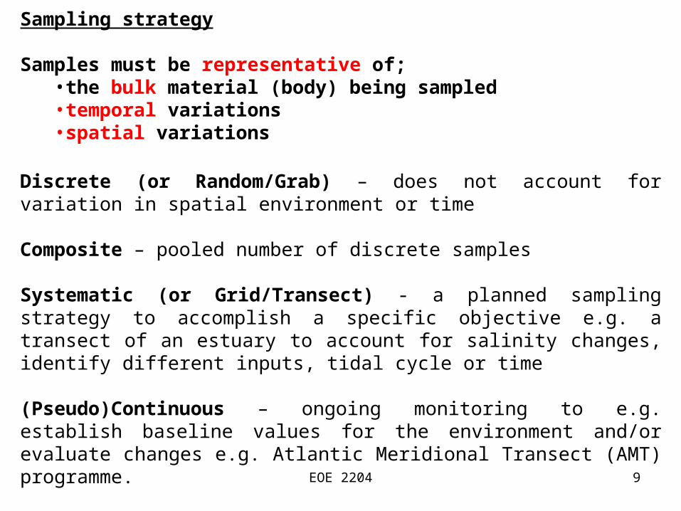
Sampling strategy

Samples must be representative of;•the bulk material (body) being sampled•temporal variations•spatial variations

Discrete (or Random/Grab) – does not account for variation in spatial environment or time

Composite – pooled number of discrete samples

Systematic (or Grid/Transect) - a planned sampling strategy to accomplish a specific objective e.g. a transect of an estuary to account for salinity changes, identify different inputs, tidal cycle or time

(Pseudo)Continuous – ongoing monitoring to e.g. establish baseline values for the environment and/or evaluate changes e.g. Atlantic Meridional Transect (AMT) programme.

EOE 2204 10

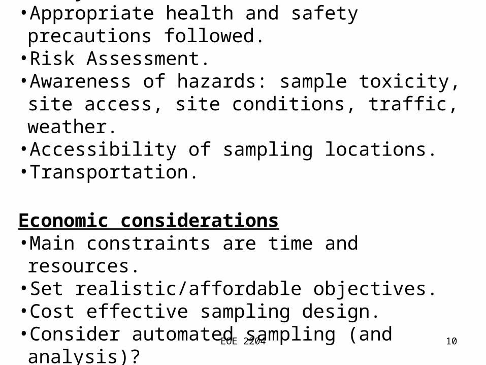
Safety Considerations• Appropriate health and safety precautions followed.• Risk Assessment.• Awareness of hazards: sample toxicity, site access, site conditions, traffic, weather.

• Accessibility of sampling locations.• Transportation.

Economic considerations• Main constraints are time and resources.• Set realistic/affordable objectives.• Cost effective sampling design.• Consider automated sampling (and analysis)?

EOE 2204 11

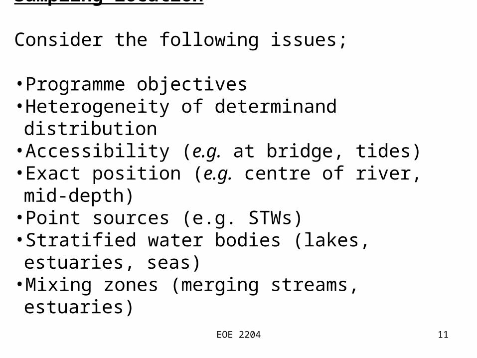
Sampling location

Consider the following issues;

• Programme objectives• Heterogeneity of determinand distribution• Accessibility (e.g. at bridge, tides)• Exact position (e.g. centre of river, mid-depth)• Point sources (e.g. STWs)• Stratified water bodies (lakes, estuaries, seas)• Mixing zones (merging streams, estuaries)

EOE 2204 12

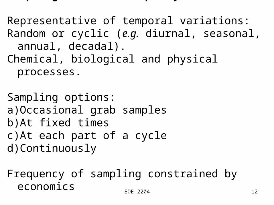
Sampling Time and Frequency

Representative of temporal variations:Random or cyclic (e.g. diurnal, seasonal, annual,

decadal).Chemical, biological and physical processes.

Sampling options: a)Occasional grab samplesb)At fixed timesc)At each part of a cycled)Continuously

Frequency of sampling constrained by economics

EOE 2204 13

Methods of Sample CollectionSampling devices:Water: Submersible pumps, Glass or plastic (polyethylene) bottles, Depth sampling bottles.Sediment and soils:, Scoops and trowels, Corers and dredgers

Need to avoidContamination from sampling device and storage container. Glass – Use for organics. Ion exchange sites can remove metal ions from solution. Plasticware e.g. HDPE – Use for inorganics. Possible leaching of organics from container.

EOE 2204 14

Sample bottlesGlass – is used for organic analysis. Easily cleaned but cant be frozen.Plasticware - e.g. high density polyethylene (HDPE) is used for nutrients and trace metals. Can be frozen.

Cleaning protocols – should be defined in the sampling strategy from the outset and can differ depending on the analyte under investigation and containers used.

Cleaning protocols - trace level analysis Pre-washing by soaking in hot detergent for 24 hcopious rinsing with pure water and then ultra high purity water (UHP) 5 days in an acid bath (HCl)copious (3x) rinsing with UHP 5 days in an acid bath (HNO3)

copious (3x) rinsing with UHP

EOE 2204 15

3. SAMPLE TREATMENT (WATERS)

Sample Preservation and StorageThe aim is to minimise potential changes to the sample during storage. Processes that can affect sample integrity include:

•Biodegradation (e.g. N and P compounds)•Oxidation (e.g. Fe(II), organic compounds)•Absorption of CO2 (e.g. pH, alkalinity)•Precipitation (e.g. CaCO3, Al(OH)3)•Volatilisation (e.g. O2, HCN)•Adsorption (e.g. dissolved metals)

EOE 2204 16

Changes can be retarded (not prevented) by

Refrigeration (reduces biological activity)

Freezing (plastic bottles only)

Filtration (removes biotic and abiotic particulate matter but not all bacteria and viruses)

Preserving agents: Concentrated; added during sampling, Acidification (e.g. HCl) for trace metals, Biocides (e.g. HgCl2) for biodegradable determinands

EOE 2204 17

Filtration

• Separation of dissolved and particulate determinands (0.45 m membrane filter) is operationally defined

• Can use other sizes, e.g. 0.2 m

• Perform immediately

• Filters should be pre-washed

• Removes most biotic and abiotic particles but not all bacteria, viruses and colloids

EOE 2204 18

3. SAMPLE TREATMENT (SEDIMENTS)

A sample size of ~ 0.1 – 5 g is usually enough for analysis. This is obtained by dividing up the originally collected sample.

The less than 180 um size fraction of inorganic material is often used and may require grinding. This helps provide a more homogeneous sample and assists the dissolution (digestion) process.

“Coning and quartering” - the reduction of the bulk sample to a suitable sample size for analysis whereby the sample is dumped to form a cone, which is then flattened. The circular layer is divided into four equal segments and two opposite quarters are discarded. The operation is repeated with the remainder until the required amount is left.

EOE 2204 19

Methods of Sample Digestion

Wet digestion (ashing) in an open vessel (flask) is the most common approach for elemental analysis. Various acids can be used, e.g. a mixture of nitric (oxidising) and hydrochloric (reducing) acids which is known as aqua regia or nitric acid alone. To speed up the process a closed pressurised vessel (e.g. PTFE bomb) and/or a microwave can be used.

Dry ashing involves heating the sample in an open platinum or glazed porcelain crucible at 450 - 550 oC in a muffle furnace until the residue is white or nearly so. It is then extracted with hot hydrochloric acid.

EOE 2204 20

Properties of commonly used acids for digestion of soils and sediments

NITRIC acid (70%) is acidic and oxidising and forms soluble salts (except oxides of Al, Nb, Ta, Ti, Sn, Sb, W). Used alone or with bromine or hydrochloric acid.

HYDROCHLORIC acid (36%) is acidic and non-oxidising (reducing for some higher oxidation states) and chlorides are generally soluble (except Ag, Hg, Tl, Pb). Some chlorides volatile (Hg, Ge, As, Sb, Se). Widely used for inorganic matrices but not for organic matrices. Used alone or plus either (1) a reducing agent such as tin(II) chloride or hyrazine hydrochloride, or (2) an oxidising agent such as bromine, nitric acid, perchloric acid.

EOE 2204 21

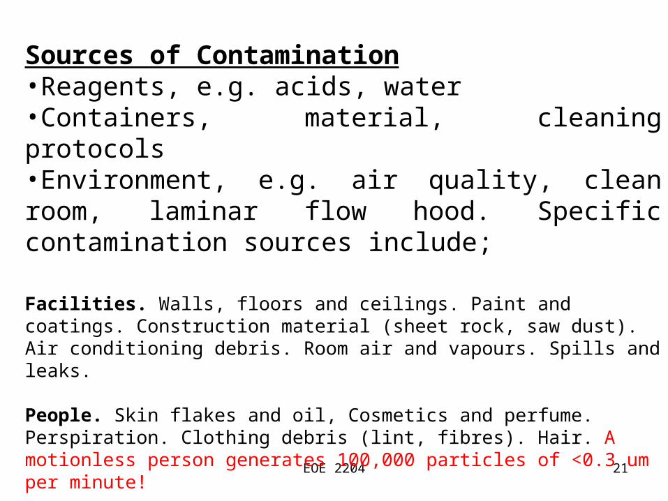
Sources of Contamination•Reagents, e.g. acids, water•Containers, material, cleaning protocols•Environment, e.g. air quality, clean room, laminar flow hood. Specific contamination sources include;

Facilities. Walls, floors and ceilings. Paint and coatings. Construction material (sheet rock, saw dust). Air conditioning debris. Room air and vapours. Spills and leaks.

People. Skin flakes and oil, Cosmetics and perfume. Perspiration. Clothing debris (lint, fibres). Hair. A motionless person generates 100,000 particles of <0.3 um per minute!

Fluids. Particulates floating in air (dust). Bacteria, organics and moisture. Floor finishes or coatings. Cleaning chemicals. Plasticizers (outgasses). Deionized water.

EOE 2204 22

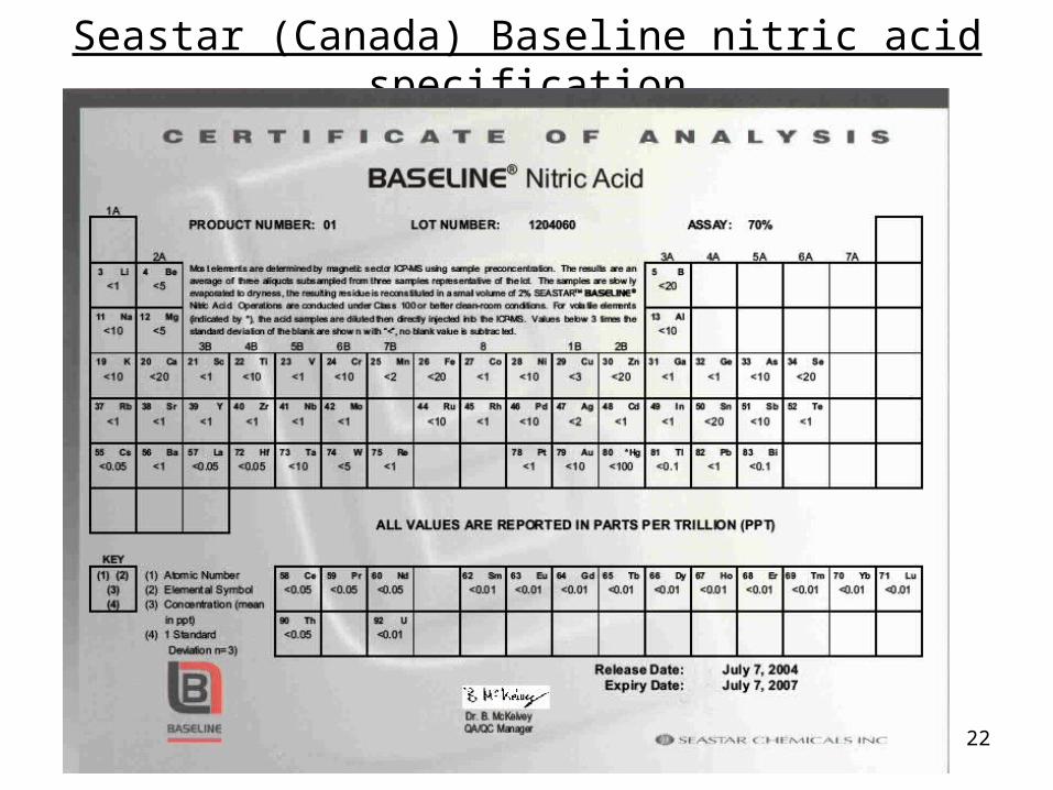
Seastar (Canada) Baseline nitric acid specification

EOE 2204 23

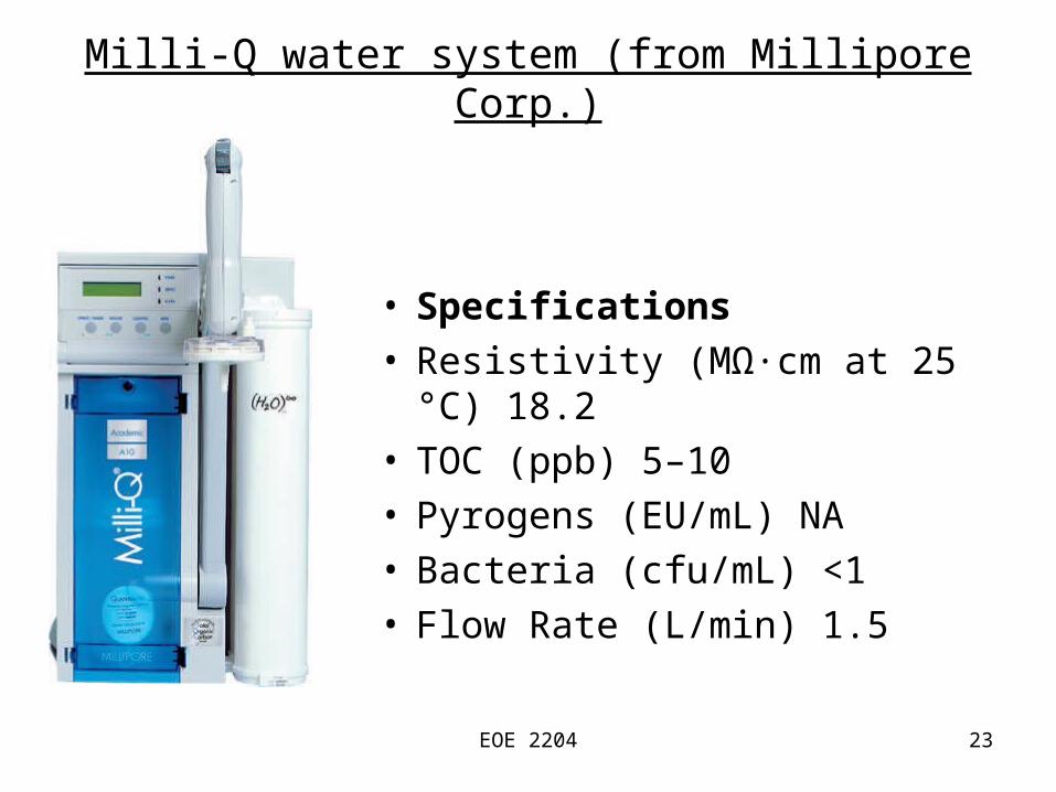
Milli-Q water system (from Millipore Corp.)

• Specifications• Resistivity (MΩ·cm at 25 °C) 18.2 • TOC (ppb) 5–10• Pyrogens (EU/mL) NA• Bacteria (cfu/mL) <1• Flow Rate (L/min) 1.5 

EOE 2204 24

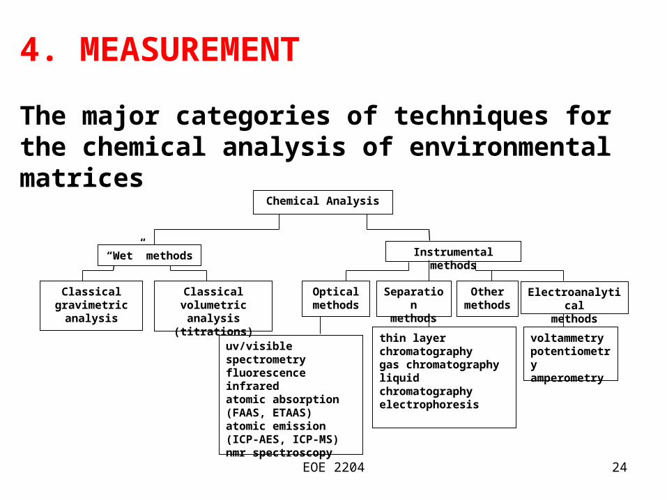
Chemical Analysis

“Wet” methods Instrumental methods

Classicalgravimetric

analysis

Classicalvolumetric analysis

(titrations)

Opticalmethods

Separationmethods

Othermethods

Electroanalyticalmethods

uv/visible spectrometryfluorescenceinfraredatomic absorption (FAAS, ETAAS)atomic emission (ICP-AES, ICP-MS)nmr spectroscopy

thin layer chromatographygas chromatographyliquid chromatographyelectrophoresis

voltammetrypotentiometryamperometry

4. MEASUREMENT

The major categories of techniques for the chemical analysis of environmental matrices

EOE 2204 25

5. DATA TREATMENT

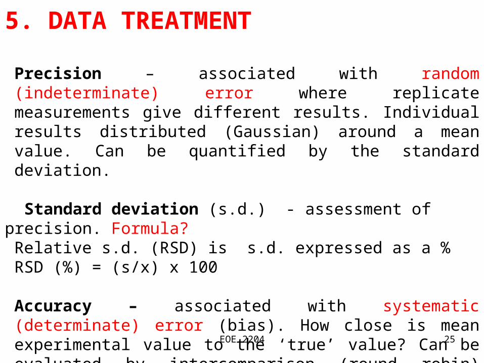
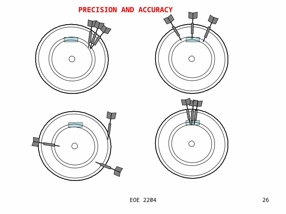
Precision – associated with random (indeterminate) error where replicate measurements give different results. Individual results distributed (Gaussian) around a mean value. Can be quantified by the standard deviation.

Standard deviation (s.d.) - assessment of precision. Formula?Relative s.d. (RSD) is s.d. expressed as a %RSD (%) = (s/x) x 100

Accuracy – associated with systematic (determinate) error (bias). How close is mean experimental value to the ‘true’ value? Can be evaluated by intercomparison (round robin) exercises and use of certified reference materials (CRMs).

EOE 2204 26

PRECISION AND ACCURACY

EOE 2204 27

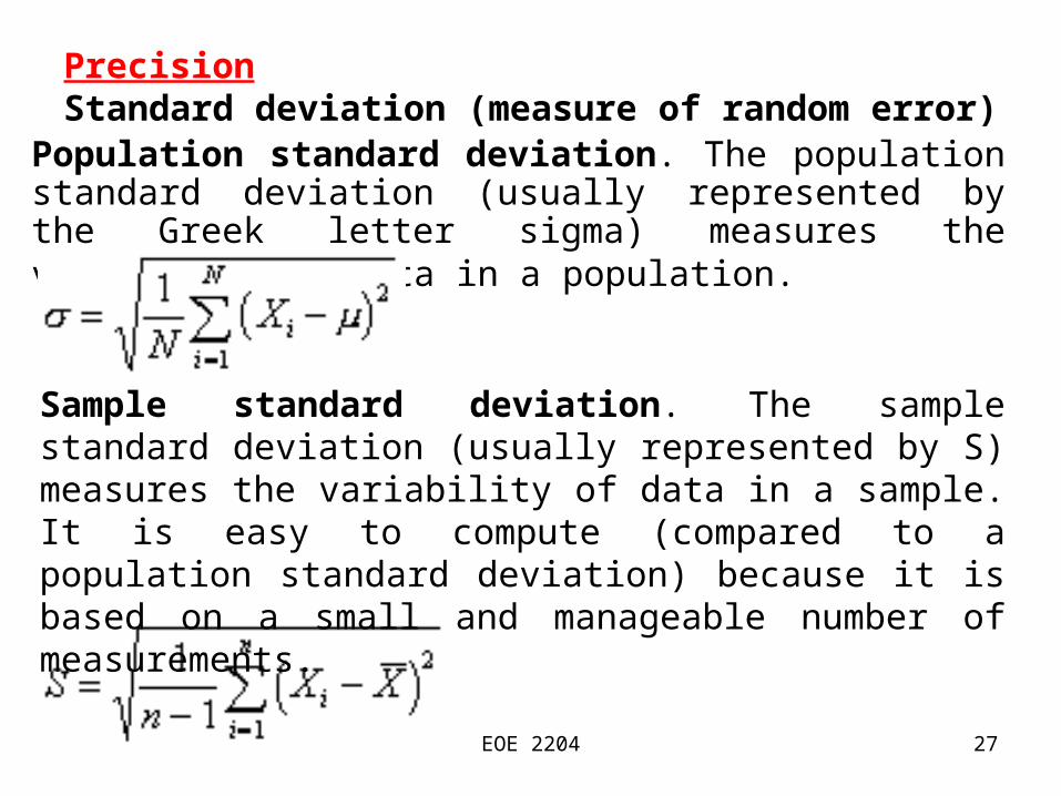
PrecisionStandard deviation (measure of random error)

Population standard deviation. The population standard deviation (usually represented by the Greek letter sigma) measures the variability of data in a population.

Sample standard deviation. The sample standard deviation (usually represented by S) measures the variability of data in a sample. It is easy to compute (compared to a population standard deviation) because it is based on a small and manageable number of measurements.

EOE 2204 28

The standard deviation assumes a Normal (Gaussian) distribution of data from replicate determinations (usually 4 or 5). It is symmetrical about the mean and the greater the value of s the greater the spread of the ‘bell shape’. +/- 1s - includes 68 % of sample population +/- 2s - includes 95 % of sample population+/- 3s - includes 99 % of sample population

Mean (x) = Arithmetic estimate of true value (μμ))

Spread or range = difference between largest and smallest measured value

Confidence intervals can be used to test for systematic errors – measure CRM, derive confidence interval and if known value is not within confidence interval then systematic error is probably present.

EOE 2204 29

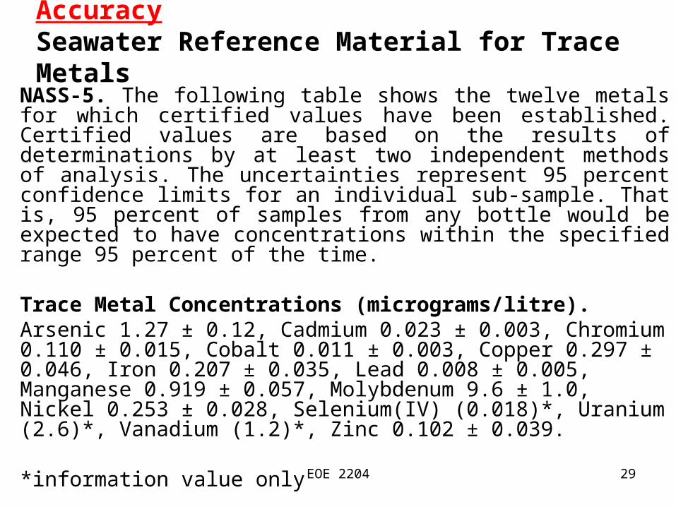
AccuracySeawater Reference Material for Trace Metals

NASS-5. The following table shows the twelve metals for which certified values have been established. Certified values are based on the results of determinations by at least two independent methods of analysis. The uncertainties represent 95 percent confidence limits for an individual sub-sample. That is, 95 percent of samples from any bottle would be expected to have concentrations within the specified range 95 percent of the time.

Trace Metal Concentrations (micrograms/litre).Arsenic 1.27 ± 0.12, Cadmium 0.023 ± 0.003, Chromium 0.110 ± 0.015, Cobalt 0.011 ± 0.003, Copper 0.297 ± 0.046, Iron 0.207 ± 0.035, Lead 0.008 ± 0.005, Manganese 0.919 ± 0.057, Molybdenum 9.6 ± 1.0, Nickel 0.253 ± 0.028, Selenium(IV) (0.018)*, Uranium (2.6)*, Vanadium (1.2)*, Zinc 0.102 ± 0.039.

*information value only

EOE 2204 30

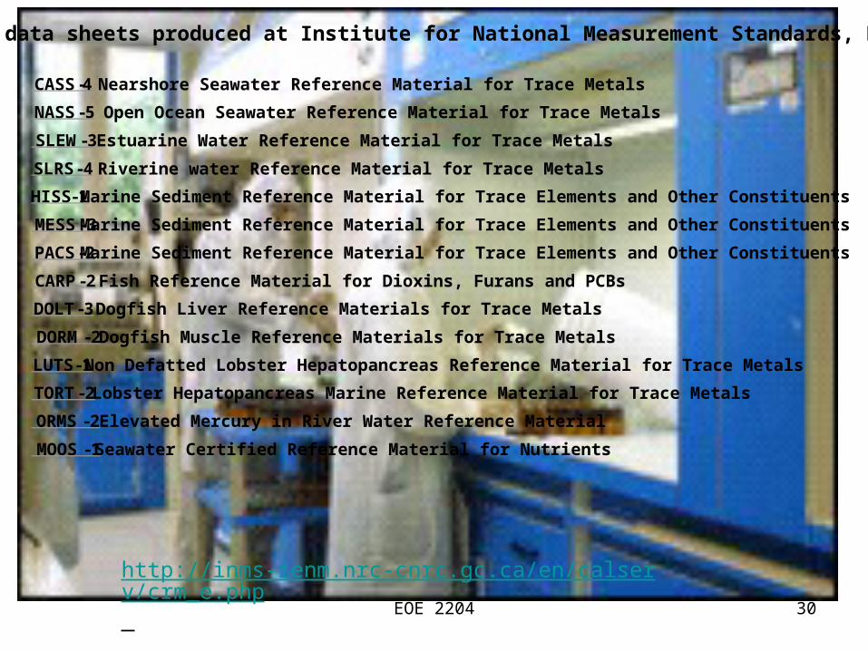
http://inms-ienm.nrc-cnrc.gc.ca/en/calserv/crm_e.php

CRM data sheets produced at Institute for National Measurement Standards, NRCC

CASS-4 Nearshore Seawater Reference Material for Trace Metals

NASS-5 Open Ocean Seawater Reference Material for Trace Metals

SLEW-3 Estuarine Water Reference Material for Trace Metals

SLRS-4 Riverine water Reference Material for Trace Metals

HISS-1 Marine Sediment Reference Material for Trace Elements and Other Constituents

MESS-3 Marine Sediment Reference Material for Trace Elements and Other Constituents

PACS-2 Marine Sediment Reference Material for Trace Elements and Other Constituents

CARP-2 Fish Reference Material for Dioxins, Furans and PCBs

DOLT-3 Dogfish Liver Reference Materials for Trace Metals

DORM -2 Dogfish Muscle Reference Materials for Trace Metals

LUTS-1 Non Defatted Lobster Hepatopancreas Reference Material for Trace Metals

TORT-2 Lobster Hepatopancreas Marine Reference Material for Trace Metals

ORMS-2 Elevated Mercury in River Water Reference Material

MOOS -1 Seawater Certified Reference Material for Nutrients

EOE 2204 31

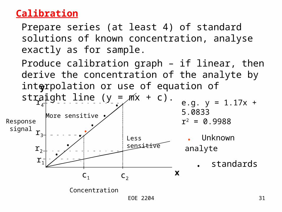
Calibration

Prepare series (at least 4) of standard solutions of known concentration, analyse exactly as for sample.

Produce calibration graph – if linear, then derive the concentration of the analyte by interpolation or use of equation of straight line (y = mx + c).

Responsesignal

Concentration

y

r4

c1 c2

r1

r3

r2

More sensitive

Less sensitive

x

..

..

..

.

e.g. y = 1.17x + 5.0833r2 = 0.9988

. Unknown analyte

. standards

EOE 2204 32

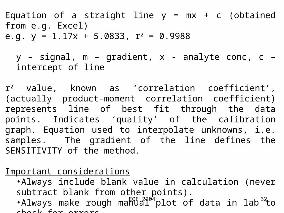
Equation of a straight line y = mx + c (obtained from e.g. Excel)e.g. y = 1.17x + 5.0833, r2 = 0.9988

y – signal, m – gradient, x - analyte conc, c – intercept of line

r2 value, known as ‘correlation coefficient’, (actually product-moment correlation coefficient) represents line of best fit through the data points. Indicates ‘quality’ of the calibration graph. Equation used to interpolate unknowns, i.e. samples. The gradient of the line defines the SENSITIVITY of the method.

Important considerations•Always include blank value in calculation (never subtract blank from other points). •Always make rough manual plot of data in lab to check for errors.•Is response linear? For analytical data need at least 0.99.•What is the best straight line (slope and intercept) through the data points?

EOE 2204 33

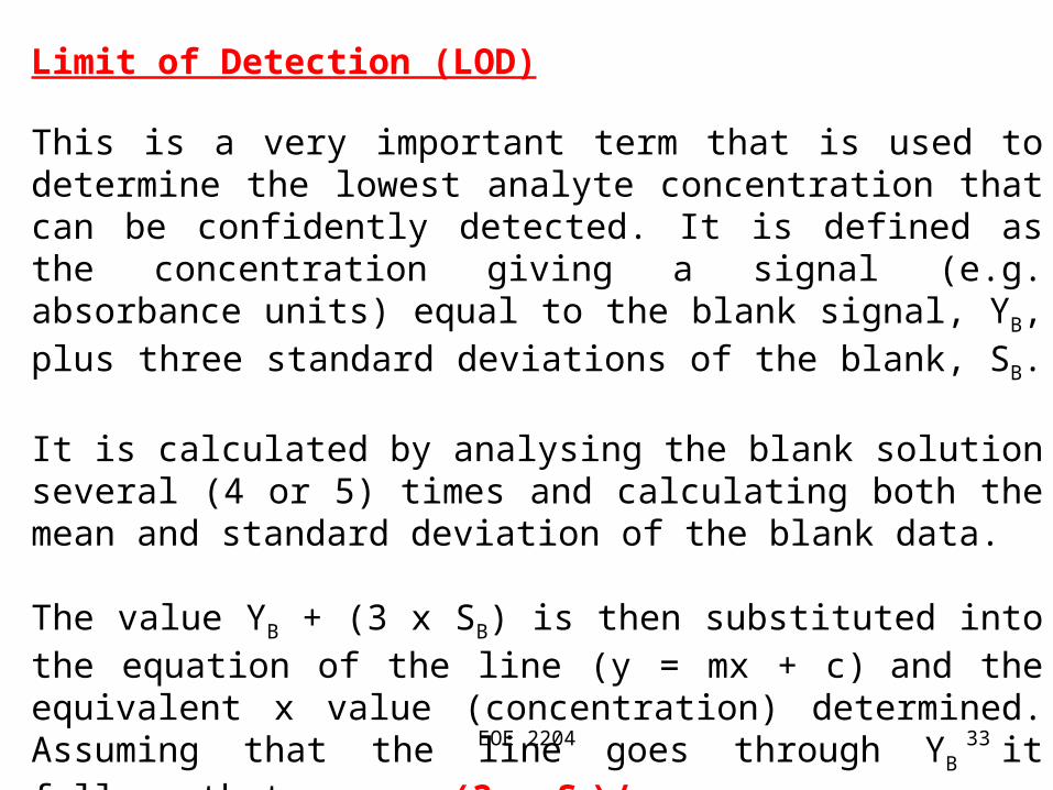
Limit of Detection (LOD)

This is a very important term that is used to determine the lowest analyte concentration that can be confidently detected. It is defined as the concentration giving a signal (e.g. absorbance units) equal to the blank signal, YB, plus three standard deviations of the blank, SB.

It is calculated by analysing the blank solution several (4 or 5) times and calculating both the mean and standard deviation of the blank data.

The value YB + (3 x SB) is then substituted into the equation of the line (y = mx + c) and the equivalent x value (concentration) determined. Assuming that the line goes through YB it follows that x(LOD) = (3 x SB)/m.

EOE 2204 34

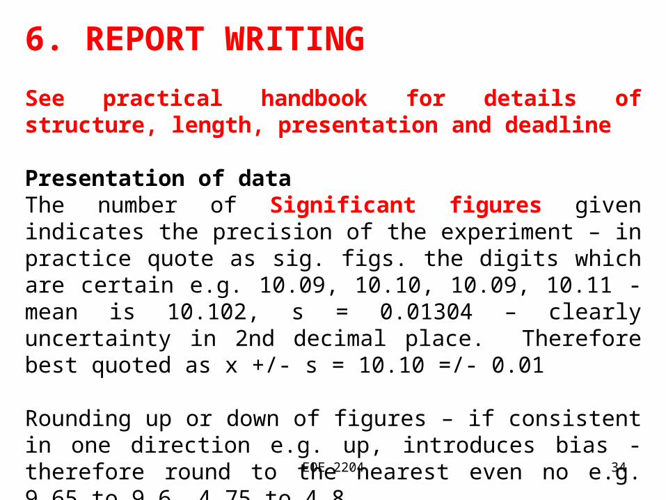
6. REPORT WRITING

See practical handbook for details of structure, length, presentation and deadline

Presentation of dataThe number of Significant figures given indicates the precision of the experiment – in practice quote as sig. figs. the digits which are certain e.g. 10.09, 10.10, 10.09, 10.11 - mean is 10.102, s = 0.01304 – clearly uncertainty in 2nd decimal place. Therefore best quoted as x +/- s = 10.10 =/- 0.01

Rounding up or down of figures – if consistent in one direction e.g. up, introduces bias - therefore round to the nearest even no e.g. 9.65 to 9.6, 4.75 to 4.8

EOE 2204 35

EOE 2204 36

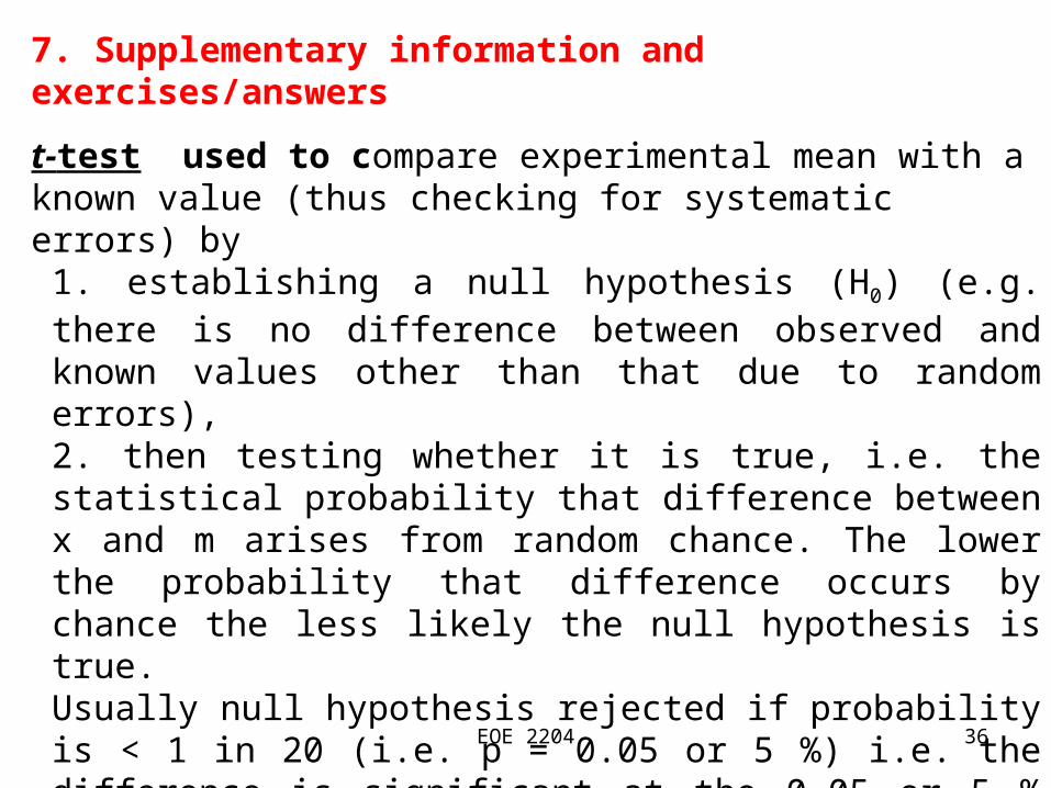
7. Supplementary information and exercises/answers

t-test used to compare experimental mean with a known value (thus checking for systematic errors) by

1. establishing a null hypothesis (H0) (e.g. there is no difference between observed and known values other than that due to random errors), 2. then testing whether it is true, i.e. the statistical probability that difference between x and m arises from random chance. The lower the probability that difference occurs by chance the less likely the null hypothesis is true. Usually null hypothesis rejected if probability is < 1 in 20 (i.e. p = 0.05 or 5 %) i.e. the difference is significant at the 0.05 or 5 % level. Increased certainty by using p = 0.01 or 0.001 (1 % or 0.1 %) 3. The value of the t is calculated, if this is less than a critical value (taken from tables) then the null hypothesis is accepted.

EOE 2204 37

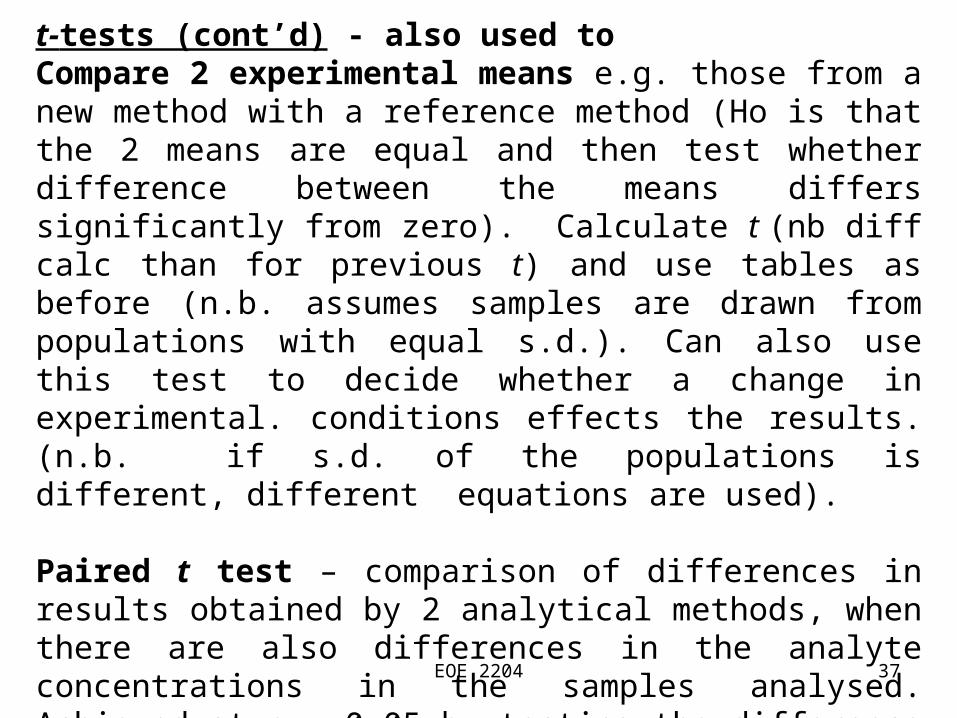
t-tests (cont’d) - also used toCompare 2 experimental means e.g. those from a new method with a reference method (Ho is that the 2 means are equal and then test whether difference between the means differs significantly from zero). Calculate t (nb diff calc than for previous t) and use tables as before (n.b. assumes samples are drawn from populations with equal s.d.). Can also use this test to decide whether a change in experimental. conditions effects the results. (n.b. if s.d. of the populations is different, different equations are used).

Paired t test – comparison of differences in results obtained by 2 analytical methods, when there are also differences in the analyte concentrations in the samples analysed. Achieved at p = 0.05 by testing the difference (d) between each pair of results - Ho = d does not differ significantly from 0

EOE 2204 38

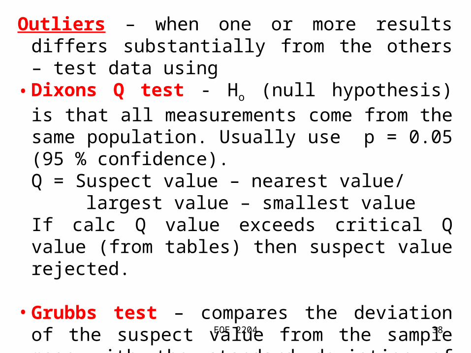
Outliers – when one or more results differs substantially from the others – test data using

• Dixons Q test - Ho (null hypothesis) is that all measurements come from the same population. Usually use p = 0.05 (95 % confidence). Q = Suspect value – nearest value/

largest value – smallest valueIf calc Q value exceeds critical Q value (from tables) then suspect value rejected.

• Grubbs test – compares the deviation of the suspect value from the sample mean with the standard deviation of the sample. It is now the preferred outlier test.

EOE 2204 39

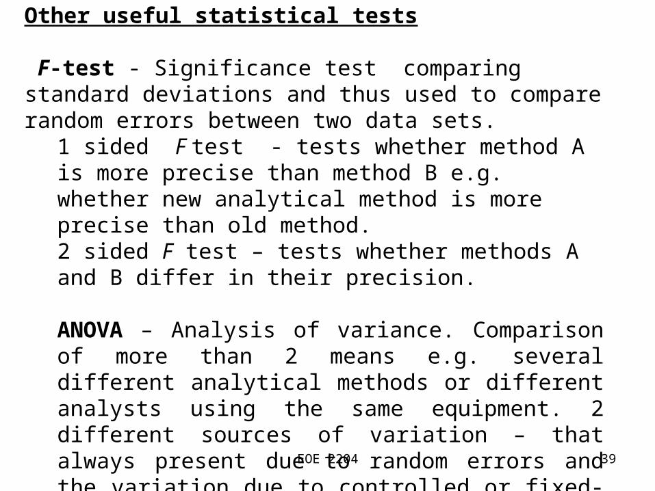
Other useful statistical tests

F-test - Significance test comparing standard deviations and thus used to compare random errors between two data sets.

1 sided F test - tests whether method A is more precise than method B e.g. whether new analytical method is more precise than old method.2 sided F test – tests whether methods A and B differ in their precision.

ANOVA – Analysis of variance. Comparison of more than 2 means e.g. several different analytical methods or different analysts using the same equipment. 2 different sources of variation – that always present due to random errors and the variation due to controlled or fixed-effect factors e.g. the solution storage conditions, the analytical method used or the analyst.

EOE 2204 40

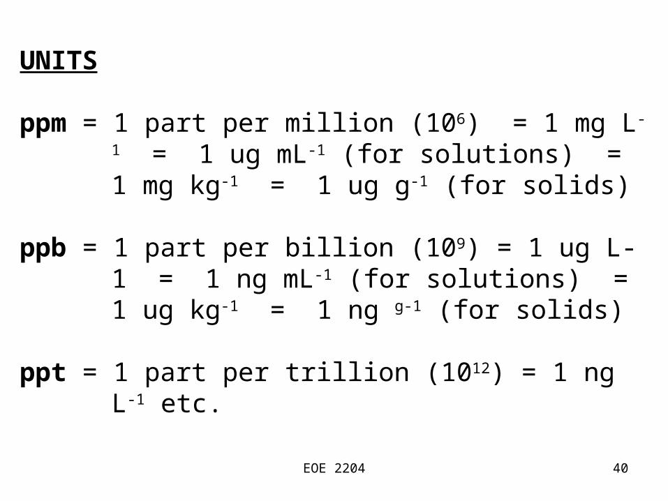
UNITS

ppm = 1 part per million (106) = 1 mg L-1 = 1 ug mL-1 (for solutions) = 1 mg kg-1 = 1 ug g-1 (for solids)

ppb = 1 part per billion (109) = 1 ug L-1 = 1 ng mL-1 (for solutions) = 1 ug kg-1 = 1 ng g-1 (for solids)

ppt = 1 part per trillion (1012) = 1 ng L-1 etc.

EOE 2204 41

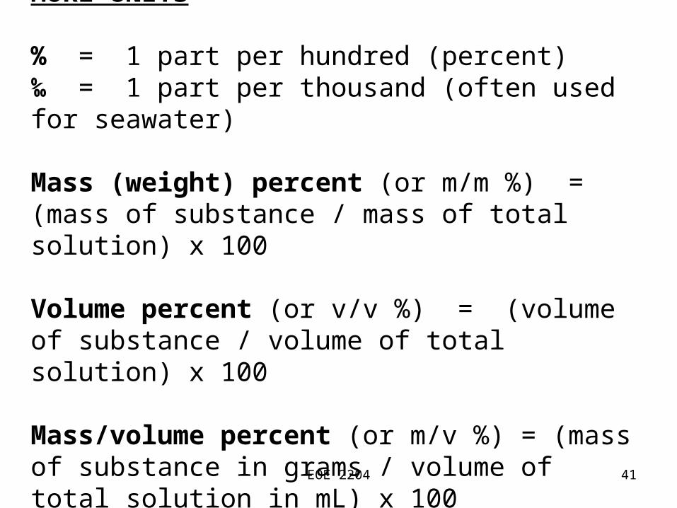
MORE UNITS

% = 1 part per hundred (percent)‰ = 1 part per thousand (often used for seawater)

Mass (weight) percent (or m/m %) = (mass of substance / mass of total solution) x 100

Volume percent (or v/v %) = (volume of substance / volume of total solution) x 100

Mass/volume percent (or m/v %) = (mass of substance in grams / volume of total solution in mL) x 100

EOE 2204 42

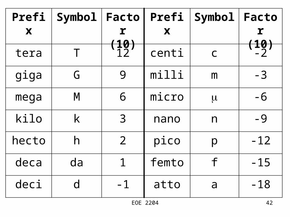
-18aatto-1ddeci

-15ffemto1dadeca

-12ppico2hhecto

-9nnano3kkilo

-6micro6Mmega

-3mmilli9Ggiga

-2ccenti12Ttera

Factor (10)

SymbolPrefixFactor (10)

SymbolPrefix

EOE 2204 43

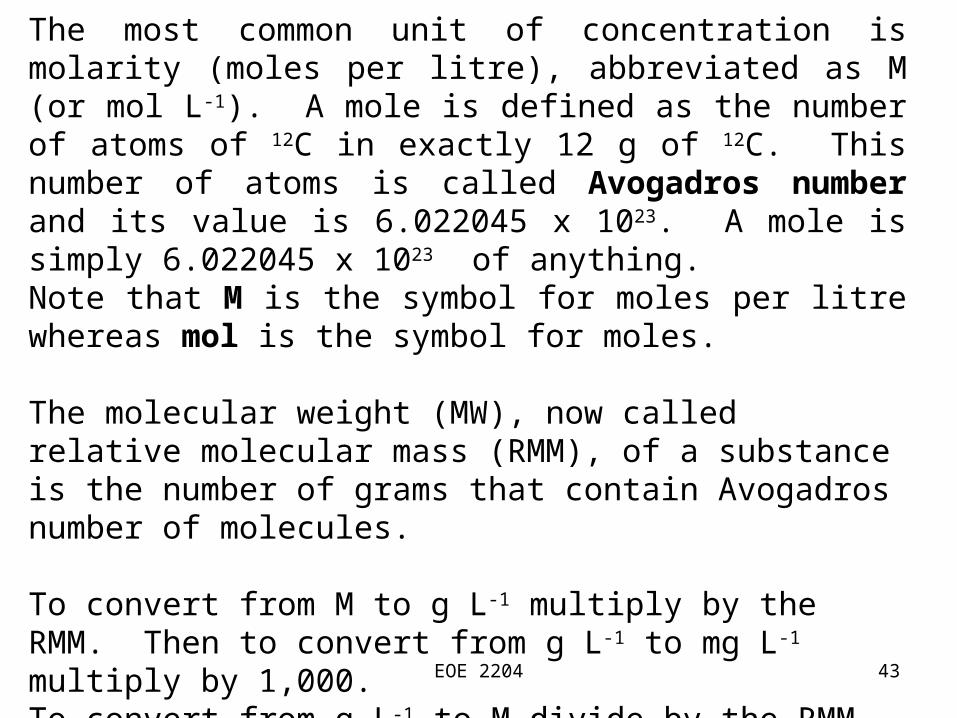
Molarity

The most common unit of concentration is molarity (moles per litre), abbreviated as M (or mol L-1). A mole is defined as the number of atoms of 12C in exactly 12 g of 12C. This number of atoms is called Avogadros number and its value is 6.022045 x 1023. A mole is simply 6.022045 x 1023 of anything. Note that M is the symbol for moles per litre whereas mol is the symbol for moles.

The molecular weight (MW), now called relative molecular mass (RMM), of a substance is the number of grams that contain Avogadros number of molecules.

To convert from M to g L-1 multiply by the RMM. Then to convert from g L-1 to mg L-1 multiply by 1,000.To convert from g L-1 to M divide by the RMM.

EOE 2204 44

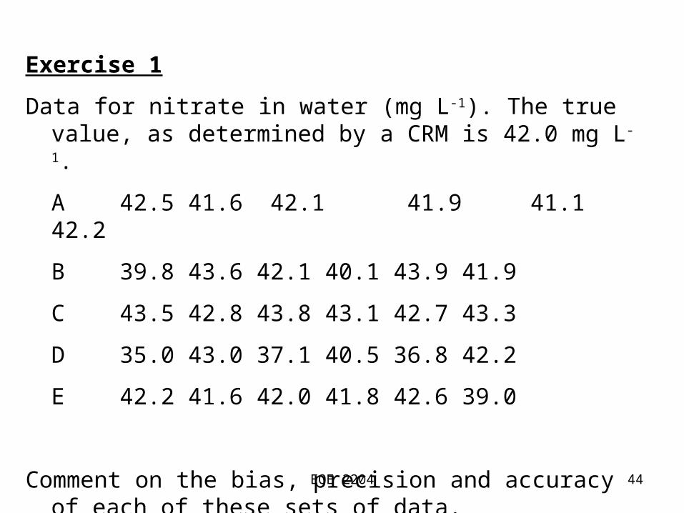
Exercise 1

Data for nitrate in water (mg L-1). The true value, as determined by a CRM is 42.0 mg L-1.

A 42.5 41.6 42.1 41.9 41.1 42.2

B 39.8 43.6 42.1 40.1 43.9 41.9

C 43.5 42.8 43.8 43.1 42.7 43.3

D 35.0 43.0 37.1 40.5 36.8 42.2

E 42.2 41.6 42.0 41.8 42.6 39.0

Comment on the bias, precision and accuracy of each of these sets of data.

EOE 2204 45

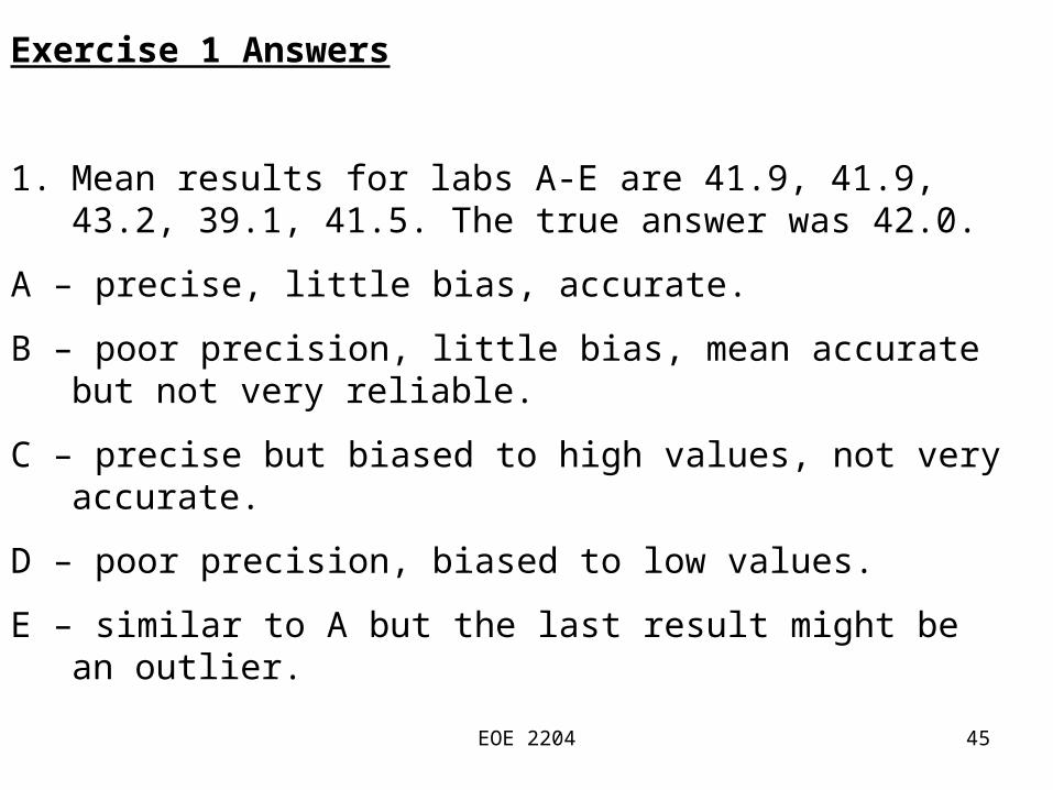
Exercise 1 Answers

1. Mean results for labs A-E are 41.9, 41.9, 43.2, 39.1, 41.5. The true answer was 42.0.

A – precise, little bias, accurate.

B – poor precision, little bias, mean accurate but not very reliable.

C – precise but biased to high values, not very accurate.

D – poor precision, biased to low values.

E – similar to A but the last result might be an outlier.

EOE 2204 46

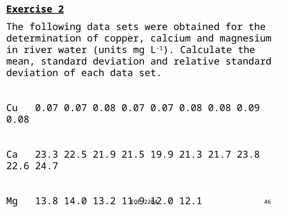
Exercise 2

The following data sets were obtained for the determination of copper, calcium and magnesium in river water (units mg L-1). Calculate the mean, standard deviation and relative standard deviation of each data set.

Cu 0.07 0.07 0.08 0.07 0.07 0.08 0.08 0.090.08

Ca 23.3 22.5 21.9 21.5 19.9 21.3 21.7 23.822.6 24.7

Mg 13.8 14.0 13.2 11.9 12.0 12.1

EOE 2204 47

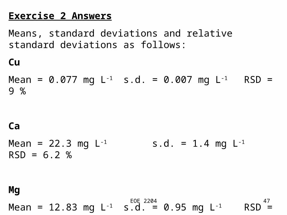
Exercise 2 Answers

Means, standard deviations and relative standard deviations as follows:

Cu

Mean = 0.077 mg L-1 s.d. = 0.007 mg L-1 RSD = 9 %

Ca

Mean = 22.3 mg L-1 s.d. = 1.4 mg L-1 RSD = 6.2 %

Mg

Mean = 12.83 mg L-1 s.d. = 0.95 mg L-1 RSD = 7.4 %

EOE 2204 48

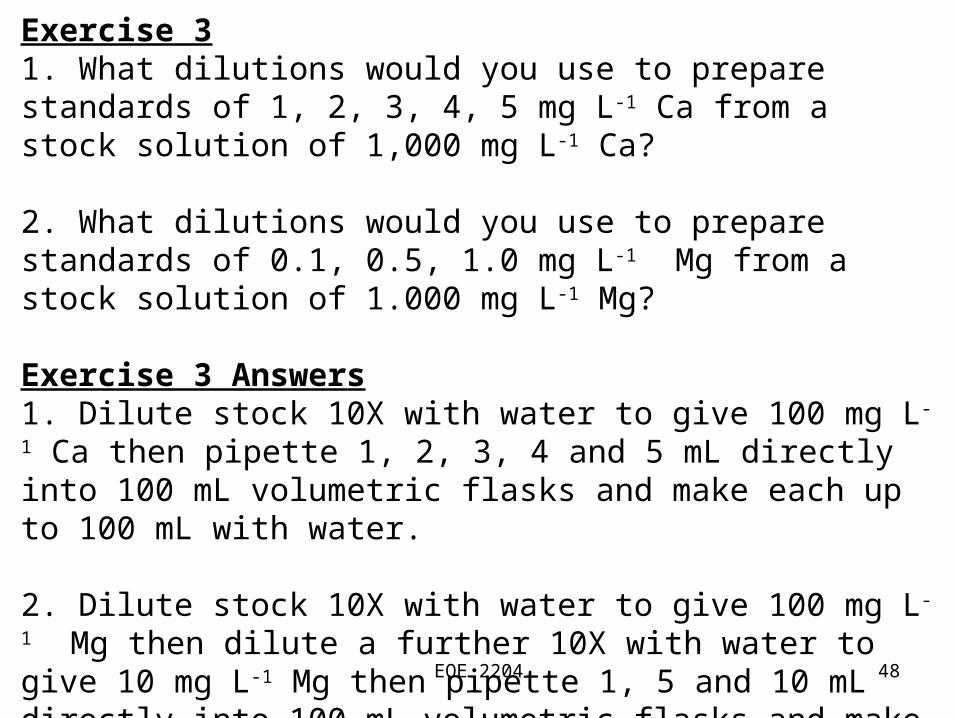
Exercise 31. What dilutions would you use to prepare standards of 1, 2, 3, 4, 5 mg L-1 Ca from a stock solution of 1,000 mg L-1 Ca?

2. What dilutions would you use to prepare standards of 0.1, 0.5, 1.0 mg L-1 Mg from a stock solution of 1.000 mg L-1 Mg?

Exercise 3 Answers1. Dilute stock 10X with water to give 100 mg L-1 Ca then pipette 1, 2, 3, 4 and 5 mL directly into 100 mL volumetric flasks and make each up to 100 mL with water.

2. Dilute stock 10X with water to give 100 mg L-1 Mg then dilute a further 10X with water to give 10 mg L-1 Mg then pipette 1, 5 and 10 mL directly into 100 mL volumetric flasks and make each up to 100 mL with water.Note: Always use ultrapure water e.g. from Milli-Q unit.

EOE 2204 49

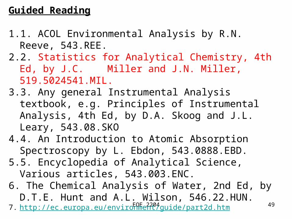
Guided Reading

1. 1. ACOL Environmental Analysis by R.N. Reeve, 543.REE.2. 2. Statistics for Analytical Chemistry, 4th Ed, by J.C. Miller

and J.N. Miller, 519.5024541.MIL.3. 3. Any general Instrumental Analysis textbook, e.g.

Principles of Instrumental Analysis, 4th Ed, by D.A. Skoog and J.L. Leary, 543.08.SKO

4. 4. An Introduction to Atomic Absorption Spectroscopy by L. Ebdon, 543.0888.EBD.

5. 5. Encyclopedia of Analytical Science, Various articles, 543.003.ENC.

6. The Chemical Analysis of Water, 2nd Ed, by D.T.E. Hunt and A.L. Wilson, 546.22.HUN.

7. http://ec.europa.eu/environment/guide/part2d.htm