RUN YOUR MODEL IN SIX STEPS

0) Before we start, most worksheets have special comments in cellsto help you out. You can recognize the comments by the red, small trianglein the upper-right hand corner like the one this cell has. Just move your pointer overthe cell to see the comment. To see all the comments, under the "View" menu, select the "Comments" menu item

1) Click the "model" worksheet tab below and enter your reactions in the cells provided.

2) Click the "CONTROL" worksheet tab below and click the "Make Species Spreadsheet from Model"

3) Click the "species" worksheet tab below and edit the initial concentrations, type a "Y" in the "Display Output ?" column for any species you wish to plot.

4) Click the "parm" worksheet tab and enter your desired simulation time in the DAYS,HOURS, MINUTES, SECONDS cells

5) Click the "CONTROL" worksheet tab below and click the "RUN" button. If you do not have a registration key, you will alsohave to press the ENTER key three times in the KINTECUS window(ie, click in the KINTECUS window, press ENTER three times)6) Click the "Plot Results" button on the CONTROL worksheet. That's it!!

8) OPTIONAL: If you wish to include temperature evolution plots and reverse rate autocalculations, type -THERM on the Kintecus Switches cell located on the CONTROL worksheet. See the excel file "Combustion_workbook_OH.xls" as an example!

9) OPTIONAL: If you wish to FIT experimental data to a model, enter your data in the "fitdata" worksheet, with Time(s) as the first column, first row. The species names should follow the Time(s) heading on the same row. Place your species/temperature data under the appropriate species column (if a species is missing data for a time point, place an “N” in the cell). Append a question mark, "?", to the end of values you wish for Kintecus to regress/fit. Type the additional switch "–FIT:2:3:FITDATA.TXT" in the KINTECUS SWITCHES cell located on the CONTROL worksheet. You can also try–FIT:1:3:FITDATA.TXT , -FIT:1:1:FITDATA.TXT and –FIT:2:1:FITDATA.TXT. Run Kintecus. You can see the "Enzyme_Regression_Fitting.xls" file as an example!!

10) OPTIONAL: If you wish to do sensitivity analysis just use the –SENSIT:1 on the commandline.

11) There are many other interesting things you can do with your model, so pleasebe sure to read the Kintecus.pdf documentation!

Kintecus Control Spreadsheet Page

Kintecus Registration/Unlocking Key (enter in the cell below)

Kintecus PATH (where Kintecus.exe and your files are located at. ie. C:\KINTECUS\ )C:\Kintecus\

Kintecus Switches -FIT:1:3 -ig:mass -FITSTAT:BOOT

0

NOTE** Most cells have comments which can be permanently shown on screen (like the one in this cell) by right clicking the cell and selecting "Show Comment", to hide, right click cell and select "Hide Comment"

I am using the German/Russian version of Excel =

This example shows you how to implement the BOOTSTRAP method in Kintecus to accurately evaluate the standard errors of whatever you are trying to fit/optimize. The BOOTSTRAP method wil take about 20 minutes on a Pentium IV.

James Ianni:

Once you click the RUN button below, Kintecus will Run. To stop Kintecus, press the ESCAPE key (Esc Key) FIRST! THEN type a Control-C (hold Ctrl key, press the C key) in the Kintecus Window to halt Kintecus.

This example shows you how to implement the BOOTSTRAP method in Kintecus to accurately evaluate the standard errors of whatever you are trying to fit/optimize. The BOOTSTRAP method wil take about 20 minutes on a Pentium IV.

James Ianni:

Once you click the RUN button below, Kintecus will Run. To stop Kintecus, press the ESCAPE key (Esc Key) FIRST! THEN type a Control-C (hold Ctrl key, press the C key) in the Kintecus Window to halt Kintecus.

# Non-competitive Inhibition# of an enzymatic reaction# Example spreadsheet. You can see comments by moving pointer above the red triangles## 5e6 is the EXACT ANSWER for the rate constant below!1e7? E+S==>ES# 66666.66667 is the EXACT ANSWER for the rate constant below!k1*0.0133333 ES ==> E+S# 8.50E+06 is the EXACT ANSWER for the rate constant below!

8.50E+06 E+I==>EI112687259.71099 EI==>E+I

# 9.57E61e7? ES+I==>EISk5*0.395257 EIS==>ES+I# 5.53E7, 3.09E61? EI+S==>EISk7*0.05596 EIS==>EI+S# 7.13E+6, 2.01E+5

7.13E+06 EI+P==>EIS2.01E+05 EIS==>EI+P

# 1.14E51.14E+05 ES==>E+P

END

Equilibrium Constants1/Keq

75 0.013333

0.07543 13.25732

2.53 0.395257

17.87 0.05596

35.5 0.028169

# Species Description Spreadsheet# Species Residence Initial Display Output External Species Special# Time in CSTR(s) Conc. (Y/N) ? Conc. Directives ? (/N) E 0 4.00E-09 YES 0 No S 0 6.00E-02 YES 0 No ES 0 0 YES 0 No I 0 4.00E-05 YES 0 No EI 0 0 YES 0 No EIS 0 0 YES 0 No P 0 0 YES 0 No END ####

Constant File?(Filename/#/No) CommentsNoNoNoNoNoNoNo

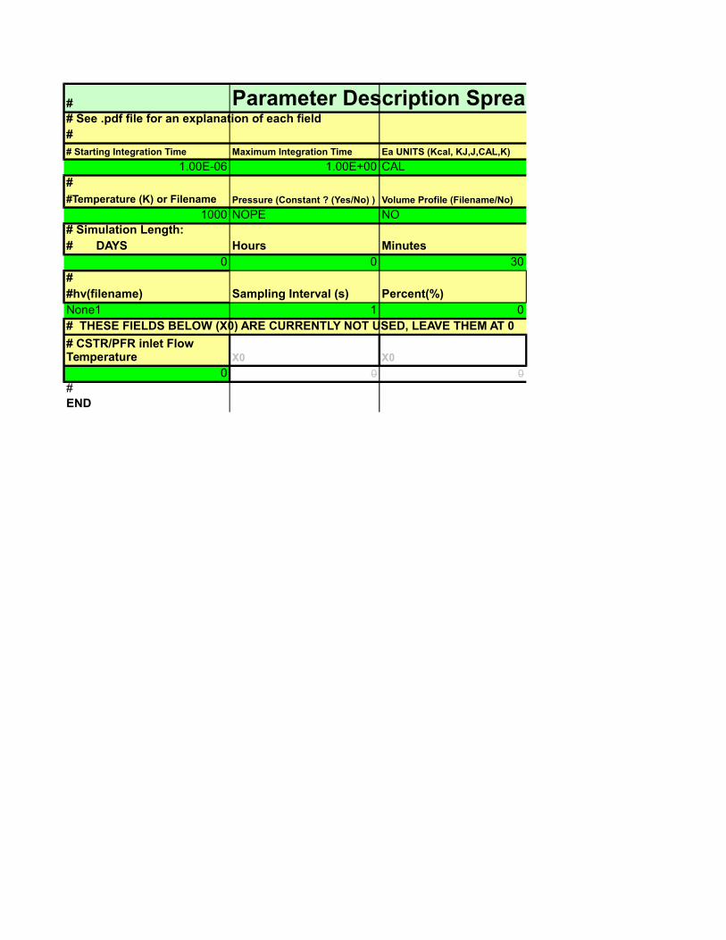
# Parameter Description SpreadSheet# See .pdf file for an explanation of each field#

# Starting Integration Time Maximum Integration Time Ea UNITS (Kcal, KJ,J,CAL,K)

1.00E-06 1.00E+00 CAL##Temperature (K) or Filename Pressure (Constant ? (Yes/No) ) Volume Profile (Filename/No)

1000 NOPE NO# Simulation Length:# DAYS Hours Minutes

0 0 30# #hv(filename) Sampling Interval (s) Percent(%)None1 1 0# THESE FIELDS BELOW (X0) ARE CURRENTLY NOT USED, LEAVE THEM AT 0

X0 X0

0 0 0

#END

# CSTR/PFR inlet Flow Temperature

Parameter Description SpreadSheet

Conc. Units(moles/L, moles/cc, molecules/cc) X0

MOLES/LITER 0

External Heat Source/Sink # OR Profile (Filename)

OR Condutance:Extern. Temp OR Conductance:Ext.Temp.X0

No 0

Seconds PicoSeconds0.00E+00 0

Accuracy X0

1.00E-08 0

X0 X0

0 0

Time(s) E S ES EIS ## fitdata worksheet contains your experimental or "fabricated" data# for which Kintecus will fit your selected parameters to# An 'N' or 'NaN' or 'None' in a cell represents NO data for that species at that time# IMPORTANT NOTE!, the excel macros "latch" on column headings above# so you should ONLY have the Time(s) and the name of each species in row 1#3.55E+00 1.52E-09 5.90E-02 2.48E-09 1.38E-132.38E+01 1.62E-09 5.34E-02 2.38E-09 1.33E-135.33E+01 1.77E-09 4.56E-02 2.23E-09 1.24E-138.28E+01 1.94E-09 3.84E-02 2.06E-09 1.14E-131.12E+02 2.13E-09 N 1.87E-09 1.04E-131.42E+02 2.33E-09 N 1.67E-09 9.24E-141.71E+02 2.55E-09 N 1.45E-09 8.05E-142.01E+02 N N 1.23E-09 6.83E-142.30E+02 N N 1.01E-09 N2.60E+02 N N 8.13E-10 N2.89E+02 N N 6.33E-10 N3.19E+02 N N 4.80E-10 N3.48E+02 N 3.54E-03 3.56E-10 N3.78E+02 N 2.51E-03 2.59E-10 N4.07E+02 N 1.76E-03 1.86E-10 N4.37E+02 N 1.23E-03 1.32E-10 N4.66E+02 N 8.60E-04 9.29E-11 N4.96E+02 N 5.97E-04 6.50E-11 N5.25E+02 N 4.14E-04 4.53E-11 N5.55E+02 N 2.86E-04 3.14E-11 N5.84E+02 N 1.98E-04 N N6.14E+02 N 1.37E-04 N N6.43E+02 N 9.44E-05 N 1.30E-156.73E+02 N 6.52E-05 N 1.12E-157.02E+02 3.99E-09 4.51E-05 N 1.00E-157.32E+02 4.00E-09 3.12E-05 N 9.18E-167.61E+02 4.00E-09 2.16E-05 N 8.60E-167.91E+02 4.00E-09 1.49E-05 N 8.20E-168.21E+02 4.00E-09 1.04E-05 N 7.92E-168.50E+02 4.00E-09 7.24E-06 N 7.73E-168.80E+02 4.00E-09 5.07E-06 N 7.60E-169.09E+02 4.00E-09 3.58E-06 N 7.51E-169.39E+02 4.00E-09 2.55E-06 N 7.45E-169.68E+02 4.00E-09 1.84E-06 N 7.40E-169.98E+02 N 1.35E-06 N 7.37E-161.03E+03 N 1.01E-06 N 7.35E-161.06E+03 N 7.76E-07 N 7.34E-161.09E+03 N 6.15E-07 N 7.33E-161.12E+03 N 5.05E-07 7.10E-14 7.32E-161.15E+03 N 4.28E-07 6.26E-14 7.32E-161.17E+03 N 3.76E-07 5.68E-14 7.32E-161.20E+03 N 3.40E-07 5.28E-14 7.31E-16

1.23E+03 N 3.15E-07 5.00E-14 7.31E-161.26E+03 N 2.97E-07 4.81E-14 N1.29E+03 N 2.86E-07 4.68E-14 N1.32E+03 4.00E-09 2.77E-07 4.59E-14 N1.35E+03 4.00E-09 2.72E-07 4.53E-14 N1.38E+03 4.00E-09 2.68E-07 4.49E-14 N1.41E+03 4.00E-09 2.65E-07 4.46E-14 N1.44E+03 4.00E-09 2.63E-07 4.44E-14 N1.47E+03 4.00E-09 2.62E-07 4.42E-14 N1.50E+03 4.00E-09 2.61E-07 4.41E-14 N1.53E+03 4.00E-09 2.61E-07 4.41E-14 N1.56E+03 4.00E-09 2.60E-07 4.40E-14 N1.59E+03 4.00E-09 2.60E-07 4.40E-14 N1.62E+03 4.00E-09 2.60E-07 4.40E-14 N1.65E+03 4.00E-09 N 4.39E-14 N1.68E+03 4.00E-09 N 4.39E-14 N1.71E+03 4.00E-09 N 4.39E-14 N1.74E+03 4.00E-09 N 4.39E-14 7.31E-161.76E+03 4.00E-09 N 4.39E-14 7.31E-161.80E+03 4.00E-09 N 4.39E-14 7.31E-16

END