ENVIRONMENTAL TRACERS IN GROUNDWATER ... TRACERS IN GROUNDWATER OF THE SALT BASIN, NEW MEXICO, AND...

ENVIRONMENTAL TRACERS IN GROUNDWATER

OF THE SALT BASIN, NEW MEXICO, AND

IMPLICATIONS FOR WATER RESOURCES

By

SOPHIA CARMELITA SIGSTEDT

Master of Science in Hydrology

New Mexico Institute of Mining and Technology

Socorro, New Mexico

2010

Submitted to the Faculty of the

Earth and Environmental Science Department of the

New Mexico Institute of Mining and Technology

in partial fulfillment of

the requirements for

the Degree of

MASTER OF SCIENCE IN HYDROLOGY

August, 2010

ii

ENVIRONMENTAL TRACERS IN GROUNDWATER

OF THE SALT BASIN, NEW MEXICO, AND

IMPLICATIONS FOR WATER RESOURCES

Thesis Approved:

Dr. Fred M. Phillips

Thesis Adviser

Dr. Penelope J. Boston

Dr. Mark Person

Dr. David B. Johnson

Dean of Graduate Studies

iii

ACKNOWLEDGMENTS

My thanks go out to my field partner Andre Ritchie who braved the dust storms, gas leaks, flat

tires, javalinas, and all the other unexpected obstacles the Salt Basin had to throw at us.

I want to thank my Advisor Dr. Fred Phillips who gave me the wonderful opportunity of working

on this adventurous project. I truly appreciate his attention to detail and ability to patiently

explain everything from comma placement to cosmic rays.

Thanks to my committee members, Dr. Mark Person and Dr. Penny Boston, for their

encouragement and perspective.

A special thanks to Stacy Timmons and Lewis Land, from the New Mexico Bureau of Geology

and Mineral Resources, particularly for their guidance with sampling during the early stages of

the field work for this project.

I want to thank Andy Campbell not only for the many water analyses he ran for this project, but

also for his availability to answer questions and guide me toward the next step.

Thanks to my research group for their input and support. I especially want to thank Jeremiah

Morse who was working on a similar project when I started and kept me going in the right

direction. I also want to thank Marty Frisbee for being so generous with his time and ideas.

This Salt Basin study is part of a much larger project to assess the Salt Basin Aquifer system. It

was really interesting working on a project being analyzed from so many different angles. I want

to thank everyone we worked with: Bill Miller (Engineers), Craig Roepke (ISC), John Kay (D&B

Stephens), David Jordan (Intera), Penny Boston (NMT), Todd umstot (D&B Stephens), Jan

Hendrickx (NMT), Anne Tillery (USGS), and Steve Finch (Shomaker & Assoc.)

iv

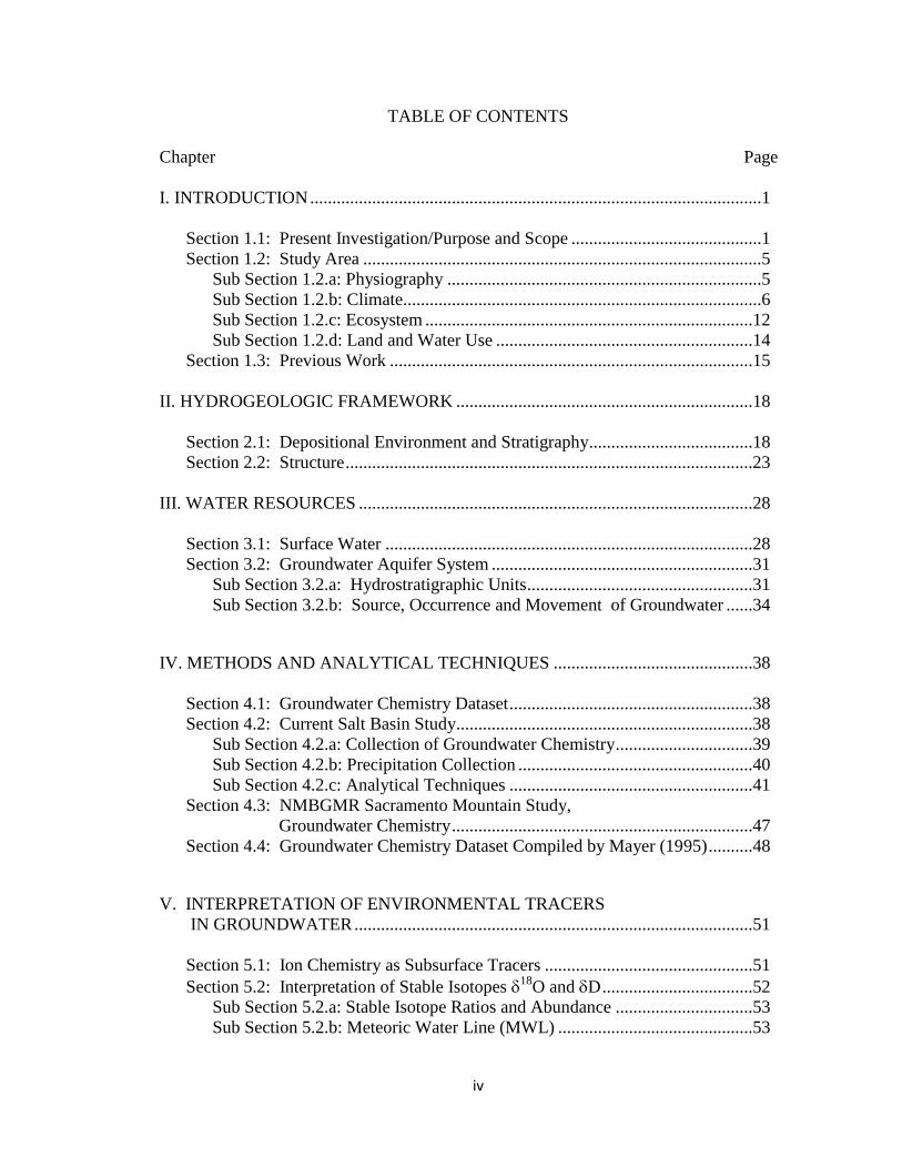
TABLE OF CONTENTS

Chapter Page

I. INTRODUCTION ......................................................................................................1

Section 1.1: Present Investigation/Purpose and Scope ...........................................1

Section 1.2: Study Area ..........................................................................................5

Sub Section 1.2.a: Physiography .......................................................................5

Sub Section 1.2.b: Climate.................................................................................6

Sub Section 1.2.c: Ecosystem ..........................................................................12

Sub Section 1.2.d: Land and Water Use ..........................................................14

Section 1.3: Previous Work ..................................................................................15

II. HYDROGEOLOGIC FRAMEWORK ...................................................................18

Section 2.1: Depositional Environment and Stratigraphy.....................................18

Section 2.2: Structure ............................................................................................23

III. WATER RESOURCES .........................................................................................28

Section 3.1: Surface Water ...................................................................................28

Section 3.2: Groundwater Aquifer System ...........................................................31

Sub Section 3.2.a: Hydrostratigraphic Units...................................................31

Sub Section 3.2.b: Source, Occurrence and Movement of Groundwater ......34

IV. METHODS AND ANALYTICAL TECHNIQUES .............................................38

Section 4.1: Groundwater Chemistry Dataset .......................................................38

Section 4.2: Current Salt Basin Study...................................................................38

Sub Section 4.2.a: Collection of Groundwater Chemistry ...............................39

Sub Section 4.2.b: Precipitation Collection .....................................................40

Sub Section 4.2.c: Analytical Techniques .......................................................41

Section 4.3: NMBGMR Sacramento Mountain Study,

Groundwater Chemistry ....................................................................47

Section 4.4: Groundwater Chemistry Dataset Compiled by Mayer (1995) ..........48

V. INTERPRETATION OF ENVIRONMENTAL TRACERS

IN GROUNDWATER ..........................................................................................51

Section 5.1: Ion Chemistry as Subsurface Tracers ...............................................51

Section 5.2: Interpretation of Stable Isotopes 18

O and D ..................................52

Sub Section 5.2.a: Stable Isotope Ratios and Abundance ...............................53

Sub Section 5.2.b: Meteoric Water Line (MWL) ............................................53

v

Chapter Page

Sub Section 5.2.c: Factors Controlling the Isotopic

Composition of Precipitation .............................................55

Sub Section 5.2.d: Identifying Sources of Recharge .......................................57

Section 5.3: Tritium as an Environmental Tracer .................................................59

Section 5.4: Radiocarbon (14

C) Dating Groundwater .........................................60

Sub Section 5.4.a: Natural Abundances of Carbon

and 14

C Radioactive Decay ..............................................60

Sub Section 5.4.b: Concepts in Deriving Radiocarbon (14

C)

Age of Groundwater .........................................................61

Sub Section 5.4.c: Interpretation of Radiocarbon (14

C)

Age of Groundwater ..........................................................62

Section 5.5: 34

SO4 as a Lithologic Tracer ...........................................................64

VI. GROUNDWATER SYSTEM CHARACTERIZATION .....................................66

Section 6.1: Groundwater Chemistry ....................................................................66

Sub Section 6.1.a: Groundwater Temperature, Conductivity, and TDS ..........68

Sub Section 6.1.b: Major Cations ....................................................................73

Sub Section 6.1.c: Major Anions .....................................................................80

Sub Section 6.1.d: Minor Constituents ............................................................86

Section 6.2: Groundwater Chemistry Evolution ...................................................88

Sub Section 6.2.a: Solute Sources and Sinks in the Aquifer System ...............88

Sub Section 6.2.b: Evidence for Dedolomitization ..........................................93

Sub Section 6.2.c: Water Chemistry of Otero Mesa ........................................96

Sub Section 6.2.d: Brine Evolution..................................................................97

Section 6.3: Geochemical Reactions and Mass Transfer .......................................98

Section 6.4: Chemical and Mineralogical Comparison using SaltNorm………..105

Section 6.5: Salt Basin Solute Controls by Faults and Structural Features….….109

VII. STABLE ISOTOPES AND THEIR IMPLICATIONS FOR RECHARGE .....115

Section 7.1: Recharge Environment ...................................................................115

Section 7.2: Stable Isotope Distribution .............................................................117

Section 7.3: Implication for Guadalupe M. Recharge .........................................121

Section 7.4: Implication for Paleo-groundwater Recharge ..................................122

Section 7.5: Principal Component Analysis/EMMA ..........................................131

VIII. GEOCHEMICAL MODELING TO ESTIMATE RECHARGE- 14

C .............137

Section 8.1: Radiocarbon Dating in GW Systems ..............................................137

Section 8.2: Definition of Recharge Chemistry ..................................................138

vi

Chapter Page

Section 8.3: Dedolomitization Reaction Model .........................................................139

Sub Section 8.3.a: Modeling Strategy............................................................140

Sub Section 8.3.b: Modeling Parameter and Constraints ..............................141

Sub Section 8.3.c: Groundwater Age Distribution ........................................145

Section 8.4: NETPATH Geochemical Model ............................................................150

Sub Section 8.4.a: Modeling Strategy............................................................151

Sub Section 8.4.b: Modeling Parameter and Constraints ..............................152

Sub Section 8.4.c: Groundwater age distribution ..........................................156

Section 8.5: Implications for Recharge from Radiocarbon Dating ............................162

Sub Section 8.5.a: Seepage Velocity/Hydraulic Conductivity ......................162

Sub Section 8.5.b: Piston-flow approximation ..............................................166

Sub Section 8.5.c: Groundwater Flux Calculation.........................................167

Sub Section 8.5.d: Water Age Correlations with Solute Concentration ........171

IX. CONCLUSION...................................................................................................174

REFERENCES ..........................................................................................................177

APPENDICES ...........................................................................................................191

vii

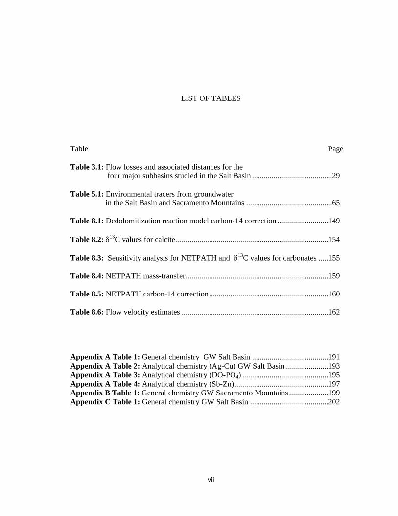
LIST OF TABLES

Table Page

Table 3.1: Flow losses and associated distances for the

four major subbasins studied in the Salt Basin .........................................29

Table 5.1: Environmental tracers from groundwater

in the Salt Basin and Sacramento Mountains ............................................65

Table 8.1: Dedolomitization reaction model carbon-14 correction ..........................149

Table 8.2: 13

C values for calcite ..............................................................................154

Table 8.3: Sensitivity analysis for NETPATH and 13

C values for carbonates .....155

Table 8.4: NETPATH mass-transfer .........................................................................159

Table 8.5: NETPATH carbon-14 correction .............................................................160

Table 8.6: Flow velocity estimates ...........................................................................162

Appendix A Table 1: General chemistry GW Salt Basin .......................................191

Appendix A Table 2: Analytical chemistry (Ag-Cu) GW Salt Basin ......................193

Appendix A Table 3: Analytical chemistry (DO-PO4) ............................................195

Appendix A Table 4: Analytical chemistry (Sb-Zn) ................................................197

Appendix B Table 1: General chemistry GW Sacramento Mountains ....................199

Appendix C Table 1: General chemistry GW Salt Basin ........................................202

viii

LIST OF FIGURES

Figure Page

1.1 Salt Basin study area with important physiographic features and locations. ........2

1.2 Minimum annual temperature distribution in the Salt Basin. ...............................7

1.3 Maximum annual temperature distribution in the Salt Basin. ..............................8

1.4 Average annual temperature distribution in the Salt Basin ..................................9

1.5 Average annual precipitation in the Salt Basin ...................................................10

1.6 Sacramento Mountains, Cloudcroft NM, monthly climate record .....................11

1.7 Eco-Regions of the Salt Basin ............................................................................13

2.1 General stratigraphic column for the Salt Basin region .....................................19

2.2 Surface geology of the northern Salt Basin ........................................................22

2.3 Structural fault zones for the Salt Basin .............................................................24

2.3 Tectonic structural features of the Salt Basin during the Cenozoic ....................26

3.1 Salt Basin sub-watersheds...................................................................................30

3.2 Groundwater movement and water elevation contours ......................................37

4.1 Salt Basin well sample locations.........................................................................46

4.2 Distribution of comprehensive well water chemistry dataset

used for analysis for the Salt Basin .....................................................................50

5.1 The relationship between D and 18O of meteoric water,

as well as deviations from the MWL ..................................................................54

6.1 Distribution of sample points used for geochemical modeling

through general sub-regions of the Salt Basin ....................................................67

6.2 Relationship of measured groundwater and surface air temperature ..................69

6.3 Measured groundwater temperatures to elevation ..............................................69

6.4 Map of well water temperature ...........................................................................70

6.5 Measured groundwater TDS in relation to northing ...........................................71

6.6 Map of well water TDS concentration ................................................................72

6.7 Measured groundwater magnesium concentration in relation to northing .........73

6.8 Measured groundwater calcium concentration in relation to northing ...............74

6.9 Measured groundwater sodium concentration in relation to northing ................74

6.10 Measured groundwater potassium concentration in relation to northing..........75

ix

Figure Page

6.11 Map of magnesium concentration .....................................................................77

6.12 Map of sodium concentration ...........................................................................78

6.13 Map of calcium concentration ..........................................................................79

6.14 Measured groundwater chloride concentration in relation to northing .............81

6.15 Measured groundwater sulfate concentration in relation to northing ...............81

6.16 Measured groundwater bicarbonate concentration in relation to northing .......82

6.17 Map of chloride concentration ..........................................................................83

6.18 Map of sulfate concentration ............................................................................84

6.19 Map of bicarbonate concentration ....................................................................85

6.20 Measured groundwater fluoride concentration in relation to northing .............86

6.21 Measured groundwater silica concentration in relation to northing .................87

6.22 Measured groundwater strontium concentration in relation to northing ..........87

6.23 Molar ratios of Ca+Mg/HCO3 ..........................................................................89

6.24 Molar ratios of Ca+Mg-SO4/HCO3 ...................................................................90

6.25 Molar ratios of Na / Cl ......................................................................................92

6.26 Piper diagram of Salt Basin well chemistry ......................................................95

6.27 Piper diagram of groundwater chemistry of Pahasapa Limestone

Madison Aquifer ...............................................................................................96

6.28 Saturation index for gypsum ...........................................................................100

6.29 Saturation index for dolomite .........................................................................100

6.30 Saturation index for calcite .............................................................................101

6.31 Secondary calcite in thin sections from the San Andres .................................102

6.32 Trend in log partial pressure of carbon dioxide ..............................................103

6.33 Trend in pH .....................................................................................................104

6.34 Trend in Mg/Ca ratio ......................................................................................105

6.35 SaltNorm distribution for the Salt Basin .........................................................107

6.36 SaltNorm distribution for the Madison Aquifer..............................................109

6.37 Association of magnesium concentration and

major faults and structural .............................................................................113

6.38 Association of sulfate concentration and

major faults and structural .............................................................................114

7.1 Oxygen and deuterium stable isotope distribution ...........................................118

7.2 Tritium concentration distribution ....................................................................123

7.3 Tritium versus pmc ...........................................................................................124

7.4 Deuterium versus pmc ......................................................................................125

7.5 Isotopic shift projected by evaporation line ......................................................126

7.6 Isotopic depletion comparison ..........................................................................128

7.7 Measured groundwater oxygen-18 in relation to northing ...............................129

x

Figure Page

7.8 Measured groundwater deuterium in relation to northing ................................130

7.9 Salt Basin well water mixing space (EMMA) ..................................................133

7.10 Crow Flats well water mixing space (EMMA) ...............................................134

7.11 Dell City area well water mixing space (EMMA) ..........................................134

7.12 Distribution of end-member contribution .......................................................136

8.1 Flow paths used for geochemical modeling......................................................142

8.2 Magnesium modeling trends fit ........................................................................143

8.3 Bicarbonate modeling trends fit ........................................................................143

8.4 13

C modeling trends fit ......................................................................................144

8.5 14

C modeling trend fit .......................................................................................144

8.6 Observed versus measured 13

C dedolomitization model flow path 1 ...............146


C dedolomitization model flow path 2 ...............147

8.8 Apparent age distribution dedolomitization model ...........................................148


C NETPATH model in relation to northing .......157

8.10 Apparent age distribution NETPATH model .................................................161

8.11 Distance down flow path vs groundwater age ................................................163

8.12 Plot of average porosity versus depth .............................................................164

8.13 Hydraulic conductivity comparison ................................................................165

8.14 Pison-flow approximation ...............................................................................166

8.15 Pison-flow compared to NETPATH GW age approximation ........................167

8.16 Cross-sectional width for flux calculation ......................................................168

8.17 Groundwater sulfur-34 isotope ratios in relation to northing .........................169

8.18 Stratigraphic cross-section down flow path ....................................................170

8.19 Magnesium as a function of groundwater age ................................................172

8.20 Sulfate as a function of groundwater age ........................................................172

1

CHAPTER I

INTRODUCTION

Section 1.1: Present Investigation/Purpose and Scope

The Salt Basin in southern New Mexico (fig. 1.1) is an example of a groundwater

system that is heavily pumped, primarily for agricultural purposes, while the recharge

rates and storage capacity of the basin are not fully understood. Current figures for

recharge to the Salt Basin groundwater system range from 15,000-100,000 acre-ft/yr.

These estimates came out following the designation of the Salt Basin by the State

Engineer in 2000. They are based on a series of studies which were compiled, along with

each author‘s estimate, primarily in two reports: one by John Shomaker & Associates,

Inc., and the other by Sandia National Labs and the USGS (Finch, 2002; Huff and Chace

2006). South of the New Mexico portion of the Salt Basin, just below the NM-TX state

line, is the Dell City Irrigation District. In 2000 as much as 210,000 acre-ft of water was

used to irrigate about 50,000 acres of farm land in Dell City (Chace and Huff, 2006).

While current rates of pumping in Dell City are at least half that, competing interests

have arisen in the basin as a future water source. resulting in three applications over the

appropriation of the Salt Basin groundwater; two of which ask the Office of the State

Engineer for the designation of almost 100,000 acre-ft/yr, each (Buynek, 2007). It is

apparent that the large uncertainty regarding the amount of recharge to the Salt Basin

constitutes a serious impediment to proper resource management, for which the amount

of recharge as well as spatial distribution need to be better constrained.

2

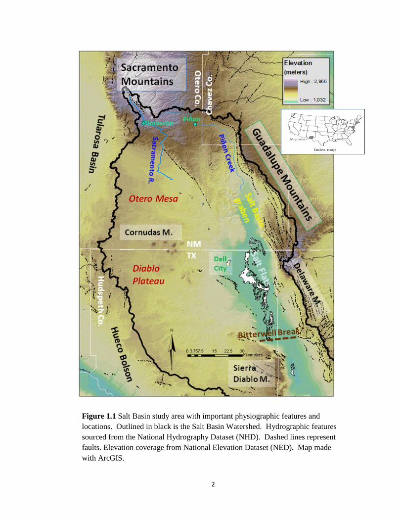
Figure 1.1 Salt Basin study area with important physiographic features and

locations. Outlined in black is the Salt Basin Watershed. Hydrographic features

sourced from the National Hydrography Dataset (NHD). Dashed lines represent

faults. Elevation coverage from National Elevation Dataset (NED). Map made

with ArcGIS.

3

A regional scale integrated, conceptual model of the Salt Basin groundwater

system is lacking. The Salt Basin can generally be typified as a karstic aquifer, for which

flow paths and permeability are difficult to quantify because of extensive small-scale

variability in porosity and fracture-dominated connectivity (Bakalowicz, 2005).

Understanding dominant trends in basin-scale permeability associated with the tectonic

forcing and depositional environment during the formation of the Salt Basin is a critical

foundation for the hydrogeologic conceptual model. However, due to the small number

of wells and high degree of natural variability in permeability and other hydrologic

properties, well hydraulics are of limited utility in basin analysis. In this situation, basin-

scale hydrodynamics of the system can be effectively characterized by means of

environmental tracers. These are naturally present in the groundwater system and can

illustrate integrated hydrologic behavior along flow paths. In this study, a suite of

environmental tracers have been quantified in the Salt Basin groundwater system in order

to obtain information on sources of recharge, estimates of recharge rates, flow paths, flow

rates, and sources of solutes in the groundwater.

Groundwater chemistry evolves with time and distance along a flow path. The

chemical evolution is determined by geochemical mass transfer between the groundwater

and the lithology of the aquifer units. Understanding the dominant controls on this

chemical evolution can elucidate flow path directions as well as sources of solutes in the

groundwater.

Two important tracers we have employed are the stable isotope ratios of oxygen

(18

O/16

O) and deuterium ( 2H/

1H). These isotopes, present in the molecules of

groundwater that originate as atmospheric precipitation, are a function of precipitation

4

conditions such as amount of precipitation, elevation, and temperature, and are thus a

reflection of the conditions under which recharge occurs. This connection allows for

their application in determining sources of recharge, as well as flow paths from the

source and evaporation effects. Stable isotope ratios of 18

O/16

O (18

O) and 2H/

1H (D)

have also been used in groundwater studies to reveal evidence for the presence of very

old water recharged into the aquifer during very different local climate conditions such as

during the Pleistocene.

Recharge estimates for the Salt Basin will primarily be determined by dating the

groundwater using carbon-14 which is subject to radioactive decay. For the most

accurate apparent ages the carbon-14 measured from the groundwater needs to be

corrected for the dilution of atmospheric CO2 by rock/water interactions with dead rock

carbon along the flow path. Geochemical mass transfer reactions are defined based on an

understanding of the mineralogy of the aquifer units, as well as the geochemical

evolution of the Salt Basin groundwater. Subsurface reaction models based on the

geochemistry can be used to correct the carbon-14. Seepage velocities can be estimated

using groundwater residence times determined from the radiocarbon dating along well

defined flow paths. With estimates for flow velocity and porosity groundwater flux can

be calculated across a given subsurface cross-section. This in turn, can be related to the

recharge flux entering the Salt Basin along primary flow paths. Understanding rates of

recharge in the Salt Basin is a critical component for sustainable resource management.

5

Section 1.2: Study Area

The northern portion of the Salt Basin (fig 1.1) is located primarily in

southeastern Otero County New Mexico, and Hudspeth County Texas. At the northern

boundary of the Salt Basin are the Sacramento Mountains which extend slightly into the

basin. The western margin of the Salt Basin in New Mexico is located where the Otero

Mesa uplift meets the Tularosa Basin; in Texas the western margin is the Diablo Plateau.

To the east the Salt Basin is bounded by the Guadalupe Mountains and Brokeoff

Mountains in New Mexico; these extend south into the Delaware Mountains in Texas.

The southern boundary for the New Mexico portion of the Salt Basin, based on its

designation for the N.M. State Engineer‘s Office is the New Mexico, Texas state line.

However, hydrologically, the southern boundary for the northern portion of the Salt Basin

is better defined by the beginnings of the Sierra Diablo Mountains in Texas, which

represent a surface-water drainage divide and a fault zone which divides the subsurface

flow (Kreitler, 1990). In its entirety, the Salt Basin extends through Texas and into

Mexico. Because the northern portion of the Salt Basin is a hydrologically closed basin,

natural groundwater discharge takes place north of the groundwater divide in a series of

playas known as the Salt Flats.

Section 1.2.a: Physiography

Most of the defining topographic features are a result of crustal extension

associated with the North American Basin and Range Province; of which the Salt Basin

(fig 1.1) is part of the eastern extent. The typical east-west crustal deformation results in

downfaulted valleys, or grabens, and upfaulted mountains. The Salt Basin graben that

6

lies between the Sacramento Mountains, the Guadalupe Mountains and the Otero Mesa,

is a result of this type of tectonic activity. The floor of the Salt Basin graben is almost

planar, dipping gently to the south between the elevations of about 1,000 and 1,100 m

(Mayer, 1995). The elevations of the surrounding uplands are at about 2,500-2,900 m for

the Sacramento Mountains, 1,500-2,100 m for Otero Mesa, and 1,400- 2,600 m for the

Guadalupe Mountains. The southern extension of the Sacramento Mountain uplift that

lies east of Otero Mesa and meets the northern boundary of the Salt Basin graben is the

Chert Plateau (Mayer, 1995). The topography of the Chert Plateau and eastern Otero

Mesa is characterized by many low elevation hills that focus surface water flow, creating

distinct draws that wind through the hills. These shallow, broad, natural watercourses

open out and disappear as they meet the flats of the Salt Basin graben. West of the Salt

Basin graben, in the southern extent of the Otero Mesa, are several Tertiary igneous

intrusions known as the Cornudas Mountains that form distinct and isolated peaks rising

to about 2,100 m.

Section 1.2.b: Climate

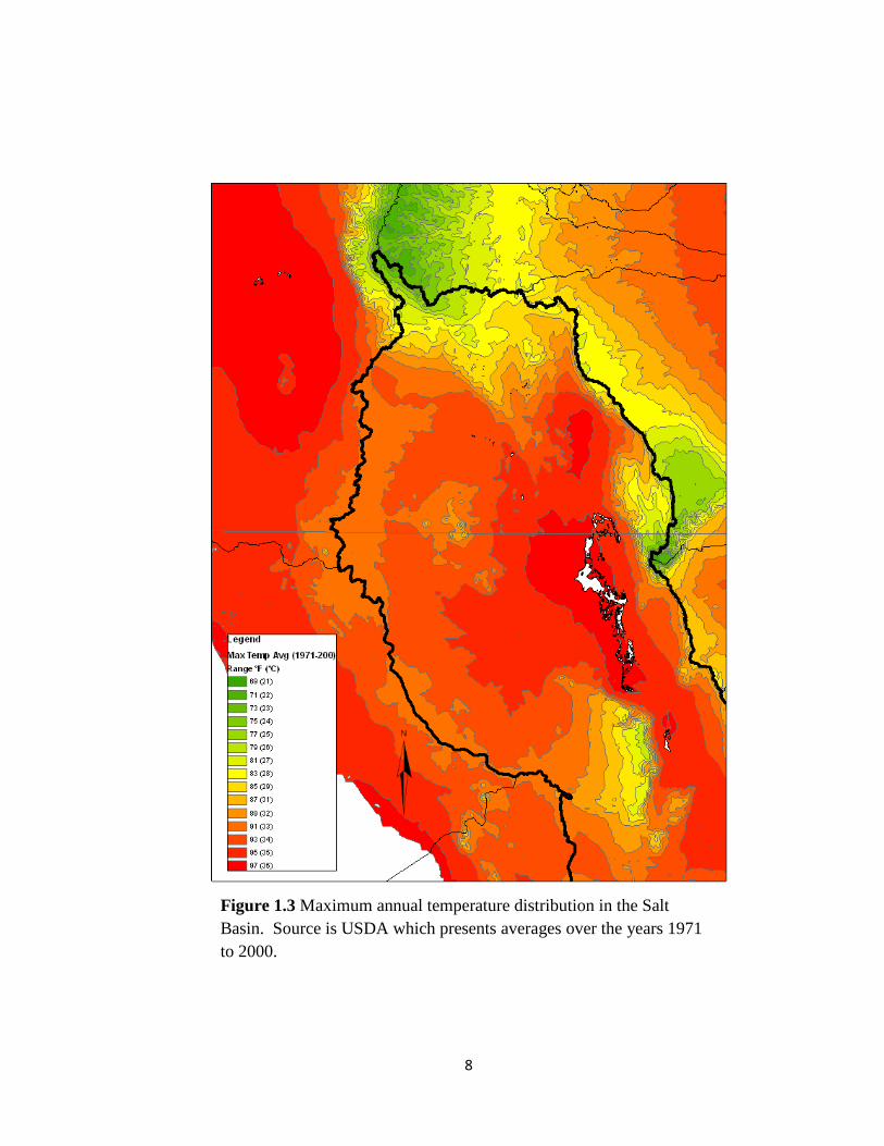
North in the Salt Basin, in the region associated with the southern Sacramento

Mountains, temperatures range from minima (fig 1.2) of -9 to -6 °C (15-20 °F) to maxima

(fig 1.3) of 21 to 23 °C (60-70 °F) with an average (fig 1.4) around 6 to 9 °C (43 to 50

°F). The lowlands in the southern Salt Basin exhibit characteristically semiarid climate

conditions. The range of temperatures throughout the year is from minima (fig 1.2) of

about -4 to 1 °C (25-33 °F), to maxima (fig 1.3) of about 29-36 °C (85-97 °F), with an

average (fig 1.4) of about 12-17 °C (53-63 °F); typically with large temperature shifts

between the day and night.

7

Figure 1.2 Minimum annual temperature distribution in the Salt

Basin. Source is USDA which presents averages over the years 1971

to 2000.

8

Figure 1.3 Maximum annual temperature distribution in the Salt

Basin. Source is USDA which presents averages over the years 1971

to 2000.

9

Figure 1.4 Average annual temperature distribution in the Salt Basin.

Source is USDA which presents averages over the years 1971 to 2000.

10

Figure 1.5 Average annual precipitation in the Salt Basin. Calculated

from averages of mean monthly precipitation using PRISM. Source is

USDA which presents averages over the years 1971 to 2000.

11

0

2

4

6

8

10

12

14

16

Jan Feb Mar Apr May Jun Jul Aug Sep Oct Nov Dec

Pre

cip

itat

ion

(cm

)

MONTH

0

5

10

15

20

25

30

35

40

45

50

Jan Feb Mar Apr May Jun Jul Aug Sep Oct Nov Dec

Sno

wfa

ll (c

m)

MONTH

(a)

(b)

Figure 1.6 Sacramento Mountains, Cloudcroft NM, monthly climate

record. (a) Average total precipitation (1914-1987) (b) Average total

snowfall (1914-1987). Western Regional Climate Center

12

The amount of rainfall received throughout the Salt Basin (fig 1.5) is quite

variable with a range from about 79 cm/yr (31 inches/yr) to about 23 cm/yr (9 inches/yr).

There is a strong correlation between precipitation and elevation as rainfall is primarily

due to orographic effects. The majority of the rainfall in the Salt Basin is associated with

the monsoon season from May to October (fig 1.6.a.). In the southern Sacramento

Mountains snowfall (fig 1.6.b) during the winter is a significant contribution to the

annual precipitation.

Section 1.2.c: Ecosystem

The ecoregions for the Salt Basin (fig 1.7) are based on the EPA‘s level IV

designation. The highest elevations with the coolest temperatures are characteristic of the

Rocky Mountain Conifer Forest ecoregion. In this region flora, fauna, and water

characteristics resemble the southern Rocky Mountains. Ponderosa pine, douglas fir, and

where it is especially cool and moist, blue spruce, are present. Typically, thick

understory is prevalent and pine needles and other organic matter litter the ground

resulting in high soil moisture. The ecosystem characteristic of the lower elevation,

southern Sacramento Mountains is the Madrean Lower Montane ecoregion, which is also

characteristic of most of the Guadalupe Mountains. In this ecoregion winters are mild

and summers are wet. Juniper and piñon pine trees are interspersed between desert

grasses.

The climate and ecoregions in the Salt Basin lowlands are a reflection of dry

semiarid conditions. There is sunshine most days of the year and mild winters that lead

to extended growing seasons. However, high temperatures and near-surface evaporation

13

Figure 1.7 Eco-Regions of the Salt Basin. Source is EPA where level

IV designations are illustrated here.

14

rates mean that irrigation is necessary for plant growth, with the exception of xerophytes

of the Chihuahuan desert vegetation. The transition from higher elevation mountains to

the Salt Basin lowlands make-up the Chihuahuan Desert Slope ecoregion. This

ecoregion extends from the southern Sacramento Mountains as disjunct hilly areas with

mixed geology that includes soil, exposed bedrock, and coarse rocky substrates.

Similarly, this ecoregion characterizes the slopes of the Guadalupe Mountains, where the

alluvial fans of rubble and sand and gravel build up at the base of the mountains.

Vegetation is mostly creosote, yucca, and prickly pear with some desert grasses. The

Chihuahuan Desert Slope grades into the Chihuahuan Desert Grasslands that encompass

the majority of the Salt Basin. Rainfall is slightly elevated in this region compared to the

Chihuahuan Basin and Playa ecoregion, generally as a result of slight heightened

elevations such as plateaus or mesas surrounding the basin lows. The Chihuahuan Basin

and Playa ecoregion represent some of the hottest and most arid in the state of New

Mexico. The sparse vegetation must be specifically adapted to withstand large seasonal

and diurnal fluctuations in temperature, low available soil moisture and high

evapotranspiration rates.

Section 1.2.d: Land and Water Use

The New Mexico portion of the Salt Basin is a sparsely populated region, where

the small communities of Timberon and Piñon, population ~300 and ~100 respectively

(U.S. Census Bureau 2000), in the southern Sacramento Mountains represent the largest

populations. Throughout the basin, southeast of the Sacramento Mountains, vast tracts of

land are privately owned, primarily by small-time cattle ranchers and sheep farmers.

These ranchers use relatively insignificant amounts of groundwater to water their

15

livestock. The western portion of the Salt Basin is largely a Military Reservation used as

a firing range where access is restricted. At the very southern extent of the New Mexico

portion of the basin, at the New Mexico, Texas state line is the Dell City Irrigation

District. This area has been heavily irrigated since the 1950‘s yielding considerable crops

of cotton and alfalfa, as well as additional crops including: peppers, melons, onions and

garlic. Over a forty year period (1950‘s-1990‘s), monitoring of the potentiometric

surface in this region shows on average a 30-40 ft drop, with a decline in water quality

over this period also observed (Sharp, 1993). This area of commercial agricultural with

irrigation by groundwater pumping represents the vast majority of the anthropogenic

groundwater discharge in the Salt Basin.

Section 1.3: Previous Work

Because of the oil and gas potential for the Salt Basin region there have been a

number of comprehensive studies addressing the structure, stratigraphy and depositional

environment for the area. King and Harder (1982) reported on the oil and gas potential of

the Tularosa Basin-Otero Platform area of Otero County, NM. Additionally the authors

published a similar report including the Salt Basin graben area for New Mexico and

Texas in 1985. These reports layout the dominant physiographic features of the Tularosa

and Salt Basin, as well as the geologic history for the region. Black‘s (1973) dissertation

on the geology of the northern and eastern parts of the Otero Platform presents

depositional and structural basin analysis. Black later published a paper in 1975 focused

on generalized structure and mechanical origins and the stratigraphy of the Otero

Platform. Broadheads‘ (2003) NM Bureau of Geology and Mineral Resources report on

the petroleum geology of the McGregor Range presents a detailed stratigraphic column,

16

and descriptions of the structure and stratigraphy of the region. Characterization of the

structure and faulting specifically for the Salt Basin graben is presented in Goetz‘s (1977)

M.S. thesis.

There have been several previous investigations into various aspects of the water

resources in the Salt Basin region. One of the earlier investigations was by Bjorklund

(1957). It focused on water levels and some general water quality observations in the

Crow Flats area. Sharp and others (1993) reported on hydrogeologic trends in the Dell

City area. This paper reported information on historic water level changes as a response

to groundwater pumping, as well as variability in water quality. Sharp and Mayer

published on the role of fractures in the regional groundwater flow in the Salt Basin in

1995. Mayer published his dissertation in 1995, also focused on fracture flow, but

included a large set of groundwater chemistry for the Salt Basin. He characterized

possible rock/water interactions responsible for the chemical trends, as well as identified

some regions of similar water chemistry within the basin. Boyd‘s (1982) Master thesis

dealt with hydrogeologic trends in the northern Salt Basin. She focused on the

geochemical trends as groundwater moved toward the salt flats from the surrounding

uplands such as the Guadalupe Mountains. Chapman‘s (1984) Master thesis built upon

Boyd‘s geochemical evolution focusing on the hydrogeochemistry and hydrodynamics at

the Salt Flats. The hydrogeology of the Diablo Plateau was characterized by Kreitler in

1990. Hydraulic characteristics of the Permian Yeso Formation were reported by

Wasiolek (1991) based on aquifer tests within the upper Rio Hondo Basin and eastern

Mescalero Apache Indian Reservation. Huff and Chace (2006) summarized reports on

the characterization of the Salt Basin groundwater system, as well as identified areas in

17

need of future investigation for resource management. In 2002 Finch published work the

hydrogeologic framework of the Salt Basin and the development of a 3-dimensional

groundwater flow model for the region. Rawling (2009), in a New Mexico Bureau of

Geology and Mineral Resources report, characterized the hydrogeology of the

Sacramento Mountains.

18

CHAPTER II

HYDROGEOLOGIC FRAMEWORK

Section 2.1: Depositional Environment and Stratigraphy

The Salt Basin is part of a larger physiogeographic province, known as the

Permian Basin. The Permian Basin formed as a consequence of the major continental

collision of the North and South American plates during the late Mississippian to early

Pennsylvanian time (Mazzullo, 1995). The onset of the Pennsylvanian Ouachita-

Marathon orogeny reactivated older, north-south to northwest-southeast oriented, basins

and uplifts (Ross, 1986; Goetz, 1985). Rapid subsidence during the Permian resulted in

extensive deposition in the platform and basin environments, which left the dominant

imprint on the geology of the Permian Basin today (Mazzullo, 1995). Subsidence ceased

at the end of the Permian. Extensive periods of erosion followed with intermittent

terrestrial and marine deposition of the Triassic and Cretaceous, respectively (Mazzullo,

1995). The block-faulting, volcanism, along with, uplift and eastward tilting of the

region that gives the basin its present structure coincided with the Laramide orogeny

starting in the late Cretaceous (Mazzullo, 1995).

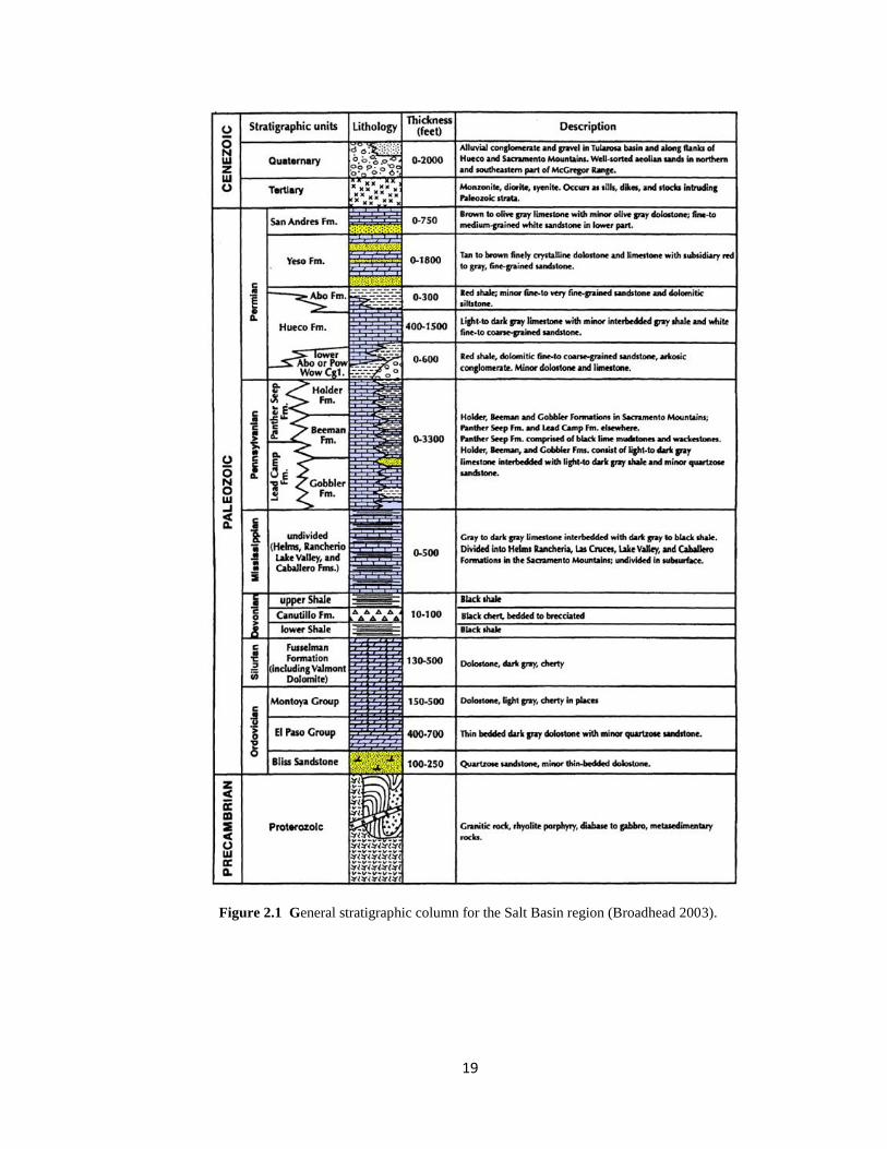
Broadhead (2003) presents a stratigraphic column for the region spanning the

Precambrian to the end of the Cenozoic (fig 2.1). Based on the work of King (1982), the

oldest known Precambrain bedrock in the Salt Basin region is 1.35 Ga, Chaves Granitic

19

Figure 2.1 General stratigraphic column for the Salt Basin region (Broadhead 2003).

20

Terrane across which later Precambrain sediments were deposited. These later sediments

were eventually metamorphosed and underwent subsequent igneous intrusions. The

Precambrain formations may have undergone further alteration from additional episodes

of burial and uplift until eventually the area was deeply eroded to a surface over which

the lower Paleozoic rocks were deposited (King 1982). The Cambrian-Ordovician seas

spread throughout the region depositing the basal arkosic Bliss Sandstone. King (1983)

describes this sequence followed by Ordovician and Silurian carbonate deposition of the

El Paso, the Montoya, and the Fusselman Formations. While rocks older than the

Permian are rarely considered significant contributors of water within the region, the

Silurian Fusselman dolomite has been reported by the oil and gas exploration industry as

having ―fresh water‖ in the Otero Mesa/Diablo Plateau areas (Finch, 2002). This

formation is generally found at depths greater than 2,000 ft below the land surface

(Black, 1975).

By the Devonian the region was predominantly a shallow sea where dark organic

deposits of mud and silt formed (King, 1982). In the Mississipian the sea levels had

advanced leaving a variety of carbonate deposits. However, within the region the

Mississipian rock are mostly missing due to erosion during the Pennsylvanian (Black,

1973). By the middle of the Pennsylvanian the Pedernal uplift became a dominant

structural feature in the region. The southern extension of this positive feature and the

subsequent formations of lowlands on either side played a significant role in the

deposition of the middle to late Pennsylvanian sediments (King, 1982). King interprets

one of the primary results of this uplift to be the transition from the Hueco Formation of

21

calcareous marine facies into the terrestrial redbed facies of the later Abo Formation. By

the Wolfcampian all of the Pedernal was buried beneath the Abo redbeds (Black, 1973).

The Permian limestone of the San Andres and Yeso are the dominant stratigraphic

outcrops covering much of the extent of the Salt Basin (fig 2.2). The Yeso Formation of

interbedded gypsum, dolomitic calcareous mud, and pinkish silt mud was deposited

inland over the Abo Formation (King, 1982). The Yeso is a very heterogeneous

stratigraphic unit, ultimately composed of sandstone, limestone, dolomite, siltstone, shale

and evaporites. In later deposits the Yeso sediments slightly interfinger with the San

Andres deposition, which often makes distinguishing the contact difficult (King, 1982).

The Yeso and the San Andres Formations are the uppermost stratigraphic units and are

believed to be deposited throughout the Leonardian to the Guadalupian (King, 1982).

Dolomite is prevalent throughout the San Andres Formation (Wasiolek 1991). The

conditions necessary for seawater to evaporate to the extent of dolomitizing calcite are

characteristic of a supratidal flat environment. This is where the shore level is

immediately marginal to and slightly above the high tide level (Milner 1976).

Depositional facies in the Yeso and San Andres units show successions of low-stand sea

level conditions where aqueous or subaqueous sandstones are preceded by high-stand

conditions under which limestone and dolomites are deposited (Broadhead, 2003).

Following the final gypsum deposits of the upper San Andres Formation the Permian seas

retreated, upon which exposure led to dissolution of gypsum and limestone in the San

Andres Formation creating a karst environment (King, 1982).

The Tertiary, now only classified as the Paleogene to the Neogene (Gibbard,

2009), can be characterized by the onset of igneous activity. The most significant

22

Figure 2.2 Surface geology of the northern Salt Basin. Geology from Stoeser et al.

(2005), with location of alkali flats/playa lakes for New Mexico taken from NHD.

23

igneous features in the Salt Basin are the Cornudas Mountain intrusions, which are

exposed laccoliths and sills predominantly syenite in composition (King, 1982). The

Pleistocene marks a time of predominant erosion with some Holocene lake-bed deposits

forming in the small, closed basin and playas between the uplifts (Black, 1973). Black

also discussed terracing, slumping and solution collapse during the Holocene, along with

alluvial fan, arroyo and streambed deposition. Due to the nature of its origin, the

alluvium is primarily composed of broken-up limestone, which can be clearly observed in

the field.

Section 2.2: Structure

King (1982) discussed the general structure of the Salt Basin in relation to

different periods of deformation from the Pennsylvanian to the Neogene. He attributes

most of the primary folding and faulting at crests of anticlines to deformation during the

uplift of the Pedernal landmass in the late Pennsylvanian time. The buried Pedernal

landmass (fig 2.3) is a north-south trending feature which is structurally dominant in

Otero Mesa (Black, 1975). The buried Pedernal uplift is also of importance in how rock

yielded later during the Laramide deformation. During east-west compression the uplift

may have acted as a buttress against which the Otero folds were pushed. Rocks overlying

the Pedernal and the areas to the east of the feature were less deformed.

Mid- to late- Permian structural features include: the Otero fault, Bitterwell

Break, Babb and Victorio flexures (fig 2.3). The Babb and Victorio flexures are

northeast-southeast trending monoclines with a northeastward dip (King, 1948). The

Babb flexure and the more easterly-trending Victorio flexure cut through the basement

24

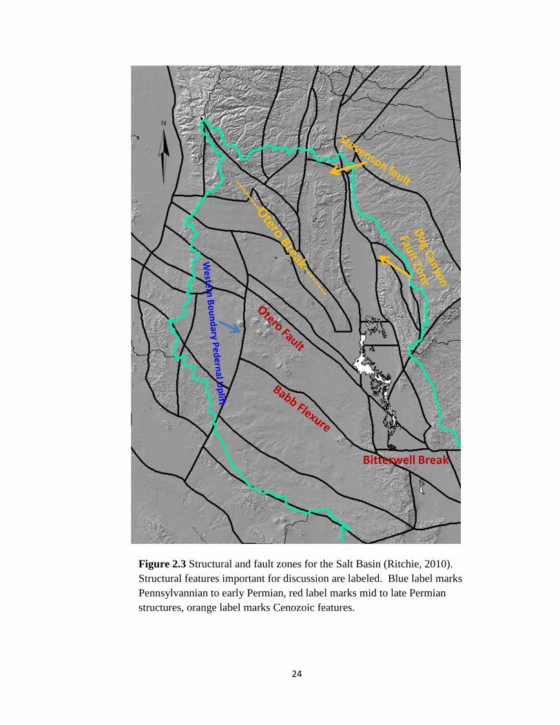
Figure 2.3 Structural and fault zones for the Salt Basin (Ritchie, 2010).

Structural features important for discussion are labeled. Blue label marks

Pennsylvannian to early Permian, red label marks mid to late Permian

structures, orange label marks Cenozoic features.

25

blocks of the Salt Basin graben, and intersect on the east side of the graben (Goetz,

1980). Both flexures are ringed by reefs of Leonardian age (King, 1948). The Otero

fault is a northwest-striking fault with displacement down to the northeast (Goetz, 1985).

The fault cuts through Otero Mesa and continues southeast towards Dell City along the

northeast side of the Cornudas Mountains (Goetz, 1985). The Bitterwell Break is a fault

in the basement blocks of the Salt Basin graben that trends east-west from the Babb

Flexure to the Delaware Mountains (Goetz, 1985). The trend corresponds to the northern

boundary of the Sierra Diablo where the down-to-the-north displacement (Goetz,1980)

results in a groundwater divide for the northern portion of the Salt Basin (Sharp, 1985).

Subsequent Laramide deformation during the late Cretaceous created many of the

northwest and north trending folds that are relatively symmetrical, gently dipping and

commonly double plunging (King, 1982). These include the Otero and Cornucopia folds

as well as possibly the Jernigan wash anticline, and subtle Chert Plateau folds (Black,

1975). High-angle normal faults are common along the crest and steep west flanks of

major anticlines in the Salt Basin (fig 2.4). In addition to the faults associated with the

anticlines, north-trending high-angle normal faults of the Cornucopia Hills (fig 2.4) likely

underlie the alluvial cover in both Cornucopia Draw and Jernigan Wash (Black, 1975).

Neogene tectonics associated with basin-and-range provinces has resulted in a

series of tilted fault blocks, each progressively less deformed and uplifted to the south

and east, that characterize the present structure (King, 1982). The Guadalupe fault zone

and its possible westward extension known as the Stevenson fault that bounds the

northeast and east edges of the Salt Basin are some of the most prominent Cenozoic

structures (fig 2.3). The imposing west-facing escarpment of the Guadalupe Mountains is

26

Figure 2.4 Tectonic structural features of the Salt Basin during the Cenozoic (Goetz,

1986, Black, 1975)

27

a result of the closely spaced high-angle normal fault zone where the alluvium meets the

foot of the Guadalupe rim (Black, 1975). The Sacramento and Orendorf anticlines and

intervening Sacramento River and Otero syncline, McGregor anticline, Prather anticline

and syncline are all primarily caused by drapefolding over deep-seated fault blocks which

have been gently titled to the northeast (Black, 1975). West-oriented extension during

the Neogene turned these into a series of west dipping normal faults (fig 2.4) extending

northwest to southeast from the Sacramento Mountains, known as the Otero Break

(Goetz, 1985; Mayer, 1995).

28

CHAPTER III

WATER RESOURCES

Section 3.1: Surface Water

The major watersheds within the Salt Basin are the Sacramento River and Piñon

Creek. The Sacramento River (fig 3.1), which originates in the Sacramento Mountains, is

the only perennial surface water in the basin. The flow is perennial only on relatively

limited distances of the river before infiltrating to the shallow groundwater (Rawling,

2009). The headwaters of these perennial reaches are commonly associated with minor

wetlands, also present around springs in the Sacramento Mountains. Wetlands are likely

to be sites of groundwater recharge as they are permanently saturated, indicating

hydraulic connectivity with the shallow water table in the region. The locations, flow

directions and interactions with groundwater of the Sacramento River and other

headwaters within the Sacramento Mountains are influenced by the structural features of

the region. Uplift of the Sacramento Mountains produced an eastward dip of both the

geologic layers and the topographic surface (Rawling, 2009). Intersection of this surface

with the down-faulted western edge of the range created a crest that forms a drainage

divide between streams flowing to the east in the Pecos River and drainage to the west to

the Tularosa Basin. The Sacramento River is an exception as it flows southeast into the

Salt Basin graben. Near the headwaters the daily mean stream flow of the Sacramento

River ranges from 2-13 cubic feet per second (USGS database). With increasing distance

29

from the headwaters the ephemeral reaches of the Sacramento River diffuse out to join

the lower channel networks present in the Salt Basin.

Significant ephemeral flow channels throughout the Salt Basin (fig 3.1) include

Piñon Creek, Cornucopia Draw, Big Dog Canyon, and Shiloh Draw. A recent USGS

investigation based on channel geometry, reported estimates (table 3.1) for the annual

flow and infiltration contribution to the Salt Basin from the major channel networks. For

the Sacramento River, Piñon Creek, Cornucopia Draw, Big Dog Canyon an estimated

total of about 60,000 acre-ft of annual flow with between 27 to 56 percent loss by

infiltration was reported (Tillery, 2010).

Subbasin

Maximum annual-flow estimate, in

acre-ft

Most downstream annual flow

estimate, in acre-ft

Difference between maximum annual flow and downstream

annual flow, in acre-ft

Flow loss, in percent

Stream miles over which losses occur

Sacramento River 10,866 6,013 4,853 45 16.0

Cornucopia Draw 15,212 6,737 8,475 56 16.4

Piñon Creek 29,700 21,723 7,977 27 9.2 Big Dog Canyon 4,636 2,970 1,666 36 6.1

Table 3.1 Flow losses and associated distances for the four major subbasins studied in the

Salt Basin (USGS; Tillery, 2010)

30

Figure 3.1 Salt Basin sub-watersheds. Modified from Huff and

Chace (2006).

31

Section 3.2: Groundwater Aquifer System

The carbonate formations of the Permian are attributed as the major aquifers

within the Salt Basin. These are primarily carbonate and mixed carbonate/evaporite

sequences formed in shelf-margin to basinal marine depositional environments

(Mazzullo, 1995). In the New Mexico portion of the Salt Basin the significant Permian

carbonate aquifer is formed by the San Andres and Yeso Formations (Huff and Chace,

2006). Some previous work on developing groundwater flow models of the Salt Basin

suggested that these Permian carbonates act as a single hydraulic unit (Mayer, 1995).

The eastern reef formations of the Guadalupe Mountains were recognized as a possible

exception to this interconnectivity. The vertical connectivity of the deeper, possible

aquifer units of the Hueco and the Abo formations, with the primary aquifer is also

unknown.

Section 3.2.a: Hydrostratigraphic Units

-Abo and Hueco Formations

Typically groundwater wells do not penetrate past the Yeso formation so the

hydraulic characteristics of the Abo and Hueco formations are poorly known. However,

some outcrops of the formations in New Mexico are said to be a source for wells (Huff

and Chace, 2006). Based on stratigraphy, the Abo can be separated into three distinct

sequences, described by Black (1975). The lower Abo is conglomerate redbed. The

middle sequence is known as the Hueco, which thickens to the south and is a dark-gray,

fine grained, thin to medium-bedded fossiliferous limestone. The upper Abo sequence

32

consists of reddish-brown mudstone, fine-grained sandstone and siltstone, with a

southward-thickening tongue of gray shale, limestone and dolomite (King, 1982).

-Yeso Formation

The Yeso Formation is composed of a variety of lithologic types including

limestone and dolomite; red, yellow and gray shales and siltstones; evaporites, primarily

gypsum/anhydrite and minor halite; and yellow, fine-grained sandstone (Black, 1975).

The Yeso was deposited on the Abo where the contact is defined by the presence of

gypsum or lowest pinkish clastic bed (Black, 1975). The formation is approximately

1,000 feet thick, the lower 500 ft is associated with more evaporites and siltstones (Kelly,

1971). This depositional trend means that most well that produce water from the Yeso

Formation penetrate the upper 500 ft in the fractured limestone and dolomite where the

permeability is higher due to dissolution and fractures. In the southern reaches of the

Sacramento Mountains wells drilled in the lower Yeso Formation generally yield less

than 5 gallons per minute (gpm) while wells in the upper portion of the formation have

yields greater than 20 gpm (Finch, 2002). Wasiolek (1991) reported that the hydraulic

conductivity determined by deep aquifer tests on Yeso formation under the Mescalero

Apache Indian Reservation averaged 7.0 x 10-8

m/s (0.02 ft/d) for unfractured siltstone

and gypsum beds. The average hydraulic conductivity for the Yeso formation, where

flow is preferentially through fractures and dissolved limestone beds, ranged from 2.1 x

10-6

to 5.3 x 10-6

m/sec (0.6 to 1.5 ft/d). This indicates that, for the Yeso formation in this

region, limestone beds with secondary permeability have orders of magnitude higher

hydraulic conductivities than those of unfractured beds (Wasiolek, 1991).

33

-San Andres Formation

Like the Yeso Formation, water movement through the San Andres Formation is

largely facilitated through fracture flow and dissolution channels in the

limestone/dolomite bedding. The lower contact of the San Andres is formed by

gradational interfingering of Yeso and San Andres carbonate rocks (Black, 1975). The

interfingering can make distinguishing between the two units difficult. The San Andres

Formation is primarily light-olive-gray dolomite and dolomite limestone with sandstone

and shale lenses. The San Andres carbonates are highly jointed meaning, fractures are

slightly displaced perpendicular to the fracture surface and not in any other direction

(Rawling, 2009). The bedding of the formation is quite variable, with bedding thickness

commonly between 2-5 feet, while massive bedding can sometimes be as great as 20 feet.

Sharp and Mayer (1995) quantified estimates of the extent of the preferential flow

through fractures zones using a basin scale flow model for the Salt Basin. The flow

model generated the best fit of the potentiometric surface in the Salt Basin assuming an

average hydraulic conductivity of 10-4

m/s within fracture zones and an average of

10-6

m/s outside the fracture zones. Groundwater flow through fractures was also

attributed with significant differences in well production during the development phases

of Dell City. In the drilling of irrigation wells it was observed that approximately 50

percent of the wells drilled were high yield (>1000 gpm) while the other half were

relatively low yield (<500 gpm), even in very close vicinity, as close as 100 ft (Scalopino,

1950). In general, the aquifer in the Dell City region is a considered to have high

transmissivity. Kreitler (1990) observed that extensive groundwater production,

34

approximately 108 m

3/yr (98,500 acre-ft/yr) pumped for irrigation for 30 years, resulted

in only 10 m (33 ft) of drawdown.

- Cretaceous Limestone

In the Diablo Plateau, Cretaceous limestone is considered part of the aquifer, in

addition to the Permian aquifer system. These sequences are characterized by yellowish-

tan to light-gray nodular, fossiliferous limestone and brownish-tan to orangish-tan

sandstone and siltstone. Like the Permian aquifer system in the Dell City area, the

Cretaceous limestone aquifer across the Diablo Plateau is also considered to have high

transmissivity. Kreitler (1990) reported the hydraulic gradient for the Diablo Plateau

aquifer as approximately 1m/km (5 ft/mi), which is relatively low considering the 400 m

(1,300 ft) of relief.

Section 3.2.b: Source, Occurrence and Movement of Groundwater

The northern portion of the Salt Basin is a hydrologically closed basin with about

12,000 km2 of surface area drainage. The Sacramento Mountains to the north of the

basin constitute a high mountain environment that is a significant source of recharge to

the Salt Basin. Winter snowfall (fig 1.6.b) that infiltrates into the spring/stream systems

is the dominant source of recharge to the regional aquifer system during average

precipitation years (Rawling, 2009). The streams distribute the recharge over a larger

area than the winter snow pack (Rawling, 2009). Thus, one of the most significant

sources of recharge to the aquifer system underlying the Salt Basin is likely infiltration of

stream flow from the Sacramento River and Piñon Creek watersheds (fig 3.1) which

originate in the Sacramento Mountains (Finch, 2002; Mayer, 1995; Sharp, 1993). The

35

infiltration can take place directly within the Salt Basin watershed or act as a source of

recharge as an underflow flux across the northern surface-water divide from the

Sacramento Mountains.

Precipitation falling anywhere within the Salt Basin surface water divide can

infiltrate to the groundwater system as long as precipitation and infiltration rate exceed

the rate of evaporation. However, across most of the Salt Basin precipitation is so low

and evaporation rates so high that only high intensity storm events have the potential for

recharge. Canyon systems and ephermal drainage networks off the steep western face of

the Guadalupe Mountains focus runoff to the bajadas. The bajadas are a sequence of

alluvial fans spreading onto the Salt Basin floor where the shallow slopes and coarser

grained material facilitate recharge to the aquifer system. Otero Mesa and Diablo Plateau

are also sources of recharge to the Salt Basin. Recharge is thought to infiltrate over the

entire plateau ~approximately 7,500 km2

(Mullican, 1987; Kreitler, 1990). The recharge

infiltrates through fractures along arroyos during storm events and flooding, rapidly

entering the aquifer system. Ephermal watercourses such as Eightmile Draw, drain the

majority of the Diablo Plateau where dendritic drainage networks converge to enter the

Salt Flats 15 km south of Dell City (Goetz, 1977). Historic flood events can result in

standing surface water on the Salt Flats (Chapman, 1984).

The regional groundwater flow (fig 3.2) is south-southeastward from the recharge

area of the Sacramento Mountains and eastward from the Otero Mesa/Diablo Plateau

toward the Salt Basin graben and Dell Valley (Mayer, 1995; Sharp, 1993). Groundwater

flows from the Sacramento Mountains into the Dell Valley area to the Salt Flats through

a set of northwest-southeast trending fractures (Mayer and Sharp, 1995). Groundwater

36

flow from the Otero Mesa generally follows the structural dip which is gently east-

sloping toward the Salt Basin graben (Mayer, 1995; Kreitler, 1990). The groundwater

divide is close to the southern edge of the Diablo Plateau from which groundwater flows

southwest to northeast. Like the Otero Mesa this groundwater is thought to flow down

the structural dip of the monocline, with only a minor amount flowing south-westward

into Hueco Bolson (Kreitler and Mullican, 1990). Water entering the northern portion of

Salt Basin graben is hydrologically isolated from the extension of the southern Salt Basin

graben by the Bitterwell Break (fig 3.2). This is a Neogene normal fault that deforms the

sediments of the Salt Basin and produces a groundwater divide (Sharp, 1985; Boyd,

1986). This southern boundary extends west to the Babb flexure, a northwest-southeast

trending, north-side-down monocline, as previously discussed. The Salt Flats (fig 3.2)

are a series of gypsum playas along the eastern margin of the Salt Basin graben that

constitutes the natural discharge point for this closed basin (Chapman, 1984; Boyd,

1982). However irrigation near Dell City began around 1950‘s and has since been a

significant amount of the groundwater discharge (Sharp and Mayer, 1993).

37

Figure 3.2 Groundwater movement and groundwater elevation contours

(ft). Groundwater contours taken from (Ritchie, 2010).

38

CHAPTER IV

METHODS AND ANALYTICAL TECHNIQUES

Section 4.1: Groundwater Chemistry Dataset

To obtain a better spatial distribution of the groundwater chemistry in the Salt

Basin, data collected specifically for this study of the Salt Basin were supplemented with

data obtained from previous studies (fig 4.1). Supplementary data were obtained from

two main sources: spring and well samples from the Sacramento Mountains collected by

the New Mexico Bureau of Geology and a general chemistry dataset from wells

throughout the Salt Basin compiled by Mayer for his 1995 dissertation. Specifics of

sample collection and analysis are discussed below for each data source.

Section 4.2: Current Salt Basin Study

Twenty five water chemistry samples from groundwater in the Salt Basin were

collected during a series of field trips in 2008—2009 (fig 4.2). Wells were sampled

along regional flow paths (fig 3.2), east of the Otero Break, starting in the southern

Sacramento Mountains and ending near Dell City and the Salt Flats. Samples from these

sites were analyzed for a wide variety of constituents: major- and minor-element

chemistry, oxygen-18 (18

O) and deuterium (D) content, carbon-13 (13

C) and

carbon-14 (13

C) content of dissolved inorganic carbon, sulfur-34 (34

SO4) content of

dissolved sulfate, and tritium (3H). Water analyses are tabulated in table 5.1 and

Appendix A.

39

Groundwater sampling sites for the Salt Basin study were selected primarily on

the basis of location in an attempt to attain the most comprehensive geochemical

evolution along the given flow paths. Choice of sampling sites was limited primarily due

to access issues. For example, private land owners denied permission to take a water

sample, or in the case of most of the western side of the Salt Basin access is limited due

to the military reservation, as previously discussed.

Of the 25 wells that were sampled, 4 were domestic wells (wells used to supply

water to fewer than 3 households), 3 were irrigation wells (wells used for commercial

agricultural production), 2 were powered by windmills (wells having a piston mechanism

to lift water, which is used primarily to water stock), 3 were powered by solar panels

(wells where solar panels powered submersible pump, which is used primarily to water

stock), 1 well was spring fed (shallow well directly drilled into a spring), and 12 were

classified as other (wells with submersible pumps, where water is used primarily to water

stock). Well depths ranged from about 60 to 1600 ft, with an average of about 630 ft.

Information on well depth, depth to water and screened interval was obtained from the

landowner and was often limited or approximate. Sampling site locations (fig 4.2) were

taken using a Garmin 60 GPS unit.

Section 4.2.a: Collection of Groundwater Chemistry

Purging the well insures that water samples collected are not from water stored

in the well bore volume. Ideally, if the column depth and well casing radius were known

the well bore volume could be calculated and at least 2 well bore volumes were

discharged and field parameters (specific conductance, water temperature, pH, and

dissolved-oxygen concentration) were allowed to stabilize before sample collection. If

40

there was limited information on the well, the wells were pumped in such a way that

discharge could be collected in buckets and measurements were taken until field

parameters had stable readings over a significant volume of water. Generally, some

estimate for bore volume could be made. The general chemistry water samples were

collected in 250 ml nalgene polyethylene bottles. For trace metals 125 ml of water was

collected which needed to be filtered (0.45 micron filters) and kept on ice with the

general chemistry samples until delivered for analysis. The oxygen (18

O) and

hydrogen isotope (D) samples were collected in small (~25 ml) glass vials, underwater

to prevent contact with the atmosphere. There should not be air bubbles present in the

collected samples and freezing and sun exposure were avoided. For the sulfur isotopes

(34

SO4) measured from sulfate in the groundwater; two 500 ml nalgene polyethylene

bottles were collected. Groundwater samples for tritium (3H) content were collected in

two 500 ml nalgene polyethylene bottles that were filled, underwater to prevent

contamination. It was critical to remove wristwatches where glow in the dark dials can

have traces of tritium that can contaminate the sample. The carbon-14 (14

C) and

carbon-13 (13

C) samples were collected in a 1 liter nalgene polyethylene bottle. To

prevent contamination of the sample in this case, it was very important that gloves be

worn during the collection. In every case the sample bottles and caps were rinsed 2-3

time in well water before collection of the actual sample.

Section 4.2.b: Precipitation Collection

In addition to groundwater samples, four precipitation collectors were set-up

throughout the eastern side of the Salt Basin and analyzed for stable isotopes of oxygen-

41

18 (18

O) and deuterium (D). Precipitation collectors employed are referred to as PVC

collectors (Earman, 2006). The PVC (polyvinyl chloride) collector consists of a 19-cm-

diameter plastic pipe, approximately 1.25 m high, sealed at the bottom, and mounted to a

stake about 1 m off the ground, with a layer of mineral oil in the bottom of the collector.

The mineral oil prevents evaporation of the precipitation in the collector. The

precipitation collectors were placed in the open, away from trees or structures that might

prevent interference. The precipitation was collected seasonally to be analyzed for the

stable isotope content.

Section 4.2.c: Analytical Techniques

General chemistry

Analysis of major- and minor elements for the Salt Basin study was performed by

the New Mexico Bureau of Geology and Mineral Resources Chemistry (and water quality

analysis) Lab. Water chemistry was analyzed using the United States Environmental

Protection Agency (USEPA) Clean Water Act Analytical Methods (USEPA, 2010). The

analyses include conductivity, alkalinity, pH, total dissolved solids (TDS), hardness,

bromide, chloride, fluoride, nitrate, nitrite, phosphate, sulfate, sodium, potassium,

magnesium, and calcium. Conductivity was calculated according to USEPA method

120.1, Conductance and Specific Conductance. The pH was calculated according to

USEPA method 150.2, pH, Electrometric (Continuous Monitoring). The TDS was

calculated using Standard Methods for the Examination of Water and Water Quality

(1992). The alkalinity was determined according to USEPA method 310.2, Alkalinity,

Colorimetric, Automated Methyl Orange. Analyses of major cations were performed

42

according to USEPA method 200.7, Determination of Metals and Trace Elements in

Water and Wastes by Inductively Coupled Plasma-Atomic Emission Spectrometry

Revison 4.4. The inorganic anion chemistry was determined according to USEPA

method 300.0, Determination of Inorganic Anions by Ion Chromatography. Reporting

limits with methods for conductivity and TDS are 10 S/cm and 10 mg/L, respectively.

Anion reporting limits are the typically 1 mg/L (with the exception of bromide 0.1 mg/L,

or for low bromide 0.001 mg/L). Cation reporting limits are 0.001 mg/L.

Trace metals

Analyses of trace metals were performed by the New Mexico Bureau of Geology

and Mineral Resources Chemistry (and water quality analysis) Lab. Trace metal analyses

included aluminum, antimony, arsenic, barium, beryllium, boron, cadmium, chromium,

cobalt, copper, iron, lead, lithium, manganese, molybdenum, nickel, selenium, silica,

silicone, sliver, strontium, thallium, thorium, tin, titanium, uranium, vanadium, and zinc.

Trace metals were analyzed using the United States Environmental Protection Agency

(USEPA) Clean Water Act Analytical Methods (USEPA, 2010). Specifically, trace metal

content was determined by USEPA method 200.8, Determination of Trace Elements in

Water and Wastes by Inductively Coupled Plasma-Mass Spectrometry Revision 5.4. For

this method the reporting limits are typically 0.001 mg/L.

Oxygen (18

O) and hydrogen (D) isotopes

Analysis of the oxygen (18

O) and deuterium (D) stable isotope content for the

groundwater and the precipitation samples were performed by New Mexico Tech Stable

Isotope Laboratory which is directed by Andy Campbell. The 18

O content of a 1 mL

43

water sample was determined using the CO2/H2O equilibration method as described in

Clark and Fritz (1997). The samples react in sealed containers, from which the

equilibrated CO2 gas is extracted into the Thermo Finnigan Gasbench operated in

continuous flow mode. The D content of the water sample is analyzed from hydrogen

gas generated by metal reduction with powdered chromium at 850 °C in an H-Device

(Nelson and Dettman, 2001). The gas entry to the mass spectrometer is regulated by a

dual inlet system such that the hydrogen gas from the H-device is stored in a bellows, and

run against and standard hydrogen gas stored in another bellows. Both the CO2 and H2

were analyzed on a Thermo Finnigan DeltaPLUS

XP Stable Isotope Ratio Mass

Spectrometer. The stable isotope results are reported with respect to Vienna Standard

Mean Ocean Water (VSMOW). The delta value is given by

, where

R is the ratio of the heavy to the light isotope measured from counts by the mass

spectrometer (Sharp, 2007).

34

S in SO4

The analyses of the 34

S stable isotope content of sulfate from the groundwater

samples were performed by the New Mexico Tech Stable Isotope Lab. Sample

preparation is performed according to the United States Geological Survey (USGS)

Determination of the (34

S/32

S) of sulfate in Water: RSIL Lab Code 1951. The dissolved

sulfate from the groundwater sample is precipitated with barium chloride (BaCL2) to

barium sulfate (BaSO4). The Elemental Analyzer (EA) is used to convert sulfur in the

BaSO4 sample precipitate into SO2 gas. The EA introduces the SO2 gas through

continuous flow connected to the Thermo Finnigan DeltaPLUS

XP Stable Isotope Ratio

44

Mass Spectrometer which determines the sulfur isotope ratio. 34

S values are reported

relative to the Cañon Diablo Troilite (CDT) standard. The delta value is given by

, where R is the ratio of the heavy to the light isotope measured from

counts by the mass spectrometer (Sharp, 2007).

3H Tritium

The tritium (3H) analysis was performed by University of Utah Gas Lab. The

tritium content of the groundwater samples was determined by helium ingrowth methods.

The method begins by degassing the water sample under high-vacuum to extract the

dissolved gases. The sample is sealed and sits for 6 to 12 weeks while tritium decays and

helium-3 grows. After the sample is decayed, the levels of helium-3, which directly

correlate to the amount of tritium decayed, is measured using Mass Analyzers Products-

Model 215-50 Magnetic Sector Mass Spectrometer. The system setup and analysis

process is designed based on the design described in A static Mass Spectrometer with

Triple Collection for Nitrogen and Neon Samples, Scripps Oceanographic Institute, S.I.O

Reference series #93-11 (1993). The results are reported in tritium units (TU); in water

of 1 TU the specific activity is equal to 3.2 picocuries per liter (pCi/L), or 7.1

disintegration per minute per liter (dpm L).

Carbon-14 (14

C) and Carbon-13 (13

C)

The carbon-14 (14

C) and carbon-13 (13

C) content of the groundwater samples

were determined by Beta Analytic Incorporated. The radiocarbon dating was performed

using accelerator mass spectrometry (AMS) counting. First, the dissolved inorganic

carbon (DIC) was precipitated as strontium carbonate (SrCO3) using strontium chloride

45

(SrCl2). This was rinsed to a neutral solution and dried. The precipitate was then

acidified using 0.5 N H3PO4 phosphoric acid and the carbon was collected as CO2 gas.

The gas is then mixed with hydrogen over a cobalt catalyst and heated to 600 °C reducing

the carbon to graphite on the cobalt. The graphite is the analyzed by an AMS and

measured for the carbon isotope content. By international convention, the modern

reference standard was 95% the 14

C activity of the National Institute of Standards and

Technology (NIST) Oxalic Acid (SRM 4990C).

46

Figure 4.1 Salt Basin well sample locations. Grid coordinates are in

Northing (m) and Easting (m). The water elevations contours are from

Richie (2010) refer to figure 3.2.

47

Section 4.3: NMBGMR Sacramento Mountain Study Groundwater Chemistry

The New Mexico Bureau of Geology and Mineral Resources is involved with an

ongoing study of the hydrogeology of the Sacramento Mountains in southern New

Mexico. The goals of the study are to delineate areas of groundwater recharge, determine

directions and rates of groundwater movement, and to characterize the interactions

between different aquifers and groundwater and surface-water systems. In the study a

variety of techniques are utilized to characterize the regional hydrogeology including

water chemistry analyses, isotopic analyses, and groundwater age dating. The dataset for

the Sacramento Mountains Hydrogeology Study open file report-518 (2009) is available

to the public. The preliminary interpretations and dataset from the study was draw on for

this Salt Basin study in defining the recharge area of the Sacramento Mountains.

Specifically, groundwater chemistry from wells within delineated zones of modernly

recharging groundwater were used as initial points in flow paths for geochemical

modeling. The database includes latitude and longitude for each sample site (fig 4.1).

Samples that did not include at least major- and minor element chemistry were not

included in the Salt Basin analysis. The constituents of the chemical analyses from the

NMBGMR study (reference numbers are preceded by ―SM‖) are listed in table 5.1 and

Appendix B: major- and minor-element chemistry, oxygen-18 (18

O) and deuterium

(D) content, carbon-13 (13

C) and carbon-14 (13

C) content of dissolved inorganic

carbon, and tritium (3H). The analytical techniques for the chemical analyses for the

water samples are likely similar to those described in sections 4.2.a and 4.2.c as

procedures for the Salt Basin study were modeled after procedures of the NMBGMR.

48

Section 4.4: Groundwater Chemistry Dataset Compiled by Mayer (1995)

For Mayer‘s (1995) dissertation on The Role of Fractures in Regional

Groundwater Flow in the Salt Basin, he compiled a comprehensive dataset of the

regional groundwater chemistry. Mayer sampled about 35 well sites throughout the Salt

Basin and analyzed them for pH, temperature, alkalinity, conductivity, and the

concentration of selected ions (Ca2+

, Mg2+

, Na+, K

+, F

-, Sr

2+, Cl

-, Br

-, SO4

2-, NO3

2-). The

analytical techniques for the water analyses are described in his thesis (Mayer, 1995). He

supplemented his work by compiling regional groundwater chemistry from published

reports and government records. Sources of chemical data used in his study included

Kreitler et al. (1987), Ashworth (1994), and the Texas Water Development Board for the

Dell Valley and Diablo Plateau regions; Bjorklund (1957) from the New Mexico State

Engineer‘s Office, and Hudson and Borton (1980) for Crow Flats; and the U.S.

Department of the Interior, Bureau of Land Management for wells on federal lands in

New Mexico. Mayer discusses the potential complications in using data from different

time periods. He makes three main assumptions: (1) apart from irrigated areas (where

only predevelopment water chemistry was included) water chemistry has remained

constant through time, (2) bias from older analytical techniques are negligible because

water analyses are high in total dissolved solids and major constituents are above the

detection limits, and finally (3) that pre-1950 pH analyses are likely not reliable as

measurement techniques are unknown. For my study, the dataset Mayer (1995) compiled

was only used to assess the regional distribution of pertinent ion chemistry and was not

used quantitatively for any of the geochemical modeling.

49

For the maps present in his dissertation Mayer determined well positions from

U.S. Geological Survey 7.5 minute topographic maps. Other than his maps of the well

locations within in the Salt Basin he did not provide coordinates. To determine latitude

and longitude positions for his well locations, I geo-referenced his maps using arcGIS

and matched up well locations (fig 4.1) to wells from NWIS database. A few wells did

not correspond to wells from the NWIS database and were assigned approximate

positions; these exceptions are specified in the data table. Site locations, water analyses,

and the source for the well chemistry are listed in Appendix C.

50

Figure 4.2 Distribution of comprehensive well water chemistry dataset used for

analysis for the Salt Basin. Digital Elevation Map (DEM) provided by the USGS

National Elevation Dataset. Water elevation contours are from Ritchie (2010) refer

to figure 3.2

51

CHAPTER V

INTERPRETATION OF ENVIRONMENTAL TRACERS IN GROUNDWATER

Section 5.1: Ion Chemistry as Subsurface Tracers

Specific processes within the hydrologic cycle affect the transport and reactions

involving the ion chemistry of natural waters. Fluxes of solutes from rainfall and runoff

as well as chemical reactions within the soil and saturated zone operate to increase or

decrease the abundance of dissolved constituents in water. For most groundwater, 95%

of the ions are represented by 8 major ionic species (Herczeg and Edmunds, 2000). The

positively charged cations include sodium (Na+), potassium (K

+), calcium (Ca

2+) and

magnesium (Mg2+

) and the negatively charged anions include chloride (Cl-), sulfate

(SO42-

), bicarbonate plus carbonate (HCO3- + CO3

2-) and nitrate (NO3

-). These species

when added up makeup the total dissolved solids (TDS). However, minor constituents

such as bromide (Br-), strontium (Sr

2+) and lithium (Li

+) can also be informative of

physical or chemical processes (Herczeg and Edmunds, 2000).

Solutes present in groundwater are primarily derived from two main sources: 1)

rainfall, and 2) weathering and rock/water interactions (Herczeg and Edmunds, 2000).

Precipitation carries solutes of marine origin as well as continental dust picked up as

condensed air masses move inland. When the precipitation falls to the land surface these

constituents are concentrated through evapotranspiration from soil or surface-water. As

the precipitation infiltrates to the subsurface the incorporation of carbon dioxide, from

atmospheric and biological processes in the vadose zone, acts as a weak acid driving

52

mineral dissolution (Herczeg and Edmunds, 2000). Ultimately, as the water moves

through the subsurface it records information on the significant reaction minerals and

lithology of the aquifer system (Back and Hanshaw, 1970; Back and Freeze, 1983;

Edmunds et., 1987). A sequential process of geochemical reactions as water moves down

gradient is observed in most aquifers. These means elemental chemistry can often be

used to trace flow paths and even as an indicator for maturity and relative residence time

(Edmunds and Smedley, 1999).

The rock/water interactions that will dominate in the subsurface as the

groundwater flows through the aquifer are controlled by the departure from chemical

equilibrium conditions of the water with respect to the minerals present. Deviations from

equilibrium chemistry are described in Fundamentals of Ground Water (Schwartz and

Zhang, 2003). Departure of a reaction from equilibrium can be estimated by the means

of the ratio of the ion activity product to the equilibrium constant (IAP/K). The

saturation state is often expressed in terms of saturation index (SI), defined as

log(IAP/K). When a mineral is in equilibrium with respect to a solution, the SI is zero.

Undersaturation with respect to a mineral results in the net dissolution indicated by a

negative SI. Supersaturation results in the net precipitation of the mineral and a positive

SI.

Section 5.2: Interpretation of Stable Isotopes Oxygen-18 and Deuterium

Stable isotope ratios of oxygen and hydrogen from water molecules are useful

environmental tracers as tools for tracing precipitation through the hydrologic system. In

particular these stable isotopes can be applied to, identifying sources of recharge,

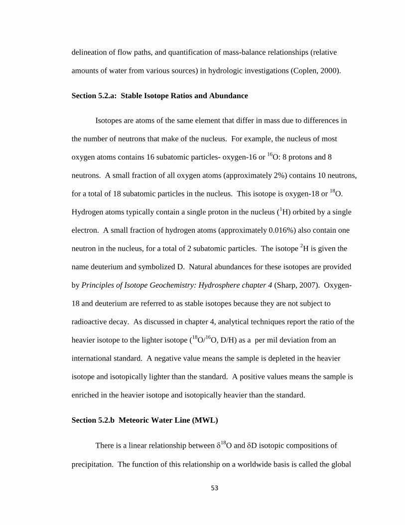
53

delineation of flow paths, and quantification of mass-balance relationships (relative

amounts of water from various sources) in hydrologic investigations (Coplen, 2000).

Section 5.2.a: Stable Isotope Ratios and Abundance

Isotopes are atoms of the same element that differ in mass due to differences in

the number of neutrons that make of the nucleus. For example, the nucleus of most

oxygen atoms contains 16 subatomic particles- oxygen-16 or 16

O: 8 protons and 8

neutrons. A small fraction of all oxygen atoms (approximately 2%) contains 10 neutrons,

for a total of 18 subatomic particles in the nucleus. This isotope is oxygen-18 or 18

O.

Hydrogen atoms typically contain a single proton in the nucleus (1H) orbited by a single

electron. A small fraction of hydrogen atoms (approximately 0.016%) also contain one

neutron in the nucleus, for a total of 2 subatomic particles. The isotope 2H is given the

name deuterium and symbolized D. Natural abundances for these isotopes are provided

by Principles of Isotope Geochemistry: Hydrosphere chapter 4 (Sharp, 2007). Oxygen-

18 and deuterium are referred to as stable isotopes because they are not subject to

radioactive decay. As discussed in chapter 4, analytical techniques report the ratio of the

heavier isotope to the lighter isotope (18

O/16

O, D/H) as a per mil deviation from an

international standard. A negative value means the sample is depleted in the heavier

isotope and isotopically lighter than the standard. A positive values means the sample is

enriched in the heavier isotope and isotopically heavier than the standard.

Section 5.2.b Meteoric Water Line (MWL)

There is a linear relationship between 18

O and D isotopic compositions of

precipitation. The function of this relationship on a worldwide basis is called the global

54

meteoric water line (GMWL). The GMWL can generally be defined by D= 8*18

O +

10 (Sharp, 2007). The GMWL was generated from thousands of analyses of precipitation

samples from the International Atomic Energy Agency network (Rozanski et al., 1993).

The intercept is known as the deuterium excess factor and can vary geographically. To

compensate for this a ‗local‘ meteoric water line (LMWL) is often defined for a given

study area. Because precipitation is the fundamental source for groundwater, the

interpretation of stable isotope data is often performed using a D versus 18

O plot with

the meteoric water line (MWL) as the reference (fig 5.1).

Figure 5.1 The relationship between D and 18

O of meteoric water,

as well as deviations from the MWL. From NMBGMR (Rawling,

2008).

55

A general feature of the GMWL is that precipitation in warmer climates will plot

toward the heavier end (less negative values), and precipitation from cooler climates plot

toward the lighter end (more negative values). Seasonal trends are also commonly

observed at a given location with winter precipitation at the lighter end and summer

precipitation toward the heavier end. However, this a simplified concept as there are

many interrelated factors controlling the isotope composition of precipitation.

A process that will cause water to deviate from the MWL is evaporation.

Evaporation is a nonequilibrium process that enriches the residual water such that the

D/18

O slope is less than 8, and often between 3 and 6 (fig 5.1). The slope of the

evaporation line (fig 5.1) is a function of humidity, temperature, salt concentrations and

other factors (Coplen, 2000).

Figure 5.1 also illustrates how the mixing of two water sources of distinct isotopic

compositions can be evaluated using the D/18

O plot. Two mixing waters will plot on a

straight line between the water sources end-members. The distance between the mixed

water and the end-members is proportionally related to the contribution from each end-

member.

Section 5.2.c: Factors Controlling the Isotopic Composition of Precipitation

The spatial and temporal variations of the isotope ratios in precipitation have their

origin in isotopic fractionation effects involved in evaporation from the ocean and the

environment influencing consequential condensation during transport through the

atmosphere. The variability is interpreted to be controlled by numerous inter-related

factors such as: surface air temperature, relative humidity in the atmosphere, amount of

56

precipitation, latitude, distance from the coast, seasonal variation and elevation of a given

area above sea level. These relationships have been observed by a worldwide survey of

isotopic composition of monthly precipitation by the International Atomic Energy

Agency in conjunction with the World Meteorologic Organizations, starting in the 1960‘s

(Rozanski, 1997). Each of these factors is in some way related to Rayleigh fractionation

during rainout of an air mass. Under Rayleigh conditions, liquid condenses in

equilibrium with the isotopic composition of the vapor, but then is removed from the

system (i.e. the cloud) as precipitation. The rainout process continually depletes the

remaining vapor fraction. Dansgaard (1964) empirically correlated the effect of these

factors to the average degree of rainout and the change in isotopic composition of

precipitation.

(1) Altitude Effect 18

O and D composition decrease with increasing altitude.

Higher altitudes are associated with cooler temperatures so air masses hold

less water (lower vapor fraction). Fractionation is also temperature dependant

and lower temperatures mean that Rayleigh fractionation is intensified.

(2) Latitude Effect 18

O and D composition decrease with increasing latitude

as rainout of air masses increases (lower vapor fraction) and temperature

decreases with latitude .

(3) Continental Effect 18

O and D composition decrease as air masses move

inland from the coast raining out over the continent (lower vapor fraction).

Another control on the continental effect is the ΔT decreases between the

source of the vapor and the precipitation location. During the winter this

effect increases.

57

(4) Amount Effect The greater the rainfall the more depleted 18

O and D

composition. Evaporation increases 18

O and D composition of light

precipitation compared to large rainfall events. Large rainout also means

lower vapor fraction remaining.

(5) Temperature This is so interrelated to the progression of rainout (lower

vapor fraction) during transport to higher latitudes (or altitudes) with lower

temperature that it is difficult to isolate its effects.

(6) Seasonal Variation Winter precipitation is typically depleted in 18

O and D

composition relative to summer rains in mid- and high latitudes. Seasonally

changing temperatures affect the extent of rainout (vapor fraction remaining).

Sources and travel paths of air masses can also change seasonally that affect

isotope compositions due to the continental effect.

The factors controlling isotopic compositions of precipitation are described in Principles

of Stable Isotope Geochemistry: Hydrosphere chapter 4 (Sharp, 2007) and

Environmental Tracers in Subsurface Hydrology: Isotope Engineering chapter 3

(Coplen, 2000).

Section 5.2.d: Identifying Sources of Recharge

Because the variability in the isotopic composition of precipitation is dependent

on recharge environment, 18

O and D can act as a fingerprint for sources of recharge to

the groundwater system. In a groundwater basin with sources of recharge at different

altitudes or with different seasonality for precipitation distinct end-members may be

58

identified. Different mechanisms of recharge will also affect the isotopic composition of

the groundwater. Higher rainfall events resulting in rapid infiltration through fast

transport pathways will have depleted isotopic signatures compared to slower infiltration

of lighter more scatter precipitation more affected by evaporation (Coplen, 2000).

Enrichment by evaporation of surface-water can be used as a trace for surface-water and

groundwater interactions (Coplen, 2000). Quantification of the contributing end-

members in a groundwater system can be determined based on mixing relationships.

Factors controlling the isotopic composition of precipitation such as changes in

temperature and precipitation patterns are also fundamental components to climate

change. This means isotopic shifts observed in groundwater can reflect changes in

recharge over time. The transition from the late Pleistocene to the present represents a

particularly significant shift in climate conditions for temperate-latitude regions. The

noble gases (Ne, Ar, Kr, and Xe) as well as oxygen and hydrogen isotopes have been

used as indicators for paleo-temperatures relative to present temperatures. Noble gas

ratios show evidence for recharge temperatures close to present values during most of the

Holocene. Alternatively, noble gas temperatures indicate for the last glacial maximum

(LGM) about 5.2 °C cooler temperatures compared to the Holocene (Stute et al., 1995).

This temperature shift was observed in a number of studies from Texas, New Mexico,

and Arizona. The difference in recharge temperature, as well as possibly other

interrelated factors: vegetation type, lower evaporation rates, higher humidity, or more

precipitation are shown to affect the oxygen and deuterium composition. In the San Juan

Basin, New Mexico, the isotopic composition of Pleistocene-age groundwater average

-3 per mil depletion in 18

O and -25 per mil depletion in D (Phillips et al., 1986). The

59

difference in 18

O and D, between the late Pleistocene to the Holocene groundwater

determined by Andrews and Lee (1979) is about -1.7 per mil in 18

O and D is depleted

by more than -8.4 per mil. These same waters all showed groundwater ages in excess of

10,000 yrs BP, and support evidence for recharge during a colder climate regime.

Section 5.3: Tritium as an Environmental Tracer

There are three isotopes of hydrogen. Hydrogen atoms typically contain a single

proton in the nucleus (1H) orbited by a single electron, also known as protium. A small

fraction of hydrogen atoms also contain one neutron in the nucleus, for a total of 2

subatomic particles, also known as deuterium. Tritium, the third naturally occurring

isotope of hydrogen, has one proton and two neutrons for a total of 3 subatomic particles

in the nucleus. The additional neutron in tritium imparts instability so that tritium is

subject to radioactive decay. Tritium (3H) decays by beta emission to

3He with a half-life

of 12.3 ± 0.02 years (Unterweger et al., 1980). Tritium can replace hydrogen in water to

form HTO (partially tritiated water) or T2O (tritiated water) (Solomon and Cook, 2000).

Because large amounts of tritium were blasted into the atmosphere during the

1950‘s-1960‘s atmospheric nuclear weapons testing, tritium can be used as an

environmental tracer to distinguish water recharged before, during or after the

atmospheric weapons testing period. Prior to 1950, the only source of tritium in

precipitation was from natural production in the upper atmosphere, largely through the

bombardment of nitrogen by the flux of neutrons in cosmic radiation. The natural (pre-

bomb) level of tritium in rainfall in Europe and North America was estimated by means

of measurements on vintage wines to be 3-6 tritium units (TU) in (Soloman and Cook,

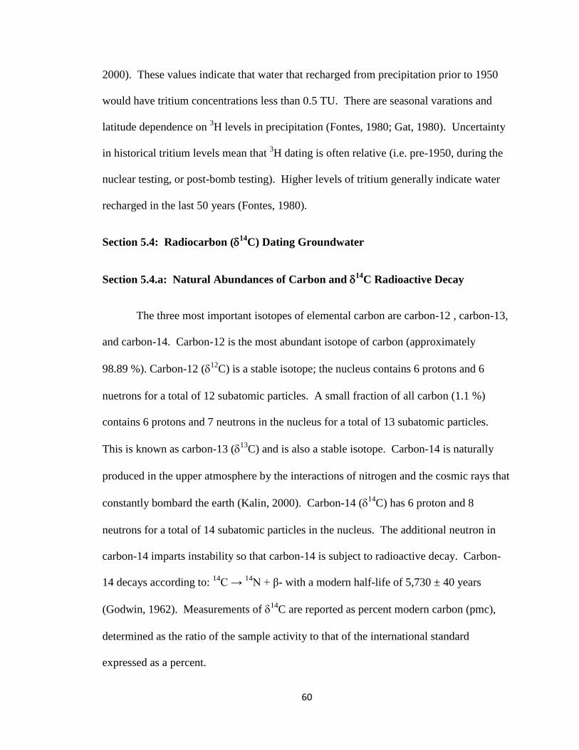
60

2000). These values indicate that water that recharged from precipitation prior to 1950

would have tritium concentrations less than 0.5 TU. There are seasonal varations and

latitude dependence on 3H levels in precipitation (Fontes, 1980; Gat, 1980). Uncertainty

in historical tritium levels mean that 3H dating is often relative (i.e. pre-1950, during the

nuclear testing, or post-bomb testing). Higher levels of tritium generally indicate water

recharged in the last 50 years (Fontes, 1980).

Section 5.4: Radiocarbon (14

C) Dating Groundwater

Section 5.4.a: Natural Abundances of Carbon and 14

C Radioactive Decay

The three most important isotopes of elemental carbon are carbon-12 , carbon-13,

and carbon-14. Carbon-12 is the most abundant isotope of carbon (approximately

98.89 %). Carbon-12 (12

C) is a stable isotope; the nucleus contains 6 protons and 6

nuetrons for a total of 12 subatomic particles. A small fraction of all carbon (1.1 %)

contains 6 protons and 7 neutrons in the nucleus for a total of 13 subatomic particles.

This is known as carbon-13 (13

C) and is also a stable isotope. Carbon-14 is naturally

produced in the upper atmosphere by the interactions of nitrogen and the cosmic rays that

constantly bombard the earth (Kalin, 2000). Carbon-14 (14

C) has 6 proton and 8

neutrons for a total of 14 subatomic particles in the nucleus. The additional neutron in

carbon-14 imparts instability so that carbon-14 is subject to radioactive decay. Carbon-

14 decays according to: 14

C → 14

N + β- with a modern half-life of 5,730 ± 40 years

(Godwin, 1962). Measurements of 14

C are reported as percent modern carbon (pmc),

determined as the ratio of the sample activity to that of the international standard

expressed as a percent.

61

Most laboratories report 14

C activity normalized for the isotope fractionation

effects of 13

C with a value of -25 per mil (Stuiver and Polach, 1977). This correction is

for more traditional use of radiocarbon dating (i.e. organic matter). In radiocarbon dating

groundwater most of the the effects on 13

C are from rock/water interactions where

dissolved inorganic carbon (DIC) is typically enriched compared to 13

C of -25 per mil.

This means radiocarbon dating of DIC in groundwater is better based on actual measured

14

C activity expressed in non-normalized (pmc). Normalized 14

C activities can be

converted to non-normalized values by the equation 5.1 (Mook and van der Plicht, 1999),

for measurements based on the 14

C/12

C ratio,

Equation 5.1

In this equation pmc is non-nomalized 14

C, pM is normalized 14

C, and 13

C is the

measured value. The 14

C pmc in table 5.1 has been de-normalized from the reported

values. This in the end is a minor correction only about 1 per mil difference.

Section 5.4.b: Concepts in Deriving Radiocarbon (14

C) Age of Groundwater

The radioactive carbon-14 is quickly oxidized to carbon dioxide (14

CO2). The

activity of 14

C in atmospheric CO2 gas is approximately 100 pmc (Fritz and Fontes,

1980). Atmospheric CO2 gas is incorporated into the groundwater system (as bicarbonate

62

H14

CO3-) during infiltration of recharge through the vadose zone (Kalin, 2000). As the

infiltration crosses the water table the dissolved inorganic carbon (DIC) is isolated from

the modern 14

C input from the atmosphere and soil zone reservoirs. As the water travels

along flow paths in the aquifer system the 14

C decays with time. This means the amount

of 14

C measured in the groundwater along a flow path, in association with its half life,

gives an age or the approximate time that has passed since the water recharged into the

aquifer system (equation 5.2). In relative terms, lower percent modern carbon (pmc)

indicates older groundwater. To quantitatively estimate groundwater age, radiocarbon

dating techniques interpret the distribution of a radiocarbon species in terms of a first-

order kinetic rate law of decay (Schwartz and Zhang, 2003). The groundwater age (t) is

determined by:

Equation 5.2:

Where is the half-life for decay, Ao is the activity assuming no decay, and Aobs is the

measured 14

C activity. The rate of decay (~ 5,730 yrs) means that radiocarbon dating

can be applied to groundwater from about 1,000 to 40,000 years old.

Section 5.4.c: Interpretation of Radiocarbon (14

C) Age of Groundwater

Carbon-14 (14

C) is not an ideal environmental tracer in that it is not necessarily

conservative in groundwater systems. Some reactive minerals (i.e., calcite) contain

inorganic carbon that can be transferred in and out of the groundwater. These

interactions act to reduce the 14

C activity in the water and need to be accounted for in

63

estimating the age (Shwartz and Zhang, 2003). Any age calculation (eqn. 5.2) is

meaningful only as long as Ao and Aobs only differ due to the effects of radioactive decay.

Ao (100 pmc) needs to be corrected for processes affecting 14

C activity in the

vadose zone during recharge. Typically two main factors are considered important in the

vadose zone. The infiltrating waters interaction with soil CO2 gas that typically has

higher pmc than atmospheric CO2 due to biologic activity (Brook et al., 1983). As well

as, the effects of dissolved CO2 reacting with carbonate minerals in the vadose zone of

the recharge area, resulting in increased dissolved inorganic carbon (Kalin, 2000). The

initial 14

C activity can be estimated using a number of isotope exchange and mass

balance approaches [see Kalin‘s chapter 4 on Radiocarbon Dating in, Environmental

Tracers in Subsurface Hydrology (2000)]. Alternatively, A0 can be assumed to be 85 ± 5

pmc based on numerous measurements of 14

C activity of groundwater recharge (Vogel

and Ehhalt, 1963; Vogel, 1967, 1970). And finally, Ao can be measured for any given

study area assuming confidence in a well delineated recharge area.

The 14

C activity measured along a flow path (Aobs) needs to be corrected for the

rock/water interactions that act as sources and sinks for carbon-14 as the water travels

through the aquifer system (Kalin, 2000). Well defined flow paths and geochemical

evolution are critical for accurate estimates of measured 14

C activity. Due to the many

geochemical interactions and hydrologic processes that can act as sources or sinks for 14

C

in a groundwater system, geochemical modeling is often applied in modern approaches to

radiocarbon dating. In particular, computer models such as NETPATH (Plummer et al.,

1994) can be used to quantify carbon mass transfer for determining the initial 14

C

activity and adjusting the observed 14

C activity.

64

Another important consideration in dating groundwater is that any water sample

collected contains a huge number of molecules. The path of each molecule containing

14C may be different due to dispersion/diffusion processes along the flow path. This

means that the measurement of 14

C activity in a water sample is actually a distribution

of all the 14

C activities from individual molecules. The reported values is the peak of

the distribution sometimes termed apparent groundwater age. The concept of an age

distribution has been widely applied in hydrology (Hooper, 2003; Loaiciga, 2004, and

McGuire and McDonnell, 2006).

Section 5.5: 34

SO4 as a Lithologic Tracer

There are four stable isotopes of sulfur (32

S, 33

S, 34

S, 36

S). The isotopes that are

commonly measured are 32

S and 34

S, because they are the most abundant at 95.03% and

4.19 %, respectively (Sharp, 2007). Often geologic units in an aquifer system contain

evaporitic gypsum. This means that the occurrence of groundwater can be traced using

the 34

S isotope content measured in sulfate from the groundwater as the isotopic

composition can be diagnostic of particular formations. Recharge enters the basin aquifer

system by infiltration of intermittent surface water flows and underflow along stream

channels as well as faults and fractures. Sulfate enrichment in the groundwater most

likely originate from dissolution of sulfate bearing minerals (gypsum/anhydrite) caused

by infiltrating meteoric waters into the extensive carbonate sequences. Dissolution of

evaporites does not involve significant sulfur isotope fractionation, thus 34

SO4 values of

the groundwater describe flow paths through isotopic signatures picked up from the

formation as the water moves through it (Krouse and Mayer, 2000).

65

Sample Location Goundwater Sample ID

D (per mil)

18

O (per mil)

Tritium 3H (TU)

13

C (per mil)

14

C (pmc)

34

SO4 (per mil)

Salt Basin Reserve -58.94 -9.38

Salt Basin Doll Day -60.87 -9.57 0.55 -10.30 51.74 10.26

Salt Basin Pinon Well -59.12 -9.34 1.27 -8.30 44.28

Salt Basin Webb House -71.85 -10.70 1.60 -9.80 67.70 11.70

Salt Basin Una -58.70 -9.43 1.14 -5.90 27.66 10.24

Salt Basin Runyan -68.44 -9.54 12.07

Salt Basin Cauhape -62.13 -9.94 0.27 -7.90 34.82 10.78

Salt Basin Jeffer's Well -59.96 -9.57 1.40 -7.80 29.04 11.28

Salt Basin Ellett Lower -62.87 -9.64 0.24 -5.70 14.37 9.98

Salt Basin Harvey Lewis Well 0.03 -4.50 19.74

Salt Basin Collins -65.94 -9.62 0.34 -5.20 19.62 11.68

Salt Basin New John A -63.19 -9.30

Salt Basin Evrage House -69.73 -9.55 0.01 -5.20 15.37 11.82

Salt Basin Hammock Well -68.11 -9.61 0.17 -2.70 22.92 11.43

Salt Basin Lewis -62.87 -10.23 0.18 -7.70 33.09 11.59

Salt Basin Butterfield Well -77.89 -12.15 0.11 -3.70 8.19 10.85

Salt Basin Bennett House -63.47 -10.26

Salt Basin Hunt 8 -69.97 -9.96 0.10 -5.20 22.52

Salt Basin Hunt C13 -65.53 -10.04 0.00 -6.00 22.50

Salt Basin Hunt C2 -63.64 -9.91 0.00 -5.40 26.09 11.35

Salt Basin Hunt House -69.01 -10.03 0.10 -5.30 22.78 11.85

Sacramento Mountains SM-0138 -60.00 -9.00 -8.90 85.76




Sacramento Mountains SM-1009 -60.00 -10.20 4.32 -12.90 92.65



Table 5.1 Evironmental tracers from groundwater in the Salt Basin and Sacramento Mountains

66

CHAPTER VI

GROUNDWATER SYSTEM CHARACTERIZATION

Section 6.1: Groundwater Chemistry

The groundwater chemistry dataset analyzed for this report is a compilation of

about 170 well samples which includes spring and well samples from the Sacramento

Mountains collected by New Mexico Bureau of Geology, and a general chemistry dataset

from wells throughout the Salt Basin compiled by Mayer for his 1995 dissertation. These

two sources supplement groundwater chemistry from about 25 well samples collected for

this study during a series of field trips through 2008--2009. See chapter 4 for a

discussion on the chemistry datasets and the distribution of sample sites (Fig 4.1). The

25 groundwater samples collected for this study define general flow paths along the

eastern side of the Salt Basin (Fig 6.1), starting in the recharge area of Sacramento

Mountains and extending south through the Piñon Creek watershed and Cornucopia

Draw, down to Crow Flats, and ending near both, the primary anthropogenic discharge

area of the Dell City Irrigation District, and the natural discharge area of the Salt Flats.

Because groundwater samples along these general flow paths on the eastern side of the

Salt Basin were sampled for stable isotopes and carbon-14 in addition to ion chemistry

this will be the principal flow path used for geochemical modeling to determine seepage

velocities and elucidate other important implications for recharge.

67

Figure 6.1 Distribution of sample points: Recharge (white) and Salt Basin(dark blue)

wells used for geochemical modeling through general sub-regions in the Salt Basin.

Digital Elevation Map (DEM) provided by the USGS National Elevation Dataset.

SM-0138

68

Section 6.1.a: Groundwater Temperature, Conductivity, and TDS

The temperature of groundwater in the Salt Basin ranges between 6 °C (in the

Sacramento Mountain wells and springs) and 25 °C (in the southern portion the Salt

Basin, near the Salt Flats). The average surface air temperature in the Sacramento

Mountains is 9 °C; however, mean annual air temperatures vary across the basin,

warming to 20 °C as elevation decreases to the south. The groundwater temperature

versus surface air temperature plot (fig 6.2) is atypical of shallow aquifers (it shows an

anomalously rapid increase of groundwater temperature with flow distance). This is

presumably because of the very deep vadose zone over the middle of the study area. The

groundwater temperature is roughly equivalent to the surface air temperature in the

recharge area where the aquifer is shallower. As the flow paths become deeper the

groundwater is heated due to thermal gradients (Reiter and Jordan, 1996). The increasing

trend in groundwater temperatures mirrors the increase in surface air temperature (fig

1.4) in its correlation to the topography of the basin (figures 6.3 and 6.4).

Groundwater temperatures near the range of mean annual surface air temperature

for the Sacramento Mountains (6-12 °C; fig 1.2) likely delineate recharge areas (fig 6.4).

Alternatively, anomalously high groundwater temperatures (i.e. Pinon and Ellett wells) in

the Salt Basin (fig 6.4) may indicate warmer deep groundwater upwelling (Reiter and

Jordan, 1996). Localized vertical groundwater flow may also affect the groundwater

chemistry at a well compared to the regional chemistry.

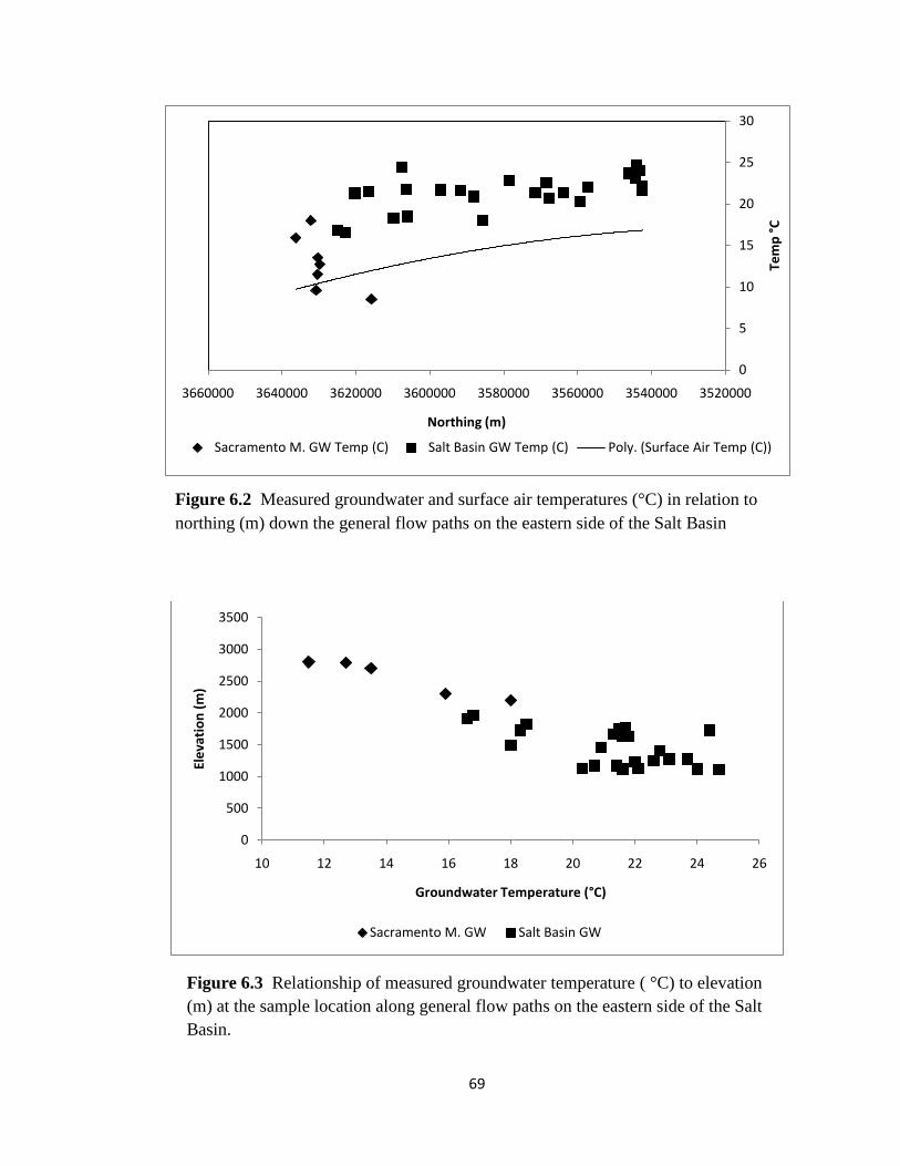
69

0

5

10

15

20

25

30

35200003540000356000035800003600000362000036400003660000

Tem

p °

C

Northing (m)

Sacramento M. GW Temp (C) Salt Basin GW Temp (C) Poly. (Surface Air Temp (C))

0

500

1000

1500

2000

2500

3000

3500

10 12 14 16 18 20 22 24 26

Ele

vati

on

(m

)

Groundwater Temperature (°C)

Sacramento M. GW Salt Basin GW

Figure 6.2 Measured groundwater and surface air temperatures (°C) in relation to

northing (m) down the general flow paths on the eastern side of the Salt Basin

Figure 6.3 Relationship of measured groundwater temperature ( °C) to elevation

(m) at the sample location along general flow paths on the eastern side of the Salt

Basin.

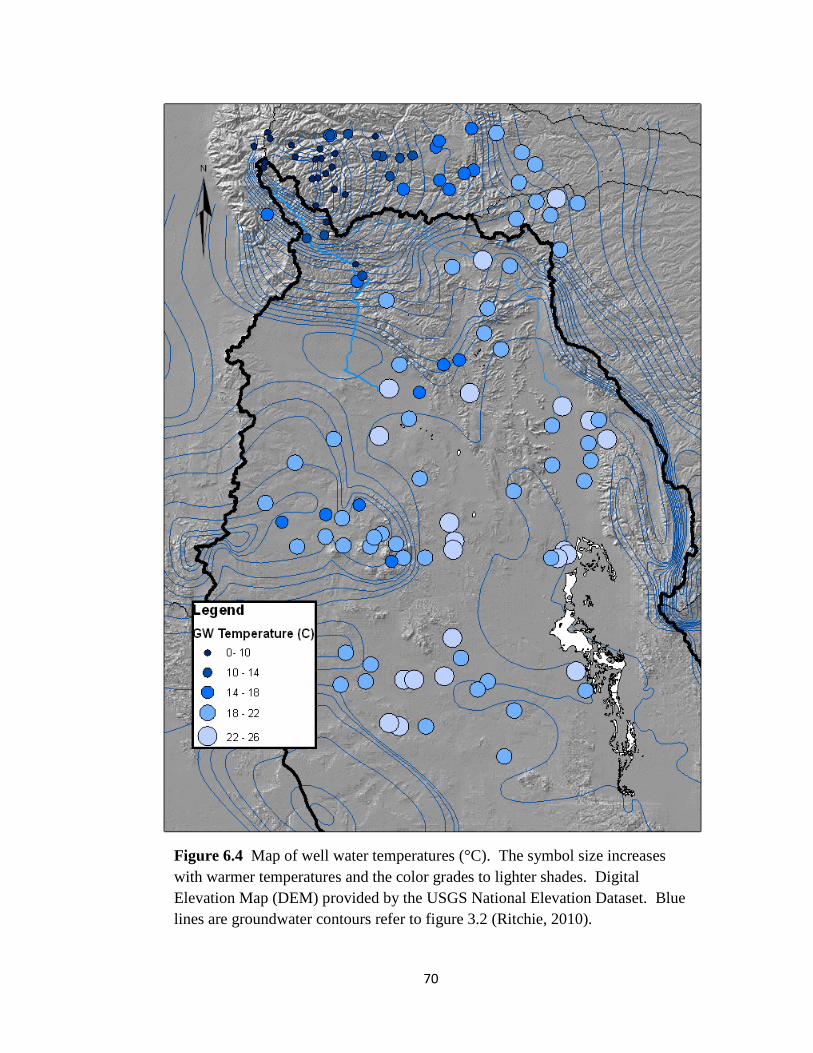
70

Figure 6.4 Map of well water temperatures (°C). The symbol size increases

with warmer temperatures and the color grades to lighter shades. Digital

Elevation Map (DEM) provided by the USGS National Elevation Dataset. Blue

lines are groundwater contours refer to figure 3.2 (Ritchie, 2010).

71

Total dissolved solids (TDS) is a relative measure of the total quantity of ions in

solution. Recharge areas will have low TDS (fig 6.5 and 6.6). TDS concentration will

increase with increased exposure for rock/water interactions and distance down the flow

path. The Otero Break (fig 2.3) corresponds to a zone of low TDS due to high

groundwater velocity funneling Sacramento Mountain recharge through the fracture zone

(Mayer, 1995).

0

500

1000

1500

2000

2500

35200003540000356000035800003600000362000036400003660000

Tota

l Dis

solv

ed

So

lids

(TD

S) m

g/L

Northing (m)

Sacramento Mountain GW Salt Basin GW

Pinon Well

Figure 6.5 Measured groundwater TDS (mg/L) in relation to northing (m)

down the general flow paths on the eastern side of the Salt Basin

72

Figure 6.6 Map of well water TDS concentration mg/L. The symbol size

increases with high concentration. Digital Elevation Map (DEM) provided by

the USGS National Elevation Dataset. Blue lines are groundwater contours refer

to figure 3.2 (Ritchie, 2010).

73

Section 6.1.b: Major Cations- Magnesium, Calcium, Sodium and Potassium

Increases in all the major cations are observed for the groundwater samples along

the flow paths on the eastern side of the Salt Basin (from the Sacramento Mountains

recharge area southeast to the discharge area of Dell City and the Salt Flats). Magnesium

concentrations (fig 6.7) steadily increase from about 10 mg/L to about 100 mg/L.

Calcium concentrations (fig 6.8) increase from about 90 mg/L to about 285 mg/L.

Sodium concentrations (fig 6.9) increase from about 5 mg/L to about 40 mg/L. A slight

overall increase in potassium concentrations (fig 6.10) is also observed from about 0.5

mg/L to about 2 mg/L.

0

20

40

60

80

100

120

140

160

35200003540000356000035800003600000362000036400003660000

Mag

ne

siu

m m

g/L

Northing (m)


Figure 6.7 Measured groundwater magnesium concentration (mg/L) in

relation to northing (m) down the general flow paths on the eastern side of

the Salt Basin

74

0

50

100

150

200

250

300

350

400

450

500

35200003540000356000035800003600000362000036400003660000

Cal

ciu

m (

mg/

L)

Northing (m)


0

10

20

30

40

50

60

70

80

90

100

35200003540000356000035800003600000362000036400003660000

Sod

ium

mg/

L

Northing (m)


Figure 6.8 Measured groundwater calcium concentration (mg/L) in relation

to northing (m) down the general flow paths on the eastern side of the Salt

Basin

Figure 6.9 Measured groundwater sodium concentration (mg/L) in relation


Basin

75

The distribution of the major cations from groundwater throughout the Salt Basin

is similar to the distribution of TDS content (fig 6.5). Magnesium (fig 6.11), sodium

(6.12), and calcium (6.13) concentrations are low through the Otero Break fault zone (fig

2.3). Consistent with the TDS the relatively freshwater appears to be an indication of

higher velocity flow paths preferentially channeling recharge from the Sacramento

Mountains to the Salt Basin graben (Mayer, 1995). Similar to groundwater

concentrations observed in the Sacramento Mountains concentrations through the Otero

Break are typically below: 50 mg/L for magnesium concentrations, 25 mg/L sodium

concentrations, and 120 mg/L for calcium concentrations.

The cation distribution for groundwater throughout the Salt Basin also mirrors the

TDS distribution in the prominent concentration increase in Otero Mesa and Diablo

0

0.5

1

1.5

2

2.5

3

3.5

4

4.5

35200003540000356000035800003600000362000036400003660000

Po

tass

ium

(m

g/L)

Northing (m)


Figure 6.10 Measured groundwater potassium concentration (mg/L) in


the Salt Basin

76

Plateau. In these regions concentrations are well above those seen on the eastern side of

the Salt Basin. Magnesium concentrations are between 100 and 200 mg/L. Sodium

concentrations have broad range between 50 and 500 mg/L. Similarly, calcium

concentrations are typically from 200 to 600 mg/L. Although higher concentration are

characteristic of the majority of groundwater samples in Otero Mesa, for all the major

cations there are some wells that have relatively low concentrations. This may be related

to some amount of recharge from the Cornudas Mountains, semi-perched aquifer

systems, or some kind of preferential flow feature. There is also freshwater associated

with the Diablo Plateau but this is likely related to eastward flow from the Hueco Bolson

(Kreitler, 1990).

77

Figure 6.11 Map magnesium concentration mg/L. The symbol size increases

with higher concentrations and the color grades to darker shades. Digital

Elevation Map (DEM) provided by the USGS National Elevation Dataset.

Blue lines are groundwater contours refer to figure 3.2 (Ritchie, 2010).

78

Figure 6.12 Map sodium concentration mg/L. The symbol size increases with

higher concentrations and the color grades to darker shades. Digital Elevation

Map (DEM) provided by the USGS National Elevation Dataset. Blue lines are

groundwater contours refer to figure 3.2 (Ritchie, 2010).

79

Figure 6.13 Map calcium concentration mg/L. The symbol size increases with




80

Section 6.1.c: Major Anions- Chloride, Sulfate, and Bicarbonate

Different trends for the major anions were observed for the groundwater samples

along the flow paths on the eastern side of the Salt Basin (from the Sacramento

Mountains recharge area southeast to the area of Dell City and the Salt Flats). Chloride

concentrations (fig 6.14) were relatively stable until rapid increasing near Dell City and

the Salt Flats. Sulfate concentrations (fig 6.15) steadily increased from about 20 mg/L to

600 mg/L. Bicarbonate concentrations (fig 6.16) slightly decreased from about 400 mg/L

to 200 mg/L.

The trends in the anion distribution throughout the Salt Basin were similar to

these trends. Chloride concentrations (fig 6.17) are relatively stable with much higher

concentrations near Dell City and the Salt Flats. The sulfate concentrations (fig 6.18) are

similar to the TDS distribution. There are low concentrations, similar to values observed

in the Sacramento Mountains, through the Otero Break. While Otero Mesa and Diablo

Plateau show much higher concentrations than those observed on the eastern side of the

Salt Basin. For Otero Mesa concentrations range from 900 mg/L to sometimes greater

than 2,000 mg/L. Bicarbonate concentrations (fig 6.19) are highest in the Sacramento

Mountains and Otero Mesa/Diablo Plateau and lowest near Dell City and the Salt Flats.

81

0

20

40

60

80

100

120

140

35200003540000356000035800003600000362000036400003660000

chlo

rid

e m

g/L

Northing (m)


0

200

400

600

800

1000

1200

35200003540000356000035800003600000362000036400003660000

Sulf

ate

mg/

L

Northing (m)


Figure 6.14 Measured groundwater chloride concentration (mg/L) in


the Salt Basin

Figure 6.15 Measured groundwater sulfate concentration (mg/L) in relation


Basin

82

0

50

100

150

200

250

300

350

400

450

35200003540000356000035800003600000362000036400003660000

Bic

arb

on

ate

mg/

L

Northing (m)


Figure 6.16 Measured groundwater bicarbonate concentration (mg/L) in


the Salt Basin

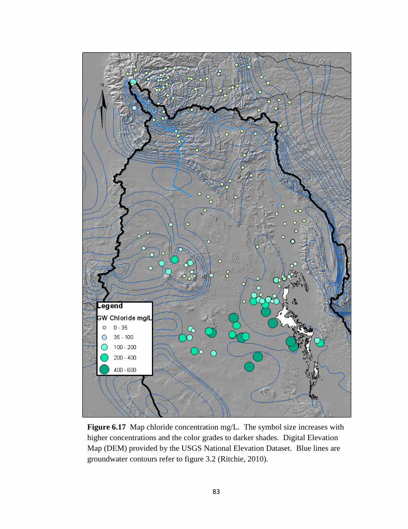
83

Figure 6.17 Map chloride concentration mg/L. The symbol size increases with




84

Figure 6.18 Map sulfate concentration mg/L. The symbol size increases


Elevation Map (DEM) provided by the USGS National Elevation Dataset.

Blue lines are groundwater contours refer to figure 3.2 (Ritchie, 2010).

85

Figure 6.19 Map bicarbonate concentration mg/L. The symbol size increases


Elevation Map (DEM) provided by the USGS National Elevation Dataset. Blue

lines are groundwater contours refer to figure 3.2 (Ritchie, 2010).

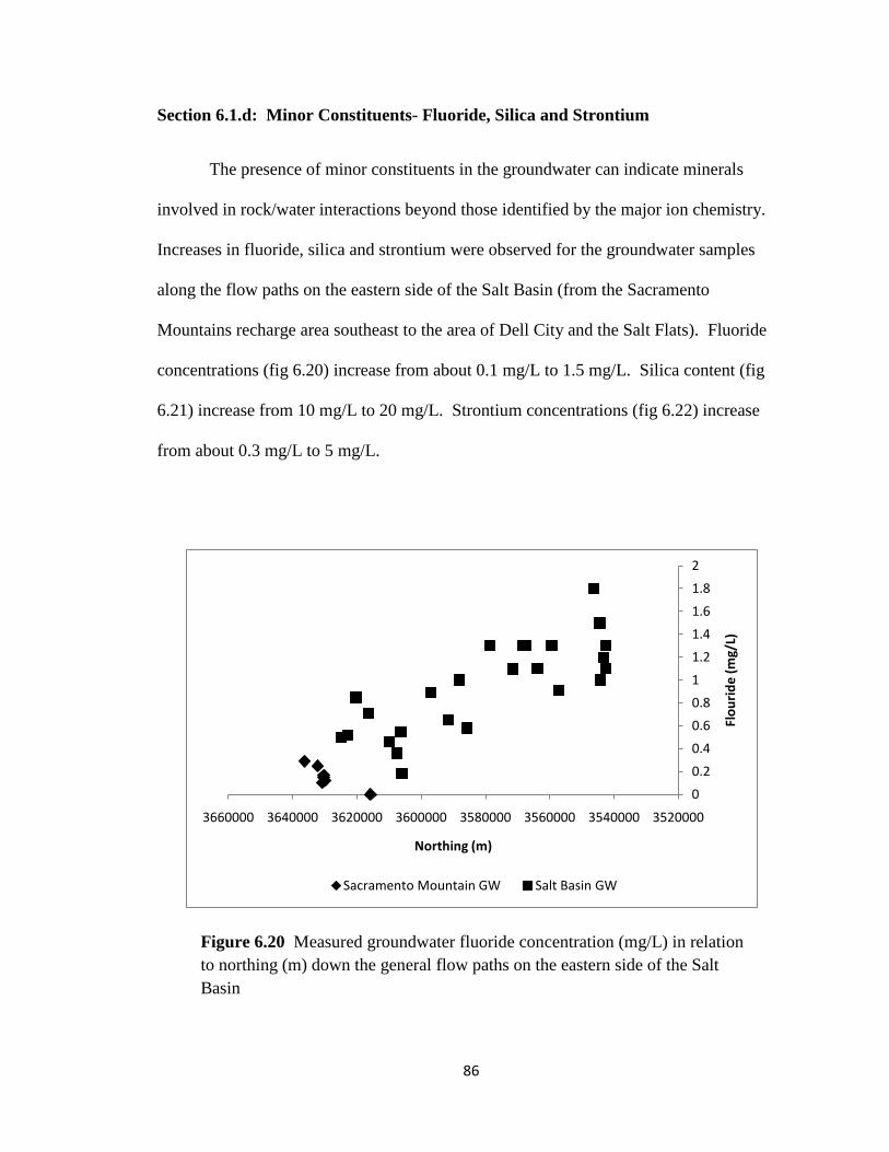
86

Section 6.1.d: Minor Constituents- Fluoride, Silica and Strontium

The presence of minor constituents in the groundwater can indicate minerals

involved in rock/water interactions beyond those identified by the major ion chemistry.

Increases in fluoride, silica and strontium were observed for the groundwater samples

along the flow paths on the eastern side of the Salt Basin (from the Sacramento

Mountains recharge area southeast to the area of Dell City and the Salt Flats). Fluoride

concentrations (fig 6.20) increase from about 0.1 mg/L to 1.5 mg/L. Silica content (fig

6.21) increase from 10 mg/L to 20 mg/L. Strontium concentrations (fig 6.22) increase

from about 0.3 mg/L to 5 mg/L.

0

0.2

0.4

0.6

0.8

1

1.2

1.4

1.6

1.8

2

35200003540000356000035800003600000362000036400003660000

Flo

uri

de

(m

g/L)

Northing (m)


Figure 6.20 Measured groundwater fluoride concentration (mg/L) in relation


Basin

87

0

5

10

15

20

25

35200003540000356000035800003600000362000036400003660000

Silic

a (S

iO2)

aq (

mg/

L)

Northing (m)


0

1

2

3

4

5

6

7

8

9

35200003540000356000035800003600000362000036400003660000

Stro

nti

um

(m

g/L)

Northing (m)


Figure 6.21 Measured groundwater silica SiO2aq concentration (mg/L) in


the Salt Basin

Figure 6.22 Measured groundwater fluoride concentration (mg/L) in relation


Basin

88

Section 6.2: Groundwater Chemistry Evolution

Section 6.2.a: Solute Sources and Sinks in the Aquifer System

As discussed in chapter 5.1, the chemical composition of groundwater is largely a

function of the lithology and mineralogy of the aquifer system. Ion chemistry trends are

diagnostic of the dominant reaction minerals along the flow paths. Along the flow paths

on the eastern side of the Salt Basin as the water evolves ion chemistry shows significant

increases in both magnesium and calcium concentration. The Salt Basin is

predominantly a carbonate aquifer system where calcite (CaCO3) and dolomite

[CaMg(CO3)2] are prominent components of the Permian San Andres and Yeso

formations. Dissolution of these minerals is a likely source for the increase in calcium

and magnesium observed down the flow paths.

(1) Calcite Dissolution:

CaCO3(calcite) + CO2(gas) + H20 Ca2+

+ 2HCO3-

(2) Dolomite Dissolution:

CaMg(CO3)2(dolomite) +2CO2(gas) + 2H2O Ca2+

+ Mg2+

+ 4HCO3-

Although, as Mayer (1995) points out in his discussion of the groundwater chemistry for

the Salt Basin, if only the dissolution of these two minerals were responsible for the ion

chemistry the molar ratio of (Ca2+

+Mg2+

)/(HCO3-) should be 1:2. This would also be the

ratio expected if weathering of calcium- and magnesium-bearing silicates such as

amphiboles pyroxenes were responsible for the increases. However, in the Salt Basin the

89

molar ratio of (Ca2+

+Mg2+

)/(HCO3-) plot above the 1:2 line indicating an additional

source of calcium or magnesium.

Although Figure 6.23 only illustrates the chemical evolution along the flow paths on

the eastern side of the Salt Basin, Mayer observed similar molar ratios in his analysis

(where water chemistry is largely from the Otero Mesa/Diablo Plateau, Crow Flats, and

Dell City region). Gypsum is a highly soluble mineral and present in both the San

Andres and Yeso formations (although more prevalent in the Yeso). This means the

additional source of calcium is likely a result of gypsum dissolution, as previously

suggested by Mayer (1995).

-5

-3

-1

1

3

5

7

9

0 2 4 6 8 10

Mg+

Ca

(mm

ol)

HCO3 (mmol)

Figure 6.23 Molar ratios of Ca2+

+Mg2+

vs HCO3- . 1:2 line would

correspond to the stoichiometric ratio for calcite and dolomite equilibrium

reactions.

1:2

90

(3) Gypsum Dissolution

CaSO4∙2H2O(gypsum) Ca2+

+ SO42-

Gypsum dissolution also accounts for the increase in sulfate observed down the flow path

(fig 6.15). To account for the additional Ca2+

from gypsum dissolution SO42-

is

subtracted from Mg2+

+ Ca2+

and plotted versus HCO3-. Based on reactions (1), (2) and

(3) this should yield a molar ratio of 1:2.

The dissolution and/or precipitation of calcite, and dissolution of dolomite and gypsum

are consistent with the groundwater chemistry along flow paths on the eastern side of Salt

Basin (from the Sacramento Mountains recharge area southeast to the area of Dell City

and the Salt Flats).

-5

-3

-1

1

3

5

7

9

0 2 4 6 8 10

Mg+

Ca

-SO

4 (m

mo

l)

HCO3 (mmol)

1:2

Figure 6.24 Molar ratios of Ca2+

+Mg2+

-SO42-

vs HCO3-. 1:2 line would

correspond to the stoichiometric ratio for calcite, dolomite and gypsum

equilibrium reactions.

91

In Mayer‘s (1995) analysis of the groundwater chemistry he shows that the

majority of the well chemistry he compiled plots below the 1:2 line for (Ca2+

+ Mg2+

-

SO42-

) versus HCO3-. Mayer (1995) discusses how this indicates an additional sink for

Ca2+

and/or Mg2+

, and suggests the possibility of cation exchange with Na+. To test his

hypothesis Mayer (1995) compares molar concentrations of Na+ - Cl

- versus (Ca

2+ + Mg

2+

- SO42-

- HCO3-/2). The quantity Na

+ - Cl

- is sodium derived from sources other than

halite dissolution, assuming all the chloride is derived from halite dissolution. The

quantity (Ca2+

+ Mg2+

- SO42-

-HCO3-/2) is the Ca

2+ and Mg

2+ from sources other than

carbonate and gypsum dissolution. Essentially he quantified the sodium and magnesium

plus calcium available for exchange. Mayer (1995) shows that for his chemistry dataset

this molar ratio defines a slope of -2 consistent with divalent cation exchange (i.e. Mg2+

or Ca2+

) with Na+ increasing at twice the rate. However, the majority of Mayer‘s dataset

was from groundwater from Otero Mesa and Diablo Plateau (fig 4.2). As discussed in

section 6.1 in these regions the groundwater chemistry observed is different than the

groundwater chemistry along the eastern side of the Salt Basin. Specifically, there are

much higher sodium concentrations in Otero Mesa/Diablo Plateau.

There is increasing in sodium concentration down the flow paths on the eastern

side of the Salt Basin (fig 6.9). A plot of the molar ratio of Na+ to Cl

- (fig 6.27),

assuming all chloride is the result of halite dissolution, would plot on a 1:1 line if only

halite dissolution were taking place down the flow path. There does appear to be a

source of sodium not associated with halite dissolution as the groundwater chemistry

molar ratios plot above the 1:1 line. However, a plot of Na+ - Cl

- versus (Ca

2+ + Mg

2+ -

92

SO42-

- HCO3-/2) shows no correlation for the groundwater chemistry, indicating that

cation exchange is not is not responsible for the additional sodium.

Alternative sources of the sodium could be from dissolution of detrital,

plagioclase feldspars (i.e. albite NaAlSi3O8) likely found within the clastic units of the

San Andres and Yeso formations. Typically, the pure potassium endmember orthoclase

(KAlSi3O8) forms in solid solution with albite (Chesterman, 1979) and may be

responsible for the increase in potassium (fig 6.10) down the flow path. Dissolution of

these feldspars would also explain the increase in silica content (fig 6.23) down the flow

path. The silica contents from groundwater on the eastern side of the Salt Basin are

0

0.5

1

1.5

2

2.5

3

3.5

4

4.5

5

0 1 2 3 4 5

Na

(mm

ol)

Cl (mmol)

Figure 6.25 Molar ratios of Na+ vs Cl

- . 1:1 line corresponds to the

stoichiometric ratio for halite dissolution.

1:1

93

typical (5-14 mg/L) for limestone and dolomites with trace clays and quartz present

(Langmuir, 1997).

Increases in minor constituents down the flow path on the eastern side of the Salt

Basin indicate the presence of other trace minerals. A trace mineral possibly present in

the aquifer system is fluorite (CaF2) due to the increase in fluoride concentration (fig

6.22) down the flow path. Fluorite may be associated with calcite and is a common

minor constituent in limestone (Chesterman, 1979). An increase in strontium

concentration (6.24) is also observed down the flow path. Celestite (SrSO4) is a likely

source of strontium. Celestite is mostly found in sedimentary rocks associated with

gypsum, anhydrite, and halite (Chesterman, 1979). Strontianite (SrCO3) could also be

present, which is a carbonate mineral with strontium (Langmuir, 1997).

Section 6.2.b: Evidence for Dedolomitization

The relative changes in ion chemistry of the groundwater provide information

about water-rock interactions that have taken place as the water travels along flow paths,

dissolving minerals in the rock. Classifying groundwater samples on a Piper diagram is

one way of identifying regions of chemically similar water and defining the evolution in

water chemistry along a flow system. Piper diagrams illustrate the distribution of relative

concentrations of cations (positively charged ions) and anions (negatively charged ions).

The relative abundance of cations with % meq/L of Mg2+

, Ca2+

and Na+

+ K+ are assumed

to be equal 100% and are plotted in the bottom left cation triangle. Similarly, the bottom

right anion triangle displays the relative abundance of Cl-, SO4

2-, and HCO3

-+CO3

2-.

94

Straight lines projected from the lower two triangles into the upper diamond define the

combined ion distribution.

The significant reaction minerals present in the Salt Basin carbonate aquifer

system are calcite (CaCO3), dolomite [CaMg(CO3)2], and anhydrite/gypsum (CaSO4).

This suggests the trends observed in the geochemical evolution illustrated by the Piper

diagram (fig 6.28) are diagnostic of dedolomitization taking place. In the Sacramento

Mountains the dominant groundwater type is calcium bicarbonate (Ca-HCO3), typical of

recharge through a carbonate aquifer system. As the water evolves south down the

principal flow path, the ion chemistry shows increases in both magnesium (Mg) and

sulfate (SO4), while bicarbonate (HCO3) slightly decreases. Back (1983) describes this

process as the dominant control on the chemical evolution of waters in a similar aquifer

system the Mississippian Pahasapa Limestone of the Madison aquifer (fig 6.29). His

paper shows evidence for how the dedolomitization process can take place across a

regional scale like the Salt Basin. Back (1983) summarizes the proposed mechanism for

dedolomitization from the explanations of a number of authors. As meteoric water

moves through an aquifer; calcite, dolomite, and anhydrite/gypsum go into dissolution at

different rates based on their geochemical stability. When the system becomes saturated

with calcite and dolomite, its evolution continues to be driven irreversibly by dissolution

of gypsum, which causes additional dissolution of dolomite and incongruent precipitation

of calcite. This causes increases in magnesium, and sulfate, while bicarbonate slightly

decreases. This evolution is consistent with the trends observed in the Salt Basin. With

the exception of Ellett well that also showed anomalous temperature (fig 6.4).

95

Figure 6.26 Piper diagram of Salt Basin well chemistry. The sampled well

waters plot on a linear trend indicating increasing magnesium and sulfate

concentrations. The trend is indicative of dedolomitization as described in Back

(1983). The star is an outlier to the trend (Ellett well)

96

Section 6.2.c: Water Chemistry of the Otero Mesa

The water chemistry in Otero Mesa reflects significant increases in sulfate, as

well as, sodium concentrations. This is evident from the position of the Otero Mesa

water chemistry samples on the Piper diagram (fig 6.28) as well as in the maps of sodium

(fig 6.12) and sulfate (fig 6.18) concentrations throughout the Salt Basin. The

gypsiferous Yeso formation dominates in this region which likely explains the higher

sulfate concentrations. In general this region is associated with more evaporitic deposits,

Figure 6.27 Piper diagram groundwater chemistry of Pahasapa

Limestone of the Madison Aquifer. The trend is indicative of

dedolomitization as described in Back (1983).

97

which also explains higher concentrations of chloride compared to other areas in the Salt

Basin that are equidistant from the Salt Flats. The introduction of sodium to the

groundwater system here may indicate dissolution of carbonate or gypsum minerals

accompanying calcium or magnesium exchange with sodium; which was previously

discussed (6.2.a). Alternatively, these waters are also in close proximity to the Cornudas

Mountains which may mean the introduction of sodium is a result to syenite weathering

processes.

Section 6.2.d: Brine Evolution Effects

The existence of the Salt Flats is a function of the Salt Basin being a closed un-

drained basin. In this type of system, precipitation falling on the mountain front enters

the groundwater through fractured rocks, talus slopes, or alluvial fan deposits. Valleys in

the basin and range province are tectonic troughs that often lack a subsurface outlet; the

water returns to the surface through playas, where it is discharged to the atmosphere by

evapotranspiration. Runoff in this system will drain internally, with no outlet except the

atmosphere (Duffy 1988). The locally depressed playas or salt flats tend to lie in chains

on the east or west edges of the basin; probably originating as shallow or intermittent

lakes that filled slight depressions in the valley floor. They often lie along fault trends.

The level of the Salt Flats is generally lower than the surrounding ground level, with

elevations around 1100 meters, which is about at the water table in the lower Salt Basin.

Closed and undrained basins can be considered self-contained hydrologic systems, with

water and energy exchange primarily with the atmosphere. These dynamics can result in

forced convective flow that leads to a hydrodynamic connection between the

groundwater and the atmosphere at the Salt Flats.

98

As the groundwater in the Salt Basin moves closer to the discharge area at the Salt

Flats the effects of brine evolution are evident. When pore fluids are removed by

evaporation from the Salt Flats the concentration of dissolved solids increases, such that

certain minerals are removed from solution by precipitation and the remaining solution

becomes enriched or depleted in one ion or another. The Eugster-Hardy model (1978)

does a good job of explaining the Salt Basin brine evolution. Calcite, the least soluble

mineral is the first to precipitate removing bicarbonate and carbonate from the water.

Gypsum precipitates next, where initial molar ratios dictate sulfate build-up and calcium

depletion. Ultimately, relatively dilute inflow waters evolve to water types dominated by

chloride and sulfate for the anions, balanced by sodium and magnesium for the cations.

This progression can be observed in the Piper diagram trends moving from the Dell City

area to the Salt Flat groundwater samples (fig 6.28). The effects of brine evolution are

also apparent in the map of chloride concentrations throughout the Salt Basin (fig 6.17).

The Salt Flats produce evaporite deposits of gypsum and halite, as well as carbonate

minerals such as calcite, dolomite, and magnesite (Boyd 1982). In the Dell City area

groundwater is likely influenced by back flushing of salts from irrigation TDS

concentrations reach 6500 mg/L (Mayer, 1995). At the Salt Flats where groundwater is

discharging through evapotranspiration TDS concentration can be in excess of 250,000

mg/L (Boyd, 1982).

Section 6.3: Geochemical Reactions and Mass Transfer

The rock/water interactions that will dominate in the subsurface as the

groundwater flows through the aquifer are controlled by the departure from chemical

equilibrium conditions of the water with respect to the minerals present, as discussed in

99

chapter 5. Saturation indices for groundwater down the principal flow path analyzed for

the Salt Basin were calculated using the USGS geochemical modeling program

NETPATH. Interpretation of the values of saturation index for the important minerals in

the system--calcite, dolomite, and gypsum--shows that the significant reactions are

consistent with dedolomitization being the dominant control on the water chemistry

(Back and Hanshaw, 1971). The saturation index for gypsum/anhydrite (fig 6.30) shows

that water is significantly undersaturated in the Sacramento Mountain recharge area;

while the saturation index increases progressively with increased distance along the flow

path. The saturation indices indicate irreversible dissolution of gypsum/anhydrite; in as

much as equilibrium conditions are never reached. The saturation index for dolomite (fig

6.31) indicates that the water in the recharge area is undersaturated, but, that with

increasing dissolution of gypsum, the water reaches equilibrium or slightly above

equilibrium. The water is close to, or above, equilibrium for calcite (fig 6.32).

If there was no gypsum/anhydrite present in the Salt Basin aquifer system, calcite

and dolomite would dissolve to equilibrium. Given only these two phases, at low

temperatures, calcite is more unstable than dolomite and would likely attain equilibrium

faster. Under these conditions it would be expected that some of the calcite originally

dissolved would precipitate when dolomite saturation is approached. However, because

gypsum is dissolving the water reaches supersaturation with respect to calcite and

dolomite, due to the calcium ions put into solution by the dissolution of gypsum (CaSO4).

This constant addition of calcium from the gypsum forces precipitation of calcite

(CaCO3) due to the common-ion effect (Back, 1983). When calcite precipitates it causes

100

-3

-2.5

-2

-1.5

-1

-0.5

0

35200003540000356000035800003600000362000036400003660000

Gyp

sum

SI

Northing (m)


-2

-1.5

-1

-0.5

0

0.5

1

1.5

2

35200003540000356000035800003600000362000036400003660000

Do

lom

ite

SI

Northing (m)


Figure 6.28 Saturation index [log(IAP/KT)] for gypsum equilibria as a function

of distance down flow path for Salt Basin well samples. Shaded blue indicates

equilibrium.

Figure 6.29 Saturation index [log(IAP/KT)] of dolomite equilibria as a function


equilibrium.

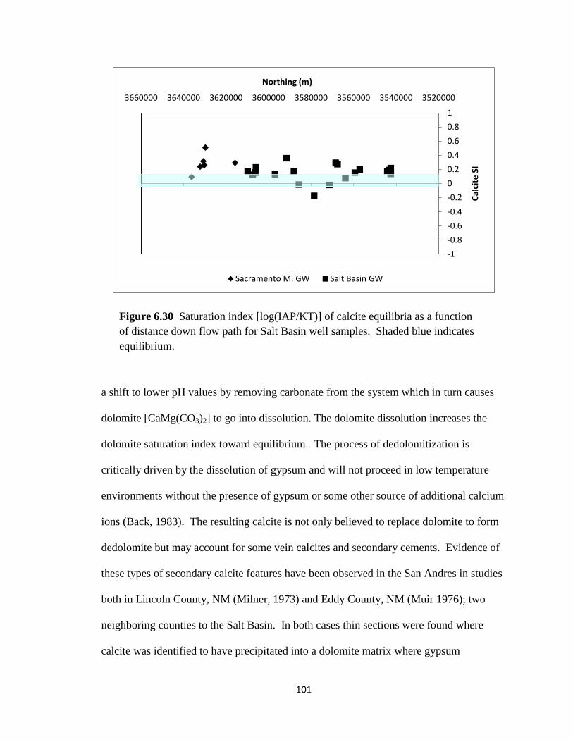
101

a shift to lower pH values by removing carbonate from the system which in turn causes

dolomite [CaMg(CO3)2] to go into dissolution. The dolomite dissolution increases the

dolomite saturation index toward equilibrium. The process of dedolomitization is

critically driven by the dissolution of gypsum and will not proceed in low temperature

environments without the presence of gypsum or some other source of additional calcium

ions (Back, 1983). The resulting calcite is not only believed to replace dolomite to form

dedolomite but may account for some vein calcites and secondary cements. Evidence of

these types of secondary calcite features have been observed in the San Andres in studies

both in Lincoln County, NM (Milner, 1973) and Eddy County, NM (Muir 1976); two

neighboring counties to the Salt Basin. In both cases thin sections were found where

calcite was identified to have precipitated into a dolomite matrix where gypsum

-1

-0.8

-0.6

-0.4

-0.2

0

0.2

0.4

0.6

0.8

1

35200003540000356000035800003600000362000036400003660000

Cal

cite

SI

Northing (m)


Figure 6.30 Saturation index [log(IAP/KT)] of calcite equilibria as a function


equilibrium.

102

dissolution took place (fig 6.33). Although, it should be noted that overall the

dedolomitization reaction results in net dissolution which may enhance permeability in

the aquifer system.

Figure 6.31 Evidence for secondary calcite replacing gypsum in a dolomite

matrix found in the San Andres unit near the Salt Basin. In example a.) the

gypsum matrix is black and the white marked M is the secondary calcite. In

example b.) the gypsum matrix is red and the small white mineralization marked D

is the secondary calcite.

a.)

b.)

103

The dedolomitization reaction process is as follows:

(a) 2H2O + 2CO2(gas) → 2H2CO3→ 2H+ + 2HCO3

-

(b) 2H+ + 2HCO3

-+ CaSO4(gypsum) + CaMg(CO3)2(dolomite) → 2Ca

2+ + SO4

2- + Mg

2+ + 4HCO3

-

(c) 2Ca2+

+ SO42-

+ Mg2+

+ 4HCO3- → SO4

2- + Mg

2+ + 2CaCO3(calcite) + 2H

+ + 2HCO3

-

In the Madison aquifer this process was observed to coincide with an increase in PCO2 as

well as a decrease in pH (Plummer, 1991). However, in the Salt Basin system the PCO2

(fig 6.34) and pH (fig 6.35) are relatively stable down the flow path.

-3

-2.5

-2

-1.5

-1

-0.5

0

35200003540000356000035800003600000362000036400003660000

PC

O2

Northing (m)


Figure 6.32 Variation in log partial pressure of carbon dioxide as a function of

distance down flow path measured from wells in the Salt Basin.

104

Another defining characteristic of the dedolomitization reaction process is the

Mg/Ca ratio. Dolomite is near equilibrium at 25 °C in low temperature groundwater that

is also in equilibrium with calcite and has Mg/Ca ratio equal to one (Hanshaw, 1971).

When Mg/Ca ratios are greater than one, dolomite precipitates, and for ratios less than

one dolomite goes into dissolution. The significance of this relationship is that it is the

mechanism by which gypsum drives the dedolomitization. The dissolution of gypsum

introduces the calcium to the system that keeps the Mg/Ca ratio lower than one. The

groundwater in the Salt Basin remains consistently below a Ma/Ca ratio of one, as seen in

figure 5.17. This coupled with the precipitation of calcite forces dolomite dissolution. If

either gypsum dissolution stopped or calcite precipitation stopped the water would attain

equilibrium with dolomite and dedolomitization would cease. Equilibrium conditions for

6

6.2

6.4

6.6

6.8

7

7.2

7.4

7.6

7.8

8

35200003540000356000035800003600000362000036400003660000

pH

Northing (m)


Figure 6.33 Variation in pH as a function of distance down flow path measured

from wells in the Salt Basin.

105

this system are best represented as a range (figures 6.30-6.32) because the temperature

dependence of the saturation conditions of dolomite and calcite are not necessarily well

constrained, especially in dynamic equilibrium conditions with each other.

Section 6.4: Chemical and Mineralogical Comparison using SaltNorm

SNORM is free USGS software that will calculate a salt norm from the chemical

composition of natural water. The salt norm is the quantitative ideal equilibrium

assemblage of minerals that would crystallize if the water were evaporated 100% at 25 °C

and 1 bar pressure under atmosphere partial pressure of CO2. It quantitatively distributes

the program‘s 18 acceptable solutes into normative salts that are assigned from 63

0

0.1

0.2

0.3

0.4

0.5

0.6

0.7

0.8

0.9

1

3530000 3540000 3550000 3560000 3570000 3580000 3590000 3600000 3610000 3620000

Mg/

Ca

mm

ol

Northing (m)

Figure 6.34 Mg/Ca molar ratio along the groundwater flow path. The Mg/Cl

ratio is a significant control for the dedolomitization process.

106

possible normative salts to allow only stable associations based on the Gibbs Phase Rule,

available free energy values, and observed low temperature associations (Bodine, 1986).

SNORM characterization of groundwater samples from the Salt Basin will be

used in a comparison between the geochemical evolutions of waters analyzed for the

Madison aquifer, as a test for the importance of dedolomitization as a water chemistry

control. Different areas within the Salt Basin have distinct water chemistry

characteristics that are associated with the groundwater. The water chemistry

characteristics of each region are a function of both its evolutionary point along a flow

path and rock/water interactions controlled by the lithology. Each unique area might

even be considered a hydro-chemical facies. Like a geologic facies it is a distinct unit

which forms under certain conditions of sedimentation which reflect a particular process

or environment. To illustrate these hydrologic facies spatially within the two basins,

water chemistry data was analyzed using Salt Norm. The normative salt compositions

were averaged for each region giving distinct distributions based on mineral percent.

In the Salt Basin the normative salt distribution (fig 6.37) for the Sacramento

Mountains and Piñon area is largely calcite (CaCO3) , dolomite [CaMg(CO3)2] , and

gypsum/anhydrite (CaSO4). This composition is controlled primarily by CO2-carbonate

mineral reactions with some gypsum/anhydrite dissolution as precipitation recharges

through the San Andres and/or Yeso formations. As the groundwater flows south

through Cornucopia Draw the normative distribution of dolomite increases, while calcite

disappears. The appearance of magnesite (MgCO3), like the increase in dolomite, is a

reflection of the increase in magnesium as the water evolves. The Crow Flats have water

107

chemistry consistent with relatively mature waters in which dissolution of

gypsum/anhydrite dominates over dissolution of the carbonate minerals. Dolomite is no

longer present in the normative salt distribution, leaving magnesite as the only carbonate-

Figure 6.35 Salt Norm % mineral compositions and their spatial distribution

in the Salt Basin. It is a quantitative mineralogic comparison of natural waters.

Progression of the mineral compositions down the flow path is consistent with

Ca>Mg:HCO3 to Ca>Mg:SO4>HCO3 to Na>Ca>Mg:Cl>SO4>HCO3 which

describes the dedolomitization reaction path.

108

containing mineral. The percentage of gypsum/anhydrite significantly increases, and the

mineral epsomite (MgSO4) appears for the first time in the distribution. For these waters,

salts with sulfate present in the mineral compositions make up at least 80% of the total

distribution.

The major minerals in the Madison Limestone are calcite, dolomite, and

gypsum/anhydrite, like the Salt Basin. The equilibrium speciation calculations for the

saturation indices of these minerals (Plummer, 1991) are comparable to those of the Salt

Basin. In Plummer‘s 1991 report of the hydrology of the Madison Limestone he

discusses these thermodynamic controls on the trends in the water chemistry that result

from the dedolomitization reaction as discussed by Back and others (1983). The full

dedolomitization reaction path is described as progressing from predominantly

Ca>Mg:HCO3 to Ca>Mg:SO4>HCO3 to Na>Ca>Mg:Cl>SO4>HCO3 waters. This

evolution is consistent with that of the Salt Basin which is clearly illustrated by

comparing the chemical evolution between the two aquifers by the Piper diagrams. The

dedolomitization reaction process is also observed in the progression of the mineral

compositions calculated using Salt Norm down the Salt Basin flow path as well as that of

the Madison Aquifer. Each mineral distribution in the Salt Basin marks a distinct point in

the chemical evolution that corresponds to a matching point in the chemical evolution in

the Madison Limestone.

109

Section 6.5: Salt Basin Solute Controls by Faults and Structural Features

The Salt Basin is a block-faulted graben, where the central part of the basin is at

lower elevation than the surrounding mesas, plateaus, and mountains. The Sacramento

Mountains are generally considered the dominant source of recharge for the Salt Basin

(Mayer, 1995; Huff, 2006; Sharp, 1995). This means that like many semiarid basins, the

most significant contribution to recharge to the basin aquifer is flux across the mountain-

front block (Wilson, 2004). Generally, the Sacramento Mountain fault block marks the

northern boundary of the Salt Basin groundwater system. Mayer (1995) has discussed

how a 300 foot scarp at the boundary of the Otero Mesa and the Tularosa Valley forms a

Figure 6.36 Salt Norm % mineral compositions and their spatial distribution in

the Madison Aquifer. Dedolomitization is the dominant control on the

geochemical evolution in the Madison Aquifer.

110

major surface-water divide and the western margin of the groundwater flow system. He

interpreted the eastern boundary of the basin fixed at the graben of the Salt Basin which

is juxtaposition between the low-permeability basin fill and highly, fractured carbonates.

In Mayer‘s PhD dissertation (1995) he presents data in support of faulting and fracturing

within the structure of the Salt Basin playing a significant role in the control of

groundwater movement. In between the Otero Mesa and the Salt Basin graben lies a

prominent faulted and fractured south-west facing scarp, known as the Otero Break

(Goetz, 1985; Black, 1975). This feature is characterized by a series of west-dipping

normal faults that are an extension of the Sacramento Mountains. Otero Break gradually

disappears to the southeast. This feature is the result of two stages of deformation: first

right-lateral shear and extension during the Paleozoic along northwest-oriented fault

zones and second west- oriented extension, beginning during the Neogene (Goetz, 1985).

Within the flow system, the groundwater flows preferentially to the southeast, parallel to

the high-permeability fracture zone (Mayer, 1995). Groundwater chemistry throughout

the basin has been used to identify a broad zone of relatively fresh water (based on TDS)

extending from the Sacramento Mountains southeast down to the Salt Flats near Dell

City, TX (Mayer, 1995). This trend is present along the Otero Break fracture, which

Mayer attributes to large-scale channeling of Sacramento Mountain recharge along

faulted and fractured conduits.

Based on the water chemistry evolution defined by the dedolomitization reaction

process, there are specific ions present in the groundwater that can be used as a proxy for

residence time in the groundwater system. The increase in aqueous magnesium and

sulfate in the groundwater is a time-dependent process related to the dissolution of

111

dolomite and gypsum as the water travels through the aquifer system. Contour plots of

the concentrations of these two ions (figures 6.39 and 6.40) illustrate how the

groundwater chemistry in the Salt Basin varies systematically in space. These trends

identify other structural controls on the movement of the groundwater in the Salt Basin

system in addition to the major channeling along the Otero Break.

Structural features that appear to control the movement of groundwater are

generally characterized as either a barrier to flow or zones of enhanced permeability. The

prominent features that correlate with solute movement in the Salt Basin are the

Stevenson fault in the north, the Otero fault and Diablo Plateau in the west, and the Dog

Canyon fault zone to the east (fig 2.3). The Otero Break controls the groundwater flow in

the center of the basin. Considering that the Stevenon fault is the possible westward

extension of the Guadalupe fault zone, it is consistent with the water chemistry that this

fault acts as a barrier to flow from the north into the Salt Basin; just as the Guadalupe

fault zone marks an eastern boundary for the groundwater system. The Stevenson fault is

characterized by high-angle, down-to-the-south normal faulting, as previously cited. This

may be responsible for low permeability behavior or act as a short circuit to the flow

system as aquifer units may be displaced. At the southern extent of the Guadalupe fault

zone, along the Algerita Escarpment of the Guadalupe Mountains is the Dog Canyon

fault zone. This corresponds to a region of what appears to be relatively freshwater input

to the Salt Basin from the Guadalupe Mountains. It is difficult to say whether this

corresponds to groundwater influx from the regional flow system of the Guadalupe

Mountains or as surface water infiltration through the Dog Canyon drainage network.

112

During the Permian, down-to-the-northeast faulting occurred along several

northwest trends, one of which is the Otero fault. This feature corresponds to a broad

zone of high concentration of the chemical tracers with relatively freshwater channeling

along either side. There are two likely scenarios to explain the solute distribution

resulting from that of the Otero fault zone. One is enhanced permeability along the

western and eastern margins of the fault zone channeling water around what would have

to be a relatively low permeability zone in the center caused by the inherent trends in the

nature of the displacement (Caine, 1996). Alternatively, Nutt (1997) discusses how this

region corresponds to the western edge of the buried Pedernal uplift. This is associated

with significant thinning of the Yeso aquifer unit above the buried uplift, where water

may preferentially channel around this feature. Solute distributions also show an influx

of relatively fresh water moving northeast to the Salt Flats in Texas across the aquifer

system of the Diablo Plateau. This is consistent with Krietler and others (1990). This

water encounters the Babb flexure where increased permeability could be related to

Leonardian reefs that ring the fault deformation, as previously cited.

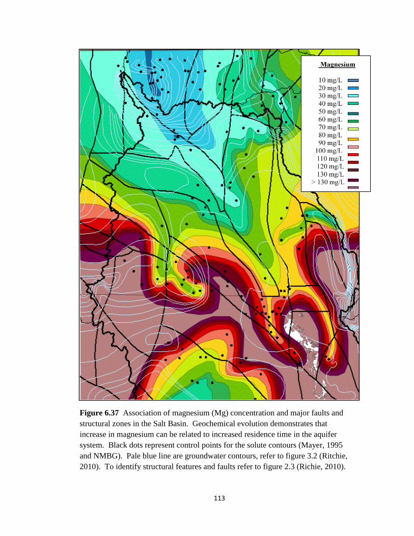
113

Figure 6.37 Association of magnesium (Mg) concentration and major faults and

structural zones in the Salt Basin. Geochemical evolution demonstrates that

increase in magnesium can be related to increased residence time in the aquifer

system. Black dots represent control points for the solute contours (Mayer, 1995

and NMBG). Pale blue line are groundwater contours, refer to figure 3.2 (Ritchie,

2010). To identify structural features and faults refer to figure 2.3 (Richie, 2010).

114

Figure 6.38 Association of sulfate (SO4) concentration and major faults and

structural zones in the Salt Basin. Geochemical evolution demonstrates that

increase in sulfate can be related to increased residence time in the aquifer system.

Black dots represent control points for the solute contours (Mayer, 1995 and

NMBG). Pale blue line are groundwater contours, refer to figure 3.2 (Ritchie,

2010). To identify structural features and faults refer to figure 2.3 (Richie, 2010).

115

CHAPTER VII

STABLE ISOTOPES AND THEIR IMPLICATIONS FOR RECHARGE

Section 7.1: Recharge Environment

Stable isotope ratios of oxygen (18

O) and hydrogen (D) are useful

environmental tracers that can act as a fingerprint for sources of recharge to a

groundwater system. As discussed in chapter 5.2, the isotopic composition of

precipitation depends on certain conditions of the recharge environment: surface air

temperature, relative humidity in the atmosphere, amount of precipitation, latitude,

distance from the coast, and elevation of a given area above sea level (5.2.c). For the Salt

Basin, this means that precipitation will have different isotopic signatures depending on

whether it falls during the summer or winter, and where it takes place in the basin. The

mechanism for recharge will also affect the isotopic signature of the groundwater (5.2.d).

Understanding these relationships can distinguish between recharge from the Sacramento

Mountains, the Guadalupe Mountains, and lowlands in the Salt Basin based on their

recharge environment.

The Sacramento Mountains rise to elevations of 2,500 to 2,900 m with average

precipitation of about 27 cm/yr. Based on a recent study of the hydrogeology of the

Sacramento Mountains by the New Mexico Bureau of Geology, the recharge

environment is described as follows (Rawling, 2009). The Sacramento Mountains

receive the majority of their rainfall during the monsoon season from May to October.

116

This rainfall pattern is a result of orographic effects and the higher temperatures

associated with these seasons. The precipitation is generated from the forced vertical

movement of moist air up the orographic slope caused by the daytime heating of the

mountain surface. The air parcels cool and expand as they are lifted, resulting in

condensation and potentially precipitation. Winter storms are frontal storms that

originate in the eastern Pacific and lose most of their moisture as they travel across the

mountains of California and Arizona. Recharge in average precipitation years is largely

from snow melt that has infiltrated into the stream/spring system and subsequently

undergone evaporation in stream channels and spring-fed wetlands before infiltrating into

the groundwater system. There is an additional source of recharge from extreme storm

events during some monsoon seasons that contributes to the aquifer system through short,

transient flow paths, such as fractures systems, that are not significantly affected by

evaporation. The recharge from the Sacramento Mountains enters the Salt Basin aquifer,

primarily, as a subsurface flux across the mountain-front-block.

The Guadalupe Mountains are lower in elevation than the Sacramento Mountains.

The Guadalupe Mountains border the east side of the Salt Basin with elevations of about

1,400 to 2,600 m with average precipitation of about 19 cm/yr. The mechanisms for

recharge from the Sacramento Mountains into the Salt Basin are different than those of

the Guadalupe Mountains. Most studies of the groundwater system in the Guadalupe

Mountains have concluded that the regional flow is to the east. The mountain front faults

adjacent to the Salt Basin graben are generally considered to be barriers to subsurface

flow. This means the precipitation entering the Salt Basin from the Guadalupe

Mountains will be diffuse near-surface flow that is transmitted along the steep slope via

117

ephemeral drainage networks such as arroyos; or as subsurface interflow from small

catchments along the mountain front.

The elevation of the Salt Basin graben is about 1,100 m with average precipitation

of about 10 cm/yr. The little moisture the lowlands do receive is primarily during

summer monsoon showers. However, it is likely most of this precipitation is lost to

evaporation as spring and summer are characterized by extremely high temperatures,

often above 37 °C (100 °F), and severe dust storms. If there was recharge, a significantly

evaporated signal would be expected in the groundwater; with the exception of fast-

transport infiltration during flood events.

Section 7.2: Distribution of D and 18

O in the Salt Basin Groundwater System

Because precipitation is the fundamental source for groundwater, the

interpretation of stable isotope data is often performed using a D versus 18

O plot with

the Meteoric Water Line (MWL) as the reference line; This is discussed in chapter 5.3.b.

For this study of the Salt Basin it is more informative to use a Local Meteoric Water Line

(LMWL), where the slope and y-intercept may vary slightly from the GMWL due to

local climatic conditions. In the Sacramento Mountains the LMWL (fig 7.1) is defined

by D = 8.38*18

O + 22.77, based on local precipitation collected regularly since 2006

by the New Mexico Bureau of Geology (Rawling, 2009). The New Mexico Bureau of

Geology estimated an evaporation line (5.2.c) for the Sacramento Mountains as

D = 5.47*18

O + 12.03 (fig 7.1), based on surface-water compositions measured from

streams and wetlands in the area (Rawling, 2009).

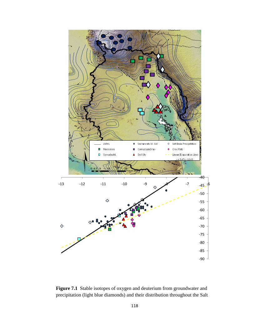
118

-90

-85

-80

-75

-70

-65

-60

-55

-50

-45

-40

-13 -12 -11 -10 -9 -8 -7 -6

Figure 7.1 Stable isotopes of oxygen and deuterium from groundwater and

precipitation (light blue diamonds) and their distribution throughout the Salt

Basin.

119

Typically, winter precipitation is depleted in D and 18

O relative to summer

rains (5.2.c). This trend is observed in the isotopic composition of precipitation collected

in the Sacramento Mountains (Rawling, 2009). However, for many groundwater systems

the meteoric D- 18

O signature transferred during recharge tends to be an average over

the summer and winter isotopic signatures. As rainwater infiltrates into the unsaturated

zone, movement and mixing through convoluted paths leads to a smoothing out of the

seasonal variations. This is thought to particularly apply to karstic and fractured

limestones environments like the Salt Basin. In these types of systems it has been

observed that infiltrating water, traversing a 10-15 m thick unsaturated zone retains less

than 5% of seasonal variation (Yonge, 1985). This is consistent with groundwater

measured for the Sacramento Mountains which generally plots between the seasonal

extremes. Most of the Sacramento Mountains groundwater also plots between the

LMWL and the evaporation line (fig 7.1, blue circles). This suggests that the mixing

process during infiltration also tends to smooth out differences in the signature between

waters infiltrating through streams and springs that have an evaporative signature, and

fast transport infiltration waters that have not undergone evaporation (Rawling, 2008).

For this study precipitation was collected from four points within the Salt Basin

including the Pinon area, the rim of the Guadalupe Mountains, Cornucopia Draw, and

near Dell City (fig 7.1, light blue diamonds). The precipitation collected in August is

consistent with the isotopic composition of summer precipitation for the Sacramento

Mountains and plots between -65 and -55 per mil for D and -9 and -10 per mil 18

O.

The precipitation collected in October show highly variable compositions and all plot left

of the LMWL.

120

Groundwater samples collected along the general flow paths on the eastern side of

the Salt Basin system were also analyzed for stable isotope composition. Those in the

Piñon area (fig 7.1, green squares), extending down through Cornucopia Draw (fig 7.1,

purple squares), plot along with groundwater samples from the Sacramento Mountains.

That is between the LMWL and the evaporation line, indicating a mixing process

between evaporated and non-evaporated recharge. There are two exceptions in these

regions that appear depleted with respect to the others; one from the Piñon area (Webb H.

well), and one from Cornucopia Draw (Runyan). The well depth of the Cornucopia Draw

sample is quite deep; as it was originally drilled as an oil well. The deeper well may

penetrate a deeper long flow path, or maybe a different geologic facies which might

explain the discrepancy. There is no well depth information for the Piñon area sample,

which makes it more difficult to interpret.

The majority of groundwater samples collected from Crow Flats down to the Dell

City area appear isotopically depleted compared to the other waters of the Salt Basin.

These waters plot below the evaporation trend for the Sacramento Mountains. If the

slope of the evaporation trend has remained constant through time, the original

composition of the precipitation (i.e. the intercept with the LMWL) would be

significantly depleted compared to that of modern groundwater in the Sacramento

Mountains. Two possible scenarios explain the observed depletion in these, as well as

the exceptions in the more northern Salt Basin groundwater samples. One is that

mountain-front recharge from the Guadalupe Mountains might have entered the southern

extent of the basin during extreme winter precipitation events, where surface runoff is

transmitted along arroyos and alluvial fans into the Salt Basin at the Crow Flats. In the

121

case of the northern exceptions, winter floods might have entered through drainage

networks extending from the southern Sacramento Mountains. The other explanation is

that residence times in the Salt Basin are long, and that some groundwater in the basin

may have recharged under a very different climatic environment.

Two other anomalous stable isotope compositions come from the groundwater

samples collected in the more western part of the basin, in the vicinity of the Cornudas

Mountains. These samples plot directly on the LMWL; but one is significantly depleted

compared to the other. This is interesting particularly because of how close (less than a

mile) the two wells were to each other. This might seem like an indication that modern

recharge is present because of their positions relative to the LMWL and the variability

between them. However, this does not seem consistent with the percent modern carbon

measured for these wells which was below 14 pmc (table 5.1), generally indicating these

are very old waters (5.4). They also lie within the very high concentration regions for

magnesium and sulfate which also indicates long older more evolved water (figure 6.39

and 6.40).

Section 7.3: Implications for Recharge from the Guadalupe Mountains

Surface runoff from the Guadalupe Mountains during extreme storm events could

contribute significant amounts of isotopically light water which would explain the

depletion in Crow Flats and Dell City isotope compositions. The factors that would

cause this depletion would be related to what is different about this source of recharge

compared to that of the Sacramento Mountains. Most importantly, in the case of

Guadalupe Mountain recharge, only extreme storm events are being considered

122

significant sources; in which case the infiltration would be depleted primarily due to the

―amount effect‖ (5.2.c). Additionally, if the storm event was from winter precipitation it

would originate over the Pacific Ocean as opposed to monsoon storms which come from

the Gulf Coast. This would further deplete the isotopic signature due to the ―continental

effect‖ (5.2.c). More intense rainfall events will also be associated with faster infiltration

with less evaporation effects also resulting in more depleted the isotopic signature (5.2.b).

The introduction of water with this type of signature along the Guadalupe

Mountains bordering Crow Flats could explain the depletion observed in the lower Salt

Basin groundwater. Fresh water introduced from the Guadalupe Mountains along the

Dog Canyon Fault zone is also consistent with solute distributions for magnesium and

sulfate that were used as proxies for residence time. A similar type of recharge might

also explain the depletion in the Piñon area well. However, this scenario is less

consistent with the depletion observed in the deep (~1000 m) well in Cornucopia Draw.

Section 7.4: Implications for Paleo-Recharge

There are a couple of aspects of the groundwater chemistry in the Crow Flats and

Dell City region that are not completely consistent with the hypothesis of Guadalupe

Mountain recharge during extreme storm events as a significant source to the

groundwater. One apparent contradiction to new water recharging into this area is the

low tritium levels observed in the groundwater (fig 7.2). Tritium as an environmental

tracer is discussed in chapter 5.3. The tritium levels in the Sacramento Mountains range

from 2.97 to 10.4 TU (Rawling, 2009). These are consistent with of post-bomb recharge,

indicating the groundwater is typically less than 50 years old. The relationship between

123

tritium concentrations and carbon-14 pmc (fig 7.3) is also consistent with the higher

tritium concentrations in the Sacramento Mountains being modernly recharged water

whereas the low tritium concentrations have pmc associated with older water. Carbon-14

and groundwater ages are discussed in chapter 5.4.

Figure 7.2 Tritum (TU) distribution throughout the Salt Basin. Light

green are from the Sacramento Mountains, blue are from the Salt Basin.

124

In the Salt Basin, tritium levels fall below 0.5 TU over a relatively short distance

as the groundwater flows into the lowlands of the basin, below the Piñon area. At Crow

Flats there does not appear to be an influx of modern water, based on the low tritium

concentrations. The carbon-14 is also low (<25 pmc) (table 5.1) for the groundwaters of

Crow Flats and Dell City. Percent modern carbon versus D values (fig 7.4) shows a

positive correlation between decreasing pmc and depletion in the deuterium values. This

evidence is not completely consistent with modern recharge entering the Salt Basin

lowlands through runoff from the Guadalupe Mountains. However, the discontinuity in

age interpreted using tritium which is limited to less than 50 years old, and carbon-14

which measures on the order of thousands of years old, could mask the presence of

recharge from the Guadalupe Mountains due to mixing processes.

0

10

20

30

40

50

60

70

80

90

100

0 1 2 3 4 5 6

14 C

(P

MC

)

3H (TU)

Figure 7.3 Tritium concentrations in the Salt Basin groundwater as a function of 14

C pmc

125

The alternative explanation for the depletion in the stable isotope values observed

in the lower extent of the Salt Basin would be that discrete water parcels along a flow line

may reflect changes in recharge environment over time. As previously discussed (5.2.d),

recharge temperatures during the last glacial maximum (LGM) were about 5-6 °C cooler

in New Mexico and Texas (Stute et al., 1995). The cooler recharge environment has been

shown to correspond to a shift in isotopic composition of Pleistocene aged groundwater

to more depleted values. In the San Juan Basin, New Mexico, the isotopic composition

of the Pleistocene-age groundwater averages -3 per mil depletion in 18

O and -25 per mil

depletion in D (Phillips et al., 1986). The extent of the depletion in the Salt Basin

groundwater isotope compositions can be analyzed with two basic approaches.

Figure 7.4 Groundwater carbon-14 pmc as a function of deuterium isotope ratios

(per mil)

126

The first is that the slope of the evaporation line is used to project onto the

LMWL the reconstructed composition of each Salt Basin sample before evaporation took

place (fig 7.5). If groundwater from the lower Salt Basin is paleo-recharge and if the

slope of the evaporation trend has remained constant through time, the original

composition of the precipitation (i.e. the intercept with the LMWL) would illustrate the

depletion of paleo-precipitation compared to modern precipitation in the Sacramento

Mountains. The blue field (fig 7.5) is the weighted annual average of the isotopic

composition of precipitation from the Sacramento Mountains measured from 2006 to

2008 (NMBGMR; Rawling, 2008). There are large seasonal variations in the isotopic

-100

-95

-90

-85

-80

-75

-70

-65

-60

-55

-50

-15 -14 -13 -12 -11 -10 -9 -8

D

(p

er

mil

)

18O (per mil)

Pinon Cornucopia Draw Crow Flats Dell City Cornudas

Figure 7.5 Oxygen and deuterium isotope ratio projected with the slope of the

evaporation line to determine intercept with the LMWL. Hollow symbols are measured

and solid symbols are projected isotopic composition. Blue field is annually weighted

isotopic composition of precipitation from the Sacramento Mountains measured 2006-

2008 (NMBGMR; Rawling, 2008)

127

composition of precipitation measured in the Sacramento Mountains. The annual

weighted average isotopic composition is the average of the isotopic values of all samples

collected at a single location over one year, weight by the sample volumes. The hollow

symbols (fig 7.5) are the measured groundwater isotopic compositions from the Salt

Basin and the solid symbols are the projected intercept with LMWL using the

evaporation line. Based on the projected compositions, the depletion in precipitation for

Crow Flats and Dell City groundwater samples compared to modern precipitation in the

Sacramento Mountains range from about -5 to -25 per mil in D and -1 to -4 per mil in

18

O.

An alternative approach is to compare the 18

O and D values from the

Sacramento Mountains and the Salt Basin with both modern precipitation and paleo-

recharge from the Franklin and Organ Mountains, west of the Salt Basin. In the Hueco

Bolson Aquifer (Fig 1.1) groundwater recharged from the Franklin and Organ Mountains

show two distinct groupings of 18

O and D composition (Eastoe, 2007). The group

associated with modern recharge show stable isotope compositions around -9 and -65 per

mil 18

O and D, respectively. The second group is depleted by about -1 per mil and -10

per mil, for 18

O and D, respectively. The carbon-14 data from this study show that the

groundwater with the lower stable isotope compositions are most likely late Pleistocene

precipitation (Eastoe, 2007). The comparison of shifts in both 18

O and D values from

modern recharge to paleo-recharge in the Franklin and Organ mountains is pretty

comparable to the shift observed in the Salt Basin from the Sacramento Mountains

modern precipitation to the groundwater of Crow Flats and Dell City (fig 7.6).

128

The groundwater from the Hueco Bolson Aquifer that correspond to the isotopic

composition of modern precipitation from the Franklin and Organ Mountains are labeled

―Franklin M. GW modern‖, ―Fort Bliss GW modern‖, and ―Chaparral GW modern‖.

For each of these locations average groundwater values are plotted where whisker bars

are the ±1σ (standard deviation). The groundwater from the Hueco Bolson Aquifer that

correspond to the isotopic composition of paleo-recharge are labeled ―Franklin M. GW

paleo‖, ―Fort Bliss GW paleo‖ and ―Chaparral GW paleo‖. Again for each of these

locations average groundwater values are plotted where whisker bars are the ±1σ

(standard deviation). The average isotopic composition of modern Sacramento Mountain

precipitation is labeled ―S.M. precipitation‖ with whisker bars of the ±1σ (standard

Figure 7.6 Depletions in 18

O and D compositions from modern Sacramento

Mountain precipitation to groundwater in the Salt Basin compared to the

depletions observed between modern precipitation and pale-groundwater in the

Franklin and Organ Mountains. Whisker bars are the ±1σ (standard deviation)

when averages were used.

129

deviation). The average isotopic composition of modern recharge from groundwater in

the Sacramento Mountains is labeled ―Sacramento M. GW modern‖ with whisker bars of

the ±1σ (standard deviation). The rest of the points are individual measurements from

groundwater within the Salt Basin. The groundwater from the southern Salt Basin, such

as Crow Flats and Dell City, appear to trend toward the paleo-groundwater compositions

observed in the Organ and Franklin Mountains (fig 7.6).

The overall depletion down the flow paths on the eastern side of the Salt Basin

(starting in the Sacramento Mountains and moving southeast to Dell City and the Salt

Flats) is about -1 per mil in 18

O (fig 7.7) and -10 per mil in D (fig 7.8). These shifts are

about the same as those between modern recharge and paleo-recharge in the Franklin and

Organ Mountains.

-13

-12

-11

-10

-9

-8

-7

35200003540000356000035800003600000362000036400003660000

1

8 O (

pe

r m

il)

Northing (m)


Figure 7.7 Measured groundwater 18

O content (per mil) in relation to

northing (m) down the general flow paths on the eastern side of the Salt

Basin

130

The stable isotope evidence for the presence of paleo-groundwater in the Salt

Basin seems consistent. This hypothesis could also explain the depletion observed in the

deep well in Cornucopia Draw. It is possible this well intercepts a deeper, longer,

regional flow path along which paleo-groundwater may still be present in the more

northern extent of the basin. This hypothesis does not explain the depletion in the Piñon

area well, as it has high percent modern carbon, and tritium levels above 1.5 TU. This

depletion is more likely evidence for modern recharge in the Sacramento Mountains

during extreme storm events where runoff is propagated to at least the foothills in this

region before it infiltrates along fast transport-fracture pathways.

-87

-77

-67

-57

-47

-37

-27

-17

-7

35200003540000356000035800003600000362000036400003660000

D

(p

er

mil)

Northing (m)


Figure 7.8 Measured groundwater D content (per mil) in relation to

northing (m) down the general flow paths on the eastern side of the Salt

Basin

131

Section 7.5: Principal Component Analysis/End Member Mixing Analysis

This section discusses mixing relationships of stable isotopes determined in order

to identify what sources contribute significantly to the Salt Basin groundwater.

However, it should be noted, the Salt Basin aquifer is not a well mixed system. Flow in

the Salt Basin is dominantly by means of large and small scale fracture systems, leading

to limited mixing along the flow paths. As will be discussed further in chapter 8.5.b., this

means flow in the Salt Basin more closely follows a piston-flow model compared to a

mixed-reservoir model. For the purposes of the end member mixing analysis, mixing

refers to: the introduction of new water along flow paths (i.e. Guadalupe Mountain or

storm event recharge), the presence of water along piston-flow paths where isotopic

compositions reflect change in recharge condition over time, or density driven mixing

near the Salt Flats.

Understanding quantitatively how much contribution there is of paleo-

groundwater, or even Guadalupe Mountain recharge, to the Salt Basin presents a difficult

problem. It has been shown that the mixing of two water sources of different isotopic

compositions can be evaluated by looking at a plot of D and 18

O. A water sample that

is a mixture of two isotopically distinct waters will have an isotopic composition that

plots on a straight line that connects the two end member water sources (5.2.b). For

example, how groundwater in the Sacramento Mountains plots between the LMWL and

the evaporation line suggesting it is a mixture of evaporated and un-evaporated sources of

recharge. The proportion of mixing can be quantified based on where the point lies on

the mixing line between the two end members. In the Salt Basin there are more than two

end members to consider as contributing sources to the groundwater system. Each

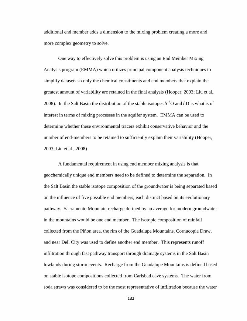
132

additional end member adds a dimension to the mixing problem creating a more and

more complex geometry to solve.

One way to effectively solve this problem is using an End Member Mixing

Analysis program (EMMA) which utilizes principal component analysis techniques to

simplify datasets so only the chemical constituents and end members that explain the

greatest amount of variability are retained in the final analysis (Hooper, 2003; Liu et al.,

2008). In the Salt Basin the distribution of the stable isotopes 18

O and D is what is of

interest in terms of mixing processes in the aquifer system. EMMA can be used to

determine whether these environmental tracers exhibit conservative behavior and the

number of end-members to be retained to sufficiently explain their variability (Hooper,

2003; Liu et al., 2008).

A fundamental requirement in using end member mixing analysis is that

geochemically unique end members need to be defined to determine the separation. In

the Salt Basin the stable isotope composition of the groundwater is being separated based

on the influence of five possible end members; each distinct based on its evolutionary

pathway. Sacramento Mountain recharge defined by an average for modern groundwater

in the mountains would be one end member. The isotopic composition of rainfall

collected from the Piñon area, the rim of the Guadalupe Mountains, Cornucopia Draw,

and near Dell City was used to define another end member. This represents runoff

infiltration through fast pathway transport through drainage systems in the Salt Basin

lowlands during storm events. Recharge from the Guadalupe Mountains is defined based

on stable isotope compositions collected from Carlsbad cave systems. The water from

soda straws was considered to be the most representative of infiltration because the water

133

could be collected as soon as it entered the cave, minimizing evaporation and exchange

with the cave environment (Ingraham, 1990). The contribution of a paleo-groundwater

end member is defined by the average stable isotope compositions of groundwater found

in the Franklin and Organ Mountains interpreted to have paleo-origins (Eastoe, 2007).

The final end member is that of the Salt Flats. This composition is distinct in its highly

evaporated signature and was averaged from pore water collected at 30, 60, 120, 122 cm

depth within the playa (Chapman, 1984).

For the Salt Basin a 2-dimensional mixing subspace represents a good model ―fit‖

using 18

O and D as conservative tracers in the system. This means three end members

are required to explain most of the variability in the system. The majority of the Salt

Basin groundwater samples fall within a mixing space defined by Sacramento Mountain

recharge, rainfall infiltration through lower elevation drainage networks, and paleo-

groundwater, figure 7.9. Outliers to this mixing space include groundwater from the

Crow Flats which fall into a mixing space defined by Sacramento Mountain recharge,

paleo-groundwater, and Guadalupe Mountain recharge, figure 7.10. As well as, the Dell

City area groundwater, which is defined by Sacramento Mountain recharge, paleo-

groundwater, and the Salt Flats, figure 7.11.

Webb house and Runyan wells are two outliers that can‘t be defined by any

combination of the end member mixing. As previously noted, Runyan is a very deep

well which appears to intercept a unique flow path compared to other waters in the

system. While Webb house maybe a reflection of a recent localized storm event that

affected the well water just prior to collection and can‘t be matched to more regional

compositional trends.

134

Figure 7.9 Mixing between Sacramento M. groundwater, Salt Basin precipitation,

and Paleo-groundwater end-members. These end-members explain the majority of

the variability in 18

O and D from the Salt Basin well samples.

Figure 7.10 Mixing between Sacramento M. groundwater, Paleo-groundwater, and

Guadalupe M groundwater end-members. These end-members explain the variability

in 18

O and D from the Salt Basin well samples in the Crow Flats.

135

The percent contribution of each end member in the above mixing spaces is

illustrated in figure 7.12. These should not be taken too literally as the end-members are

defined more theoretically, especially the paleo-groundwater and the Guadalupe

Mountain groundwater. However, in general it looks like wells in the northern extent of

the basin are mostly defined by Sacramento Mountain recharge and fast track

precipitation events. While the Dell City and Crow Flat waters are more consistent with

paleo-groundwater signatures, with only slight influence by the Guadalupe Mountains

and the Salt Flats.

Figure 7.11 Mixing between Sacramento M. groundwater, Paleo-groundwater, and

Salt Flat end-members. These end-members explain the variability in 18

O and D

from the Salt Basin well samples near Dell City.

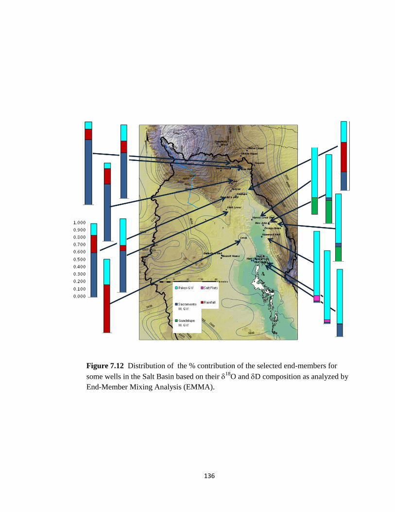
136

Figure 7.12 Distribution of the % contribution of the selected end-members for

some wells in the Salt Basin based on their 18

O and D composition as analyzed by

End-Member Mixing Analysis (EMMA).

137

CHAPTER VIII

GEOCHEMICAL MODELING TO ESTIMATE RECHARGE USING CARBON-14

Section 8.1: Radiocarbon Dating in Groundwater Systems

Although certain hydrodynamic and geochemical processes can cause difficulties

in the interpretation of groundwater age, many hydrogeologic setting have been

investigated where radiocarbon dating has successfully elucidated information on flow

velocity and recharge rates based on groundwater ages in an aquifer system (see chapter

5.4 for a discussion on radiocarbon dating systematics). Ideally multiple environmental

tracers are used to characterize the residence time of groundwater in an aquifer system

where corroboration between a set of tracers overcomes the uncertainties associated with

each tracer as an individual.

Due to the many geochemical interactions and hydrologic processes that can act

as sources or sinks for 14

C in a groundwater system, geochemical modeling is often

applied in modern approaches to radiocarbon dating. The geochemical modeling

techniques employed for the Salt Basin aim to reduce uncertainties in two critical

components of 14

C dating: determination of the initial 14

C activity of infiltration as it

crosses the water table (Ao), and the extent of rock/water interactions occurring along

flow paths and their effect on the 14

C activity.

138

Section 8.2: Definition of Recharge Chemistry

In the Salt Basin, flow paths used for geochemical modeling begin in the

Sacramento Mountains and extend south, to the east of the Otero Break, through Piñon

Creek watershed and Cornucopia Draw, through Crow Flats, ending near Dell City and

the Salt Flats (fig 6.1). Recharge chemistry for the flow paths is defined by Sacramento

groundwater that has recently infiltrated across the water table but has not significantly

interacted with the rock matrix. This meant (1) being in an appropriate position of origin

relative to the flow direction of the flow paths; (2) temperature measured had to be close

to the mean annual surface air temperature of 9 °C; (3) sulfate concentrations had to less

than 50 mg/L and magnesium concentrations less than 25 mg/L; (4) the unadjusted 14

C

value had to be above 80 percent modern carbon (pmc); and (5) if it was available tritium

had to be higher than 3 TU. These constraints were modeled after criteria used to define

recharge chemistry for geochemical modeling using NETPATH in the Madison Aquifer

(Plummer, 1991). The criteria were adjusted as to be more specific in terms of

delineating Sacramento Mountain recharge zones.

Having measurements of the radiocarbon activity from groundwater in the

recharge area of the aquifer system simplifies many of the complexities associated with

the determination of initial activity Ao (see chapter 5.4). However, one of the criteria in

defining the recharge chemistry was that 14

C activity had to be consistent with 85 ± 5

pmc (Vogel and Ehhalt, 1963; Vogel, 1967, 1970). This value of Ao was empirically

determined to be consistent with the recharge area in a groundwater system.

139

Section 8.3: Dedolomitization Reaction Model

The Salt Basin aquifer system primarily consists of carbonate lithologies.

Rock/water interactions involving dissolution and precipitation of carbonates will alter

the 13

C and 14

C composition of the water as it travels through the aquifer system. This

means that the 14

C values measured in the lab need to be adjusted for more accurate

estimates of the groundwater age. As previously discussed (6.2.b), the process of

dedolomitization is the dominant control on the geochemical evolution of groundwater in

the Salt Basin. This reaction initially involves the dissolution of calcite and dolomite

resulting in a Ca-Mg-HCO3 water type. This causes an increase in 13

C and a decrease in

the 14

C activity. The effect on an unadjusted 14

C age is to bias it toward older ages. As

the dedolomitization reaction progresses, gypsum/anhydrite dissolution with concordant

calcite precipitation result in a Ca-Mg-SO4-HCO3 water type. This causes a significant

decrease in the H13

CO3- and H

14CO3

- concentrations, but only a small decrease in

13C

and 14

C specific activity, in as much as both of these are expressed relative to the

H12

CO3- concentration. However, both are enriched relative to the

12C in the calcite

cement by isotope fractionation resulting in a decrease of the 13

C and 14

C pmc as

dedolomitization progresses. The effect on an unadjusted 14

C ages is again a bias

toward older ages. This means corrections using geochemical modeling will only act to

make the apparent age distribution for the Salt Basin younger, increasing seepage

velocities and improving estimates for recharge rates.

140

Section 8.3.a: Modeling Strategy for Dedolomitization Mass Transfer Model

Based on mass balance relationships as determined by the stoichiometry of the

dedolomitization reaction, the activity of 13

C and 14

C can be corrected for the extent of

the rock/water interactions as the water travels through the aquifer system. A

dedolomitization reaction model to correct carbon-14 data was recently applied to a study

following flow paths through the San Andres and Yeso formations east from the

Sacramento Mountains (Morse, 2010). In this model, the change in moles of HCO3-

(between an up-gradient and down-gradient well along a flow path) is initially controlled

by the dissolution of dolomite: (HCO3-i x

13Ci) + (

13Cdol x 2ΔMg). Where HCO3

-i is

the initial moles of bicarbonate, 13

Ci is the initial 13

C activity, 13

Cdol is the activity of

dolomite in the aquifer, and ΔMg is the change in moles of magnesium between the up-

gradient and down-gradient wells. As previously discussed (6.3) when the system is

saturated with respect to dolomite and calcite, gypsum dissolution drives the incongruent

precipitation of calcite. To account for the fraction of bicarbonate (ΔHCO3-) leaving the

system through calcite precipitation, the term

is subtracted from the

total fraction of bicarbonate which is 1. When calcite precipitates it imparts a

fractionation on 13

C based on the fractionation factor between calcite and bicarbonate

. These terms are combined and divided by the final moles of bicarbonate

to adjust the 13

C activity measured in the down-gradient well for the extent of the

dedolomitization that has taken place. This equation is simplified to adjust the 14

C

activity between the up-gradient and down-gradient well because the 14

C activity of

141

dolomite in the aquifer is assumed to be zero. Overall the dedolomitization reaction

model for 13

C and 14

C activity correction is presented in equation 8.1.

Equation 8.1:

Section 8.3.b: Selection of Modeling Parameters and Constraints

This dedolomitization model is relatively simplistic in that it only quantifies

changes in magnesium and bicarbonate, whereas the actual evolution process involves

many more variables. This limitation means that without consistently increasing or

decreasing in magnesium and bicarbonate, respectively the model cannot account for

forward evolution and an apparent age of the groundwater cannot be determined. Flow in

the Salt Basin is dominantly by means of large and small scale fracture systems, leading

to limited mixing along the flow path and thus a high degree of variability in chemical

composition between consecutive points along a flow path. Linear trend fits through the

chemistry data were therefore used to derive the dedolomitization model (figures 8.1-

8.5). This allowed the age distribution to be based on regional trends, as well as allowing

more well observations to be incorporated into the model.

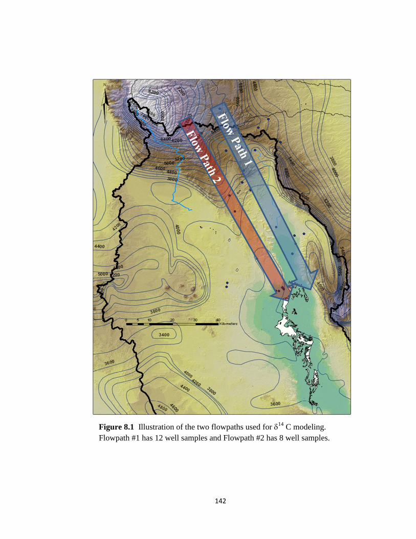
142

Figure 8.1 Illustration of the two flowpaths used for 14

C modeling.

Flowpath #1 has 12 well samples and Flowpath #2 has 8 well samples.

143

y = -1.1137x + 4058.4R² = 0.8885

y = -0.7141x + 2604.1R² = 0.8278

0

20

40

60

80

100

120

140

160

353035403550356035703580359036003610362036303640

Mg

[mg/

L]

Northing [Km]

y = 1.6214x - 5543R² = 0.6173

y = 0.9468x - 3091R² = 0.7216

0

50

100

150

200

250

300

350

400

450

353035403550356035703580359036003610362036303640

HC

O3

[m

g/L]

Northing [Km]

Figure 8.2 ΔMg as a function of distance down the two flowpaths. Linear trends

were used for geochemical modeling with dedolomitization reaction model.

Figure 8.3 ΔHCO3 as a function of distance down the two flowpaths. Linear trends


144

y = -0.0556x + 193.19R² = 0.7527

y = -0.0362x + 122.49R² = 0.7259

-10

-9

-8

-7

-6

-5

-4

-3

-2

-1

0

353035403550356035703580359036003610362036303640

C1

3/C

12

rat

io [

pe

r m

il] P

DB

Northing [Km]

y = 5E-31e0.0204x

R² = 0.8158

0

10

20

30

40

50

60

70

80

90

100

353035403550356035703580359036003610362036303640

C1

4/C

12

rat

io [

pe

r m

il] P

DB

Northing [Km]

Figure 8.4 Carbon-13 as a function of distance down the flow paths. Linear trends


Figure 8.5 Carbon-14 as a function of distance down the flow paths. Linear trends


145

An important model parameter is the isotopic fractionation factor between

bicarbonate and calcite. The Fraction fractor

is temperature dependant as

it is related to equilibrium constants for exchange between the two phases. At

temperatures typical of groundwater in the Salt Basin the isotopic fractionation factor

between bicarbonate and calcite was calculated using Dienes et al. (1974) fractionation

equation. A value of 2.13 was used in the dedolomitization geochemical model.

The 13

C of dolomite is another important factor in the model. Rock cores drilled

into the San Andres formation just east of the study area provided a number (~70) of

stable isotope values for the dolomite unit (Wiggins, 1993). A well constrained value (1σ

± 0.04) of 5.7 per mil was used in the dedolomitization model for the 13

C of dolomite

(13

Cdol).

Section 8.3.c: Final Mass Transfer Results/ Groundwater Age Distribution

The age correction down the flow path is based on sequentially moving along the

continuous-curve fit of the wells calculating the corrected carbon-14 activity (pmcf) and

carbon-13 activity (13

Cf). Starting with initial well on the continuous-curve fit, the

initial carbon-14 activity (pmci) is used in the dedolomitization model to calculate (pmcf)

and (13

Cf) for the first down gradient well. This well then becomes the initial well and

the corrected (pmc) and (13

C) are now used as initial activities in the dedolomitization

model to correct the next down gradient well on the continuous-curve fit, and so on. The

apparent age for each well can then be calculated:

, where -t is the

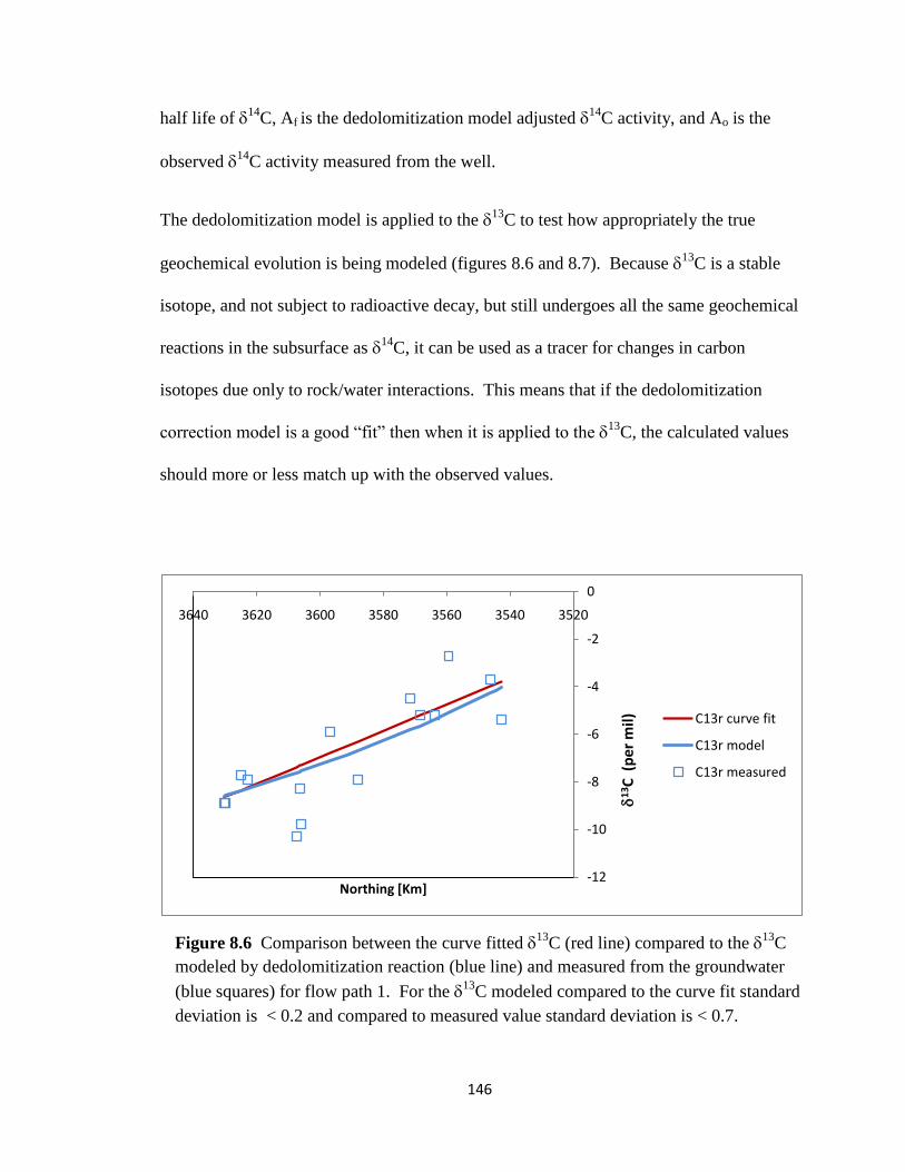
146

half life of 14

C, Af is the dedolomitization model adjusted 14

C activity, and Ao is the

observed 14

C activity measured from the well.

The dedolomitization model is applied to the 13

C to test how appropriately the true

geochemical evolution is being modeled (figures 8.6 and 8.7). Because 13

C is a stable

isotope, and not subject to radioactive decay, but still undergoes all the same geochemical

reactions in the subsurface as 14

C, it can be used as a tracer for changes in carbon

isotopes due only to rock/water interactions. This means that if the dedolomitization

correction model is a good ―fit‖ then when it is applied to the 13

C, the calculated values

should more or less match up with the observed values.

-12

-10

-8

-6

-4

-2

0

3520354035603580360036203640

13C

(p

er

mil

)

Northing [Km]

C13r curve fit

C13r model

C13r measured

Figure 8.6 Comparison between the curve fitted 13

C (red line) compared to the 13

C

modeled by dedolomitization reaction (blue line) and measured from the groundwater

(blue squares) for flow path 1. For the 13

C modeled compared to the curve fit standard

deviation is < 0.2 and compared to measured value standard deviation is < 0.7.

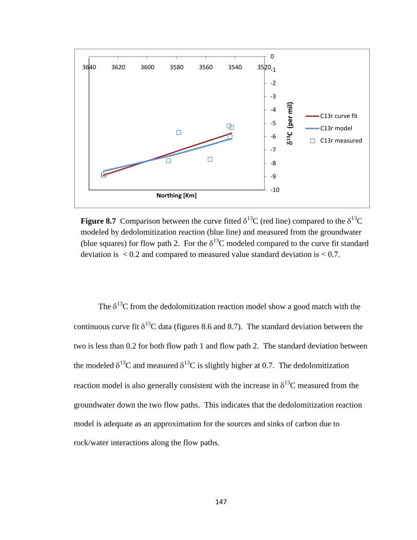
147

The 13

C from the dedolomitization reaction model show a good match with the

continuous curve fit 13

C data (figures 8.6 and 8.7). The standard deviation between the

two is less than 0.2 for both flow path 1 and flow path 2. The standard deviation between

the modeled 13

C and measured 13

C is slightly higher at 0.7. The dedolomitization

reaction model is also generally consistent with the increase in 13

C measured from the

groundwater down the two flow paths. This indicates that the dedolomitization reaction

model is adequate as an approximation for the sources and sinks of carbon due to

rock/water interactions along the flow paths.

-10

-9

-8

-7

-6

-5

-4

-3

-2

-1

0

3520354035603580360036203640

1

3C

(p

er m

il)

Northing [Km]

C13r curve fit

C13r model

C13r measured

Figure 8.7 Comparison between the curve fitted 13

C (red line) compared to the 13

C

modeled by dedolomitization reaction (blue line) and measured from the groundwater

(blue squares) for flow path 2. For the 13

C modeled compared to the curve fit standard

deviation is < 0.2 and compared to measured value standard deviation is < 0.7.

148

Figure 8.8 Distribution of apparent groundwater age in the Salt Basin based

on geochemical modeling using the dedolomitization reaction model. Ages

are expressed in years.

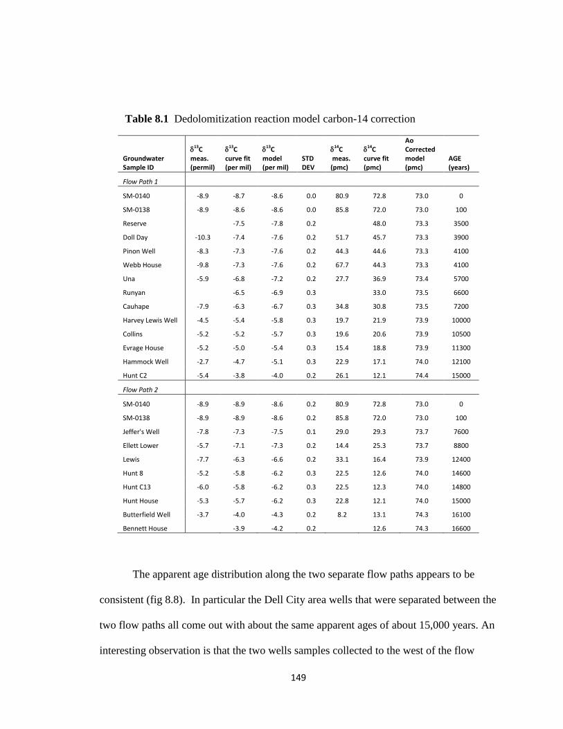
149

Groundwater Sample ID

13C

meas. (permil)

13C

curve fit (per mil)

13C

model (per mil)

STD DEV

14C

meas. (pmc)

14C

curve fit (pmc)

Ao Corrected model (pmc)

AGE (years)

Flow Path 1

SM-0140 -8.9 -8.7 -8.6 0.0 80.9 72.8 73.0 0

SM-0138 -8.9 -8.6 -8.6 0.0 85.8 72.0 73.0 100

Reserve

-7.5 -7.8 0.2

48.0 73.3 3500

Doll Day -10.3 -7.4 -7.6 0.2 51.7 45.7 73.3 3900

Pinon Well -8.3 -7.3 -7.6 0.2 44.3 44.6 73.3 4100

Webb House -9.8 -7.3 -7.6 0.2 67.7 44.3 73.3 4100

Una -5.9 -6.8 -7.2 0.2 27.7 36.9 73.4 5700

Runyan

-6.5 -6.9 0.3

33.0 73.5 6600

Cauhape -7.9 -6.3 -6.7 0.3 34.8 30.8 73.5 7200

Harvey Lewis Well -4.5 -5.4 -5.8 0.3 19.7 21.9 73.9 10000

Collins -5.2 -5.2 -5.7 0.3 19.6 20.6 73.9 10500

Evrage House -5.2 -5.0 -5.4 0.3 15.4 18.8 73.9 11300

Hammock Well -2.7 -4.7 -5.1 0.3 22.9 17.1 74.0 12100

Hunt C2 -5.4 -3.8 -4.0 0.2 26.1 12.1 74.4 15000

Flow Path 2

SM-0140 -8.9 -8.9 -8.6 0.2 80.9 72.8 73.0 0

SM-0138 -8.9 -8.9 -8.6 0.2 85.8 72.0 73.0 100

Jeffer's Well -7.8 -7.3 -7.5 0.1 29.0 29.3 73.7 7600

Ellett Lower -5.7 -7.1 -7.3 0.2 14.4 25.3 73.7 8800

Lewis -7.7 -6.3 -6.6 0.2 33.1 16.4 73.9 12400

Hunt 8 -5.2 -5.8 -6.2 0.3 22.5 12.6 74.0 14600

Hunt C13 -6.0 -5.8 -6.2 0.3 22.5 12.3 74.0 14800

Hunt House -5.3 -5.7 -6.2 0.3 22.8 12.1 74.0 15000

Butterfield Well -3.7 -4.0 -4.3 0.2 8.2 13.1 74.3 16100

Bennett House

-3.9 -4.2 0.2

12.6 74.3 16600

The apparent age distribution along the two separate flow paths appears to be

consistent (fig 8.8). In particular the Dell City area wells that were separated between the

two flow paths all come out with about the same apparent ages of about 15,000 years. An

interesting observation is that the two wells samples collected to the west of the flow

Table 8.1 Dedolomitization reaction model carbon-14 correction

150

paths (Bennett and Butterfield) show the lowest pmc and have the oldest apparent

groundwater age. The presence of old water in this region has implications for whether

or not there is significant recharge from the Cornudas Mountains entering the Salt Basin

graben, as well as what the relative groundwater flux from the western side of the Salt

Basin is compared to the flow paths on the eastern side. The apparent age distribution is

also consistent with the interpretation of 18

O and D, which indicated the presence of

Pleistocene age groundwater in Crow Flats and the Dell City area, implying water ages of

10,000 years old or more.

Section 8.4: Geochemical Modeling using NETPATH

NETPATH (Plummer et al., 1994) is a geochemical model that uses chemical

mass balance, electron balance, and isotope mass balance to define net mass-balance

reactions between an initial and final well along a hydrologic flow path. The program

uses inverse modeling to ascertain the masses (per kilogram of water) of plausible

minerals and gases that must dissolve or precipitate along the flow path to produce the

composition of a selected set of chemical and isotopic observations in the final well. It is

of critical importance that the wells selected truly share common evolution and lie along

well defined flow paths in the aquifer system. The program is exhaustive in that it will

out put any number of models so as to include every possible set of geochemical mass-

balance reactions between the selected evolutionary waters. The better constrained the

flow path and the reactions responsible for the geochemical evolution the more unique

the NETPATH model solution. Given sufficient isotopic data, Rayleigh distillation

calculations can be applied to mass-balance models that satisfy the constraints to predict

changes in isotopic compositions such as carbon. NETPATH is extensively applied to

151

correct radiocarbon ages of groundwater due to geochemical evolution. NETPATH

modeling for radiocarbon dating corrections in the Salt Basin follow examples including

Plummer et al. (1991), Plummer and Hanshaw (1983), and Plummer et al. (1994).

8.4.a: Modeling Strategy for 14

C Mass Transfer in NETPATH

This radiocarbon-dating mass-transfer strategy is laid out in Plummer‘s (1994)

NETPATH Manual. As previously discussed, the adjustment for 14

C needs to account

for two complications that result from aqueous geochemistry: (1) definition of the initial

14

C activity (Ao) in system, (i.e. the recharge zone where the water is isolated from the

modern 14

C reservoir), and (2) adjustment of this initial 14

C activity for geochemical

reactions along the flow path to the final well the 14

C activity has been measured. Many

traditional 14

C adjustment models combine these two problems so that the model can be

applied to a single water analysis at any point in the flow system. NETPATH is different

in that it keeps the two problems separate but requires both initial water and final water

analysis points along an evolutionary flow path. Traditional adjustments are applied only

to the initial water where it will generally be more applicable due to the less complex

geochemical evolution. NETPATH then solves for the mass transfer to pertinent phases

between the initial water and the final down-gradient water. This mass transfer is then

used to adjust the initial 14

C (Ao) for all sources and sinks of carbon that affect the

carbon mass transfer between the two wells. This means at the final well the 14

C

activity is adjusted for geochemical reactions but not radioactive decay, thereby giving

Af. Again, the apparent age is calculated using:

.

152

All carbon leaving the solution between the initial and the final waters, through

carbonate mineral precipitation or outgassing of CO2, is assumed to leave by Rayleigh

distillation processes defined by isotopic fractionation. All carbon mass transfer

associated with minerals or gases that enter the aqueous phase between the initial and

final waters is assumed to enter without isotopic fractionation, and have 13

C and 14

C

(pmc) compositions that are assigned to the specific phases.

The initial water can be represented by any point along the flow path. This

allowed 14

C activity adjustments down flow paths in the Salt Basin to be carried out in

the same fashion as with the dedolomitization model correction. Starting in the recharge

area with the initial well on the flow path, the initial carbon-14 activity (Ao) is used in the

NETPATH model to calculate (Af) for the first down gradient well. This well then

becomes the initial well and the corrected (pmc) is now used as the initial activity (Ao) in

the NETPATH model to correct the next down gradient well, and so on. The modeled

14

C apparent age of the final water, in this case, represents only the travel time between

the initial and final well. To find the actual age of the final water it is necessary to add to

this travel time the age of the initial water.

Section 8.4.b: Selection of Modeling Parameters and Constraints

Flow paths for geochemical modeling in NETPATH to adjust the 14

C activity

from well measurements in the Salt Basin were defined by two main considerations: (1)

the sequence of wells had to be logical relative to groundwater gradients and flow

direction; and (2) initial and final well pairs along a flow path were chosen based on the

best 13

C observed versus measured 1:1 fit. This meant, for example, not all the wells in

153

Crow Flats were interpreted to be evolutionary to one another. If a well pair produced a

very poor 13

C ―fit‖ the initial well was changed to the next nearest up gradient well along

the flow path. Allowing for this kind of spatial variability, as well as NETPATH being

able to account for much more complex geochemical variability compared to the

dedolomitization model, meant that trend lines were not necessary to fit the well

chemistry measurements into the NETPATH model.

In NETPATH phases are defined as any mineral or gas that can enter or leave the

aqueous solution along the evolutionary path. Important phases are defined by the user

and should be based on a predictable geochemical evolution for the flow path. For the

flow paths chosen for geochemical modeling in the Salt Basin, dedolomitization as the

dominant control on the geochemical evolution is well defined. Some phases can

realistically only be precipitated or dissolved, but not both along a flow path. In

NETPATH this is acknowledged and phases can be defined as ―precipitation only‖ or

―dissolution only‖. For the Salt Basin the phases included were dissolution of dolomite,

dissolution of gypsum, precipitation of calcite, as well as, a CO2 phase.

Defining constraints in NETPATH is necessary to determine the extent of the

geochemical reactions. Most constraints are cations and anions typical of aqueous

solutions, but redox states and isotopic elements can also be used. For every phase

defined within NETPATH there must be a constraint associated with it. For the phases

used for geochemical modeling in the Salt Basin, calcium, magnesium, and carbon were

used as constraints. Comparing the observed and calculated 13

C isotopic composition at

the final well can, like the dedolomitization model, be used to interpret how appropriate

the model ―fit‖ is. Because isotopes of 13

C, like 14

C, are involved in carbonate

154

reactions with multiple sources and sinks, it is more appropriately treated using isotope

evolution calculations as opposed to mass balance in NETPATH , in which case it should

not be included as a constraint.

When there is both a source and a sink for an isotope in the reaction, it is treated

as a Rayleigh distillation problem. Isotopic data can be entered for pertinent phases in

the isotopic evolution. The 13

C value for the CO2 of the soil gas was set at -25 per mil,

at value measured from soil gas in the Sacramento Mountains (Morse, 2010). The 13

C

value for dolomite used was the same as for the dedolomitization model, +5.7 per mil

(1σ ± 0.04) measured from the San Andres (Wiggins, 1993). The range of 13

C values

for dolomite from this study measured from about 70 samples is from +4 to +7 per mil.

The 13

C value for calcite used was the average value measured from the San Andres and

Yeso rock samples collected for this study from outcrops in the Sacramento Mountains,

about +2 per mil.

Formation Corrected 13C Std. Dev

San Andres 3.7 0.06

San Andres 2.6 0.07

Yeso 0.4 0.10

The calculated radiocarbon ages are not sensitive to varying the input for the 13

C

values assumed for the carbonate rocks over the two ranges presented above. The main

difference observed in the NETPATH output is the modeled 13

C value. Table 8.3 shows

Table 8.2 13

C values for calcite

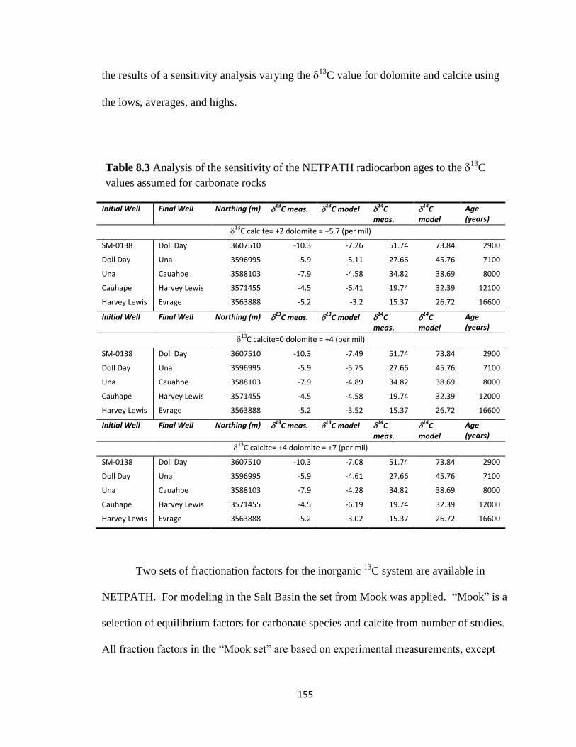
155

the results of a sensitivity analysis varying the 13

C value for dolomite and calcite using

the lows, averages, and highs.

Initial Well Final Well Northing (m) 13

C meas. 13

C model 14

C meas.

14

C model

Age (years)

13

C calcite= +2 dolomite = +5.7 (per mil)

SM-0138 Doll Day 3607510 -10.3 -7.26 51.74 73.84 2900

Doll Day Una 3596995 -5.9 -5.11 27.66 45.76 7100

Una Cauahpe 3588103 -7.9 -4.58 34.82 38.69 8000

Cauhape Harvey Lewis 3571455 -4.5 -6.41 19.74 32.39 12100

Harvey Lewis Evrage 3563888 -5.2 -3.2 15.37 26.72 16600


C meas. 13

C model 14

C meas.

14

C model

Age (years)

13

C calcite=0 dolomite = +4 (per mil)

SM-0138 Doll Day 3607510 -10.3 -7.49 51.74 73.84 2900

Doll Day Una 3596995 -5.9 -5.75 27.66 45.76 7100

Una Cauahpe 3588103 -7.9 -4.89 34.82 38.69 8000




C meas. 13

C model 14

C meas.

14

C model

Age (years)

13

C calcite= +4 dolomite = +7 (per mil)

SM-0138 Doll Day 3607510 -10.3 -7.08 51.74 73.84 2900

Doll Day Una 3596995 -5.9 -4.61 27.66 45.76 7100

Una Cauahpe 3588103 -7.9 -4.28 34.82 38.69 8000



Two sets of fractionation factors for the inorganic 13

C system are available in

NETPATH. For modeling in the Salt Basin the set from Mook was applied. ―Mook‖ is a

selection of equilibrium factors for carbonate species and calcite from number of studies.

All fraction factors in the ―Mook set‖ are based on experimental measurements, except

Table 8.3 Analysis of the sensitivity of the NETPATH radiocarbon ages to the 13

C

values assumed for carbonate rocks

156

for values relating to CO3-2

, which were derived theoretically by Thode and others

(1965). The ―Mook‖ set is given as additive fractionation fractors, εi→j in per mil.

Section 8.4.c: Summary of Final Mass Transfer Results/ Apparent Age Distribution

The phases and constraints used to model the geochemical evolution along flow

paths in the Salt Basin provided a unique solution in NETPATH, in that only one model

was posed to explain the mass transfer. The solution for each well pair along a flow path

defines a balanced chemical reaction and the change in mass for each mineral phase:

Groundwaterinitial + dolomitediss. + gypsumdiss. = Groundwaterfinal - calciteppt

In addition to the solution for the mass balance, NETPATH calculates the isotopic

fractionation associated with the reaction. This allows model calculated 13

C to be

compared to observed 13

C values from the final well and also provides a corrected 14

C

(pmc) and a travel time associated with the distance between the initial and final well.

How well the model calculated 13

C and the observed 13

C ―fit‖ is a check for

how well the true rock/water interactions along the flow path are being model (fig 8.9).

The average standard deviation from the modeled 13

C and the measured 13

C is about

±1.5 per mil. It is interesting to note that the simple dedolomitization model seems to

match the 13

C better (with an average standard deviation of ± 0.7 per mil) than the more

sophisticated NETPATH model. This may be because the generalized trend lines are a

better approximation of the actual flow evolution than the well-to-well comparison.

157

Deviations in 13

C, as well as other evidence of uncertainty in the model such as

precipitation or dissolution inconsistent with saturation indices, may represent modeling

error. There are several possible causes for modeling errors. A significant factor is any

uncertainty in the analytical data. In NETPATH, mass-balance reaction models combine

positive and negative charges in water analyses to compute the masses of uncharged

phases. A consequence is that charge-balance errors can contribute to computed masses

of one-component phases such as CO2. However, CO2 was not found to play a role in

mass transfer in the Salt Basin and so this source of error was likely not a factor. Another

obvious source of uncertainty is in defining the composition of the recharge waters. Even

though modern groundwater in the Sacramento Mountains was relatively well

characterized for this study, uncertainties in 14

C activity from contamination by bomb

-15

-13

-11

-9

-7

-5

-3

-1

1

3

5

35400003560000358000036000003620000

Northing (m)

measured 13Cr

modeled 13Cr

Figure 8.9 Comparison between the observed 13

C compared to the 13

C modeled by

NETPATH as a function of distance along flow path.

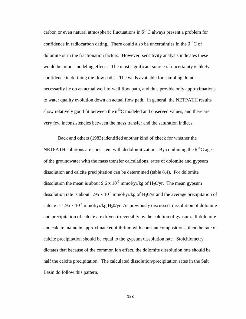
158

carbon or even natural atmospheric fluctuations in 14

C always present a problem for

confidence in radiocarbon dating. There could also be uncertainties in the 13

C of

dolomite or in the fractionation factors. However, sensitivity analysis indicates these

would be minor modeling effects. The most significant source of uncertainty is likely

confidence in defining the flow paths. The wells available for sampling do not

necessarily lie on an actual well-to-well flow path, and thus provide only approximations

to water quality evolution down an actual flow path. In general, the NETPATH results

show relatively good fit between the 13

C modeled and observed values, and there are

very few inconsistencies between the mass transfer and the saturation indices.

Back and others (1983) identified another kind of check for whether the

NETPATH solutions are consistent with dedolomitization. By combining the 14

C ages

of the groundwater with the mass transfer calculations, rates of dolomite and gypsum

dissolution and calcite precipitation can be determined (table 8.4). For dolomite

dissolution the mean is about 9.6 x 10-5

mmol/yr/kg of H20/yr. The mean gypsum

dissolution rate is about 1.95 x 10-4

mmol/yr/kg of H20/yr and the average precipitation of

calcite is 1.95 x 10-4

mmol/yr/kg H20/yr. As previously discussed, dissolution of dolomite

and precipitation of calcite are driven irreversibly by the solution of gypsum. If dolomite

and calcite maintain approximate equilibrium with constant compositions, then the rate of

calcite precipitation should be equal to the gypsum dissolution rate. Stoichiometry

dictates that because of the common ion effect, the dolomite dissolution rate should be

half the calcite precipitation. The calculated dissolution/precipitation rates in the Salt

Basin do follow this pattern.

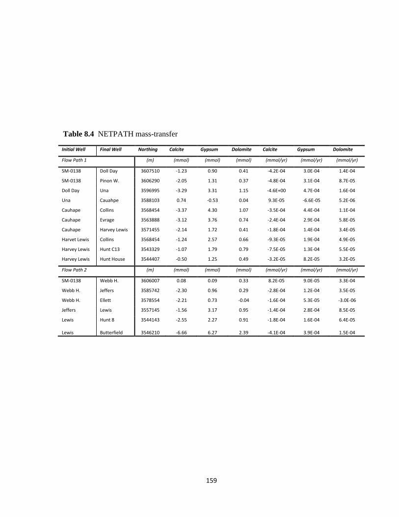
159

Initial Well Final Well Northing Calcite Gypsum Dolomite Calcite Gypsum Dolomite

Flow Path 1 (m) (mmol) (mmol) (mmol) (mmol/yr) (mmol/yr) (mmol/yr)

SM-0138 Doll Day 3607510 -1.23 0.90 0.41 -4.2E-04 3.0E-04 1.4E-04

SM-0138 Pinon W. 3606290 -2.05 1.31 0.37 -4.8E-04 3.1E-04 8.7E-05

Doll Day Una 3596995 -3.29 3.31 1.15 -4.6E+00 4.7E-04 1.6E-04

Una Cauahpe 3588103 0.74 -0.53 0.04 9.3E-05 -6.6E-05 5.2E-06

Cauhape Collins 3568454 -3.37 4.30 1.07 -3.5E-04 4.4E-04 1.1E-04

Cauhape Evrage 3563888 -3.12 3.76 0.74 -2.4E-04 2.9E-04 5.8E-05

Cauhape Harvey Lewis 3571455 -2.14 1.72 0.41 -1.8E-04 1.4E-04 3.4E-05

Harvet Lewis Collins 3568454 -1.24 2.57 0.66 -9.3E-05 1.9E-04 4.9E-05

Harvey Lewis Hunt C13 3543329 -1.07 1.79 0.79 -7.5E-05 1.3E-04 5.5E-05

Harvey Lewis Hunt House 3544407 -0.50 1.25 0.49 -3.2E-05 8.2E-05 3.2E-05

Flow Path 2 (m) (mmol) (mmol) (mmol) (mmol/yr) (mmol/yr) (mmol/yr)

SM-0138 Webb H. 3606007 0.08 0.09 0.33 8.2E-05 9.0E-05 3.3E-04

Webb H. Jeffers 3585742 -2.30 0.96 0.29 -2.8E-04 1.2E-04 3.5E-05

Webb H. Ellett 3578554 -2.21 0.73 -0.04 -1.6E-04 5.3E-05 -3.0E-06

Jeffers Lewis 3557145 -1.56 3.17 0.95 -1.4E-04 2.8E-04 8.5E-05

Lewis Lewis

Hunt 8 Butterfield

3544143

3546210

-2.55

-6.66

2.27

6.27

0.91

2.39

-1.8E-04

-4.1E-04

1.6E-04

3.9E-04

6.4E-05

1.5E-04

Table 8.4 NETPATH mass-transfer

160

The apparent groundwater ages determined using NETPATH are almost identical

to those calculated using the dedolomitization reaction model. Again, there is good

agreement between the two flow paths with the Hunt wells at the distal end of flow paths

1 and 2 all having water ages around 15,000 years. The radiocarbon age determined for

Ellett Well is somewhat anomalous. However, this well has been singled out as an

anomaly in temperature measurement (6.1.a) and chemistry composition (6.2.b) as well.

The difference at this well compared to the regional trend is likely the result of vertical

upwelling due to a localized fault. The two wells west of the main flow path (Bennett

and Butterfield) again show the oldest apparent age.

Initial Well Final Well Northing 13

C meas.

13

C model

d14C meas.

d14C model

Age

Flow Path 1 (m) (per mil) (per mil) (pmc) (pmc) (years)

SM-0138 Doll Day 3607510 -10.30 -7.26 51.74 73.84 2900

SM-0138 Pinon W. 3606290 -8.30 -7.44 73.99 4200

Doll Day Una 3596995 -5.90 -5.11 27.66 45.76 7100

Una Cauahpe 3588103 -7.90 -4.58 34.82 38.69 8000

Cauhape Collins 3568454 -5.20 -3.76 19.62 24.23 9700

Cauhape Evrage 3563888 -5.20 -3.20 15.37 27.53 12800


Harvet Lewis Collins 3568454 -5.20 -2.02 19.62 22.79 13300

Harvey Lewis Hunt C13 3543329 -6.00 -1.64 22.50 25.19 14200

Harvey Lewis Hunt House 3544407 -5.30 -2.52 22.78 29.06 15300

Flow Path 2 (m) (per mil) (per mil) (pmc) (pmc) (years)

SM-0138 Webb H. 3606007 -9.80 -7.27 76.36 1000

Webb H. Jeffers 3585742 -7.80 -8.85 29.04 69.36 8200

Webb H. Ellett 3578554 -5.70 -10.39 14.37 76.90 13800

Jeffers Lewis 3557145 -7.70 -3.96 33.09 47.56 11000

Lewis Lewis

Hunt 8 Butterfield

3544143

3546210

-5.20

-3.70

-4.24

0.026

22.71

8.19

32.29

14.75

14100

16100

Table 8.5 NETPATH radiocarbon correction

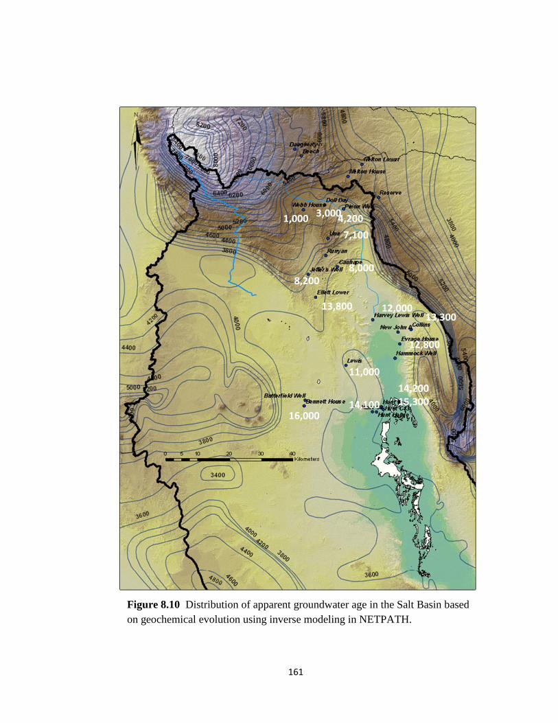
161

Figure 8.10 Distribution of apparent groundwater age in the Salt Basin based

on geochemical evolution using inverse modeling in NETPATH.

162

Section 8.5: Implications for Recharge from Radiocarbon Dating

The apparent age distribution (fig 8.6) based on interpretation of the carbon-14 in

the Salt Basin aquifer system is similar to that of the dedolomitization model. The

groundwater age is an indication of how long a water particle has been in the aquifer

system since recharge. With an understanding of sources of recharge and flow paths, the

groundwater age can be directly related to recharge rates in the Salt Basin. Determining

the extent of recharging fluxes into the Salt Basin groundwater system is a critical

component to proper resource management.

Section 8.5.a: Seepage Velocity/ Hydraulic Conductivity

Along well-defined flow paths apparent water ages can be used to calculate

seepage velocity; seepage velocity (υ) =

. This means the seepage

velocity (υ) is equivalent to the slope in a plot of distance down the flow path versus

groundwater age (fig 8.11). Seepage velocities through the sub-regions of the Salt Basin

(fig 6.1) were calculated (table 8.6).

Region Seepage Velocity () Darcy Velocity (q) Hydraulic Cond. (K) Hydraulic Cond. (K)

(m/yr) (m/yr) (m/y) (m/s) (m/y) (m/s)

ne=8% ne=15% ne=8% ne=8% ne=15% ne=15%

Pinon Area 2.5 0.2 0.4 17.4 5.5E-07 32.7 1.1E-06

Cornucopia Draw 10.2 0.8 1.5 29.7 9.4E-07 29.7 9.7E-07

Crow Flats 8.6 0.7 1.3 294.9 9.4E-06 294.9 9.6E-06

Salt Basin Average 5.1 0.4 0.8 70.3 2.2E-06 131.8 4.3E-06

Table 8.6 Flow velocity and hydraulic conductivity estimated in the Salt Basin

163

Conservative environmental tracers like 14

C move with the water and are thus a

measure of the actual flow velocity or seepage velocity, which is greater than the Darcy

velocity (q) (Swartz and Zhang, 2003). Built into the Darcy velocity is an assumption

that flow occurs over the entire surface area when water really only flows through the

pore space. If the effective porosity (ne) of the aquifer is known or can be accurately

estimated, the Darcy velocity can be calculated (table 8.6) where: .

To the east of the Salt Basin lies the Permian Delaware Basin where dolomite

reservoirs are well known and characterized for their oil production. Porosity and depth

relationships for Permian formations such as the San Andres and Abo have been

evaluated (Galloway, 1983) and can be used as estimates for porosity of the aquifer

Figure 8.11 Distance down the flow path versus groundwater age. The slope through

each sub-region is equivalent to the seepage velocity () m/yr.

164

system in the Salt Basin. Based on the distribution of porosity in these dolomite

reservoirs a range between 8-15% porosity (ne) seems consistent for the San Andres and

Abo formations (fig 8.12). While the Yeso formation is not part of the study,

depositionally it is intermediate between the Abo and the San Andres and would likely

have a similar porosity range.

The hydraulic conductivity (K) can then be calculated using Darcy‘s law where:

q

, and

is the hydraulic gradient (table 8.6). The hydraulic

conductivities calculated along the flow paths in the Salt Basin are within the range

associated with limestone and dolomite commonly reported in the literature (fig 8.13).

The estimates for hydraulic conductivity were also compared to previously reported

Figure 8.12 Plot of average porosity versus depth for major

west Texas oil field (Galloway, 1983)

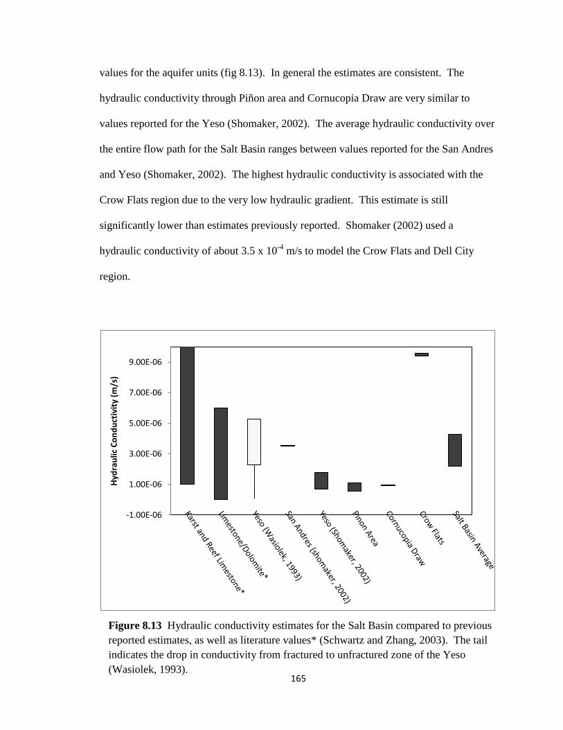
165

values for the aquifer units (fig 8.13). In general the estimates are consistent. The

hydraulic conductivity through Piñon area and Cornucopia Draw are very similar to

values reported for the Yeso (Shomaker, 2002). The average hydraulic conductivity over

the entire flow path for the Salt Basin ranges between values reported for the San Andres

and Yeso (Shomaker, 2002). The highest hydraulic conductivity is associated with the

Crow Flats region due to the very low hydraulic gradient. This estimate is still

significantly lower than estimates previously reported. Shomaker (2002) used a

hydraulic conductivity of about 3.5 x 10-4

m/s to model the Crow Flats and Dell City

region.

-1.00E-06

1.00E-06

3.00E-06

5.00E-06

7.00E-06

9.00E-06

Hyd

rau

lic C

on

du

ctiv

ity

(m/s

)

Figure 8.13 Hydraulic conductivity estimates for the Salt Basin compared to previous

reported estimates, as well as literature values* (Schwartz and Zhang, 2003). The tail

indicates the drop in conductivity from fractured to unfractured zone of the Yeso

(Wasiolek, 1993).

166

Section 8.5.b: Piston-flow Approximation

The trend in groundwater age down the flow path is remarkably consistent with

first order exponential decay associated with carbon-14 radioactive decay. This indicates

that mixing by dispersion/diffusion along the flow path may be relatively insignificant. If

that is the case, the Salt Basin may be appropriately modeled using a simplified

approximation such as piston-flow. With piston-flow (or streamtube) analysis (fig 8.14)

the age (τ) of groundwater is distance (x) to fluid packet‘s point of recharge divided by

distance-averaged flow velocity (υx) (Benthke and Johnson, 2002).

or

Figure 8.14 Piston-flow approximation (Bethke and Johnson, 2002).

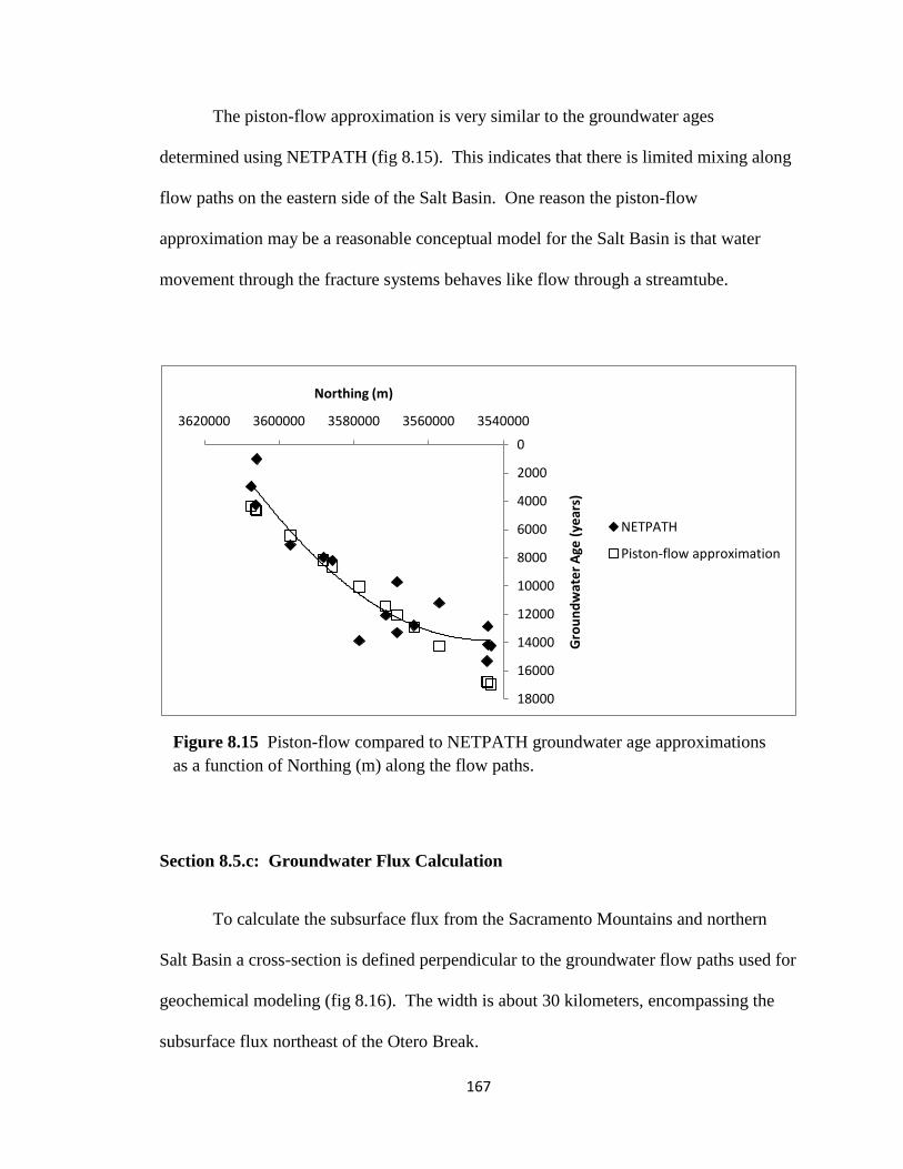
167

The piston-flow approximation is very similar to the groundwater ages

determined using NETPATH (fig 8.15). This indicates that there is limited mixing along

flow paths on the eastern side of the Salt Basin. One reason the piston-flow

approximation may be a reasonable conceptual model for the Salt Basin is that water

movement through the fracture systems behaves like flow through a streamtube.

Section 8.5.c: Groundwater Flux Calculation

To calculate the subsurface flux from the Sacramento Mountains and northern

Salt Basin a cross-section is defined perpendicular to the groundwater flow paths used for

geochemical modeling (fig 8.16). The width is about 30 kilometers, encompassing the

subsurface flux northeast of the Otero Break.

0

2000

4000

6000

8000

10000

12000

14000

16000

18000

35400003560000358000036000003620000

Gro

un

dw

ate

r A

ge (

year

s)

Northing (m)

NETPATH

Piston-flow approximation

Figure 8.15 Piston-flow compared to NETPATH groundwater age approximations

as a function of Northing (m) along the flow paths.

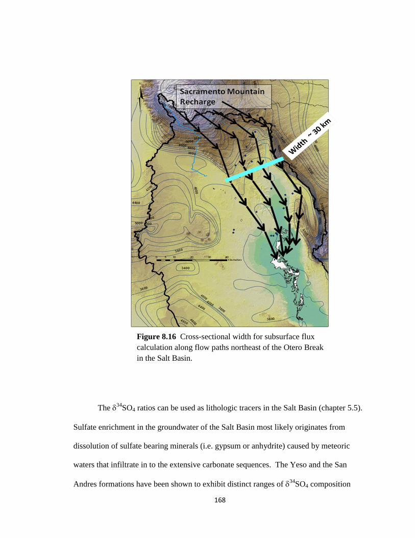
168

The 34

SO4 ratios can be used as lithologic tracers in the Salt Basin (chapter 5.5).

Sulfate enrichment in the groundwater of the Salt Basin most likely originates from

dissolution of sulfate bearing minerals (i.e. gypsum or anhydrite) caused by meteoric

waters that infiltrate in to the extensive carbonate sequences. The Yeso and the San

Andres formations have been shown to exhibit distinct ranges of 34

SO4 composition

Figure 8.16 Cross-sectional width for subsurface flux

calculation along flow paths northeast of the Otero Break

in the Salt Basin.

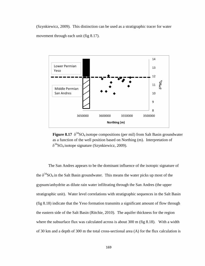
169

(Szynkiewicz, 2009). This distinction can be used as a stratigraphic tracer for water

movement through each unit (fig 8.17).

The San Andres appears to be the dominant influence of the isotopic signature of

the 34

SO4 in the Salt Basin groundwater. This means the water picks up most of the

gypsum/anhydrite as dilute rain water infiltrating through the San Andres (the upper

stratigraphic unit). Water level correlations with stratigraphic sequences in the Salt Basin

(fig 8.18) indicate that the Yeso formation transmits a significant amount of flow through

the eastern side of the Salt Basin (Ritchie, 2010). The aquifer thickness for the region

where the subsurface flux was calculated across is about 300 m (fig 8.18). With a width

of 30 km and a depth of 300 m the total cross-sectional area (A) for the flux calculation is

Figure 8.17 34

SO4 isotope compositions (per mil) from Salt Basin groundwater

as a function of the well position based on Northing (m). Interpretation of

34

SO4 isotope signature (Szynkiewicz, 2009).

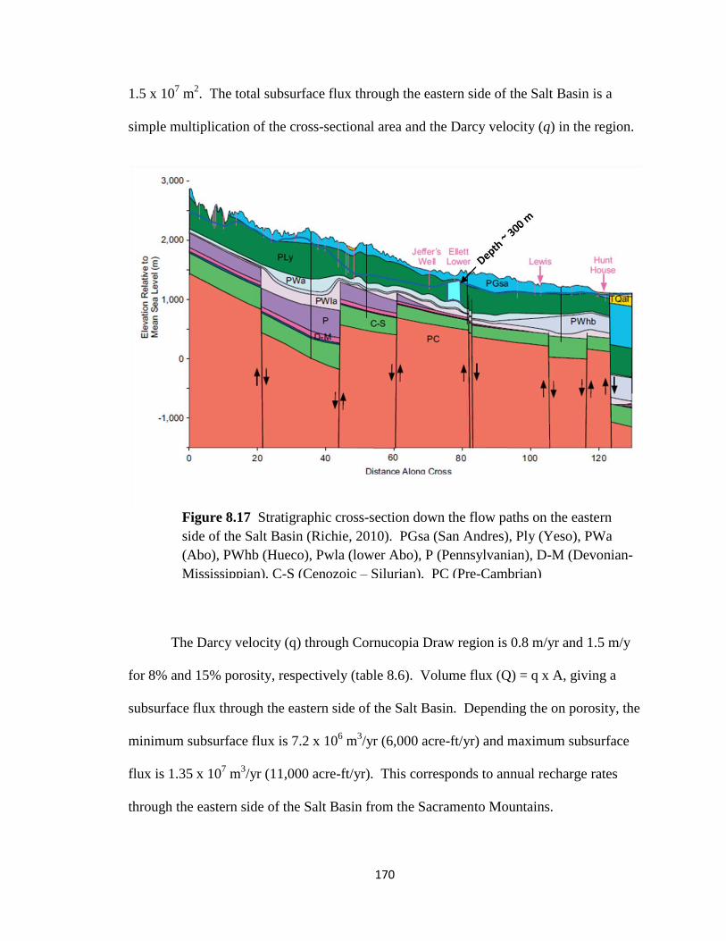
170

1.5 x 107 m

2. The total subsurface flux through the eastern side of the Salt Basin is a

simple multiplication of the cross-sectional area and the Darcy velocity (q) in the region.

The Darcy velocity (q) through Cornucopia Draw region is 0.8 m/yr and 1.5 m/y

for 8% and 15% porosity, respectively (table 8.6). Volume flux (Q) = q x A, giving a

subsurface flux through the eastern side of the Salt Basin. Depending the on porosity, the

minimum subsurface flux is 7.2 x 106 m

3/yr (6,000 acre-ft/yr) and maximum subsurface

flux is 1.35 x 107 m

3/yr (11,000 acre-ft/yr). This corresponds to annual recharge rates

through the eastern side of the Salt Basin from the Sacramento Mountains.

Figure 8.17 Stratigraphic cross-section down the flow paths on the eastern

side of the Salt Basin (Richie, 2010). PGsa (San Andres), Ply (Yeso), PWa

(Abo), PWhb (Hueco), Pwla (lower Abo), P (Pennsylvanian), D-M (Devonian-

Mississippian), C-S (Cenozoic – Silurian), PC (Pre-Cambrian)

171

The presence of additional subsurface fluxes along these flow paths, for instance

from the Guadalupe Mountains, and other hydrodynamics of the system are not explicitly

addressed in the radiocarbon dating model. However, in solving the net mass balance for

water along the flow paths, the introduction or the mixing of water cannot not be

accounted for explicitly and thus any possible contribution from these sources become

incorporated into the overall mass balance solution.

Section 8.5.d: Water Age Correlations with Evolution along Flow Paths

Correlations between magnesium concentration with age (fig 8.19) and sulfate

concentration with age (fig 8.20) confirm that these environmental tracers can be used as

proxies for residence time. The increase in aqueous magnesium and sulfate in the

groundwater is a time-dependant process related to the dissolution of dolomite and

gypsum as the water travels along flow paths. Magnesium is likely the more consistent

tracer because the more evaporitic facies of the Yeso formation under Otero Mesa do

seem to be associated with much higher sulfate concentrations in the groundwater that

may not be a single function of increased residence time.

172

R² = 0.765

0

10

20

30

40

50

60

70

80

90

100

0 2000 4000 6000 8000 10000 12000 14000 16000 18000

Mag

ne

siu

m (

mg/

L)

Groundwater Age (years)

R² = 0.7212

0

100

200

300

400

500

600

700

800

0 2000 4000 6000 8000 10000 12000 14000 16000 18000

Sulf

ate

(m

g/L)

Groundwater Age (years)

Figure 8.20 Solute correlations with NETPATH age for sulfate in the Salt Basin.

Figure 8.19 Solute correlations with NETPATH age for magnesium in the Salt Basin.

173

The correlation between groundwater age and the increase magnesium or sulfate

concentration means that although geochemical modeling with radiocarbon data was only

performed on flow paths on the eastern side of the Salt, the basin-wide distribution of

these constituents (Figures 6.37 and 6.38) have implications for relative fluxes on the

western side of the Salt Basin. For example, flow velocities through the Otero Break do

appear to be higher than those east of the break. However, flow velocities west of the

Otero Break appear to be lower than flow velocities on the eastern side of the Salt Basin.

The groundwater ages from Bennett and Butterfield (just east of the Cornudas

Mountains) are older than any of the wells on the eastern side of the basin. They also lie

within a region of particularly high magnesium and sulfate concentrations (Figures 6.37

and 6.38). The presence of old water in this region has implications for whether or not

there is significant recharge from the Cornudas Mountains entering the Salt Basin graben,

as well as what the relative groundwater flux from the western side of the Salt Basin is

compared to the flow paths on the eastern side.

174

CHAPTER IX

CONCLUSION

Through this geochemical evaluation several characteristics of the Salt Basin

aquifer system were revealed that will play a significant role in future resource

management. Environmental tracers measured from the Salt Basin aquifer system were

used to identify sources recharge, define flow paths, determine the relative amount of

mixing from different sources to the groundwater, identify sources of solutes, and

estimate flow velocities and recharge rates. The use of environmental traces to determine

groundwater ages means that recharge rate and flow velocities can be determined

independently of more traditional aquifer tests. In the Salt Basin the result is likely more

accurate as hydraulic properties of the aquifer are poorly defined and spatially variable.

The present depositional facies and structure of the Salt Basin is the result of a

complex geologic history. Extensive periods of transgression and regression during the

deposition of the Permian aquifer units have led to highly heterogeneous formations.

These were further complicated by subsequent tectonism resulting in regional fault

systems which play a dominant role in groundwater movement in the basin. The

distribution of solutes appears to be strongly correlated with fault zones, which in

addition to elucidating patterns in groundwater flow, highlight regions within the Salt

Basin that are particularly vulnerable in terms of groundwater contamination.

While there are many sources for water entering the Salt Basin graben including

Guadalupe Mountain runoff, distributed recharge throughout the basin from storm event

175

infiltration, as well as, flow across the Diablo Plateau; the main source of recharge is in

the Sacramento Mountains. The water chemistry along the flow path on the eastern side

of the Salt Basin is consistent with groundwater evolution starting in the Sacramento

Mountains and moving south to the Salt Flats near Dell City where it discharges. East of

the Otero Break in the Salt Basin are distinct flow paths along which a complete reaction

series for the dedolomitization process can be observed. This groundwater reaction

involves dissolution and precipitation of carbonate minerals that drive changes in 13

C

and 14

C (Back, 1983). This means that 14

C values measured in the laboratory must be

adjusted to correct for these rock/water interactions for more accurate age estimations.

Along well defined flow paths, groundwater ages can be used to calculate average

seepage velocities and estimate recharge rates.

Radiocarbon dating in the Salt Basin indicates that flow velocities through the

aquifer system are relatively low along the eastern side of the Salt Basin. Flow velocities

(q) range from about 0.5 to 1.5 m/yr. This means that residence times in the Salt Basin

are relatively long. The groundwater ages for the Crow Flats and Dell City regions are

from about 10,000- 15,000 years old. These ages are consistent with the oxygen and

deuterium measured in Crow Flats and Dell City where isotopic signatures indicate

Pleistocene aged recharge.

If the effective porosity of the aquifer is known or can be accurately estimated,

using the seepage velocity the hydraulic conductivity of the aquifer can be easily

estimated. This means across the flow paths on the eastern side of the Salt Basin a

subsurface flux could be determined for the aquifer system over a given thickness. The

subsurface flux gives an estimate of the annual recharge rate to the Salt Basin from the

176

Sacramento Mountains. Porosity was estimated between 8 and 15% based on

observations from the San Andres and Abo formation. The aquifer thickness was

estimated at 300 m through the middle section of the flow path. The subsurface flux or

recharge from the Sacramento Mountains through the eastern side of the Salt Basin

ranges from about 6,000 to 11,000 acre-ft/yr.

The correlation between groundwater age and increase in magnesium or sulfate

concentration in the Salt Basin means that although geochemical modeling with

radiocarbon data was only performed on flow paths on the eastern side of the Salt Basin,

the basin-wide distribution of these constituents have implications for relative fluxes on

the western side of the Salt Basin. Relative to flow through the eastern side of the basin,

flow through the Otero Break appears higher and flow on the western side of the basin

appears slightly lower. Assuming that the flow path on the eastern side of the Salt Basin

constitutes about 1/3 of the total recharge, then a very approximate estimate for total

recharge to the Salt Basin would be about 18,000 to 35,000 acre-ft/yr. Roughly

estimating that the Sacramento Mountains represent about 30 km2 of recharge area with

average precipitation of about 60 cm/yr, then the amount of recharge to the Salt Basin

would constitute about 4% to 8% of the total precipitation.

The estimates for recharge to the Salt Basin from this study fall at the lower end

of the range (~15,000-100,000 acre-ft/yr) presented by the State Engineer‘s Office. They

are also well below the current rate of groundwater pumping (~100,000 acre-ft/yr) in Dell

City. This implies future resource management of the Salt Basin is critically important.

177

REFERENCES

Andrews, J. N., and Lee, D. J. (1979) Inert gases in groundwater from the Bunter Sandstone of

England as indicators of age and paleoclimate trends, Journal of Hydrology, 41, 233-252.

Back, W. (1983) Process and rate of dedolomitization: Mass transfer and 14C dating in a

regional carbonate aquifer, Geological Society of America Bulletin, 94, 1415-

1429.

Back, W. and Hanshaw, B. (1970) Comparison of chemical hydrogeology of the

carbonate peninsulas of Florida and Yucatan, Journal of Hydrology 10, 330-368.

Back, W. and Freeze, R. (1983) Chemical Hydrogeology, Benchmark Papers in Geology-

73, Hutchinson and Ross, Stroudsburg, Pennsylvania.

Bakalowicz, M. (2005) Karst groundwater: A challenge for new resources, Hydrogeology

Journal, 13 (1), 148-160.

Bethke, C., and Johnson, T. (2002) Groundwater age, Groundwater 40, 337-339.

Bjorklund, L. J. (1957) Reconnaissance of Ground-Water Conditions in the Crow Flats Area,

Otero County, New Mexico, State of New Mexico State Engineer Office Technical Report

8, 26.

Black, B. A. (1973) Geology of the Northern and Eastern Parts of the Otero Platform, Otero and

Chaves Counties, New Mexico, University of New Mexico, PhD. Geology, Albuquerque

NM, 170.

178

Black, B. A. (1975) Geology and oil and gas potential of the northeast Otero Platform area, New

Mexico, New Mexico Geological Society Guidebook, 26th Field Conference, Las Cruces

Country ,N.M. Bureau of Mines and Mineral Resources, 323-333.

Black, B. A. (1976) Tectonics of the northern and eastern parts of the Otero Platform, Otero and

Chaves Counties, New Mexico, In Woodward, L. A. and Northrop, S. A. (Eds.),

Tectonics and Mineral Resources in Southwestern North America: New Mexico

Geological Society Special Publication 61, N.M. Bureau of Mines and Mineral

Resources, 39-45.

Bodine, M. W. and Jones, B. F. (1986) THE SALT NORM: A quantitative chemical-

mineralogical characterization of natural waters, U.S. Geological Survey Water

Resources Investigations Report 86-4086, 130.

Boyd, F. M. (1982) Hydrogeology of the Northern Salt Basin of West Texas and New Mexico,

University of Texas, Master of Arts, Austin T.X., 135.

Broadhead, R. F. (2002) Petroleum geology of the McGregor Range, Otero County, New Mexico,

New Mexico Geological Society Guidebook, 53rd

Field Conference, Geology of White

Sands, N.M. Bureau of Mines and Mineral Resources, 331-338.

Brook, G., Folkoff, M., and Box, E. (1983) A world model of soil carbon dioxide, Earth Surface

Processes 8, 79-88.

Buynak, B. (2007) Salt Basin in Water Matters! (2009), The Utton Center Transboundary

Resources, University of New Mexico, N.M., 59-62.

179

Chace, D. A. and Roberts, R. M. (2004) South-central Salt Basin groundwater characterization, El

Paso Geological Society Field Guide Book for the Otero Mesa Area, , New Mexico: El

Paso Geologic Society, 47-61.

Chapman, J. (1984) Hydrogeochemisty of the Unsaturated Zone of a Salt Flat in Hudspeth

County, Texas, University of Texas, Master of Arts, Austin T.X., 132.

Chesterman, C., (1979) National Audubon Society Field Guide to North American Rocks and

Minerals, National Audubon Society, 850-900.

Christophersen, N., and Hooper, R.P. (1992) Multivariate analysis of stream water chemical data:

The use of principal component analysis for the end-member mixing problem, Water

Resources Research, 28 (1), 99-107.

Clark, I., and Fritz, P. (1997) Environmental Isotopes in Hydrogeology, CRC Press LLC, Boca

Raton FL, 198-199.

Coplen, T., Herczeg, A., and Barnes, C. (2000) Isotope engineering-using stable isotopes of the

water molecule to solve practical problems in Environmental Tracers in Subsurface

Hydrology, Cook, P., and Herczeg, A. Kluwer Academic Publishers, Boston, 79-110.

Deines, P., Langmuir, D., and Harmon, R., (1974) Stable carbon isotope ratios and the existence

of a gas phase in the evolution of carbonate groundwaters, Geochim. Cosmochim, Acta.

38, 1147-1164.

Duffy, C.J. (1997) Density-driven groundwater flow in closed desert basins: field investigations

and numerical experiments, Water Resources Research, 196, 139-184.

180

Earman, S., Campbell, A., Phillips, F., Newman, B. (2006) Isotopic exchange between snow and

atmospheric water vapor: Estimation of the snowmelt component of groundwater

recharge in the southwestern United States, Journal of Geophysical Research 111,

D09302, doi:10.1029/2005JD006470

Eastoe, C. J. (2002) Isotopes in the Hueco Bolson Aquifer, Texas (USA) and Chihuahua

(Mexico): local and general implications for recharge sources in alluvial basins,

Hydrogeology Journal 16 (4), 737-747.

Edmunds, W., Smedley, P. (1999) Residence time indicators in groundwater; the East Midlands

Triassic Sandstone aquifer, Applied Geochemistry 15, 737-752.

Edmunds, W., Cook, J., Kinniburgh, D., Miles, D., Bath, A., Morgan-Jones M., and Andrews, J.

(1987) Baseline geochemical conditions in the chalk aquifer, Bershire UK: a basis for

groundwater quality management, Applied Geochemistry 2, 251-274.

Eugster, H. P. (1978) Saline lakes, Chemistry, Geology, and Physics ed. A. Lerman, Springer

N.Y., 237-293.

Finch, S. T., Jr. (2002) Hydrogeologic Framework of the Salt Basin and Development of Three-

Dimensional Ground-Water Flow Model, John Shomaker & Associates, Inc. Final

Report, Prepared for New Mexico Interstate Stream Commission, 28 p.

Fritz, P., and Fontes, J., (1980) Handbook of Environmental Isotope Geochemistry (vol 1), the

Terrestrial Environment, Elsevier, Amsterdam, 545.

181

Galloway, W., Ewing T., Garrett Jr. C., Tyler N., and. Bebout D. (1983) Atlas of major Texas oil

reservoirs, University of Texas, Austin, Bureau of Economic Geology

Special Publication, 139.

Gat, J.R (1980) The isotopes of hydrogen and oxygen in precipitation in Handbook of

Environmental Isotope Geochemistry (vol 1), Fritz, P., and Fontes, J., Elsevier,

Amsterdam, 21-47.

Gibbard, P., Head, M., Walker, M., and the Subcommission on Quaternary Stratigraphy (2009)

Formal ratification of the Quaternary System/Period and the Pleistocene Series/Epoch

with a base at 2.58 Ma., Journal of Quaternary Science, DOI: 10.1002/jqs.1338

Godwin, H. (1962) Half-life of radiocarbon, Nature 195 (4845), 984.

Goetz, L. K. (1977) Quaternary Faulting in the Salt Basin Graben, West Texas, University of

Texas, Master of Arts, Austin, T.X., 136 p.

Goetz, L. K. (1980) Quaternary faulting in Salt Basin graben, West Texas, New Mexico

Geological Society Guidebook, 31st Field Conference, Trans-Pecos Region, N.M. Bureau

of Mines and Mineral Resources, 83-92.

Goetz, L. K. (1985) Salt Basin graben: A basin-and-range right-lateral transtensional fault zone,

some speculations, In Dickerson, P. W. and Muehlberger, R. W. (Eds.), Structure and

Tectonics of Trans-Pecos Texas: West Texas Geological Society Publication 85-81,

Midland T.X., 165-168.

182

Hanshaw B. B. (1971) A geochemical hypothesis for dolomitization by groundwater, Economic

Geology, 66(5), 710-724.

Herczeg, A., Edmunds, M. (2000) Inorganic ions as tracers in Environmental Tracers in

Subsurface Hydrology, Cook, P., and Herczeg, A., Kluwer Academic Publishers, Boston,

31-78.

Hooper, R.P. (2003) Diagnostic tools for mixing models of stream water chemistry, Water

Resources Research, 39 (3), 1055-1068.

Huff, G. F. and Chace, D. A. (2006) Knowledge and understanding of the hydrogeology of the

Salt Basin in south-central New Mexico and future study needs, U.S. Geological Survey

Open-File Report 2006-1358, 17.

Ingraham, N.L. (1990) Stable isotopes in cave pool systems: Carlsbad Cavern, New Mexico,

U.S.A., Chemical Geology, 86, 65-75.

Kalin, R. (2000) Radiocarbon dating groundwater systems in Environmental Tracers in

Subsurface Hydrology, Cook, P., and Herczeg, A., Kluwer Academic Publisher,

Boston,111-143.

Kaufman, S., and Libby, W. F. (1954) The natural distribution of tritium, Physics Review, 93,

1337-1344.

Kelley, V. C. (1971) Geology of the Pecos Country, Southeastern New Mexico, New Mexico

Bureau of Mines & Mineral Resources Memoir 24, Socorro N.M., 75.

183

King, P. B. (1948) Geology of the Southern Guadalupe Mountains, Texas, U.S. Geological

Survey Professional Paper 215, 183.

King, P. B. (1965) Geology of the Sierra Diablo Region Texas, U.S. Geological Survey

Professional Paper 480, 185.

King, P. B. (1983) Leonard and Wolfcamp Series of Sierra Diablo, Texas, In Meader-Roberts, S.

J. (Eds.), Geology of the Sierra Diablo and Southern Hueco Mountains West Texas:

Permian Basin Section Society of Economic Paleontologists and Mineralogists Field

Conference Guidebook 83-22, T.X., 80-96.

King, P. B., King, R. E., and Knight, J. B. (1945) Geology of the Hueco Mountains, El Paso and

Hudspeth Counties, U.S. Geological Survey Oil and Gas Inv. Prelim. Map, 36, 2 sheets.

King, W. E. and Harder, V. M. (1985) Oil and Gas Potential of the Tularosa Basin-Otero

Platform-Salt Basin Graben Area, New Mexico and Texas, New Mexico Bureau of Mines

and Mineral Resources Circular 198, Socorro, N.M., 36 p.

Kreitler, C. W., Mullican, W. F., and Nativ, R. (1990) Hydrogeology of the Diablo

Plateau, Trans-Pecos Texas, In Kreitler, C. W. and Sharp, J. M., Jr. (Eds.),

Hydrology of Trans-Pecos Texas: Texas Bureau of Economic Geology Guidebook

25,T.X., 49-58.

Krouse, R., and Mayer, B. (2000) Sulphur and oxygen isotopes in sulphate in

Environmental Tracers in Subsurface Hydrology, Cook, P., and Herczeg, A.,

Kluwer Academic Publisher, Boston, 195-232.

184

Langmuir, D. (1997) Aqueous Environmental Geochemistry, Prentice Hall, U.S.A., 30-

74.

Loaiciga, H., (2004) Residence time, groundwater age, and solute output in steady-state

groundwater systems, Advances in Water Resources 27, 681-688

Liu, F., Williams, M.W. (2004) Source water and flow paths in an alpine catchment, Colorado

Front Range, U.S.A., Water Resources Research, 40, 9401.

Liu, F., Bales, R., Conklin M., and Conrad M. (2008) Streamflow generation from snowmelt in

semi-arid, seasonally snow-covered, forested catchments, Valles Caldera, New Mexico,

Water Resources Research, 44. doi:10.1029/2007WR006728

Mayer, J. R. (1995) The Role of Fractures in Regional Groundwater Flow: Field Evidence and

Model Results from the Basin-and-Range of Texas and New Mexico, University of

Texas, PhD., Austin, T.X., 218.

Mayer, J. R. and Sharp, J. M., Jr. (1995) The role of fractures in regional groundwater flow, in

Rossmanith, H. (Eds.), Mechanics of Jointed and Faulted Rock, U.S.A., 375-380.

Mayer, J. R. and Sharp, J. M., Jr. (1998) Fracture control of regional ground-water flow in a

carbonate aquifer in a semi-arid region, Geological Society of America Bulletin, 110(2),

269–283.

Mazzullo, S.J. (1995) Permian stratigraphy and facies, Permian basin (Texas-New Mexico) and

adjoining areas in the Midcontinent United States, in Scholle, P., Peryt, T., and Ulmer-

185

Scholle, D., eds., The Permian of Northern Pangea (vol 2), Sedimentary Basins and

Economic Resources,Spring-Verlag, N.Y.,41-60.

McGuire, K., and McDonnell, J., (2006) A review and evaluation of catchment transit time

modeling, Journal of Hydrology 330, 543-563.

Milner, S. (1976) Carbonate petrology and syndepositional facies of the lower San Andres

formation (middle Permian), Lincoln County, NM, Journal of Sedimentary Petrology,

46( 3) , 463-482.

Mook, W., and van de Plicht, J. (1999) Reporting 14C activities and concentrations, Radiocarbon

41, 227-239.

Muehlberger, W. R., Belcher, R. C., and Goetz, L. K. (1978) Quaternary faulting in Trans-Pecos

Texas, Geology, 6, 337-340.

Muir, N.J. (1978) Depositional Environments and Diagenesis of the Lower San Andres

Formation, Roosevelt and Quay Counties, New Mexico, Texas Tech University, PhD.,

Lubbock, T.X., 68.

National Elevation Dataset: USGS, 2009, www.ned.usgs.gov/

National Hydrography Dataset: USGS, 2010, www.nhd.usgs.gov/

Nelson, S.T., and Dettman, D. (2001) Improving hydrogen isotope ratio measurements for on-line

chromium reduction systems, Rapid Communications in Mass Spectrometry 15, 1751-

1753.

186

Nutt, C. J., O‘Neill, J. M., Kleinkopf, M. D., Klein, D. P., Miller, W. R., Rodriquez, B. D., and

McLemore, V. T. (1997) Geology and Mineral Resources of the Cornudas Mountains,

New Mexico, U.S. Geological Survey Open-File Report 97-282, 46 p.

Phillips, F., Peeters, L., Tansey, M., and Davis, S. (1986) Paleoclimate inferences from an

isotopic investigation of ground water in the central San Juan Basin, New Mexico,

Quaternary Research 26, 179-192.

Plummer, L. N. (1991) Geochemical evolution of water in the Madison Aquifer in parts of

Montana, South Dakota, and Wyoming, U.S. Geological Survey Professional Paper,

1273-F.

Plummer, L. N. (1994) An interactive code (NETPATH) for modeling net geochemical reactions

along a flow path- version 2.0, USGS Water Resources Investigation Report, 94-4169.

Rawling, G., Newton, T., Timmons, S., Partey, F., Kludt, T., Land, L., Timmons, M., Walsh, P.,

(2008) Sacramento Mountain hydrogeology study, NM Bureau of Geology and Mineral

Resources 518, Socorro, N.M., 11-53.

Reiter, M., and Jordan, D. (1996) Hydrogeothermal studies across the Pecos River Valley,

southeastern New Mexico, Geological Society of America Bulletin 108, 747-756.

Ritchie, A., (2010) Hydrogeologic Framework and Development of a 3-D Finite Difference

Groundwater Flow Model of the Salt Basin, New Mexico and Texas, Master of Science,

New Mexico Institute of Mining and Technology, Socorro, N.M.

187

Ross, C.A. (1986) Paleozoic evolution of southern margin of Permian basin, Geologic Society of

America Bulletin 97, 536-554.

Rozanski, K., Araguau-Araguas, L, and Confiantini, R., (1993) Isotopic patterns in modern global

precipitation in Climate Change in Continental Isotopic Records, Stwart, P., Lohmann,

K., McKenzi, J., and Savin, S., American Geophysical Union, Geophysical Mongraph 78,

1-36.

Rozanski, K., Johnsen, S. J., Schotterer, U., and Thompson, L. G. (1997) Reconstruction of past

climates from stable isotope records of palaeo-precipitation preserved in continental

archives, Hydrologic Sciences- Journal-des Sciences Hydrologiques, 42, 725-729.

Scalapino, R. A. (1950) Development of groundwater for irrigation in the Dell City Area,

Hudspeth County, Texas, Texas Board of Water Engineers Bulletin 5004, T.X., 38 p.

Sharp, J. M., Jr. (1989) Regional ground-water systems in northern Trans-Pecos Texas, In

Dickerson, P. W., and Muehlberger, W. R. (Eds.), Structure and Stratigraphy of Trans-

Pecos Texas: American Geophysical Union Field Trip Guidebook T317, U.S.A., 123-130.

Sharp, J. M., Jr. (2001) Regional groundwater glow systems in Trans-Pecos Texas, In Mace, R.

E., Mullican, W. F. III, and Angle, E. S. (Eds.), Aquifers of West Texas: Texas Water

Development Board Report 356, T.X., 41-75.

Sharp, J. M., Jr., Mayer, J. R., and McCutcheon, E. (1993) Hydrogeologic Trends in the Dell City

area, Hudspeth County, Texas, New Mexico Geological Society Guidebook, 44th Field

Conference, N.M. Bureau of Mines and Mineral Resources, Carlsbad, 327-330.

188

Sharp, Z. (2007) Principles of stable isotope geochemistry, Prentice Hall, 65-100 p.

Solomon, D., and Cook, P. (2000) 3H and

3He in Environmental Tracers in Subsurface

Hydrology, Cook, P. and Herczeg, A., Kluwer Academic Publisher, Boston, 397-424.

Stoeser, D. B., Green, G. N., Morath, L. C., Heran, W. D., Wilson, A. B., Moore, D. W.,

and Van Gosen, B. S. (2007) Preliminary Integrated Geologic Map Databases for

the United States: Central States: Montana, Wyoming, Colorado, New Mexico,

North Dakota, South Dakota, Nebraska, Kansas, Oklahoma, Texas, Iowa,

Missouri, Arkansas, and Louisiana, U.S. Geological Survey Open-File Report,

2005-1351, Version 1.2. http://pubs.usgs.gov/of/2005/1351/.

Stute, M., Clark, J., Schlosser, P., Broecker, W., and Bonani, G. (1995) A 30,000 yr

continental paleotemperature record derived from noble gases dissolved in

groundwater from the San Juan Basin, New Mexico, Quaternary Research 43,

209-220.

Stuiver, M., and Polach, H. (1977) Discussion—reporting of 14

C Data, Radiocarbon 19

(3), 355-363.

Szynkiewicz, A. (2009) Sulfur isotope signatures in gypsiferous sediments of the Estancia and

Tularosa Basin as indicators of sulfate sources, hydrologic processes, and microbial

actvitity, Geochimica et Cosmochimica acta 73, M.O., 6162-6186.

http://pubs.usgs.gov/of/2005/1351/

189

Tillery, A. (2010) Estimates of mean annual flow and flow loss for ephemeral channels in the Salt

Basin, southern New Mexico, United States Geologic Survey, Scientific Investigation

Report 2010-XXXX, Virginia, 12-19.

Uliana, M. M. (2000) Delineation of Regional Groundwater Flow Paths and their Relation to

Structural Features in the Salt and Toyah Basins, Trans-Pecos Texas, University of Texas,

Ph.D., Austin, T.X., 215.

Uliana, M. M. (2001) The Geology and hydrogeology of the Capitan Aquifer: A brief overview,

In Mace, R. E., Mullican, W. F. III, and Angle, E. S. (Eds.), Aquifers of West Texas:

Texas Water Development Board Report 356, U.S.A., 153-166.

Uliana, M. M. and Sharp, J. M., Jr. (2001) Tracing regional flow paths to major springs in Trans-

Pecos Texas using geochemical data and geochemical models, Chemical Geology, 179,

U.S.A., 53-72.

Uliana, M. M., Banner, J. L., and Sharp, J. M., Jr. (2007) Regional groundwater flow paths in

Trans-Pecos, Texas inferred from oxygen, hydrogen, and strontium isotopes, Journal of

Hydrology 334, U.S.A, 334-346.

Unterweger, M., Coursey, B., Schima, F., and Mann, W., (1980) Preparation and calibration of

the 1978 national bureau of standards tritiated-water standards, International Journal of

Applied Radioactive Isotopes 31, 611-614.

United States Census Bureau, 2010, www.census.gov/

United States Department of Agriculture, 2010, www.usda.gov/

http://www.usda.gov/

190

United States Geologic Survey, 2009, Data: obtained from water-streamflow

www.water.usgs.gov/

United States Environmental Protection Agency, 2010, www.epa.gov/

Vogel, J.C. and D. Ehhalt (1963), The use of carbon isotopes in groundwater studies,

Radioisotopes in Hydrology, International Atomic Energy Agency, Vienna, 383-

395.

Vogel, J.C. (1967), Investigation of groundwater flow with radiocarbon, Isotopes in

Hydrology, International Atomic Energy Agency, Vienna, 355-368.

Vogel, J.C. (1970), Carbon-14 dating of groundwater, Isotope Hydrology 1970,

International Atomic Energy Agency, Vienna, 235-237.

Wasiolek, M., (1991) The hydrogeoly of the Permian Yeso Formation within the Upper Rio

Hondo Basin and the eastern Mescalero Apache Indian Reservation, Lincoln and Otero

Counties New Mexico, New Geologic Society Guidebook, N.M. Bureau of Mines and

Mineral Resources, Socorro, N.M., 343-351.

Wiggins, W. D. (1993) Geochemistry of Post-uplift Calcite in the Permian Basin of Texas and

New Mexico, Geological Society of American Bulletin779-790.

Yonge, C. J. (1985) Stable isotope studies of cave seepage water, Chemical Geology (Isotope

Geoscience Section), 58, 97-105.

http://www.epa.gov/

APPPENDICES

Appendix A. Analytical Chemistry from the Salt Basin Groundwater Samples

Collected 2008—2009 (Andre Ritchie and Sophia Sigstedt)

Appendix B. General Chemistry from the Sacramento Mountains Groundwater

Source: New Mexico Bureau of Geology and Mineral Resources

Appendix C. Compiled General Chemistry from Groundwater in the Salt Basin

Source: Mayer, 1995

ABSTRACT

The Salt Basin was declared by the New Mexico State Engineer in 2000,

estimates for recharge reported vary anywhere from 20,000 to 100,000 acre-ft/yr. In

addition to local demands on water for agricultural purposes, interest has arisen in the

groundwater resources of the Salt Basin as a future source of water for a number of

competing groundwater appropriations bids. Thus, long-term management of the water

resources is needed. In order to inform long-term management strategies, this study seeks

to establish a conceptual model of groundwater flow in the Salt Basin.

An adequate conceptual model of groundwater flow in the Salt Basin relies on the

development of a hydrogeologic framework, which involves reconstructing the tectonic

forcings that have affected the basin during its formation, and identifying the depositional

environments that formed and the resultant distribution of facies. The distribution of

facies and structural features can then be used to evaluate the distribution of permeability

within the basin, and conceptualize the groundwater flow system. The aquifer system is

further characterized using a suite of environmental tracers to identify sources of

recharge, estimates of recharge rate, flowpaths and directions, flow rates, and sources of

solutes in the groundwater. This information is critical for determining volumetric fluxes

and estimates for the amount of available water in the Salt Basin.

ENVIRONMENTAL TRACERS IN GROUNDWATER ... TRACERS IN GROUNDWATER OF THE SALT BASIN, NEW MEXICO, AND...

Documents

Transcript of ENVIRONMENTAL TRACERS IN GROUNDWATER ... TRACERS IN GROUNDWATER OF THE SALT BASIN, NEW MEXICO, AND...