ENVIRONMENTAL REACTION KINETICS Lecture #18 REACTION KINETICS David A. Reckhow Introduction ... No...

11/13/2013

1

CEE 697KENVIRONMENTAL REACTION KINETICS

IntroductionDavid A. Reckhow

CEE 679 Kinetics Lecture #18 1Updated: 13 November 2013

Print version

Lecture #18

Chloramines with Surface Reactions: Pipe walls & degradation in Distribution SystemsPrimary Literature

H2OH2O

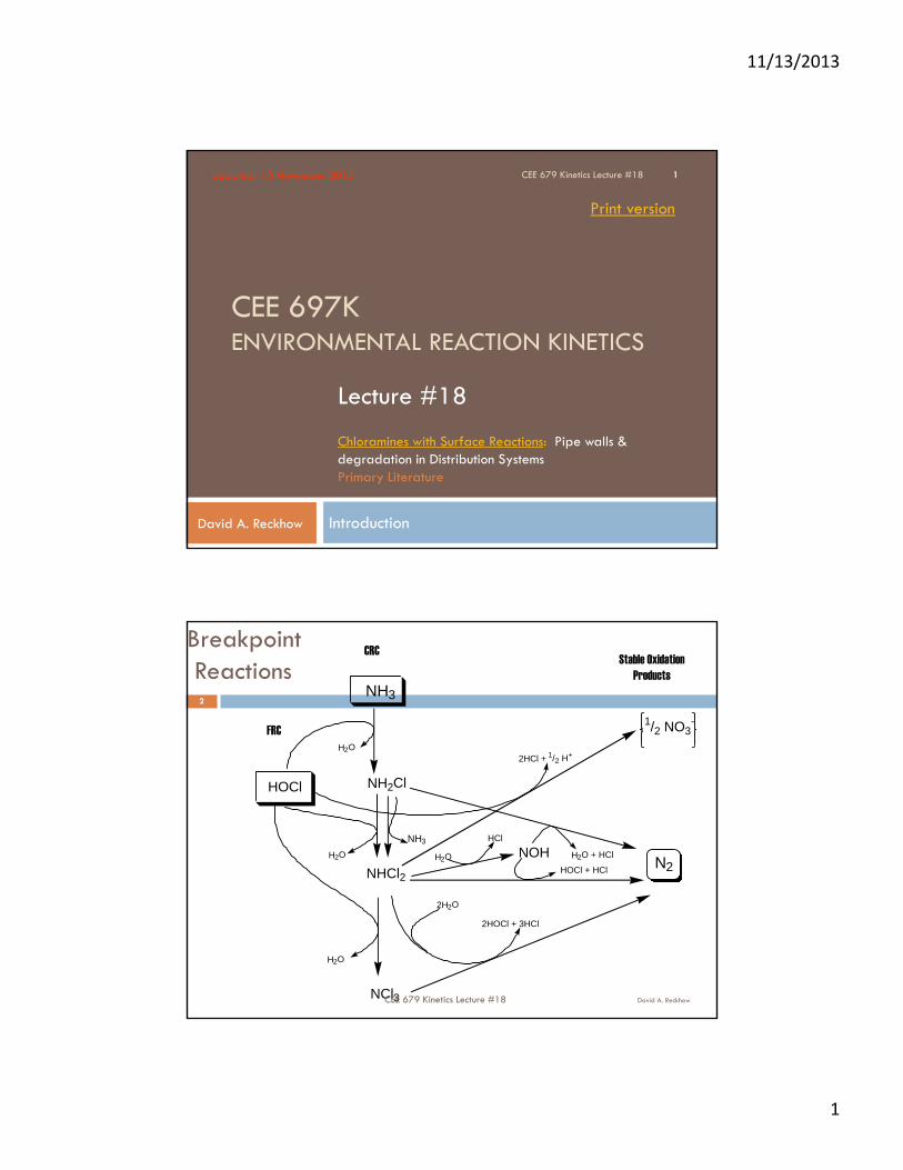
NH3

NCl3

NH2ClHOCl

NOH

NHCl2

H2O

H2O

2H2O

1/2 NO3-

2HCl + 1/2 H+

N2H2O + HCl

HOCl + HCl

HCl

2HOCl + 3HCl

NH3

BreakpointReactions

Stable OxidationProducts

FRC

CRC

David A. ReckhowCEE 679 Kinetics Lecture #18

2

11/13/2013

2

Statistics


3

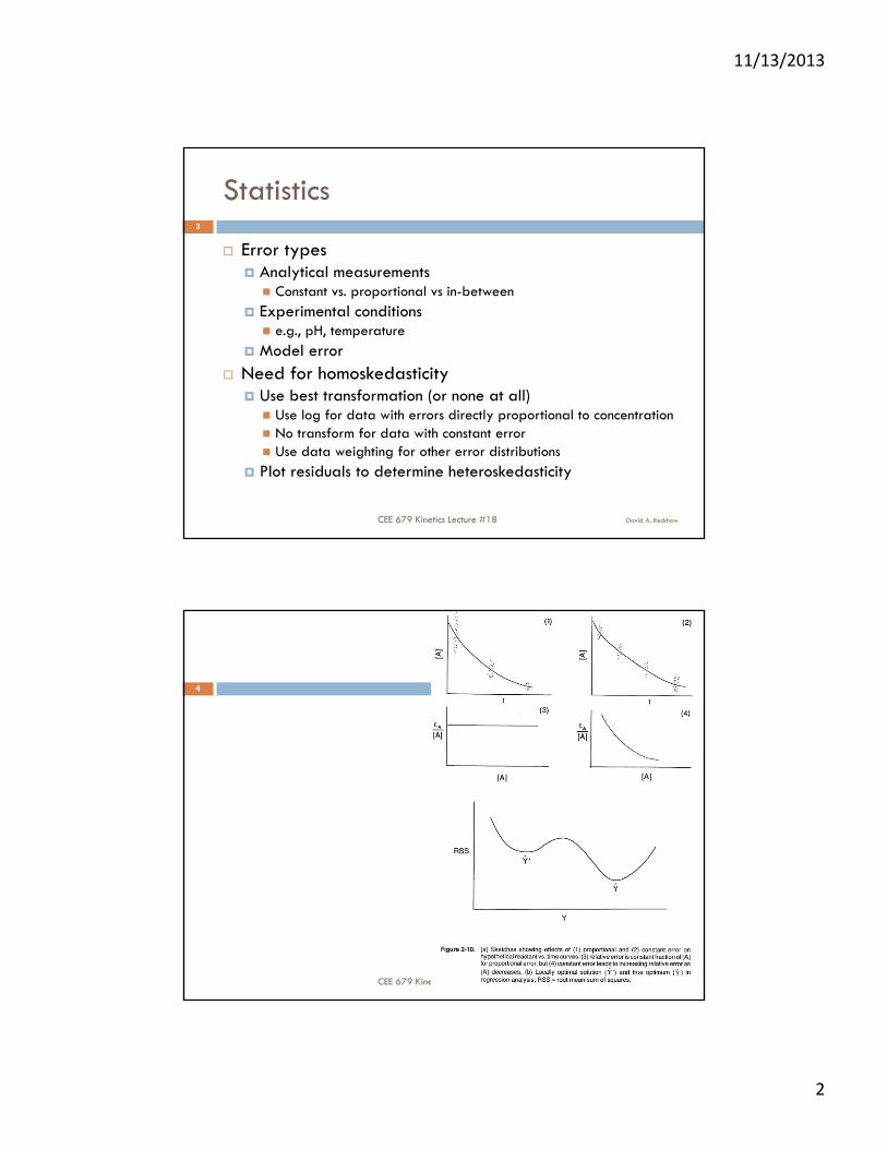
Error types Analytical measurements Constant vs. proportional vs in-between

Experimental conditions e.g., pH, temperature

Model error Need for homoskedasticity

Use best transformation (or none at all) Use log for data with errors directly proportional to concentration No transform for data with constant error Use data weighting for other error distributions

Plot residuals to determine heteroskedasticity


4

11/13/2013

3

Kinetic Spectrum Analysis


5

For mixtures of many closely related compounds A new continuum of rate constants E.g., NOM

Kinetic: Shuman model

Equilibria: Perdue model

Very general, but highly subject to errors

n

i

tkit

ieCC1

0][][

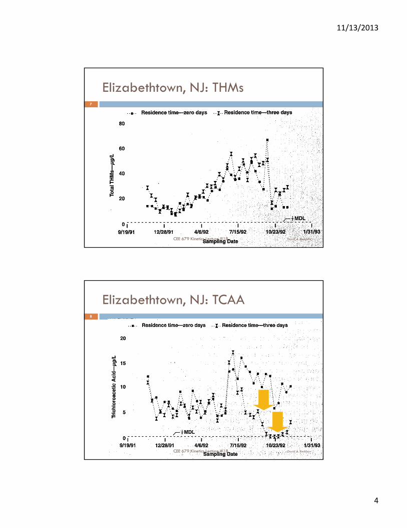
Seasonal Variability & Biodegradation6

Chen & Weisel study

JAWWA, April 1998

Intensive study of Elizabethtown, NJ system 125 MGD conventional plant

4.9 mg/L DOC (raw water average)

pH 7.2


11/13/2013

4

Elizabethtown, NJ: THMs7


Elizabethtown, NJ: TCAA8


11/13/2013

5

HAA Degradation9

Biodegradation:

dihaloacetic acids degrade more readily than trihaloacetic acids

On BACMHAA>DHAA>THAA

Wu & Xie, 2005 [JAWWA 97:11:94]

In distribution systems DHAA>MHAA>THAA

Many studies


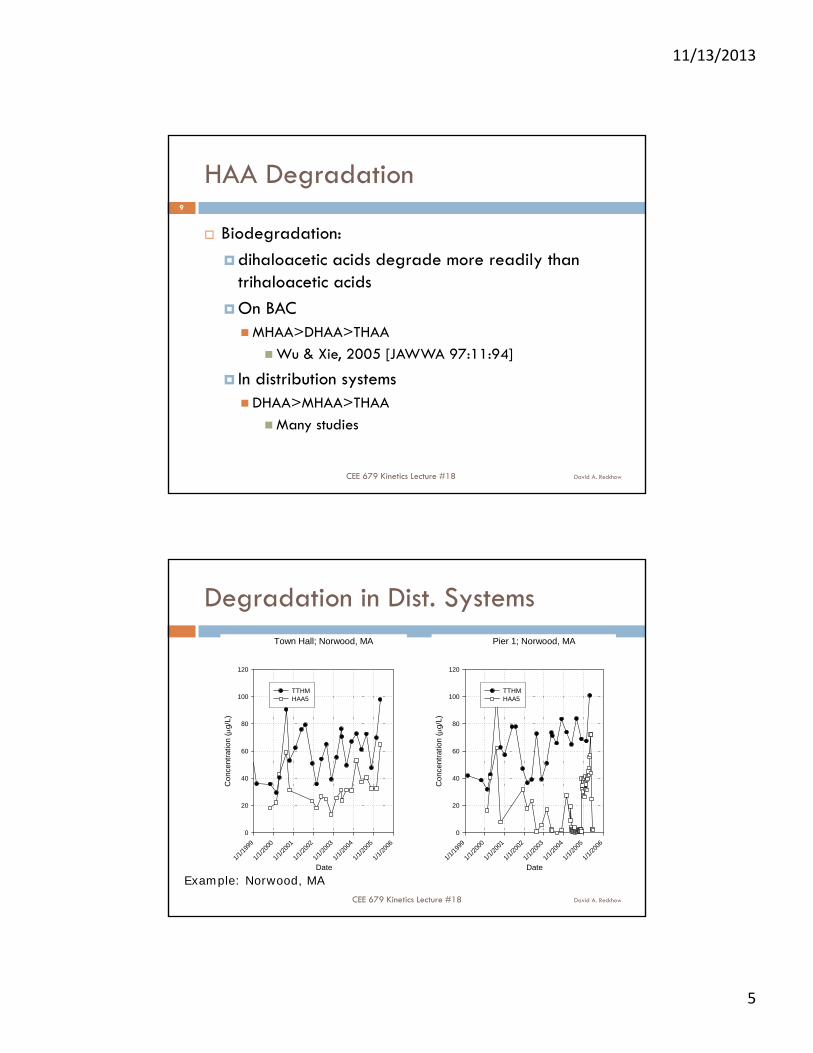
Degradation in Dist. Systems

10

Town Hall; Norwood, MA

Date1/

1/19

99

1/1/

2000

1/1/

2001

1/1/

2002

1/1/

2003

1/1/

2004

1/1/

2005

1/1/

2006

Co

ncen

trat

ion

(g/

L)

0

20

40

60

80

100

120

TTHMHAA5

Pier 1; Norwood, MA

Date1/

1/19

99

1/1/

2000

1/1/

2001

1/1/

2002

1/1/

2003

1/1/

2004

1/1/

2005

1/1/

2006

Co

ncen

trat

ion

(g/

L)

0

20

40

60

80

100

120

TTHMHAA5

Example: Norwood, MADavid A. ReckhowCEE 679 Kinetics Lecture #18

11/13/2013

6

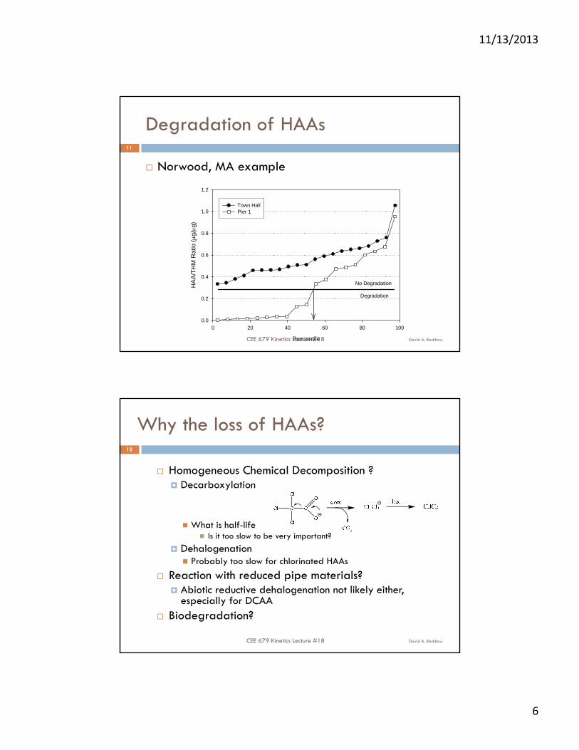
Degradation of HAAs11

Norwood, MA example

Percentile

0 20 40 60 80 100

HA

A/T

HM

Rat

io ( g

/g)

0.0

0.2

0.4

0.6

0.8

1.0

1.2

Town HallPier 1

No Degradation

Degradation


Why the loss of HAAs?

Homogeneous Chemical Decomposition ? Decarboxylation

What is half-life Is it too slow to be very important?

Dehalogenation Probably too slow for chlorinated HAAs

Reaction with reduced pipe materials? Abiotic reductive dehalogenation not likely either,

especially for DCAA Biodegradation?

12


11/13/2013

7

A few recent studies


13

Modeling HAA Biodegradation in Biofilters and Distribution Systems Alina S. Grigorescu and Ray Hozalski, University of

Minnesota at Minneapolis

Journal AWWA, July 2010, 102(7)67-80

Background conclusion?

“Thus aerobic biodegradation is believed to be the dominant HAA degradation process in ….…..water distribution systems” Citing: Tung & Xie, 2009; Zhang et al., 2009a; 2009b;

Bayless & Andrews, 2008

David A. Reckhow

14

CEE 679 Kinetics Lecture #18

11/13/2013

8

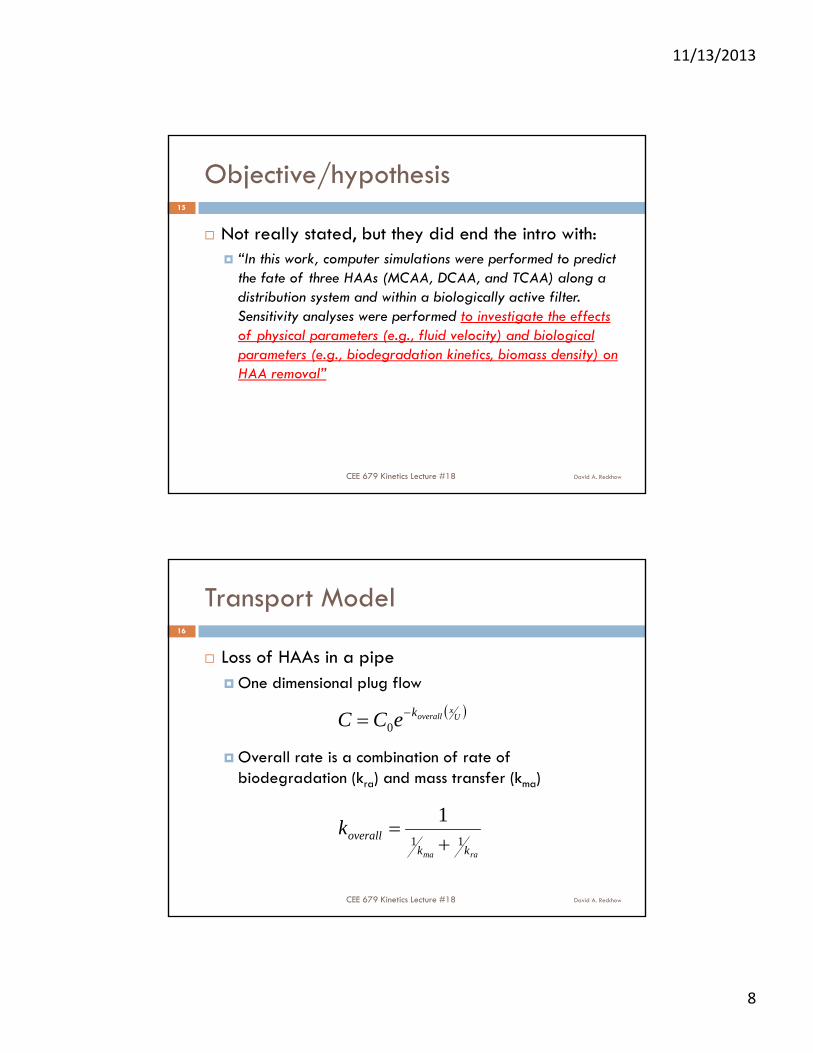
Objective/hypothesis

Not really stated, but they did end the intro with: “In this work, computer simulations were performed to predict

the fate of three HAAs (MCAA, DCAA, and TCAA) along a distribution system and within a biologically active filter. Sensitivity analyses were performed to investigate the effects of physical parameters (e.g., fluid velocity) and biological parameters (e.g., biodegradation kinetics, biomass density) on HAA removal”

David A. Reckhow

15


Transport Model

Loss of HAAs in a pipe One dimensional plug flow

Overall rate is a combination of rate of biodegradation (kra) and mass transfer (kma)

Ux

overallkeCC 0

rama kkoverallk

11

1

David A. Reckhow

16


11/13/2013

9

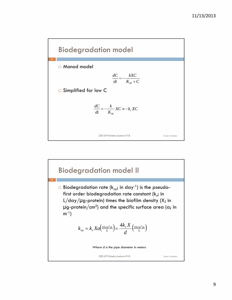
Biodegradation model

Monod model

Simplified for low C

CK

kXC

dt

dC

M

XCkXCK

k

dt

dCr

M

David A. Reckhow

17


Biodegradation model II

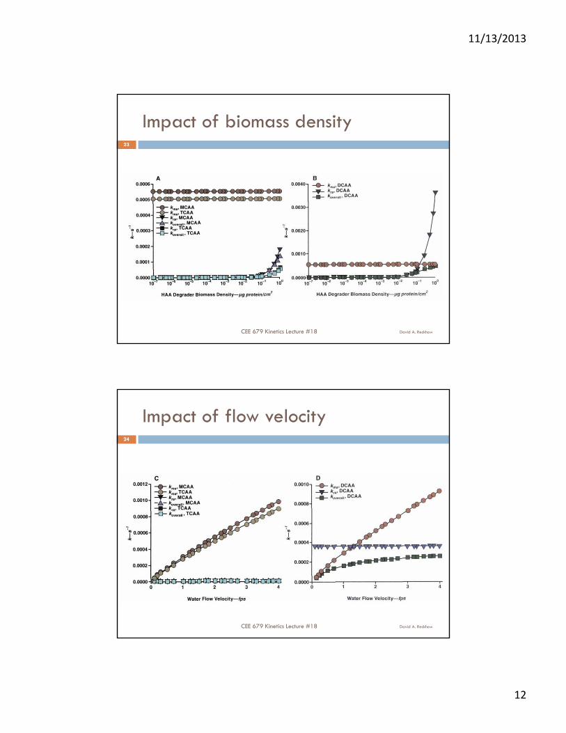
Biodegradation rate (kra; in day-1) is the pseudo-first order biodegradation rate constant (kr; in L/day/µg-protein) times the biofilm density (X; in µg-protein/cm2) and the specific surface area (a; in m-1)

Lmcmr

Lmcm

rra d

XkXakk

22 1010 4

Where d is the pipe diameter in meters

David A. Reckhow

18


11/13/2013

10

David A. Reckhow

19


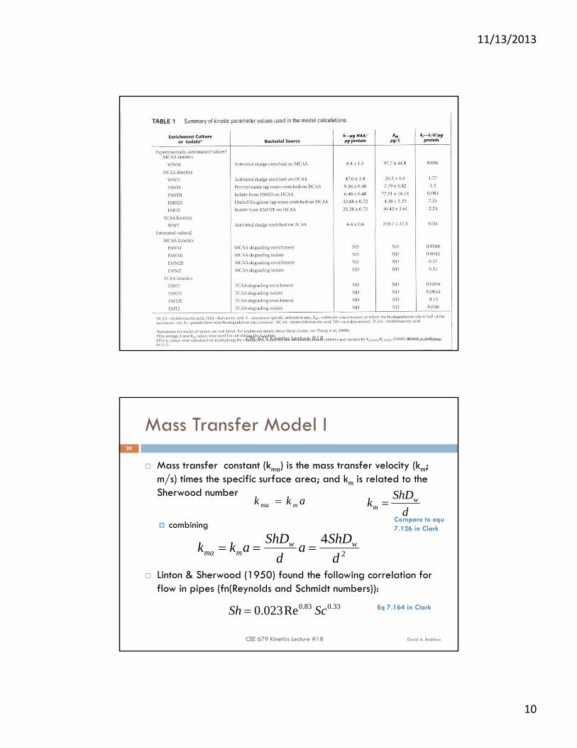
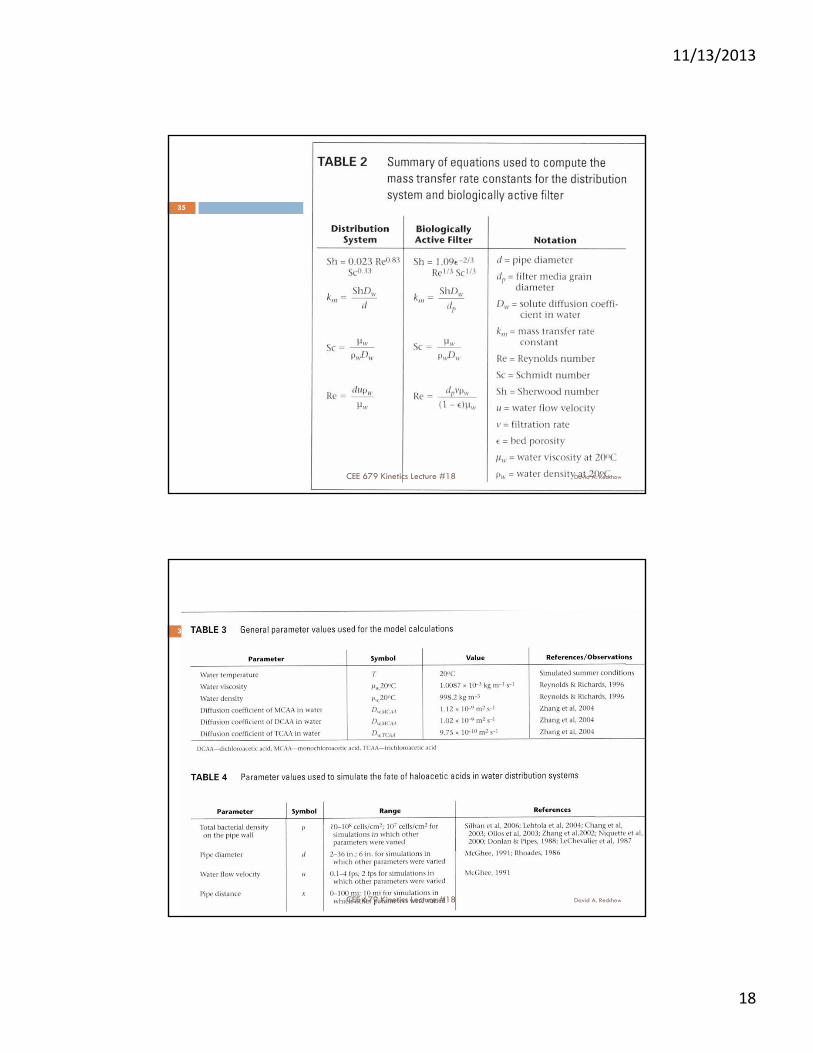
Mass Transfer Model I

Mass transfer constant (kma) is the mass transfer velocity (km; m/s) times the specific surface area; and km is related to the Sherwood number

combining

Linton & Sherwood (1950) found the following correlation for flow in pipes (fn(Reynolds and Schmidt numbers)):

2

4

d

ShDa

d

ShDakk ww

mma

33.083.0Re023.0 ScSh

David A. Reckhow

20


d

ShDk w

m akk mma Compare to equ7.126 in Clark

Eq 7.164 in Clark

11/13/2013

11

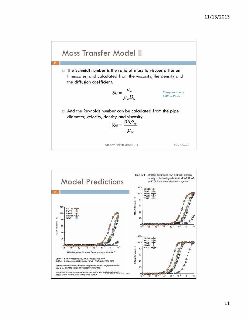
Mass Transfer Model II

The Schmidt number is the ratio of mass to viscous diffusion timescales, and calculated from the viscosity, the density and the diffusion coefficient:

And the Reynolds number can be calculated from the pipe diameter, velocity, density and viscosity:

ww

w

DSc

w

wdu

Re

David A. Reckhow

21


Compare to equ7.82 in Clark

Model Predictions

David A. Reckhow

22


11/13/2013

12

Impact of biomass density

David A. Reckhow

23


Impact of flow velocity


24

11/13/2013

13

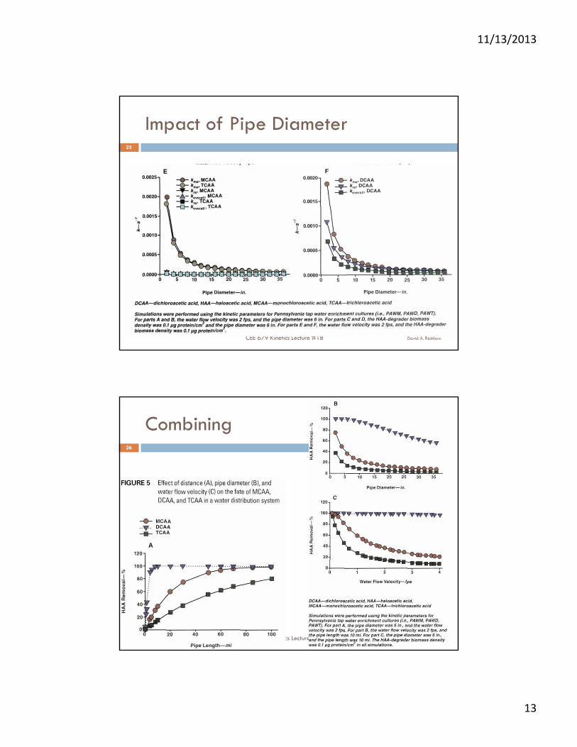
Impact of Pipe Diameter

David A. Reckhow

25


Combining


26

11/13/2013

14

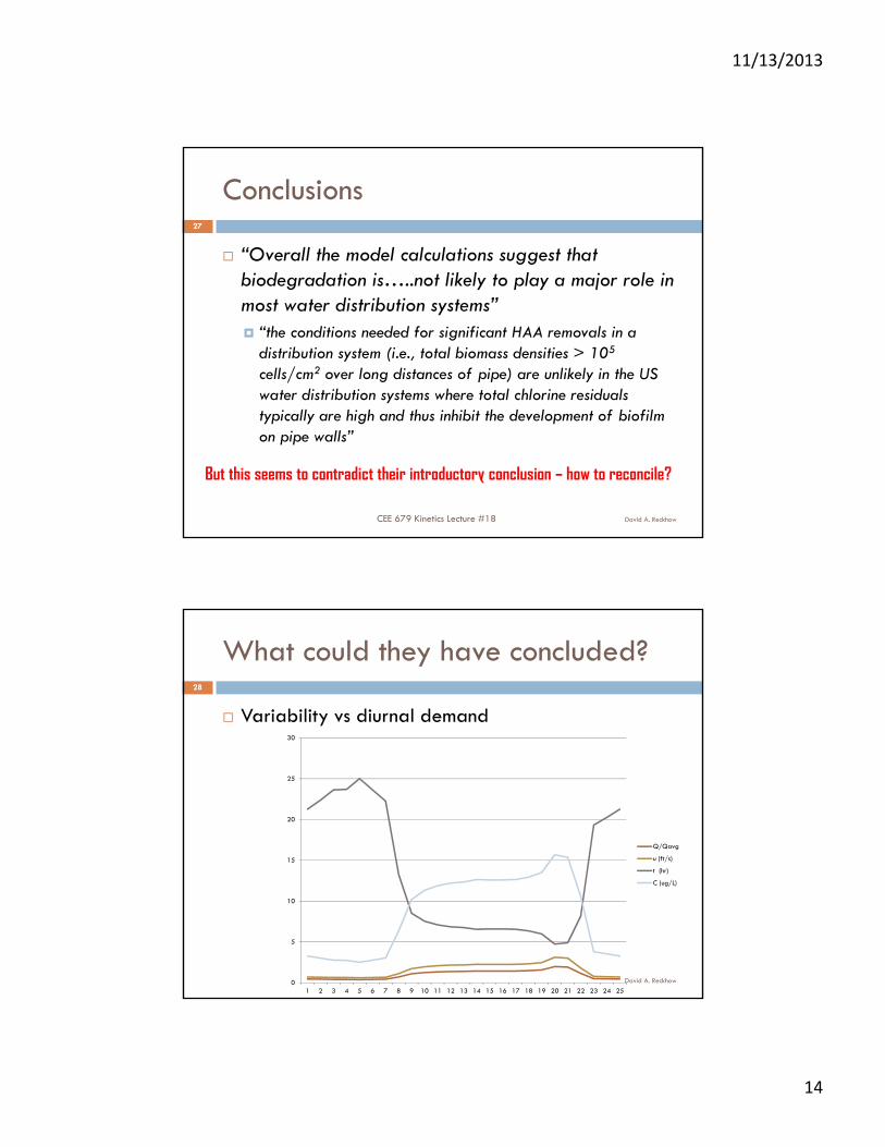
Conclusions

“Overall the model calculations suggest that biodegradation is…..not likely to play a major role in most water distribution systems” “the conditions needed for significant HAA removals in a

distribution system (i.e., total biomass densities > 105

cells/cm2 over long distances of pipe) are unlikely in the US water distribution systems where total chlorine residuals typically are high and thus inhibit the development of biofilmon pipe walls”

But this seems to contradict their introductory conclusion – how to reconcile?

David A. Reckhow

27



What could they have concluded?

Variability vs diurnal demand

0

5

10

15

20

25

30

1 2 3 4 5 6 7 8 9 10 11 12 13 14 15 16 17 18 19 20 21 22 23 24 25

Q/Qavg

u (ft/s)

t (hr)

C (ug/L)

David A. Reckhow

28

11/13/2013

15

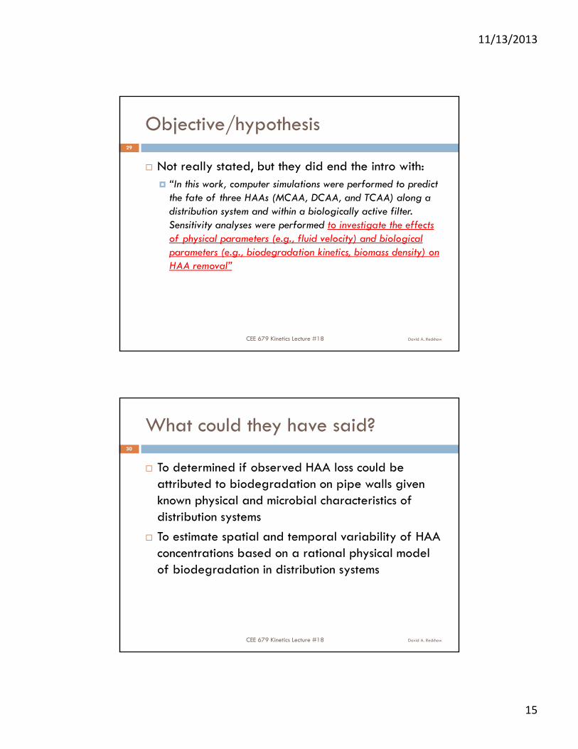
Objective/hypothesis

Not really stated, but they did end the intro with: “In this work, computer simulations were performed to predict

the fate of three HAAs (MCAA, DCAA, and TCAA) along a distribution system and within a biologically active filter. Sensitivity analyses were performed to investigate the effects of physical parameters (e.g., fluid velocity) and biological parameters (e.g., biodegradation kinetics, biomass density) on HAA removal”

David A. Reckhow

29


What could they have said?

To determined if observed HAA loss could be attributed to biodegradation on pipe walls given known physical and microbial characteristics of distribution systems

To estimate spatial and temporal variability of HAA concentrations based on a rational physical model of biodegradation in distribution systems

David A. Reckhow

30


11/13/2013

16

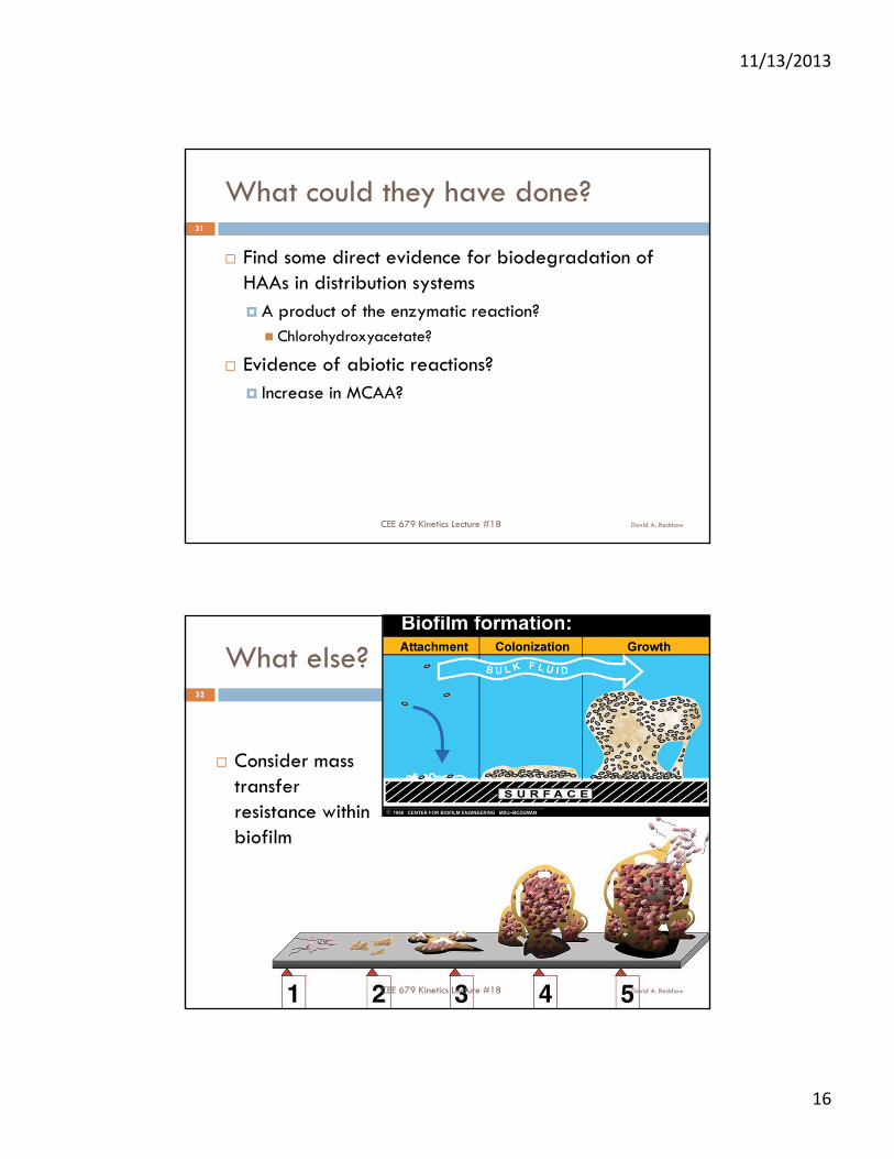
What could they have done?

Find some direct evidence for biodegradation of HAAs in distribution systems A product of the enzymatic reaction? Chlorohydroxyacetate?

Evidence of abiotic reactions? Increase in MCAA?

David A. Reckhow

31


What else?

Consider mass transfer resistance within biofilm

David A. Reckhow

32


11/13/2013

17

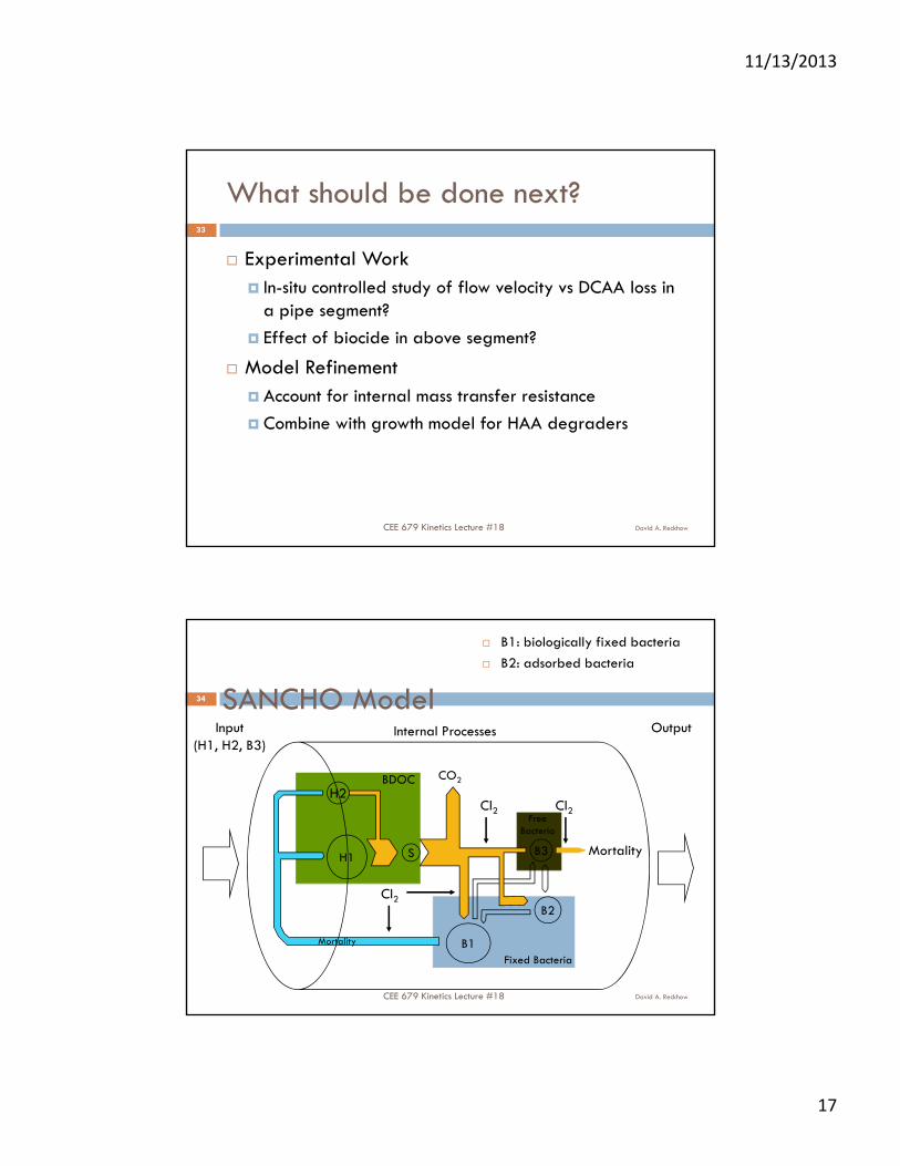
What should be done next?

Experimental Work In-situ controlled study of flow velocity vs DCAA loss in

a pipe segment?

Effect of biocide in above segment?

Model Refinement Account for internal mass transfer resistance

Combine with growth model for HAA degraders

David A. Reckhow

33


SANCHO Model

B1: biologically fixed bacteria

B2: adsorbed bacteria

34

B1

B2

H1

H2

S

CO2

Cl2

MortalityB3

Cl2

Cl2

Mortality

BDOC

Fixed Bacteria

FreeBacteria

Input(H1, H2, B3)

OutputInternal Processes


11/13/2013

18

David A. Reckhow

35


David A. Reckhow

36


11/13/2013

19

David A. Reckhow

37


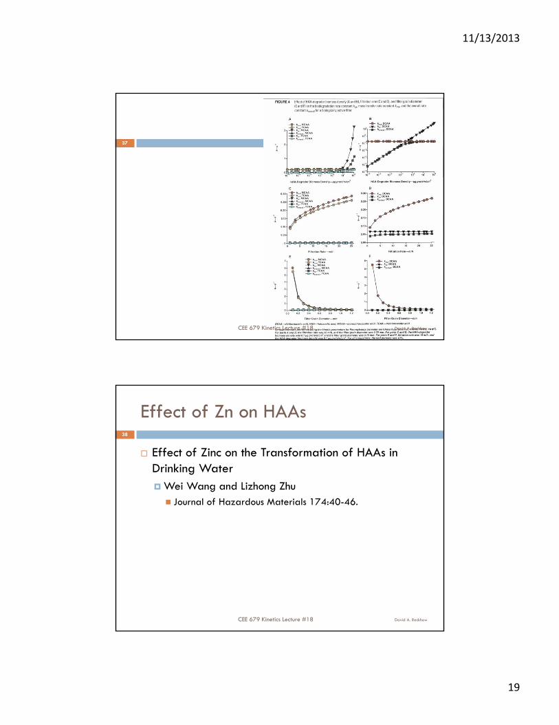
Effect of Zn on HAAs


38

Effect of Zinc on the Transformation of HAAs in Drinking Water Wei Wang and Lizhong Zhu Journal of Hazardous Materials 174:40-46.

11/13/2013

20


39

To next lecture

ENVIRONMENTAL REACTION KINETICS Lecture #18 REACTION KINETICS David A. Reckhow Introduction ... No...

Documents

Transcript of ENVIRONMENTAL REACTION KINETICS Lecture #18 REACTION KINETICS David A. Reckhow Introduction ... No...