Environmental Predictors of Body Mass Index at the Neighborhood Level

Neal SimonsenSchool of Public Health &

Stanley S. Scott Cancer Center

nsimon@lsuhsc.edu

LOUISIANA REMOTE SENSING and GIS WORKSHOP - 2008

Environmental Predictors of Body Mass Index at the Neighborhood Level

Based primarily on:Multilevel Exploration of Obesity Risk for

Cancer PreventionCo-investigators & Collaborators: Richard Scribner, Karen Mason, Joseph Su, Katherine Theall, Cathy Correa, Ed PetersSource of funds: NCI RO3 CA103484

Environmental Predictors of Body Mass Index at the Neighborhood Level

Background:A dramatic increase in obesity over past decades

Environmental changes probably key

Factors that affect the balance of energy intake/expenditure?

Increased energy intakeo Increased portion size, meals away from homeo Increased energy density of foodsDecreased energy expenditure

Neighborhood level factors temporally associated

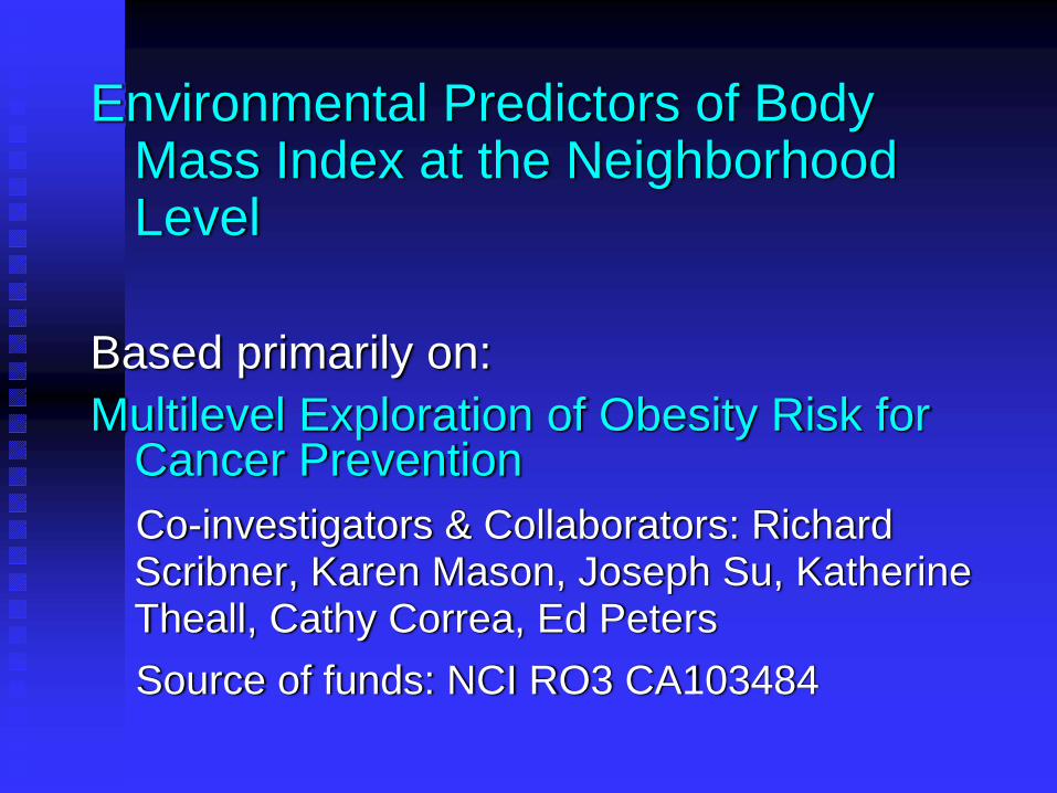
U.S. Trend: Overweight/Obese [NHANES]

-- Prostate Cancer and Prostatic Diseases (2006) 9: 19–24.

Potential relevance for NCI (and cancer)?

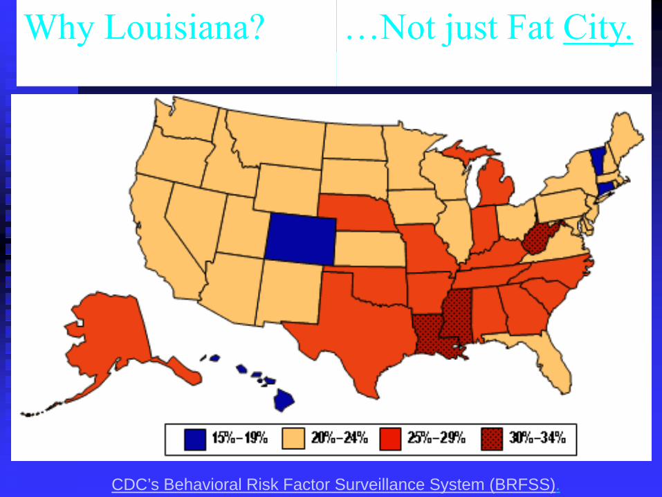
Percent Obese byState [2005 BRFSS]

CDC’s Behavioral Risk Factor Surveillance System (BRFSS).

Why Louisiana? …Not just Fat City.

Individual Level Conceptuality/Study

Physical Activity Overweight Obesity

BMI Weight for

Height

Steps/day Pedometer

Walking trips/wk

Multi Level Conceptual Model

Individual Level

Neighborhood Level

Neighborhood Walkability

Physical Activity Overweight Obesity

BMI Weight for

Height

Steps/day Pedometer

Walking trips/wk

Neighborhood Mix Street Networks

Mean Distance to Closet Store

Mean Number of Routes to Closest

Store

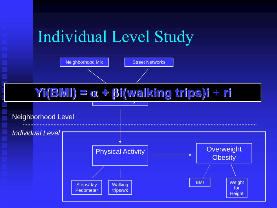
Individual Level Study

Individual Level

Neighborhood Level

Neighborhood Walkability

Physical Activity Overweight Obesity

BMI Weight for

Height

Steps/day Pedometer

Walking trips/wk

Neighborhood Mix Street Networks

Yi(BMI) = α + βi(walking trips)i + ri

Ecologic Study

Individual Level

Neighborhood Level

Neighborhood Walkability

Physical Activity Overweight Obesity

BMI Weight for

Height

Steps/day Pedometer

Walking trips/wk

Neighborhood Mix Street Networks

Obese Neighborhoods

% Obese Mean BMI

Yj(Mean BMI) = α + βj (neighborhood mix)j + uj

Multi Level Study

Individual Level

Neighborhood Level

Neighborhood Walkability

Physical Activity Overweight Obesity

BMI Weight for

Height

Steps/day Pedometer

Walking trips/wk

Neighborhood Mix Street Networks

Yij(Trips/wk) = β0j + rij

β0j (Mean Trips/wk) = γ00 + γ01 (Neighborhood Mix)j + u0j

Yij(Trips/wk) = γ00 + γ01 (Neighborhood Mix)j + u0j + rij

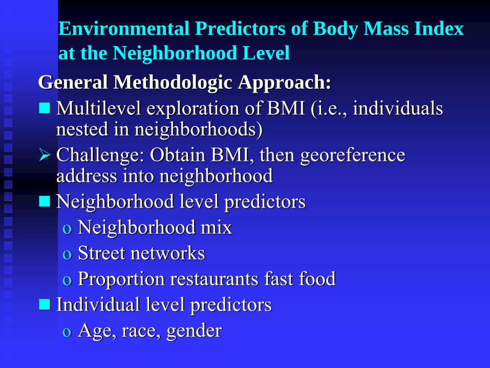
Environmental Predictors of Body Mass Index at the Neighborhood Level

General Methodologic Approach:Multilevel exploration of BMI (i.e., individuals nested in neighborhoods)Challenge: Obtain BMI, then georeference address into neighborhoodNeighborhood level predictors o Neighborhood mix o Street networkso Proportion restaurants fast food

Individual level predictorso Age, race, gender

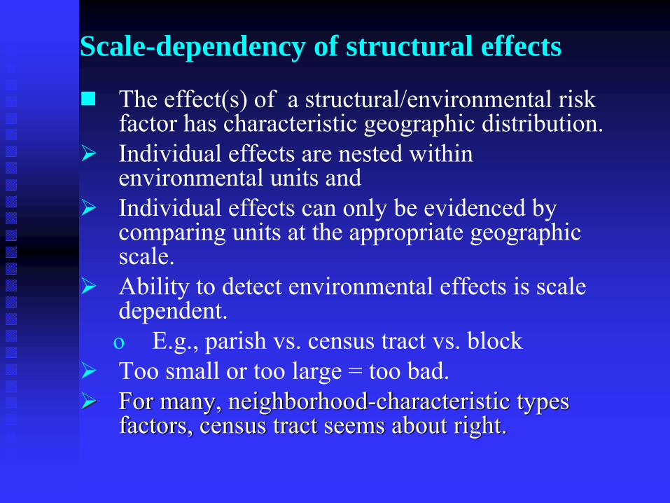
Scale-dependency of structural effects

The effect(s) of a structural/environmental risk factor has characteristic geographic distribution. Individual effects are nested within environmental units andIndividual effects can only be evidenced by comparing units at the appropriate geographic scale.Ability to detect environmental effects is scale dependent. o E.g., parish vs. census tract vs. blockToo small or too large = too bad.For many, neighborhood-characteristic types factors, census tract seems about right.

Drivers Licenses and BMIObtaining individual BMI normally requires interview or visit…LMRICS population-based case control study of lung cancer in communities within the industrial corridor of the MississippiControls as well as cases located through use of driver’s license dataBrainstorm: Can license-reported weight → usable BMI data?

Pearson Coefficient

Spearman Coefficient

Weight .862* .870* BMI .803* .836* * p<0.001

Correlations between Driver’s License-derived and Interview-derived Anthropometric measures for Individuals in the LMRICS Study (Controls, n=442).

DL data → usable BMI

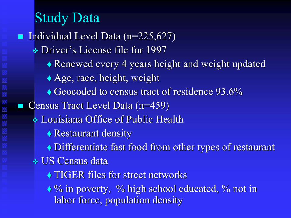
Study DataIndividual Level Data (n=225,627)

Driver’s License file for 1997 Renewed every 4 years height and weight updated Age, race, height, weightGeocoded to census tract of residence 93.6%

Census Tract Level Data (n=459)Louisiana Office of Public Health

Restaurant density Differentiate fast food from other types of restaurant

US Census dataTIGER files for street networks% in poverty, % high school educated, % not in labor force, population density

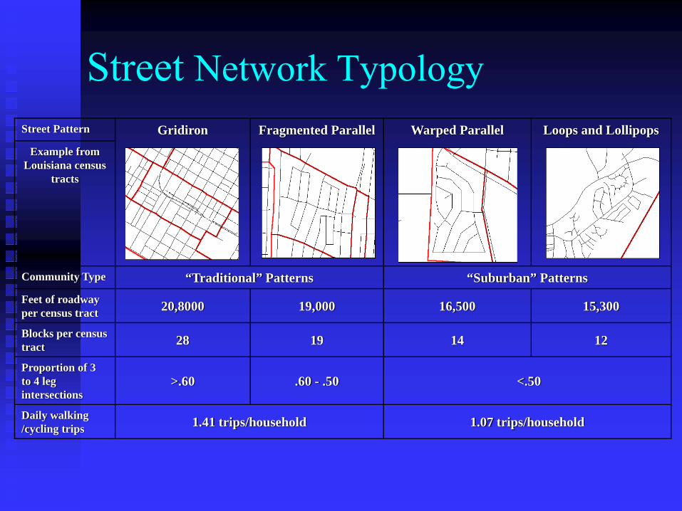
Street Network TypologyStreet Pattern Gridiron Fragmented Parallel Warped Parallel Loops and Lollipops

Example from Louisiana census

tracts

Community Type “Traditional” Patterns “Suburban” PatternsFeet of roadway per census tract 20,8000 19,000 16,500 15,300

Blocks per census tract 28 19 14 12

Proportion of 3 to 4 leg intersections

>.60 .60 - .50 <.50

Daily walking /cycling trips 1.41 trips/household 1.07 trips/household

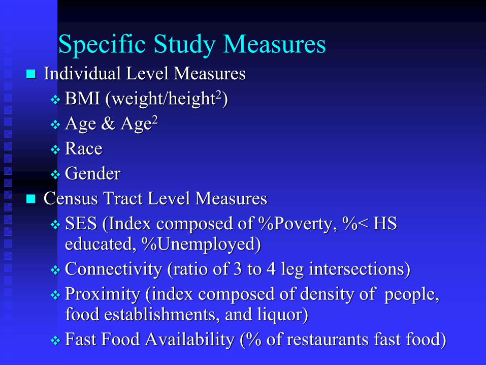
Specific Study MeasuresIndividual Level Measures

BMI (weight/height2)Age & Age2

RaceGender

Census Tract Level MeasuresSES (Index composed of %Poverty, %< HS educated, %Unemployed)Connectivity (ratio of 3 to 4 leg intersections)Proximity (index composed of density of people, food establishments, and liquor)Fast Food Availability (% of restaurants fast food)

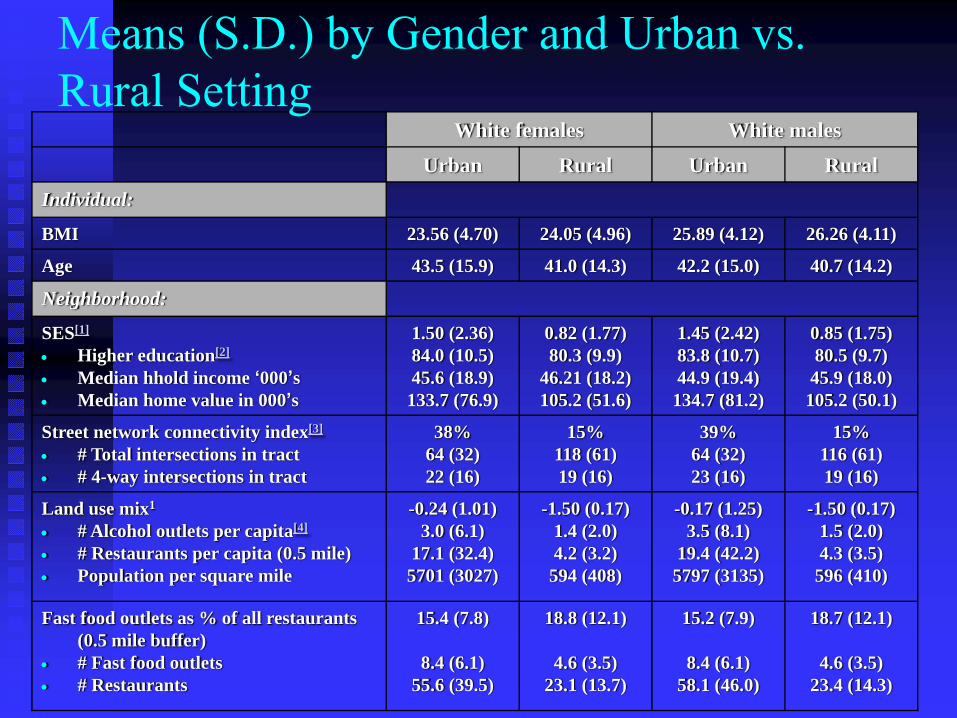
White females White males

Urban Rural Urban RuralIndividual:

BMI 23.56 (4.70) 24.05 (4.96) 25.89 (4.12) 26.26 (4.11)

Age 43.5 (15.9) 41.0 (14.3) 42.2 (15.0) 40.7 (14.2)

Neighborhood:

SES[1]

• Higher education[2]

• Median hhold income ‘000’s• Median home value in 000’s

1.50 (2.36)84.0 (10.5)45.6 (18.9)133.7 (76.9)

0.82 (1.77)80.3 (9.9)

46.21 (18.2)105.2 (51.6)

1.45 (2.42)83.8 (10.7)44.9 (19.4)134.7 (81.2)

0.85 (1.75)80.5 (9.7)45.9 (18.0)105.2 (50.1)

Street network connectivity index[3]

• # Total intersections in tract• # 4-way intersections in tract

38% 64 (32)22 (16)

15%118 (61)19 (16)

39%64 (32)23 (16)

15%116 (61)19 (16)

Land use mix1

• # Alcohol outlets per capita[4]

• # Restaurants per capita (0.5 mile)• Population per square mile

-0.24 (1.01)3.0 (6.1)

17.1 (32.4)5701 (3027)

-1.50 (0.17)1.4 (2.0)4.2 (3.2)

594 (408)

-0.17 (1.25)3.5 (8.1)

19.4 (42.2)5797 (3135)

-1.50 (0.17)1.5 (2.0)4.3 (3.5)

596 (410)

Fast food outlets as % of all restaurants (0.5 mile buffer)

• # Fast food outlets • # Restaurants

15.4 (7.8)

8.4 (6.1)55.6 (39.5)

18.8 (12.1)

4.6 (3.5)23.1 (13.7)

15.2 (7.9)

8.4 (6.1)58.1 (46.0)

18.7 (12.1)

4.6 (3.5)23.4 (14.3)

Means (S.D.) by Gender and Urban vs. Rural Setting

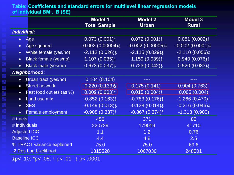
Table: Coefficients and standard errors for multilevel linear regression models of individual BMI. Β (SE) Model 1 Model 2 Model 3 Total Sample Urban Rural Individual:

• Age 0.073 (0.001)‡ 0.072 (0.001)‡ 0.081 (0.002)‡ • Age squared -0.002 (0.00004)‡ -0.002 (0.00005)‡ -0.002 (0.0001)‡ • White female (yes/no) -2.112 (0.026)‡ -2.115 (0.029)‡ -2.110 (0.056)‡ • Black female (yes/no) 1.107 (0.035)‡ 1.159 (0.039)‡ 0.940 (0.076)‡ • Black male (yes/no) 0.673 (0.037)‡ 0.723 (0.042)‡ 0.520 (0.083)‡

Neighborhood: • Urban tract (yes/no) 0.104 (0.104) ---- ---- • Street network -0.220 (0.133)§ -0.175 (0.141) -0.904 (0.763) • Fast food outlets (as %) 0.009 (0.003)† 0.015 (0.004)† 0.005 (0.004) • Land use mix -0.852 (0.163)‡ -0.783 (0.176)‡ -1.266 (0.470)† • SES -0.149 (0.013)‡ -0.138 (0.014)‡ -0.216 (0.046)‡ • Female employment -0.908 (0.337)† -0.867 (0.374)* -1.313 (0.900)

# tracts 456 371 85 # individuals 220729 179019 41710 Adjusted ICC 1.1 1.2 0.76 Baseline ICC 4.4 4.8 2.5 % TRACT variance explained 75.0 75.0 69.6 -2 Res Log Likelihood 1315528 1067030 248501 §p< .10: *p< .05: † p< .01: ‡ p< .0001

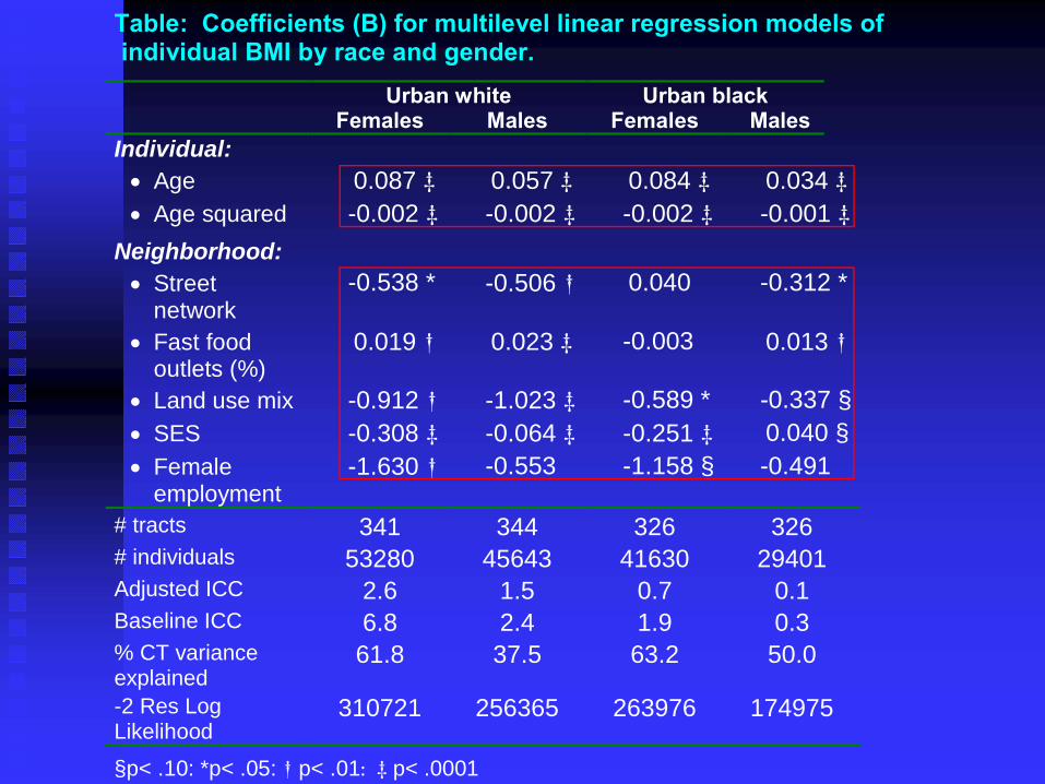
Table: Coefficients (B) for multilevel linear regression models of individual BMI by race and gender. Urban white Urban black Females Males Females Males Individual: • Age 0.087 ‡ 0.057 ‡ 0.084 ‡ 0.034 ‡• Age squared -0.002 ‡ -0.002 ‡ -0.002 ‡ -0.001 ‡

Neighborhood: • Street

network -0.538 * -0.506 † 0.040 -0.312 *

• Fast food outlets (%)

0.019 † 0.023 ‡ -0.003 0.013 †

• Land use mix -0.912 † -1.023 ‡ -0.589 * -0.337 §• SES -0.308 ‡ -0.064 ‡ -0.251 ‡ 0.040 §• Female

employment -1.630 † -0.553 -1.158 § -0.491

# tracts 341 344 326 326 # individuals 53280 45643 41630 29401 Adjusted ICC 2.6 1.5 0.7 0.1 Baseline ICC 6.8 2.4 1.9 0.3 % CT variance explained

61.8 37.5 63.2 50.0

-2 Res Log Likelihood

310721 256365 263976 174975

§p< .10: *p< .05: † p< .01: ‡ p< .0001

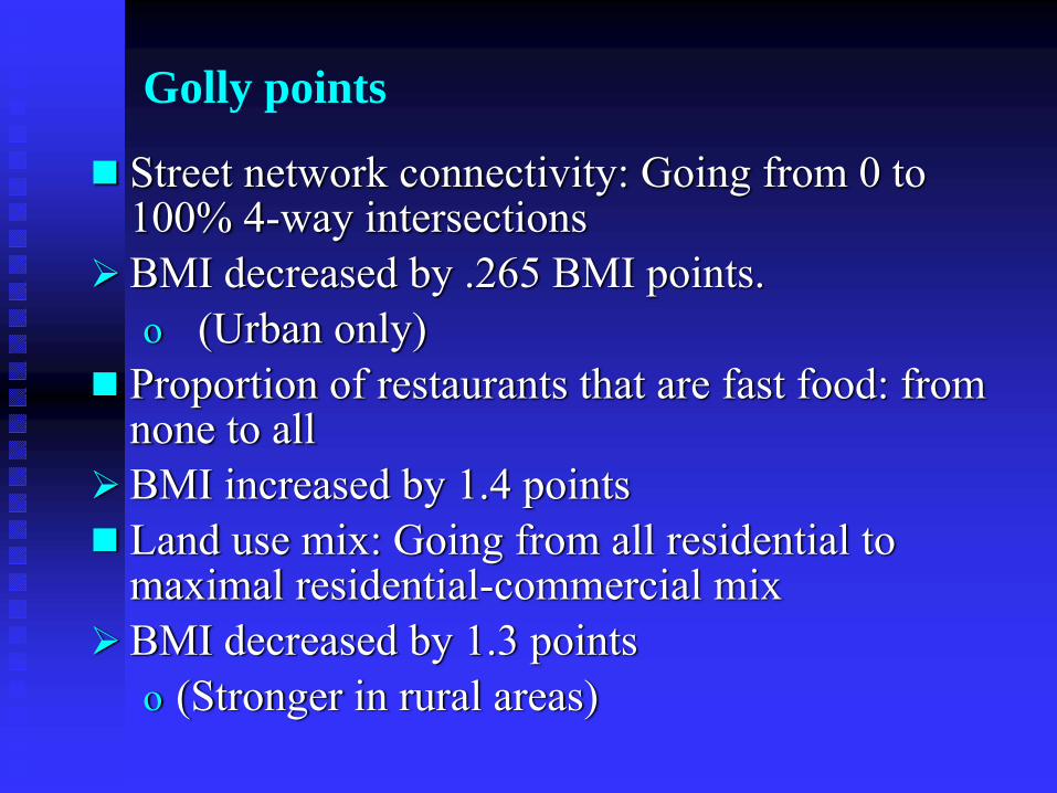
Golly points

Street network connectivity: Going from 0 to 100% 4-way intersections BMI decreased by .265 BMI points.o (Urban only)

Proportion of restaurants that are fast food: from none to allBMI increased by 1.4 pointsLand use mix: Going from all residential to maximal residential-commercial mixBMI decreased by 1.3 pointso (Stronger in rural areas)

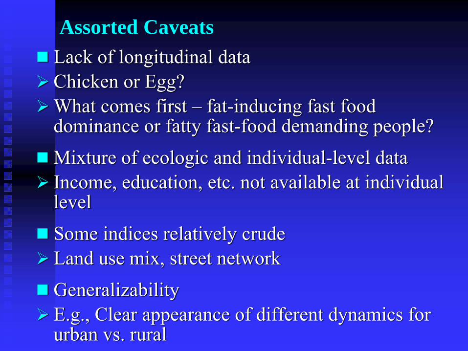
Assorted CaveatsLack of longitudinal dataChicken or Egg?What comes first – fat-inducing fast food dominance or fatty fast-food demanding people? Mixture of ecologic and individual-level dataIncome, education, etc. not available at individual levelSome indices relatively crudeLand use mix, street networkGeneralizabilityE.g., Clear appearance of different dynamics for urban vs. rural

Fini!

What are Community Influences on Health Behavior and Why Do We Care?

WhatCommunity environment affects health behaviorType of influence

direct influenceindirect influenceInteractive influence

Other names contextual effects, group level effects, exogenous effects, cross level effects, structural effects

WhyPreventive potential

primary prevention workslow costlimited success of individual level interventionspopular

Environmental justiceviolation of human rightsresponsible for health disparities?

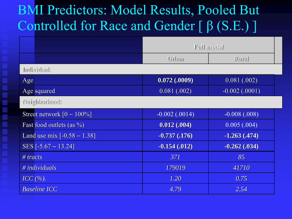
Full model

Urban Rural

Individual:

Age 0.072 (.0009) 0.081 (.002)

Age squared 0.081 (.002) -0.002 (.0001)

Neighborhood:

Street network [0 – 100%] -0.002 (.0014) -0.008 (.008)

Fast food outlets (as %) 0.012 (.004) 0.005 (.004)

Land use mix [-0.58 – 1.38] -0.737 (.176) -1.263 (.474)

SES [-5.67 – 13.24] -0.154 (.012) -0.262 (.034)

# tracts 371 85

# individuals 179019 41710

ICC (%). 1.20 0.75

Baseline ICC 4.79 2.54

BMI Predictors: Model Results, Pooled But Controlled for Race and Gender [ β (S.E.) ]