ENVIRONMENTAL EFFECTS ON PAVEMENTS
182
ENVIRONMENTAL EFFECTS ON PAVEMENTS Damage Analysis Shang J. Liu Robert L. Lytton Texas Transportation Institute Texas A&M University Systems August 1983
Transcript of ENVIRONMENTAL EFFECTS ON PAVEMENTS

ENVIRONMENTAL EFFECTS ON PAVEMENTS
Damage Analysis
Shang J. Liu
Robert L. Lytton
Texas Transportation Institute
Texas A&M University Systems
August 1983

This electronic document was created from an
original hard-copy.
Due to its age, it may contain faded, cut-off or
missing text or low-quality images.

ACKNOWLEDGEMENTS
This research report has been funded by the Federal
Highway Administration and a subcontract from the University
of Illinois at Urbana. The authors gratefully acknowledge
the support received from these sources.
DISCLAIMER
The contents of this report reflect the views of the
authors who are responsible for the facts and the accuracy
of the data presented within. The contents do not
necessarily reflect the official views of policies of the
Federal Highway Administration. This report does not
constitute a standard, a specification or regulation.
ll

TABLE OF CONTENTS
Page
CHAPTER 1 INTRODUCTION • ••.•••••••••••••••••••••••••••••.•• 1
CHAPTER 2 MODELS OF RAINFALL DISTRIBUTION AND FREQUENCY ANALYSIS........................................ 11
2.1 Probability Model of Quantity of Rainfall....... 11
2.2 Models of Intensity and Duration of Rainfall.... 13
2.3 Frequency Models of Rainfall - Markov Chain Method and Dry and Wet Day Probabilities......... 15-
CHAPTER 3 INFILTRATION OF WATER INTO A PAVEMENT THROUGH CRACKS AND JOINTS •..•....••..•••..•..•••.•.••••.
3.1 Laboratory Studies ..•••••..••••...•.•••••.•••..•
3.2 Field Observations ............................. .
3.3 Low Permeability Base Courses •••.•••.•••••••••••
3.3.1 Water Entry into Low Permeability Bases .••.•
3.3.2 Water Evaporation from the Base Course .•••.•
CHAPTER 4 DRAINAGE OF WATER OUT OF BASE COURSES ..•••..•...
4.1 Casagrande's and Shannon's Method •••••••••••••••
4.2 Parabolic Phreatic Surface Method with an Impermeable Subgrade .••••..•.•.•.•••••.•.•••••••
4.3 Analysis of Subgrade Drainage ..........•..•.•...
4.4 Drainage with a Parabolic Phreatic Surface and a Permeable Subgrade ••..•..........•.•......•...
4.5 Application to Pavement Drainage Design •...•••••
4.6 Estimation of Drainability of the Base Course and Evaluation of Drainage Design ..••••••.••••••
CHAPTER 5 EFFECT OF WATER SATURATION ON LOAD-CARRYING CAPACITY OF BASE COURSE AND SUBGRADE ..•••••.••..
5.1 Effect of Saturation on Base Course Properties ..
5.2 Effect of Saturation on Subgrade Properties •.•••
iii
21
21
23
24
25
27
29
29
36
38
45
46
52
57
57
61

CHAPTER 6 SYNTHESIS OF THE METHODS OF RAINFALL, INFILTRATION, DRAINAGE, AND LOAD-CARRYING CAPACITY OF A PAVEMENT •••••••••••••.••••.••••••••••••••••
6.1 Conceptual Flow Chart for Rainfall, Infiltra-tion and Drainage Analysis ..................... .
6.2 Synthesis of the Methods of Rainfall Model, ;nfiltration and Drainage Analysis ....•.........
6.3 Data Required for Analysis and Sample Results .••
6.4 An Example of Systematic Analysis of Rainfall Infiltration, Drainage, and Load-Carrying Capacity of Pavements •...•..•....•..............
CHAPTER 7 CONCLUSIONS AND RECOMMENDATIONS .••....•.•.•••.•.
REFERENCES . •.•.••••.••••••••••••••• ·• •.••••••••••••••••••••••
APPEND ICES •• •••••.••••••••••••••••••••••••••••••••••••••••••
A Rainfall Amount Distribution, Rainfall Duration
B
c
and Markov Chain Model ....•....•..•..••.•..•..•.
Parabolic Phreatic Surface Drain Models for Base Courses with Impermeable Subgrade .•.••..••.
Parabolic Phreatic Surface Drain Models for Base Courses with Subgrade Drainage .••.•.....•.......
D Entry and Evaporation of Water in a Low
Page
64
65
68
75
81
84
85
88
88
96
105
Permeability Base Course........................ 115
E Flow Chart, Computer Programming and User's Guide........................................... 124
iv

LIST OF TABLES
TABLE Page
1. Katz's Model for Computing the Wet Probabilities Associated with Markov Chain Model.................. 19
2. Drainability of Water in the Base Courses from a Saturated Sample ................................... . 54
3. Calculated Elastic Moduli for Materials in the TTI Pavement Test Facility •••••••••••••••••••••••••••••• 60
4. Regression Coefficients for the Effect of Degree of Saturation on Elastic Moduli of Subgrade Soils...... 62
5. TTI Drainage Model for an Analysis of a Houston Pavement •••••••••••••••••••••••••••••••••••••••••••• 73
6. TTI Drainage Model for Evaluation of a Drainage Design of a Houston Pavement........................ 74
7. Markov Chain Model and for Dry Probabilities
Katz's Recurrence Equations versus a Drainage Curve of a
Houston Pavement ••••••••••••.•••••••••••••••••••••••
8. Stochastic Models for a System Analysis of Rainfall Infiltration and Drainage Analysis of a Houston Pavement •..•••••••••••••••.•.•...•••••.•.•••••••••••
9. Evaluation of a Rainfall Effect on Pavement Performance of a Houston Pavement •..••.•••••.••.•••.
v
76
77
79

LIST OF FIGURES
FIGURE
1. Comparison of Normal and Gumble Distributions .••••.•
2. Rainfall Infiltration and Evaporation Through Cracks and Joints in a Low Permeability Base ••.••••.
3. Cross Section of a Pavement ••.•..•.••.•....••••.••..
4. Casagrande-Shannon Model for Base Course Drainage .••
5. Variation of Drainage Area with Slope Factor and Time Factor ........................................ .
6. TTI Model for Base Course Drainage with an Impermeable Subgrade ••••••••••••••••.•••••••••......
7. TTI Drainage Chart with an Impermeable Subgrade ••••.
8. Comparison of Results for an Impermeable Subgrade ••.
9. Comparison of Results for an Impermeable Subgrade •.•
10. Comparison of Results for an Impermeable Subgrade •.•
ll. Permeable Subgrade with Casagrande-Shannon Drainage Model ..................................... .
12. Definition Sketch for Subgrade Drainage Model .....••
13. Subgrade Drainage Model with Parabolic Phreatic Surfaces ........................................... .
14. Results of TTI Model with Permeable Subgrade ...•••••
15. Results of TTI Model with Permeable Subgrade •....•..
16. Drainage Curves for TTI Model with Permeable Subgrades •.•.......•.•.•••........•..•.•.........•..
17. Effect of Amount and Type of Fines on the Permeab i 1 i ty . ...................................... .
18. Drainage Criteria for Granular Layers •••••••.•...•••
19. Effect of the Degree of Saturation on the Repeated-Load Deformation Properties of the AASHO Granular Mater i a l s ................................. .
20. Flow Chart for Conceptual Model of Rainfall Infiltration and Drainage Analysis of Pavements ..••.
vi
Page
16
26
30
31
33
37
39
40
41
42
43
44
47
48
49
51
53
56
59
66

21. Synthesis of Models Used in Rainfall Infiltration and
Systematic Analysis of Drainage Analysis of a
Pavement............................................ 67
22. Effects of Rainfall Amount and Subgrade Drainage on Load-Carrying Capacity of Pavements................. 83
23. Definition Sketch of Katz Model..................... 94
24. Stages of Parabolic Phreatic Surface in a Horizontal Base................................................ 97
25. Stages of Parabolic Phreatic Surface in a Sloping Base ..................................... -........... 101
26. Water Penetration into a Subgrade without Lateral Drainage............................................ 106
27. Water Penetration into a Subgrade with Lateral Drainage............................................ 107
28. Stages of Parabolic Phreatic Surface with Both Lateral and Subgrade Drainage for a Sloping Base.... 112
29. The Elliptical Shape of Water Penetration and the Evaporation in a Low Permeability Base Course....... 116
30. Relationship between Suction and Moisture Content in Soil................................................ 123
vii

CHAPTER 1 INTRODUCTION
Pavement engineers and road builders have been aware
for a long time that excess water remaining in base courses
and subgrades will accelerate the deterioration and
destruction of pavements. As the water content of base
courses and subgrades increases, there is a significant
reduction in load bearing capacity and modulus and an
acceleration of unsatisfactory pavement performance, as
manifested in premature rutting, cracking, faulting,
pumping, increasing roughness, disintegration of stabilized
materials, and a relatively rapid decrease in the level of
serviceability. In estimating the long-term performance of
pavements and in designing pavements to endure the effects
of the local climate, it is essential to be able to estimate
the effect of rainfall on the modulus of the base course and
subgrade. This paper describes a comprehensive means of
making such estimates and gives the results of example
calculations.
This subject of base
considerable attention over
course drainage
the last three
has received
decades. In
1951, Casagrande and Shannon <l> developed models for
drainage
airfields
analysis
in the
and made
United
field observations on several
States to determine the
environmental conditions under which base courses may become
saturated. Most of the observations were limited to two
1

principal causes for the saturation of base courses: frost
action and infiltration through the surface course. At six
airfields, in Maine, Wisconsin, Michigan, North Dakota, and
South Dakota, detailed observations were made, by Casagrande
and Shannon (!) , of groundwater levels in
the base course beneath both concrete
the subgrade in
and bituminous
pavements.
pipes was
The discharge through the base-course drainage
also monitored at those fields. Based on their
observations, they concluded that during the thawing period,
ice segregation in a subgrade may be the cause of saturation
of an overlying, free-draining base. It was also concluded
that infiltration of surface water through pavement cracks,
or joints, may cause saturation of a free-draining base
overlying a relatively impervious subgrade. Other causes
for the saturation of bases may be inundation of the
pavement in an area that might be subject to flooding during
certain times of the year, or where the natural water table
may rise above the bottom of the base course.
One cause of excess moisture content in the pavement,
mainly
through
amount
due to climatic conditions, is rainfall infiltration
cracks and joints. Methods for estimating the
of rainfall and subsequent water infiltration through
cracks and joints have been developed by Cedergren (~) and
Markow (l), both of whom mention the lack of adequate
field observation data on this subject. Markow simulated
pavement performance under various moisture conditions by
2

incorporating the amount of unsealed cracking 1n the
pavement surface, the seasonal rainfall, and the quality of
subsurface drainage into the modeling. He also pointed out
that in pavements subjected to rainfall infiltration, three
periods associated with wet weather can be distinguished:
l. the time during which rain is falling, in which
the pavement sublayers may or may not be
saturated;
2. the time during which the sublayers are saturated
or sufficiently wet to affect material properties
and structural behavior; and
3. the time during which any residual water not
sufficient to affect pavement behavior is drained
off.
Nevertheless, in Markow's model, in order to simplify
the derivation of the models, only the second period above
was considered, i.e., the period during which the pavement
is significantly wet or saturated to effect material
properties and structural behavior. The model is used in
the EAROMAR system, which is a simulation model of freeway
performance used by the Federal Highway Administration in
conducting economic analyses of various strategies of
roadway and pavement reconstruction, rehabilitation, and
maintenance. As a conservative estimate, during the time
required to drain 80% of the water from a saturated
sublayer, the sublayer modulus was considered to be reduced
3

in value by 50%.
As used to estimate the change of the elastic modulus
of base course materials due to water entering the base
course through' cracks and joints in the pavements, the
EAROMAR equation is
where
twet = (yseason1iavg> [1-exp(-gc)]tdrain
c = (1/5280){[(L +A )/Wl ]+[(SH X w t)/ c c ane we
F red
2WlaneNlane]+(J x Wwet)}
= (tseason-O.Stwet)/tseason
twet = duration of pavement wetness in
( 1-1)
( 1-2)
(1-3)
days
during which structural response is
assumed to be affected;
Yseason = seasonal rainfall in inches input by the
user;
i = daily rainfall intensity, assumed to equal avg
0.5 in {12.7 mm);
c = fraction of pavement area having cracks or
td . ra1n =
open (unsealed) joints;
time in days to drain
pavement sublayers;
the saturated
Lc' Ac = quantities of damage components per lane
SH, J mile computed by pavement simulation
models within EAROMAR; L ' c SH, and J
are the linear feet per lane mile of lon-
gitudinal cracks, lane-shoulder joints,
4

and transverse joints; A is the area c
of alligator cracking in square feet per
lane mile;
W N - width of lane in feet and number of lanes lane' lane -
in roadway, respectively, as input by
user;
W = width of subsurface zone wetted by open wet
joint, assumed to be 6ft (1.8 m);
Fred = reduction factor applied to moduli of
granular pavement layers and to California
bearing ratio (CBR) and moduli of
subgrade;
t = length of season in days determined from season
season information input by user; and
td · is evaluated from ra1n Casagrande-Shannon's drainage
model (l) to be approximately
where
td . = 2.5nL 2 exp(-2S')/KH raln
n = effective porosity of
L = the width of the base
( 1-4)
the base course,
course,
K = the permeability of the base course,
H = the thickness of the base course, assumed
to be l foot, and
s I = an approximate slope factor, assuming a
cross slope of l/2 inch per foot (0.015
ft/ft).
5

Equation 1-3 applies a time-average correction to the
pavement materials properties. Multiplication by 0.5 in
Equation 1-3 reflects the assumed loss in ~aterial strength
under wet condition.
Equation 1-3 is composed of three factors: ( 1) the
number of days in a season on which rainfall occurs,
yseason/iavg; ( 2) the proportion of rainfall flowing
into the base courses, l-exp{-9c); and (3) the period of
time over which the structural response is reduced to its
50% level These three factors are multiplied
together in that equation and give the total amount of time
(t t) we when the base courses are at least 20% saturated.
Briefly, the time, in days, that a base course is in such a
wet situation is equal to the number of wet days in a season
multiplied by the time required to drain 80% of water, where
the proportion of infiltration is taken into consideration.
The following assumptions are implied.
1. The amount of water inflow into the base courses
is a negative exponential function of rainfall
quantity. This equation is derived from the data
provided by Cedergren (~).
2. The length of the wet period, t wet' is
linearly related to the time required to drain 80%
of the water from the sublayer.
3. The drainage analysis is approximately based on
Casagrande's and Shannon's model (See
Chapter 4).
6

4. Every rainy day has the same effect on a base
course.
5. Dry days are subsequent to wet days which are
equally spaced in time.
6. The degree of 80% drainage is a critical point for
the elastic moduli of the base courses. Before
80% of drainage is completed, the moduli are
reduced to 50%. After 80% of the water has
drained out of the base course, there is no effect
on the elasticity of the base course.
Nevertheless, certain modifications to Markow's model
should be made for a more realistic and more theoretically
correct approach, especially when Assumptions
considered.
3 to 6 are
For lateral free drainage, in the Casagrande-Shannon
model of base-course drainage (l), the analysis which has
been commonly applied, a linear free water surface is
assumed. This assumption is not consistent with the
theoretical approach derived by Polubarinova-Kochina (!),
which suggests that a parabolic phreatic surface would yield
more realistic results for drainage calculations. Also a
permeable subgrade, which in fact exists in the pavement
structure is not taken into account by the Casagrande
Shannon model.
So far as the rainfall period and probability are
concerned, Markow's model does not consider the distribution
7

of rainfall amount and does not consider wet and dry day
probabilities adequately, i.e. , not every rainy day would
saturate the base course and dry days following each rainy
day do not divide the weather sequence realistically. In
addition, in evaluating the deterioration of pavements, it
is more realistic to allow the elastic moduli of the base
course and subgrade to vary continuously with water content,
than to assume simply that up to 80% drainage the base
course modulus is half of its dry value, which is done in
Markow's model.
In this report, a stochastic model is used for a
systematic analysis of rainfall infiltration, drainage,and
estimation of the material properties of base course and
subgrade. The report describes a model consisting of five
main parts: (1) estimation of the amount of rainfall that
falls each day on a pavement; (2) the infiltration of water
through the cracks and joints in the pavement; (3)
computation of the simultaneous drainage of water into the
subgrade and into the lateral drains; (4) dry and wet
probabilities of the weather and pavement sublayers; and (5)
the effect of changing water contents on the moduli of base
courses and subgrades. Ground water sources and the side
infiltration from the pavement shoulders are not considered
in this report.
A gamma distribution is
probability density function
8
employed for describing the
for the quantity of rain that

falls and a Markov chain model is applied for estimating the
probabilities of wet and dry days.
Infiltration of water into the pavement cracks and
joints uses either Ridgeway's <!!> rate of infiltration of
water through cracks and joints, which was determined in a
field experiment, or the regression equations of Dempsey and
Robnett (~) which were developed from field measurements,
in estimating the amount of free water entering the pavement
base course.
A new method has been developed for computing the
drainage of the pavement base and subgrade. Models
employing a parabolic phreatic surface and allowing drainage
through a permeable subgrade are developed, which generally
give better agreement with field data from observations on
full scale pavements than the classical model described by
Casagrande and Shannon. That model assumes a straight line
phreatic surface and an impermeable subgrade.
A recurrence relation for computing probabilities
associated with the Markov chain model for dry and wet days,
incorporated with the gamma distribution, and the analysis
of infiltration of water into the pavement and subsequent
drainage is applied to estimate the dry and wet
probabilities of the base courses.
The systematic prediction of the degree of free water
saturation in the base courses each day is performed by
combining into the analysis of the distribution of rainfall
9
amount, the probabilities of wet and dry days, infiltration
of water into the pavement, the drainage time of the base
courses, and dry and wet probabilities of the weather and
pavement sublayers.
The effect of saturation on the resilient modulus of
the base course and the subgrade are calculated using
relations presented by Haynes and Yoder (~),
and Robnett (1!,12>, and these may be
and Thompson
used in the
prediction of critical stresses and strains in a pavement to
determine the amount of traffic it can be expected to carry
throughout its useful life.
10

CHAPTER 2 MODELS OF RAINFALL DISTRIBUTION AND
FREQUENCY ANALYSIS
In order to estimate the quantity of rainfall that
falls on a specific pavement and eventually enters the
cracks and joints of that pavement, it is necessary to
establish three items of information concerning the local
rainfall patterns.
1. The quantity of rain that falls
rainfall. The total quantity in
varies from one rainfall to the
in a given
each rainfall
next but
historical records show that the quantity follows
a probability density function.
2. The intensity and duration of each rainfall.
3. The random occurrence of sequences of wet and dry
days.
The methods that are used in estimating these quantities are
described in the following subsections.
2.1 PROBABILITY MODEL OF QUANTITY OF RAINFALL
Applications of new techniques such as stochastic
processes, time series analysis, probabilistic methods,
systems engineering, and
propounded and developed
decision analysis, have been
as mathematical and statistical
methods in hydrology and water resources engineering through
the past few decades.
11

Many climatologists and statisticians have been engaged
in the systematic accumulation of various climatic data and
weather records for a long period and analytical
distribution models which fit the observed distributions
well were proposed.
Several theoretical probability distribution models of
the total quantity of precipitation in a single rainfall
have been presented in statistical climatology (1). These
include the Gamma, hypergarnrna, lognormal, normal, kappa
types, Pareto, one-sided normal as well as the queuing
process modeling. However, some of them are applied to fit
specific situations. For example, the lognormal
distribution model is often used for the amount of
precipitation for short time intervals caused by such
factors as cumulus clouds or weather modification
experiments. Some of these model types are rather complex
and are of more theoretical interest than they are for
useful applications;
distribution proposed
category.
for example,
by Suzuki in
the hypergamma
1964 (~) fits in this
The Gamma distribution has a long history of being used
as a suitable theoretical model for frequency distributions
of precipitation (l) • Due to the fact that it has been
well accepted as a general model as well as a fairly
practical method, the Gamma distribution is selected to
represent the distribution of the quantity of rainfall.
12

The mathematical expression and the estimation of
parameters are listed in the Appendix A.
2.2 MODELS OF INTENSITY AND DURATION OF RAINFALL
Hydraulic engineers are concerned mainly with the
analysis of annual rainfall and runoff records for trends
and cycles. Most records of rainfall and runoff can be
generalized with fair success as arithmetrically normal
series and somewhat better as geometrically normal series
(~) . Storms and floods vary spatially and temporally in
magnitude and are often characterized through their peak
discharges. Moreover, the frequency of occurrence, the
maximum stage reached, the volume of flood water, the area
inundated and the duration of floods are of importance to
civil engineers when planning and designing roads, buildings
and structures.
The rainfall intensity-duration-return period equation
(9,10) has often been expressed by formulas such as
c (2-l) l = tR+b
and
kt X
D ( 2-2) l = tR
n
13

where t = the R effective
minutes,
rainfall duration
t = the recurrence interval in years, p
in
i = the maximum rainfall intensity in inches
per hour during the effective rainfall
duration, and
c,b,k,x,n = functions of the locality, for example, it
was found that in the eastern United
States, n averaged about 0.75 and that x
and k were about 0.25 and 0.30,
respectively (~,!!).
In order to apply the infiltration rate of free water
infiltrating into the base course from Ridgeway's model,
which will be described in Chapter Three, the relation
between the rainfall duration and the quantity of rainfall
should be constructed.
The unit hydrograph is a hydrograph with a volume of
one inch of runoff resulting from a rainstorm of specified
duration and areal pattern. Most of the storms of like
duration and pattern are assumed to have the same shape
which is similar to the Gumbel distribution. The Gumbel
distribution, which is referred to as a double-exponential
distribution function, is frequently used as a model for the
estimation of floods in extreme value theory (2). The
difference of curve shape between the Gumbel function and
normal distribution is that the former is skewed to the
14

right and the latter is symmetric (Figure l). Nevertheless,
because of the advantage of using a standard normal curve, a
well-known distribution and all the characteristics
provided, the normal distribution is used instead of the
Gumbel distribution as a starting point for deriving the
equation of the relationship between rainfall duration,
tR, and the quantity, R (Figure l) • Moreover, the
deviation between these two functions is fairly small for
practical purposes.
The equation relating the duration of rainfall and its
quantity is derived as (Appendix A-2)
(2-3)
2.3 FREQUENCY MODELS OF RAINFALL -MARKOV CHAIN METHOD FOR
ESTIMATING DRY AND WET PROBABILITIES
Several methods of estimating the probability
distributions of the lengths of sequences of dry days and of
wet days on which the quantity of precipitation is greater
than 0.01 inch have been used in a variety of weather-
related research fields.
Gabriel and Neumann (~) studied the time sequence of
weather situations which may be classified into either dry
15

-tJ)
c:: 2 f( t) c::
0 .,._ c:: 0
a::
-3
I
0.4 /
I I
;'
Normal 1
~/ Gumbel
1 /
-2 -1 0 2 1·~---- tR ----....;•~1
0 tR: Effective Rainfa II Duration
3 4
FIGURE 1. Comparison of Normal and Gumbel Distributions (~)
16
5X
t
or wet days. They derived the probability distribution for
the length of a weather cycle and proposed a probability
model in the form of a Markov process of order one.
Several related models have been proposed, e.g. higher
orders of Markov chain exponential model <2.>. However,
the Markov process has been regarded as the basic general
method. In order to simplify the modeling, the first order
Markov chain model was selected as an estimation of the
rainfall occurrence probability.
The Markov chain method is one of the techniques of
modeling random processes which evolve through time in a
manner that is not completely predictable. The Markov
process is a stochastic system for which the occurrence of a
future state depends on the immediately preceding state and
only on it. This characteristic is also called the
Markovian property.
A transition
generated from the
probability matrix, [p .. (t)], 1]
Markov chain method is used for
predicting weather sequences; where p .. 1]
represents the
probability that the Markovian system is in state j at the
time t given that it was in state i at time 0. Therefore,
the probability of having a dry day at time t when time 0 is
a ~et or dry day or vice versa~ can be calculated from the
Markov chain method.
Associated with the Markov chain model, a recurrence
relation for computing the probabilities of dry and wet days
17
was applied by Katz <!l>. Application of Katz's equations
to the Markov chain model results in finding the probability
of having certain number of wet or dry days during a
specific period.
on estimating
In this simulation model, emphasis is put
the probabilities of having certain
consecutive dry days for draining the corresponding amount
of water out of a base course, which is illustrated in
Section 6.2. The Markov chain model and Katz's equations
are formulated and delineated in Appendix A-3.
An example of the probabilities of having k wet days in
5 consecutive days is listed in Table l. Based on the data
of May, 1970 from the Houston Intercontinental Airport, the
probability of having 5 consecutive dry days is 0.264, that
of having one wet day is 0.301, of having two wet days is
0.236, etc.
In summary, the Gamma distribution is employed for the
rainfall quantity probability density function, the Markov
chain and Katz's recursive model are applied to evaluate the
probabilities of having dry and wet days, and Equation 2-3
is used to estimate the duration of rainfall. The Gamma
distribution leads to an estimate of the distribution of the
amount of rainfall which falls on a pavement. Estimation of
rainfall duration is used for evaluating the total amount of
precipitation that infiltrates into the base, and the Markov
chain method and Katz's recursive model are adopted for
computing the probabilities of having dry periods during
18

TABLE l. KATZ'S MODEL FOR COMPUTING THE WET PROBABILITIES ASSOCIATED WITH MARKOV CHAIN MODEL
(DATA FROM HOUSTON INTERCONTINENTAL AIRPORT FOR MAY, 1970)
N k W0 (k;5) w1 (k;5) W(k;5)
5 0 0.290 0.199 0.264
5 l 0.305 0.290 0.301
5 2 0.228 0.257 0.236
5 3 0.121 0.161 0.133
5 4 0.045 0.072 0.053
5 5 0.010 0.021 0.013
P0 =0.7l p00=0.78 p01=0.22 pl0=0.54 pll=0.46
N = Number of consecutive days
k = Number of wet days
w0 = Wet probabilities when zeroth day is dry
wl = Wet probabilities when zeroth day is wet
w = Probability of having k wet days in 5 consecutive
days
P .. = Transitional lJ Probabilities from Markov Chain Model
p0 = Initial wet probability
19

which a pavement can drain out all of the excess water.
These results are used for further analysis, as described
subsequently.
20

CHAPTER 3 INFILTRATION OF WATER INTO A
PAVEMENT THROUGH CRACKS AND JOINTS
Studies have indicated that the performance life of
pavements can be extended by improved protection from water
infiltration and drainage of the structural section.
Moisture control in pavement systems can be classified as
the prevention of water infiltration and the drainage system
design. Ridgeway (.!,!) , Ring (~) , Wood strom (.!.§_) ,
Barksdale and Hicks (17), and Dempsey et al (~) all
conducted studies on the problem of water entering pavements
through cracks and joints. Darter and Barenberg (~) as
well as Dempsey and Robnett (~} reported that the
appropriate sealing of joints and cracks can help pavement
performance by reducing water-related distress due to water
infiltration.
Ridgeway (.!,!} , Barksdale and Hicks <!2.> ' and
Dempsey and Robnett (~} conducted research in determining
the amount of water entering pavement structures. In this
report, Ridgeway's laboratory studies and Dempsey and
Robnett's field observations are selected as the basis for
the analytical model presented herein.
3.1 LABORATORY STUDIES
Ridgeway <.!.!> made measurements in Connecticut of
free water infiltration rates on portland cement concrete
21

and bituminous concrete pavements using several methods. He
proposed that the amount of water entering the pavement
structure through the cracks or joints depends on (l) the
water carrying capacity of the crack or joint; (2) the
amount of cracking present;
each crack or joint; and
duration.
(3) the area that will drain to
(4) the rainfall intensity and
In Ridgeway's laboratory results, he presented the
infiltration tests on bituminous concrete pavements and
portland cement concrete pavements, as well as the design
criteria for drainage. He also concluded that:
(l) The cracks and joints of pavements are the main
path for free water, because both portland cement concrete
and asphalt concrete used in a pavement surface are
virtually impermeable;
(2) The design of a pavement structure should include
means for the removal of water flowing through the pavement
surface;
(3) Rainfall duration is more important than rainfall
intensity in determining the amount of free water that will
enter the pavement structure; and
(4) An infiltration rate of 0.1
linear foot of crack (100 cm 3;hr/cm)
design purposes.
can
per
be
hour per
used for
In the analysis, the following average infiltration
rates are chosen for cracks in bituminous concrete pavement,
22

100 cm3/hr/cm of crack (0.11 ft 3/hr/ft
ft3/day/ft), and for cracks and joints
cement concrete pavements, 28 cm 3/hr/cm of
joint (0.03 ft 3;hr/ft or 0.72 ft 3/day/ft).
in
or 2.64
portland
crack or
As Ridgeway <!!) indicated in one of his conclusions,
the duration of rainfall is even more important than the
intensity of rainfall in estimating the amount of free water
entering the pavement system. The calculation of rainfall
duration is formulated in Equation 2-3, and the appropriate
derivations are listed in Appendix A-2.
3.2 FIELD OBSERVATIONS
Dempsey and Robnett (~) conducted a study to
determine the influence of precipitation, joints, and
sealing on pavement drainage for concrete in Georgia and
Illinois. Subsurface drains were installed and all drainage
outflows were measured with specially designed flowmeters.
The rainfall data were obtained from the nearby weather
stations.
From their field observations, they used regression
analysis to determine the relationship between the amount of
precipitation and the outflow volumes. They concluded that
(1) significant relationships were found between
precipitation and drainage flow; (2) drainage flow is
influenced by pavement types; (3) edge-joint sealing, in
most cases, significantly reduced drainage outflow; ( 4) no
23

measurable drainage outflow occurred in some test sections
when all joints and cracks were sealed.
The regression equations are obtained from their field
studies for both sealed and unsealed conditions in the test
area. In order to make a conservative evaluation of
infiltration through cracks and joints, the highest
regression coefficient from one of the linear regression
equations, which is measured under the unsealed condition,
is chosen. The resulting equation is,
where
PO = 0.48PV + 0.32
PO
PV
=
=
Pipe outflow volume (m 3 ) and
Precipitation volume (m 3 )
Nonetheless, Dempsey and Robnett (~)
(3-1)
pointed out
that the infiltration rates predicted by their regression
analyses were considerably less than those estimated using
Ridgeway's laboratory tests. In the simulation model in
this report, Ridgeway's model is furnished as an analytical
tool if data on the length of cracks and joints are provided
by a user. If no data for cracks and joints is provided,
the alternative is to use Dempsey and Robnett's model to
estimate the free water amount for the pavements where the
cracks and joints are not sealed.
3.3 LOW PERMEABILITY BASE COURSES
The preceding analyses of base drainage assume that the
free water penetrates into the base course instantaneously,
24

which will be an inadequate assumption for water
infiltrating into a very low permeability base course. A
low permeability base, dependent on the characteristics of
the soil properties, generally has differential
permeabilities in horizontal and vertical directions. In
addition to that, the drying process relies on the rate of
evaporation of water through cracks and joints both when the
water is stored in cracks and when the water is in the base.
The amount of evaporated water from cracks and joints can
be estimated by the local evaporation rate, and the water
evaporated from the base can be determined by solving the
diffusion equation. The process of rainfall infiltration
into the base and drying out is shown in Figure 2. However,
for a conservative estimate, the amount of evaporated water
from cracks and joints is considered zero, which is applied
in the following analysis as well as in the computer
programming.
3.3.1 Water Entry into Low Permeability Bases
Free water flows into the cracks and joints of the
pavement then penetration into the base course is assumed to
diffuse with an elliptical wetting front. The elliptical
shape is caused by the difference in the coefficients of
permeability in the vertical and horizontal flow directions,
which is normally the result of compaction. It is usually
easier for water to flow horizontally than vertically
through a soil.
25

1. Dry Period
Base Course
2. Rain Fa 11 s / 1:·::·.::·:1.....--:·:'{ :-::1
'7/7////7///////////////////d :.·: ..... : .·: ~"""~""-"'&..~"-"~""""~~
3. Penetration of Rainfall into Base Course and and Evaporation (EV) from Cracks/Joints
6 · t t t EV
M"ff/NN//7//N~~---7-;-~-~-~-:-:~-"~-~-"-~'
4. Evaporation from Bases
5. Rain Falls Before Base is dry
6.
--------· ..... ,--------::yr.~.:~:~~ WN///ff/ffffff/~~'-"-'-'-"'-"'-'-'-"-'0'
Repeat Stage 3
FIGURE 2. Rainfall Infiltration and Evanoration throuqh Cracks and Joints in a Low Permeability Base
26

The wetting front of water in the horizontal direction
and the vertical direction are (Appendix D-1) :
where
2d.Q. kh xo = w -TI- kv
2d.Q. kv Yo = w -7T- kh
and ( 3-2)
(3-3)
= the x-coordinate of the wetting front in
the horizontal direction,
y 0 = the y-coordinate of the wetting front in
the vertical direction,
kh = the horizontal coefficient of
permeability,
kv = ·the vertical coefficient of permeability,
w = the width of cracks or joints, and
.Q. = the depth of cracks or joints.
3.3.2 Water Evaporation from the Base Course
Water evaporation from a soil sample, i.e. , the
diffusion of moisture through a soil, proceeds from a state
of low suction to a state of high suction. The differential
equation governing the suction distribution in the soil
sample is termed the diffusion equation. The rate of water
evaporation from a soil can be determined by obtaining the
solution from the Diffusion Equation and making the solution
fit the appropriate boundary and initial conditions for this
partial differential equation.
The general form of the diffusion equation is (~),
27

~2u ~2u ~2 f( ) v + v + v v + x,y,z,t __ --2 -2 -2 ku ax oY oz
(3-4)
where u = total suction expressed as a pF,
ku = the unsaturated coefficient of
permeability,
k = diffusion coefficient,
t = time, and
x,y,z = the directional coordinates.
The analytical solution utilized in this report is only
one dimensional and no sink or source is considered. That
is to say, the equation is simplified to be
l _91:!. k at (3-5)
As an initial condition of this problem, it is assumed that
suction is constant throughout the soil. The boundary
conditions used are to have evaporation into the atmosphere
from the open end of a sealed sample. The determination of
water evaporated from the base is outlined in Appendix D-2.
An example result is listed in Appendix E-2, where the
computer program and output are employed to illustrate the
water infiltration and evaporation through the cracks or
joints of a low permeability base course.
28

CHAPTER 4 DRAINAGE OF WATER OUT OF BASE COURSES
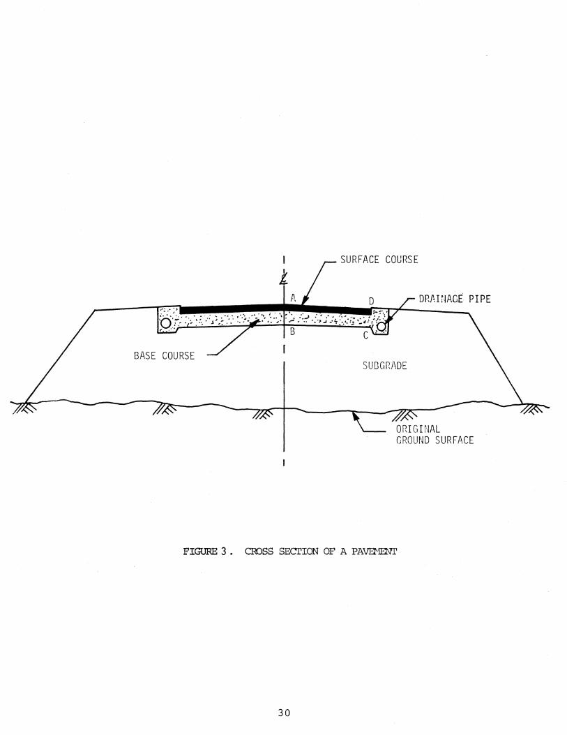
Excess water in the base course and subgrade
significantly influences the performance of pavements. The
design of highway subdrainage requires a proper analysis of
the drainage characteristics of base course and subgrade as
indicated in Figure 3.
4.1 CASAGRANDE'S AND SHANNON'S METHOD
The subject of base course drainage
considerable attention over the last
has
three
received
decades.
Casagrande and Shannon (]:) made field observations on
several airfields in the United States to determine the
environmental conditions under which base courses may become
saturated. They performed a simplified theoretical analysis
of the base course drainage. They assumed symmetry along
the axis of the pavement and the equations governing
drainage for one half of the cross section of the base
course layer ABCD (See Figure 4) were developed. In their
analysis, the drainage process was divided into two parts.
In the first part shown in Figure 4, the free surface
gradually changes from position CD to CA due to free
drainage through the open edge CD of the pavement. Darcy's
Law and the continuity equation were satisfied to establish
a relation among time, t and x(t) in terms of H, L, a,
and n 1 as illustrated in Figure 4 • In the
29
I SURFACE COURSE
! D
;b·;f: :-::·:. ... :.:.;.~·:·:· ::·~:··::·· :::-,:· =~ _.·::! .:·.;}_:<:.:,-;;·:.~;{?"::' • ,.... B C •. ·
BASE COURSE SU13GRJ\DE
FIGURE 3. COOSS SECI'ION OF A PA\M1ENT
30
DRJl.HIAGE. PIPE

dx x
~-+-- t A
H
L tan a 8
STAGE l U < 50%
STAGE 2 U > 50%
FIGURE 4 • CASAGR2\NDE-SHANNON M)DEL FOR BASE COURSE DRAINAGE
31

second part shown in Figure 4, the free surface rotates from
position CA to CB due to the loss of water through the face
CD. The subgrade is assumed to be impervious through the
entire flow calculation. In this part, Casagrande and
Shannon (l) established a relation among t and h(t) in
terms of other parameters mentioned previously. Further
details of their development and the drainage equations are
presented in the following section of this paper. The
theoretical results were compared with field observations by
Casagrande and Shannon (l) and the deviations between
theory and field results are primarily due to the
assumptions that the phreatic surface is a straight line and
the subgrade is impervious.
presented Casagrande's and
Later Barber and Sawyer (~)
Shannon's (l) equations in the
form of a dimensionless chart shown in Figure 5. Most
recently Cedergren and Moulton have modified
the original definition of the slope factor, S, as the
reciprocal of the one shown in Figure 5 and have presented
similar drainage charts in their work on highway subdrainage
design.
Drainage of a sloping layer of base course involves
unsteady flow with a phreatic surface. The assumptions by
Casagrande and Shannon (l) lead to the simple model shown
in Figure 4. In this model, the centerline of the base
course, AB, and the bottom of the base course, BC, are
considered as impervious boundaries. Free discharge is
32

0 ..........
0 .__...
w (.!) c=l: z
w ........
w c:r: 0:: 0
LL 0
w w 0::: (.!) w
I
~ 0 h
' ~~ 20
40
60
80
SLOPE FACTOR, S = _H __ L tan a.
tk H TH1E FACTOR, T = --;
n1L
DEGREE OF DRAINAGE, U _ DRAINED AREA
TOTAL AREA
r HORIZONTAL BASE S + oo
1ool_ __ -L----~----~--~~--~~--~~--~----~--~~--~ 0. 01 0.1 1.0
T - TH1E FACTOR
10.0
FIGURE 5. VARIATION OF DRAINAGE AREA WITH SLOPE FACroR AND TIME FACIDR (1).

assumed along the outer edge of the base course, CD. At the
beginning of drainage, the base layer is assumed saturated,
and the face CD is opened instantaneously for free drainage.
In the Casagrande-Shannon model, the phreatic surface is
assumed as a straight line that rotates with time as
illustrated in Figure 4. The problem was solved in two
parts and the solutions were presented in the following
dimensionless form:
(A) Horizontal Bases
Stage l
Stage 2
(B) Sloping
Stage l
Stage 2
in which
0 < u < 50%
T = 2U 2
50% < u < 100%
T - u - 2-2U
Bases
0 < u < 50%
T = 2 us - s2 ln [S+2U] s
50% < u < 100%
T = s + s ln [(2S-2US+l) ]-S2l [S+l] (2-2U) (S+l) n S
Degree of Drainage, U = Drained Area Total Area
H Slope Factor, S = --Ltana
Time Factor, T
34
( 4-l)
( 4-2)
(4-3)
(4-4)

where H = thickness of base course,
L = half width of the pavement,
= slope angle,
= time,
= coefficient of permeability of base
course, and
nl = effective porosity of base course.
The Casagrande-Shannon model has been used extensively
by Barber and Sawyer (~), Cedergren (~) , Markow
and Moulton (~), in the form of a chart shown in Figure
5. However, the theoretical analyses reported by Wallace
and Leonardi indicate that the phreatic surface
assumes a shape closer to a parabolic rather than to a
straight line. Dupuit's assumption as used in related
drainage problems by Polubarinova-Kochina (_!) also
suggested that a parabolic phreatic surface would yield more
realistic results for drainage calculations.
It was noted in the paper by Casagrande and Shannon
that as the slope of the pavement (tan a ) became
flatter or the depth of the base (H) became greater, the
predictions differed more widely from observations. To
account for this difference, Casagrande and Shannon <!>
introduced a correction factor which depended upon these
variables. In addition it appeared that in the actual cases
reported in this paper, the base course took longer to drain
than was predicted by the theory. Because the Casagrande-
35

Shannon theory underpredicts the amount of time that a base
course is wet, which is not conservative especially in the
deeper and flatter pavements, it was considered beneficial
to develop a better means of analyzing the drainage from
base courses.
4.2 PARABOLIC PHREATIC SURFACE METHOD WITH AN IMPERMEABLE
SUBGRADE
In order to compare the effects of an assumed parabolic
phreatic surface relative to the straight line assumed by
Casagrande and Shannon (!) , an impermeable subgrade was
assumed and the resulting drainage equations were developed
{~). Two separate stages were identified as shown in
Figure 6 and the corresponding equations are as follows {see
Appendix B):
{A) Horizontal Bases
Stage 1 0 < u < 1 3 { 4-5)
T = 3U 2
1 < u < 1 3 Stage 2 ( 4-6)
8 1 T = (-)-1 9 1-U
{B) Sloping Bases
Stage 1 0 < u < ! - 3 {4-7)
T = lsu-ls 2 ln[ 5 + 4U] 2 8 s
Stage 2 1 3
< u < 1 (4-8)
T = S 3 2 3S+4 9S-9SU+8 2-ss ln[~]+Sln[3(1-u) (3S+4)]
36

H =dh~
h
L tan a ·
dx x
STAGE 1 0 ~ U ~-§-
STAGE 2
FIGURE 6. TTl MODEL FOR BASE COURSE DRAINAGE WITH AN IMPERMEABLE SUBGRADE
37
t+dt
t
t+dt

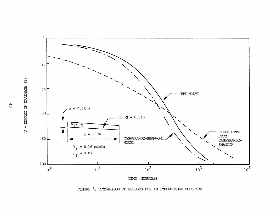
The results of these drainage equations are presented
in the form of a dimensionless drainage chart in Figure 7.
Also, the calculated results from the new model are compared
with field data reported by Casagrande and Shannon (1} on
three of their five pavement test sections in Figures 8 to
10. In the Texas Transportation Institute (TTI} model
drainage proceeds slower than in the Casagrande-Shannon
model, and has roughly the same shape.
The TTI model could be made to fit the field data
results better if drainage were allowed to infiltrate into a
permeable subgrade, thus increasing the initial degree of
drainage and shortening the drainage time.
4.3 ANALYSIS OF SUBGRADE DRAINAGE
In order to study the influence of subgrade drainage on
base course drainage, two models were developed. In these
models the phreatic surfaces in the base course were assumed
to be linear and parabolic. The two distinct stages of
drainage in the first permeable subgrade model are shown in
Figure 11. In this model, the properties of the subgrade
are defined by the coefficient of permeability k 2 , and
porosity, An advancing wetting front, FC, was
assumed at an unknown depth of as shown in Figure
12. Similar to the Casagrande-Shannon model, the drainage
problem begins with a saturated base-subgrade composite
system and the faces EC and DC are opened instantaneously,
38

~------------------------------------------------n ~~
0 0 N
0 1,0
<%) :amtNTh1ia a:o mrc:~a - n
39
0 00
.-t
.-t 0 .-I
0 0 .-I
r-f I 0 .-t
N I 0 .-t
. r--.
,!:..
0
-o\O
~ ~ Q
~
~ 0 I
::J
0~------------------------------------------------------------------------~
-20
40
60
80
---...... ...... ...... ...... ...... ........ ......
..... ' .....
' ' ::. \r=ma '\,
( H = 0.46 m
r tan a == 0.016 - [ kl 1 fl1 ,
Tl J L =23m .... ....
k1 = 0.16 m/min
111 = 0.07
C'!\SAGRANDE-SHAl\INO't-J~ ~DDEL
' ' ~ FIElD DATA V FID.\1
CASAGRAL"'DE-
' ' SHANNON
' ' .......
100------------------L-----------------~----------------~--~~----------~ 10° 101 102 103 104
'I'IME (tmiDI'ES)
FIGURE 8. <:n1!?ARISON OF RESULTS FOR AN IMPERMEABLE SUB~DE

-o\O .._
~ ~ Cl
""" t) I-"
~ ~ I
:::>
0
20 J- CASAGRANDE-SHMl!\lQN IDDEL
40
60
80
FIEID DATA FID1 C..~GRAl'lDE & SHANNON
H = 0.46 m
( r tana~ 0.015
U:1' nl T - , J L = 23m
.....- .. k1 = 9.6 m/min
TI'I tO)EL
n1 = 0.43 100 ~ . ---
10-l 100 101 102
Tll1E (HINUI'ES)
FIGURE 9. CUIP.A.."R.ISON OF PESULTS FOR R~ IHP:Em.mABLE SUBG~.DE
103

0~--------------------------------------------------------------------------~
............ 20 t-
C.1\SAGRZ\NDE-SH."l\!·1NO..lll _I . " M:IDEL - I
""- . ""'-1 Tri lfllEL
o\D
ril t9 40 .a::
~ :.J-- .... " ~ Cl FIELD DATA F'RCl4 .........
.II>- ~ CASAGRANDE & SHA:t-.'N<.JN ,,
N.
~ 60 I (II= 0.8 m ~ Q
,r-tana= 0.01 p I - [k;~:, nJ ;--
-I 80 1- Ti. L = 23m
k 1 = 2.4 m/day \
n1 = 0.04
100- I I I ---10-2 10-1 10° 101 102
TTI·!E (n.zcrs)
FIGURE 10. c:::a-IPARISON OF HESULTS IDR AN IMPERmABLE SUBGRADE

Page 43 missing from original

PHREATIC SURFACE AT TIME t
D
H 8 DRY
WET kl'
E Ltana. c yo(t)
\ / ....... WET F -- - -
K DRY I
'------ WETTING FRONT
FIGURE 12. Definition Sketch For Subgrade Draina~e Model
44

allowing free drainage. In order to keep the model simple,
a one-dimensional flow into the subgrade is assumed in
accordance with Polubarinova-Kochina (!) . From this
formulation the velocity of drainage, v, into the subgrade
is given by (see Appendix C-l):
n = H+_l (H-h(t))
n2
h(t) = depth of water in base course,
(4-9)
(4-10)
y 0 (t) = penetration of water into the subgrade,
k 1 = coefficient of permeability and porosity
of the base course, and
k 2 = coefficient of permeability and porosity
of the subgrade.
The modified differential equations for this model did not
yield a set of dimensionless variables to permit the
preparation of dimensionless drainage charts. Furthermore,
the governing equations were too complex to generate any
closed form solutions. A numerical integration scheme was
used to solve these governing equations.
4.4 DRAINAGE WITH A PARABOLIC PHREATIC SURFACE AND A
PERMEABLE SUBGRADE
The parabolic phreatic surface model, incorporated with
45

the subgrade drainage, is used for subdrainage analysis.
The derivation is listed in Appendix C-2. The model has
the same two stages as were identified earlier in Figure 6
and is illustrated in Figure 13.
Five field cases were studied using this model and the
results for two of these are shown in Figures 14 and 15. It
is interesting to note in Figure 14 that the field curve
follows a trend very similar to that of the two drainage
curves (k 2;k1 = K=0 and 0.0002) given by the present
model and lies between the two theoretical curves. In this
case, the permeable subgrade model with a parabolic phreatic
surface yields results that compare well with field data.
In Figure 15, the parabolic model with a permeable
subgrade (K = 0.0001) is in closer agreement with the field
data than the Casagrande-Shannon model.
As a result of the studies reported here, the parabolic
phreatic surface model with permeable subgrades was chosen
for all future drainage analyses.
4.5 APPLICATION TO PAVEMENT DRAINAGE DESIGN
As an illustration of the importance of subgrade
drainage, a base course 0.8 m (2.5 ft) thick and 46 m (150
ft) wide with l% cross slope is considered. The base course
has its smallest particles in the medium sand range and has
a coefficient of permeability, = 2.4 m/day (7.8
ft/day), and the porosity, n 1 = 0.04. It is required to
46

H
L tan a
STAGE 1
t
H t+c!t
L tan a
STAGE 2
FIGURE 13. SUBGRADE DRAINAGE MODEL WITH PARABOLIC PHREATIC SURFACES
47

,-... "-" "~
LLJ C.. !:I c:( z ...... c:( 0:: Cl
Ll~ 0
""' cx;l l.IJ LLl 0:: (.!} LLl Cl
I
::;::)
0
20
40
60
80
K = 0.0002 ,, FIELD DATA FRO~l _J "' CASAGRANDE & SH.'-\NNON ~
H
i T
k2' n2 L
L = 23 m
H = 0. 5 m
tt.:n a = 0.015
k1 = 9.6 m/min
n1 = 0.43
k2 K = ·-
kl
CASAGRANDE-SHANNON MODEL
100 . lOZ w-1 l.
'I
lOu 101
Tit"1E (MINUTES)
FIGURE 14. RESULTS OF TTI MODEL WITH PERMEABLE SUBGRADES

..........
* ,_
w <..!) c::( z: ........ c::( 0:::: 0
LL 0
""' LLJ
"' w 0:::: <..!) w 0
I
::::>
Or-----------------------------------------------------------------------~
20
40
60
80
100
1 1- I 7
k2' n2
I< = 0.0001 .......
FIELD DATA FRQtc1 CASAGRANDE & SHANNON
L = 23m
.......
k 1 = 7 • 8 m/min
H = 0.15 m n 1 = 0. 4
tan a = 0.015 k,
K = __!:_ k1
.-- CASAGRANDE -SHANNON ~10DEL
~~-------~~--------L----------L~~~ 10-1 10° 101 102
TH1E (r1INUTES)
FIGURE 15. RESULTS OF TTl MODEL WITH PERMEABLE SUBGRADES

determine the drainage time for a 60% degree of drainage for
a number of subgrade materials. Figure 16, for various
values of subgrade permeability, the times required for 60%
drainage can be obtained as follows:
a) Subgrade material is a plastic clay.
kl = 0.0024 m/day (0.0078 ft/day)
K = k2/kl
= 0.001
t = 5 days
b) Subgrade material is a glacial till.
k 1 = 0.0048 m/day (0.0156 ft/day)
K = 0.002
t = 2.5 days
c) Subgrade material is a silty sand.
k 1 = 0.24 m/day (0.78 ft/day)
K = 0.1
t = 84 minutes
It becomes clear, from the above calculations that the
subgrade permeability will significantly influence pavement
drainage and subdrainage design. A specific example is used
here to illustrate the usefulness of the new TTI base-
subgrade drainage model with the aid of Figure 16. More
general pavement drainage design calculations can be
performed by using the computer program "TTIDRAIN" which was
used to make the calculations reported here.
50

o~------------------------------------------------------------------~
L = 23m
H = 0.8 m k1 : 2.4 m/day 1 n1 - 0.04
2
...-. ~
k -2 l
K =- T k1 k2' n2
L ··-w <..!': ::;; ....... "": 0:: 0
LJ_ 0
U1 L.U 1-' LL.I 0:: (!)
6 w 0
I
:::J
8
K = 0.1 _j K = 0.01 _j K = 0.002
K = 0.001
101~----------~~--------------~._ ______________ ._ ____________ ~--------10-1 100 101 102
TH1E (DAYS)
FIGURE 16. DRAINAGE CURVES FOR TTl MODEL WITH PERMEABLE SUBGRADES
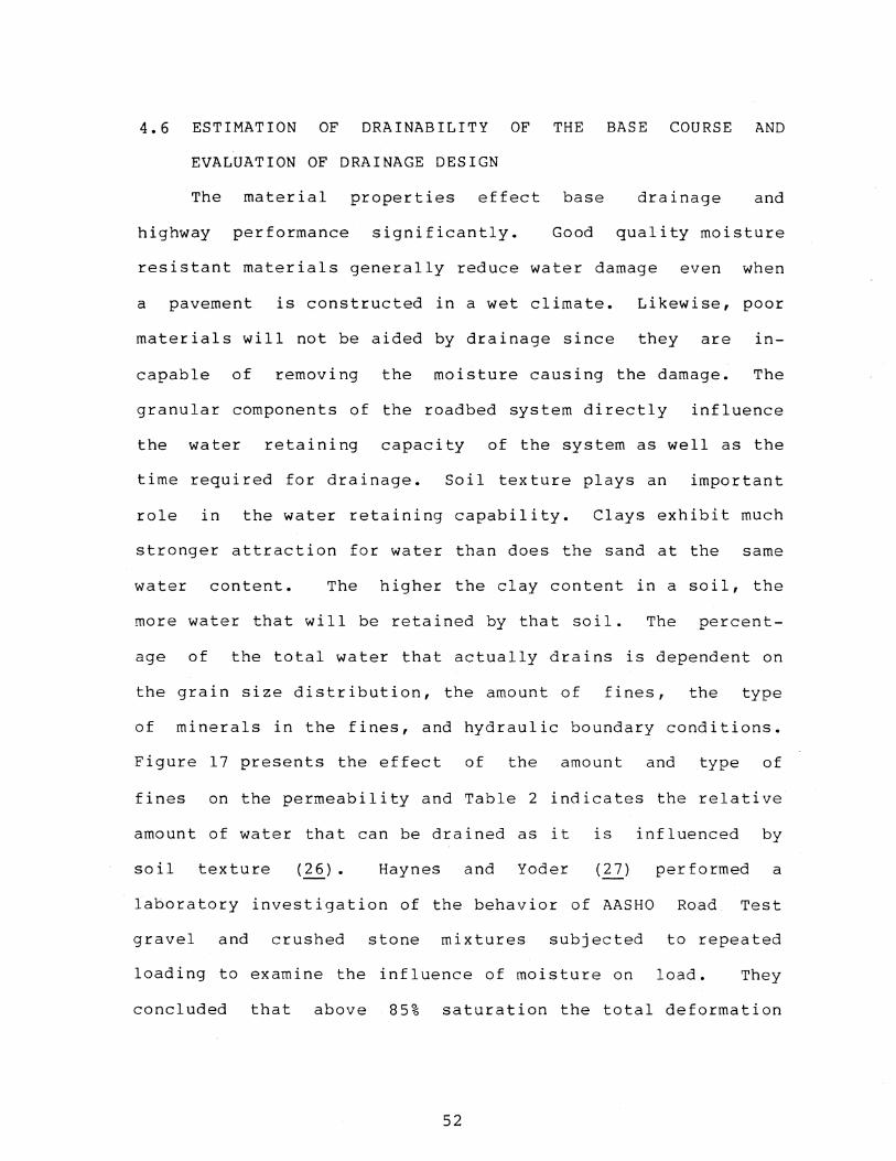
4.6 ESTIMATION OF DRAINABILITY OF THE BASE COURSE AND
EVALUATION OF DRAINAGE DESIGN
The material properties effect base drainage and
highway performance significantly. Good quality moisture
resistant materials generally reduce water damage even when
a pavement is constructed in a wet climate. Likewise, poor
materials will not be aided by drainage since they are in
capable of removing the moisture causing the damage. The
granular components of the roadbed system directly influence
the water retaining capacity of the system as well as the
time required for drainage. Soil texture plays an important
role in the water retaining capability. Clays exhibit much
stronger attraction for water than does the sand at the same
water content. The higher the clay content in a soil, the
more water that will be retained by that soil. The percent
age of the total water that actually drains is dependent on
the grain size distribution, the amount of fines, the type
of minerals in the fines, and hydraulic boundary conditions.
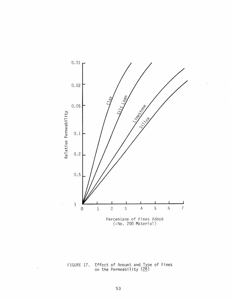
Figure 17 presents the effect of the amount and type of
fines on the permeability and Table 2 indicates the relative
amount of water that can be drained as it is influenced by
soil texture (~). Haynes and Yoder
laboratory investigation of the behavior of AASHO
gravel and crushed stone mixtures subjected
loading to examine the influence of moisture on
performed a
Road Test
to repeated
load. They
concluded that above 85% saturation the total deformation
52
0.01
0.02
0.05 >, +-' •r-.--•r-.0 ttl (1)
E ~ 0.1 (1)
0...
(1)
> •r-+-' ttl
.-- 0.2 (1) 0::
0.5
1 0
FIGURE 17.
1 2 3 4 5
Percentaqe of Fines Added (-No. 200 Material)
6
Effect of Amount and Type of Fines on the Permeability (26)
53
7

U1 .J;::.
AMOUNT OF FINES
TYPE OF I FINES
GRAVEL
SAND
TABLE 2. Drainability (in Percentage) of Water in the Base Courses from a Saturated Sample (~)
<2.5% FINES 5% FINES
INERT INERT INERT FILLER SILT CLAY FILLER SILT CLAY FILLER
70 60 40 60 40 20 40
57 50 35 50 35 15 25 --~
*Gravel, 0% fines, 75% greater than #4: 80% water loss
* Sand, 0% fines, well graded: 65% water loss.
*Gap graded material will follow the predominant size.
10% FINES
SILT CLAY
30 10
18 8

increases thus accelerating fatigue damage. Research done
in New Zealand has shown a degree of base course
saturation of 80% is sufficient to create pore water
pressure build up and associated loss of stability when a
pavement is subjected to repetitive traffic loadings.
The degree of drainage, U, which is employed in the
previous sections of this chapter, can be readily converted
to saturation using Table 2. The relationship between
saturation, S , and the degree of drainage is a
S = l - P.O. x U a (4-ll)
where P.D. is a percentage indicating the amount of water
that can be drained from a sample.
A drainage time of five hours to reach a saturation
level of 85% is set as an acceptable material based on
studies done at Georgia Tech and the University of Illinois
(Figure 18) • A drainage time between 5 and 10 hours is
marginal and greater than 10 hours is unacceptable. A base
course with granular materials that are classified as
unacceptable will hold more water (~), allow excessive
deformations, pumping, stripping, etc., in the pavements.
55

Vl s... ~ 0 :I:
20
15
.. 10 CIJ E ·~ 1-
5
0
Unacceptable
Sati sfactoryl
80 85 90 95 100
Saturation, %
FIGURE 18. Drainage Criteria for Granular Layers (26)
56

CHAPTER 5 EFFECT OF SATURATION ON
LOAD-CARRYING CAPACITY OF
BASE COURSE AND SUBGRADE
For both highway and airfield pavements, benefits
derived from proper drainage cannot be overemphasized. With
excess water in a pavement structure, the damaging action of
repeated traffic loads will be accelerated. Barenberg and
Thompson (~) reported the results of accelerated traffic
tests and showed that rates of damage when excess water was
present were 100 to 200 times greater than when no excess
water was present.
Most pavement design methods use strength tests made on
base course and subgrade samples that are in a nearly
saturated condition. This has been standard practice for
many years due to the fact that the soil moisture content is
usually quite high under a pavement even under desert
conditions.
5.1 EFFECT OF SATURATION ON BASE COURSE PROPERTIES
Moynahan and Sternbert (~) studied the effect of the
gradation and direction of flow within a densely graded base
course material and found that there was little effect on
the drainage characteristics caused by the direction of
flow; however, fines content was found to be a much more
significant factor in determining the rate of highway
57

subdrainage.
As mentioned in Chapter 4, Haynes and Yoder (~)
performed a laboratory investigation of the behavior of the
AASHO Road Test gravel and crushed stone mixtures subjected
to repeated loading. A series of repeated triaxial tests
were performed on the crushed stone and
materials. Their studies indicated
gravel base course
that the degree of
saturation level was closely related to the material
strength of the base course (Figure 19), especially above
85% saturation.
In the simulation model presented here, the moduli of
different base course materials must be furnished. The base
moduli in Table 3 were measured by a wave propagation method
at the TTI Pavement Test Facility (l!) and are provided as
default values to the simulation model. In simulating the
influence of degree of saturation on the base moduli, Figure
19 is applied to determine the ratio of elastic moduli
affected (~). A linear relationship is used to convert
the rate of deflection change to the rate of elastic modulus
change, at different saturation levels. In the range of
degree of saturation from 0 to 60%, the elastic moduli are
assumed to be constant. Between 60% and 85% saturated the
slope between deflection measurements and saturation levels
is 0.24. At
slope is 3.5.
any specific
degrees of saturation greater than 85%, the
To estimate the average base modulus during
season, the cumulative probabilities of each
58

Vl Q)
..c. u s:::
"'0 s::: ::::l 0
..0 Q)
c:::
Vl Q)
..c. u s:::
s::: 0 .,..... +-' u Q)
.--4-Q) Cl
.-ttl +-' 0 I-
0
60
60
LEGEND A 6. 2% Fines 0 9.1% Fines 011.5% Fines ---Gravel
70
----Crushed Stone
70
80 90
80 90
DEGREE OF SATURATION, PERCENT
FIGURE 19. Effect of the Degrees of Saturation on the Repeated-Load Deformation Properties of the AASHO Granular Materials (I[)
59
100
100

1.
-2.
3.
4. I
I 5.
6.
7.
8.
TABLE 3. Calculated Elastic Moduli for Materials in the TTI Pavement Test Facility (l!_)
I I Calculated
Materials Unit l Poisson's Elastic Weight, Ratio Modulus lb/ft3
! lb/in2
Crushed Limestone - -
+ 4% Cement 140 0.45 425,300
Crushed Limestone 140 0.45 236,300 +-2% Lime
Crushed Limestone 135 0.45 209,300
Gravel 135 0.47 64,600
Sand Clay 125 0.47 29,800
Embankment - Compacted I I
120 0.48 I 17,100 Plastic Clay I
I Subgrade 15,000 I
Asphalt Concrete I
500,000
60
section of the elastic modulus as well as the dry and wet
probabilities of the base course (see Chapter 6) are
incorporated into the model.
5.2 EFFECT OF SATURATION ON SUBGRADE PROPERTIES
The moisture content of subgrades are significantly
affected by the location of the water table. If the water
table is very close to the surface, within a depth of 20
feet, the major factor influencing moisture is the water
table itself. However, when the water table is lower than
20 feet (~), the moisture content is determined primarily
by the seasonal variation of rainfall. In this report, the
location of the water table is not taken into account.
The subgrade soil support is
design thickness of a flexible
Robnett (ll) conducted research
a major concern in
pavement. Thompson
toward identifying
the
and
and
quantifying the soil properties that control the resilient
behavior of Illinois soils. In their paper, they concluded
that the degree of saturation is a factor that reflects the
combined effects of density and moisture content. The
simple correlation analyses indicated a highly significant
relation between the resilient modulus and the degree of
saturation of the subgrade. A set of regression equations
were developed for various soil classification groups (Table
4). The equations developed can be used to predict the
resilient moduli of different soil groups. The regression
61

TABLE 4. Regression Coefficients for the Effect of Degree of Saturation on Elastic ~1oduli of Subgrade Soils (]]._)
I b I a Group I Horizons Kips
I
I per square inch
(a) AASHO
A-7-5 ABC 39.83 0.453 BC 27.54 0.266
A-4 ABC 17.33 0.158 BC 16.76 0.146
A-7-6 ABC 31.22 0.294 BC 24.65 0.196
A-6 ABC 36.15 0.362 BC 35.67 0.354
1
(b) Unified
CL, ML-CL ABC 31.89 0.312 BC 32.13 0. 311
-
CH ABC 21.93 0.151 BC 23.02 0.161
ML, MH ABC 31.39 0.331 i BC 29.01 0.284 I l
Equation: Es = a - bSa
Es is in kips per square inch; Sa is degree of Saturation as a percentage
62

coefficient b is indicative of moisture sensitivity.
The depth of the base course and subgrade is assumed to
be 70 inches in order to evaluate the degree of saturation
in the subgrade. The average wetting front of water
penetrated from base into subgrade is calculated by
estimating the proportions of water in the base flowing into
the subgrade from the TTI drainage model (see Chapter
4) (25). The average subgrade modulus is determined by the
average rainfall during that season that will infiltrate
into the subgrade from the base.
where
The subgrade modulus is calculated by (i!)
E s
E = calculated total subgrade modulus, s
d = depth of subgrade,
(5-1)
= subgrade modulus under 100% saturated
condition, which is evaluated from Thompson
and Robnett equations (ll),
= average depth of water penetrating into
subgrade from the base course,
E2 = subgrade modulus under dry condition, and
d 2 = average depth of dry portion of the subgrade.
63
CHAPTER 6 SYNTHESIS OF THE METHODS OF RAINFALL
INFILTRATION, DRAINAGE, AND LOAD-CARRYING CAPACITY
OF A PAVEMENT
The following models are presented to serve as
analytical procedures of rainfall infiltration, drainage
analysis, and load-carrying capacities of base courses and
subgrades.
l.
2 0
3 0
4 0
5.
The Gamma distribution
distribution.
Dempsey and Robnett's
for the rainfall amount
regression equations, as
well as Ridgeway's (l!) field test results from which
an estimation of the amount of rainfall which, in turn,
permits an estimate of the duration of the rainfall,
for infiltration analysis.
The TTI drainage model (_e) , which uses a parabolic
phreatic surface and permits subgrade drainage, was
developed for base course and subgrade drainage
analysis.
Markov Chain Hodel (]_,l:.?_) and Katz's recurrence
equations for the calculation of dry and wet
probabilities of the weather and the base course.
Evaluation of base course and subgrade moduli
as they are affected by moisture contents
in the materials.
64
A conceptual flow chart is drawn in Figure 20 to give a
clear profile of the entire model, and a synthesis of the
various models mentioned above into n systematic analysis of
the rainfall, infiltration and drainage analysis of a
pavement is sketched in Figure 21.
6.1 CONCEPTUAL FLOW CHART FOR RAINFALL, INFILTRATION AND
DRAINAGE ANALYSIS
The local rainfall frequency during a period of time is
used to predict the chances of a given day being wet or dry
by using a Markov chain model. The rainfall amount on every
rainy day during this time period is for estimating the
parameters of a Gamma distribution, which is applied as a
probability density function of rainfall quantity.
The amount of water penetration into the base through
cracks and joints is estimated either by Ridgeway's
laboratory results or by Dempsey-Robnett's regression
equation, which depend on whether the data of cracks and
joints are provided.
Drainage analysis is based on the TTI model, which
determines the time required for water to flow both
laterally out of a base course and simultaneously into the
subgrade. Also, the design of the base course drainage is
evaluated by classifying it as satisfactory, m3rginal, and
unacceptable using criteria established by Carpenter,
Darter, and Dempsey (~).
65

A. Rainfall
Rainfall Frequency
--------~ .. ~ "larkov Chair ----l ... ~ Method
Dry & Wet Probabilities - -I
.._ ____ _
Rainfall Amount
B. Water Infiltration
Cracks & Joints Data
No
Yes
Gamma Distribution
Dempsey's Field Test (Regression
Analysis)
idgeway's Lab esults (Infil ration Data)
t flater Amount in Pavement
C. Drainage Analysis -- ---- ------ --- _j
Parabolic free surface & sub-grade drainage
+ I
Base Course Properties
' Base Drainage I Design Evalu-
ation
I __ _. I Average ·-r--- --• tl. o2.1 i drainage time
I to.s
Base satur-ation Distri-but ion
l ..._.. ____
Base wet Probability
• Base & Subgrade
Elastic Moduli
FIGURE 20. Flow Chart for Conceptual Model of Rainfall Infiltration and Drainage Analysis of Pavements
- J

PRECI PI TAT ION DATA
J~ GAMMA DISTRIBUTION l
1~ )I
Rainfall Amount (Ri)
H INFILTRATION ANALYSIS I '
Degree of Saturation (Sai)
~ Degree of Drainage (Ui)
H_DRAINAGE ANALYSIS
Drainage Time (Ti)
~ MARKOV CHAIN MODEL KATZ'S EQUATIONS
' Dry Probabilities for Corresponding
Drainage Time W(O; Ti )
'
~ 1 I 1
• I 2 3 Ti
Dry Probability for a base= Lpj·W(O·,Til
FIGURE 21. Synthesis of Models Used in Systematic Analysis of Rainfall Infiltration and Drainage Analysis of a Pavement
67

Katz's recurrence equations which are
associated with the Markov chain model, together with the
gamma distribution for the quantity of rainfall, the
infiltration of water into the base course and the drainage
analysis, are applied to estimate the probability of a base
course remaining dry or wet. After taking the climatic
condition, water penetration and drainage design of a base
course into consideration, the distribution of various
saturation levels in a base and a subgrade is then used for
predicting the elastic moduli of these pavement layers.
6.2 SYNTHESIS OF THE METHODS OF RAINFALL MODEL,
INFILTRATION AND DRAINAGE ANALYSIS
Figure 20 indicates that a gamma distribution is used
to fit the quantity of rainfall distribution, and the rate
of infiltration of rainfall into a pavement is estimated
using Ridgeway's field test data. The model for the
estimation of the duration of rainfall provides the
calculation of the amount of water and the degree of
saturation in a base course. If the data on cracks ~nd
joints are not available, Dempsey and Robnett's ( 2 0)
regression equation is used.
The computation of the time required to drain all
excess water out of base courses uses the TTl drainage
model. This model furnishes the relationship between
drainage time and degree of drainage. The degree of
68

drainage directly corresponds to the degree of saturation
which is related to the gamma distribution of rainfall and
to the rainfall infiltration analysis. That is to say, the
probability of having a particular amount of rainfall is
given by
degree of
the gamma distribution, is converted into the
saturation with the aid of infiltration analysis,
and the degree of saturation is used to estimate the time
required for draining excess water out of the base courses
with the TTI drainage model.
As a result, the amount of rainfall is transformed
the corresponding drainage time in terms of days.
into
This
transformation is not linear due to the fact that the
drainage curves of the TTI model are approximately a reverse
S shape (see Chapter 4), while the conversions of the amount
of rainfall into a degree of saturation and further into a
degree of drainage are linearly correlated. In spite of
this nonlinear relation between the amount of rainfall and
the drainage time, the gamma distribution is used to
estimate the probability of requiring a given amount of time
in days to drain out a specified amount of water that
infiltrates. This estimate of the probabilities of having a
specific required drainage time is found by integrating the
areas under the Gamma distribution curve between 0 to 1, 1
to 2, 2 to 3 days, etc.
Once those probabilities of requiring drainage periods
(dry periods) of a specific length in order to remove water
69

from a base course down to a specified level of water
saturation are known, the probabilities of having
consecutive dry days during which the drainage can occur can
be computed by the Markov chain method and Katz's recurrence
equations. The multiplication of the probability of a
required drainage period and the corresponding probability
of actually having that dry period gives the probability of
a base course being dry at the specified saturation level.
BCd = p, X ry 1 w (0;Ti) for tl. 0 > 1 ( 6-1)
where
BC = the probability of a base course being dry,
P. = the cumulative probability of required 1
drainage time from i-1 days to 1 days, which
is corresponds to a certain degree of water
saturation,
W(0;T.) = the probability of m consecutive dry days l •
1 1
from Katz's model (l-2_) ' and
the time, in days, required to drain 100% of
free water from a base course.
While for t 1 _0 <1, i . e. , all the free water can be
drained from a base course within one day, the following
equation is applied
(6-2)
where
BCdry and t 1 . 0 defined as in Equation 6-1.
Pwet = the probability of wet days in the season
concerned, and
70

= the time, in days, required to drain 50%
free water from a base course, which
considered as the average draining time.
of
is
Equation 6-2 is substituted for Equation 6-l whenever it
takes less than one day to drain all free water from a base
course after it is fully saturated by rainfall. This is due
to the fact that Katz's model is incorporated in Equation
6-l in calculating the probabilities of consecutive dry
days, and it is only on a daily basis, which is considered
inadequate for estimating the dry probability for a base
course when all the free water is drained within 24 hours.
For example, there is no difference in estimating the
probability of one base course being dry which takes one
hour to drain 100% of the free water and the same
probability of another base course which takes 24 hours to
reach a dry state.
Two assumptions are made for Equations 6-l and 6-2,
(l) Entrance of free water from rainfall into the
pavement is instantaneous,
(2) No two raining periods occur on any single dry day
when t 1 . 0 is less than one day.
In summary, as a result of these calculations, the
probability of having a dry base under local weather
conditions may be evaluated by Equations 6-l for t 1 _0 >l
and Equation 6-2 for t 0 _ 1~l, respectively.
The average base course modulus for a pavement is
71

computed by incorporating into the analysis the wet
conditions in a base due to the precipitation, the material
strength of the base course affected by different saturation
levels, and the dry-wet probabilities of that base course.
Since the rainfall amount is converted into the saturation
level, the corresponding material strength may be calculated
by using Haynes and Yoder's
The average base modulus
(~) laboratory test results.
under wet conditions can thus be
estimated by finding the average for the gamma distribution.
Furthermore, because the probability of having a wet base
is known as mentioned above, and because the base course
material maintains its full modulus under dry conditions,
consequently the average base course
computed.
modulus may be
A series of sample calculations from the computer
program are listed in Tables 5-9. The rainfall data are for
Houston
pavement
Intercontinental Airport for May 1970, and a
structure is assumed for illustration.
pavement is 100 feet wide on one side, the base course
inches thick, and the subgrade is permeable. Table 5
The
is 6
shows
the degree of drainage and the draining time under the given
base materials by using the TTI drainage model. The
evaluation of a drainage design (~) is presented
6.
in Table
Based on the weather data and pavement structure, the
drainage time, degree of drainage and corresponding
72

TABLE 5. TTl DRAINAGE MODEL FOR AN ANALYSIS OF A HOUSTON PAVEMENT
Problem Number 1 -- Analysis of Houston Pavement in May 1970.
System Analysis of Rainfall Infiltration and Drainage
Length 50.00
Height 0.50
Slope% Perm.1 Perm.2 Poro.1 1.50 10.00000 0.00100 0.2000
(1, 2 stand for base course and subgrade, respectively)
Poro.2 0.0500
Note: The following analysis is based on parabolic phreatic surface plus subgrade drainage
Drainage % Hours 5.0 0.202E 00
10.0 0.760E 00
15.0 0.165E 01
20.0 0.282E 01
25.0 0.426E 01
30.0 0.595E 01
35.0 0.788E 01
40.0 0.101E 02
45.0 0.125E 02
50.0 0.151E 02
55.0 0.198E 02
60.0 0.256E 02
65.0 0.323E 02
70.0 0.403E 02
75.0 0.499E 02
80.0 0.620E 02
85.0 0. 779E 02
90.0 O.lOOE 03
95.0 0.137E 03
100.0 0.187E 03
73
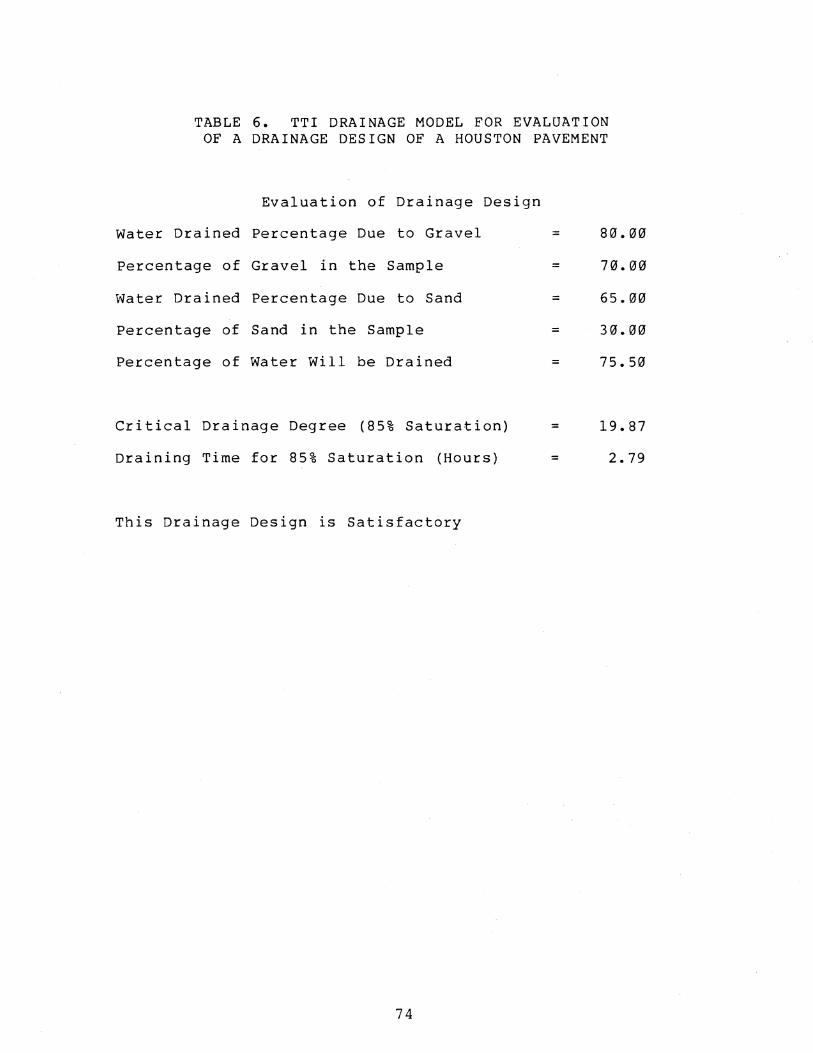
TABLE 6. TTI DRAINAGE MODEL FOR EVALUATION OF A DRAINAGE DESIGN OF A HOUSTON PAVEMENT
Evaluation of Drainage Design
Water Drained Percentage Due to Gravel = 80.00
Percentage of Gravel in the Sample = 70.00
Water Drained Percentage Due to Sand = 65.00
Percentage of Sand in the Sample = 30.00
Percentage of Water Will be Drained = 75.50
Critical Drainage Degree (85% Saturation) = 19.87
Draining Time for 85% Saturation (Hours) = 2.79
This Drainage Design is Satisfactory
74

probabilities are calculated in Table 7. Table 8 gives the
characteristics of gamma distribution and related material
properties under local rainfall conditions, and Table 9
shows the rainfall effect on the base and subgrade moduli.
5.3 DATA REQUIRED FOR ANALYSIS AND SAMPLE RESULTS
The following data should be provided by the users of
the computer program listed in Appendix E that has been
written to make these calculations. Default values for
certain of the parameters are incorporated in the program.
(A) Simulation Model (see Appendix E-3)
(1) Field data for the base course and subgrade, which
include: the half width, height, slope (%), as
well as coefficients of permeability and porosity
of base course and subgrade, respectively.
( 2) Evaluation of base drainage design, input the
percentage of fines (e.g.' <2.5%, 59-0 ' 10%) ' types
of fines (e.g.' inert filler, silt, clay) and
percentage of gravel and sand in the base (see
Table 2) •
( 3 ) Pavement structure and materials data, \vh i ch
include the total area of cracks and joints, the
pavement type (portland cement concrete or asphalt
concrete), base materials (Table 3), the soil type
and horizon of subgrades (Table 4), and total
length surveyed.
75

TABLE 7. MARKOV CHAIN MODEL AND KATZ'S RECURRENCE EQUATIONS FOR DRY PROBABILITIES VERSUS
A DRAINAGE CURVE OF A HOUSTON PAVEMENT
Time (days) Drainage (%) Prob (Consecutive Dry Days)
1 58.72 0.710
2 74.08 0.554
3 83.32 0.432
4 89.17 0.338
5 98.02 0.264
6 95.57 0.206
7 97.30 0.161
8 100.00 0.125
76

-...J -...J
TABLE 8. Stochastic Models for a System Analysis of Rainfall Infiltration and Drainage Analysis of a Houston Pavement
Parameters of Gamma Distribution and Markov Chain Model
Rainfall Average Per Wet Day (inches) = 1.649 Variance of Rainfall Amount = 2.341
Alpha of Gamma Distribution = 1.161 Beta of Gamma Distribution = 0.704
Lamda of Dry Days (Markov Process) = 0.409 Lamda of Wet Days (Markov Process) = 1.000 Sum of Lamda of Dry and Wet Days = 1.409
Probability of Dry Days = 0.710 Probability of Wet Days = 0.290
Water Carrying Capacity of Base (sq. ft.)= 5.000 Average Degree of Drainage per hour(%) = 3.303 Over a 11 Probability of Saturated Base = 0.225
Dry Probability of Base Course = 0.517 Wet Probability of Base Course = 0.483
(The analysis for water entering pavement is based on Dempsey's Infiltration Equation.)

TABLE 8. Stochastic Models for a System Analysis of Rainfall Infiltration and Drainage Analysis of a Houston Pavement (cont'd)
Probability Distribution of Modulus of Base Course
Saturation Level (%) 10 20 30 40 50 60 70 80 90 100
Water in Base (sq.ft.) 0.50 1.00 1.50 2.00 2.50 3.00 3.50 4.00 4.50 5.00
Rainfall Qt. (inches) 0.19 0.44 0.69 0.94 1.19 1.44 1.69 1. 94 2.19 2.44
Rain Duration (hours) 0.00 0.06 0.35 1. 21 3.09 6.62 12.54 21.76 35.31 54.37
Base Moduli (ksi) 64.60 64.60 64.60 64.60 64.60 64.60 29.36 19.00 5.07 2.14
-...] Ratio of Dry Modulus 1.00 1.00 1.00 1.00 1.00 1. 00 0.45 0.29 0.08 0.03 00
Subgrade Moduli (ksi) 29.61 27.99 26.36 24.69 22.97 20.05 16.70 12.75 7.68 1.52
Probability Density 0.48 0.46 0.41 0.37 0.32 0.27 0.24 0.20 0.17 0.15
Probability 0.08 0.12 0.11 0.10 0.09 0.07 0.06 0.05 0.05 0.04
Cumulative Probability 0.08 0.20 0.31 0.41 0.50 0.57 0.63 0.69 0.74 0.78

TABLE 9. EVALUATION OF RAINFALL EFFECT ON PAVEMENT PERFORMANCE OF A HOUSTON PAVEMENT
Distribution Characteristics of Rainfall Effect
Average Free Water in Base (Sq Feet) = l. 07
Duration of Average Rainfall Amount (Hours) = 0.08
Average Rainfall Amount Per Day (Inches) = 0.479
Average Base Course Modulus in Wet State (ks i) = 41.45
Average Base Course Modulus ( ks i) = 53.41
Average Subgrade Modulus (ks i) = 27.30
79

( 4)
( 5)
Climatic data, which include:
period, rainfall amount
(precipitation~ 0.01 inch)
intended evaluation
of every rainy day
during that season,
and the sequential number of wet and dry days.
The weather parameters which depend on the
locality, k, x, n and shape factor
2. The default values for these
(SF) in Chapter
parameters in
order are 0.3, 0.25, 0.75 and 1.65, respectively.
The printout of the program mainly consists of four
parts.
(l) Drainage analysis with TTl drainage model,
(2) Evaluation of the drainage design, the output
evaluates the drainage design to be one of the
( 3)
three categories:
satisfactory;
unacceptable, marginal, and
Parameters of the climate, the alpha (a) and beta
( S) of the Gamma distribution, the wet and dry
probabilities of the weather and the base course
from the Markov chain model and Katz's recurrence
equations,
(4) The probability density distribution and averages
of the base course and subgrade moduli due to the
distribution of saturation levels.
(B) Low Permeability Base Courses Model.
( l) Input the data of each crack width and depth, the
coefficients of horizontal and vertical
80

permeability, respectively, porosity of the base
course and the capillary head in order to estimate
the rate and depth of water penetration into the
base course.
(2) The suction of atmosphere, the initial suction of
base course, diffusion coefficient, ratio of water
content and suction and evaporation constant to
calculate the rate and the amount of water
evaporated from the base course.
The output gives:
(l) The horizontal and vertical distances which water
flows at different times and the depth of water
remaining in the crack.
(2) The distribution of suction at different times and
different soil depths.
(3) The amount of water evaporated from the base
course at different times.
6.4 AN EXAMPLE OF SYSTEMATIC ANALYSIS OF RAINFALL
INFILTRATION, DRAINAGE,
PAVEMENTS
AND LOAD-CARRYING CAPACITY OF
The following conclusions result from a case study of
the effects of rainfall amount and subgrade drainage on the
load-carrying capacity of a pavement. It is assumed that a
base course is 70% gravel, 30% sand, 100 feet wide, 6 inches
deep, 1.5% slope, the coefficient of permeability of the
81

base course is 10 feet per hour, and the porosity is 0.1,
and the subgrade is assumed to be impermeable. The drainage
design used is considered marginally acceptable in terms of
the drainage time of 6.35 hours required to reach a less
than 85% saturation level in the base.
In two climatic regions this same design for a base
course is used. Abilene and Houston, Texas, represent low
and high rainfall areas, respectively. Daily rainfall data
from 1970 were entered into the simulation model to compare
the results for these cities. The results (Figure 22) show
that the precipitation quantity affects the elastic moduli
of the base course. If the water in the base course can
drain into the subgrade with a permeability of 0.01 ft/hour
and a porosity for freely draining water of 0.01 in a higher
rainfall area, i.e. Houston, the load-carrying capacity can
be improved significantly.
82

V'l Q)
-'= u c
.. +-' c ::::l 0 E
c:(
,...... ,...... ro
'+-c ro 0:
>, ,...... -'= +-' c 0 ~
Q) (/')
ro CQ
5
0
Houston FAA Airport
---- Abilene WB Airport
__ .... .... ..... " ... ..... ""
Jan Feb Mar Apr May Jun Jul Aug Sep Oct Nov Dec
Houston Pavement w/Subgrade Drainage Abilene Pavement Houston Pavement
::::---· --. --· _-:r·-·--·------ ------ ----. / ', . --- ..... ""'
Feb ~1ar Apr May Jun Jul Aug Sep
_ . ........---.· I
I
Oct Nov
FIGURE 22. Effects of Rainfall Amount and Subgrade Drainage on Load-Carrying Capacity of Pavements
83
Dec

CHAPTER 7 CONCLUSIONS AND RECOMMENDATIONS
A systematic analysis is constructed which incorporates
a probability distribution of the amount of rainfall,
the probabilities of dry and wet days, water infiltration
into pavements, drainage
carrying capacities of
analysis of pavements, and load
base courses and subgrades. The
simulation model presented herein is a major advance over
other methods that have been used previously for the same
purpose.
The new method has been developed for computing the
drainage of the pavement base and subgrade models using a
parabolic phreatic surface and allowing drainage through a
permeable subgrade. A model of water penetration into low
permeable base courses is also constructed.
This comprehensive analysis of the effect of rainfall
on pavement structures, is recommended as an effective
approach to evaluate design
overlay construction and to
effects on pavements.
84
criteria for pavement and
estimate future environmental

REFERENCES
1. Casagrande, A. and Shannon, W. L., "Base Course Drainage for Airport Pavement," Proceedings of the American Society of Civil Engineers, Vol. 77, June, 1951.
2. Cedegren, H. R., "Drainage of Highway and Airfield Pavements," Wiley, New York, 1974.
3. Markow, M. J., "Simulating Pavement Performance Under Various Moisture Conditions," TRB, Transportation Research Record, 849, 1982, pp. 24-29.
4. Polubarinova-Kochina, P. Ya., "Theory of Ground Water Movement," Translated by J. M. Roger De Wiest, Princeton University Press, New Jersey, 1962.
5.
6.
7.
8.
Kottegoda, K. T., "Stochastic Technology," Wiley, New York, 1980.
Water Resources
Suzuki, E., "Hyper-Gamma Distribution to Rainfall Data," Papers in Geophysics, 15, 1964, pp. 31-35.
and Its Fitting Meteorology and
Suzuki, E., "A Summarized Review of Distributions Fitted to Climatic Factors Chain Models of Weather Sequences, with Some Statistical Climatology, Elsevier, Netherlands, 1980, pp. 1-20.
Fair, G. M., Geyer, J. C., and Okum, D. A., Wastewater Engineering," Vol. 1, Water Wastewater Removal. Wiley, New York, 1966.
Theoretical and Markov Examples," Amsterdam,
"Water Supply
and and
9. Linsley, R. K., Jr. and Franzini, J. B., "Elements of Hydraulic Engineering," McGraw-Hill, New York, 1955.
10. Kazmann, R. G., "Modern Hydrology," Harper and Row, New York, 1965.
11. Am. Soc. Ci v. Eng., "Hydrology Handbook," Manual of Engineering Practice, No. 28, 1949.
12. Gabriel, K. R. and Neumann, J., "A Markov Chain Model for Daily Rainfall Occurrence at Tel Aviv," Quart. J. Roy. Met. Soc. 88, 1962, pp. 90-95.
13. Katz, R. w., "Computing Probabilities Associated with the Markov Chain Model for Precipitation," Journal of Applied Meteorology 13, 1974, pp. 953-954.
85

14. Ridgeway, H. H., "Infiltration of Water Through the Pavement Surface," TRB, Transportation Research Record 616, 1976, pp. 98-100.
15. Ring, G. W., "Drainage Structures," Proceedings of on Concrete Pavement Design, Lafayette, Indiana, 1977.
of Concrete Pavement International Conference
Purdue University, West
16. Woodstrom, J. H., "Improved Base Design for Portland Cement Concrete Pavements," Proceedings of International Conference on Concrete Pavement Design, Purdue University, West Lafayette, Indiana, 1977.
17. Barksdale, R. D. and Hicks, R. G., "Drainage
18.
Considerations to Minimize Distress at the Pavement-Shoulder Joint," Proceedings of International Conference on Concrete Pavement Design, Purdue University, West Lafayette, Indiana, 1977.
Dempsey, B. J., Darter, M. I., and Carpenter, "Improving Subdrainage and Shoulders of Pavement-State-Of-The-Art," University of Urbana, Interim Report, 1977.
S. H., Existing
Illinois,
19. Darter, M. I. and Barenberg, E. J., "Zero-Maintenance Pavements: Results of Field Studies on Performance Requirements and Capabilities of Conventional Pavement Systems," FHWA Report, FHWA-RD-76-105, 1976.
2 0. Dempsey, B. J. Precipitation, Drainage," TRB, 19 7 9' pp. 13-2 3.
and Robnett, Joints, and Transportation
Q. L.' Sealing Research
"Influence of on Pavement
Record 705,
21. Mitchell, P. W., "The Structural Analysis of Footings on Expansive Soil," K. W. G. Smith & Associates Research Report No. 1, Adelaide, Australia, 1980.
22. Barber, E. S. and Sawyer, C. L., "Highway Subdrainage," Public Roads, Vol. 26, No. 12, 1952.
23. Moulton, L. K., "Highway Subdrainage Design," FHWA Report, FHWA-TS-80-224, 1980.
24. Wallace, K. and Leonardi, F., "Theoretical Analyses of Pavement Edge Infiltration and Drainage," James Cook University, Australia, Department of Civil Engineering, Research Report 6, 1975.
25. Liu, S. J., Jeyapalan, J. K, and Lytton, R. L., "Characteristics of Base and Subgrade Drainage of Pavements," Sixty-Second Annual Transportation Research Board Meeting, 1983.
86
26. Carpenter, s. H., Darter, M. I., and Dempsey, B. Pavement Moisture Accelerated Distress Identification System," Vol. 2, FHWA FHWA-RD-81-080, 1981.
J., "A (MAD)
Report,
27. Haynes, J. A. and Yoder, E. J., "Effects of Repeated Loadings on Gravel and Crushed Stone Base Materials in the AASHO Road Test," Highway Research Record 19, 1963, pp 0 8 2-9 6 0
28. Martin, G. R. and Toan, D. V., "Effect of Saturation on Pavement," Proceedings Symposium, Vol. 2, 1971, pp. 486-491.
Base of
Course Roading
2 9. Barenberg, E. J. and Thompson, 0. 0., "Behavior and Performance of Flexible Pavements Evaluated in the University of Illinois Pavement Test Track," Highway Engineering Series No. 36, Illinois Cooperative Highway Research Program Series No. 108, 1970.
30. Moynahan, T. J., Jr. and Sternberg, Y. M., "Effects on Highway Subdrainage of Gradation and Direction of Flow Within a Densely Graded Base Course Haterial," TRB, Transportation Research Record 497, 1974, pp. 50-59.
31. Lytton, R. L. and Michalak, C. H., "Flexible Pavement Deflection Equation Using Elastic Moduli and Field Measurements," Research Report No. 207-7F, Texas Transportation Institute, Texas A&M University, College Station, Texas, August, 1979.
32. Yoder, E. J. and Witczak, M. W., "Principles Pavement Design," 2nd ed., Wiley, New York, 1975.
of
33. Thompson, M. R. and Robnett, Q. L., "Resilient Properties of Subgrade Soils," Transportation Engineering Journal, ASCE, 1979, pp. 71-89.
34. Taha, H. A., "Operations Research 2nd ed.," MacMillian, New York, 1976.
87

APPENDIX A
Rainfall Amount Distribution, Rainfall Duration
and Markov Chain Model
A-1. RAINFALL AMOUNT DISTRIBUTION
Among the theoretical distribution models of
precipitation, the Gamma distribution has a long history as
a suitable model for frequency distributions of
precipitation. The probability density function of the
Gamma distribution is:
where
Sa -SR a-1 f(R;a,(3) = f(a) e R
0
R>O
R<O
R = precipitation amount and
f(a) =Gamma function where (n+l)=n! n=0, 1, 2,
The parameters and may be estimated by
moments method:
-a = R = mean = LRi/n
2 n - 2 S =variance= E(Ri-R) /n
88
(A-1)
the
(A-2)
(A-3)

A-2. RAINFALL DURATION
In Ridgeway's laboratory tests (1:._!), he concluded
that rainfall duration is more important than rainfall
intensity in determining the amount of free water that will
enter the pavement structure. The relation between rainfall
intensity, i, and duration, tR' has often been expressed
in the intensity-duration-recurrence period equation, (~)
where
t p
i
l ktpx
t n R
is the
minutes,
effective rainfall duration
is the recurrence interval in years,
(A-4)
in
is the maximum rainfall intensity, inches per
hour, during the effective rainfall duration,
and
k, x, and n are constants which depend on the locality.
For instance, in the eastern United States, n averages about
0.75 and x and k are about 0.25 and 0.30, respectively. It
is assumed that the relation between rainfall intensity and
time is a Gaussian curve (Figure 1).
Using the standard normal distribution, a rainfall du-
ration, tR, was chosen from -1.96 to 1.96 which made the
area under the curve to be 0.95. Furthermore, i corresponds
89

to 0.3989 in the standard normal distribution curve.
Therefore, the ratio between the product
total amount of rainfall during effective duration, R, is
3.92 X 0.3989 0.95 = 1.65
which is called the shape factor (SF).
(A-5)
The next step is to derive the formula for rainfall
amount, R, and effective rainfall duration, tR, from the
intensity-duration-recurrence equation:
R =
= (tR) (ktpx)/(tRn) (SF)
= kt (l-n)t x/(SF) R p
Thus, tR
1
R(SF) 1-n = ( X ]
ktp
(A-6)
(A-7)
The constant for shape factor (SF) could be determined
and entered by the user (for example, 1.0 for uniform
distribution and 1.5 for parabolic curves).
In the computer programs, the users are allowed to choose
the constants n, x, k, and shape factor. In the meantime,
the default numbers have been set up to be 0.75, 0.25, 0.30,
90

and 1.65, respectively.
A-3. Markov Chain Model for a Time Sequence of Weather
Observation
A transition probability matrix generated from the
Markov chain method for predicting weather sequences is
represented by four elements, represented by the
probabilities given in the matrix below. The matrix is
known as a "transition" matrix.
p ( t) = [p. ·(t)] = lJ
Poo(t}
(A-8)
where p.. represents the probability that the Markovian lJ system is in state j at the time t given that it was in
state i at time 0; the subscript 0 stands for dry, and a
subscript of 1 for wet. Thus p 10 (t) represents the
probability of having a dry day at time t when time 0 is a
wet day, and other elements of this matrix can be
illustrated in a similar manner.
The transition probability matrix of the Markov chain
model is derived from the assumption that the sequence of
events, i.e., wet and dry days, is a negative exponential
distribution.
91

x > 0, > 0, and
f(x) = Ae-).x
x = wet or dry days (A-9)
The variable A is the reciprocal of the average dry or wet
days per period,
where
-X dry
-X wet
1 x .dry
1 x wet (A-10)
= the average number of dry days in a given
period
= the average number of wet days in that same
period.
So that the transition matrix is derived as (i!)
p ( t) = 1
A [1-e-(Aw+Ad)t] d
(A-ll)
Associated wittl the Markov chain model given above is a
recurrence relation for computing the probabilities of dry
and wet days which was applied by Katz (~).
= [::: ::~] X [W0 (k;N-l) l w1 (k-l;N-lj(A-12 )
Transition Matrix
where
= the probability of k wet days during N
consecutive days when the zero-th day is
92

dry (the subscript 0 stands for the
zero-th day equals dry and the subscript
1 stands for the zero-th day equals wet,
and the transition matrix is derived from the Markov chain
method (Equation A-11). Since the recurrence relation is on
a daily basis, the time t is set at 1 day in the transition
matrix. Also, the probability of occurrence of a given
number of wet days in a period of time is formulated as
(A-13)
where
W(k;N) = the probability of having k wet days during N
consecutive days
P0 = initial probability of having a wet day.
Application of Katz's equations to the Markov chain
model results in finding the probability of having k wet
days out of N consecutive days. In order to have exactly k
wet days out of N, either ( 1) the first day is dry and
exactly k of the remaining N-1 days are wet, i.e.,
W0 (k;N-l), or ( 2) the first day is wet and exactly k-1
of the remaining N-1 days are wet, i.e. , W1 (k-l;N-l)
(Figure 23) • Suppose that the zero-th day is dry, then the
probability of the first day being dry is p00 and the
probability for the first day being wet if p01"
Therefore, when the zero-th day is dry, the probability of
exactly k wet days out of N consecutive days is the
93

(I} W0 (k;N)
' I ,
-0-, I '
I
-'Ci-, I '
» I I I I I I I II II II II
I I , I II II II II II II
For N days= Zeroth day
For N-1 days
Poo
Po1
P1o
pll
' I , I I I I -0- k II I I
II II , I ' II II
' • W0 (k; N-1) 'I( /
I I II {k-1) II II l.t II 1/11 II 11 II/I
' .... W1 (k-1; N-1) .. /
' I , j I II ' -0- k 1 II I I II I
, I ' I II I
' • W0(k; N-1) 'I( /
, ; » ' I I I (k -I) 1 I I I II I I
II I I Ill I II I I II II
' • w1tk-l ;N-1 > .. /
First day N-1 days
Zeroth day N-1 days
FIGURE 23. Definition Sketch of Katz Model
94

probability of the first day remaining dry from zero~th day
{p00 ) multiplied by the probability of having k wet days
of the remaining N-1 days, W0 (k;N-l), plus the
probability of changing from a dry zero-th day to a wet
first day {p 01 ) multiplied by the probability of having
k-1 wet days in the remaining N-1 days, W1 (k-l;N-l); so
that
(A-14)
Similarly, if the zero-th day is wet, the probability of k
wet days out of a sequence of N days is
(A-15)
Equation A-12 is simply a matrix form of Equations A-14
and A-15. The total probability of having k wet days out of
N consecutive days is further dependent on the initial
probability of having a wet day {p 0 of Equation A-13).
95

APPENDIX B
Parabolic Phreatic Surface Drain Models
for Base Courses with Impermeable Subgrades
B-1. Analysis of Horizontal Bases with Impervious Subgrade~
The shape of free water surface is to reamin a parabola
that changes with time throughout the analysis. Two
separate stages are identified and illustrated in Figure 24;
ABCD is the boundary of one-side base and point B is the
origin of this system.
y = lax
a =
Drained Area Hx1
= A' = -3-
The rate of water amount (q) change is
dA . dx dq = n 1 · --dx1 1
(B-1)
(B-2)
(B-3)
The flow from time t to t+dt is computed by means of
Darcy's law
gradient, i, is
width is y;
dq(x) dt
and Dupuit's assumption. The hydraulic
=
~ , and the average flow area per dx
k1iy k . ~ k1
H2 = . y = 2x1 1 dx
96
unit of
(B-4)

D
T LX H
nl,kl
1 I· L ·lc
Stage I. 0 ~ U ~ j
U = Degree of Drainage. n1 = Effective porosity of the base course. k1 = Coefficient of permeability of the base course. t = Time.
Stage I I.
FIGURE 24. Staqes of Parabolic Phreatic Surface in a Horizontal Base
97

Combining Equations B-3 and B-4, a differential
equation can be derived, the solution of which leads to
t = (B-5)
Two dimensionless quantities, introduced by Casagrande
and Shannon (!), are called the degree of drainage (U) and
the time factor (T), respectively:
u = Drained Area Total Area
tk1H T = --2
n 1L
Incorporating T and U (U
1 which is valid for O~U~3
x1 = 3L) into Equation B-5 gives
of horizontal bases.
(B-6)
(B-7)
(B-8)
The second part, Stage 2, of the drainage process,
where the variable parabola has a constant base length L and
a variable height, h, (Figure 24) is developed in a manner
similar to the development of Stage 1.
A' = HL - ~hL (B-9) 3
dq 2 ( B-1 0) = - - n Ldh 3 1
~ k1 2 (B-11) dt = 2L h
98

Combining Equations B-10 and B-11,
n = -4 fh _1_ dh
3 H k h2 1
(S-12)
where th and tH are the elapsed time for the free
surface to hit H and h, respectively. Also
2
th-tH 4 n 1L
(l l) (B-13) = ---3 k1 h H
where tH is the time when the free water surface reaches
the full base length (L) in Stage l. Therefore,
2
tH 1 n1L
and = 3 k 1H I
2 n 1L 4 l) th = (--k1 3h H (B-14)
The final solution can be expressed by incorporating the
dimensionless quantities T and U:
u 1 2h and = - 3H ,
T 8 1 (B-15) = -9(1-U)
which are valid for ~ < u < 1 of horizontal bases.
99

B-2. Analysis of Sloping Bases with Impervious Subgrades
Previously, the authors made an attempt to have the
phreatic surface parabola oriented with respect to the
horizontal axis, which forced a limitation of the model.
The limitation is that it cannot then be used to analyze
pavement sections with a slope factor, S, less than 1,
corresponding to base courses with high slopes (tan a or
large widths (L), or shallow depths of base courses (H).
This is due to the fact that when S<l, the parabolic
phreatic surface may rise above the top of the base course
giving a physic~lly impossible negative degree of drainage.
Thus in the following development, the parabolic free water
surface is described with respect to the lower boundary of
the base course rather than the horizontal axis. Two stages
are identified as shown in Figure 25, where ABCD is the
boundary of one-side base and point B is the origin of this
system.
100
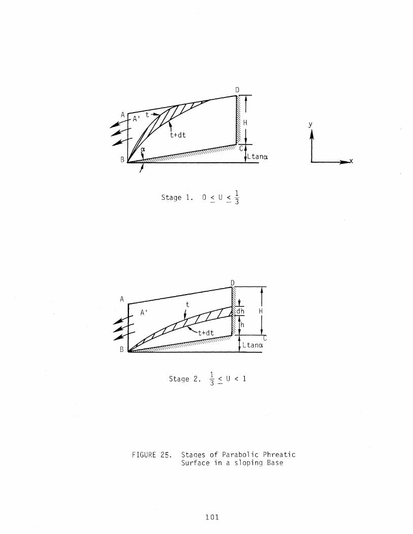
H
Ltana
Stage 1. 0 ~ U ~ ~
Stage 2. ~ ~ U < 1
FIGURE 25. Staqes of Parabolic Phreatic Surface in a sloping Base
101
y
L

y = /ax + X tan a
H2 a =
xl
H rx + tan y = -- X a v'xl
Drained Area 2
(H + x 1 tan a) x 1 xl
tan a A' = - -2-
xl (Vf"/X +X - f tan a)dx 0 xl
H = 3 xl
dA' dq = nl dxl • dxl
Darcy's law~= k 1 i y
Therefore, dq(x) = k 1 (y - x tan a) . iY dt dx
H2 H /X tan a) = k1 (2x1 + ----------/x1
The average rate of flow can be expressed by
~ k1 x1 = f dq (x) dx dt x1 0
2 2 = k1 (_!!__ +
3 H tan a) 2x1
From Equations B-17 and B-18
t X f dt= f 1 0 0
t
Let T = t
x1 [ 4tana
H 3H+4x1tana 2 ln ( 3H ) 1
16tan a
102
(B-16)
(B-17)
(B-18)
(B-19)
(B-20)

Since u x1
and s H = = 3L Ltana
TI 3 su 3 s2 ln (1 + 4U) (B -21) = 2 - 8 s
which is valid for 0 < u < 1 3 of sloping bases -
Stage 2:
y = va:;{ + x tan a
a =
y = + x tan a
Drained Area L
A'= (H + L tan a) L- 1 L2tan a- J 2
Using
= HL - ~ hL 3
dq dA' dh 2 = n1 = - -n Ldh dh 3 1
Darcy's law,
dq(x) = k 1 (y-xtana) ~ dt dx
h 2 htana = k1<2L + ;r rx
2g_ 1 L
dt = L J dq (x) dx 0
k1 h2 ~ h tan a) = ( 2L + 3
103
0
(h ~ t ) dx --+x ana I"L
(B -2 2)
(B -23)
(B -24)
(B -25)

From Equations B-23 and B-24
2 -4 L n 1dh
2 k 1 (3h +4hLtana)
2 H n 1L h = = L\t th-tH k 1Ltana [ ln (
3H+4Ltana 3h+4Ltana
2 hL HL--2 h
Let U 3 1 = = - 3 H HL
L\T = L\t
9S-9US+8 = S ln [3(1-U)(3S+4)]
1 when x 1 reaches L in Stage 1, U = 3
Maximum T = ~ - l s 2 ln ( 3S+ 4 ) I 2 8 3S
) ]
S 3 2 3S+4 9S-9US+8 = 2 8 S ln (~) + S ln [ 3 ( 1-U) ( 3S+4)]
104
(B-26)
(B-27)
(B -28)

APPENDIX C
Parabolic Phreatic Surface Drain Models
for Base Courses with Subgrade Drainage
The influence of subgrade drainage is discussed in this
appendix. In Part C-1 (Figure 26), velocity of water
penetration into the subgrade without side flow from the
base course is evaluated. In Part C-2 (Figure 27),
differential equations for both base and subgrade drainage
are derived. In Figures 26 and 27, ABCD is the boundary of
a one-side base course. Beneath the boundary BC is the
subgrade into which water will penetrate.
of the wetting front in the subgrade are
Different shapes
caused by the
effect of side drainage from the base course. The wetting
front in Part C-1 is parallel to the phreatic surface of the
base, when there is no water flow through the base boundary.
The wetting front in the subgrade of Part B will eventually
reflect the image of phreatic surface in the base. It is
due to the fact that the parabolic shape is created by
base-edge flow and the rest of the water drained is
significantly affected by infiltration into the subgrade.
C-1. WATER PENETRATION INTO THE SUBGRADE FROM A BASE COURSE
The phreatic surface of water which is affected by
lateral drain might be assumed to have any kind of shape.
105

Subgrade
n = porosity k = permeability t = time
0
'T H
1 c
FIGURE 26. Water Penetration into a
y
Suborade without Lateral Drainaqe
106

D ~ r· ~
dh
T y h
t~ E F
FIGURE 27. Water Penetration into a Subqrade with Lateral Drainaqe
107

The parabola drawn here is only to be consistent with the
previous derivations. The datum is located at point 0 in
Figure 26.
The velocity of water is generally defined as
v ~ -k dh (C-1) = = dy dy
h p
(C-2) = - y Yw
<P = vy + c (C-3)
where v is the velocity,
<P is the velocity potential,
h is the total head of water,
k is the coefficient of permeability,
Yw is the unit weight of water,
p is the pressure of water, and
c is a constant.
The velocity potential of the base course and the
subgrade are and ¢ 2 , respectively. Applying
Equations C-1 to C-3 we achieve
¢1 -k p1
y) ' d¢1
= (- - v1 = dy 1 Yw (C-4)
¢2 -k p2
y) ' d¢2
= (- - v2 = 2 Yw dy (C-5)
108

The subscript 1 stands for the parameters of the base
course and 2 for those of the subgrade. At the interface of
the base course and the subgrade (line BC), y=H,
v 1 = v 2 = v, and thus
, and
(C-6)
In order to solve for c1 and c2 in terms of the
parameters which we have been using, two points y=H-h and
y=y 0 (the wetting front) are chosen.
at y=H-h, P=O
~l = -k1 (-y) = k1y = k1 (H-h) = v 1 (H-h)+c1 , so that
c 1 = (H-h) (k1 -v1 ) .
at y=y0 , P=O
~ 2 = v 2y 0+c 2 = k 2y 0 , so that
c2 = (k2-v2>Yo·
(C-7)
(C-8)
Substituting Equations C-7 and C-8 into Equation C-6,
we find the velocity that water penetrates from the base
course into the subgrade:
109

vH+(H-h) (k1-v)
k1
Yo - H+h v =
h y -H + _o_
k1 k2
Furthermore,
determined.
Since v
the
n1 Yo = H + (H-h)
n2
h f
and
wetting front
and
dh, we have
(C-9)
must be
( C-1 0)
which is consistent with the principle of conservation
of mass. Therefore, the velocity of water penetrating into
the subgrade from the base course is
n1 (H-h) + h
n2 (C-11) v =
n1 (H-h)
h + n2
k1 k2
110

C-2. Parabolic Phreatic Surface with Subgrade Drainage
Through the derivations in Appendix B, as well as in
this Appendix, we are aware that the height from base course
boundary to the water surface h (Figure 25) is dependent on
the drainage through the edge line of the base course, to
which we have referenced the parabolic shape. Therefore,
the height is a function of both time and the horizontal
coordinate, x.
Incorporating the lateral and subgrade drainage, the
model is sketched as Figure 28. Point B is the datum.
In Stage 1, the free water surface is parabolic from
the origin to x 1 . From x1 to L, since the lateral
drain has no effect on drainage at time t, the phreatic
surface is parallel to base course lower and upper
boundaries through the subgrade drainage only. In Stage 2,
once the effect of water draining out from the edge line
reaches the width length, L, the whole free water surface
becomes a parabolic shape.
Again, by employing the same techniques used in
deriving the previous equations, the geometry and the rate
of the water quantity draining out are
Stage l
h 2 2 dq 0 h tan a)dt = k1 (2x1 +
X 3 0 (C-12)
dq h2 2 h tan a)dt = k1 (2L + 3 X
Stage 2 (C-13)
111
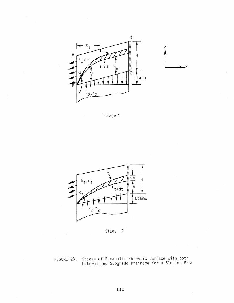
· Stage 1
Stage 2
0
~T H
~ ~+ ~ c Ltana
_!_
y
Lx
FIGURE 28. Stages of Parabolic Phreatic Surface with both Lateral and Subgrade Drainage for a Sloping Base
112

The water quantity flowing through subgrade is
d;ry = n 2dy0 dx
= v rix dt
In Stage 1,
(a) from origin to x 1 ,
v = lax + xtana for ~arabolic free surface
on Figure 28
i) = y -ho
xtana =
dq. (O-x1 ) = v dx dt v
i) (1
= k2
n1 - -)
n2
k2 n1 ~ (-- -)
k1 n2
'<b) from x 1 to L
n + _lH
n2 n
+ _lH n2
n1 n ho (1 - -) + _lH
dxdt
n2 n2 dqy(x1 -L) = dxdt .
k2 n1 n ho (-- -) + _lH
k1 n2 n2
dq Therefore, total _y
dt
n1 n x1 i) (1 - -) + _lH
1 [k2 1 n2 n2
dx = L k2 n1 n1 " 0 y (- -) -F -H
k1 n2 n2
n1 n ho (1 - -) + _lH
+ n2 n2
(L-x )] k2 n1 n 1
ho (-- -) + _lH k1 n2 n2
1 12
(C -14)
( C ·-15a)
(C-15b)
(C -1_6)

In Stage 2,
p =
Total
h
IL
dq ____:_;t_ dt = k2
h L -
J vL h
0 -vL
n1 n rx (1--) + ___!H
n2 n2 (C-17) dx k2 n1 n
rx (---) + ___l_H k1 n2 n2
Similar to the derivation in Appendix I, to combine the
rate of water flow, edge and subgrade drain, and the rate of
drained area change, differential equations for Stages 1 and
2 can be constructed.
dq = dqx + dqy
Stage 1
dq = Equation -x
rt-..- =Equation ~y
C-12
C-15
Runge- Kutta's numerical method is applied to solve
this differential equation.
Stage 2
dq =Equation C -13 X
dq =Equation C -17 y
Simpson's Rule is applied for numerical integration here.
114

APPENDIX D
ENTRY AND EVAPORATION OF WATER IN A
LOW PERMEABILITY BASE COURSE
D-1. WATER ENTRY INTO BASE COURSES OF LOW PERMEABILITY
Free water, mainly due to the rainfall, flows into
cracks and joints of the pavement then penetrates into the
base course. The water infiltration into a low-permeability
base course is diffused elliptically. The elliptical shape
is caused by the difference in the coefficients of
permeability in the vertical and the horizontal directions,
which is a result of the soil particles lying horizontally
thus making it easier for water to flow horizontally than
vertically.
The origin of this system is the point 0 of Figure 29,
a point lying in the plane of the bottom. The two sides of
the crack are symmetric about a vertical plane through 0.
The rate of change of water amount in Area ABCD
2 2 x2 + ~ = 1 a b
2 2 X +
( . 2 a+dx)
y = 1 (b+dy) 2
The .. rate of change of water amount in Area ABCD.
dq = wd£ = dA
dA = ~ab 2
TI(a+dx) (b+dy) = 2 ~b(dx) + ~a(dy)
(D-1)
(D-2)
(D-3)
where a and b are constants for the major and the minor axes
115

w --------------~--~A t
o __________________ __
1-----~t ·. ·: .. t+dt
y
dA
w •I I..., ~ y
~ ~ ~
0
E
FIGURE 29. The Elliptical Shape of Water Penetration and the Evaporation in a Low Permeability Base Course
116
X
X

of the ellipse. By the continuity equation,
~ dt
dx dt
d.Q, dA = w(dt) = dt
is the rate of horizontal flow and
(D-4)
~ dt is the rate of vertical flow, a, b are constants.
where
= ~ = dt
v y
h
k v
-k v
n
is the vertical velocity,
is the total head,
is the vertical
permeability,
(D-5)
coefficient of
n is the effective porosity in base course,
p is the water pressure, and
y is the unit weight of water.
Assume h is a linear function of the depth y, then
h = a y + c l 1
at y=O, h=.Q.=c 1
where y 0 is the wetting front in the vertical direction.
(D-6)
117

where hk is the capillary head.
Thus
h - (yo+hk +.Q.)
= Yo
dh - (yo+hk +.Q.) = dy Yo
From Eq. D-1
~= dt
-kv dh -k v = n dy n
therefore,
v X
dx = dt =
X = 0
and x = x 0
-kh dh n dx
y + ,Q,
h = ax + ,Q, = -h 0 k
where x 0 is the wetting front in horizontal direction.
118
(D-7)
(D-8)
(D-9)
(D-10)

Therefore,
-9.,-h k
a2 = xo
(D-11)
dx kh (Q, +hk)
dt = n xo
(D-12)
therefore,
(D-13)
From Eq.D-Sand since x 0 = a, y 0 = b,
(D-14)
This differential equation is accompanied by the initial
conditions
x 0 (0)
y 0 (0)
wd9.,
=
therefore,
'If 2 2xo ( o)
xo = ~w
Yo = ~w
(D-15)
k v
~ (D-16)
2d9., kh 'If -
k (D-17)
v
2dQ, k -- v 'If
kh
(D-18)
119

The following numerical procedures are used to solve
the differential equations of water penetration into a base
of low permeability.
(1) Use Euler's method to achieve the solution of
vertical wetting front, y 0 , at different time
in Equation D-9. Equation D-18 is applied as
the initial condition for y 0 .
(2) Incorporate timet to calculate x 0 (t) of Equation
D-13.
(3) Evalute 6~ from the Equation D-14.
(4) Compute the water quantity, in terms of length,
left in the cracks or joints.
120

D-2. Water Evaporation from a base of low permeability.
Diffusion Equation: au Cl 2u
(D-19) 3t = K32 y
Initial Condition: u(y,O) = u 0 (D-2 0)
Boundary Conditions: Clu(O,t) - 0 (D-21) dX
au(y0 ,t) -B{u(y 0 ,t)-h0 } (D-22) =
dX
The point E of Figure 29 is the origin of that system.
It is located at the wetting front of water penetration into
the base.
where
The solution is (~):
2 co -y tK
u = u a
A n
u a
K
n + Z Anexp( 2 )cos
n=l Yo
=
=
=
=
=
=
=
2(u0-u) sin y a n y +sin y cos y n n n
solution of cot y = _y_ BYo
suction of atmosphere,
original suction throughout soil,
wetting front of water penetration,
evaporation constant, and
diffusion coefficient.
(D-23)
(D-24)
The amount of water evaporated from the base, ~w, is
determined by integration of suction loss times the rate of
moisture change with respect to suction;
~w = dy, (D-25)
121

where
6u(y,tf) = u(y,O)-u(y,tf)
= uo-u(y,tf)' and
tfis the time when evaporation stops.
(D-2 6)
The slope of [~~] (Figure 30) is a soil property that
must be read in for calculation. It is assumed that there
is no hysteresis.
122

8
7
6 ...c:
0 .-I
0' 5 0
~ 0 4 •r-+l u ::l
(/)
3
2
1
0 10 20 30 40
Moisture Content (e) , %
FIGURE 30. Relationship between Suction (Water Potential) and Moisture Content in Soil.
123

APPENDIX E
FLOW CHART, COMPUTER PROGRAMMING, AND USER'S GUIDE
This computer program for the simulation model of
rainfall infiltration and drainage analysis is constructed
mainly in five parts:
(1) Drainage calculation by using the TTI model.
(2) Drainage design evaluation.
(3) Estimation of parameters of Gamma distribution for
rainfall amount, calculation of rainfall duration.
(4) Dry and wet probabilities of the weather and the
base course from the Markov chain model and Katz's
recurrence equations.
(5) Estimation of elastic moduli of base course and
subgrade.
124

E-1. FLOW CHART FOR COMPUTER PROGRAMMING
\ Input \ Lenqth, Height, -----I>
Slooe\ "Perm~il ty, Poroslty
Output
STARr
Base Course Drainage
Canputati.on
TI'I Drainaqe
r1odel i-----.-----~
Drainage Desiqn
Evaluation I
'------·,-----_!
125

to.s Time for 50% of
I Water to Drain
v
Markov Chain ~b:lel
I v ,------ ------~~ \
~------t>\ I
Probability of \-'Jet and D:r:y
Days --------~------
7 Water
Infiltration into Pavement
~~0
Outout
i ' I Joints andf
/Jolnts and _____ N_c __ O __ ~ Cracks
I Provided?
j Cracks Da t4 -- -----f~~~e:~a j
Yes
\7
Dempsey's Eauation
126
Ridgevvav's! - - I Lab
Results

Water Carrying Capacity of
Base Course (CC)
' PCC
0.03 ft3/hr/ft
Maximum Water that Could Enter Base Course
(MAX."FIDW)
No
Degree of Satur- I . d I ation an :
Drainage J +
Distribution of\
Drainage Time
127
l
Katz's Mcxlel
I

Ls of so\1 ~d Pavernen~,-----t:> Horizon Da~
I l v
lDIY and. tvet Pro- i
l~ilities of a Base Course
I
Elastic .Moduli of Base Course
and Subgrade '------,,..------
1 tl?llt the
I Effect of Rainfall on
Loadin~pac;ity
' ~ ------------~ ---
( STOP '-- ~ ~~- - -~------./
128

E-2. COMPUTER PROGRAMS AND SAMPLE RESULTS
(a) Simulation Model for Rainfall Infiltration and
Drainage Analysis of Pavement
129
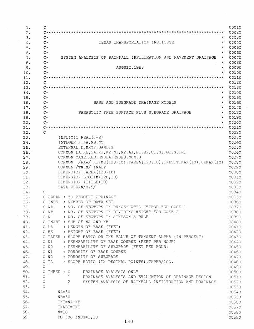
1. c 00010 2. C*****~*****~***********************************~*********************** 00020 3. 4.
6. 7. 8. 9.
10.
* 08030 TEXAS TRANSPORTATION INSTITUTE * 00040
* OOC5C * 00060
SYSTEH ANALYSIS OF RAINFALL INFILTRATION AND PAVEMENT DRAINAGE * 00070 * 00080
AUGUST,1983 * 00090 * 00100
11. C******************************************************************X**** 00110 12. c 00i20 13. C***********~*********~***~~************************x***********x***x*** 00130
14. 15. 16. 17. 18. 19. 20. 21. 22. 23. 24. 25. 26. 27. 28. 29. 30. 31. 32. 33. 34. 35. 36. 31. 38. 3:?. .:;.c. 41. 42. 43. 44. 45. 46. 47. 48. 49. 50. 51. 52. 53. 54. 55. 55. 57. 58. 59.
BASE AND SUBGRADE DRAINAGE MODELS
PARABJLIC FREE SURFACE PLUS SUBGRAJE DRAINAGE
* 00140 * 00150 * 00160 * 00170 * 00180 * 00190 * 00200
C***~*********************X********************************************~ 00210 00220 c
c c c c c ~
·~
,.., '--
c c c c c c c c c c c c c:
IKP~ICIT REAL(J-Z) ISTEGER N,NA,NB,NC: EXTERNAL DUMMYF,GAMDIS COMMON LA,HE,TA,K1,K2,Nl,N2,A1,B1,B2,Cl,Gl,G2,G3,R1 COMMON CASE,HED,HSUEA,ESUBB,NUM,S COHMON /RAW/ XTH:E (128, :8), YAREr~ (:20, 10), INDS, TIMA.X (10), UEM&'\: (10) COMMON /TNUM/ INABT DIMENSION UAREA(120,10) DIMENSION LOGTIM(120,10) DIMENSION ITITLE(18) IiATA IJDRAN/0. 5/
liD RAN 50 PERCENT JRAINAGE INDS NA KE N
NuMi3ER NO. OF NO. OF NO. OF
OF Dl'~TA SET SECTORS IN RUNGE-KUTTA METHOD FOR CASE ~
SECTORS IN DIVIDING HEIGHT FCR CASE 2 SECTORS !N SIMPSON'S RULE
INAB: SUH OF NA AND NB LA LENGTH OF BASE (FEET) HE HEIGHT OF BASE (FEE~)
TAPER SLOPE RATIO DR ~HE VALUE OF TANGENT ALPHA (IN PERCENT) PERMEABILITY OF EASE COURSE (FEET PER HOUR) PERMEABILITY OF SUBGRADE (FEET PER HOUR)
K1 K2 N1 POROSITY OF BASE COURSE N2 POROSITY OF SUBGRADE 'T"" _n SLOPE RATIO (IN DECIMAL POINTS) ,TAPER/10J.
I NEED 0 DRAINAGE ANAL~SIS ONLY 1 2
NA=30 NB=30 INT=NA-'-NB INABT=INT tJ=10
DRAINAGE ANALYSIS AND EVALUATION OF DRAINAGE DESIGN SYSTEM ANALYSIS OF RAINFALL INFILTRATION AND DRAINAGE
DO 300 INDS=1,l0 130
00230 00240 00250 00260 00270 00288 00290 00300 00310 00320 OC33C 00340 003.52• 00360 OG~70
00380 00390 004:)0 00410 00420 00430 004-4C 00450 00460 00470 00480 00490 00500 00510 00520 00530 00540 00550 00560 C057C 00580 00590

50. 61. 62. 63. 64. 65. 56. 57. 68. 69. 70. 71. 72. 73. 74. 75. 76. 77. 78. 79. so. Bl. 82. 83. 84. 85. 86. 87. 88. 89. 90. 91. a-o ~.:...
93. 94. 95. 96. 97. 98. 99.
100. l01. 102. 103. 104. 105. 106. 107. 108. 109. llO. lll. 112. 113. 114. 115. 116. 117. 118. 119.
c c
INPUT THE DATA
READ(5,55555,END=99999) IPROB,INEED,ITITLE 55555 FORMAT(I5,I3,18A4)
WRITE(6,55555) IPROB,ITITLE 55556 FORMAT(lH1,2(/),5X,'PROBLEM NUMBER',I5,2X,18A4)
IF(INEED.EQ.O) WRITE(6,55557) IF(INEED.EQ.1) WRITE(6,55558) IF(INEED.EQ.2) WRITE(6,55559)
55557 FORMAT(3(/) ,5X,'DRAINGE ANALYSIS USING TTI DRAINAGE MODEL') 55558 FORMAT(3(/),5X,'DRAINAGE ANALYSIS AND DESIGN EVALUATION') 55559 FORMAT(3(/) ,5X, 'SYSTEM ANALYSIS OF RAINFALL INFILTRATION AND DRAIN
AGE')
c c c
c c
c
c
IA=INDS READ(5,15)LA,HE,TAPER,K1,K2,N1,N2
15 FORMAT(7(F10.0)) TA=TAPER/100.
HORIZONTAL BASE COURSE
IF(TA.LE.O.) TA=0.1E-06 IF(N2.LE.O.) CALL POR02
IF N1 EQUALS TO N2 AND Kl EQUALS K2 WHICH IMPLIES BASE COURSE IS INFINITIVELY DEEP AND THE PROGRAM WILL NOT WORK
IF(Nl.EQ.N2.AND.K2.EQ.K1) K2=K2•1.000l WRITE(6,25)
25 FORMAT(3(/) ,5X, 'LENGTH' ,4X, 'BEIGHT' ,4X, 'SLOPE%', ~4X,'PERM.1',4X, 'PERM.2' ,4X, 'POR0.1' ,4X, 'POR0.2')
WRIT£(6,55)LA,HE,TAPER,Kl,K2,N1,N2 ~~ FORMAT(lX,3(F10.2l ,2(F10.5),2lFl0.4))
TWETA=LA•HE S=HE/ (LA•,T!~) WRITE(6,35)S
35 FCRMAT(//,5X, 'SLOPE FACTOR=' iF6.3//) WRITE(6,255)
255 FORMAT(5X, 'NOTE: THE FOLLOWING ANALYSIS IS BASED ON PARABOLIC SHAP +E PLUS SUBGRADE DRAINAGE')
00600 00610 00620 00630 00640 00650 00660 00670 00680 00690 00700 00710 00720 OCJ730 0074D 00750 00760 00770 00780 00790 00800 00810 00820 00830 00840 00850 00860 00870 00380 00890 00900 00910 00920 0093~
00940 00950 0Cl960
OJ970 00980 08990 ClOGO
C RUNGE-KUTTA METHOD FOR PARABOLIC(DQX) AND HORIZON~A~(DQY) EQUATION OF CAOlOlO c
WRITE(6,ll5) 115 FORMAT(6(/), 5X,'HEAD ON X COOR.' ,' HT. (SUB.DRAIN ONLY)'
1,8X,'AVG. HEIGHT.' ,7X,'TIME(STAGE 1) I ,7X,'DRAINAGE DEG.'//) TIME=O. XM=O. ll.K1=0. DELT=LA/NA CASE=l. DO 700 I2=1,NA TH!E2=TIME+AK1 XM=XM+DELT NUM=2. CALL SUBHT(TIME2,HSUB2) HSUBB=HSUB2 CALL CONS?C(XM,A) DTDX=DUMMYF{XM) AK2=DTDX•DELT
131
01020 01030 01040 01050 01060 01070 01030 01090 01100 OlllO
01120 Oll30 01140 01150 Oll60 Oll/0 01180 01190

120. 121. 122. 123. 124. l25. 126. 127. 128. 129. 130. 131. 132. 133. 134. 135. 136. 137. 138. 139. 140. 141. 142. 143. 144. 145. 146. 147. 148. 149. 150. 15l. 152. l-53. 154. l55. 156.
158. 159. 160. 161. 162. 163. 164. 165. 166. 167. 168. 169. 170. 171. 172. 173. 174. 175. 1'76. 177. 178. 179.
c
TIME=TIME+(AK1+AK2)/2. NUM=1. CALL SUBHT(T~ME,HSUB1) HSUBA=HSUB1 CALL CONSFC(XM,A) DTDX=DUMMYF(XM) AKl=DTDX*DELT WET1=(HE-HSUBA)*LA+HSUBA*XK/3. UE1=WET1/TWETA HAVG1=(TWETA-WE~l)/LA IF(HSUBA.LE.O.OR.HSUBA.LE.HAVG1) HSUBA=HAVGl WRITE(6,135)XM,HSUBA,HAVG1,TIME,UEl
135 FORMAT(5(E20.4)) XTIME(I2,IA)=TIM2 YAREA (I2, IA) =UE1
700 CONTINUE
C USE SIMPSON'S RULE IN CALCULATING TIME FOR CASE 2 C HSUBA(K!l .. XIMUM HEIGHT IN CASE 2) ,XM(TOTAL LENGTH IN CASE 1) C AND TIME(MAXIMUM TIME IN CASE 1) WERE ALL RESERVED FROM UPPER DO LOOP c
WRI'I'E(6,45) 45 FORMAT(lH1,6(/), SX, 'HEAD ON Y CCOR.' ,' HT. (SUB.DRAIN ONLY)',
800
300 59999
125
c
+8X,'AVG. HEIGHT' ,7X,'TIME(STAGE 2) I ,7X, 'DRAINAGE DEG.'//) CASE=2. HHAX=HSUBA HHAX2=HMAX DELTH=HMAX/NB DO 800 I3=1,NB
H:tUN=HMAX2-DE::...TH*::: 3 I5=I3+NA
IF ( I3. EQ. NB .OR. HM!N .LE. 0.) m:IN=HHAX*O. 5 CALL CONSFC(XM,HKIN) CALL SIMPS!; (A!:(E:..:'l .. , DUMr-!YF, HMIK, HMl0:, K)
TIHE=TIME+AREP. CALL SJBHT(TIME,HTSU) ~E'I'2=TWETA-2.*HMIN*LA/3. UE2=WET2/TWE':A HAVG2=(TWETA-WET2)/LA
IF(HTSU.LE.O.OR.HTSU.LE.HAVG2) E'I'SU=HAVG2 WRITE(6,135)HMIN,HTSU,HAVG2~'I'IME,U22
XTIME(I5,IA)=TIME YAREA(I5,IA)=UE2 UAREA(I5,IA)=YAREA(I5,~A)*l00.
HMAX=HMIN IF(I3.EQ.NB) TIMAX(IA)=TIME IF(I3.EQ.NB) UEMAX(IA)=UE2 CONTINUE H!AXD=TIMA.'{ ( IA) /24. +0. 5 CALL INPOLA(TDRAN,UDRAN,IA,LOGTIM) IF (I NEED. NE. 0)
1CALL JUDGE(IA,INT,ITYPFI,IQFINE,GRAVPC,SANDFC) IF(INEED.EQ.2) CALL RAIN(TDRAN,IMAXD) CONTINUE WRITE(6,125) FORMAT(lH1) STOP END
132
01200 G1210 01220 01230 01240 01250 01260 01270 01280 01290 01300 01310 01320 01330 01340 01350 01360 01370 01380 01390 01400 01410 01420 01430 01440 01450 01460 01470 014SO 01490 01500 01510 81520 01530 01340 OE::O Ol560 0:.:..570 o::..ssc 02.590 o:ssc 01610 01520 02_630 Ol640 01650 01660 Ol67C 01680 01690 01700 01710
01730 Cl740 01750 0::..760 01770 01780 01790

180. C*********************************************************************·** 01800 181. 182. 183. 184. 185. l86. 187. 188. 189. 190. 191. 192. 193. 194. 195. 196. 197. 198. 199. 200. 201. 202. 203. 204. 205. 206. 207. 208. 209. 2l0.
212. 213. 214. 2::..5. 216. 217. 218. 219.
221. 222. 223. 224. 225.
.226. 227. 228. 229. 230. 231. 232. 233. 234. 235. 236. 237. 238. 239.
C* * 01810 ,. 01820 ,. 01830 ,. 01840 * 01850 ,. 01860
C* VARIOUS CONSTANTS EMPLOYED IN EQUATIONS C* C* XM: lt,AXIMUM HORIZONTAL DISTANCE IN CASE 1; C* HiUN: MINIMU.I'I VALUE OF HEIGHT
C*********************************************************************** ,.... '-
c c
SUBROUTINE CONSFC(XM,HMIN) IMPLICIT REAL(J-Z) INTEGER N,NA,NB,NC,NJONT,NLANE COMMON LA,HE,TA,Kl,K2,N1,N2,A1,B1,B2,Cl,Gl,G2,G3,R1 COMMON CASE,HED,HSUBA,HSUBB,NUM,S IF(NUM.EQ.l.) HSUB=HSUBA IF(NUM.EQ.2.) HSUB=HSUBB
IF(CASE.EQ.2.) HSUB=HMIN IF(CASE.EQ.2.) XM=LA
Al=HSUB/SQRT(XH) Bl=A1*(1.-N1/N2) B2=Al*(K2/K1-Nl/N2) Cl=Nl*HE/N2 Gl=B1/B2 G2=C1 * ( l. -Gl) /E2 G3=C1*G2 R1=G3/B2 RETURN END
C***********************~**********~****************~******~****X*******
C* * C* CALCULATE DRAINAGE AREA CORRESPOND~NG TO DESIRED NUMBER OF DRY DAYS* C* YAREA,XTIME,':IMAX,UEHAX ARE THE SAHE AS PREVIOUSLY DSFIHED * C* IJRY : NUMBER OF DRY DAYS ; * c~ YDRAN: DRAINING AREA (IN %) COMPUTED BY INTRAPOLATION ; • C* *
01870 01880 01890 01900 01910 01920 01930 01940 01950 01960 01970 01980 01990 02000 02010 02020 02030 02040 02050 02060 02070 0208J 02090 02100 02110 02120 02130 02140 02150 02160
C********************~********************r*x**r.*************~********** 02170
C* C2l80 C* 02190
SUBROUTINE DRY:JAY (IMA.."I{D, YDRAN ,WP~CB) 02200 COMMON /RAW/ XTIME(l20,10},YAREA(120,10),INDS,TIMAX(l0) ,UEHAX(10) 02210 COMMON /TNUM/ INABT 02220 DIMENSION YDRAN(lOO),WPROB(50,50) 02230 IA=INDS 02240 DO 6000 I=1 I HlO 02250 IDRY=I 02260
DO 6100 I2=1,100 02270 IF(I2.EQ.INABT) GO TO 6222 02280 IF(XTIHE(I2,IA) .GT.IDRY*24.) GO TO Gll~ 02290
6100 CONTINUE 6111 Il=I2-1
IF(I1.LE.O) GO TO 6001 REGCOE=(YAREA(I2,IA)-YAREA(I1,IA))/(XTIME(I2,IA)-XTIME(Il,IA)) CONCOE=YAREA(I2,IA)-REGCOE*XTIME(I2,IA) YDRAN(IDRY)=(CONCOE+REGCOE*IDRY•24.)*100. GO TO 6000
6001 YDRAN(IDRY)=lOO.*YAREA(I2,IA)xiDRY*24./XTIME(I2,IA) 6000 CONTINUE 6222 IF(IMAXD.LE.O) RETURN
133
02300 02310 02320 02330 02340 02350 02368 02370 02380 02390

240. 241. 242. 243. 244. 245. 246. 247. 248. 249. 250. 251. 252. 253. 254. 255. 256. 257. ..,-p .... ~>.,.~.
259. 260. 261. 262. 263. 264. 265. 266. 267. 268.
270. 271. 272.
275. 275. 277. 278. 279. 280. 281. 282. 283. 284. 285. 286. 287. 288. 289. 290. 291. 292. 293. 294. 295. 296. 297. 298. 299.
H!AXD=IDRY IF(IM&XD.GE.39) IMAXD=39 YDRAN(IMAXD)=lOO. WRITE(6,6005)
6005 FORMAT(lHl,5(/) ,T34,'PROELEM NO.' ,5X,'T!ME(DAYS) ',4X,'DRAINAGE(%) I
2,2X,'PROE(CONSECUTIVE DRY DAYS) ',5t/))
02400 02410 02420 02430 02440 02450 02460 02470 02480 02490 02500 02510 02520 02530 02540 02550 02560 02570
IN=l D8 6600 I=l,IMAXD IN=IN+l WRITE(6,60lO)IA,I,YDRAN(I),WPROB(l,IN)
6010 FORMAT(T30,Il5,I15,F15.2,20X,F8.3,5(/)) 6600 CONTINUE
RETURN END
C***********************************************************************
C* C* ROUTINE F8R COMPUTING ALL THE FUNCTIONS C* C* X: MAXIMUM X VALUE FOR CASE l; X=LA FOR CASE 2;
MINIMUM X VALUE FOR CASE 3;
* * 02580 * 02590 * 02600 * 02610 * 02620
C**************************************~******************************** 02630 02640 02650 02660 02570 02680 02690 02700 0271.0 02720 02730 02740 02750 02750 02170 02780 02790 02800 02810 02820 C2830 02840 02850 02860 02870 02880 02890 02900 02910 02920 02930 02940 02950 02960 02970 02980
c c
FUNCTION rUMMYF(X) IMPLICIT REAL(J-Z) INTEGER N,NA,NE,NC,NJONT,NLANE COMMON LA,HE,TA,K1,K2,N1,N2,A1,El,B2,Cl,Gl,G2,G3,Rl COMM8N CASE,HED,HSUBA,HSUEB,NUM,S IF(NUM.EQ.l.) HSUB=HSUBA IF(NUM.EQ.2.) HSUB=HSUBB
IF(CASE.EQ.2.) AE=X IF(CASE.EQ.2.) X=LA IF(CASZ.EQ.2.) HSUB=AE
HED=HSUB IF(N2.GT.0.1E-05.AND.K2.NE.O.) GO TO 5555 DUM3=0. GO TO 6666
5555 FAC1=G1*X+2.*G2*SQRT(X)
c c
FAC2=2*Rl*ALOG(ABS((B2*SQRT(X)+C1)/Cl)) FACR=FAC1-FAC2 IF(N2.LE.0.1E-05) DQY=O. IF(N2.GT.O.lE-05)DQY=(HSUB*(l.-Nl/N2)+Cl)/(HSUB*(K2/K1-Nl/N2)+Cl) DUM3=6.*K2*X*((LA-X)*DQY+FACR)/LA
6666 CONTINUE IF(CASE.EQ.l.) DUM1=2.*Nl*HSUB*X IF(CASE.EQ.2.) DUM1=4.*N1*LA**2 DUM2=Kl*(3.*HSUB**2+4.*HSUB*X*TA) DUMMYF=DUM1/(DUM2+DUM3)
IF(CASE.EQ.2.) X=AE IF(CASE.EQ.2.) HSUB=HED
RETURN END
C*********************X***********************************************~*
C* * C* EVALUATE THE MODULI OF BASE AND SUBGRADE BY DISTRIBUTION * 02990
134

300. 301. 302. 303. 304. 305. 306. 307. 308. 309. 310. 311. 312. 313. 314. 315. 316. 317. 318. 3l9. 320. 321. 322. 323. 324. 325.-326. 327. 328. 329. 330. 331. 332. 333. 334. 335. 33E. 337. 338. 339. 340. 341. 342. 343. 344. 345. 346. 347. 348. 349. 350. 351.
353. 354. 355. -t:--'--b· 357. 358. 359.
C* OF MATERIAL SATURATION FROM THE RAINFALL C*
* 03000 * 03010 * 03020 * 03030 * 03040
C* ALPHA,BETA: PARAMETERS OF GAMMA DISTRIBUTION C* PWET,PDRY PROBABILITY OF WET AND DRY DAYS IN STEADY STATE C* HALFT ~IME OF 50% DRAINAGE(HOUR); C* C*
03050 03060
C******~**************************************************************** 03070 03080 03090
c c
c c c c c c c c .~ \...
c c c c c c
SUBROUTINE FLOWIN(ALPHA,BETA,PDRY,PWET,HALFT,CRKJON,IBC,ITYPE, 2ASOIL,BHORIZ,FTLONG,YEAR,AVGRAS,YDRAN,WPROB,IMAXD)
03100 03110 03120
GAMDIS: GAMMA DISTRIBUTION AS A FUNCTION 03130 AINTER,BSLOPE: INTERCEPT AND SLOPE OF THE LINEAR FUNCTION OF BASE COUR03140
MODULUS VS. WATER SATURATION DEGREE 03150 EMPDF : PROBABILITY DENSITY FUNCTION OF BASE COURSE MODULUS IN WET STA03160 PAVE INFILTRATION RATE OF PCC(1) OR BCP(2),UNIT=FT**3/(HOUR*FT) 03170 FLOAVG: I}iFILTRATION RATE SELECTED ACCORDING TO PAVEMENT TYPE 03180 PVA,PVB:THE INTERCEPT AND SLOPE OF REGRESSION EQUATION IN DEMPSEY'S TE03190 PX SPECIFIC RAINFALL AMOUNT 03200 CFHALF: THE AVERAGE DEGREE OF FREE WATER DRAINAGE PER HOUR 03210 DEFL DEFLECTION OF BASE MATERIALS (INCHES) 03220 DERATE: RATIO OF BASE MODULUS OF ELASTICITY 03230 BCMAT : EASE MODULI OF ELASTICITY (KSI) 03240 BCRATE: SLOPE OF DEFLECTION CHANGE WITH RESPECT TO DEGREE OF SATURATI003250 TURN?T: 1. DEFLECTION OF DRY BASE MATERIAL 03260
2. DEFLECTION OF 85% SATURATION LEVEL 03270 03280
REAL LA,K1,K2,N1,N2 03290 EXTERUAL GAl1DIS COMMON ~A,HE,TA,K1,K2,N1,N2,Al,B1,B2,C1,Gl,G2,G3,R1 COMMON CASE,HED,HSUBA,HSUBB,NU~,S COMMON /EDR/CONST,RECPOW,Dl!RPOW,SP.APE CQ}!MON /RAW/ XTIME(120,10) ,YAREA(120,1C) ,Hr:JS,T!::-IAX(10) ,UEHAX(lO) COMMON /TNUM/ INAET COMMON /SGwETl/ SGWET(100),SGDRY(l00) ,SGW(100),SG::J(lO:J) CO!-H>ION /NOGAMA/ lWHWET, AVGA.M'.:', TG'.:'St!!{
DIME~SION EMPDF(100),SGEM(100) ,AINTER(2,9),BSLO?E(2,9) DIMENSION PAVE(2),SOIL(9),HORIZ(2) ,PT!PE(2),FREE(100) DIMENSION PX(100),DURAT(100),SECT(20) ,CDF(20) ,IIA(lOO) DIMENSION DEFL(100) ,DERATE(100) ,BCRATE(2) ,BCMAT(6) ,TURNPT(2),
2BCEM(100) DIMENSION FREE2(100),DURATB(100) ,PXB(100) ,SECTB(50) DIMENSION YDRAN(100),WPROB(50,50) INTEGER PTYPE/'PCC' ,'BCP'/ DATA PAVE/0.03,0.11/ DATA PVA,PVB/0.32,0.48/ DATA BCMAT/425.3,236.3,209.3,64.6,29.8,17.1/ DATA BCRATE/0.24,3.5/,TURNPT/0.02,G.08/ REAL*B SOIL/'A-7-5' ,'A-4' ,'A-7-6' ,'A-6' ,'CL' ,'ML-CL',
2'CH' ,'ML' ,'MH'/,ASOIL INTEGER HORIZ/'ABC' ,'BC'/,BHCRIZ DATA AINTER/39.83,27.54,17.33,16.76,31.22,24.65,36.15,35.67,
2 31.89,32.13,31.89,32.13,21.93,23.02,31.39,29.01, 3 31.39,29.01/
DATA BSLOPE/0.453,0.266,0.158,0.146,0.294,0.196,0.362,0.354, 2 0.312,0.311,0.312,0.311,0.151,0.161,0.331,0.284, 3 0.331,0.284/
IF(IM~{D.GE.39) IM~Y.D=39
03300 03310 03320 03330 03340 03350 03360 03370 03380 03390 03400 03410 03420 03430 03440 03450 03460 03470 03480 03490 03500 03510 03520 03530 03540 03550 03560 03570 03580 03590

350. 361. 362. 363. 364. 365. 366. 367. 368. 369. 370. 371. 372. 373. 374. 375. 376.
378. 379. 380. 381. 382. 383. 354. 385. 386. 387. 388. 389. 390. """'0" .J~.L.
392 .. 393. 394. 395. 336. 397. 398. 399. 400. 401. 402. 403. 404. 405. 406. 407. 408. 409. 410. 411. 412. 413. 414. 415. 416. 417. 418. 419.
c
IF(ITYPE.EQ.PTYPE(1)) FLOAVG=PAVE(1} IF(ITYPE.EQ.PTYPE(2)) FLOAVG=PAVE(2} DO 7100 I=1,9
IF(ASOIL.NE.SOIL(I)) GO TO 7100 INDEXB=I GO TO 7555
7100 CONTINUE 7555 IF(BHORIZ.EQ.HORIZ(1)) INDEXA=1
IF(BHORIZ.EQ.HORIZ(2)) INDEXA=2
C FLOWMX: THE MAXIMUM AMOUNT WHICH WATER \>JOULD ENTER THE PAVEMENT C CC CARRYING CAPACITY OF WATER IN BASE COURSE (N1*L*H) c
c
CC=N1*LA*HE CFHALF=(0.5/HA~FT)*100.
C DISTRIBUTION OF PAVEMENT MODULI AND DRY, WET PROBABILITIES c
c c c
FREE DURAT I TEST
AMOUNT OF FREE WA:ER IN PAVEMENT(FEET**2) DURATION OF SPECIFIC RAINFALL AMOUNT(HOURS) l USING RIDGEWAY'S EQUATION; 2 USING DEMPSEY'S FOR NO CRACKS DATA AND WHEN RIDGEWAY'S METHOD TURNS OUT TO BE UNREASONABLE
IF(NUMWET-1)33333,22222,11111 11111 PX1=0.
c c c c c c
K=O CDFSUM=O. DO 7000 I=5,100,5 FREE(I)=CCxi*0.01
SGWET SGDRY SGH
\-lET DEPTH OF SUEGRADE DRY DEPTH OF SUBGRADE
SGD SGEN
FACTOR OF SUBGRADE MODULUS FOR WET ZONE (El**3) FACTOR OF SUBGRADE MODU:...US FOR DRY ZOUE SUBGRI>.DE MODU:.US
SGH (I)= (AINTER ( INDEXi"-., INDEX3) -BSLCPE ( INDEXA, INDEX3) *100.) 2 x(SGWET(I)**3)
IF(SGH(I) .LE.O.) SGW(I)=O. SGD (I) =A INTER ( INDEXA, INDE.XB) * (SGDRY (I)** 3) SGEM(I)=(SGW(I)+SGD(I))/((5.83333-HE)**3) IF(SGEM(I).LE.O.) SGEM(I)=O. IF(CRKJON.EQ.O.) GO TO 7777 ITEST=1 DURAT(I)=(FREE(I)*FTLONG)/(CRKJCN*FLOAVG) PX(I)=(60.*DURAT(I))**(1.-DURPOW)*CONST*(YEARx*RECPOW)/SHAPE RIDGE=BETA*PX (I) IF(RIDGE.GE.174.) GO TO 7777 GO TO 7788
7777 ITEST=2 PX(I)=((FREE(I)*FTLONG*0.02832-PVA)/(PVB*0.02832*FTLONG*LA))*12. IF(PX(I) .LE.O.) PX(I)=O. DURAT(I)=((PX(I)*SHA?E)/(CONST*(YEAR**RECPOW)))**(1./(l.-DURPOW))
2 /60. 7788 PX2=PX(I)
EMPDF(I)=GAMDIS(PX2,ALFHA,BETA) IF(I.GT.85) GO TO 7755 IF(I.LE.60) GO TO 7744
DEFL(I)=TURNPT(1)+BCRATE(1)*C.01*(I-60) DERATE(I)=TURNPT(1)/DEFL(I)
136
03600 03610 03620 03630 03640 03650 03660 03670 03680 03690 03700 03710 03720 03730 03740 03750 03760 03770 03780 03790 03800 03810 03820 03830 03840 03850 03860 03870 03880 03890 03900 03910 0392::-: 03930 03940 03950 03960 03970 03980 03990 04000 04010 04020 04030 04040 C4050
. 04060 04070 04080 04090 04100 04110 04120 04130 04140 04150 04160 04170 04180 04190

420. 42l. 422. 4Z3. 424. 425. 426. 427. 428. 429. 430. 431. 432. 433. 434. 435. 436. 437. 438. 439. 440. ~41.
442. 443. 444. 445. 446. 447. 448. 449. 450.
c c c c
c
c c c c
BCEM(I)=BCMAT(IBC)*DERATE(I) GO TO 7766
7744 BCEM(I)=BCMAT(IBC) DERATE (I) =1. 0 GO TO 7766
7755 DEFL(I)=TURNPT(2)+BCRATE(2)*0.0l*(I-85) DERATE(I)=TURNPT(1)/8EFL(I)
BCEM(I)=BCMAT(IBC)*DERATE(I) 7766 IIB=I/10*10
IF(IIB.NE.I) GO TO 7000 CALL SIMP2(SECTOR,GAMDIS,PXl,PX2,60,ALPHA,BETA) K=K+1 IF(SECTOR.LE.O.) SECTOR=O. IF(SECTOR.GT.1.0) SECTOR=1.0 SECT(K)=SECTOR CDFSUM=CDFSUM+SE:T(K) IF(CDFSUM.GE.1.0) CDFSUM=l.O CDF(K)=CDFSUM PX1=PX2
7000 CONTINUE
04200 04210 04220 04230 04240 04250 04260 04270 04280 04290 04300 04310 04320 04330 0434C 04350 04360 04370 04380 04390 04400
CALCULATE THE PART WHICH IS BEYOND THE FIELD CAPACITY IN GAMMA DISTRIB0441C ?X2 IS THE HAXI!-!UM INFILTRATION AMOUNT AFTER THE ABOVE LOOP 04420
TAILPT=1.0-CDFSUM
THE DRY AND WET PAOBABILITIES OF THE PAVEMENT
PAVDRY: THE DRY PROBABILITY OF PAVEMENT ?AVWET: THE WET PROBABILITY OF PAVEMENT
04430 04440 04450 04460 044'70 04430 04490 04500
451. IF(TIMAX(INDS)/24.LT.1.) GO TO 8833 04510 452. PX.l=O. 0452rJ 453. K=O o.:;~30
454. DO 8000 I=l, IM.1l.XD 04540 455. :?REE2 (I) =CC'' G. Oi * Y:SRAN (I) o.;s:;c; 455. IF(CRKJON.EQ.O.) GO TO 8777 04560 457. !TEST=: CJ457C! 458. DU2ATB(I)=(FREE2(I)•FTLONG)/(CRK20N*F~OAVG) o.;ssc 459. PXB(I)=(60.*DURATB(I))••(!.-JURPOW)•CO~ST*(YEAR••RECPOW)/SEAPE G45SO 460. RIDGE=BE~A*PXB(I) 0~600
46~. IF(RIDGE.GE.174.) GO TO 8777 046l0 462. GO TO 8788 04620 463. 8777 ~TEST=2 04630 454. PXB(I)=((FREE2(I)*FTLONG•0.02832-PVA)/(PVB*0.02832•FTLONG•LA))*12. 04640 465. IF(PXB(I) .LE.O.) PXB(I)=O. 0">550 466. DURATB(I)=((PXB(I)•SHAPE)/(CONST*(YEAR•*RECPOW))) 04660 467. 2*•(1./(l.-DURPOW))/60. 04570 468. 8788 PX2=PX3 (I) C468::J 469. CALL SIMP2(SECTOR,GAMDIS,PXl,PX2,60,ALPHA,BE~A) 04690 470. K=K+1 0~700
471. IF(SECTOR.LE.O.) SECTOR=O. 04710 472. IF(SECTOR.GT.l.O) SECTOR=1.0 04720 473. SECTB(K)=SECTOR 04730 474. PXl=PX2 04740 475. 8000 CONTINUE 04750 476. PAVDRY=O. o.;150 477. IN=1 0477C 478. DO 8100 K=l,IHAXD 04780 479. IN=IN~l 04'790
137

480. 481. 482. 483. 484. 485. 486. 487. 488. 489. 490. 491. 492. 493. 494. 495. 496. 497. 498. ~99.
500. 501. 502. 503. 504. 505. 506.
508. 509. 510.
PAVDRY=PAVDRY+SECTB(K)•WPROB(1,IN) 8100 CONTINUE
PAVDRY=PAVDRY+WPROB(1,IN)•TA~LPT
GO TO 8844 8833 DHALF=HALFT/24.
PAVDRY=1.-PWET•DHALF 8844 PAVWET=1.-PAVDRY
c c C CALCU~ATE THE PROBABILITIES OF SATURATION LEVELS: C SECT1: 0-60%; SECT2: 60-85%; SECT3: 85-100% c c
c
CALL SIM?2(SECT1,GAMDIS,O.,PX(60) ,60,ALPHA,BETA) IF(SECT1.GE.1.0) SECT1=1.0 CALL SIMP2(SECT2,GAMDIS,PX(60) ,PX(85),60,ALPHA,EETA) CALL SIMP2(SECT3,GAKDIS,PX(85) ,PX(100),60,ALPHA,BETA) SECT3=SECT3+TAILPT
GO TO 44444 C NUMBER OF RAINFALL QUANT~TY EQUALS TO 0 OR 1 (NO GAMMA DISTRIBUTION) c C YRAINl: DRAINAGE LEVEL OF ONE RAINY DAY (IN DECIMAL POINT) C TRAIN1: T:ME FOR THE CORRESPOND~NG DRAINAGE LEVEL OF ONE RAINY DAY
22222 ITEST=1 IF(CRKJON.EQ.O.) GO TO 9191 AVGDUR=(AVGRAS•0.08333•LA•FTLONG)/(CRKJON•FLOAVG) AVGFL0=(60.•AVGDUR)••(1.-DURPCW)•CONST•(YEAR••RECPOW)/SHAPE G8 T8 9292
9191 ITEST=2
04800 04810 04820 04830 04840 04850 04860 04870 04880 04890 04900 04910 04920 04930 04940 04950 04960 04970 04980 04990 05000 05010 05020 05030 05040 05050 05060 05070 05080 05090 8-5100
511. AVGDUR=(SHAPE•AVGRAS/(CONST•(YEAR••RECP:JW)))••(l./(1.-DURPOW))/60. 05110 512. AVGFLO=(PVB•AVGRAS•0.08333•?TLONG•LA•0.02832+PVA)/(0.02832•FTLONG) 0512J 5:3. 9292 ~RAIN:=AVGFLO/CC 05130 514. c 05140 !:15. 516. 517.
519. 520. 521. 522. 523. 524. 525. 526. 527. 528. 529. 530. 531. 532. 533. 534. 535. 536. 53'7. 538. 539.
C FIND THE CORaESPONDING TIME FOR DEGREE OF DRAINAGE
20 9900 I2=2,l00 IF(I2.EQ.INABT) GO TC 9922 IF(YAREA(I2,INDS).GE.YRAINl) GO TO 9911
99CO CCUT~NTIE
9911 Il=I2-1 REGCOE=(XTIME(I2,INDS)-XTIME(I1,INDS))/
2 (YAREA(I2,INDS)-YAREA(I1,INDS)) CONCOE=XTIME(I2,INDS)-REGCOE•YAREA(I2,INDS) TRAIN1=CONCOE+REGCOE•YRAINl GO TO 9933
9922 TRAIN1=TIHAX(INDS) 9933 PAVWET=TRAIN1/(TOTSuM•24.)
PAVDRY=1.-PAVWET IF(YRAINl-0.85) 9944,9944,9955
9944 SECT3=0. GO TO 9966
9955 SECT3=XTIME(103,INDS)/TOTSUM 9966 IF(YRAIN1-60.)9988,9988,9977 9977 SECT2=(XTIME(108,INDS)-XTIME(103,INDS))/TOTSUM
GO TO 9999 9988 SECT2=0. 9999 SECT1=1.-SECT2-SECT3
44444 DEFL(73)=TURNPT(1)+BCRATE(l)•O.l25
05150 OSlSO 05170 05180 05190 052CO 05210 05220 05230 05240 05250 05260 05270 05280 05290 05300 05310 05320 05330 05340 0535:J 05360 05370 05380 05390

540. 541. 542. 543. 544. 545. 546. 547. 548. 549. 550. 551. 552. 553. 554. 555. 556. 551. 558. 559. 560. 561. 562. 563. 564. 565. 566. 567. 568. 569. 570.
572. 573. 574. 575. 576. 5'77.
578. 579. 580. 581. 582. 563. 584. 585. 586. 587. 588. 589. 590. 591. 592. 593. 594. 595. 596. 597. 598. 599.
c c c c c c c c c
c c c
DERATE(73)=TURNPT(l)/DEFL(73) DEFL(93)=TURNPT(2)+BCRATE(2)•0.075 DERATE(93)=TURNPT(l)/DEFL(93) AVBCEM=BCMAT(IBC)•(l.•SECTl+DERATE(73)•SECT2+DERATE(93)•SECT3) GEBCEM=AVBCEM•PAVWET+BCMAT(IBC)•PAVDRY
AVERAGE RAINFALL DURATION AND BASE COURSE MODULUS
AVGDUR: DURATION CORRESPONDING TO THE AVERAGE RAINFALL AMOUNT AVGFLO: FREE WATER IN PAVE.HENT DUE TO AVERAGE RAINFALL AMOUNT GESGEM: TOTAL AVERAGE OF SUBGRADE MODULI AVECEM: AVERAGE BASE MODULI IN WET STATE GEBCEM: TOTAL AVERAGE OF EASE MODULI
AVGDUR=(SHAPE•AVGRAS/(CONST*(YEAR••RECPOW)))••(1./(1.-DURPOW))/60. IF(ITEST.EQ.2) GO TO 8888 AVGFLO=FLOAVG•AVGDUR•CRKJON/FTLONG GO TO 8899
8888 AVGFLO=(PVB•AVGRAS•0.08333•FTLONG•LA*0.02832+PVA)/(0.02832*FTLONG) 8899 IF(AVGFLO.GE.CC) AVGFLO=CC
CALCULATE SUBGRADE MODULI
EXACT2=AVGFLO/CC DO 9100 I2=l,l00
IF(EXACT2.GE.l.) GO TO 9222 IF(YAREA(I2,INDS) .GT.EXACT2) GO TO 9111
9100 CONTINUE 9111 Il=I2-l
IF(I1.LE.O) GO TO 9001 PEGCOE=(XTIME(I2,INDS)-XTIME(Il,INDS))/
2 (YAREA(I2,INDS)-YAREA(I1,INDS)) INCEPT=XTIME(I2,INDS)-REGCOE~YAREA(I2,INSS)
TSGAVW=INCEPT+REGCOE*EXACT2 GO TO 9333
9001 TSGAVW=XTIME(l,!NDS)•EXACT2/YAREA(1,INDS) GO TO 9333
9222 TS::.AVW=T:HAX(INDS) 9333 CAL~ SUBHT(TSGAVW,HSUBEM)
c C SGWETD: AVERAGE 'i-!E':' DSPTH OF SU33RADE DURING THE SEASON C SGDRYD: AVERAGE DRY DEPTH OF SUEGRADE C SGl FACTOR OF SUBGRADE MODULUS FOR WET ZONE (El**3) C SG2 FACTOR OF SUBGRADE MODULUS FOR DRY ZONE c
c
SGWETD=(HE-HSUBEM)*Nl/N2 IF(S3WETD.LE.O.OR.K2.EQ.O.) SGWETD=O. SGDRYD=5.83333-HE-SGWETD SGl=(AINTER(INDEXA,!NDEXB)-3SLOPE(INDEXA,INDEXB)•lOO.)*(SGWETD•*3) IF(SGl.LE.O.) SG1=0. SG2=AINTER(INDEXA,INDEXB)•(SGDRYD**3) GESGEM=(SG1+SG2)/((5.83333-HE)•*3)
IF(NUMWET.LE.1) GO TO 55555 WRITE(5,735)CC,CFHALF,TAILPT,PAVDRY,PAVWET
735 FCRMAT(3(/),T40, 'WATER CARRYING CAPACITY OF BASE(SQ.FT)=' ,Fl0.3,/, 2 3 4 5
T40,'AVERAGE DEGREE OF DRAINAGE PER HOUR =' ,Fl0.3,/, T40,'0VERALL PROBABILITYT OF SATURATED BASE=' ,F10.3,/,
//,T40,'DRY PROBABILITY OF BASE COURSE =',Fl0.3,/, T40,'WET PROBABILITY OF BASE COURSE =' ,Fl0.3)
05400 05410 05420 05430 05440 05450 05460 05470 05480 05490 05500 05510 05520 05530 05540 05550 05560 05570 05580 05590 05600 05610 05620 05630 05640 05650 05660 05670 05630 05690 05700 05710 05720 'J5730 05740 C5750 05760 05770 05780 05790 05300 05310 05820 05830 05840 05850 05860 05870 05880 05890 05900 05910 05920 05930 05940 05950 05960 05970 05980 05990

600. 601. 602. 603. 604. 605. 606. 607. 608. 609. 610. 611. 612. 613. 614. 615. 616. 617. 618. 619. 620. 621. 622. 623. 624. 625. 626. 627. 528.
630. 531. 632. 633. 634. 535. 636. 637. 638. 539. 640. 641. 642. 643. 644. 645. 646. 647. 648. 649. 650. 551. 652. 653. 554. 655. 656. 657. 658. 659.
c
IF(ITEST.EQ.2) WRI~E(6,745)
745 FORMAT(//,T30,' (THE ANALYSIS FOR WATER ENTERING PAVEMENT IS BASED 20N DEMPSEY¢S FIELD EQUATION)')
IF(ITEST.EQ.1) WRITE(6,755) 755 FORMAT(//,T30,'(THE ANALYSIS FOR \>TATER EN~ERING PAVEMENT IS BASED
20N RIDGEWAY¢S LAB EQUATION)') WRITE(6,705)
705 FORMAT(//,T35,'**********PROBABILITY DISTRIBUTION OF MODULUS 0~ BA 2SE COURSE**********',///)
7200
2 3 4 5
DO 7200 I=1,10 IIA(I)=I*10 WRITE(6,715) (IIA(I) ,I=1,10), (FREE(I) ,I=l0,100,10),
(PX(I) ,I=l0,100,10), (DURAT(I) ,I=10,100,10), (BCEM(I),I=lO,lOO,lO),(DERATE(I),I=10,100,10), (SGEM(I), I=10,100,10), (EMPDF(I), I=10,100,10), (SECT(K),K=1,10),(CDF(K),K=1,10)
'715 1 2
FORMAT(~25,'SATURATION LEVEL (%)' ,10I7,//, T25,'WATER IN BASE(SQ.FT) I ,10F7.2,//, T25,'RAINFALL QT.(INCHES) I ,10F7.2,//, T25,'RAIN DURATION(HOURS)' ,10F7.2,//, T25,'BASE MODULI (KSI) I ,10F7.2,//, T25,'RATIO OF DRY MODULUS' ,10F7.2,//, T25,'SUBGRADE MODULI(KSI) ',10F7.2,//, T25,'PROBABILITY DENSITY' ,10F7.2,//, T25,' PROBABILITY' ,10F7.2,//,
3 4 5 6 7
8 9 T25,'CUMULA~IVE PROB.' ,lOF7.2)
WRITE(6,775)AVGFLO,AVGDUR,AVGRAS,AVBCEM,GEBCEM,GESGEM 775 FORMAT(//,T40,'***** DISTRIBUTION CHARACTERISTICS OF RAIN?ALL EFFE
2C': *****', 3//,T30,'AVERAGE FREE WATER IN BASE (SQ.FEET)=' ,Fl0.2, 4/ I I T30 I I DURATION OF AVERAGE RAINFALL ll.M·JUNT (HOURS)= I , FlO. 3 I
5// 1 T30,'AVERAGE RAINFALL AMOUNT PER DAY (INCHES)=' ,Fl0.3, 6//,T30 1 'AVERAGE BASE COURSE KO~ULUS IN WET STA~E(KSI)=' ,Fl0.2, 7// 1 T30,'AVERAGE BASE COURSE MODULUS (KS!)=',F10.2, 8//,~30, 'AVERAGE SU3GRADE f!ODULUS (KS!)=' ,:'10.2)
R£TURN
C A SEASON IS COMPLETE DRY c 33333 PAVDRY=l.
PAVWET=O. AVGRAS=O. AVGDUR=O. AVGFLO=O. AVBCEM=BCMAT(IBC) GEBCEM=AVBCEM AVSGE:H=AINTER (INDEXA, INDEXB) GESGEM=AINTER(INDEXA,INDEXB)
C PRINTOUT FOR ONLY ONE RAINY DAY OR A COMPLETE DRY SEASON c 55555 WRITE(6,785)
785 FORMAT(3(/) ,T40,'***************************************' ,/, 2 //,T10,'NO GAMMA DISTRIBUTION IS APPLIED TO THIS ANALYSI 3S DUE TO ONLY ONE OR NO RAINFALL QUANTITY IS FOUND',//)
IF(ITEST.EQ.2) WRITE(6,745) IF(ITEST.EQ.l) \>TRITE(6,755) WRITE(6,765)PAVDRY 1 PAVWET,
2 AVGFLO,AVGDUR,AVGRAS,AVBCEM 1 C2BCEM,GESGEM 765 FORMAT(
140
06000 06010 06020 06030 06040 06050 06060 06070 06080 06090 06100 06110 06120 06130 06140 06150 06160 06170 06180 06190 06200 06210 06220 06230 06240 06250 06260 06270 06280 06290 06300 06310 0632C 06330 06:340 06350 06360 05370 06380 06390 06400 06410 06420 06430 06440 06450 06460 06470 06480 06490 06500 06510 06520 06530 06540 06550 06560 06570 06580 06590

660. 661. 662. 663. 664. 665. 666. 667. 668. 669. 670. 671. 672. 673. 674.
676. 677. 678. 679. 680. 681. 682. 683. 684. 685. 686. 68'7. 688. 589. 690. 691.
693. 594. 695. 696. 697. 698. 699. 700.
702. 703. 704. 705. 706. 707. 708. 7:)9. 710. 711. 712. 713. 714. 715. 716. 717. 718. 719.
c c
2//,T30,'DRY PROBABILITY OF BASE COURSE 3//,T30,'WET PROBABILITY OF BASE COURSE 4//,T30,'AVERAGE FREE WATER IN BASE 5//,T30,'DURATION OF AVERAGE RAINFALL AMOUNT 6//,T30,'AVERAGE RAINFALL AMOUNT PER DAY 7//,T30,'AVERAGE BASE COURSE MODULUS IN WET 8//,T30,'AVERAGE BASE COURSE M8DULUS 9//,T30,'AVERAGE SUBGRADE MODULUS
RETURN END
=' , FlO. 3, =',FlO. 3,
(SQ.FEET)=' ,Fl0.2, (HOURS)=' ,Fl0.3,
(INCHES)=' ,Fl0.3, STATE(KSI)=' ,Fl0.2,
( KS I ) = ' , F 1 0 • 2 , ( KS I ) = ' , F 1 0 • 2 )
C*******************X*************************************************~*
C* *
06600 06610 06620 06630 06640 06650 06660 06670 06680 06690 06700 06710 06720 06730
C* COMPUTING PROBABILITIES OF CONSECUTIVE DRY DAYS BY KATZ'S METHOD C*
* 06740
* C*****************************************************************x*****
c c
c c c c c c
c
c c c
c
c
SUBROUTINE KATZ(IM&XD,W) DIMENSION WZER0(50,50) ,WONE(50,50) ,W(50,50) COI-!MON /DRYW:t:T / TLAMDA, DRY LAM, WET LAM, PWET
KATZ'S METHOD TO COMPUTE THE DISTRIBUTION OF WET AND DRY DAYS IN CERTAIN PERIOD, WHICH IS ASSOCIATED WITH MARKOV CHAIN MODEL WZERO(I,J): THE PROBABILITY OF I-10 WET DAYS IN J CONSECUTIVE DAYS
WHEN THE ZEROTH DAY IS DRY WONE (I,J): THE PROBABILITY OF I-10 WET DAYS IN J CONSECUTIVE DAYS
WHEN THE ZEROTH DAY IS WET MAX\.JET: TIME REQUIRED TO DRA:J:N OUT 99~;; HATER Il{ THE PAVEMENT
IF(TLAMDA.GE.l74.) EXPCON=O. IF (TLAMDA. LT .l 74.) EXPCON=EXP ( -TLA?-WA) POO= (WETLAM+DRYLF>.H*EXPCON) /TLAHDA POl=DRYLM!* (1. -:t:XPCONj /TLAHDA PlO=WETLAMx(l.-EXPCON)/TLAMDA Pll=(DRYLAM~WETLAM~EXPCOH)/TLAMDA
WRITE(6,45) POO,P01,PlO,Pll 45 FORMAT(5(/) ,T30, '********** TRA!'l"SI'IIQN PROBABIL..ITY l!ATRIX **"***"*
2**' ,3(/) ,T40, 'POO=' ,F5.3,10X, 'PO:l.=' ,F5.3,//, 3 T40,'P10=',F5.3,10X,'P11=' ,F5.3)
\>!ZERO ( 10, 11) =POO WZER0(11,1l)=POl WONE(10,11)=P10 WONE (11, 11) =Pll WZERO (10, 10) =l. WCNE(10,10)=l.
IF ( IMAXD. GE. 39) IMAXD=39 MXWTP1=IMAXD+l DO 200 NJ=2,MXWTP1 DO 100 K=1,NJ
NJ10=NJ+10 K10=K+10 NJ9=NJ10-1 NJ8=NJ9-1 K9=Kl0-l K8=K9-1
WONE(-1;N-1)=Q. WONE(9,NJ8)=0.
WZERO(N;N-1)=0. WZERO(NJ9,NJS)=O.
1 41
06750 06760 06770 06780 06790 06800 06810 06820 06830 06840 06850 06860 06870 Ot:880 06890 06900 06910 06920 OE930 06940 06950 05960 06970 06980 06990 07000 07010 07020 07030 07040 07050 07060 C7070 07C80 07090 07100 07110 07120 07130 07140 07150 07150 07170 07180 07190

720. 721. 722. 723. 724. 725. 726. 727. 728. 729. 730. 731. 732. 733. 734. 735. 736.
738. 739. 740. 741. 742. 743. 744. 745. 746. 747. 748. 749 .. 750. 751. 752. 753. 754. 755. "56.
7-~ ,::Jo.
759. 761J. 761. 762. 763. 754. 765. 766. 767. 768. 769. 770. 771. 772. 773. 774. 775. 776. 777. 778. 779.
c c c c c c
c c c c c c c c c c
c c
WZERO(K9,NJ9)=POO*WZERO(K9,NJ8)+P01*WONE(K8,NJ8) WONE(K9,NJ9)=PlO*WZERO(K9,NJ8)+P11*WONE(K8,NJ8) W(K9,NJ9)=(1.-PWET)*WZERO(K9,NJ9)+PWET*WONE(K9,NJ9)
100 CONTINUE 200 CONTINUE
CONVERT THE I+lO SEQUENCE TO LOWER SERIES STARTING FROM , WHICH STANDS FOR DRY DAY, 2 FOR 1 WET DAY ....•..
DO 500 I=l,MXWTPl DO 500 J=1,I
I10=I+9 J10=J+9 WONE(J,I)=WONE(JlO,I10) WZERO(J,I)=WZERO(J10,Il0) IF(I.GT.l)W(J,I)=W(JlO,IlO)
500 CONTINUE
WRITE(6,:35) 35 FORMAT(lHl,5X, 1 ********** PROBABILITIES OF K WET DAYS IN COSECUTIV
2E N DAYS ********** 1 ,5(/) ,T40,45( 1 - 1 ) ,//,T40,4X, 1 N1 ,4X, 1 K 1 ,
+3X, 1 '\\'0(K;N) I ,3Z, 1 Wl(}:;N) I ,4X, 'W(K;N) I)
DC 400 J2=l,I.HAXD J3=,T2+l
WRITE(6,25) FORMAT(//,T40,45( 1 - 1 ) ,//)
DO 300 I2=l,J3 J210=J2+l I29=I2
C Il=I2-l C WRITE(6,l5)J:,Il,WZERO(I29,JZlC) ,WONE(I23,J2l0), C 2 W(I29,J2lO) C 15 FOR.HAT(T40,I5,I5,3Fl0.3) C 300 CONTI!;-TJE
07200 07210 07220 07230 07240 07250 07260 07270 07280 07290 07300 07310 07320 07330 07340 07350 07360 07370 07380 07390 ('7400 07410 07420 07430 07440 07450 07460 07470 07480 07490 07500 07510 07520 07530 07540 0755·0 ~7560
C 400 CONTINUE 07570 RETURN 07580 END 07590
c 07600 c 07610 C*******************************************~~*************************** 07620
C* CALCULATE THE DESIRED DRAINING AREA EY INTRAPOLATION C*
* 07630 * 07640
C* XTIME: TIKE ( X COORDINATE ) ; C* YAREA: DRAINING AREA ( Y COORDINATE C* TDRAN: TIME OF 50 PERCENT DRAINAGE; C* UDRAN: 50 PERCENT DRAINAGE; C* TIM~Y-: M&XIMU.H VALUE FOR TIME; C* UEMAX: MAXIMUM v;,LUE FOR DRAINAGE; C*
* * * * * * * *
C******************************************************************~****
SUBROUTINE INPOLA(TDRAN,UDRAN,IA,LOGTI~) IMPLICIT REAL(J-Z) COMMON /RAW/ XTIME(l20,10) ,YAREA(l20,10) ,INDS,TI.H&X(10) ,UEM~2(:o) COMMON /TNUM/ INABT COMMON LA,HE,TA,Kl,K2,H1,N2,Al,B1,B2,Cl,Gl,G2,G3,Rl
142
07650 07660 07670 07680 07690 07700 C77l0 07720 07730 07740 07750 07760 07770 07780 07790

780. 781. 782. 783. 784. 785. 786. 787. 788. 789. 790. 791. 792. 793. 794. 795. 796. 797. 798. 799. BOO. 801. 802. 803. 804. 805. 806. 807. 808. 809. 810. 811. 812. 813. 81.;,. 815. 816. 817. 818. 819. 820. 821. 822. 823. 824. 825. 826.
.827. 828. 829. 830. 831. 832. 833. 834. 835. 836. 837. 838. 839.
c c c c c c
COMMON CASE,HED,HSUBA,HSUBB,NUM,S COMMON /SGWET1/ SGWET(100) ,SGDRY(100),SGW(100) ,SGD(100) DIMENSION LOGTIM(120,10) ,YAPER(120,10) DATA IPT/20/ REAL INCEPT
SGEMT SGWET SGDRY SGDEP
TOTAL SUBGRADE MODULUS WET DEPTH OF SUBGRADE DRY DEPTH OF SUBGRADE DEPTH OF SUBGRADE (TOTAL DEPTH OF BASE AND SUBGRADE IS 70IN)
IA=INDS DO 1000 I=1,IPT EXACT=l. 0* I/IPT
IX=100*I/IPT SGDEP=5.83333-HE
DO 1100 I2=1,100 IF(I2.EQ.INABT) GO TO 2222 IF(YAREA(I2,IA).GT.EXACT) GO TO 1l1l
1100 CONTINUE 1111 Il=I2-l
IF(I1.LE.O) GO TO 1001 REGCOE=(X~IME(I2,IA)-XTIME(I1,IA))/(YAREA(I2,IA)-YAREA(I1,IA)) INCEPT=XTHIE(I2,IA)-REGCOE*YAREA(I2,IA) IlOO=I+100 XTIME(I100,IA)=INCEPT+REGCOE*EXACT YAREA(I100,IA)=EXACT
CALL SUBHT(XTIME(I100,IA),HSUBX) SGWET(IX)=(HE-HSUBX)*N1/N2 IF(SGWET(IX).GE.SGDEP) SGWET(IX)=SGDEP IF'(SGWET(IX) .LE.O.OR.K2.EQ.O.) SGWET(IX)=O. SGDRY(IX)=5.83333-HE-SGWET(IX)
IF (IE' IX ( 100*EXACT) . EQ. !FIX ( lOO*UDRJ..N)) TDRAN=XTIME ( IlOO, IA) GO TO 1000
1001 IlOO=I+100 XTIME(I100,IA)=XTIME(I2,IA)*EXACT/YAREA(I2,IA) YAREA(IlOO,IA)=EXACT CALL SUBHT(XTIME(I100,IA},HSUBX) SGWET(IX)=(HE-HSUBX)*N1/N2 IF(SGVlET(IX) .GE.SGDEP) SGWET(IX)=SGDEP IF (SGWET (IX) .LE.O .OR.K2. EQ. 0.) SG'iolET (IX) =0. SGDRY(IX)=5.83333-HE-SGWET(IX)
1000 CONTINUE 2222 IMAX=Il00+1
XTIME(IMAX,IA)=TIMAX(IA) YAREA(IMAX,IA)=UEMAX(IA) CALL SUBHT(XTIME(IMAX,IA),HSUBX) SGWET(IX)=(HE-HSUBX)*N1/N2 IF(SGWET(IX) .GE.SGDEP) SGWET(IX)=SGDEP IF(SGWET(IX).LE.O.OR.K2.EQ.O.) SGWET(IX)=O. SGDRY(IX)=5.83333-HE-SGWET(IX) WRITE(6,2)
2 FORMAT(1H1,5(/) ,T30,'DRAINAGE%',11X,'TIME' ,5X,'PROBLEM NO.') DO 1200 I7=101,IMAX
YAPER(I7,IA)=YAREA(I7,IA)*100. 1200 CONTINUE
305
DO 1600 IB=1,20 IB100=I3+100 WRITE(6,305)YAPER(IB100,IA) ,XTIME(IB100,IA),IA FORHAT(T30,F9.1,5X,E10.3,Il5)
143
07800 07810 07820 07830 07840 07850 07860 07870 07880 07890 07900 07910 07920 07930 07940 07950 07960 07970 07980 07990 08000 08010 08020 08030 08040 08050 08060 08070 08080 08090 08100 08110 08120 08l3C 08140 08::.50 08160 09::.70 08180 08190 08200 08210 08220 08230 08240 08250 08260 08270 08280 08290 08300 08310 08320 08330 08340 08350 08360 08370 08380 08390

840. 841. 842. 843. c
1600 CONTINUE RETURN END
08400 C841:J 08420 08430
844. c 08440 645. C***********************************************X~********************** 0845G 846. 847. 848. 843. 850. 851. 852. 853. 854. 855. 856. 857. 858. 859. 850. 861. 662. 86:3. 864. 865. 866. 867. 868.
870. 87l. 372. 873. 574. 875. 876. e77. 878. 879. 880. 881. 882. 883. 884. 885. 885. 887. 888. 889. 890. 891. 892. 893. 894. 895. 896. 897. 898. 899.
C* EVALUATION OF THE DRAINAGE DESIGN FOR GRANULAR LAYERS C* C* 85% SATURATION C* SATISFACTORY: LESS THAN 5 HOURS C* MARGINAL 5 TO 10 HOURS C* UNACCEPTABLE: GREATER THAN 10 HOURS C* C* PERIND: PERCENTAGE INDEX, THE PERCENTAGES OF WATER C* CAN BE DRAINED IN A SATURfi.TED SM:PLE ... C* IQFINE: CATEGORY OF FINES AMOUNT (1. 0%, 2. 2.5%, 3. 5%, 4. 10%) C* ITYPFI: TYPE OF FINES (1. INERT FILLER, 2. SILT, 3. CLAY) C* UCR!T : DEGREE OF DRAINAGE CORRESPONDING TO 85% SATURATION C* TCRIT : TIME (HOUR) CORRESPONDING TO 85% SATURATION C* GRAVPC: PERCENTAGE OF GRAVEL IN THE SAMPLE C* SANDPC: PERCENTAGE OF SAUD IN THE SAMPLE
* 08460 * 08470 * 08480 * 08490 * 08500 * 08510 * 08520 * 08530 * 08540 * 08550 * 08560 * 08570
* * * * *
C***********************************************************************
08580 08590 08600 08610 08620 08630 08640 08650 08660 08670 08680 08690 08700 0872.0 08720 08730 08740 88150 C876C OST:'C
08780 08790 08800 088lC 08820 08830 08840 08850 0886C 08870 08880 08890 08900 08910 08920 08930 08940 08950 08960 08970 08980 08990
c SU3ROUTINE JUDGE(IA,INT,ITYPFI,!QFINE,GRAVPC,SANDPCl COHMON /RAW/ XTIHE(120,10) ,YAREA(l20,l0) ,INDS,'I'Il-:TJ:(10) ,UE.HAX(10) DI.HENSION GRAVEL(3,4) ,SAND(3,4) REAL INCE?T DATA GRAVEL/3•30.,70.,60.,40.,60.,~C.,20.,40.,30.,l0./ DA'I'A SAND /3*65. ,57. ,50. ,35. ,50. ,35. ,15. ,25. ,18. ,8./ READ(5,345)ITYPFI,IQFINE,GRAVP2,SAN~?C
345 FORMAT(2I5,2Fl0.0) PERIND=(GRAVPC•GRAVEL(I~YPFI,IQFINE)+SANDPC•SANJ(ITYPF:,IQFJ:NE))
l"'c.o::. UCRJ:T=lS./PER:HD U2EPER=100.KUCRIT DO 40Ci I2=l,IN':"
IF(YAREA(I2,IA) .LT.UCRIT) GO TO 400 Il=I2-l REGCOE=(XTIME(I2,IAJ-XTIHE(!1,IA))/(YAREA(!2,IA)-YAREA(I1,IA)) INCEPT=XTIME(I2,IA)-REGCOE*YAREA(I2,IA) TCRIT=INCEFT+REGCOE•UCRIT IF(YAREA(I2,!A).GE.UCRIT) GO TO ?411
400 CONTINU3 4411 WRITE(6,415)GRAVEL(ITYPFI,IQFINE) ,GRAVPC,SAND(ITYPFI,IQFINE) I
l SANDPC,PERIHD 415 FORMAT(5(/) ,T30, '********EVALUATION OF DRAIANGE DESIGN *******•',
1//,T30,'WATER ~RAINED PERCEN~AGE DUE TO GRA1EL =' ,Fll.2, 2/, T30,'PERCENTAGE OF GRAVEL IN THE SAMPLE =' ,F11.2, 3/, T30,'WATER DRAINED PERCENTAGE DUE TO SAND =' ,Fl1.2, 4/, T30,'PERCENTAGE OF SAND IN THE SAMP~E =',Fl1.2, 5/, T30,'PERCENTAGE OF WATER WILL BE DRAINED =' ,F1l.2,3(/))
IF(UCRIT.GE.l.) GO TO 4444 WRITE(6,425)UCRPER,TCRIT
425 FORMAT( 1/,T30, 'CRITICAL DRAINAGE DEGREE (85% SATURATION)=' ,F11.2, 2/,T30,'DRAINING TIME FOR 85% SATURATION (HOURS) =',Fll.2,3(/))
IF(TCRIT.GT.lO.) WRITE(5,1ll5)
"l !I !I
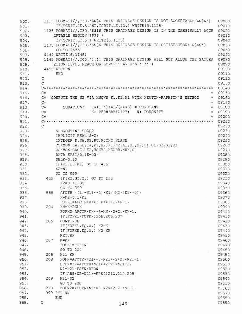
900. SOl. 902. 903. 904. 905. 906. 907. 908. 909. 910.
1115 FORMAT(//,T30,'$$$$ THIS DRAINAGE DESIGN IS NOT ACCEPTABLE$$$$') IF(TCRIT.GE.5.AND.TCRIT.LE.10.) WRITE(6,1125)
1125 FORMAT(//,T30,'$$$$ THIS DRAINAGE DESIGN IS IN THE MARGINALLY ACCE 2PTABLE REGION$$$$')
IF(TCRIT.LT.5.) WRITE(6,1135) 1135 FORMA~(//,T30,'$$$$ THIS DRAINAGE DESIGN IS SATISFACTORY$$$$')
GO TC 4455 4444 WRITE(6,1145) 1145 FORMAT(//,T40,' !!!! THIS DRAINAGE DESIGN WIL~ NOT ALLOW THE SATURA
2~ION LEVE~ REACH OR LOWER THAN 85% !!!! ') 4455 RETURN
09000 09010 09020 09030 09040 09050 09060 09070 09080 09090 09l.OO
911. END 09110 912. c 09l.20 913. c 09130 914. C******************************X***********~**************************** ·09140 915. 916.
918. 919. 920. 921. 922. 923. 924. 925. 926. 927. 92E. 929. 930. 932. .. 932. 933. 934. 935.
937. 935. 939. 940. 941. 942. 943. 944. 945. 946. 947. 948. 949. 950. 951. 952. 953. 954. 955. 956. 957. 958. 959.
C• C• COMPUTE THE N2 VIA KNOWN Kl,K2,N1 WITH NEWTON-RAPHSON'S METHOD C•
E;?UATICK: K•(l-N)••2/(N••3) =CONSTANT K: PERMEABILITY; N: POROSITY
* 09150 * 09150 * 09170 * 09180 •. 09190 * 09200
C*****************************X***************************************** 09210 09220 09230 09240 09250 09260
c
c
SUBROUTINE POR02 IMPLICIT REAL(J-Z) INTEGER N,NA,NB,NC,NJONT,NLANE COMMON ~A,RE,TA,Kl,K2,Nl,N2,A1,B1,B2,C1,Gl,G2,G3,Rl COMMON CASE,EED,HSUBA,HSUBB,NUM,S DATA EPSI/O.lE-03/ DELK=O.lO IF(K2.LE.Kl) GJ TO 455 IC=Nl GO TO 999
455 IF(K2.GT.O.) GO TC ~55
N2=0.E-05
555
204
205
207
206 208
209
GJ TO 999 AFCTR=((l.-Nl)••2)•Kl/(K2•(N~••J)) K=K2*0.l/Kl FOFKl=AFCTR*K*•3-K••2+2.•K-l. KN=K+DELK FOFKN=AFCTR•KN••3-KN**2+2. xl~N-2.. IF(FOFKl•FOFKN)206,205,207 CONTINUE IF(FOFKl.EQ.O.) N2=K IF(FOFKN.EQ.O.) N2=KN RETURN K=KN FOFKl=FOFKN GO TO 204 N2l=KN FOFN=AFCTR•N2l••3-N21••2+2.•N2l-l. DFDN=3.•AFCTR•N21••2-2.*N2l+2. N2=N21-FOFN/DFDN IF(ABS(N2-N2l)-EPSI)2l0,210,209 N21=N2 GO TO 208
210 FOFN2=AFCTR•N2•*3-N2•*2+2.•N2-l. 999 RETURN
END
145
09270 09280 09290 09300 09310 0932CJ 09330 09348 09350 093EO 0937U 09380 09390 094:JO 09410 09420 0943D 09440 09450 09460 09470 09480 09490 09500 095:'..0 09520 09530 09540 09550 09568 09570 09580 09590

960. c 09600 961. C*****************~*~****~~**~****************************************** 09610 962. 953. 964. 965. 966. 967. 966. 969. 970. 971. 972. 973. 974. 975. 976. 977. 976. 979. 980. 981. 982. 983. 984. 985. S86. 987. 936. 989. 990. S9l. 992. 993. 994. 9~15.
996. 99'7. 998. 999.
1000. lOC1. 1002. 1003. 1004. 1005. 1006. 1007. 1008. 1009. 1010. lOll. 1012. l0l3. 1014. 1015. 1016. 1017. 1018. 1019.
C* * 09620 * 09630 " 09640 * 09650 * 09660 * 09670
C* PRECIPITATION AS WELL AS DRY AND WET SEQUENCE C* C* GAMMA DISTRIBUTION FOR RAINFALL AMOUNT C* MARKOV CHAIN MODEL FOR DRY AND WET SEQUENCE C* C* READ THE RAINFALL AMOUNT AS WELL AS DRY AND WET SEQUENCE DA~A IN * C* INPUT MATERIAL PROPERTIES AND CHARACTERISTICS OF BASE AND SUBGRADE * C* COMPUTE THE ALPHA AND BETA OF GAMMA DISTRIBUTION *
09680 09690 09700
C* C* HALFT: TIME FOR 50% DRAINAGE(HOUR) C*
* 09710 " 09720 * 09730
C**~******~*********************T*************************************** 09740 09750 09760
c c
c c c c c c
c
c c
c c
c c
c c c
c c c
SUBROUTINE RAil'J(HALFT,IMAXD) IMPLICIT IN~EGER (I-N) DIMENSION ITITL2(20) DIMENSION AMT(5,300) ,SUM(10) ,N~M(lO) ,YDRAN(lOO) ,WPROE(50,50) COMMON /EDR/CONST,RECPOW,DURPOW,SHAPE COMMON /DRYWET/ TLAMDA,DRYLAM,WE~LAM,PWET COMHON /RAW/ X'IIM:C: (120, 10), YAREA (120, 10), INDS, TIMAX (10), UEMA.."l{ (10) COHMON /NOGAMA/ NUMWE~,AVGAMT,TOTSUM
READ THE RAINFALL A}!OUNT DATA IN l-~.ND COUNT THE NUMBER OF WET Dll.YS
09770 09780 09790 09800 09810 09820 09830 09840 09850 09860 09870
AMT(l): THE RAINFALL A~OUNT DURING THE PER!OJ IS CONCERNEJ (IN INCHES)098SC AMT(2): THE SEQUENCE OF DRY DAYS 09890 AMT(3): THE SEQUENCE OF WET DAYS 09900 !TYPE : TYPE OF PAVEMENT, EITHER FCC OR BCP 09910 ASOIL : SCIL TYPES CLASSIFIED EY 'AASHTO' OR 'UNIFIED'. BHORIZ: HORIZON (AE~ OR BC). P.b6,ASCE TRANS.ENGR.J.,JAN,l979 IBC INDEX OF BASE MATERIALS CRKJON: T~E LESGTH OF CRACKS AND JOINTS(IN FE~T) FROM FIELD SURVEY FTLONG: THE TOTAL LENGTH SURVEYED FOR CRACKS AND JOINTS YEAR ?HE EVALUED ?ERIOD IN YEARS CONST : CONSTANT 'K' FOR INTENSITY-DURATION-RECURRENCE EQUATION
DEFAULT = 0.3 RECPCW: PO~ER OF RECURRENCE IN~ERN~~( PERIOD EVALUATSD
DEFAULT = 0.25
09920 09930 09940 0995J 09960 09970 09980 09990 lC::)Q,:::, lC01C
DURPOW: POWER OF RAINFALL DURATION 10020 DEFAULT = 0.75 10030
SHAPE : THE CONSTANT DUE TO CilRVE SHAPE OF RA:NFALL IN~ENSITY VS. PERI1C04J DEFAULT = 1.65 (GAUSSIAN CURVE)
REAL*8 ASOIL INTEGER BHDRIZ
INPUT MATERIAL PROPERTIES OF BAE AND SUBGRADE
READ(5,445)IBC,ITYPE,ASOIL,BHORIZ 445 FORMAT(I4,A4,A8,A4)
READ(5,485)CRKJON,FTLONG 485 FORMAT(2Fl0.0)
READ(5,475)YEAR,CCNST,RECPOW,DURPOW,SHAPE 475 FORMAT(5Fl0.2)
IF(CONST.E~.O.) CONST=0.3 IF(RECPOW.EQ.O.) RECPOW=0.25
146
l005C 10060 10070 10080 10090 1c::..oc 10110 10120 10130 101~0
10150 10160 lCl70 lOlSO 10190

1020. 1021. 1022. 1023. 1024. 1025. 1026. 1027. 1028. 1029. 1030. 1031. 1032.
1034. 1035. 1036. 1037. 1038. 1039. 1040. l041. 1042. 1043. i044. 1045. 1045. 104'7. 1048. 1049. 1050. 1051. 1052. 1053. 1054. 1055. 1055.
1055. 1059. 1050. 1051. 1062. 1063. 1064. 1065. 1066. 1067. 1068. 1069. 1070. 1071. 1072. 1073. 1074. 1075. 1076. 1077. 1078. 1079.
c
IF(DURPOW.EQ.O.) DURPOW=0.75 IF(SHAPE.EQ.O.) SHAPE=l.65 WRITE(6,955)
955 FORMAT(1H1,T30, '***** PAVEMENT TYPES DATA AND PERIOD *****'///,1X, 2T20,'PVMT TYPE ',5X,'SOIL CLASS' ,5X,' HORIZON' ,6X,' CRK.JT. FT.', 35X,' SURVEYED FT' ,5X, I PERI08(YEAR) I,//)
WRITE(6,965)ITYPE,ASOIL,BHORIZ,CRKJON,FTLONG,YEAR 965 FORMAT(T20,A10,7X,A8,11X,A4,2(5X,F13.1) ,5X,F13.0,//)
Wr<ITE(6,455) 455 FORMAT(T30,'*****CHARACTERISTICS OF RAINFALL INTENSITY-DURATION-RE
2CURRENCE EQUATION*****' ,//,T30, 3'K(I-D-R EQ) I' I REC. POWER'! I DUR. POWER'' 4' CURVE SHAPE',//)
WRITE(6,465)CONST,RECPOW,DURPOW,SHAPE 465 FORMAT(T3C,4F13.2)
C READ !N RAINFALL DATA. ISEQ: 1,RA!NFALL AMOUNT EACH RAINY DAYF C 2,SEQUENCE OF DRY DAYS FREQUENCY C 3,SEQUENCE OF WET DAYS FREQUENCY c
c c
c
READ(5,985) IRAIN 985 FORMAT(I3)
DC 77777 ITIME=1,IRAIN READ(5,405) IT!TL2
405 FORMAT(2GA4) WRITE(6,495) ITITL2
495 FORMAT(1Hl,T30,20A4) DC 500 ISEQ=1,3
415
200 10'.:'
ND!': (I .SEQ) =0
DO 100 i...=l,20 INT=(L-1)*16H IEN=(L-l)rl6+l6 READ(5,415) (AMT(ISEQ,I) ,I=INT,IEN) Fom:AT(16F5.C)
DC 200 I=IN'I',IEN IF(AMT(ISEQ,I) .E~.O.) GO TC 500 lWl'! ( ISEQ) =:L
C:JNT I\' DE 500 CONTINUE
DO 800 IJ=2.,3 K=NUM ( IJ)
IF(K.EQ.O) K=1 IF(IJ.EQ.1) WRITE(6,915) NUM(1) IF(IJ.EQ.2) WRITE(6,925) NUM(2)
995 FORMAT(T40,16I5) IF(IJ.EQ.3) W~ITE(6,935) NJM(3)
905 FORMAT(T40,16F5.2) 915 FORMAT(//,T40,'***** RAINFALL AMOUNT DATA**~**',//,
2 T40,'NO. OF COUNTS=' ,IS,//) 925 FORMAT(//,T4D,'***** SEQUENCE OF DRY DAYS*****'//,
2 T40,'NO. OF COUNTS=' ,!5,//) 935 FORMAT(//,T40,'***** SEQUENCE OF WET DAYS*****',//,
2 T40,'NO. OF COUNTS=' ,IS,//) IF(IJ.KE.1) WRITE(6,995) (IFIX(AMT(IJ,I)) ,I=1,K)
TOTSUM: TOTAL NUMBER OF DAYS IN A PERIOD TOTNUM: TOTAL NUMBER OF corNTS FROM DRY AND WET DAYS' SEQUENCE
IF (I J. EQ. 1) '..Jrl I TE ( 6, 9 0 5) ( AMT (:!: J, I ) , I= 1 , K) BOO CONTINUE
C TEE AVERAGE ANG VARIANCE 147
10200 10210 10220 1Cl230 10240 1C250 10260 10270 10280 10290 10300 10310 10320 10330 10340 10350 10360 10370 10380 10390 10400 10410 10420 10430 10440 10450 10460 10470 10480 10490 10500 1052_0 10520
10540 l:J550 10560 10570 10580 10590 10508 10610 10620 10630 10540 10550 10650 10670 10580 10698 10700 10710 10720 10730 10740 10750 lJ760 l077::J 1078::J 10790

1080. 1081. 1082. 1083. 1084. 1085. 1086. 1087. 1088. 1089. 1090. 1091. 1092. 1093. 1094. 1095. J..096. 1097. 1Cl98. 1099. 2..100. 1101. 1102. 1103. 1104. 1105. ll06. l107. ll08. llJS. 1110. llll.
J..E3. E14. 2.ll5. 1116. 1117. 1118. 1119. 1120. :.121. 1122. 1123. 1124. 1125. 1126. 1127. ll28. 1129. ll30. 1131. 1132. 1133. J..134. 2.135. 1136. 1137. 1138. 1139.
c
c c c c c ,.... ·~
c c c
c c
DO 600 IB=l~3 SUM(IB)=O. IVALUE=NUM(IB) IF(IVALUE.EQ.O) IVALUE=1
DO 300 J=1 1IVALUE SUM(IB)=SUM(IB)+AMT(I8 1J)
300 CONTINUE 600 CONTINUE
NUMWET=NUM(1) IF(NUMWET.EQ.O) GC TO 333 AVGAMT=SUM(l)/NUM(l) GO TO 444
333 AVGAMT=O. 444 TOTNUM=NUM(2)+NUM(3)
TOTSUM=SUM(2)+SUM(3) AVGRAS=SUM(1)/TOT3UM IF(NUMWET.LE.1) GO TO 888 VRYLAM=TOTNUM/SUM(2) WETLAM=TOTNUM/SUM(3) ~LAMDA=DRYLAM+WETLAM
FwET=DRYLAM/TLAHDA PDRY=WETLAM/TLAMDA
AVGAMT: AVERAG2 OF AVGRAS: AVERP..GE CF 'iETLAM: RECIPROCAL DRYLAM: RECIPROCAL
ssAwr=o. DO 4CO K=1 1NUMWET
RAINFALL AMOUNT PER RAINY DAY RAINFALL AMOUNT PER DAY OF THE AVERAGE OF WET DAYS 0? THE AVERAGE OF DRY DAYS
400 SSAMT=SSAMT+(AKT(l 1K)-AVGAMT)••2 VARAMT=SSAMT/NUMWET
PARAMETERS GF GAMKA D!STRIBU~ION
AL?HA=AVGA~T••2/VARAMT EETA=AVGAMT/VARAMT
10800 10810 10820 10830 10840 10850 10860 10870 10880 10890 10900 10910 10920 10930 10940 10950 10960 10970 10980 10990 11000 11010 ll020 11030 11040 11050 11060 llC70 ll080 J.l090 lllOO 2..1110 11120 lL30 lll40 E2.5~;
2.2.l50
lll80 THE DURATION OF RAINFAL~(HOURS) CORRESPONDING TO AVERAGE RAINFALL AMOU1119C
WRITE(6 1945) 945 FORMAT(/// 1T30 1 '***** PARAMETERS OF GAMMA DISTRIBUTION AND MARKOV
2CHAIN MODEL*****') WRITE(6 1 435)AVGAMT 1 VARA~T 1 ALPHA 1 BETA
2 1DRYLAM 1WETLAM 1TLAMDA 1PDRY 1?WET 435 FORMAT(3(/), T40 1 'AVERAGE RAINFALL PER WET DAY(INCHES)
2 T40 1 'VARIANCE OF RAINFALL AMOUNT 3 // 1T40 1 'ALPHA OF GAMMA DISTRIBUTION 4 T40 1 'BETA OF GAMMA DISTRIBUTION 5 // 1T40,'LAMDA OF DRY DAYS (~ARKOV PROCESS) 6 T40 1'LAMDA OF WET DAYS (MARKOV PROCESS) 7 T40 1 'SUM OF LAMDA OF DRY AND WET DAYS 8 //,T40,'PROBABILITY OF DRY DAYS 9 T401'PROBABILITY OF WET DAYS
IF(TIHAX(INDS)/24.LT.l.) GQ TO 888 CALL KATZ ( IM~.XD, '1iPROB) CALL DRYDAY(IM~.XD 1 YDRAN 1 W?ROB)
= I , .F l G • 3 , I I
=' 1 F10.3 1 /,
='~F10.3 1 /I =' 1 ?10.3 1 /,
=' 1F10.3,/, =I I FlO. 3 I I I
=' 1F10.3 1/ 1 =' 1Fl0.3 1/l =' 1Fl0.3)
588 CALL FLOWIN(ALPHA,BETA 1PDRY 1PWET 1HALFT 1CRKJON 1IBC,ITY?E 1ASOIL 1 2BHORIZIF'!'LONG 1YEAR 1AVGRAS 1YDRAN 1WPROB 1IMAXD)
1 !l Q
ll20C 112l0 11220 ll230 ::..::..240
11260
11:280 2.l29J 11300 11310 ll320 1::..330
::..1340 ::..1350 ll36C 11370 ::.1380 ll390

1140. 1141. 1142. 1143. 1144. 114:5. 1146. :'..147. 1148. 1149. 1150. 1151. 1152. 1153. 1154. 1155. 1156. 1157. ll58. 1159. 1160. 1:61. 1162. ll63. 1164. 1165. 1166. 1167. li68. 12.59. 1170. 1171. 1::.72. 1:73. 1174. 1~75.
1175. 1177. 1178. 1179. 1180. ll8l. 1182. 1183. 1184. 1185. 1185. l:87. 1188. 1189. 1190. 1191. 1192. 1193. 1194. 1195. 1195. 1197. 1198. 1199.
77777 CONTINUE RETURN END
c C***************~*~*****************************************************
C• * C• SIMPSON¢S RULE USED TO INTEGRATE THE Gli.MMA DISTRIBUTION *
* C******~*******~*********~*****x****************************************
c c
c c c
,.., '--
SUBROUTINE S H1P2 (AREA2, GAHDIS ,XMIN ,XHAX, N, ALPHA, BETA) H=(XMAX-XMIN)/N SUM=O.O X=XMIN+H DO 4 I=2,N
IF(MOD(I,2))2,2,3 2 SUK=SUM+4.•GAMDIS(X,ALPHA,BETA)
GO TO 4 3 SUM=SUM+2.•GAXDIS(X,ALPHA,BETA) 4 X=X+H
,. ..
AREA2-=H/3. • ( GAMDIS (XlHK, ALPHA, BETA) +SUM+GAMDIS (XMAX, ALPHA, BETA)) RETURN
END
FUNCTION GAMDIS(X,AL?HA,BETA) EAS TO BE GREATER THAN 0. IN GAHKA DISTRIBUTION
IF(X.LE.O.AND.AL?HA.LE.1) GO TO 3333 GAMDIS=X••(ALPHA-1.)•EXPl-X•BETA)•(BETA••ALPEA)/(GAKMA(ALFHA)) RETURN
3333 GAKDIS=10.
c
F:ETU2N EKD
C*************************************************X******~****j:*********
C• * *
ll400 11410 11420 ll430 11440 11450 11450 11470 11480 11490 11500 11510 11520 11530 11540 11550 11!:50 11570 11580 11590 1l5JO 11510 11620 11530 11640 11650 11660 11670 ll630 1159()
ll71C 12.72G 11730 ll740
ll77C 117SC 11790 11800 C• SIMPSON'S RULE FOR IN~EGRATION
C• C• AREA: TEE AREA UNDER INTERGRATICN C• DUMMYF: FUNCTIONS; C• XKIN: MINIMUM VALUE OF Z C• XMAX: MAXIMUM VALUE OF X C• N: NUMBER OF SECTORS;
* 11810 * 11820 * 11830 * l1340 * 11850
* *
C*********************************************~*************************
c SUBROL'TINE SIHPSN (AREA, DUH!-!YF ,XHIN ,Xi!AX, N) INTEGER N,NA,NB,NC,NJONT,NLANE REAL LA,K1,K2,N1,N2 COHHON LA,HE,TA,K1,K2,N1,N2,A1,B1,B2,C1,Gl,G2,G3,R1 COMMON CASE,HED,HSUBA,HSUBB,NUM,S H= (XMAX-X!UN) /N SUH=O.O X=XKIN+H DO 4 I=2,N IF(MO~(I,2))2,2,3
149
11860 11870 ::..1880 11690 11900 11910 11920 11930 11940 11950 11960 119"70 11980 11990
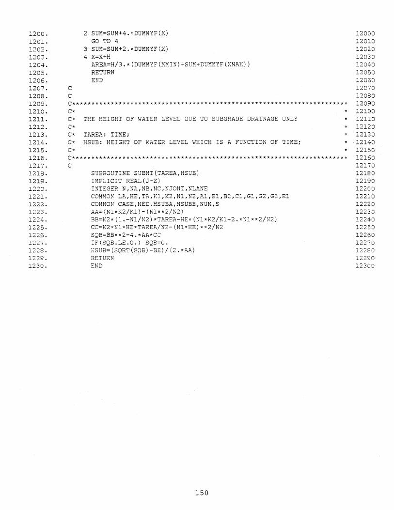
1200. 1201. 1202. 1203. 1204. 1205. 1206. 1207. 1208. 1209. 1210. 1211. 1212. 1213. 1214. 1215. 1216. 1217. 1218. 1219. 122:J. 1221. 1222. 1223. 1224. 1:225. 1226. 1227. 1228. 1229. 1230.
c c
2 SUM=SUM+4.~DUMMYF(X) GO TO 4
3 SUM=SUM+2.•DUMKYF(X) 4 X=X+H
AREA=H/3. • (DUI1MYF (XMIN) +SUK+DUKMYF (X.NAX)) RETURN END
C********************~********~*****************************************
12000 12010 12020 12030 12040 12050 12060 12070 12080 12090
C* ~HE HEIGHT OF WATER LEVEL DUE TO SUBGRADE DRAINAGE ONLY
C• ~AREJI.: TIME; C• HSUB: HEIGHT OF WATER LEVEL WHICH IS A FUNCTION OF TIME; C•
* 12100 * 12110 * 12120 * 12130 * . 12140 * 12150
c~*********************~************************************************ 12160 12l70 12180 12190 12200 12210 12220 12230 l2240 12250 12260 12270 12280 12290 l2300
c SUBROUTINE SUBHT(TAREA,HSUE) IMPLICIT REAL(J-Z) INTEGER N,NA,NB,NC,NJONT,NLANE COMMON LA,HE,TA,Kl,K2,N1,N2,A1,E1,B2,Cl,Gl,G2,G3,R1 COMMON CASE,HED,HSUBA,HSUBB,NUM,S AA=(N1•K2/K1)-(N1••2/N2) BB=K2•(1.-N1/N2)•TAREA-HE•(N1•K2/K1-2.•N1••2/N2) CC=K2•Nl•HE•TAREA/N2-(Nl•HE)~•2/N2 SQB=BB••2-4.•AA•CC :F(SQB.LE.O.) SQB=O. ESUB=(SQRT(SQE)-SE)/(2.•AA) RETURN END
150

1-' l.Jl 1-'
PROBLEM NUMBER ANALYSIS OF HOUSTON PAVEMENT IN MAY, 1970.
SYSTEM ANALYSIS OF RAINFALL INFILTRATION AND DRAINGE
LENGTH 75.00
HEIGHT 0.50
SLOPE FACTOR= 0.444
SLOPE% PERM. 1 1.50 10.00000
PERM.2 0.00000
PORO. 1 0. 1000
POR0.2 0.0100
NOTE: THE FOLLOWING ANALYSIS IS BASED ON PARABOLIC SHAPE PLUS SUBGRAOE DRAINAGE
HEAD ON X COOR. HT.(SUB.DRAIN ONLY) AVG. HEIGHT. TIME(STAGE 1 )
0.2500E 01 0.5000E 00 0.4944E 00 0.3788E-01 0.5000E 01 0.5000E 00 0.4889[ 00 0. 1452E 00 0.7500E 01 0.5000E 00 0.4833E 00 0.3108E 00 0. 1000E 02 0.5000E 00 0.4778E 00 0.5260E 00 0.1250E02 0.5000E 00 0.4722E 00 0.7839E 00 0. 1500E 02 0.5000E 00 0.4667E 00 0.1079E 01 0.1750E 02 0.5000E 00 0.4611E 00 0. 1407E 01 0.2000E 02 0.5000E 00 0.4556E 00 0. 1764E 01 0.2250E 02 0.5000E 00 0.4500E 00 0.2146E 01 0.2500E 02 0.5000E 00 0.4444E 00 0.2552E 01 0.2750E 02 0.5000E 00 0.4389E 00 0.2978E 01 0.3000E 02 0.5000E 00 0.4333E 00 0.3424E 01 0.3250E 02 0.5000E 00 0.4278E 00 0.3887E 01 0.3500E 02 0.5000E 00 0.4222E 00 0.4365E 01 0.3750E 02 0.5000E 00 0.4167E 00 0.4858E 01 0.4000E 02 0.5000E 00 0.4111E 00 0.5365E 01 0.4250E 02 0.5000E 00 0.4056E 00 0.5884E 01 0.4500E 02 0.5000E 00 0.4000E 00 0.6414E 01 0.4750E 02 0.5000E 00 0.3944E 00 0.6955E 01 0.5000E 02 0.5000E 00 0.3889E 00 0.7505E 01 0.5250E 02 0.5000E 00 0.3833E 00 0.8065E 01 0.5500E 02 0.5000E 00 0.3778E 00 0.8634E 01 0.5750E 02 0.5000E 00 0.3722E 00 0.9211E 01 0.6000E 02 0.5000E 00 0.3667E 00 0.9796E 01 0.6250E 02 0.5000E 00 0.3611E 00 0. 1039E 02 0.6500E 02 0.5000E 00 0.3556E 00 0. 1099E 02 0.6750E 02 0.5000E 00 0.3500E 00 0. 1159E 02 0.7000E 02 0.5000E 00 0.3444E 00 0. 1220E 02 0.7250E 02 0.5000E 00 0.3389E 00 0. 1282E 02 0.7500E 02 0.5000E 00 0.3333E 00 . 0. 1344E 02
DRAINAGE DEG.
0.1111E-01 0.2222E-01 0.3333E-01 0.4444E-01 0.5556E-01 0.6667E-01 0.7778E-01 0.8889E-01 0. 1000E 00 0.1111E 00 0. 1222E 00 0. 1333E 00 0.1444E 00 0.1556E 00 0. 1667E 00 0. 1778E 00 0. 1889E 00 0.2000E 00 0.2111E 00 0.2222E 00 0.2333E 00 0.2444E 00 0.2556E 00 0.2667E 00 0.2778E 00 0.2889E 00 0.3000E 00 0.3111E 00 0.3222E 00 0.3333E 00

HEAD ON Y COOR. HT.(SUB.DRAIN ONLY) AVG. HEIGHT TIME(STAGE 2) DRAINAGE DEG.
0.4833E 00 0.5000E 00 0.3222E 00 0. 1472E 02 0.3556E 00 0.4667E 00 0.5000E 00 0.3111E 00 0. 1605E 02 0.3778E 00 0.4500E 00 0.5000E 00 0.3000E 00 0.1744E02 0.4000E 00 0.4333E 00 0.5000E 00 0.2889E 00 0. 1890E 02 0.4222E 00 0.4167E 00 0.5000E 00 0.2778E 00 0.2043E 02 0.4444E 00 0. 4000E 00 0.5000E 00 0.2667E 00 0.2203E 02 0.4667E 00 0.3833E 00 0.5000E 00 0.2556E 00 0.2372E 02 0.4889E 00 0.3667E 00 0. 5000E 00 0.2444E 00 0.2550E 02 0.5111E 00 0.3500E 00 0.5000E 00 0.2333E 00 0.2738E 02 0.5333E 00 0.3333E 00 0.5000E 00 0.2222E 00 0.2936E 02 0.5556E 00 0.3167E 00 0.5000E 00 0.2111E 00 0.3147E 02 0.5778E 00 0.3000E 00 0.5000E 00 O.:>OOOE 00 0.3371E 02 O.GOOOE 00 0.2833E 00 0.5000E 00 0.1889EOO 0. 3611 E 02 0.6222E 00 0.2667E 00 0.5000E 00 0. 1778E 00 0.3867E 02 0.6444E 00 0.2500E 00 0.5000E 00 0. 1667E 00 0.4142E 02 0.6667E 00 0.2333E 00 0.5000E 00 0. 1556E 00 0.4439E 02 0.6889E 00 0.2167E 00 0.5000E 00 0. 1444E 00 0.4762E 02 0.7111E 00 0.2000E 00 0.5000E 00 0. 1333E 00 0.5113E 02 0.7333E 00 0. 1833E 00 0.5000E 00 0. 1222E 00 0.5499E 02 0.7556E 00 0. 1667E 00 0.5000E 00 0. 1111E 00 0.5926E 02 0.777BE 00 0. 1500E 00 0.5000E 00 0. 1000E 00 O.G402E 02 O.BOOOE 00
f-1 0. 1333E 00 0.5000E 00 0.8889E-01 0.6940E 02 0.8222E 00 U1 0. 1167E 00 0.5000E 00 0.7778E-01 0.7557E 02 0.8444E 00 N 0. 1000E 00 0.5000E 00 0.6667E-01 0.8276E 02 0.8667E 00
0.8333E-01 0.5000E 00 0.5556E-01 0.9135E 02 0.8889E 00 0.6667E-01 0.5000E 00 0.4444E-01 0. 1020E 03 0.9111E 00 0.5000E-Oi 0.5000E 00 0. 3333E·-01 0. 1158E 03 0.9333E 00 0.3333E-01 0.5000E 00 0.2222E--01 0. 1356E 03 0.9556E 00 0. 1667E-01 0.5000E 00 0. 1111E-01 0.1697E 03 0.9778E 00 0.8333E-02 0.5000E 00 0.5556E-02 0.2041E 03 0.9889E 00
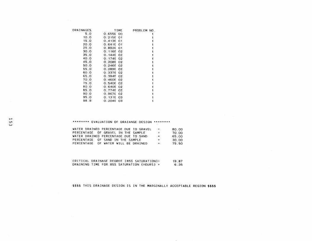
f-l lJl w
DRAINAGE% TIME PROBLEM NO. 5.0 0.655E 00 1
10.0 0.215E 01 15.0 0.413E 01 20.0 0.641E 01 25.0 0.892[ 01 30.0 0.116E02 35.0 0.144E02 40.0 0.174E02 45.0 0.208E 02 50.0 0.246E 02 55.0 0.289E 02 60.0 0.337E 02 65.0 0.394E 02 70.0 0.460E 02 75.0 0.540E 02 80.0 0.640E 02 85.0 0.774E 02 90.0 0.967E 02 95.0 0. 131E 03 98.9 0.204E 03
******** EVALUATION OF DRAIANGE DESIGN ********
WATER DRAINED PERCENTAGE DUE TO GRAVEL PERCENTAGE OF GRAVEL IN THE SAMPLE WATER DRAINED PERCENTAGE DUE TO SAND PERCENTAGE OF SAND IN THE SAMPLE PERCENTAGE OF WATER WILL BE DRAINED
CRITICAL DRAINAGE DEGREE (85% SATURATION)= DRAINING TIME FOR 85% SATURATION (HOURS) =
80.00 70.00 65.00 30.00 75.50
19.87 6.35
$$$$ THIS DRAINAGE DESIGN IS IN THE MARGINALLY ACCEPTABLE REGION $$$$

~
lJl .1::>
PVMT TYPE
BCP
***** PAVEMENT TYPES DATA AND PERIOD *****
SOIL CLASS HORIZON CRK.JT. FT. SURVEYED FT PERIOD( YEAR)
A-7-6 ABC 0.0 100.0 10.
*****CHARACTERISTICS OF RAINFALL INTENSITY-DURATION-RECURRENCE EQUATION*****
K(I-D-R EQ) REC. POWER OUR. POWER CURVE SHAPE
0.30 0.25 0.75 1.65

1-' Ul Ul
RAINFALL DATA AND ANALYSIS OF HOUSTON FAA AIRPORT; MAY, 1970.
**•** RAINFALL AMOUNT DATA*****
NO. OF COUNTS ~ 9
1.65 0.01 4.20 0.45 4.22 0.01 1.04 2.25 1.01
***** SEQUENCE OF DRY DAYS *****
NO. OF COUNTS = 4
8 4 4 6
***** SEQUENCE OF WET DAYS *****
NO. OF COUNTS = 5
2 3 2
***** PARAMETERS OF GAMMA DISTRIBUTION AND MARKOV CHAIN MODEL *****
AVERAGE RAINFALL PER WET DAY(INCHES) VARIANCE OF RAINFALL AMOUNT
ALPHA OF GAMMA DISTRIBUTION BETA OF GAMMA DISTRIBUTION
LAMDA OF DRY DAYS (MARKOV PROCESS) LAMDA OF WET DAYS (MARKOV PROCESS) SUM OF LAMDA OF DRY AND WET DAYS
PROBABILITY OF DRY DAYS PROBABILITY OF WET DAYS
********** TRANSITION PROBABILITY MATRIX **********
P00~0.781 P01 =0. 219
P10~0.536 p 11 =0. 464
1. 649 2.341
1 . 16 1 0.704
0.409 1.000 1. 409
0. 710 0.290

I-' Ul 0"1
PROBLEM NO. TIME(DAYS)
2
3
4
5
6
7
8
DRAINAGE(%) . PROB(CONSECUTIVE DRY DAYS)
49.24 0.710
71.35 0.554
83. 16 0.432
89.86 0.338
93.80 0.264
96. 11 0.206
97.67 o. 161
"100.00 0. 125

f-' lJl ---.)
WATER CARRYING CAPACITY OF BASE(SQ.FT)= AVERAGE DEGREE OF DRAINAGE PER HOUR OVERALL PROBABILITYT OF SATURATED BASE=
DRY PROBABILITY OF BASE COURSE WET PROBABILITY OF BASE COURSE
3.750 2.032 0.498
0.354 0.646
(THE ANALYSIS FOR WATER ENTERING PAVEMENT IS BASED ON DEMPSEY¢S FIELD EQUATION)
**********PROBABILITY DISTRIBUTION OF MODULUS OF BASE COURSE**********
SATURATION LEVEL (%) 10 20 30 40 50 60 70 80 90
WATER IN BASE(SQ.FT) 0.38 0. 75 1 . 13 1. 50 1 . 88 2.25 2.63 3.00 3.38
RAINFALL QT.(INCHES) 0.09 0.21 0.34 0.46 0.59 0.71 0.84 0.96 1.09
RAIN DURATION(HOURS) 0.00 0.00 0.02 0.07 0. 18 0.39 0. 75 1 . 31 2. 13
BASE MODULI (KSI) 64.60 64.60 64.60 64.60 64.60 64.60 29.36 19.00 5.07
RATIO OF DRY MODULUS 1 .00 1. 00 1 .00 1 .00 1 .00 1 .00 0.45 0. 29 0.08
SUBGRADE MODULI(KSI) 31 . 22 31.22 31.22 31 . 22 31.22 31.22 31.22 31 . 22 31 . 22
PROBABILITY DENSITY 0.45 0.48 0.47 0.46 0. 43 0.41 0.39 0.36 0.34
PROBABILITY 0.04 0.06 0.06 0.06 0.06 0.05 0.05 0.05 0.04
CUMULATIVE PROB. 0.04 0.09 0. 15 0.21 0.27 0.32 0.37 0.42 0.46
***** DISTRIBUTION CHARACTERISTICS OF RAINFALL EFFECT *****
AVERAGE FREE WATER IN BASE (SQ. FEET)= 1. 55
DURATION OF AVERAGE RAINFALL AMOUNT (HOURS)= 0.080
AVERAGE RAINFALL AMOUNT PER DAY (INCHES)= 0. 479'
AVERAGE BASE COURSE MODULUS IN WET STATE(KSI)= 25.84
AVERAGE BASE COURSE MODULUS (KSI)= 39.55
AVERAGE SUBGRADE MODULUS (KSI)= 31.22
100
3.75
1 . 2 1
3.29
2. 14
0.03
31. 22
0.31
0.04
0.50
(b) Water Penetration Into and Evaporation from a
Low Permeability Base Course
158

1. c 00010 2. C*********************************************************************** 00020 3. 4. 5. 6. 7. 8. 9.
10. ll,
12. 13. 14. 15. 16. 17. 18. 19. 20.
c C WATER INFILTRATION AND EVAPORATION OF A LOW PERMEABLE BASE COURSE c C TEXAS TRANSPORTATION INSTITUTE c c c
AUGUST 1983
* 00030 * 00040 * 00050 * 00060
* * *
C***********************************************************************
00070 00080 00090 00100 00110 00120 00130 00140 00150 00160 00170 00180 00190 00200 c
DIMENSION ASUBN(20),USOIL(50,50) ,SIGMA(20) ,ZROOT(20) DIMENSION EVWT(1000) ,SERIES(20) CALL LOWPER(DEPTH,INFILT) CALL EVAPOR(ZROOT,ASUBN,UATM,UNOT,DIFC,DEPTH,DQDU) CALL EVWET(ZROOT,ASUBN,UATM,UNOT,DIFC,DEPTH,DQDU) WRITE(6,115)
115 FORMAT (1H1) STOP END
21. ·c 00210 22. C*********************************************************************** 00220 23. 24. 25.
c C EVAPORATION OF WATER FROM SOIL WITH P. MITCHELL'S SOLUTION c
* 00230 * 00240 * 00250
26. C*********************************************************************** 00260 27. 28. 29. 30. 31. 32. 33. 34.
36. 37. 38. 39. 40. 41. 42. 43. 44. 45. 46. 47. 48. 49. 50. 51. 52. 53. 54. 55. 56. 57. 58. 59.
c C THIS SUBPROGRAM IS TO COMPARE THE SUCTION LEVELS OF DIFFERENT DEPTH C AT CERTAIN TIME IN ORDER TO CHECK WITH MITCHELL'S SOLUTION
c c c c c c c c c c c c c c c c c
SUBROUTINE EVAPOR(ZROOT,ASUBN,UATM,UNOT,DIFC,DEPTH,DQDU) DIMENSION ASUBN(20),USOIL(50,50) ,SIGMA(20) ,ZROOT(20)
UATM UNOT DIFC DEPTH YVERT EVTIHE: HRTIHE: DYTIHE: ASUBN : SIGHA : TSIGHA: USOIL ZROOT EVAPC DQDU
SUCTION OF ATHOSPHERE IN PF (LOG H) INITIAL SUCTION STATE OF SOIL IN PF DIFFUSION COEFFICIENT OF A SOIL (CH**2/SEC) WATER DEPTH IN SOIL (CM) VERTICAL DISTANCE FROM SOIL BOTTOH (CH) ELAPSED TIHE FOR EVAPORATION (SEC) ELAPSED TIHE FOR EVAPORATION (HOUR) ELAPSED TIHE FOR EVAPORATION (DAYS) COEFFICIENT OF FOURIER SERIES EVERY SINGLE TERH OF THE FOURIER SERIES TOTAL SUH FOR TEN TERHS OF FOURIER SERIES SOIL SUCTION IN DIFFERENT DEPTH AND TIHE (I2:DEPTH,I1:TIHE) ROOTS OF COTAN(Z)=Z/(DEPTH*EVAPC) EVAPORATION COEFFICIENT IN CH/SEC THE RATE OF WATER CONTENT CHANGE PER UNIT SUCTION (PF)
READ(5,305) UATH,UNOT,DIFC,DQDU,EVAPC 305 FORMAT(5E10.3)
WRITE(6,405)UATH,UNOT,DIFC,DQDU,EVAPC,DEPTH 405 FORMAT(1H1,///,T30, '********** EVAPORATION OF WATER FROM SOIL****
2******'' 3
4 5 6 7
8
//,T15, 'SUCTION OF ATMOSPHERE (PF) =' ,E10.3, //,T15,'INITIAL SUCTION OF SOIL (PF) =' ,E10.3, //,Tl5,'DIFFUSION COEFFICIENT (CM**2/SEC) =' ,E10.3, //,T15, 'SLOPE OF WATER CONTENT/ SUCTION =' ,E10.3, //,Tl5,'EVAPORATION COEFFICIENT (CM/SEC) =' ,E10.3, //,Tl5, 'DEPTH OF WATER PENETRATION (CM) =' ,E10.3)
159
00270 00280 00290 00300 00310 00320 00330 00340 00350 00360 00370 00380 00390 00400 00410 00420 00430 00440 00450 00460 00470 00480 00490 00500 00510 00520 00530 00540 00550 00560 00570 00580 00590

60. 61. 62. 63. 64. 65.
CALL EVROOT(ZROOT,DEPTH~EVAPC) DO 3000 I=1,10 ASUBN(I)=2.0*(UNOT-UATM)*SIN(ZROOT(I))/
2 (ZROOT(I)+SIN(ZROOT(I))*COS(ZROOT(I))) 3000 CONTINUE
WRITE(6,105)
00600 00610 00620 00630 00640 00650
66. 105 FORMAT(///,T30,'********* SUCTION DISTRIBUTION IN SOIL DUE TO EVAP 00660 67. 20RATION **********',3(/),T40,' TIME (DAYS)', 00670 68. 3T60,'SOIL DEPTH (CM) I I T80, 'SUCTION (PF) I ,3(/)) 00680 69. DO 3300 11=1,5 00690 70. 71. 72. 73. 74. 75. 76. 77. 78. 79. 80. 81. 82. 83. 84. 85. 86. 87. 88. 89. 90. 91. 92. 93. 94. 95. 96. 97. 98. 99.
100. 101. 102. 103. 104. 105. 106. 107. 108. 109. llO. lll. ll2. ll3. ll4. ll5. ll6. ll7. ll8. ll9.
c c
3100 3333
205 3200
2
DYTIME=Il*l. EVTIME=DYTIME*3600.*24.
D0-3200 I2=1,10 TSIGMA=O. YVERT=DEPTH/10.*I2
DO 3100 1=1,10 POWER=ZROOT(I)**2*EVTIME*DIFC/(DEPTH**2) IF(ABS(POWER).GE.100.) GO TO 3333
SIGMA(1)=ASUBN(I)*EXP(-ZROOT(I)**2*EVTIME*DIFC/ (DEPTH**2))*COS(ZROOT(I)*YVERT/DEPTH)
TSIGMA=TSIGMA+SIGMA(I) CONTINUE
USOIL(I2,I1)=UATM+TSIGMA WRITE(6,205) DYTIME,YVERT,USOIL(I2,I1) FORMAT(2(/),T40,F15.3,T60,F15.3,T80,E12.5) CONTINUE
3300 CONTINUE RETURN END
C***********************************************************************
c c c c
PERIODIC ROOTS FOR FOURIER SERIES OF WATER EVAPORATION FROM SOIL MODEL WITH P. MITCHELL'S SOLUTION
* * * *
C***********************************************************************
c c
c SUBROUTINE EVROOT(ZROOT,DEPTH,EVAPC)
C BISECTION METHOD TO SOLVE FOR ROOTS OF 'DEPTH*EVAPC*COT(Z)-Z=O' C DEPTH: LENGTH OF SOIL COLUMN IN CENTIMETER C EVAPC: EVAPORATION COEFFICIENT IN CM/SEC c
c
DIMENSION ZROOT(20) DATA EPSI/0.1E-05/ DO 1000 I=1,10
AMPLIT=EVAPC*DEPTH
C INPUT THE INITIAL VALUES ON BOTH SIDES (XL & XR) c
20
XL=3.1416*(I-1)+0.1 XR=3.14*I DO 100 IK=1,100 XM=(XL+XR)/2. FOFXL=AMPLIT*COTAN(XL)-XL FOFXM=AMPL1T*COTAN(XM)-XM IF(FOFXM*FOFXL) 20,30,40 XR=XM
160
00700 00710 00720 00730 00740 00750 00760 00770 00780 00790 00800 00810 00820 00830 00840 00850 00860 00870 00880 00890 00900 00910 00920 00930 00940 00950 00960 00970 00980 00990 01000 01010 01020 01030 01040 01050 01060 01070 01080 01090 01100 01ll0 01120 01130 01140 Oll50 01160 01170 01180 01190

120. 121. 122. 123. 124. 125. 126. 127. 128. 129. 130. 131. 132. 133. 134. 135. 136. 137. 138. 139. 140. 141. 142. 143. 144. 145. 146. 147. 148. 149. 150.
c c
30
40 50
100 210
2222 1000
GO TO 50 IF(FOFXM.EQ.O.) ZROOT(I)=XM IF(FOFXL.EQ.O.) ZROOT(I)=XL GO TO 2222 XL=XM IF(ABS(XL-XR)-EPSI) 210,210,100 CONTINUE ZROOT(I)=XM FZROOT=AMPLIT*COTAN(ZROOT(I))-ZROOT(I) CONTINUE
RETURN END
C***********************************************************************
c C WATER AMOUNT EVAPORATED FROM BARE SOIL c
* * *
C***********************************************************************
c c
SUBROUTINE EVWET(ZROOT,ASUBN,UATM,UNOT,DIFC,DEPTH,DQDU) DIMENSION ASUBN(20) ,EVWT(1000) ,SERIES(20) ,ZROOT(20)
C COMPUTATION OF AMOUNT OF WATER EVAPORATED FROM SOIL C EVWT WATER AMOUNT EVAPORATED FROM SOIL IN CM C SERIES: SINGLE TERM FOR THE FOURIES SERIES C TSERIE: SUM OF THE SERIES WHICH IS INTEGRATED FROM SUCTION AT c SPECIFIC TIME C DQDU THE RATE OF WATER CONTENT CHANGE PER UNIT SUCTION (PF) c
WRITE(6,405)
01200 01210 01220 01230 01240 01250 01260 01270 01280 01290 01~00
01310 01320 01330 01340 01350 01360 01370 01380 01390 01400 01410 01420 01430 01440 01450 01460 01470 01480 01490 01500
151. 405 FORMAT(1H1,2(/) ,T30,'*********** WATER AMOUNT EVAPORATED FROM SOIL 01510 152. 2 **********' ,3(/) ,T33, 'EVAPORATION TIME(HOUR) I ,T60, 'EVAPORATION AM 01520 153. 30UNT (CM) I, 3 (/)) 01530 154. DO 4100 IK=1,720 01540 155. TSERIE=O. 01550 156. HRTH!E=IK* l. 01560 157. 158. 159. 160. 161. 162. 163. 164. 165. 166. 167. 168. 169. 170. 171. 172. 173.
EVTIME=HRTIME*3600. DO 4000 I=1,10 POWER=ZROOT(I)**2*EVTIME*DIFC/(DEPTH**2) IF(ABS(POWER).GE.100.) GO TO 4411 SERIES(I)=ASUBN(I)*EXP(-ZROOT(I)**2*EVTIME*DIFC/(DEPTH**2))
2 *SIN(ZROOT(I))/ZROOT(I) TSERIE=TSERIE+SERIES(I)
4000 CONTINUE 4411 EVWT(IK)=(UATM-UNOT+TSERIE)*DEPTH*DQDU
c C OUTPUT THE RESULTp EVERY ~ HOURS c
I2=IK/2*2 IF(I2.NE.IK.AND.EVWT(IK) .LT.DEPTH) GO TO 4100 WRITE(6,415) HRTIME,EVWT(IK)
415 FORMAT(2(/),T45,F10.2,T60,F23.4) IF(EVWT(IK) .GE.DEPTH) GO TO 4444
01570 01580 01590 01600 01610 01620 01630 01640 01650 01660 01670 01680 01690 01700 01710 01720 01730
174. 4100 CONTINUE 01740 175. 4444 RETURN 01750 176. END 01760 177. c 01770 J..78. c 01780 179. C*********************************************************************** 01790
161

180. 181. 182.
WATER PENETRATION INTO A BASE COURSE OF LOW PERMEABILITY * 01800 * 01810 * 01820
183. C*********************************************************************** 01830 184. 185. 186.
c
c SUBROUTINE LOWPER(DEPTH,INFILT)
01840 01850 01860
187. C THIS SUBPROGRAM IS USED TO COMPUTE THE WATER DISTRIBUTION IN A LOW 01870 188. C PERMEABILITY BASE COURSE FROM THE CRACKS/JOINTS IN A PAVEMENT 01880 189. C EULER'S METHOD IS APPLIED AS A NUMERICAL ANALYSIS 01890 190. C UNITS: TIME - HOUR; LENGTH - CENTIMETER; 01900 191. C PERMEABILITY - CENTIMETER/HOUR 01910 192. C UNITS ARE FREE AS LONG AS THEY ARE CONSISTENT. ABOVE IS IN GENER01920 193. C WC WIDTH OF CCRACKS/JOINTS 01930 194. C TL DEPTH OF CRACKS/JOINTS 01940 195. 196. 197. 198. 199. 200. 201. 202. 203. 204. 205. 206. 207. 208. 209. 210. 211. 212. 213. 214. 215. 216. 217. 218. 219. 220. 221. 222. 223. 224. 225. 226. 227. 228. 229. 230. 231. 232. 233. 234. 235. 236. 237. 238. 239.
C HPERM C VPERM C DPWA C TIME C YOFT
HORIZONTAL PERMEABILITY OF BASE VERTICAL PERMEABILITY OF BASE DEPTH OF WATER LEFT IN CRACKS/JOINTS TIME PASSED FOR WATER PENETRATION VERTICAL DISTANCE INTO WHICH WATER INFILTRATES
C XOFT HORIZONTAL DISTANCE INTO WHICH WATER FLOWS C POR01 POROSITY OF BASE SOIL C INFILT: TIME FOR ALL WATER FROM CRACKS/JOINTS INFILTRATES INTO BASE c
c
DIMENSION DPWA(1000) ,TIME(1000) ,XOFT(1000) ,YOFT(1000),DL(1000) READ(5,25)WC,TL,HPERM,VPERM,POR01,HTCP
25 FORMAT(6(E10.3)) WRITE(6,45)
45 FORMAT(1H1,//,T30, '********** WATER DISTRIBUTION OF LOW PERMEABILI 2Y BASE COURSE **********' ,//)
WRITE(6,55)WC,TL,HPERM,VPERM,POR01,HTCP 55 FORMAT( //,T20,'WIDTH OF CRACK/JOINT (CM) =' ,E10.3,
2 //,T20, 'DEPTH OF CRACK/JOINT (CM) =' ,E10.3, 3 //,T20, 'VERTICAL PERMEABILITY OF BASE (CM/HR)=' ,E10.3, 4 //,T20,'HORIZONTAL PERMEABILITY OF BASE (CM/HR)=' ,E10.3, 5 //,~20,'POROSITY OF BASE COURSE =' ,E10.3, 6 //,T20, 'CAPILLARY HEAD OF BASE (CM) =' ,E10.3)
WRI'.!'E(6,65) 65 FORMA'.!'(///,13X,''.!'IME (HOUR) I ,5X, 'HORIZONTAL DIST. (CM) I,
27X, 'VERTICAL DIST. (CM) I ,4X,'CRACK WATER DEPTH(CM) I,//) DPWA(1)=TL YOFT(1)=0. TIME(1)=0. DELY=0.01 DO 100 I=2,1000 IH1=I-1 YOFT(I)=YOFT(IH1)+DELY DT=POR01*YOFT(I)*DELY/(VPERH*(YOFT(I)+HTCP+TL)) TIHE(I)=TIHE(IH1)+DT
XOFT(I)=SQRT(2.*HPERM*TIHE(I)*(TL+HTCP)/POR01) DENT=(HPERH*YOFT(I)*(TL+HTCP)/XOFT(I)+
2 VPERH*XOFT(I)*(YOFT(I)+TL+HTCP)/YOFT(I))*1.5708/POR01 DL(I)=(DENT*DT)/WC DPWA(I)=DPWA(IH1)-DL(I)
C OUTPUT ONE SET OF RESULTS OUT OF EVERY TEN CALCULATIONS
IF(DPWA(I) .LE.O.) GO TO 222 ID=IH1/10*10 IF(ID-IH1)100,111,100
162
01950 01960 01970 01980 01990 02000 02010 02020 02030 02040 02050 02060 02070 02080 02090 02100 02110 02120 02130 02140 02150 02160 02170 02180 02190 02200 02210 02220 02230 02240 02250 02260 02270 02280 02290 02300 02310 02320 02330 02340 02350 02360 02370 02380 02390
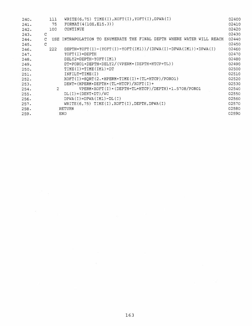
240. 241. 242. 243. c
111 WRITE(6,75) TIME(I) ,XOFT(I) ,YOFT(I),DPWA(I) 75 FORMAT(4(10X,E15.3))
100 CONTINUE
02400 02410 02420 02430
244. C USE INTRAPOLATION TO ENUMERATE THE FINAL DEPTH WHERE WATER WILL REACH 02440 245. 246. 247. 248. 249. 250. 251. 252. 253. 254. 255. 256. 257. 258. 259.
c 222 DEPTH=YOFT(I)-(YOFT(I)-YOFT(IM1))/(DPWA(I)-DPWA(IM1))*DPWA(I)
YOFT(I)=DEPTH DELY2=DEPTH-YOFT(IM1) DT=POROl*DEPTH*DELY2/(VPERM*(DEPTH+HTCP+TL)) TIME(I)=TIME(IM1)+DT INFILT=TIME(I) XOFT(I)=SQRT(2.*HPERM*TIME(I)*(TL+HTCP)/POR01) DENT=(HPERM*DEPTH*(TL+HTCP)/XOFT(I)+
2 VPERM*XOFT(I)*(DEPTH+TL+HTCP)/DEPTH)*1.5708/POROl DL(I)=(DENT*DT)/WC DPWA(I)=DPWA(IM1)-DL(I) WRITE(6,75) TIME(I) ,XOFT(I) ,DEPTH,DPWA(I)
RETURN END
163
02450 02460 02470 02480 02490 02500 02510 02520 02530 02540 02550 02560 02570 02580 02590

***~****** WATER DIS1RIBUTION OF LOW PERMEABILIY BASE COURSE **********
WIDTH OF CRACK/JOINT (CM) = 0.200E 01
DEPTH OF CRACK/JOINT (CM) = 0.250E 02
VERTICAL PERMEABILITY OF BASE (CM/HR)= 0.200E 00
HORIZONTAL PERMEABILITY OF BASE (CM/HR)= 0.200E-01
POROSITY OF BASE COURSE = 0. WOE 00
CAPILLARY HEAD OF BASE (CM) = 0.300E 03
TIME (HOUR) HORIZONTAL DIST.(CM) VERTICAL DIST.(CMi CRACK WATER DEPTH(CM)
0.846E-04 0.332E 00 0. WOE 00 0.250E 02 0.323E-03 0.648E 00 0.200E 00 0.249E 02 0.715E-03 0.964E 00 0.300E 00 0.248E 02 0. 126E-02 0. 128E 01 0.400E 00 0.246E 02 0. 196E-02 0. 160E 01 0.500E 00 0.244E 02 0.281E-02 0. 191E 01 0.600E 00 0.241E 02
f-1 0.382E-02 0.223E 01 0. 700E 00 0.238E 02 0'1 0.498E-02 0.::154E 01 0.800E 00 0.234E 02 ~ 0.629E-02 0.286E 01 0.900E 00 0.230E 02
0.775E-02 0.317E 01 0.100E 01 0.225E 02 0.937E-02 0.349E 01 0.110E 01 0.220E 02 0. 111E-01 0.381E 01 0. 120E 01 0.214E 02 0.131E-01 0.412E 01 0. 130E 01 0.208E 02 0.151E-01 0.444E 01 0. 140E 01 0.201E 02 0. 174E-01 0.475E 01 0. 150E 01 0.194E 02 0. 198E-01 0.507E 01 0. 160E 01 0.186E02 0.223E-01 0.538E 01 0. 170E 01 0.178E02 0.250E-01 0.570E 01 0. 180E 01 0. 169E 02 0.278E-01 0.601E 01 0.190E 01 0. 160E 02 0.308E-01 0.633E 01 0.200E 01 0. 150E 02 0.339E-01 0.664E 01 0.210E 01 0. 140E 02 0.372E-01 0.696E 01 0.220E 01 0. 130E 02 0.407E-01 0.727E 01 0.230E 01 0.118E02 0.443E-01 0.759E 01 0.240E 01 0. 107E 02 0.480E-01 0.790E 01 0.250E 01 0.945E 01 0.519E-01 0.822E 01 0.260E 01 0.819E 01 0.560E-01 0.853E 01 0.270E 01 0.688E 01 0.602E-01 0.884E 01 0.280E 01 0.551E 01 0.645E-01 0.916E 01 0.290E 01 0. 410E 01 0.690E-01 0.947E 01 0.300E 01 0.264E 01 0.737E-01 0.979E 01 0.310E 01 0.113E 01 0.772E-01 0. 100E 02 0.317E 01 0.112E-03

j-l
01 U1
********** EVAPORATION OF WATER FROM SOIL **********
SUCTION OF ATMOSPHERE (PF)
INITIAL SUCTION OF SOIL (PF)
DIFFUSION COEFFICIENT (CM**2/SEC)
SLOPE OF WATER CONTENT/ SUCTION
EVAPORATION COEFFICIENT (CM/SCC)
DEPTH OF WATER.PENETRATION (CM)
0.634E 01
0.397E 01
0.350E-04
0.200E 01
0.540E 00
0.317E 01
********* SUCTION DISTRIBUTION IN SOIL DUE TO EVAPORATION **********
TIME (DAYS) SOIL DEPTH (CM) SUCTION ( P F)
1.000 0. 317 0.43524E 01
1.000 0.635 0.43822E 01
1.000 0.952 0.44319E 01
1 .000 1. 269 0.45011E 01
1.000 1. 586 0.45896E 01
1.000 1. 904 0.46970E 01
1.000 2.221 0.48224E 01
1.000 2.538 0.49650E 01
1 .000 2.855 0.51233E 01
1.000 3. 173 0.52958E 01
2.000 0.317 0.48874E 01

2.000 0.635 0.49105E 01
2.000 0.952 0.49487E 01
2.000 1. 269 0.50017E 01
2.000 1. 586 0.50688[ 01
2.000 1. 904 0.51493E 01
2.000 2.221 0.52425E 01
2.000 2.538 0.53474E 01
2.000 2.855 0.54627E 01
2.000 3. 173 0.55874E 01
3.000 0.317 0.52835E 01
!--> 0"\ 3.000 0"\
0.635 0.53003E 01
3.000 0.952 0.53281E 01
3.000 1. 269 0.53667E 01
3.000 1. 586 0.54155E 01
3.000 1. 904 0.54742E 01
3.000 2.221 0.55420E 01
3.000 2.538 0.56183E 01
3.000 2.855 0.57022E 01
3.000 3. 173 0.57929E 01
4 000 0.317 0.55717E 01

4.000 0.635 0.55839E 01
4.000 0.952 0.56041E 01
4.000 1. 269 0.56322E 01
4.000 1. 586 0.56677E 01
4.000 1. 904 0.57104E 01
4.000 2.221 0.57597E 01
4.000 2.538 0.58151E 01
4.000 2.855 0.58762E 01
4.000 3. 173 0.59421E 01
5.000 0.317 0.57812E 01
I-> 0"1 5.000 0.635 0.57901E 01 -..]
5.000 0.952 0.58049E 01
5.000 1. 269 0.58252E 01
5.000 1. 586 0.58511E 01
5.000 1. 904 0.58821E 01
5.000 2.221 0.59180E 01
5.000 2.538 0.59583E 01
5.000 2.855 0.60027E 01
5.000 3. 173 0.60506E 01

*********** WATER AMOUNT EVAPORATED FROM SOIL **********
EVAPORATION TIME(HOUR) EVAPORATION AMOUNT (CM)
2.00 0.5339
4.00 0.9948
6.00 1 . 4172
8.00 1. 8123
10.00 2.1860
12.00 2.5422
14.00 2.8837
r-' 0"\ CXl 16.00 3.2123

E-3. GUIDE FOR DATA INPUT TO COMPUTER PROGRAM
(a) Simulation Model of Rainfall Infiltration
Drainage Analysis
and
1. Identification Card (IS, I3, 18A4)
2.
cc 1-5 IPROB
cc 6-8 INEED
cc ll-80 ITITLE
Characteristics
cc l-10 LA
cc ll-20 HE
cc 21-30 TAPER
cc 31-40 Kl
cc 41-50 K2
cc 51-60 Nl
cc 61-70 N2
of
Problem Number (~ 10)
Analytical procedures required
0: Drainage analysis only
1: Drainage analysis and
drainage design evaluation
2: System analysis of
rainfall infiltration and
drainage
Problem title
base and subgrade (7Fl0.0)
One side width of base (feet)
Depth of base (feet)
Slope ratio or value of tan
of base (%) e.g., tan a =
0.016, input 1.6
Permeability of Base
(Feet/Hour)
Permeability of Subgrade
(Feet/Hour)
Porosity of Base
Porosity of Subgrade*
169

*If N2 is not available, put 0.0 in columns 68-70,
N2 will be calculated by the equation
Kl (1-Nl) 2
(Nl) 3 = K2(1-N2) 2
(N2) 3
which is assumed that the base and subgrade are of the
same material.
NOTE: The following cards are needed only when INEED=l
and 2.
3. Material types of base course (2I5, 2Fl0.0)
cc 5 I TYPE Types of fines added*
1. Inert filler
2. Silt
3. Clay
cc 6-10 IQFINE Amount of fines added*
1. 0%
2. 2.5%
3. 5%
4. 10%
*see Table 2
cc 11-20 GRAVPC Percentage of Gravel in sample
e.g. 80%, Input 80.0
cc 21-30 SANDPC Percentage of Sand in sample
NOTE: If INEED=0 or 1, skip the following cards.
170

4. Material properties of base and subgrade (I 4, A4,
A8, A4)
cc 4 IBC Index of base course material
which corresponds to the
elastic modulus (see Table
3)
1. Crushed limestone+4% cement
2. Crushed limestone+2% lime
3. Crushed limestone
4. Gravel
5. Sand clay
6. Embankment-compacted
plastic clay
cc 5-8 I TYPE Pavement type (PCC or BCP)
cc 9-16 ASOIL Types of subgrade soils
classified by "AASHO" or
Unified (see Table 3)
cc 17-20 BHORIZ Horizon of subgrade (ABC or
BC)
5. Area of cracks and joints and surveyed field
length (2Fl0.0)
cc 1-10 CRKJON*
cc 11-20 FTLONG
linear length of cracks and
joints
(feet)
of one-side pavement
Surveyed field length (feet)
171

*If cracks and joints are not available
for CRKJON, the model will use
input
Dempsey
0.0
and
Robnett's regression equation to calculate the
amount of water flowing into base course.
6. Parameters of
equation (5Fl0.0)
cc l-10 YEAR
cc 11-20 CONST
cc 21-30 RECPOW
cc 31-40 DURPOW
cc 41-50 SHAPE
intensity-duration-recurrence
(see Appendix A-2)
Evaluated period (years)
Constant K (default=0.3)
Power of recurrence interval
(default=0.25)
Power of rainfall duration
(default=0.15)
Value corresponding to curve
shape of rainfall intensity
vs. rainfall period.
7. Number of rainfall amount and frequency data sets
(I 3)
cc l - 3 IRAIN Number of data set
The number of IRAIN means the number of different
periods will be evaluated for their climatic
effects on the same pavement and Cards 8-11 will
be used repeatedly.
172

8. Identification card for each season (20A4)
cc 1 -80 ITITL2 Title for the source of
rainfall data.
9. Rainfall amount data (16/5.0)*
AMT (ISEQ,l) Rainfall amount of each rainy
day (~0.01 inches)
10. Sequence of the number of dry days (16 F5.0)*
AMT (ISEQ,2) Number of consecutive dry days
in sequence**
11. Sequence of the number of wet days (16 F5.0)*
AMT (ISEQ,3) Number of consecutive wet days
in sequence**
*Every set of sequential data has to end with a
blank or zero. Three sets of data are in separate
cards.
**e.g., in a particular season, the sequence weather
is 5 dry days, 1 wet day, 4 dry days, 2 wet days,
2 dry days, .•• etc., then in
AMT (!SEQ, 2) input 5.0, 4.0, 2.0, .•• and in
AM T ( I s E Q I 3 ) input 1.0, 2.0,
173

(b) Water Penetration into a Base of Low Permeability
l. Characteristics of cracks/joints and the base
course (6E 10 0 3)
cc 1-10 we Width of Crack/Joint (em)
cc 11-20 TL Depth of Crack/Joint (em)
cc 21-30 HPERM Permeability of Horizontal
direction in Base Course
( cm/hr)
cc 31-40 VPERM Permeability of Vertical
direction in Base Course
(cm/hr)
cc 41-50 POROl Porosity of Base Course
(dimensionless)
cc 51-60 HTCP Capillary head in Base Course
(em)
2. Characteristics of water evaporation from the base
course and boundary conditions (5E 10.3)
cc 1-10 UATM
cc 11-20 UNOT
cc 21-30 DIFC
cc 31-40 DQDU
cc 41-50 EVAPC
Suction of atmosphere (pF)
Initial suction of base soil
(pF)
Diffusion
(cm2;sec)
Coefficient
Slope ratio between water
content and suction
Evaporation
(em/sec)
174
Coefficient