Envelope Computation in the Plane by ApproximateImplicitization

Tino SchulzJohannes Kepler University of Linz, Austria

tino.schulz@jku.at

Bert JuttlerJohannes Kepler University of Linz, Austria

bert.juettler@jku.at

Abstract

Given a rational family of planar rational curves in a certain region of interest, we are in-terested in computing an implicit representation of the envelope. The points of the envelopecorrespond to the zero set of a function (which represents the envelope condition) in the param-eter space combining the curve parameter and the motion parameter. We analyze the connectionof this function to the implicit equation of the envelope. This connection enables us to use ap-proximate implicitization for computing the (exact or approximate) implicit representation of theenvelope. Based on these results, we formulate an algorithmfor computing a piecewise algebraicapproximation of low degree and illustrate its performanceby several examples.

1 Introduction

The concept of anenvelope, which is a curve or surface that touches all members of a given familyof curves or surfaces, is useful in a variety of applications. In the theory of gearings, envelopes areused to find matching pairs of tooth flanks. In robotics, they are strongly related to the problem ofcollision detection, due to the close connection of the envelope and the swept volume of a movingsolid. Furthermore, envelopes are also of great interest ingeometrical optics and NC machining(caustics, path planning) and in Computer-Aided Design (offset curves and surfaces).

Envelopes of curves and surfaces and methods for computing them are discussed in the classicalliterature from kinematics and differential geometry, cf.[7, 19]. A survey on the topic is given in a pa-per by Pottmann and Peternell [22]. Abdel-Malek et al. [1] present several approaches for computingswept volumes. An algorithm for computing a boundary representation of swept volumes generatedby moving free-form surfaces is presented and discussed in [21].

Special classes of moving surfaces have been studied in moredetail. Kim et al. [18] considerswept volumes of moving polyhedra and Flaquer et al. [14] study envelopes of moving quadrics. Ina recent paper, Rabl et al. [23] analyze envelopes of moving surfaces which are characterized by aspecial form of their support function.

The envelope of a rational family of rational curves is generally not rational and its implicit rep-resentation is usually of high degree (compared to the degrees of the family). In particular, this is truefor offsets, which form an important subclass of envelopes. The offset of a curve can be obtained asthe envelope of the family of circles with fixed radius which move along the curve. It is well knownthat the class of algebraic curves and surfaces is closed with respect to the offsetting.

1

Due to their technical importance, the construction and analysis of offset curves has attractedthe attention of many researchers from fields of geometric design, algebraic geometry and symboliccomputation. In particular, a substantial number of publications discusses curves and surfaces withrational offsets, see [13] and the references cited therein. The existing literature also includes resultsconcerning offsets of general rational curves. For instance, the implicit equation of the offset curveswas shown to be useful for analyzing of topological changes of offset curves, see [2, 3, 4, 24].

Due to its potentially high degree, it is difficult to computethe implicit equation of general en-velopes. In order to address this difficulty, we propose to use the technique ofapproximate impliciti-zationfor envelope computation in this paper.

Given a parametric description of a curve (or surface), the process of finding the implicit de-scription is calledimplicitization. In the case of a rational parametrization, this conversionis alwayspossible, and the result is an algebraic hypersurface (curve in 2D or surface in 3D), represented asthe zero set of a polynomial (see [25, 27]). Several techniques for solving the implicitization problemare available, e.g. Grobner bases, moving curves/surfaces, or methods based on resultants (cf.[6, 12]and [17]). While planar curves can be handled efficiently with these approaches, their application tosurfaces is problematic due to the increased computationalcomplexity. in practice, the use of exactmethods for implicitization is only reasonable for surfaces of low degree. Furthermore, the varietyprovided by the exact implicitization may contain branchesand self-intersections that the user wouldhave liked to avoid for certain reasons.

The idea ofapproximate implicitization[8] is to generate an approximation (of low degree) of theexact algebraic representation, which represents the shape of the given curve or surface in the regionof interest. Using approximate implicitization it is possible to avoid the difficulties associated withthe exact method.

In this paper we will restrict ourselves to the case of a family of planar, rational curves, followingthe approach introduced by Dokken (cf. [8, 10]). A comparative benchmarking of this technique andof other methods for approximate implicitization may be found in [28] and [31]. Since we are aimingat a local (rather than a global) approximation and on numerical evaluation, we will mainly use theweak formulation of approximate implicitization [9, 11]. It will be shown that the algebraic error ofthe approximation of the envelope is bounded in a similar wayas in the original approach.

This paper is organized as follows. The next two sections recall the concepts of approximateimplicitization and envelope computation, respectively.The fourth section introduces the combinationof both concepts. Based on these results, we present an algorithm for computing a piecewise, algebraicapproximation of a family of rational curves in Section 5. Moreover, several examples will illustrateits performance. Finally we conclude this paper.

2 Approximate implicitization

We recall the classical version of approximate implicitization (AI) and its weak formulation. We alsogive an outline of how to deal with interpolation constraints in this framework. See [8, 9, 10, 11] foradditional details.

2.1 Dokken’s first method

Consider a segment of a planar rational parametric curves 7→ p(s), s∈ I , of degreen, where thecompact intervalI ⊂ R is the parameter domain. We assume that this curve segment iscontained in abounded open subsetΩ ⊂ R

2, which we call the region of interest.

2

In order to approximatep(s), s∈ I , by an algebraic curve, which is defined as the zero set

q−1(0) = p ∈ Ω : q(p) = 0 (1)

of a bivariate polynomialq : R2 → R of degreem, we consider the composition

(qp)(s) = q(p(s)). (2)

The polynomialq has a representation of the form

q(x) =(m+2

2 )

∑i=1

βi(x)ci = cTβ (x) (3)

where the functionsβi are a basis of the space of bivariate polynomials of maximum degreemand theci ∈R are the coefficients with respect to it. We collect the coefficients in the coefficient vectorc of qand the basis functions in another vectorβ (x).

The first approach to approximate implicitization is based on a factorization of the composition(2),

(qp)(s) = q(p(s)) = (Dc)Tα(s), (4)

where the vectorα(s) = (α0(s), . . .αmn(s))T contains a basis of the polynomials of maximum degreemn in s, which is non-negative and forms a partition of unity onI . For instance, one may take theBernstein polynomials on the intervalI . The matrixD, which is determined by the given curve andby the chosen basisα , hasmnrows and

(m+22

)

columns.In order to eliminate the parameters (and hence to implicitize the given curve), Dokken considers

the norms of the vectors and matrices in (4). For alls∈ I we have that

∑i(αi(s))

2 ≤ ∑i

αi(s) = 1, (5)

hence‖α(s)‖ ≤ 1, where‖.‖ is the usual Euclidean norm of vectors. Thus,

maxs∈I

|q(p(s))| = maxs∈I

|(Dc)Tα(s)| (6)

≤ ‖Dc‖maxs∈Ω

‖α(s)‖ ≤ ‖Dc‖. (7)

An approximate implicitization of the given curve can now befound by minimizing‖Dc‖ subject to‖c‖= 1. The latter constraint is needed in order to exclude the trivial solution.

The solutionc can be found efficiently by performing a singular value decomposition (SVD) ofD (see [16]) and choosing the singular vector corresponding to the smallest singular valueσmin. Thisgives

‖Dc‖ ≤ σmin.

Summing up, the approximate implicitization is defined by the bivariate polynomial ˜q with coefficientvectorc. This polynomial satisfies

maxs∈I

|q(p(s))| ≤ σmin. (8)

This result possesses the following geometric interpretation: The given curve segmentp(s) with s∈ Iis contained in the “fat” algebraic curve

q−1([−σmin,σmin])∩Ω = x ∈ Ω : −σmin ≤ q(x)≤ σmin. (9)

3

This region of the plane is bounded by the two algebraic offset curvesq(x) =−σmin andq(x) = σmin.In particular, if the matrixD possesses the singular value zero, then the corresponding singular vectorgives the coefficients of an exact implicitization of the given rational curve.

As shown by Dokken, approximate implicitization possessesa high order of approximation. Thus,the error converges to zero very quickly if the length of the interval I is decreased. However, themethod certainly only considers metric aspects. Additional considerations need to be taken into ac-counct to certify, that the approximate implicitization possesses the correct topology, cf. [26].

As a problem for the implementation and practical usage of approximate implicitization, the nu-merically stable computation of the matrixD in (4) is relatively complicated, requiring compositionalgorithms for polynomials in Bernstein-Bezier form. In addition, the number of entries grows quitefast withm. Also, the technique is not suitable for approximate implicitization by spline functionsq,since the space of functions generated by the compositionsqp depends on the given curve and doesnot possess a simple basis.

2.2 Weak approximate implicitization

In order to avoid these computational difficulties, the weakmethod for approximate implicitization(cf. [9]) considers directly the basisβ (x), which was already introduced in (3), and integrates thesquared residualsq(p(s)) over the intervalI ,

∫

Iq(p(s))2ds=

∫

I

(

cTβ (p(s)))2

ds= cTMc, (10)

with the symmetric matrix

M =

∫

Iβ (p(s))β (p(s))Tds. (11)

Clearly, one may use numerical methods for evaluating the integrals.Note that the choice of the basisβ depends on the region of interestΩ, which reflects the local

character of the weak approach. For instance, one may consider the Bernstein-Bezier polynomialswith respect to a triangle containing the region of interest.

The weak approximate implicitization of the given curve is found by minimizing the objectivefunction defined in (10) subject to the constraint‖c‖ = 1. Similar to the original method, SVD canbe used to find the solution ˜q with the coefficient vectorc. The value of (10) is equal to the smallestsingular valueσmin of M .

Since we are considering a compact intervalI and the space of polynomials of degreemndefinedon it, there exists a constantC (depending on the degreemnand onI , but not on the given curve) suchthat

maxs∈I

|q(p(s))|= ‖qp‖∞ ≤C‖qp‖2 =C√

σmin, (12)

where the norms‖.‖2 and‖.‖∞ are theL2 and the maximum norm of polynomials inI . Thus, the weakapproximate implicitization admits a similar geometric interpretation as the original approach, cf. (9).

2.3 Interpolation constraints

Additional interpolation constraints, which force the approximate implicitization to match a certainnumber of given points, can be added either before or after the SVD.

Consider the first possibility. Suppose that we want our approximation to interpolate a pointp0.Following the weak approach, this gives the condition

q(p0) = cTβ (p0) = 0. (13)

4

Using a Lagrangian multiplier, one is led to apply the SVD to the modified matrix

M =

(

M β (p0)β (p0)

T 0

)

, (14)

and then to omit the last entry of the singular vector.As a second method, one may compute a linear combination of the singular vectors ofM which

are associated with the smallest singular values, in order to satisfy the interpolation condition(s). Inthe remainder of the paper we will use the first (Lagrange-multiplier-based) interpolation method.

3 Envelopes

The envelope of a family of curves is a curve which touches each member of the family. Followingthe approach in [22], we will use a spatial interpretation todescribe this property. First we explain thisin the case of an implicitly defined family of curves, and thenwe proceed to the case of parametriccurves.

3.1 Implicitly defined curves

We consider a family of real, planar curves which are defined as the zero sets of a trivariate polynomialF(p, t), wherep = (p1, p2) ∈ Ω ⊂ R

2 are the coordinates andt ∈ J ⊆ R is the time-like parameteridentifying the members of the family. The domainΩ represents the region of interest, and the time-like parametert varies in an intervalJ ⊂R. For each constant valuet = t0, the set of points satisfyingF(x, t0) = 0 forms a planar curve. Ast varies inJ, we obtain a one-parameter family of curves.

Let ∂t denote the partial differentiation with respect tot. The envelopeD of the family is definedas

D = p ∈ Ω : ∃t ∈ J : F(p, t) = ∂tF(p, t) = 0. (15)

Note that the setD may be empty and that in this case no real part of the envelope exists.This definition can be understood with the help of the following spatial interpretation, see Fig. 1.

The equationF(p, t) = 0 defines a surfaceS in three-dimensional space with coordinatesp = (p1, p2)andt. The intersections with the planest = constant, give – after projecting them orthogonally intothe(p1, p2)-plane – the curves which belong to the family. We will denotethis orthogonal projectionby π.

The set of all points of the surfaceSsatisfying∂tF(x, t) = 0 forms thecontourwith respect to theprojectionπ, and their image is thesilhouetteof the surface. The tangent planes of the surface alongthe contours are projected into lines, since their normal vectors are perpendicular to the direction ofprojection.

For any pointP= (p, t0) of the contour, we consider the intersection curve with the planet = t0through this point. Both this curve and the contour touch thetangent plane at the pointP. Thus,the projections – which are the curve of the family and the envelope – possess the same tangent atp = π(P), which is obtained as the image of the tangent plane.

Therefore we can think of an envelope as the silhouette of a surface underπ. The contour – whichis projected into the silhouette – is defined as the intersection of the two surfacesF = 0 and∂tF = 0.The implicit equation of the envelope can be found by eliminating t from both equations.

5

t

S

Contour

SilhouetteFigure 1: Spatial interpretation of envelopes:The contour of the surfaceS is projected intothe silhouette. Simultaneously, this gives the en-velope of the family of curves obtained by pro-jecting the intersections ofS with planest =constant into the(p1, p2)-plane.

3.2 Parametric curves

In this paper we are mainly interested in the case of a rational family of rational curves. More precisely,we consider a family of curves

p(s, t) =(

x(s, t)w(s, t)

,y(s, t)w(s, t)

)T

, (s, t) ∈ I ×J (16)

wherex, y andw are bivariate polynomials of degree(n1,n2) with gcd(x,y,w) = 1 and the domain isthe Cartesian product of two closed intervalsI ,J ⊂R. We assume thatw(s, t) 6= 0 for all (s, t) ∈ I ×J.For each constant value of the second (time-like) parametert = t0, we obtain a segment of a rationalcurves 7→ p(s, t0) with domainI .

We consider the embedding

p(s, t) =(

x(s, t)w(s, t)

,y(s, t)w(s, t)

, t

)T

(17)

of the family of curves into the three-dimensional space with coordinates(p1, p2) andt.In order to find an implicit equation of the envelope, one could proceed as follows: First one

might compute at-dependent implicit equation of the formF(p, t) = 0, i.e. an implicit equation of thesurfacep. Second, one could derive the implicit equation as described in the previous section. Thisapproach – which requires the elimination of three variables – is fairly complicated, and we prefer towork directly with the parametric representation.

As in the previous section, we are interested in thecontourof the surfacep with respect to theparallel projectionπ. The contour consists of all points whose normal vector is parallel to the(p1, p2)-plane. The third coordinate of the normal vectors∂sp×∂t p is the rational functionh(s, t)/w(s, t)3 withthe numerator

h(s, t) = det

x(s, t) ∂sx(s, t) ∂tx(s, t)y(s, t) ∂sy(s, t) ∂ty(s, t)w(s, t) ∂sw(s, t) ∂tw(s, t)

. (18)

The zero setZ = h−1(0) of this bivariate polynomialh defines the points inI ×J which correspond tothe envelope.

6

We will refer toh(s, t) as theenvelope functionand toh(s, t) = 0 as theenvelope condition. Notethat h is independent of the choice of the third coordinate ofp, i.e. for any embedding of the form(p1, p2,z(s, t))

T with an arbitrary functionz(s, t), the envelope function is the same. This is due to thefact that all these embeddings generate the same silhouette.

If a rational parameterization(s(ξ ), t(ξ )) of the curve defined byh(s, t) = 0 were available,we could obtain a parametric descriptionk(ξ ) of the envelope by composing it withp, k(ξ ) =p(s(ξ ), t(ξ )). However, the envelope condition does not define a rational curve in general.

The envelope functionh equals the numerator of the Jacobian determinant ofp. Indeed, theenvelope consist of the singular points of the mappingp (cf.[5]). Thus singularities of the specificparametrization are a part of the envelope andh necessarily depends on the parametrization.

4 Approximate implicitization of envelopes

We present a modification of weak approximate implicitization which is well suited for the computa-tion of envelopes. More precisely, we consider the following problem.

Given a family of rational curves (16), find an approximate implicit representation of the envelope.Several possible approaches exist, which we list below.

1. One could implicitize the surfacep(s, t) (see (17)) in order to obtain an implicit representationF(p, t) = 0 of the family of curves. It is then possible to use the technique outlined in Section3.1, i.e., to find the implicit equation of the envelope by eliminatingt from F = 0 and∂tF = 0.Generally, the degree ofF will be rather high, making this method impractical.

Applying approximate implicitization top is also inadequate, since one first has to compute asurfaceand then compute its contour to get the envelopecurve.

2. Sometimes it may be possible to find a (rational) parameterization of the curve represented bythe envelope conditionh(s, t) = 0. By composing it with the parametric representation of thefamily of curves one then obtains a parametric representation of the envelope. This possibility israther theoretical, since the curveh(s, t) = 0 can generally not be parameterized by elementaryfunctions (in the sense of [29]) and it is generally not knownhow to generate such a parametriza-tion, except for rational [27] or square-root parametrizations [30]. Also, this approach wouldgive a parametric representation of the envelope, instead of an implicit one.

3. An implicit equationq(x) = 0 of the envelope can also be derived directly by eliminatingtheparameterss, t,T from the four equations

Xw(s, t)−x(s, t) = 0, Yw(s, t)−y(s, t) = 0, h(s, t) = 0,T w(s, t) = 1, (19)

wherex = (X,Y)T . The last equation with the new variableT ensures thatw(s, t) does notvanish. We will present a special approximate technique forperforming this elimination.

4.1 Jacobian embedding

Motivated by the system of equations (19), we define another embedding of the family of curves as

p(s, t) =(

x(s, t)w(s, t)

,y(s, t)w(s, t)

,h(s, t)

)T

. (20)

7

t

Contour

Silhouette

h

Contour

Silhouette

Figure 2: Transforming the embeddingp (left) into the Jacobian embeddingp (right): The points onthe contour are pushed into the plane, but the silhouette of the surface (which is simultaneously theenvelope of the family of curves) remains the same.

We call it theJacobian embedding, since the third coordinate is the numerator of the Jacobiandeter-minant of the mappingp.

By comparing this embedding with the spatial interpretation from section 3, one realizes that theJacobian embedding possesses the same silhouette (envelope), since the envelope condition does notdepend on the choice of the third coordinate. Moreover, all points that satisfy the envelope conditionare embedded in the(p1, p2)-plane. Consequently,the zero contour of the Jacobian embeddingpequals its silhouette, hence the envelope.

As an example, Figure 2 shows the original embeddingp of a family of curves and the Jacobianembeddingp.

The (approximate) implicit equationq(x) = 0 of the envelope could be found in the two steps of (1)(approximately) implicitizing the Jacobian embedding and(2) restricting the result to the points wherethe third coordinate is equal to zero. Consequently, the most direct approach is the use of approximateimplicitization for finding a low degree approximation ˜q(x,h) of the Jacobian embedding. The curveq(x,0) gives an approximation of the envelope. However, this situation is similar to the approximateimplicitization of p. In order to find ˜q, one has to compute an approximate implicitization of asurface,although we are only interested in thecurveobtained as the intersection of that surface with the planeh= 0. Instead of this direct approach, we suggest to couple the envelope condition with the parametricrepresentation in a different way, which is described in thenext section.

4.2 Implicitization and the envelope function

When approximating the envelope of a rational familyp with an algebraic curveq= 0, it is naturalto consider their compositionq p. Now there is a difference to the standard case of approximateimplicitization: even for the exact equation of the envelope, we getq(p(s, t)) = 0 only for specificvalues ofsandt, which are determined by the envelope functionh.

In this section, we consider the family of curves and its envelope in the complex affine planeC2.The envelope function possesses a factorization

h(s, t) =M

∏i=1

hi(s, t)ki (21)

8

in C[s, t] with relatively prime, irreducible factorshi and multiplicitieski ∈ Z+. We say thathi is aproper factor of the envelope function if the image of the algebraiccurvehi(s, t) = 0 – considered inthe complex affine planeC2 – under the rational mappingp does not degenerate into a single point.Otherwisehi is said to beimproper.

Any improper factor hi of the envelope function is characterized by the fact that the directionalderivative ofp along the tangent vectors ofhi = 0 is the null vector. Consequently, improper factorscan be found in two steps. First one computes the squarefree representation

h(s, t) =M

∏i=1

hi(s, t) (22)

of the envelope function. Second, one finds the greatest common divisor of the two numerator poly-nomials in

−(∂t h)(∂sp)+ (∂sh)(∂tp) (23)

and the squarefree representationh of the envelope function. This gcd is the product of all improperfactors.

We consider thereduced envelope function

h(s, t) = ∏i=1,...,M

hi is proper

hi(s, t) (24)

which is obtained by eliminating all improper factors and redundant powers of proper ones. Theimage of the algebraic curveh(s, t) = 0 under the rational mappingp is said to be theproper partof the envelope. Note that this may include complex components that were not considered in theprevious discussion.

In addition to its proper part, the envelope consists of several (possibly complex) points, whichare obtained as the images of the algebraic curveshi(s, t) = 0 defined by improper factors underp.These points are either contained in almost all curves of thefamily, or one of these curves degeneratesinto this single point. We illustrate the situation by a simple example.

Example 1 We consider the family of circles through the point(0,1)T that touch the x-axis. It pos-sesses the rational parameterization

p =

(

(s+ t)(st+1)1+s2 ,

s2(1+ t2)

1+s2

)T

. (25)

Its envelope functionh= (t + I)(t − I)s(1+st) (26)

possesses the three improper factors h1 = t + I, h2 = t − I and h4 = 1+ st. The algebraic curvesh1 = h2 = h4 = 0 are mapped to the three points(I ,0), (−I ,0) and (0,1). The first two points areobtained as degenerate circles for t=±I, while the third point is contained in almost all circles. Theonly proper factorh= h3 = s is mapped to the envelope, which is the zero set of the linearpolynomalq(X,Y) =Y. It satisfies

(qp)(s, t)w(s, t) = (1+ t2)h3(s, t)2. (27)

Therefore, the reduced envelope function appears with multiplicity 2 in qp.

We show that this observation is true in general:

9

Theorem 1 Let p(s, t) =(

x(s,t)w(s,t) ,

y(s,t)w(s,t)

)Tbe a rational family of planar rational curves, with w(s, t) 6≡

0. Let q(x) = 0 be the square-free implicit equation of the proper part of the envelope and let d be itsdegree. There exists a bivariate polynomial g(s, t) such that

(qp)(s, t)w(s, t)d = g(s, t) h(s, t)2.

Proof 1 The proper part of the envelope consists of all pointsp(s, t) satisfyingh(s, t) = 0and w(s, t) 6=0. Each proper factor hi defines a (not necessarily real) component of the envelope. Since (qp)(s, t)) = 0 holds for the infinite number of points satisfying hi(s, t) = 0, we conclude that hi is afactor of the numerator of qp.

We show that h2i is a factor of the numerator of(q p), provided that hi is proper. Since hi issquarefree, it suffices to show that

[∇st(qp)](s0, t0) = 0 (28)

for all points(s0, t0) ∈C2 satisfying hi(s0, t0) = 0. Here∇st denotes the gradient with respect to(s, t).

Almost all points satisfying hi(s0, t0) = 0 are regular (i.e. (∇sthi)(s0, t0) 6= 0). We consider allpoints satisfying∂thi(s0, t0) 6= 0. Unless hi(s, t) is a scalar multiple of(t − t0), this covers almost allpoints on hi(s0, t0) = 0. For each one of them, there exists a local regular parameterization σ →(σ , t(σ)), whereσ varies in a certain open neighborhood of s0 in the complex planeC. For almostall points among them, the correponding local parameterization of the envelopeσ 7→ p(σ , t(σ)) isregular at s0, i.e.

(

ddσ

p(σ , t(σ))

)

(s0) = (∂sp)(s0, t0)+ (∂tp)(s0, t0) t ′(s0) 6= 0, (29)

as the algebraic curve hi = 0 was assumed to be a proper component of the envelope function. Sincethe algebraic curve q= 0 covers all proper components of the envelope, we have that

0=d

dσ[qp(σ , t(σ))] = (∇xyq)(p(s0, t0)) · [(∂sp)(s0, t0)+ (∂tp)(s0, t0) t ′(s0)]. (30)

On the one hand, the vector(∂sp)(s0, t0)+ (∂tp)(s0, t0)t ′(s0) is not the null vector, since the param-eterization was assumed to be regular(29). On the other hand, the two vectors(∂sp)(s0, t0) and(∂tp)(s0, t0) are linearly dependent, as h(s0, t0) = 0. Consequently,

0= (∇xyq)(p(s0, t0)) · (∂sp)(s0, t0) = (∇xyq)(p(s0, t0)) · (∂tp)(s0, t0) (31)

which implies(28). The case where hi is a scalar multiple of t− t0 can be dealt with similarly.

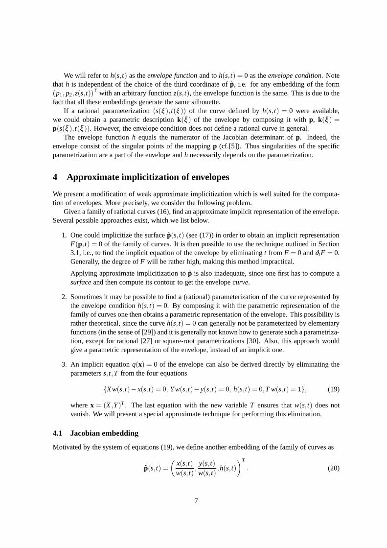
This result admits the following simple geometric interpretation: Consider the Jacobian embed-ding p along with the implicit equation of the envelopeq. At regular intersection points with the planeh = 0, the tangent plane of this embedding is orthogonal to the planeh = 0. In three-dimensionalXYh-space, the equationq(X,Y) = 0 defines a generalized cylinder which touchesp at all points inthe planeh= 0, since the Jacobian embedding has vertical tangent planesthere.

4.3 Coupled method for approximate implicitization of envelopes

Theorem 1 motivates us to find the approximate implicitization q of the envelope curve as an approx-imate solution of the equation

(qp)wm = λh2, (32)

10

where bothq andλ are unknown. More precisely,λ is another polynomial in(s, t) ∈ I × J, the freeparameterm is the degree ofq andw is the denominator ofp.

The polynomialq approximates the implicit equation of the envelope, while the auxiliary polyno-mial λ simultaneously approximates the factorg in theorem 1. We compute an approximate solutionof (32) by minimizing the objective function

F =∫

I×J

(

q(p(s, t))w(s, t)m−λ (s, t)h(s, t)2)2d(s, t), (33)

that couples the compositionq p with the envelope functionh. We will refer to λ as couplingfunction.

Let q(x) be of degreem andλ (s, t) of bidegree(k1,k2). After choosing basesα(s, t) andβ (x)of the bivariate polynomials of degreem and bidegree(k1,k2), respectively, we may represent theunknown polynomials as

q(x) = cTq β (x) and λ (s, t) = cT

λ α(s, t). (34)

After substituting them into the objective function (33) wearrive at

F =∫

I×J

(

cTγ)2, (35)

where

c=(

cq

cλ

)

and γ =

(

w(s, t)mβ (p(s, t))−h(s, t)2α(s, t)

)

. (36)

The minimizer of (35) subject to‖c‖2 = 1 can be found by applying SVD to the matrix

M =

∫

I×JγγT . (37)

The first (m+ 1)(m+ 2)/2 entries of the solution vector are the coefficients of the approximatingcurveq= 0. Interpolation conditions (e.g., interpolation of points) can be incorporated by introducingconstraints on this part of the solution.

Theorem 2 Consider the rational family(16) of rational curves. We assume that the denominatorw satisfies|w(s, t)| ≥ ε for a positive constantε , for all (s, t) ∈ I × J. Let c be the unit vector whichcorresponds to the smallest singular valueσmin of M , q= 0 be the corresponding algebraic curve andλ be the coupling function, respectively. We consider the envelope function h and its zero set

H = (s, t) ∈ I ×J : h(s, t) = 0.

Thenmax

(s,t)∈H

|q(p(s, t))| ≤C√

σmin,

where C is a positive constant which depends only onε , I ,J and on the degrees ofp, q andλ .

Proof 2 For any compact set S and any function f: S→ R , let ‖ f‖∞,S be the supremum of f on S.Due to|w(s, t)| ≥ ε > 0 we have in particular,

max(s,t)∈H

|q(p(s, t))| = ‖qp‖∞,H . (38)

11

and moreover, there exists a positive constantC∈ R such that

‖w−m‖∞,H ≤ C. (39)

This leads to

‖qp‖∞,H = ‖(qp)wmw−m‖∞,H ≤ ‖w−m‖∞,H ‖(qp)wm‖∞,H

≤ C ‖(qp)wm‖∞,H . (40)

Recall thatH ⊂ I ×J and‖h‖∞,H = 0. Therefore

‖(qp)wm‖∞,H = ‖(qp)wm− λh2‖∞,H ≤ ‖(qp)wm− λh2‖∞,I×J. (41)

Since I×J is compact, there exists a positive constantC ∈ R which depends solely on the degrees ofthe polynomials q,p, λ and on the intervals I,J, such that

‖(qp)wm− λh2‖∞,I×J ≤ C ‖(qp)wm− λh2‖2,I×J, (42)

where‖.‖2,I×J is the L2 norm of a function on I×J. Sincec minimizes (35),

(‖(qp)wm− λh2‖2,I×J)2 = σmin. (43)

Combining(38) and (40)–(43) we get

max(s,t)∈H

|q(p(s, t))|= ‖qp‖∞,H ≤C√

σmin, (44)

where C∈ R is a positive constant depending onε , I ,J and the degrees ofp, q, λ .

Thus,all points of the envelope are contained in an algebraic offset of the approximating curve.This geometric interpretation of the result is analogous tothe case of weak approximate implicitiza-tion.

We demonstrate the performance of our method by a first example.

Example 2 Consider the family of curves which is shown in Fig. 3. This isa family of bidegree(1,3)and the exact envelope is an algebraic curve of degree 10. Thefamily of linesp has been derived byslightly perturbing the coefficients of the family of tangents of a planar cubic.

Fig. 4 shows the results of two approximate implicitizations with conics (m= 2) and cubics(m= 3). In both cases we used bilinear coupling functions. Note that the exact solution (dashedcurve) possesses a self-intersection, which is not reproduced by the low-degree approximate solutions.

5 Piecewise approximate implicitization of envelopes

In principle, the presented method is capable of computing the exact implicit equation of the envelope.However, the degrees needed for that are generally rather large. For example, if the familyp isdescribed by a bivariate, quadratic polynomial, then the envelope functionh is in the generic case ofbidegree(3,3). Thus the implicit equation of the Jacobian embedding can have a maximal degree2 ·3 ·3 = 18 and the same is true for the implicit equation of the envelope. Since we want to satisfyqp = λh2, both degrees of the coupling functionλ need to be 2·18−2·3= 30.

In total we get12(19·20)+312 = 1151 degrees of freedom. Solving such a high degree problem iscomputationally expensive, since it requires the construction and SVD of a 1151×1151 matrix. Forpractical purposes, a piecewise approximation by low degree curves is more useful.

12

Figure 3: Example 2. A cubic family of lines(grey), their control polygon and the region of in-terest (dashed box) which is used for the approxi-mate implicitization in Fig. 4.

5.1 The Algorithm

As before, we are considering a (rational) family of rational curves (cf. (16)). Without loss of gen-erality we can assume thatI × J = [0,1]× [0,1]. Let the degrees ofp be (n1,n2). We describep inBernstein-Bezier representation:

p(s, t) =∑i, j pi j wi j B

n1i (s)Bn2

j (t)

∑i, j wi j Bn1i (s)Bn2

j (t), (45)

with Bnk(z) =

(nk

)

(1−z)kzn−k andpi j ∈ R2,wi j ∈ R,0≤ i ≤ n1,0≤ j ≤ n2.

We formulate an algorithm which computes an approximation of the envelope curve by pieces ofalgebraic curves. The segments of the curves are joined continuously at their end points. Moreover,if the envelope curve possesses different branches in the region of interest, then all of them will beapproximated.

The algorithm is based on two assumptions onh:

(i) The envelope functionh is squarefree and does not possess improper factors.

(ii) The zero set ofh has no singularities inI ×J.

The first assumption is needed for the stability of the numerical computations, which are per-formed by using floating point numbers, and in order to use Theorem 1. If improper factors arepresent, then the algorithm can still be executed, but it maynot give optimal results.

As a possible extension of our approach, one might use a factorization ofh and gcd computationsin order to identify the reduced envelope functionh. This extension, however, requires special tech-niques for polynomials with coefficients given by floating point numbers, cf. [15]. The degree of the

13

without boundary conditions withC0 boundary conditions

m=

2m=

3

Figure 4: Example 2. Approximate implicitization of the family of lines from Fig. 3. In addition tothe family of curves (grey), the figure shows approximationsof the envelopes for degreesm= 2,3and(k1,k2) = (1,1) (black, solid) and the exact envelopes (dashed). The circles mark the segmentend points of the envelope in the region of interest. The curves in the right column interpolate thesepoints.

approximation segments and the degrees of the coupling functions are the free parameters. We denotethem withmand(k1,k2), respectively.

The main idea of the approach is a recursive subdivision of the parameter domainI ×J into four(squared) subdomains. We use a minimum recursion depthr ≥ 0 in order to control the detection ofsmall closed loops which may be part of the envelope. Thus, each box in the parameter domain whichcontains a part of the zero set ofh has at most a diameter of 2−r

√2.

The algorithm consists of four steps:

1.) Compute the Bernstein-Bezier representation of the envelope function, denoting its coefficientmatrix withH.

2.) If the entries ofH are either all positive or all negative, then no envelope exists in this domain(convex hull property) and the algorithm terminates. Otherwise continue with step 3.

3.) Compute all real intersection points(sl , tl ) of h(s, t) = 0 with the boundaries of the considereddomain. Collect the coordinatesp(sl , tl ) in a setS .

4.) If |S | = 2 andr ≤ 0 compute an approximate implicitization of the envelope, interpolating thepoints inS and using degreesm and(k1,k2) (cf. Section 4.3). Otherwise, subdividep into fourparts and apply the algorithm to each of them, usingr −1 as their minimum recursion depth.

In our current implementation, the computation in step 3 is performed numerically. Alternativelyone might be using Sturm sequences or the variation diminishing property of the Bernstein-Bezierrepresentation ofh to certify the number of intersections.

14

5.2 Discussion

The recursive subdivision stops, if after at leastr steps exactly two solutions ofh= 0 are found on theboundary of the currently considered parameter domain. Dueto the previous assumptions onh, thealgorithm always terminates in the generic case. Problems may occur if the zero set ofh incidentallytouches one of the boundaries of the boxes generated by the subdivision. In the generic case this doesnot occur.

We aim to approximate always just one (part of a) branch of theenvelope with one algebraic curve.If closed loops of the zero set ofh are contained in one subdomain, then each of them contributes anadditional branch to the envelope. Since we perform at leastr subdivision steps, all loops with adiameter which is bigger than 2−r

√2 are found. Loop detection is a well known problem and has

been extensively studied (see for example [20]).There is no special treatment of singularities of the envelope. Usually, after some subdivisions,

the approximation interpolates at least one point close to the singularity. The segments are connectedat these points and theirC0-transition mimics the behavior of a cusp point.

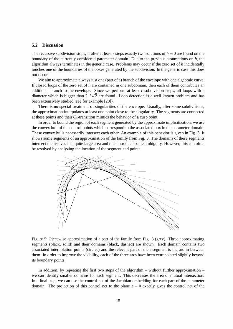
In order to bound the region of each segment generated by the approximate implicitization, we usethe convex hull of the control points which correspond to theassociated box in the parameter domain.These convex hulls necessarily intersect each other. An example of this behavior is given in Fig. 5. Itshows some segments of an approximation of the family from Fig. 3. The domains of these segmentsintersect themselves in a quite large area and thus introduce some ambiguity. However, this can oftenbe resolved by analyzing the location of the segment end points.

Figure 5: Piecewise approximation of a part of the family from Fig. 3 (grey). Three approximatingsegments (black, solid) and their domains (black, dashed) are shown. Each domain contains twoassociated interpolation points (circles) and the relevant part of their segment is the arc in betweenthem. In order to improve the visibility, each of the three arcs have been extrapolated slightly beyondits boundary points.

In addition, by repeating the first two steps of the algorithm– without further approximation –we can identify smaller domains for each segment. This decreases the area of mutual intersection.In a final step, we can use the control net of the Jacobian embedding for each part of the parameterdomain. The projection of this control net to the planez= 0 exactly gives the control net of the

15

corresponding part of the parameter domain. Now we compute the three-dimensional convex hullCH(p) of the control net of the Jacobian embedding. Due to its definition, all points of the envelopemust be contained in the intersection of CH(p) with the planez= 0. This reduces the domain for eachapproximating segment even further.

It may happen that single segments of the approximation consist of unconnected branches. Sofar, no part of the algorithm prohibits an approximation with separate branches. In our experience theunconnected, interpolating segments typically get connected after some subdivision steps. However,this issue is a common feature of most methods for approximate implicitization.

The values fork1,k2 should depend on the value ofm and a good choice for them is hard to makein general. However, so far we experiencedk1 = k2 = mgiving good results in our test cases.

5.3 Examples

We will illustrate the performance of the algorithm by several examples. The algebraic curves wereplotted via a predictor-corrector method, using the interpolation points (circles) as initial values.

Example 3 Offsets of a parabola. If the distance is chosen high enough,the offset of a parabolacontains a “swallowtail” in one of its branches. This part ofthe offset contains two cusps and oneself-intersection. In Fig. 6, the relevant part of an offsetand approximations with conics of differentsubdivision levels are depicted. Furthermore, the corresponding parameter domains are shown toillustrate the subdivision process.

Example 4 WV-shaped curve. We used cubic splines and cubic coupling functions to approximate arational family of rational curves of bidegree(3,2) (see Fig. 7). The subdivision clearly improves thereproduction of singularities and gives connected segments.

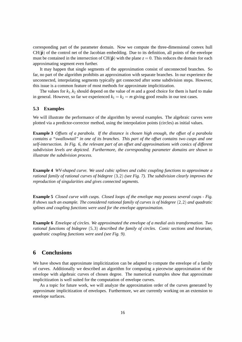
Example 5 Closed curve with cusps. Closed loops of the envelope may possess several cusps - Fig.8 shows such an example. The considered rational family of curves is of bidegree(2,2) and quadraticsplines and coupling functions were used for the envelope approximation.

Example 6 Envelope of circles. We approximated the envelope of a medial axis transformation. Tworational functions of bidegree(5,3) described the family of circles. Conic sections and bivariate,quadratic coupling functions were used (see Fig. 9).

6 Conclusions

We have shown that approximate implicitization can be adapted to compute the envelope of a familyof curves. Additionally we described an algorithm for computing a piecewise approximation of theenvelope with algebraic curves of chosen degree. The numerical examples show that approximateimplicitization is well suited for the computation of envelope curves.

As a topic for future work, we will analyze the approximationorder of the curves generated byapproximate implicitization of envelopes. Furthermore, we are currently working on an extension toenvelope surfaces.

16

Curves and envelope approximation Parameter domain and zero set ofhr=

0r=

1r=

2r=

3

Figure 6: Example 3. Approximation of an offset of a parabola. The family of curves consists ofcircular arcs with constant radius, which are centered along a parabola. In each row a piecewiseapproximation with conics (m= 2,(k1,k2) = (2,2)) and their corresponding parameter domains areshown. In addition, the zero set of the envelope function is plotted. Each circle on the left side isinterpolated and corresponds to a diamond on the right. The minimum recursion depth isr = 0,1,2,3,respectively.

17

Curves and envelope approximation Parameter domain and zero set ofh

r=

1r=

2

Figure 7: Example 4. Approximate implicitization of an envelope curve consisting of several brancheswith cubic curves (m= 3, (k1,k2) = (3,3)). The right side shows the corresponding parameter do-mains and the zero set of the envelope function. Each branch of this curve gives one branch of theenvelope. First row (r = 1): Several segments are unconnected and the singularitiesare not repro-duced properly. Second row (r = 2): Further subdivision gives connected segments and an improvedapproximation of the singularities.

18

r = 2 r = 3

Figure 8: Example 5. Loops of envelopes usually contain several cusps. In this example the degreeswerem= 2 and(k1,k2) = (2,2), so the segments cannot contain singularities. Left (r = 2): The cuspsare not represented very well, since the segment end points are too far away. Right (r = 3): After anadditional subdivision step some segment end points are close to the cusps, so that the singularitiesare approximated well.

Figure 9: Example 6. Piecewise approximation of the envelope generated by a medial axis trans-formation with 53 segments using the degreesm= 2 and(k1,k2) = (2,2). The right picture showsa enlarged version of the dashed region in the left one. Note the dense distribution of interpolationpoints near the singularities.

19

Acknowledgments. This research has been supported by the Austrian Science Fund (FWF) in theframe of the FSP S092 “Industrial Geometry”, subproject 2. The authors would like to thank JosefSchicho and the referees for their useful comments which have helped to improve the manuscript.

References

[1] K. Abdel-Malek, J. Yang, D. Blackmore, and K. Joy. Swept volumes: fundation, perspectives,and applications.International Journal of Shape Modeling, 12(1):87–127, 2006.

[2] J. Alcazar. Good global behavior of offsets to plane algebraic curves. Journal of SymbolicComputation, 43(9):659–680, 2008.

[3] J. Alcazar, J. Schicho, and J. Sendra. A delineability-based method for computing critical setsof algebraic surfaces.Journal of Symbolic Computation, 42(6):678–691, 2007.

[4] J. Alcazar and J. Sendra. Local shape of offsets to algebraic curves.Journal of Symbolic Com-putation, 42(3):338–351, 2007.

[5] V. Arnold, S. Gusein-Zade, and A. Varchenko.Singularities of differentiable maps. Springer,1985.

[6] C. Bajaj. The emergence of algebraic curves and surfacesin geometric design.Directions inGeometric Computing, pages 1–28, 1993.

[7] O. Bottema and B. Roth.Theoretical Kinematics. Dover Publications, 1990.

[8] T. Dokken. Approximate implicitization.Mathematical methods for curves and surfaces, Oslo2000, pages 81–102, 2001.

[9] T. Dokken, H. Kellermann, and C. Tegnander. An approach to weak approximation implicitiza-tion. Mathematical Methods for curves and surfaces, Oslo 2000, pages 103–112, 2001.

[10] T. Dokken and J. Thomassen. Overview of approximate implicitization. In Topics in Alge-braic Geometry and Geometric Modeling: Workshop on Algebraic Geometry and GeometricModeling, July 29-August 2, 2002, Vilnius University, Lithuania, volume 334, pages 169–184.American Mathematical Society, 2003.

[11] T. Dokken and J. Thomassen. Weak approximate implicitization. InIEEE International Confer-ence on Shape Modeling and Applications, 2006. SMI 2006, pages 204–214, 2006.

[12] M. Elkadi and B. Mourrain. Residue and implicitizationproblem for rational surfaces.Applica-ble Algebra in Engineering, Communication and Computing, 14(5):361–379, 2004.

[13] R. Farouki. Pythagorean-Hodograph Curves: Algebra and Geometry Inseparable. Springer,2008.

[14] J. Flaquer, G. Garate, and M. Pargada. Envelopes of moving quadric surfaces.Computer AidedGeometric Design, 9(4):299–312, 1992.

[15] A. Galligo and M. van Hoeij. Approximate bivariate factorization: a geometric viewpoint. InProc. Int. Workshop on Symbolic-Numeric Computation, pages 1–10. ACM, 2007.

20

[16] G. Golub and C. Van Loan.Matrix computations. The Johns Hopkins University Press, 1996.

[17] C. Hoffmann. Implicit curves and surfaces in cagd.IEEE Computer Graphics and Applications,13(1):79–88, 1993.

[18] Y. Kim, G. Varadhan, M. Lin, and D. Manocha. Fast swept volume approximation of complexpolyhedral models.Computer-Aided Design, 36(11):1013–1027, 2004.

[19] E. Kreyszig.Differential Geometry. Dover, 1991.

[20] N. Patrikalakis and T. Maekawa.Shape interrogation for computer aided design and manufac-turing. Springer Verlag, 2002.

[21] M. Peternell, H. Pottmann, T. Steiner, and H. Zhao. Swept volumes. Computer-Aided DesignAppl, 2:599–608, 2005.

[22] H. Pottmann and M. Peternell. Envelopes-computational theory and applications. InSpringConference on Computer Graphics, pages 3–23. Comenius University, Bratislava, 2000.

[23] M. Rabl, B. Juttler, and L. Gonzalez-Vega. Exact envelope computation for moving surfaces withquadratic support functions. In Lenarcic and Wenger, editors, Advances in Robot Kinematics:Analysis and Design, pages 283 – 290. Springer, 2008.

[24] F. San Segundo and J. Sendra. Partial degree formulae for plane offset curves.Journal ofSymbolic Computation, 44(6):635–654, 2009.

[25] T. Sederberg. Planar piecewise algebraic curves.Computer Aided Geometric Design, 1(3):241–255, 1984.

[26] T. Sederberg, J. Zheng, K. Klimaszewski, and T. Dokken.Approximate implicitization usingmonoid curves and surfaces.Graphical Models and Image Processing, 61(4):177–198, 1999.

[27] J. Sendra, F. Winkler, and S. Perez-Diaz.Rational algebraic curves. Springer, 2007.

[28] M. Shalaby, J. Thomassen, E. Wurm, T. Dokken, and B. Juttler. Piecewise approximate implic-itization: Experiments using industrial data. In B. Mourrain, M. Elkadi, and R. Piene, editors,Algebraic Geometry and Geometric Modeling, pages 37–52. Springer, 2006.

[29] D. Shanks.Solved and unsolved problems in number theory. AMS Chelsea Pub., 1993.

[30] M. Van Hoeij. An algorithm for computing the Weierstrass normal form. InProc. Int. Symp.Symbolic and Algebraic Computation, pages 90–95. ACM, 1995.

[31] E. Wurm, J. Thomassen, B. Juttler, and T. Dokken. Comparative benchmarking of methods forapproximate implicitization. In M. Neamtu and M. Lucian, editors, Geometric Modeling andComputing: Seattle 2003, pages 537–548. Nashboro Press, Brentwood, 2004.

21