Journal of Computational and Applied Mathematics 213 (2008) 294–299www.elsevier.com/locate/cam

Letter to the Editor

Enumeration results for Runge–Kutta methods for index 2 DAEsFrank Cameron

Tampere University of Technology/Pori, P.O. Box 300, 28101 Pori, Finland

Received 10 February 2006; received in revised form 18 December 2006

Abstract

Recursive formulas are presented that give the number of order conditions for single-step Runge–Kutta methods for index 2 DAEs.© 2007 Elsevier B.V. All rights reserved.

MSC: 65L06; 05C30

Keywords: Runge–Kutta methods; Index 2 DAEs; Order conditions; Enumeration

1. Introduction

To design a Runge–Kutta (RK) method for numerically solving an index 2 DAE, one needs order conditions (OCs).As the number of OCs is often large, it makes sense to generate them automatically [2]. When automatically generatingan array containing OCs, we have two options for handling the array size: (i) increase the size ‘on-the-fly’ via dynamicmemory allocation or (ii) pre-allocate the array to its correct size. Option (ii) is computationally more efficient, but touse it we must know the number of OCs beforehand. This paper contains recursive enumeration formulas for OCs forindex 2 DAEs. Although the enumeration formula for ODEs is about 150 years old [4, p. 154], it is believed that theindex 2 formulas given in Section 2 are new. The remainder of this section contains definitions and concepts associatedwith RK theory.

An index 2 DAE system is typically represented by

y′ = f (y, z), 0 = g(y), (1)

where it is assumed that the matrix gyfz is invertible. We associate the RK tree sets Ty and Tz with the y and zvariables of (1). The trees in these sets are rooted and have two types of vertices, light and heavy. The notationt =[t1, . . . , tk, u1, . . . , u�]y means that tree t is formed by connecting the roots of (existing) trees t1, . . . , tk, u1, . . . , u�

to a new light vertex, which is the root of t. Similarly, if u = [t1, . . . , tk, u1, . . . , u�]z, then the roots of trees t1, . . . , tk,

u1, . . . , u� are attached to a new heavy vertex, which is the root of tree u. (For details, see [3,5].)

Definition 1. T = Ty ∪ Tz is the set of rooted trees associated with (1) and is defined recursively as follows:

(1) � ∈ Ty and � is a single vertex, � = •.

E-mail address: Frank.Cameron@tut.fi.

0377-0427/$ - see front matter © 2007 Elsevier B.V. All rights reserved.doi:10.1016/j.cam.2006.12.018

F. Cameron / Journal of Computational and Applied Mathematics 213 (2008) 294–299 295

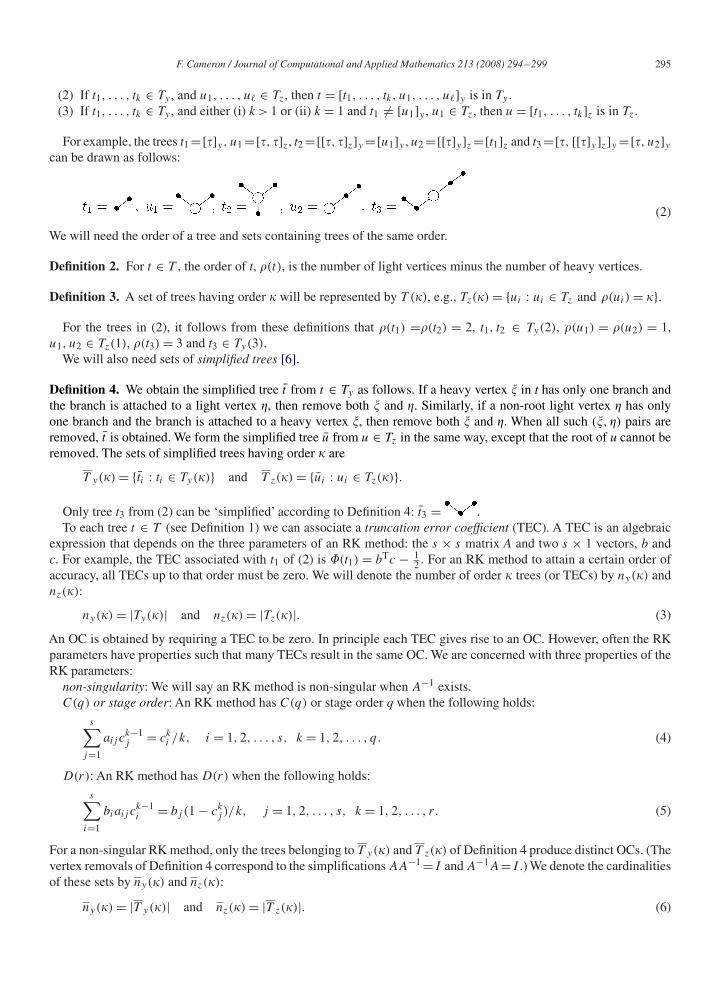
(2) If t1, . . . , tk ∈ Ty , and u1, . . . , u� ∈ Tz, then t = [t1, . . . , tk, u1, . . . , u�]y is in Ty .(3) If t1, . . . , tk ∈ Ty , and either (i) k > 1 or (ii) k = 1 and t1 �= [u1]y , u1 ∈ Tz, then u = [t1, . . . , tk]z is in Tz.

For example, the trees t1 =[�]y, u1 =[�, �]z, t2 =[[�, �]z]y =[u1]y , u2 =[[�]y]z =[t1]z and t3 =[�, [[�]y]z]y =[�, u2]ycan be drawn as follows:

(2)

We will need the order of a tree and sets containing trees of the same order.

Definition 2. For t ∈ T , the order of t, �(t), is the number of light vertices minus the number of heavy vertices.

Definition 3. A set of trees having order � will be represented by T (�), e.g., Tz(�) = {ui : ui ∈ Tz and �(ui) = �}.For the trees in (2), it follows from these definitions that �(t1) =�(t2) = 2, t1, t2 ∈ Ty(2), �(u1) = �(u2) = 1,

u1, u2 ∈ Tz(1), �(t3) = 3 and t3 ∈ Ty(3).We will also need sets of simplified trees [6].

Definition 4. We obtain the simplified tree t from t ∈ Ty as follows. If a heavy vertex � in t has only one branch andthe branch is attached to a light vertex �, then remove both � and �. Similarly, if a non-root light vertex � has onlyone branch and the branch is attached to a heavy vertex �, then remove both � and �. When all such (�, �) pairs areremoved, t is obtained. We form the simplified tree u from u ∈ Tz in the same way, except that the root of u cannot beremoved. The sets of simplified trees having order � are

T y(�) = {ti : ti ∈ Ty(�)} and T z(�) = {ui : ui ∈ Tz(�)}.

Only tree t3 from (2) can be ‘simplified’ according to Definition 4: t3 = .To each tree t ∈ T (see Definition 1) we can associate a truncation error coefficient (TEC). A TEC is an algebraic

expression that depends on the three parameters of an RK method: the s × s matrix A and two s × 1 vectors, b andc. For example, the TEC associated with t1 of (2) is �(t1) = bTc − 1

2 . For an RK method to attain a certain order ofaccuracy, all TECs up to that order must be zero. We will denote the number of order � trees (or TECs) by ny(�) andnz(�):

ny(�) = |Ty(�)| and nz(�) = |Tz(�)|. (3)

An OC is obtained by requiring a TEC to be zero. In principle each TEC gives rise to an OC. However, often the RKparameters have properties such that many TECs result in the same OC. We are concerned with three properties of theRK parameters:

non-singularity: We will say an RK method is non-singular when A−1 exists.C(q) or stage order: An RK method has C(q) or stage order q when the following holds:

s∑j=1

aij ck−1j = ck

i /k, i = 1, 2, . . . , s, k = 1, 2, . . . , q. (4)

D(r): An RK method has D(r) when the following holds:s∑

i=1

biaij ck−1i = bj (1 − ck

j )/k, j = 1, 2, . . . , s, k = 1, 2, . . . , r . (5)

For a non-singular RK method, only the trees belonging to T y(�) and T z(�) of Definition 4 produce distinct OCs. (Thevertex removals of Definition 4 correspond to the simplifications AA−1 =I and A−1A=I .) We denote the cardinalitiesof these sets by ny(�) and nz(�):

ny(�) = |T y(�)| and nz(�) = |T z(�)|. (6)

296 F. Cameron / Journal of Computational and Applied Mathematics 213 (2008) 294–299

Fig. 1. Outline of algorithm for forming sets Ty(�) and Tz(�).

Section 2 contains recursive formulas for ny(�) and nz(�) of (3) and ny(�) and nz(�) of (6). Formulas that take intoaccount C(q) and D(r) are included. We also comment on a class of RK methods lacking the non-singularity property.

2. Recursive enumeration formulas

In what follows, combinations and integer partitions are used. The number of combinations of k items taken from nis C(n, k)= n!/((n − k)!k!) for 0�k�n and C(n, k) = 0 for n < k. Set P� contains the partitions of integer �:

P� = {(j1, j2, . . . , j�) : j1 + 2j2 + · · · + �j� = �, j� �0, j� ∈ Z}. (7)

We will also need the following sets:

�y(�) = {t : t = [u]y, u ∈ Tz(� − 1)}, (8a)

�z(�) = {u : u = [t]z, t ∈ Ty(� + 1)\�y(� + 1)}, (8b)

�y(�) = {t : t = [u]y, u ∈ T z(� − 1)\�z(� − 1)}, (8c)

�z(�) = {u : u = [t]z, t ∈ T y(� + 1)\�y(� + 1)}. (8d)

Considering the trees in (2) we see that t2 ∈ �y(2) and u2 ∈ �z(1).

Total number of trees: We first consider ny(�) and nz(�) from (3). To form a new tree of a certain order, we attachexisting trees—the branches of the new tree—to a new root. To form all new trees we use all possible combinations ofexisting trees. An algorithm for forming Ty(�) and Tz(�) is outlined in Fig. 1. Using this algorithm and (8b) to notethat |�z(�)| = ny(� + 1) − |�y(� + 1)|, we obtain the following enumeration formulas:

ny(�) =∑

(j1,...,j�−1)∈P�−1

�−1∏i=1

C(ny(i) + nz(i) + ji − 1, ji), (9a)

|�z(�)| = ny(�) +∑

(j1,...,j�−1,0)∈P�

�−1∏i=1

C(ny(i) + nz(i) + ji − 1, ji), (9b)

nz(�) = |�z(�)| +∑

(j1,...,j�,0)∈P�+1

�∏i=1

C(ny(i) + ji − 1, ji). (9c)

The partitions given by (j1, . . . , j�, 0) ∈ P�+1 include all members of P�+1 except (0, 0, . . . , 0, 1). The starting valuesfor (9a)–(9c) are ny(1) = 1 and nz(1) = 2.

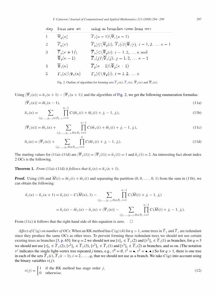
Number of OCs: Next we consider ny(�) and nz(�) from (6). Although sets �y(j) and �z(j) do contain meaningfultrees for forming OCs, it follows from Definition 4 that we should not use trees from these sets as branches whenforming new trees. Taking this into account, an algorithm for forming T y(�) and T z(�) is given in Fig. 2. We will usemy(i) and mz(i) to denote the numbers of trees from T y(i) and T z(i) that can be used as branches:

my(i) = ny(i) − |�y(i)| and mz(i) = nz(i) − |�z(i)|. (10)

F. Cameron / Journal of Computational and Applied Mathematics 213 (2008) 294–299 297

Fig. 2. Outline of algorithm for forming sets T y(�), T z(�), �y(�) and �z(�).

Using |�z(�)| = ny(� + 1) − |�y(� + 1)| and the algorithm of Fig. 2, we get the following enumeration formulas:

|�y(�)| = mz(� − 1), (11a)

ny(�) =∑

(j1,...,j�−1)∈P�−1

�−1∏i=1

C(my(i) + mz(i) + ji − 1, ji), (11b)

|�z(�)| = my(�) +∑

(j1,...,j�−1,0)∈P�

�−1∏i=1

C(my(i) + mz(i) + ji − 1, ji), (11c)

nz(�) = |�z(�)| +∑

(j1,...,j�,0)∈P�+1

�∏i=1

C(my(i) + ji − 1, ji). (11d)

The starting values for (11a)–(11d) are |�y(1)| = |�z(1)| = ny(1) = 1 and nz(1) = 2. An interesting fact about index2 OCs is the following.

Theorem 1. From (11a)–(11d) it follows that nz(�) = ny(� + 1).

Proof. Using (10) and M(i) = my(i) + mz(i) and separating the partition (0, 0, . . . , 0, 1) from the sum in (11b), wecan obtain the following:

nz(�) − ny(� + 1) = nz(�) − C(M(�), 1) −∑

(j1,...,j�−1,0)∈P�

�−1∏i=1

C(M(i) + ji − 1, ji)

= nz(�) − my(�) − nz(�) + |�z(�)| −∑

(j1,...,j�−1,0)∈P�

�−1∏i=1

C(M(i) + ji − 1, ji).

From (11c) it follows that the right-hand side of this equation is zero. �

Affect of C(q) on number of OCs: When an RK method has C(q) (4) for q > 1, some trees in T y and T z are redundantsince they produce the same OCs as other trees. To prevent forming these redundant trees we should not use certainexisting trees as branches [3, p. 65]: for q = 2 we should not use [�]y ∈ T y(2) and [�2]z ∈ T z(1) as branches, for q = 3we should not use [�]y ∈ T y(2), [�2]y ∈ T y(3), [�2]z ∈ T z(1) and [�3]z ∈ T z(2) as branches, and so on. (The notation�j indicates the single light-vertex tree repeated j times, e.g., �0 = ∅, �1 = •, �2 = •, •.) So for q > 1, there is one treein each of the sets T y(i), T z(i − 1), i = 2, . . . , q, that we should not use as a branch. We take C(q) into account usingthe binary variables (j):

(j) ={

1 if the RK method has stage order j,

0 otherwise.(12)

298 F. Cameron / Journal of Computational and Applied Mathematics 213 (2008) 294–299

Table 1Enumeration results for trees and OCs

Item and symbol Order range [�low,�hi] Values

Trees, ny(�) [1, 6] 1, 3, 22, 192, 1972, 22057Trees, nz(�) [1, 6] 2, 13, 112, 1131, 12579, 148963OCs, ny(�) [1, 9] 1, 2, 6, 21, 81, 336, 1466, 6641, 30957OCs, stage order 2, nC

y (�) [1, 9] 1, 1, 2, 5,14, 41, 126, 400,1306OCs, stage order 3, nC

y (�) [1, 9] 1, 1, 1, 2, 5, 13, 35, 96, 269

We set (1) = 0 since the C(1) property does not result in any redundant trees. The enumeration formulas that takeaccount of the C(q) property,

|�C

y (�)| = mCz (� − 1) − (�), (13a)

nCy (�) =

∑(j1,...,j�−1)∈P�−1

�−1∏i=1

C(mCy (i) − (i) + mC

z (i) − (i + 1) + ji − 1, ji), (13b)

|�C

z (�)| = mCy (�) − (�) − (� + 1)

+∑

(j1,...,j�−1,0)∈P�

�−1∏i=1

C(mCy (i) − (i) + mC

z (i) − (i + 1) + ji − 1, ji), (13c)

nCz (�) = |�C

z (�)| +∑

(j1,...,j�,0)∈P�+1

�∏i=1

C(mCy (i) − (i) + ji − 1, ji) (13d)

are modifications of (11). Similarly to my and mz of (10), we have used

mCy (i) = nC

y (i) − |�C

y (i)| and mCz (i) = nC

z (i) − |�C

z (i)|. (14)

Affect of D(r) on number of OCs: Although the C(q) property (4) can be handled by refraining from using certaintrees as branches, the D(r) property (5) cannot. For example, if an RK method does not have D(1) but has C(2), thentree t1 of (2) should not be used as a branch when forming a new tree. However, if an RK method has D(1) but doesnot have C(2), then t1 of (2) must be used as a branch when forming new trees even though, owing to D(1), it does notyield a distinct (non-redundant) OC. So, to handle D(r), we must first use (11) or (13) to count all possible OC treesand then subtract the number of trees made redundant by D(r). There are two cases of redundancy owing to D(r) andboth affect trees in set T y [3, p. 66].

Case 1: For r > 0, the order � trees having the form [�j−1, t0]y , t0 ∈ T y(� − j)\�y(� − j), j = 1, 2, . . . ,

min(r, � − 1) are redundant.

Case 2: For r > 0, the order� trees having the form [�j , u0]y , u0 ∈ T z(� − j − 1)\�z(� − j − 1), j =1, 2, . . . , min(r, � − 2) are redundant.

The number of redundant order � trees owing to D(r) is given by

dDy (�) =

min(r,�−1)∑j=1

mCy (� − j) +

min(r,�−2)∑j=1

mCz (� − j − 1), (15)

where the two summations correspond to cases 1 and 2. To compute the number of OCs taking into accountboth the C(q) and D(r) properties we should proceed as follows: (a) compute nC

y (�), nCz (�), mC

y (�) and mCz (�)

F. Cameron / Journal of Computational and Applied Mathematics 213 (2008) 294–299 299

using (13) and (14), (b) compute dDy (�) from (15) and (c) use

nCDy (�) = nC

y (�) − dDy (�) (16)

to compute the number of OCs for the y-variable.

Number of OCs for a half-explicit method: Brasey and Hairer [1] designed RK methods that lack the non-singularityproperty. For their RK methods the number of order � OCs for the y-variable is given by my(�) of (10). However, thenumber of order � OCs for the y-variable for a second embedded RK method using the same A matrix is ny(�) of (11b).

Some sequences: Table 1 contains values computed from formulas (9), (11) and (13). It is believed that the sequencesin the table are new. These values have been verified by actually generating the trees in Matlab [2].

References

[1] V. Brasey, E. Hairer, Half-explicit Runge–Kutta methods for differential–algebraic systems of index 2, SIAM. J. Numer. Anal. 30 (1994)538–552.

[2] F. Cameron, A Matlab package for automatically generating Runge–Kutta trees, ACM Trans. Math. Software 32 (2006) 274–298.[3] E. Hairer, C. Lubich, M. Roche, The numerical solution of differential–algebraic systems by Runge–Kutta methods, Lecture Notes in Mathematics,

vol. 1409, Springer, Berlin, 1989.[4] E. Hairer, S.P. NZrsett, G. Wanner, Solving Ordinary Differential Equations, vol. I, Nonstiff Problems, Springer, Berlin, 1993.[5] E. Hairer, G. Wanner, Solving Ordinary Differential Equations, vol. II, Stiff and Differential–Algebraic Problems, Springer, Berlin, 1996.[6] A. KværnZ, Runge–Kutta methods applied to fully implicit differential–algebraic equations of index 1, Math. Comput. 54 (1990) 583–625.