1

Entry and Pricing in a Differentiated Products Industry: Evidence from the ATM Market

Gautam Gowrisankaran University of Arizona, HEC Montreal and NBER

gautamg2@gmail.com

John Krainer Federal Reserve Bank of San Francisco

john.krainer@sf.frb.org

This version: January, 2011

Abstract: We estimate a structural equilibrium model of the automatic teller machine market (ATM) to evaluate the implications of regulating ATM surcharges. We use data on bank characteristics, potential and actual ATM locations, and consumer locations; identify the model parameters with a regression discontinuity design; and develop methods to estimate the model without computing equilibria. A surcharge ban reduces ATM entry 12 percent and consumer welfare 24 percent but increases firm profits 27 percent. Total welfare under either regime is 4 percent lower than the surplus maximizing level. The paper can help shed light on the implications of unregulated entry for differentiated products industries. We thank Dan Ackerberg, Steve Berry, Jeremy Fox, Phil Haile, Fumiko Hayashi, Igal Hendel, Kei Hirano, Tom Holmes, anonymous referees, and seminar participants at numerous institutions for helpful comments, Joy Lin, Yuanfang Lin, and Chishen Wei for research assistance and Anita Todd for editorial assistance. Gowrisankaran gratefully acknowledges financial support from the National Science Foundation (Grant SES-0318170), the NET Institute, and the Federal Reserve Bank of New York. The views expressed in this paper are solely those of the authors and do not represent those of the Federal Reserve Banks of New York or San Francisco or the Federal Reserve System. An earlier version of this paper was distributed under the title “The Welfare Consequences of ATM Surcharges: Evidence from a Structural Entry Model.”

2

1. Introduction

The goal of this paper is to estimate a structural equilibrium model of the market for

automatic teller machines (ATMs) and use the model to understand the implications of

regulating ATM surcharges on entry, pricing, and welfare. We develop econometric methods to

feasibly estimate the parameters of the model without computing equilibria. Our estimator uses

ATM entry data and also the fact that surcharges were banned in Iowa but not in neighboring

Minnesota. We develop conditions under which our structural model of differentiated products

demand is identified using entry data but not price or quantity information. This paper can help

shed light on the theoretically ambiguous implications of free entry for consumer and producer

welfare for differentiated products industries in general, and ATMs in particular.

Since the establishment of the first ATM networks in the early 1970s, ATMs have

become a ubiquitous and growing component of consumer banking technology. By 2001, there

were over 324,000 ATMs in the United States, processing an average of 117 transactions per

ATM per day, suggesting that each person in the United States uses an ATM an average of 45

times per year (ATM & Debit News, 2001). In spite of the ubiquity of ATMs, product

differentiation implies that the market for ATMs may not reflect perfect competition or yield

optimal outcomes. In particular, the surcharge—the price charged by an ATM on top of the set

interchange fee—has increased significantly over time. The increase can be linked to an April

1996 decision by the major ATM networks to allow surcharges among their member ATMs.i

Between 1996 and 2001, the number of ATMs tripled, but the number of transactions per ATM

fell by about 45 percent (McAndrews, 1998).

The technology of ATMs is characterized by high fixed costs—primarily the cost of

leasing the machine, keeping it stocked with cash, and servicing it—and very low marginal costs.

3

Thus, the increased price of ATM services has been accompanied by an increased average cost

per ATM transaction. The increase in price suggests that there may have been “excess” entry of

ATMs, in the sense that total welfare would have been higher with less entry. It also suggests

that a policy by an ATM network or government that regulated or eliminated surcharges could

potentially increase total welfare. This would likely be true if new ATMs stole significant

business from existing ATMs without sufficiently adding to consumer welfare. However, ATMs

are differentiated products, with a primary characteristic being their location. The increase in the

number of ATMs implies that consumers have to travel less distance to use an ATM. This

decrease in distance can compensate for the increase in price. Therefore, it is theoretically

ambiguous whether price restrictions would increase or decrease welfare. The answer depends

on the relative weight of price and distance in the consumer utility function, firm cost structures,

and the nature of the equilibrium interactions between agents in the economy.

We address these questions by specifying a static discrete choice differentiated products

model of the ATM market in a rural county. In our model, banks and nonbanks (generally

grocery stores), simultaneously decide whether to install ATMs. Banks have branches and an

associated set of depositors. Banks benefit in two ways from opening an ATM: lower costs from

depositors using an ATM instead of a teller, and interchange fees and surcharges collected from

nondepositors. Banks do not surcharge their own depositors for using their ATM. Nonbanks do

not have depositors and, hence, open ATMs solely to collect interchange fees and surcharges.

Consumer utility for an ATM is a function of distance and price, but as is common in discrete

choice models without quantity data (e.g., Thomadsen, 2005), utility is not a function of any

unobserved location characteristics due to the difficulty in identifying both utility and cost

shocks with limited data. Firms face a fixed cost per ATM that can vary by location, but no

4

marginal costs. Entry decisions and prices are determined in a simultaneous–moves Nash

equilibrium. We create a dataset that merges bank characteristics with actual and potential ATM

locations for the border counties of Iowa and Minnesota, estimate the structural parameters of the

model, and use our estimated parameters to assess the equilibrium implications of a surcharge

ban and other policies.

In general, it might be difficult to identify cost and preference parameters using only

entry data. However, we are able to identify and estimate these parameters by using the fact that

the state of Iowa banned ATM surcharges during our sample period.ii We show that the fixed

prices in Iowa, together with our observation of potential and actual ATM locations, identify the

distance disutility, firm cost, and consumer utility parameters. The ban on surcharges in Iowa but

not its neighboring states creates a regression discontinuity design (RDD), whereby the different

pattern of ATM penetration rates between places in Iowa near its borders and places just outside

the borders of Iowa identify the price elasticity of demand.iii Intuitively, more inelastic demand

will imply that firms in Minnesota can earn higher profits from entry, and hence that entry rates

in Minnesota will be higher relative to Iowa. We believe that a contribution of the paper is to

develop ways to identify equilibrium industry models with data on entry decisions under

different policy regimes.

This study builds on an entry literature started by Bresnahan and Reiss (1991) and Berry

(1992). Like more recent papers in this literature (Chernew, Gowrisankaran, and Fendrick

(2002), Mazzeo (2002), and Seim (2006)), we incorporate detailed geographic and product data

that allow us to obtain more realistic results. Our model is methodologically most similar to Seim

(2006). As in that paper, we assume that firms operating within a market have incomplete

information, in that they do not know their competitors’ cost shocks. We also specify the precise

5

location of potential firm entry points within a localized area. A model of localized competition

is crucial for understanding the welfare impact of ATM surcharges because of the consumers’

tradeoff between location and price.

Our contribution to this literature is to model fundamental utility parameters and develop

conditions under which our data identify these parameters. We also develop econometric

methods that allow us to estimate the parameters without solving for the equilibria of the game,

thereby reducing the computational burden of estimating the model. Here, our methods apply

techniques developed for other contexts by Aguirregabiria and Mira (2007), Bajari, Benkard and

Levin (2007), Guerre, Perrigne, and Vuong (2000), Hotz and Miller (1993) and Pakes,

Ostrovsky, and Berry (2007).

A recent literature on ATM surcharges (Croft and Spencer (2003), Hannan, Kiser,

McAndrews, and Prager (2004), Ishii (2005), Knittel and Stango (2004), and Massoud and

Bernhardt (2002)) also bears on this work. Most of the papers in the literature model price and

quantity under alternate regimes. Our approach builds on this literature in terms of the richness

of the consumer specification (which notably includes distance), RDD source of identification,

and equilibrium nature of our model. In particular, an equilibrium model is necessary to

understand the impact of counterfactual policies. We are aware of only one other estimated

equilibrium ATM model, Ferrari, Verboven, and Degryse (2009), which is applied to Belgian

data. Our model of banks builds on this paper in that we similarly specify banks as depository

institutions. However, we specify oligopoly (rather than monopoly) interactions and allow for

distance, rather than the number of ATMs in a county, to influence utility.

The remainder of this paper is divided as follows. Section 2 details the data, including

background on the industry and some reduced–form evidence. Section 3 describes the model and

6

inference. Section 4 provides the results of the estimation and the policy experiments, including

Monte Carlo evidence on the performance of our estimator. Section 5 concludes.

2. Industry and data

The ATM industry

The ATM industry infrastructure consists of card–issuing banks, ATM machines, and a

telecommunications network to process transactions.iv In the early stages of ATM deployment,

ATMs were generally owned and operated by banks, with the machines physically located on the

bank premises. The ATM technology was attractive to banks as a means of shifting routine

customer transactions, such as cash withdrawals, away from relatively costly bank tellers. By the

1990s, much of the growth in ATM deployment shifted to nonbank locations, such as

convenience stores and grocery stores (McAndrews, 1998). Today, the majority of ATMs are

located at sites other than banks. More than 75 percent of all ATM transactions are cash

withdrawals, with the remainder being deposits and balance inquiries.

ATM cardholding consumers, ATMs, and card–issuing banks are all linked together by

shared networks. In 2002, there were about 40 networks, the largest being the national networks

of Cirrus and Plus, owned by MasterCard and Visa, respectively (Hayashi, Sullivan, and Weiner,

2003). A transaction involving a depositor from Bank A using an ATM owned by Institution B

generates a number of fees. Bank A must pay the network a switch fee for routing the

transaction. These fees range from 3 to 8 cents per transaction. In the following analysis we do

not model the switch fee. Second, Bank A, the card–issuing bank, must pay Institution B an

interchange fee. These fees range from 30 to 40 cents for a withdrawal and are determined by the

7

ATM network. In the case where an ATM and a consumer’s bank both use multiple networks,

the actual interchange fee will vary based on the agreements between the ATM and the different

networks. In our estimation, we approximate the interchange fee, pinterchange as 35 cents.

Bank A may also charge its own depositor a foreign fee for using Institution B’s machine.

Our analysis does not consider this fee. Institution B may charge the consumer a surcharge fee

for using its ATM machine. As of 2002, 87 percent of all ATM deployers levied surcharges on

foreign-acquired consumers. The average surcharge across all operators was about $1.00

(McAndrews, 1998). Fees are typically paid by only about one-third of consumers (Dove

Consulting, 2002), as consumers do not pay fees to ATMs of their own bank.

According to a recent consulting study, the average ATM cost $1,314 per month to

operate in 2003, with the costs consisting mostly of fixed items such as depreciation,

maintenance, telecommunications, and cash replenishment (Dove Consulting, 2004).

Sample and data

We define a market to be a rural county. As our model is identified by the difference in

the pattern of ATM diffusion for Iowa and Minnesota, we want the Iowa and Minnesota counties

in our sample to be similar in terms of consumer preferences and firm costs. To ensure similarity,

we focus on the border counties from each state as well as counties that are within one county of

the border. Eight of the counties in the eastern part of Minnesota have more population density

than the corresponding Iowa counties and include medium-sized cities such as Rochester. We

believe that the dense counties are sufficiently different from the corresponding Iowa counties,

and so we exclude these counties from our sample. Figure 1 displays a map of the counties in our

sample and their population densities.

8

Our choice to study sparsely populated rural counties limits our ability to generalize the

results to different market structures. In particular, because of higher population densities, urban

markets are likely to have many more equilibrium ATMs per square kilometer, suggesting that

the benefits from allowing surcharges are more limited. However, the disutility from distance

traveled may also be higher in urban markets, due to higher travel times per kilometer,

suggesting that a greater density of ATMs is needed to achieve the same welfare level. Although

these two effects have opposite implications regarding the benefits of allowing surcharging, our

prior is that the additional entry from surcharges will reduce equilibrium travel times the most in

rural markets, implying that rural markets would likely have a greater gain from allowing

surcharges than would other markets.

To implement our analysis we require data on potential ATM locations, actual ATM

entry, consumer locations, and bank deposits. Our data come from the year 2002, prior to the

lifting of the surcharge ban in Iowa.v We discuss each of these data sources in turn.

Our first dataset provides the set of potential ATM locations. ATMs are almost certain to

be located inside other retail establishments, particularly in the rural counties from our sample.

To attempt to narrow down the set of possible locations, we obtained phone numbers for all the

retail establishments in one county in Iowa (Mitchell County).vi By calling every retail

establishment in that county and asking if there was an ATM on the premises, we found that the

ATMs were all located in either grocery stores (including convenience stores) or banks. Based

on this initial query, we chose grocery stores and banks as the set of potential ATMs. We

obtained the addresses and phone numbers of grocery stores and banks for our counties from a

private company called InfoUSA, which markets this information for commercial use. We then

9

geocoded these addresses to obtain detailed latitude and longitude information, which we used to

compute distance.

Given a set of potential ATM locations, our second data source contains information on

the locations of actual ATMs that entered the market. We obtained location data from several

large ATM networks with substantial operations in Minnesota and Iowa. The networks in our

dataset include Visa Plus, a network that is national in scope, and SHAZAM, a regional network

based in Iowa that has ATMs throughout the central states.vii These data provide the addresses of

ATMs for all machines in the databases of the networks. After some investigation, we found that

these lists were not complete and hence we called every InfoUSA potential entrant (i.e., grocery

stores, and banks) in our sample and asked if there was an ATM on the premises. For Iowa, this

process identified an additional 93 entrants (24 percent of the total number of entrants). For

Minnesota, we identified an additional 105 entrants from the telephone interviews (52 percent of

the total).

We also found a relatively small number of ATMs in the ATM location data that were

not in the InfoUSA potential ATM dataset. Upon closer inspection (in many cases, we called the

establishment at that location), we learned that these missing potential ATMs actually existed

and were distributed fairly evenly across the counties in our sample, accounting for about 10

percent of the total potential ATMs in each state. We added these ATMs to the list of potential

ATMs. Also in this process we found 9 ATMs in specialized categories, such as colleges,

hospitals, and car washes. We opted to include these observations to the potential ATM data.

Given the relatively low incidence of nonbank and non-grocery store ATMs in our data, we

believe that any misspecification of the set of potential ATM location sites arising from our

focus on banks and grocers will be fairly minor.

10

We obtained population counts and locations for the consumers in our markets from the

1990 Census. The consumer locations are the geographic coordinates of the centroid of each

census block. This level of geographic detail is not quite as fine as the address level but is still

very small. It would be possible to supplement these data with data on employment locations,

treating these locations as additional people, although this would likely have little effect because

of the similarity of residential and employment locations in our sample of rural counties.

Finally, our banking data come from two sources. First, we used data from the 2002

Summary of Deposits (SOD) collected by the Federal Deposit Insurance Corporation (FDIC),

which contains annual records of all branch locations and the deposits booked in those branches.

The set of reporting institutions includes all FDIC-insured depository institutions, including

commercial banks, savings banks, and thrifts but not credit unions. In our potential ATM

locations file we found 19 ATMs located at credit unions. For the purposes of this analysis we

consider banks and credit unions as “banks” in the sense that they take in deposits and may have

similar incentives to banks for establishing ATMs. Second, we obtained consolidated (not

branch-level) deposits for credit unions from the National Credit Union Administration’s 5300

Report. Fortunately, the credit unions in our sample tend to be very small, single-branch

institutions, so that branch deposits are the same as consolidated balance sheet deposits. Our data

contain four multi-branch credit unions for which we assign each branch an equal share of the

parent’s total reported 2002 deposits.

We merged the bank and credit union deposit data with bank potential ATM entrant data

using the address field to obtain the customer base of each bank. In 9 cases, we found no deposit

record of the bank in the deposit data and no ATM and hence we deleted the bank from the set of

11

potential entrants; in 24 cases, we found deposit data but no record of the ATM in the potential

entrant data. We added these banks to the list of potential ATMs.

For some of our estimates, we allow the entire border region to have the same mean fixed

costs for ATMs. For other estimates, we allow the mean fixed costs to vary across counties. For

these estimates, we group the mean fixed costs so that the Iowa border county, its southern

neighbor (e.g., Lyon and Sioux, respectively) and its closest Minnesota neighbors (Pipestone and

Rock, in this case) all share the same fixed costs.

Summary statistics and reduced-form evidence

Table 1 provides some summary statistics of the data. The table generally supports our

notion that the Iowa and Minnesota border counties are quite similar in terms of population

density and banking structure, while differing somewhat in terms of the profile of ATM

deployment. We have 32 counties in our data, of which 21 are in Iowa. Our counties are sparsely

populated, with an average of about 16,000 people per county in Iowa and somewhat fewer in

Minnesota. In spite of the relatively small populations in this region of the country, each county

contains about 1,000 census blocks, suggesting that the unit of geographic measurement for

people is small.

The banking market structures in the Iowa and Minnesota counties are also roughly

similar. On average, there are 8 banking firms per county in Iowa, versus 9.2 firms in Minnesota.

The banking markets in both the Iowa and Minnesota counties are unconcentrated.1

On average there are about 14 percent fewer potential ATM locations in Minnesota than

in Iowa. The number of potential ATMs varies quite a bit across counties; in Iowa, varying from

a low of 14 to a high of 86. In Iowa, there are an average of 18.8 ATMs per county and 1.13

12

ATMs per 1,000 people. The corresponding statistics for Minnesota are 18.3 and 1.23,

suggesting that the unregulated price may result in more entry. We define a potential ATM site

to be a “bank” location if the site is located on bank or credit union premises.viii Bank entry rates

(i.e., bank ATMs as a percent of potential bank ATMs) are, on average, higher than nonbank

entry rates in Iowa, while the opposite is true in Minnesota where surcharges are permitted.

We can sharpen this intuition about the differences in ATM entry patterns across the two

states with a county-level regression of ATMs per person on a state dummy variable, including

controls for the number of consumers and potential entry locations, shown in Table 2. Table 2

reports that Iowa counties have about .2 ATMs per thousand fewer than the Minnesota counties

with similar characteristics. This estimated difference is somewhat larger than is observed in the

raw data in Table 1, and is explained by the fact that the Iowa counties have more potential ATM

locations, which is associated with more entry.

In addition to predicting more entry in Minnesota because of the ability to surcharge, we

also might expect a different pattern of entry. In particular, entrants in Minnesota should be more

likely to stay away from other potential entrants, in order to exercise more local monopoly

power. The last row of Table 2 examines whether this prediction is substantiated in the data. We

find limited evidence consistent with this hypothesis: ATMs in Iowa are more likely to be near

other potential ATMs, but the effect is not significant.

3. Model and Inference

Model

13

We develop a simple game–theoretic model of the ATM market that we estimate using

data on bank characteristics, consumer location, and actual and potential ATM locations. Our

model is static, which we believe to be a reasonable approximation because sunk costs in the

ATM industry are low: machines can be resold, and ATMs are generally installed within existing

retail establishments.

We consider a market to be a rural county. All econometric unobservables are i.i.d. across

markets. The unit of observation is the set of all firms that can plausibly install ATMs in the

county, which we label j= 1,…,J . Each firm is either a bank or a nonbank; nonbanks are

generally small grocery or convenience stores.

We model several differences between nonbanks and banks. Nonbanks operate ATMs

solely to maximize the profits from interchange fees and surcharges obtained from consumers

withdrawing cash. Each nonbank location is owned by an individual entrepreneur. We make the

assumption of individual ownership because we believe that it is the norm for convenience stores

in rural areas and because we lack ownership data for nonbanks.

In contrast to nonbanks, banks have depositors that are associated with them. Banks

provide their depositors with teller services for withdrawals and deposits, and sometimes, with

ATMs. Banks do not surcharge their own depositors when they use their own ATMs, and they

must pay the interchange fees when their depositors use other ATMs. In some specifications,

banks can have multiple branches in a market. Let o j( ) denote the number of branches and let

j1,…, j

o j( ) denote the set of branches owned by bank j. In addition to the profit motives of

nonbanks, banks may open ATMs to reduce the use of teller services and interchange fees paid

on behalf of their depositors.

14

We assume that the marginal cost of an ATM transaction is zero. We make this

assumption because, except in very crowded locations where there is queuing and hence a

shadow cost of ATM usage, the marginal cost of using an ATM is trivial, consisting roughly of

the small amount of ink and paper used to print a receipt. We assume that fixed costs are

F

jk

= FC ! "ee

jk

where FC are the mean fixed costs, e

jk

is a fixed cost shock and e

! is a

parameter to estimate. As discussed in Section 2, we allow FC to vary across groups of markets

in some of our specifications.

In Minnesota, where surcharging is permitted, each firm first chooses its price

(conditional on entry). For tractability, we assume that each multi-branch firm is constrained to

choose the same price for all of its branches in a market. Let the price be p

j. In Iowa, prices are

set to 0 by law.

Following the choice of price, firms obtain the realization of their e

j cost shocks. We

assume that each e

j is distributed as the difference between two i.i.d. Type 1 extreme value

random variables. Each firm observes the shocks for all of its branches, and then simultaneously

decides at which of its branches to install an ATM.ix The shocks are known only to the firm and

not to competitors. Unobservable cost shocks of this type have recently been used in a number of

applications in the entry literature (see, for instance, Seim, 2002; Augereau, Greenstein and

Rysman, 2002; and Bajari, Hong, Krainer and Nekipelov, 2010), as they help reduce the number

of equilibria for entry models. One drawback of this assumption is that firms that enter may

sometimes suffer ex-post regret.

We now describe the consumer decision problem. Consumers are differentiated on two

observable dimensions: their geographic location and their bank. Let kjx denote the deposit

15

share for branch k of bank j in the market. Denote consumer locations i = 1,…, I and let

iM

denote the number of consumers at location i. We assume that each bank branch’s share of

depositors at each location i is proportional to their banking deposits in the market.x Consumers

observe the set of actual ATMs and banks as well as the surcharge (equivalently, price) for each

ATM. In Iowa, these prices are fixed at zero, although the interchange fee that the ATM receives

from the transaction is positive.

Having observed the prices, each consumer must make a discrete choice for her cash

withdrawal services from among (a) the branches of her own bank (whether or not they have

ATMs), (b) ATMs not at her bank, and (c) the outside option. The outside option, which is to not

obtain cash, has u

i0= !

c"

i0 where

0i! is an idiosyncratic unobservable.xi Since depositors will

not be charged a price for transactions at any teller or ATM branch of their bank, the utility for a

depositor i of bank j making a withdrawal transaction at any branch k of her own bank is

(1) u

ijk

= ! + "dij

k

+ #c$

ijk

,

where d

ijk

is the distance from consumer i’s location to the location of branch k of bank j, δ is

the gross mean benefit from using the ATM, α is a parameter that indicates the impact of

distance on utility and !

ijk

is again an idiosyncratic unobservable. For a depositor i of bank h,

h j! , making a withdrawal at an ATM at location k of firm j, the utility is

u

ijk

= ! + "dij

k

+ #pj+ $

c%

ijk

where β is a parameter that indicates the price sensitivity. As is

generally true in discrete choice models, we cannot identify !

c. Hence, we exclude

!

c when

16

estimating equation (1). The other parameters in the consumer utility function should be

interpreted as their true values divided by !

c.

We assume that upon choosing to withdraw cash at a branch owned by their home

institution, consumers will choose the ATM if it exists and otherwise will choose the teller.

Equivalently, the utility of an ATM is very slightly higher than that of a co-located teller and

they have the same ε draws.

We assume that !

ijk

is distributed Type I extreme value, which gives rise to a

multinomial logit expected quantity formula. Let y

jk

be a 0–1 indicator for whether firm j has

opened an ATM at location k, and define s

ijk

h yJ ,pJ( ) to be the expected share for branch k of

firm j, for a consumer at location i who is a depositor at bank h, faced with an entry vector yJ

and a price vector pJ . Then, we obtain:

(2)

sij

k

h yJ ,pJ( ) =1 j= h or y

jk

= 1{ }exp ! + "dij

k

+1 j# h{ }$pj( )

1+ 1 m = h or ym

n

= 1{ }exp ! + "dim

n

+1 m # h{ }$pm( )

n=1

o m( )

%m=1

J

%

,

where the term 1 j= h or y

jk

= 1{ } occurs because potential ATM location of bank j can always

be used by depositors of bank j and can otherwise only be used if the firm has opened an ATM.

We now specify two avoided costs from ATM entry. Let w! denote the marginal cost of

a teller transaction. By opening an ATM, the bank obtains a cost savings of !

w for each of its

depositors that use their own bank for withdrawals. In addition to cash withdrawal, some fraction

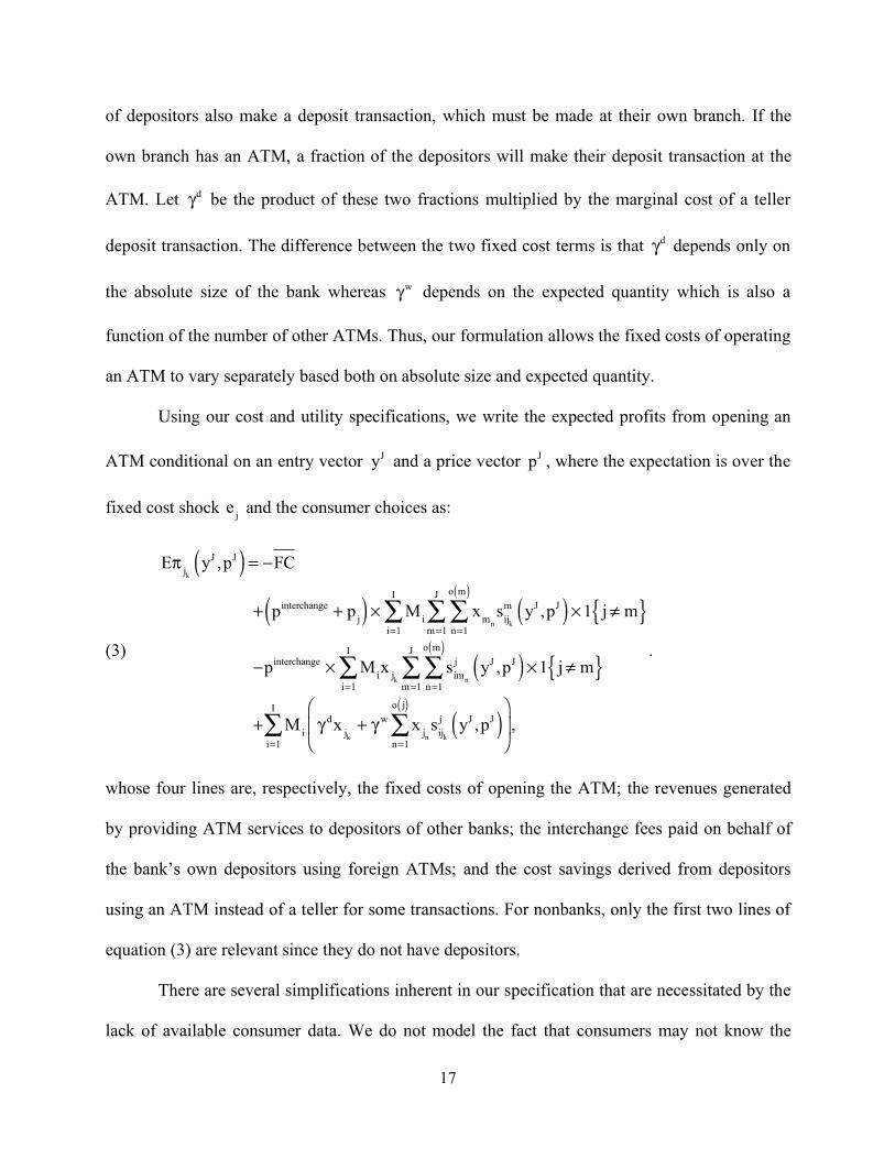
17

of depositors also make a deposit transaction, which must be made at their own branch. If the

own branch has an ATM, a fraction of the depositors will make their deposit transaction at the

ATM. Let d! be the product of these two fractions multiplied by the marginal cost of a teller

deposit transaction. The difference between the two fixed cost terms is that d! depends only on

the absolute size of the bank whereas w! depends on the expected quantity which is also a

function of the number of other ATMs. Thus, our formulation allows the fixed costs of operating

an ATM to vary separately based both on absolute size and expected quantity.

Using our cost and utility specifications, we write the expected profits from opening an

ATM conditional on an entry vector yJ and a price vector p

J , where the expectation is over the

fixed cost shock e

j and the consumer choices as:

(3)

E!jk

yJ ,pJ( ) = "FC

+ pinterchange+ p

j( ) # Mi

xm

n

sij

k

m yJ ,pJ( ) #1 j$ m{ }n=1

o m( )

%m=1

J

%i=1

I

%

"pinterchange # Mix

jk

sim

n

j yJ ,pJ( ) #1 j$ m{ }n=1

o m( )

%m=1

J

%i=1

I

%

+ Mi& dx

jk

+ & w xjn

sij

k

j yJ ,pJ( )n=1

o j( )

%'

()

*

+,

i=1

I

% ,

.

whose four lines are, respectively, the fixed costs of opening the ATM; the revenues generated

by providing ATM services to depositors of other banks; the interchange fees paid on behalf of

the bank’s own depositors using foreign ATMs; and the cost savings derived from depositors

using an ATM instead of a teller for some transactions. For nonbanks, only the first two lines of

equation (3) are relevant since they do not have depositors.

There are several simplifications inherent in our specification that are necessitated by the

lack of available consumer data. We do not model the fact that consumers may not know the

18

prices or locations of all ATMs, and hence that there may be a search cost in addition to travel

costs. Banks cannot attract depositors by adding more ATMs. We do not allow banks to charge

their own depositors foreign fees when they use another bank’s ATM. We assume that bank

tellers are always open. Despite these simplifications, our model does capture the key factors that

differentiate a bank’s incentives to install an ATM from a nonbank’s incentives. Namely, the

model allows banks to price discriminate by not surcharging their own depositors, and to install

ATMs as a way of lowering the costs of their banking services.xii

Because of the incomplete information about the cost shocks, we use a Bayesian–Nash

equilibrium (BNE) concept. A BNE specifies, for each firm j, a price p

j, and a mapping from the

vector of fixed cost shocks for its branches je , to its entry vector jy . Since entry configurations

by rival firms enter into profits in equation (3), the optimization conditions can be expressed in

terms of the entry density of rivals. Formally, let f

jy

j( ) denote a density of entry configurations

for firm j and let f! j

y! j( ) denote the analogous product of densities for the competitors of firm j.

Given any f! j

y! j( ) , the BNE entry decisions must satisfy

(4)

yj

ej,pJ( ) f! j

y! j( ) = arg maxy

j1,…, y

jo j( )

Ey! j

E"jk

yj1

,…, yjo j( )

, y! j,pJ#

$%& + '

ee

jk

#$(

%&)

k=1

o j( )

* ,

for each firm j, where E

y! j

is the expectation with respect to y! j

.

In Iowa, equation (4) is evaluated at pJ= 0 . In Minnesota, since each firm is a Bertrand

competitor, each firm chooses price together with an entry strategy. The BNE condition for price

in Minnesota is thus

19

(5)

pj= arg max

pj

EyJ

E!jk

yJ , pj,p

" j( )k=1

o j( )

#$

%&&

'

())

*+,

-,

./,

0,,

which jointly with (4) must hold simultaneously for each firm j.

Identification

Our data are quite different from the data commonly used to identify consumer

preferences for discrete choice utility specifications. Principally, we lack data on prices (except

for the interchange fees) and quantities. In spite of this, and although our base model is fully

parametric, we can show that the model is semi-parametrically identified in the sense that

identification does not depend on parametric assumptions about the cost density. We allow fixed

costs jF to have an unknown distribution function G !( ) with accompanying density function

g !( ) . We assume this density to be the same across firms and counties.

We first explain identification informally using a simplified version of our model, where

prices are 0 (as in Iowa), all consumers and firms are located at the same place, and all potential

entrants are nonbanks. In this case, if we had data (that do not exist) on potential quantities given

entry, consumer utility δ would be identified as in standard discrete choice models. Moreover,

potential quantity multiplied by pinterchange yields marginal profits, and hence the probability of

entry given any level of marginal profits identifies one point of the fixed cost distribution. By

varying potential quantity, one can trace out the whole fixed cost distribution non-parametrically,

even conditioning on the number of potential entrants. Lacking any data on quantities, we can

still identify fixed costs if we know δ. Thus, the challenge is to identify δ. This parameter is

identified by the extent to which additional potential entrants translate into additional actual

20

entrants. With very low values of δ, a new entrant draws all its consumers from people who

would have chosen the outside good. Hence, having additional potential entrants does not affect

the probability of any potential entrant entering. For higher values of δ, new entrants steal more

and more business from existing firms and hence the probability of any one potential entrant

entering drops with additional potential entrants. The price coefficient is then identified from the

difference in entry rates between Iowa and Minnesota counties. Identification of the other terms

on distance and bank teller costs is also straightforward.

In order to formalize the identification of our model, we require a number of regularity

assumptions:

Assumption 1:

(a) Let the support of G be compact and known. Let ( )G 0 0= so that fixed costs are always non-

negative and let ( )g x 0> when ( )0 G x 1< < so that there are no mass points.

(b) Let all parameters of the model lie within compact, known sets.

(c) Letting I and J denote the maximum number of consumers and firms, respectively, assume

that J ! 2 and I is sufficiently large such that for the lowest δ (which is defined by part (b)),

two firms which both draw the lowest e and who each have a market of I consumers located at

zero distance from them will always enter.

(d) For some d 0> , let the density of all consumer and producer locations and bank deposits

have positive mass for all cases for which I ! I , { }J 1,2! and all distances are less than d .

(e) The same equilibrium is played across different markets with identical observables and the

realized equilibrium actions are continuous in market observables.

21

Note that Assumption 1(c) specifies a continuous density for consumers even though in reality

there are integer numbers of consumers at any location. Given the large number of consumers

typically residing in a county, we do not believe that this is a very significant deviation.

To prove identification, we assume that the joint data density is known and show that this

allows for the recovery of the structural parameters and distributions. To simplify the exposition,

we consider again a stripped-down version of the model where there are only nonbanks. Adding

banks complicates the derivations but does not otherwise result in any problems for proving

identification.xiii

Let E y I,J,State( ) denote the entry probability (equivalently, the conditional expectation

of y) that a nonbank enters given that there are I consumers and J entrants, all nonbanks, all

located at the same location in a county in State, where State ! IA,MN{ } . These conditional

probabilities exist by Assumptions 1(c) and (e).

Consider the one- and two-firm probabilities, E y I,J = 1,IA( ) and

E y I,J = 2,IA( ) for

all I ! I and a fixed δ, ! . Using just these probabilities, for each J, we can recover a fixed cost

density under the hypothesis that ! = ! . Let G

J,!e( ) denote the recovered fixed cost density for

a given J. Recovering G

1,!e( ) is straightforward: marginal expected profits conditional on entry

and J = 1 are

(6) !

" ,1,I= I

exp "( )1+exp( "( )

pinterchange ,

where !

" ,J ,I are the marginal expected profits with ! , I consumers and J firms. Hence

22

(7) G

1,!I

exp !( )1+exp( !( )

pinterchange( ) = E y I,J, IA( ) .

By Assumptions 1(a) and (c) and the continuity of equation (6) in I, the value inside the

parentheses on the left side of equation (7) will take on all values in the support of G. It is more

difficult to derive G

2,!e( ) since the expected marginal profits, which depend on the Bayesian

Nash equilibrium of the 2-firm industry, are more complicated than (6). However, it remains true

that for a given ! and J, the marginal profits from the Bayesian Nash equilibrium are 0 when

0I = , continuously increasing in I, and sufficient to generate entry always when I is sufficiently

large. Thus, using E y I,J = 2,IA( ) we can recover

G

2,!e( ) .

Note that, since the true fixed costs density is i.i.d., G

1,!0

e( ) = G2,!

0

e( ) , at the true 0

! . As

discussed above, different values of ! imply different substitution patterns from the outside

good to an ATM as N increases from 1 to 2. Intuitively, marginal profits for J = 2 relative to

J = 1 will be decreasing as ! increases, or for a given set of entry probabilities E y I,J = 1,IA( )

and E y I,J = 2,IA( ) , recovered fixed costs will be decreasing for J = 2 relative to J = 1 as !

increases. Only at 0

! = ! will the fixed cost distributions be equal. Formally,

Lemma 1: 01, 2,

G G! != " ! = ! .

Proof: See appendix.

This leads directly to our main result:

Proposition 1: The Iowa data E y I,J = 1,IA( ) and

E y I,J = 2,IA( ) for all I ! I semi-

parametrically identify δ and G !( ) .

23

Proof: The identified values are the unique 0

! for which 0 01, 2,

G G! != and the accompanying

01,G

! density. •

The Iowa data will also identify the other parameters except for the price coefficient. To

identify the distance parameter α, we consider the conditional probability of entry when there are

I consumers, J = 1 firms and all consumers are located at the same place, but that location is at

distance d from the firm location, where, 0 < d < d . Such markets exist by Assumption 1(d).

Marginal profits are then ( )

( )0

0

exp d interchange

1 exp( dI p

! "#

+ ! "#, implying that the entry probability is lower the

higher is α. The identified α is the one that fits the entry probability for this type of market.

Identification of the teller cost parameters d! and w

! , also follow from Assumption 1(d). The

deposit parameter d! will be identified by the extra entry probability of banks relative to

nonbanks as the market size increases, holding shares constant. The withdrawal parameter, w!

will be identified by the extra entry probability of banks relative to nonbanks as their deposit

share increases, holding market size constant.

The Minnesota data are necessary to identify the price coefficient. By assumption, every

parameter except the price coefficient β is known when approaching these data. Intuitively, a

more negative β leads to lower equilibrium prices and hence less entry. The true β is the unique

one that matches the Minnesota entry rates. Formally, consider again a market with one firm and

no location differences and some I for which 0 < E y I,J,MN( ) < 1 . The firm will enter when:

(8) max

pI

exp !+"p( )1+exp( !+"p( )

p + pinterchange( ) # FC > 0{ } .

Letting *p denote the price that solves (8), the probability of entry for this β is then

24

(9)

E !y !( )( ) = G Iexp "+!p*( )

1+exp( "+!p*( )p*

+ pinterchange( )#$%

&'(

.

Using the envelope theorem to hold p constant at *p when differentiating profits, we obtain

(10)

dE !y !( )( )d!

= p*g Iexp "+!p*( )

1+exp( "+!p*( )p*

+ pinterchange( )#$%

&'(

Iexp "+!p*( )

1+exp( "+!p*( )( )2

p*+ pinterchange( ) .

By Assumption 1(a), this derivative is strictly positive provided price is positive. The identified

value of β is the unique one that sets E !y !( )( ) = E y I,J,MN( ) .

Note that we have only used data from markets with one distance level to identify the

distance coefficient and data from markets with one firm to identify the price coefficient. In

principle, we could identify more general specifications using data with different distance levels

and firms.

Estimation

Group together the structural parameters as ! = ",#,$,% d

,% w,&

e( ) , denote the true

parameters 0

! , let jz denote the exogenous data for the firm j, which includes consumer

locations, bank locations and deposit amounts and the surcharge regime (i.e., IA or MN), and let

z

J= z

1,…,z

J( ) . While the model description considered one county–market, we now allow

multiple markets. Given that our model is identified under Assumption 1, we could potentially

obtain consistent and asymptotically efficient estimates of θ using maximum likelihood

estimation (MLE). The likelihood is a function of endogenous data yJ , exogenous data J

z and θ.

If we assume that there is a unique BNE for any given θ and jz , then we can write the log

likelihood as

25

(11)

ln LJ !, yJ ,zJ( ) =1

Jln L

j!, y

j,z

j( )j=1

J

" =1

Jln f

j

BNE yj1

,…, yjo j( )

#$

%&

#$'

%&(

j=1

J

" .

Note that each firm results in an independent observation since the econometric unobservables

are private information.

The general method of solving the BNE is to iteratively solve for best response strategies

until reaching a fixed point. Maximizing equation (11) would require computing the BNE entry

probability for each parameter vector under consideration. Seim (2006) estimates a similar

private information model by maximizing an analogous log likelihood function. Unlike Seim

(2006), the equilibrium entry behavior in our model depends on an aggregation of individual

consumer utility–maximizing decisions and on a pricing equilibrium, which makes our BNE

computation very time-consuming.

We develop an alternative two-step method of inference that allows us to find consistent

estimates of θ without explicitly solving for the BNE. The idea is to calculate the probability of

rivals’ actions by using a consistent estimate obtained by the data in a first step. Let f!

y! j

zj( )

denote the entry density of rivals for firm j and let f!

!y! j

zj( ) denote a consistent estimator of

f!

y! j

zj( ) " f

! jy! j( ) . Then, we define a pseudo-likelihood function,

(12)

QJ !, yJ ,zJ ,f"! # #( )( ) = 1

JQ

j!, y

j,z

j,f"! # z

j( )( )j=1

J

$ =1

Jln f

jy

j1

,…, yjo j( )

f"! # z

j( ),!,zj

%&

'(

%&)

'(*

j=1

J

$ .

Also, let Q !,f

"# #( )( ) = E Q

j!, y

j,z

j,f

"# z

j( )( )$%&

'()

denote the pseudo-likelihood calculated with

infinite data and using the true density for competitors’ entry strategies f!" z

j( ) .

26

It is easy to see that (12) will be identical to the log likelihood function when f!

!y! j

zj( )

matches the BNE entry strategies f! j

BNE y! j( ) . As the data are assumed to be generated by the

model evaluated at 0

! , as firm j has no information about its rivals beyond what is observed by

the econometrician, and as the equilibrium selection (if any) also depends on the information

observable to the econometrician, f! j

BNE y! j( ) should, in principle, be recoverable from the data.

This suggests that Q

j!, y

j,z

j,f

"

!# z

j( )( ) will be consistent, a point we return to formally below.

Using Q

j!, y

j,z

j,f

"

!# z

j( )( ) dramatically reduces the computational time relative to MLE.

In particular, for our model in Iowa, Q

j!, y

j,z

j,f

"

!# z

j( )( ) can be solved by evaluating (4), which

is a single-agent maximization problem and hence much simpler to solve than a BNE. To solve

the entry function for Minnesota, we still need to find a vector of prices, one price for each firm

in the market, that jointly satisfy (5). Thus, the time savings from our method is limited when

applying the Minnesota data. Nonetheless, the fact that there is only one parameter to estimate,

β, renders this estimation relatively rapid.

We specify f!

!" z

j( ) using a sieve estimator of the probability of entry. This involves

performing a logit estimation of the probability of entry at each location on a series

approximation of the elements in jz . Our series approximation includes the following elements:

for each of four distance bands (.5, 4, 10, and 25 kilometers) around each entry location, we

include counts of the number of included consumers, the number of potential entrants, the

fraction of county deposits and the number of other locations owned by the firm, as well as

27

higher order interactions of these variables. All coefficients are fully interacted with a state (MN

or IA) dummy.

Using f!

!" z

j( ) , we evaluate equation (4) via simulation. We simulate over both the

strategies of other firms, y! j

, and in the case of multi-branch banks, over the firm’s own cost

shocks, ( )1 o jj je , ,e! . With a quasi-likelihood estimator, the results are only consistent if the

number of simulation draws grows asymptotically. We estimate our model with 20 simulation

draws for y! j

because we found that using 40 simulation draws resulted in virtually no change in

the pseudo–likelihood. In contrast, our estimator is discontinuous in the draws of e

jk

and thus

many are required, but using more draws here is less computationally costly. We used 400,000

draws for kje . Let

QJ,N

!, yJ ,zJ ,f"

!# #( )( ) denote the simulated estimator with N simulation draws.

Having specified our estimator, we now discuss consistency and asymptotic variance of

the pseudo-likelihood estimator. We prove consistency for the simpler version of our model

where each location is owned by one firm and also impose some regularity conditions.

Assumption 2:

(a) Each firm has one branch.

(b) f!

!y! j

zj( ) converges uniformly in probability to

f!

y! j

zj( ) .

(c) For any f!

!y! j

zj( ) ,

Q

J,N!,f

"

!# #( )( ) and

Q

J!,f

"

!# #( )( ) satisfy the regularity conditions for

uniform convergence given by Pakes and Pollard (1989) Theorem 3.1.

28

Given that each firm has one branch, any element of f!

y! j

zj( ) , e.g.,

f!

y2

z1( ) (perceptions of

firm 2’s entry by firm 1), is effectively a probability of entry. Hirano, Imbens, and Ridder (2003)

show that a sieve estimator such as the flexible logit f!

!y! j

zj( ) converges uniformly to

f!

y! j

zj( ) under mild regularity conditions on the data.

Proposition 2: Under Assumptions 1 and 2, ! = argmax

!

QJ!, yJ ,zJ ,f

"

!# #( )( ) is consistent.

Proof: Theorem 2.1 of Newey and McFadden (1994) provide four sufficient conditions under

which a two-step estimator is consistent. We verify that each of these conditions holds.

Condition (i) states that the pseudo-likelihood function with infinite data Q !,f

"# #( )( ) must be

uniquely maximized at the true θ, 0! . By Proposition 1 and the discussion that follows it, the true

parameter values are the only ones that result in the model predicting the probabilities of entry

observed in the data. Since f!

!y! j

zj( ) converges uniformly to

f!

y! j

zj( ) , the true parameter

values are the only ones that maximize Q !,f

"# #( )( ) . Condition (ii) states that the parameters lie

in a compact space, which follows from Assumption 1(b). Condition (iii) states that Q !,f

"# #( )( )

is continuous in θ, which is straightforward to verify.

Condition (iv) states that the estimator satisfies sup!

QJ,N!,f

"

!# #( )( ) " Q !,f

"# #( )( ) p

$%$ 0 .

To show Condition (iv), note that:

29

(13)

sup!

QJ,N!,f

"

!# #( )( ) " Q !,f

"# #( )( ) $ sup

!

QJ,N!,f

"

!# #( )( ) " QJ

!,f"

!# #( )( )

+ sup!

QJ!,f

"

!# #( )( ) " QJ

!,f"# #( )( ) + sup

!

QJ!,f

"# #( )( ) " Q !,f

"# #( )( ) .

The first term on the right side of equation (13) is the simulation error, the second term is the

error due to the use of a preliminary first stage, and the third term is the error due to the finite

data. The first sup term will converge uniformly to 0 by Pakes and Pollard (1989). Using

arguments similar to Newey (1991) and Andrews (1994), the second sup term will be

stochastically equicontinuous and hence converge uniformly to 0. The third sup term will

converge uniformly to zero by a uniform law of large numbers argument, such as in Lemma 2.4

of Newey and McFadden (1994). Thus, the estimator is consistent.•

One potential issue is the possibility of multiple equilibria, which are likely when the

standard deviation of the idiosyncratic components of profits, !

e, is small. For instance, with

small !

e, if there are two potential entrants at a given location, then it may be profitable for

exactly one to enter, but not for both. This source of multiple equilibria is common in entry

models (see, for instance Berry, 1992 and Ciliberto and Tamer, 2009). Multiple equilibria are

less likely in our model when there are sizable unobservable idiosyncratic components of profits.

Unlike MLE, the pseudo-likelihood estimator is robust to multiple equilibria under the

equilibrium selection criteria given in Assumption 1(e), although not under sunspot equilibria,

for instance.xiv Note also that the counterfactual policy experiments implicitly require selecting

an equilibrium – we select the equilibrium that results from starting with every potential ATM

having a 60 percent probability of entry and then repeatedly solving for best response entry

functions until convergence.

30

We have not yet discussed the asymptotic variance of our estimator. In principle, it would

be possible to construct asymptotically valid standard errors for our estimator that account for the

simulation error and first-stage variance using the formula proposed by Andrews (1994)

equations (4.1) and (4.2). Computing these standard errors is very time-consuming. Thus, we

construct standard errors using a parametric bootstrap. In particular, using the estimated

parameters, we simulate 40 datasets from the Iowa equilibrium and data and 10 datasets from the

Minnesota equilibrium and data and recompute the parameters for each of the simulated datasets.

4. Results

Monte Carlo evidence

Before examining parameter estimates from actual data, we provide Monte Carlo

evidence on the performance of our estimator. In this exercise we construct simulated data by

choosing “true” parameters and exogenous data, computing equilibrium entry probabilities

conditional on these values, and then simulating entry decisions from the equilibrium entry

probabilities. As with the real data, we construct “Iowa” data where prices are regulated to be

zero. We do not construct “Minnesota” data to estimate the price elasticity because of the

prohibitive computational cost. However, we did perform the price estimation for a more limited

number of runs and the findings are consistent with the Monte Carlo evidence that we report

below. We repeat the simulation 10 times to create 10 independent datasets, and then examine

the performance of different estimators across the 10 datasets.

The Monte Carlo evidence is presented in Table 3. We generate the data using the Model

1 specification estimated parameters, which we also report in column 1 of Table 3. Column 2

31

reports the results from simulated maximum likelihood estimation similar to Seim (2006).

Column 3 reports the results from our simulated pseudo-likelihood estimator, which is the

estimator that we will use below for analyzing the real data. The simulated datasets have 500

distinct markets. Each market contains between 1 and 10 potential ATMs and 1 and 50

consumers, with flat i.i.d. distributions across these values. Within each market, potential ATMs

and consumers are distributed across an area with .4 degrees of latitude and longitude and 50

percent of the potential ATM sites are at banks. We use more data than the real data to

empirically investigate the consistency of our estimator and less consumer locations to lessen

computational time.xv Each entry in the table lists the mean and standard deviation of the

estimated parameters across the 10 datasets (and not the standard errors of the estimates).

We find that both estimators perform similarly and fairly well. For instance, the true

value of α, the disutility of distance, is –.153, and the mean estimated values are –.158 and –

.135. The performance of the two different estimators is fairly similar for most of the other

parameters, such as the consumer benefit (δ) and the mean fixed costs. The parameters for which

the estimators perform poorly include the teller marginal cost and the marginal cost from a

deposit transaction. This shortcoming carries over the estimation on the real data, where these

parameter estimates are not statistically significant across the various specifications.

On balance, the results in columns 2 and 3 demonstrate that our model is well–identified

given the simulated data, and that the pseudo-likelihood method appears to yield little loss in

efficiency relative to the method of maximum likelihood.

Parameter estimates

32

We turn now to our base parameter estimates for the real data, which are given in Table

4. There are three sets of specifications. In Model 1 we assume that mean fixed costs are the

same across counties and banks are restricted to be single branch banks in a county, so that each

bank branch is treated as being owned by one entrepreneur. In Model 2, banks operate a single

branch, but fixed costs are allowed to vary by county, as discussed in Section 2. Finally, in

Model 3 we assume that fixed costs vary by county and use the actual branching information.xvi

For each specification, all parameters with the exception of the coefficient on price are estimated

from Iowa data.

Most of the parameter estimates of interest in this table are fairly precisely estimated and

appear to be reasonable. The coefficient of distance on utility is –.153 in Model 1 and –.105 in

Model 2. Using the logit formula, a distance parameter value of –.153 implies that a person who

had a 50 percent chance of using a particular ATM would use it with roughly 46 percent

probability if the ATM were 1 kilometer further away. This coefficient appears to be a

reasonable tradeoff of distance for a sample that consists of rural Iowa and Minnesota.

The coefficient on price is estimated to be –1.213 in column 1 and –2.563 in column 2.

This implies that a consumer values one kilometer of distance in the range of 13 cents to 4 cents,

depending on the specification. These figures also appear to be reasonable. The estimates imply

that a person who had a 50 percent chance of using a particular ATM would use it with 47

percent probability (Model 1) or 44 percent (Model 2) if price were to increase by 10 cents. This

suggests that consumers are quite price elastic with respect to individual ATMs. The underlying

reason why our estimates of the price elasticity are high is because, in the data, ATM entry per

capita is only slightly higher in Minnesota than in Iowa. Evidently, firms are not able to make

33

much more money in Minnesota by deploying additional ATMs purely for the sake of

surcharging. Through the lens of the model, this must imply that demand is quite elastic.

For the single branch specifications in Models 1 and 2, the estimates for the marginal cost

of a teller transaction range from $.54 (Model 1) to $.38 (Model 2). Though not statistically

significant, these estimates are in a reasonable range: assuming that a deposit transaction takes

three minutes of teller time to complete, this marginal cost would be about $.75 for a teller with a

$15 per hour wage. The estimated value of the deposit transaction parameter (which is the teller

marginal cost for a deposit transaction, times the probability of using an ATM for the deposit if it

exists, times the probability that a consumer requires a deposit transaction) ranges from about

$.06 (column 1) to $.03 (column 2).

From column 1, the mean fixed cost of operating an ATM at a nonbank location is

estimated to be $98, with a bootstrapped 95 percent confidence interval ranging from -$12 to

$221. For column 2 where fixed costs are allowed to vary by county, the mean fixed costs range

from $29 to $372. The model with different fixed costs across counties fits the Iowa data better,

in the sense that a likelihood ratio test could reject the hypothesis that the fixed costs are the

same across counties ( !2

10( ) = 37.6 , p=.00). For the Minnesota data, it is not possible to

conduct a likelihood ratio test, since the parameter values for the other parameters are not the

same. Nonetheless, the specification in column 1 has a lower likelihood, suggesting that the fixed

costs from neighboring Iowa counties are not fitting the Minnesota data as well as the mean fixed

costs across counties.

Finally, in column 3 we report the estimates from the model where banks are allowed to

operate multiple branches, and fixed costs vary across counties.xvii The multi-branch model fits

the Iowa data better than the single branch specification. However, once again, we see that the

34

richer specification actually fits the Minnesota data worse than the baseline model in column 2.

Note that the parameter estimates in the multi-branch model are generally similar to the ones

found in column 2. This result probably reflects the fact that in the rural counties we study, there

are substantially more single-branch banks than multi-branch banks, and the business stealing

effect from multiple branches is limited.

As we model consumer decisions as a discrete choice, the time period is the interval over

which consumers decide whether or not to make a cash withdrawal, or roughly one week. Our

estimates of fixed costs for actual entrants are smaller, but reasonably close to the (imputed)

weekly fixed costs of about $300 noted in Section 2. The smaller estimates could be due to

complementarities that are not modeled here.

Though we have no data on actual surcharge pricing or ATM transaction volumes, the

estimated model provides predictions of the equilibrium prices and quantities for ATMs, which

are useful for understanding the fit of our model (see Table 5). We predict that the average

surcharge is 52 cents when surcharges are allowed. This is a little more than one-half the mean

national posted surcharge. Our estimates may be lower because, among other factors, surcharges

may be different in rural areas (Stavins, 2000). The average number of ATM transactions is

about 513 for every 1,000 people per week when surcharges are banned, with about an 18

percent decrease to 423 transactions when surcharges are allowed. Dividing these figures by the

number of ATMs per 1,000 people, we find that each ATM is performing about 330 transactions

per week when surcharges are allowed and about 458 when they are not, numbers that are

consistent with the range of reported industry data.xviii These figures suggest that our model is

able to replicate key equilibrium predictions of the model reasonably well, in spite of the fact

that the parameters are estimated using only entry data.

35

Counterfactual policy experiments

Table 5 uses the parameter estimates from Table 4 Model 1—single bank branches and

unvarying fixed costs across counties—to evaluate the impact of counterfactual surcharge

policies on consumer and firm welfare and the prevalence and price of ATMs. We chose this

specification because it has the best fit to the Minnesota data. We conduct the exercises by

postulating counterfactual policy regimes and simulating the equilibrium entry decisions given

these policy regimes. For any vector of firm entry decisions, we evaluate the expected consumer

welfare and firm profits using the standard multinomial logit formulas. We convert the consumer

welfare measures from utility units to dollars by dividing them by the estimated marginal utility

of money, which is !" . This then allows us to add consumer and producer surplus to form a

measure of total surplus.

We also compute the policy that maximizes total surplus, as would be chosen by a social

planner with this goal. We assume that the planner provides a mandatory entry and pricing

strategy to each firm as a function of that firm’s cost draw, but does not coordinate entry

decisions across firms.xix The planner will always pick an ATM price of zero and a bank teller

price equal to its marginal cost. The non-zero teller price will cause consumers to recognize that

their teller withdrawals are costly and lessen their teller cash withdrawals, which is welfare

maximizing.

The average total surplus is quite similar under both the surcharge and no-surcharge

regimes: $1,033 per 1,000 people when surcharging is banned and $1,030 when surcharging is

permitted. Even though there is almost no difference in the mean total welfare levels between the

two regimes, allowing for surcharges has large distributional consequences. A ban on surcharges

36

increases consumer surplus by about 32 percent (from $536 to $708 per 1,000 people) and

reduces producer surplus by about 34 percent. Not surprisingly, allowing for surcharges results

in more ATMs. Entry by bank ATMs increases from an average .47 to .53 per thousand people,

while nonbank ATM entry increases from an average of .65 to .75 per 1,000 people. The

expansion of ATMs under the surcharging regime results in fewer total transactions due to the

higher prices (an average of $.52 across counties). The implication, then, is that consumers gain

more from the lower prices without surcharges than they do from the lower travel time when

surcharges are allowed. However, firms are not able to capture as much of the surplus with just

the fixed interchange fee, and hence, they lose out when surcharging is banned.

We also considered a regime where surcharges are allowed, but where banks and

nonbanks must pay a 20 percent tax on all surcharge income that is remitted to consumers on a

lump-sum basis. This regime yields total welfare that is about the same as under the surcharge

ban. As might be expected, the consumer surplus is lower than with a surcharge ban, while

producer surplus is higher. Entry rates are higher with the tax; the mean surcharge with the tax is

nearly 20 percent below the mean surcharge in the unregulated regime.

Both the surcharging regime and the regime with the surcharge ban result in welfare

levels that are about 4 percent lower than the first-best welfare level that would be chosen by the

social planner. The planner chooses only about 15 percent and 25 percent more bank and

nonbank ATMs, respectively, than would be predicted under the surcharge regime. The fact that

there is more entry implies that firms are adding to consumer surplus with their entry more than

they are reducing profits to other firms by stealing their business. Because of the additional entry

and the zero price for the surcharge, the volume of transactions under the social planner is higher

than under either of the two regimes considered here.

37

Finally, we considered a regime where the social planner maximizes total welfare, subject

to the constraint that the bank is forbidden to charge its customers for branch transactions. Given

the greater cost of teller transactions that needs to be paid by the banks, the social planner

recommends a slightly higher bank entry rate than in the unconstrained social planner case.

Nonbank ATM entry is essentially unchanged from the first-best solution. Total welfare is

estimated to fall by about one percent, relative to the first best. Here again, we can see that the

distributional implications of this pricing regime are larger in magnitude than the aggregate

implications for total welfare. The increased bank entry rate is too modest to have any

meaningful effect on consumer welfare, which is virtually unchanged compared to the first best.

The decline in total welfare associated with the enforcement of free teller services for consumers

almost totally falls on the banks. Total producer surplus (i.e., bank profits plus nonbank profits)

falls by about 4 percent from an average of $272 to $260.

5. Conclusion

We have developed a structural model of ATM entry, pricing, and welfare. Our

specification of utility includes travel distance and price. We specify a consumer model that

allows for both bank and nonbank entrants. We also assume that a firm’s fixed cost is private

information that is not revealed to other firms in the industry. Firms’ entry decisions are based on

the Bayesian–Nash equilibrium of their entry game. We develop a quasi–likelihood method to

estimate the parameters of this model using data on the locations of consumers, potential and

actual ATMs, and bank characteristics. Our method of inference obtains estimates of our game–

theoretic model of entry without solving for the equilibrium of the game, and hence is

38

computationally feasible. Our model is identified by an RDD design on the Iowa border, given

that the state of Iowa fixed the surcharge price of ATMs at zero during our sample period while

Minnesota permitted surcharging. Although our model is simple, most of the estimated structural

parameters and equilibrium implications of the model appear to be in a reasonable range.

We find that surcharge bans had large distributional consequences, increasing consumer

welfare but decreasing firm profits. We cannot rule out the possibility that our study does not

generalize nationally. It may be the case that urban areas would attract far more entrants than

rural areas in response to lifting the surcharge bans. However, if surcharging were to benefit

consumers in any market, we would expect it to be in rural markets with high travel times to

ATMs.

Perhaps the most surprising result from the policy experiments is the finding that

surcharge bans do not have a large depressing effect on ATM entry. We estimate that bank ATM

entry falls by about 11 percent (from .53 to .47 per thousand people), while nonbank ATM entry

falls by about 13 percent under the ban (from .75 to .65 per thousand people). This finding is

corroborated by the simple evidence that per capita ATMs in Minnesota border counties are only

slightly higher than on the Iowa side. This relatively small effect stands in stark contrast to the

observation that ATM deployment tripled between 1996 (when the networks lifted their

surcharge ban) and 2001. It is worth noting that ATM deployment was growing rapidly

throughout the 1980s and early 1990s as well, apparently for reasons other than the price of

ATM services.

In contrast to results from Ferrari, Verboven, and Degryse (2009) for Belgium, we find

no evidence that ATMs were underdeployed due to surcharges. There are several possible

reasons for the differences between our result and this earlier study, including the monopoly

39

ownership structure for ATM networks in Belgium, differences in the sources of variation in the

data, and specification differences. We believe that understanding the reasons for the differences

in results is an interesting area of future research.

We believe that our study results in three principal outputs. First, it provides evidence on

the impact of ATM surcharges on outcomes and surplus levels in the market for ATMs. More

generally, this provides evidence on the nature of excess entry in other differentiated products

oligopoly markets. Second, it shows how one can identify consumer utility and firm cost

parameters using data on firm actual and potential entry combined with an RDD design. Finally,

it shows that the quasi–likelihood method can be used to feasibly estimate the parameters of

structural game theoretic models without solving for the equilibria of the games.

Appendix

Lemma 1:

01, 2,G G

! != " ! = ! .

Proof:

Note that 0 01, 2,

G G! != , since these distributions are the same in the model, and the data are

generated by the model at the true parameters. Now consider any 0

!" > " . We will show that

G

1, !"# G

2, !" (an analogous argument follows for

0!" < " ). Assume by contradiction that

G

1, !"= G

2, !". Let

np denote the entry probability with a consumers and n firms, and let

,n,a!"

denote the marginal profits (not inclusive of fixed costs) for a potential entrant contemplating

entry with n potential entrants, a consumers, and consumer mean utility of δ where the

calculation is made assuming that the potential entrant calculates its marginal profits using the

probability of entry from the data for its rival.

40

With 2 potential entrants, marginal profits when the number of consumers is a will be less than

with 1 potential entrant. Thus, 0 0,2,a ,1,a

b! !

" = " for some b 1< . Because of the structure of the

consumer problem, marginal profit with b a! consumers satisfies 0 0,1,ba ,2,a! !

" = " . This implies

that G

1,!0

"!

0,1,ba( ) = G

2,!0

"!

0,2,a( ) = p

2. Note also that there is an equality across values of δ and

hence G

1,!0

"!

0,1,ba( ) = G

1, #!"

#! ,1,ba( ) = p2.

Now importantly, because of the assumption of Type I extreme value consumer unobservables,

with !" , more consumers will substitute from the inside good to the new firm than with 0

! , and

hence ,2,a ,1,a

c! !" "

# = # for some c b< . Then, by the same logic as above

G

1, !"#

!" ,1,ca( ) = G2, !"

#!" ,2,a( ) = p

2, implying that

G

1, !"#

!" ,1,ba( ) = G2, !"

#!" ,2,a( ) > p

2 and yielding a

contradiction. Thus, it must have been the case that the two distributions G

1, !" and

G

2, !" were not

identical.

Although we have assumed that consumer unobservables follow a Type I extreme value

distribution, the proof would work with any distribution that results in substitution away from the

outside good as the number of firms increases.•

References

Aguirregabiria, V. and Mira, P.. “Sequential Estimation of Dynamic Discrete Games.” Econometrica, vol. 75, (2007), pp. 1-53.

41

Andrews, D. “Asymptotics for Semiparametric Econometric Models Via Stochastic Equicontinuity.” Econometrica, vol. 62, (1994), pp. 43-72.

Augereau, A., Greenstein, S., and Rysman, M. “Coordination vs. Differentiation in a Standards

War: 56K Modem Adoption by ISP's.” Mimeo, Boston University, (2002). ATM & Debit News (2001). Available on the world wide web at

http://www.cardforum.com/html/atmdebnews/atmlinks.htm. Bajari, P., Hong, H., Krainer, J., and Nekipelov, D. “Estimating Static Models of Strategic

Interactions.” Journal of Business and Economic Statistics, vol. 28(4), (2010), pp. 469-482.

Bajari, P., Benkard, L., and Levin, J. “Estimating Dynamic Models of Imperfect Competition.”

Econometrica, vol. 75, (2007), pp. 1331-1370. Berry, S. “Estimation of a Model of Entry in the Airline Industry.” Econometrica, vol. 60,

(1992), pp. 889 – 917. Bresnahan, T. and Reiss. P.. “Entry and Competition in Concentrated Markets.” Journal of

Political Economy, vol. 99, (1991), pp. 977–1009. Chay, K., and Greenstone, M. “The Impact of Air Pollution on Infant Mortality: Evidence from

Geographic Variation in Pollution Shocks Induced by a Recession.” Quarterly Journal of Economics, vol. 118, (2003), pp. 1121–1167.

Chernew, M., Gowrisankaran, G., and Fendrick, A. “Payer Type and the Returns to Bypass

Surgery: Evidence from Hospital Entry Behavior,” Journal of Health Economics, vol. 21, (2002), pp. 451 – 474.

Ciliberto, F. and E. Tamer. “Market structure and multiple equilibria in the airline industry.”

Econometrica, vol. 77, (2009), pp. 1791-1828. Croft, E., and Spencer, B. “Fees and surcharging in automatic teller machine networks: no–bank

ATM providers versus large banks.” Mimeo, Sauder School of Business, UBC, (2003). Dove Consulting. “2002 ATM Deployer Study.” Available on the web at http://www.pulse-

eft.com/upload/Deployer_2002_executive.pdf, (2002). Dove Consulting. “New ATM Study Details a Paradoxical Industry.” Available on the web at

http://www.doveconsulting.com/PR-2004-05-21CPPS.htm, (2004). Ferrari, S., Verboven, F., and Degryse, H. "Investment and Usage of New Technologies:

Evidence from a Shared ATM Network." American Economic Review, vol. 100(3), (2010), pp. 1046-1079.

42

Guerre, E., Perrigne, I., and Vuong, Q. “Optimal Nonparametric Estimation of First–Price Auctions.” Econometrica, vol. 68, (2000), pp. 525–74.

Hahn, J., Todd, P., and Van der Klaauw, W. “Identification and Estimation of Treatment Effects

with a Regression–Discontinuity Design.” Econometrica, vol. 69, (2001), pp. 201–9. Hannan, T., Kiser, E., McAndrews, J., and Prager, R. “To Surcharge or Not to Surcharge: An

Empirical Investigation of ATM Pricing.” Review of Economics and Statistics, vol. 85, (2003), pp. 990-1002.

Hayashi F., Sullivan, R., and Weiner, S. A Guide to the ATM and Debit Card Industry. Kansas

City, MO: Federal Reserve Bank of Kansas City, (2003). Hirano, K., Imbens, G., and Ridder, G., “Efficient Estimation of Average Treatment Effects

Using the Estimated Propensity Score.” Econometrica, vol. 71, (2003), pp. 1161-1189. Holmes, T. “The Effect of State Policies on the Location of Manufacturing: Evidence from State

Borders.” Journal of Political Economy, vol. 106, (1998), pp. 667–705. Hotz, J., and Miller, R. “Conditional Choice Probabilities and the Estimation of Dynamic

Models.” Review of Economic Studies, vol. 60, (1993), pp. 497–529. Ishii, J. “Interconnection Pricing and Compatibility in Network Industries: ATM Networks in the

Banking Industry.” Mimeo, Harvard University, (2005). Knittel, C., and Stango, V. “Compatibility and Pricing with Indirect Network Effects: Evidence

from ATMs.” Mimeo, University of California, Davis, (2004). Massoud, N., and Bernhardt, D. “ATM competition: Understanding "Rip–off" ATM

Surcharges.” RAND Journal of Economics, vol. 33, (2002), pp. 96–115. Mazzeo, M. “Product Choice and Oligopoly Market Structure,” RAND Journal of Economics,

vol. 33, (2002), pp. 1–22. McAndrews, J. “ATM Surcharges.” Federal Reserve Bank of New York Current Issues in

Economics and Finance, vol. 4, (1998), pp. 1–6. Newey, W. “Uniform Convergence in Probability and Stochastic Equicontinuity.” Econometrica,

vol. 59, (1991), pp. 1161-1167. Newey, W., and McFadden, D. “Large Sample Estimation and Hypothesis Testing.” Handbook

of Econometrics. Vol. 4. Amsterdam: Elsevier, chapter 36, (1994). Pakes, A., Ostrovsky, M., and Berry, S. “Simple Estimators for the Parameters of Discrete

Dynamic Games (with Entry / Exit Examples).” RAND Journal of Economics, vol. 38, (2007), pp. 373-399.

43

Pakes, A., and Pollard, D. “Simulation and the Asymptotics of Optimization Estimators.”

Econometrica, vol. 57, (1989), pp. 1027-1057. Seim, K. “An Empirical Model of Firm Entry with Endogenous Product–Type Choices.” RAND

Journal of Economics, vol. 37, (2006), pp. 619-640. Seim, K., and Waldfogel, J. “Public Monopoly and Economic Efficiency: Evidence from the

Pennsylvania Liquor Control Board’s Entry Decisions.” NBER Working Paper No. 16258, (2010).

Stavins, J. “ATM Fees: Does Bank Size Matter?” New England Economic Review.

January/February, (2000), pp. 13-24. Thomadsen, R. “The Effect of Ownership Structure on Prices in Geographically Differentiated

Industries.” RAND Journal of Economics, vol. 36, (2005), pp. 908-929.

44

Table 1: Summary statistics of the data by county and state

Statistic Mean Std. Dev. Min Max N

Potential ATM locations 32.9 16.5 14 86 21

ATMs 18.8 10.9 5 48 21

ATMs per 1000 people 1.13 .34 .46 2.08 21

Bank ATMs 7.3 4.4 1 17 21

Bank branch ATM entry rate .54 .16 .17 .82 21

Nonbank entry rate .50 .18 .09 .80 21

Consumers 16,384 8,720 7,267 46,733 21

Banking firms 8 2.9 3 13 21

Multi-branch banking firms 3.4 2.2 1 10 21

Market deposits ($1,000) 338 173 88 780 21

Iow

a co

untie

s

Census blocks with consumers 988.1 315.8 563 1,727 21

Potential ATM locations 28.4 8.8 18 46 11

ATMs 18.3 5.9 10 30 11

ATMs per 1000 people 1.23 .19 .96 1.48 11

Bank ATMs 6.5 2.5 3 11 11

Bank branch ATM entry rate .57 .16 .38 .86 11

Nonbank ATM entry rate .64 .11 .50 .81 11

Consumers 15,021 4,910 9,660 22,914 11

Banking firms 9.2 3.2 5 14 11

Multi-branch banking firms 2.0 1.1 0 4 11

Market deposits ($1,000) 270 95 178 432 11

Census blocks with consumers 944.7 271.3 582 1,407 11

Min

neso

ta c

ount

ies

45

Table 2: Reduced–form determinants of ATM entry

OLS regressions at county level

Regressors

Iowa Consu-mers

(1000s)

Potential entry

locations

Potential grocer entry

locations

Potential bank entry locations

Adjusted R2 Obs.

ATMs per 1000

consumer

–.229** (.072)

–.104*** (.016)

.059*** (.008) .61 32

Bank ATMs per 1000 cons.

–.234** (.075)

–.106*** (.017)

.064*** (.010) –.010

(.027) .60 32

Grocer ATMs per 1000 cons.

–.207** (.077)

–.010*** (.018)

.064*** (.010)

–.021 (.025) .61 32

Logit estimation at potential ATM level

Regressors

Iowa Nearby pot. ATMs

Nearby consumers

(1000s)

Nearby pot. ATMs ! Iowa

Nearby cons. !

Iowa

Log likelihood Obs.

Entry –.038 (.258)

–.011 (.079)

.100** (.050)

.096 (.087)

–.109* (.056) –662.7 1003

Note: Standard errors in parentheses. All regressions include a constant term. “Nearby” refers to within .5 kilometers. *** Significant at 1% level ** Significant at 5% level * Significant at 10% level

46

Table 3: Monte Carlo evidence from simulated equilibrium data

Method

True parameters

used to simulate data

Estimated ML

parameters

Estimated pseudo–ML parameters, simulation

Std. dev. of unobserved profits (

e! )

2.912 2.295 (.140)

1.672

(1.045)

Utility from distance (α) (Units: KM)

–.153 –.158 (.060)

–.135 (.052)

Teller marginal cost (γw)

(units: $1) .540 –.424

(.271)

–.315 (.393)

Marginal cost from deposit

transaction (γd) (units: $1)

.057 –.081 (.016)

.055

(.038)

Consumer benefit (δ) -1.209 -1.060

(.347)

-2.197 (1.562)

Para

met

ers

Mean fixed cost (

!

county j)

(Units: $100) .980 1.095

(.134)

.806

(.526)

Note: Standard deviations of estimated parameters across 10 simulated estimates are in parentheses.

47

Table 4: Parameter estimates

Parameter

Model 1: One branch, same fixed costs across

counties

Model 2: One branch, fixed cost

variation across counties

Model 3: Multi–branch, fixed cost variation across

counties

FC std. dev. (e

! ) (Units: $100)

2.912** (1.106) [.322, 4.029]

1.530** (.464) [.604, 2.864] 1.476** (.378)

Utility from distance (α)

(Units: kilometers)

–.153** (.170) [–1.176, –.005]

–.105 (.067) [–.466, –.042] –.113 (.065)

Teller marginal cost (γw)

(Units: $1)

.540 (1.969) [–4.971, 12.468]

.383 (.849) [–1.691, 5.212] .054 (.232)

Deposit transaction cost (γd) (Units: $1)

.057 (.071) [–.085, .265]

.029 (.038) [–.055, .124] .043* (.020)

Consumer benefit (δ) –1.209 (1.451) [–4.416, .378]

–.906 (.907) [–3.165, .138] –.613 (.842)

FC Allamakee County ( FC units: $100)

1.330 (.811) [–.09, 2.66] 1.436 (.683)

FC Worth County 2.675** (.472) [.47, 3.38] 2.702 (.418)**

FC Howard County 1.044** (.885) [.01, 2,70] 1.140 (.725)

FC Dickinson County .288 (.609) [–.90, 1.15] .345 (.481)

FC Emmet County 1.416* (.606) [.44, 2.42] 1.478** (.549)

FC Winneshiek County 1.443* (.695) [.08, 2.32] 1.487** (.566)

FC Mitchell County 3.722** (.974) [1.01, 4.94] 3.676** (.829)

FC Winnebago County 1.855* (.749) [.19, 2.69] 1.889** (.640)

FC Kossuth County 1.865* (.760) [.06, 3.24] 1.953** (.649)

FC Lyon County 1.306* (.633) [.03, 2.15] 1.409** (.527)

FC O’Brien County

.980 (.859) [–.12, 2.21]

1.468* (.697) [.05, 2.19] 1.551* (.602)

Iow

a da

ta

Log likelihood –462.2 –443.4 –441.9

Utility from price (β) –1.213** (.228)

–2.563** (.359)

–2.680** (.350)

Min

neso

ta

data

Log likelihood –199.7 –203.0 –202.4

Note: Standard errors in parentheses. Standard errors are bootstrapped for Models 1 and 2. Bootstrapped 95% confidence interval in brackets for Models 1 and 2 and parameters estimated using Iowa data. *** Significant at 1% level, ** Significant at 5% level,* Significant at 10% level.

48

Table 5: Predictions of the estimated model

Policy:

Ban on ATM surcharges

Policy: ATM

surcharges allowed

Policy: ATM

surcharge tax

First-best entry and

pricing rule

First-best entry, zero

cost for teller transaction

Consumer surplus per 1,000 people $708 $536 $590 $800 $801

Producer surplus per 1,000 people $325 $494 $443 $272 $260

Total surplus per 1,000 people $1,033 $1,030 $1,033 $1,072 $1,061

Number of bank ATMs per 1,000

people .47 .53 .51 .54 .56

Number of nonbank ATMs per 1,000 people

.65 .75 .71 .81 .81

Surcharge 0 $.52 $.43 0 0

Mea

n va

lue

acro

ss c

ount

ies o

f:

Volume of transactions per

1,000 people 513 423 433 553 560

Note: We compute equilibria using the parameters from Table 4, Model 1 using the entire 32 county dataset.

� � � � � � � � � � �

�

� �

� � � � � � �

� � � � �

� � � � � � � � � �

�

! " � � � � # $ % $ & ' ' (

� ) * + , - - . / / / � 0 1 2

�

3

4 4 4 4

49

i The decision was made in apparent reaction to the threat of costly antitrust litigation.

ii The surcharge ban was overturned by the U.S. Court of Appeals for the Eighth Circuit in 2002. Conversations with

industry participants did not lead us to suspect that there was any significant entry in Iowa in anticipation of the

repeal of the ban.

iii The RDD identification approach has been used by Holmes (1998), Chay and Greenstone (2003) and Hahn, Todd,

and van der Klaauw (2001) among many others.

iv This discussion draws from Hayashi, Sullivan, and Weiner (2003), who provide a detailed background on the

industry.

v Surcharging became prevalent in neighboring Minnesota after a decision in 1996 by the Cirrus and Plus networks

to allow their members to surcharge.

vi We obtained these telephone numbers from the website www.switchboard.com.

vii We thank these networks for providing us with data.

viii We do not observe whether ATMs in grocery stores or other locations are in fact operated by a depository

institution in the same county.

ix Note that this model is different from Seim (2006) in that her model assumes that each video store entrepreneur

chooses one census tract from the set of tracts in the county. The difference in approaches stems from the fact that

we believe that existing retail establishments are a reasonable universe for the set of potential ATM locations, while

the set of potential video store locations is more open.

x While ATM choice will depend on location, we assume that bank market shares are constant throughout the

market. Allowing for both choices to differ based on location would require estimating distance coefficients on both

bank and ATM choices. It would be difficult to credibly identify two distance coefficients from our data and we

believe that the assumption that the disutility of distance for bank choice is zero is more plausible than alternative

assumptions.

xi The assumption of an outside good allows the model to generate more reasonable substitution patterns in response

to counterfactual policy changes.

xii Massoud and Bernhardt (2002) have similar features in their model.

50

xiii In particular, the complication results from the fact that we need to add at least one bank to the markets described

below, as all consumers are tied to a bank.

xiv Bajari, Benkard and Levin (2007) employ a similar assumption, which they call the equilibrium selection

assumption.

xv The bootstrapped standard errors that we report using the real data are identical to these Monte Carlos and hence

provide evidence on the power of the estimator given the observed sample.

xvi We do not bootstrap the standard errors for this estimation due to the high computational cost but instead use the

standard outer product of the gradient formula.

xvii We do not bootstrap this model due to the computational complexity.

xviii Dove Consulting (2002) reports an average of 4,479 transactions per month per on-premise machine and 1,560

per month per off-premise machine.

xix This counterfactual experiment is similar in spirit to the one conducted in recent work by Seim and Waldfogel

(2010) who study the entry decisions made by a welfare maximizing monopolist. We chose to retain the assumption

of multiple firms operating within a market because of our focus on entry due to surcharging and its connection to

firm profits.