Entropy-Preserving and Entropy-Stable RelaxationIMEX and Multirate Time-Stepping Methods

Shinhoo Kanga,∗, Emil M. Constantinescua

aMathematics and Computer Science Division, Argonne National Laboratory, Lemont, IL,USA

Abstract

We propose entropy-preserving and entropy-stable partitioned Runge–Kutta(RK) methods. In particular we develop entropy conditions for implicit-explicitmethods and a class of second-order multirate methods. We extend relaxationideas for explicit methods to partitioned RK methods. We show that the pro-posed methods support fully entropy-preserving and entropy-stability propertiesat a discrete level. Numerical results for ordinary differential equations and theBurgers equation are presented to demonstrate the behavior of these methods.

Keywords: entropy conservation/stability, discontinuous Galerkin,implicit-explicit, multirate integrator, Burgers equation

1. Introduction

Partitioned Runge–Kutta (RK) methods define a class of integrators that usedifferent time-stepping algorithms for different problem components. The aimof these methods is to avoid a monolithic algorithm when the problem at handhas components with different dynamical properties, which may require suitabletreatment for computational efficiency. Two of the most popular partitioned RKmethods are implicit-explicit (IMEX) [1] and multirate [2].

IMEX schemes are widely used in multiscale problems including atmospheric [3,4], ocean [5], sea-ice [6], shallow-water [7], and wind turbine models [8], andplasma simulations [9]. By treating the fastest waves implicitly, IMEX methodsovercome the stringent time step size of explicit methods and simplify the fullyimplicit system solves by using an explicit integrator for the nonstiff compo-nents. IMEX methods can also handle geometric-induced stiffness arising frommesh refinement by treating the fine-grid solution implicitly [10]. Similarly,multirate time integrators are a good candidate to tackle the scale-separablestiffness or geometric-induced stiffness. In multirate methods, an original prob-lem is split into several subproblems, allowing different time step sizes on each

∗Corresponding authorEmail addresses: shinhoo.kang@anl.gov (Shinhoo Kang), emconsta@anl.gov (Emil M.

Constantinescu)

Preprint submitted to Elsevier August 24, 2021

arX

iv:2

108.

0890

8v2

[m

ath.

NA

] 2

3 A

ug 2

021

subproblem. 1 Multirate methods are used in various applications such as at-mospheric [11, 12] and air pollution models [13], the Burgers equation [2], Eulerequations [14], and compressible Navier–Stokes equations [15].

High-order methods for solving partial differential equations are popular be-cause of their high-order accuracy and low numerical dissipation and dispersionerrors, compared with low-order schemes [16]. In terms of numerical robustness,however, the low-order schemes are still an attractive choice for computationalfluid dynamics because they are less prone to numerical instability than arehigh-order methods [17]. To this end, further stabilization techniques such asartificial viscosity, slope limiting, or filtering are needed in the vicinity of shocksor underresolved features.

The entropy-conserving and entropy-stable methods are an alternative wayto improve robustness by satisfying the entropy condition at a discrete level. E.Tadmor [18] proposed entropy-conservative/stable finite-volume schemes, whichare extended to high-order methods [19, 20, 21, 22, 23, 24, 25] with two im-portant tools: the summation by parts (SBP) operator and flux differencingtechniques. 2 In particular, several entropy-stable discontinuous Galerkin (DG)methods have been developed with collocated points on quadrilateral and hexag-onal meshes [26, 27], on triangular meshes [28], and with general points [17] bya hybridized SBP operator.

From a time discretization perspective, Nordstrom and Lundquist in [29]proposed SBP-based implicit time integrators to have fully discrete entropy-stable schemes. The work in [30, 31] incorporated SBP in implicit Runge–Kuttamethods. Friedrich et al. [32] proposed entropy-stable space-time methods. Forentropy-stable explicit time integrators, Ketcheson [33] modified the step com-pletion in standard RK methods to guarantee the square entropy conservationor stability, namely, L2 stability, which are referred to as relaxation methods. 3

The relaxation idea stems from the earlier works of Sanz-Serna and Manoran-jan [34, 35], which modified the time step size of the Leapfrog scheme for theKorteweg–de Vries equation and nonlinear Schrodinger equations such that thequadratic invariant is conserved at a fully discrete level. Ketcheson [33] revis-ited this relaxation idea and developed relaxation Runge–Kutta methods thatguarantee conservation or stability for any inner-product norm. Relaxationmethods have been further extended to the multistep methods [36] and deferredcorrection methods [37] and studied for Hamiltonian problems [38], compressibleEuler, and Navier–Stokes equations [39].

Inspired by the work in [33], we propose the relaxation methods for parti-tioned RK methods to tackle stiff problems. In particular, the relaxation IMEX

1In IMEX methods, the same time step size is used for both sitff and nonstiff parts.2The former mimics the integration by parts at a discrete level, and the latter unveil

the mechanism underlying the skew-symmetric formulation. The split forms consist of bothconservative and nonconservative forms of equations such that the aliasing errors caused bythe volume integral terms become minimized.

3Classical explicit RK or linear multistep methods cannot preserve general quadratic in-variants [33].

2

Runge–Kutta (IMEX RK) and the relaxation second–order multirate Runge–Kutta (MRK2) method [2] are introduced in the context of the one-dimensionalentropy-conserving/stable discontinuous Galerkin spectral element method [23].

This paper is organized as follows. In Section 1.2 we describe the modelproblem and entropy-conserving/stable DG spatial discretization. In Section2 we introduce the entropy-conserving/stable IMEX and MRK2 methods. InSection 3 we demonstrate the total mass conservation and the entropy conserva-tion/stability of the proposed methods through numerical examples. In Section4 we present our conclusions.

1.1. Problem Statement

Underresolved solutions cause aliasing errors, which can trigger numericalinstability. This often happens when sharp gradient solutions are developedwith insufficient spatial and temporal resolutions. One idea to maintain stabilityis to conserve or bound a quantity called entropy at a discrete level, which is aconvex functional of the solution. Moreover, some applications require quadraticinvariants preservation. This is not possible by directly using methods withexplicit partitions. Relaxation methods have been proposed for monolithic, thatis, single-partitioned (explicit) methods to overcome this limitation. This studyextends the relaxation concept to two different classes of partitioned Runge–Kutta methods.

1.2. Model Problems and Spatial Discretization Methods

We introduce notation and model problems, along with a choice for thespatial discretization, which makes the presentation of the new time-steppingalgorithms easier to follow.

1.2.1. Burgers equation

We consider the inviscid Burgers equation:

∂q

∂t+

1

2

∂q2

∂x= 0 in Ω, (1)

where q is a scalar quantity. When considering implicit-explicit methods, wewill split the spatial operator in two by defining a linearized flux FL of F := 1

2q2

by

FL := qq ,

which will be treated implicitly, and the remaining nonlinear flux FN

FN :=q2

2− qq ,

with a reference state q (for example, q = qn: the numerical solution at tn),which will be treated explicitly. We can now write (1) as the partitioned problem

∂q

∂t+

∂

∂x(qq)︸︷︷︸FL

+∂

∂x

(q2

2− qq

)︸ ︷︷ ︸

FN

= 0 in Ω . (2)

3

1.2.2. Discontinuous Galerkin Spatial Discretization

We denote by Ωh := ∪NE

`=1K` the mesh containing a finite collection of non-overlapping elements, K`, that partition Ω. Let ∂Ωh := ∂K : K ∈ Ωh bethe collection of the boundaries of all elements. For two neighboring elementsK+ and K− that share an interior interface ε = K+ ∩ K−, we denote by q±

the trace of the solutions on ε from K±. We define n− as the unit outwardnormal vector on the boundary ∂K− of element K− and n+ = −n− as theunit outward normal of a neighboring element K+. On the interior interfacesε , we define the mean/average operator v, where v is a scalar quantity, byv := 1

2 (v− + v+), and the jump operator [[v]] := v+n+ + v−n−.Let PN (D) denote the space of polynomials of degree at most N on a domain

D. Next, we introduce the following discontinuous piecewise polynomial spaceas

Vh (Ωh) :=v ∈ L2 (Ωh) : v|K ∈ P

N (K) ,∀K ∈ Ωh,

and similar spaces Vh (K) by replacing Ωh with K. We define (·, ·)K as theL2-inner product on an element K, and 〈·, ·〉∂K as the L2-inner product onthe element boundary ∂K. We also define the inner products as (·, ·)Ωh

:=∑K∈Ωh

(·, ·)K and 〈·, ·〉∂Ωh:=∑∂K∈∂Ωh

〈·, ·〉∂K . We define associated norms

as ‖ · ‖ := ‖ · ‖Ωh:=(∑

K∈Ωh‖ · ‖2K

) 12 , where ‖ · ‖K = (·, ·)

12

K .The entropy-conserving/stable DG skew-symmetric formulation [23] of (1)

reads: seek qh ∈ Vh (Ωh) such that(∂qh∂t

, v

)Ωh

:= 〈R(qh), v〉 , (3)

where

〈R(qh), v〉 :=2

3

(IN(q2h

2

),∂v

∂x

)Ωh

− 1

6

((IN(qh∂qh∂x

), v

)Ωh

−(qh,

∂IN (qhv)

∂x

)Ωh

)−

⟨nq2h

2, v

⟩∂Ωh

for all v ∈ Vh (Ωh). Here, qh is a polynomial approximation to q on each

element K; that is, for x ∈ K, q ≈ qh :=∑Nj=0 qj(t)`j(x) with nodal values

of uj = u(xj) and Lagrange basis function `j = ΠNk=0,k 6=j

(x−xj

xk−xj

)satisfying

`j(xi) = δij (for j = 0, · · · , N); IN () is the interpolation operator such that

IN (f) :=∑Nj=0 f(xj)`j(x); and f =

q2h2 is a numerical flux.

For the semi-discrete entropy-conserving formulation, we take

fEC :=1

6

((q+h )2 + (q−h )2 + q−h q

+h

);

and for the semi-discrete entropy-stable formulation, we use Lax–Friedrich flux,

fLF =

q2h

2

+τ

2[[qh]]

4

with τ := max(|q+h |, |q

−h |).

The split form of the energy-conserving/stable DG weak formulation of (2)reads: seek qh ∈ Vh (Ωh) such that(

∂qh∂t

, v

)Ωh

:= 〈Lqh, v〉+ 〈N (qh), v〉 , (4)

where

〈Lqh, v〉 := −1

2

(IN(∂qhqh∂x

), v

)Ωh

+1

2

(IN (qhqh),

∂v

∂x

)Ωh

−⟨n

( qhqh − 1

2qhqh

), v

⟩∂Ωh

,

〈N (qh), v〉 := 〈R(qh), v〉 − 〈Lqh, v〉 ,

for all v ∈ Vh (Ωh). We take qhqh := qhqh for the entropy-conserving flux

and qhqh := qhqh+ 12 max(|q±h |) [[qh]] for the Lax–Friedrich flux. The reference

state qh is taken as the elementwise mean value of qh at tn (that is, qh,n), sothat qh becomes a constant on each element.

1.2.3. Flux Limiters

Entropy-conserving/stable schemes are provably stable, but it is still notenough to eliminate high-frequency oscillations near a shock region. To controlthe Gibbs phenomenon, we employ the limiter proposed by [28]. The idea is toconstruct a linear function based on the two modified left and right values, ql

and qr for each element,

ql = qhK −m(qhK − ql, qhK+1 − qhK , qhK − qhK−1

), (5a)

qr = qhK +m(qr − qhK , qhK+1 − qhK , qhK − qhK−1

), (5b)

q = qhK + (qK − qh)

(ql + qr − 2qhKql + qr − 2qhK

)(5c)

where ql := qh(x0) and qr := qh(xN ) are the leftmost and the rightmost valueson the Kth element, respectively; qhK is the mean value on the Kth element;and m is the minmod function defined by

m(a, b, c) =

smin(|a|, |b|, |c|), if s = sgn(a) = sgn(b) = sgn(c)

0, otherwise.

Once a solution is integrated by one time step, we apply the limiter to theupdated solution as a postprocessing task.

2. Entropy-Stable Time–Splitting Methods

In this section we propose entropy-conserving/stable IMEX and multiratemethods by using relaxation methods.

5

Given a scalar hyperbolic equation,

∂q

∂t+∂F

∂x= 0, (6)

where q ∈ Ω with Ω convex, we define a convex function η : Ω → R called anentropy function if there exists the entropy flux F satisfying ∂η

∂q∂F∂x = ∂F

∂x and

F = ϕF − ψ. Here, ϕ := ∂η∂q and ψ are entropy variable and potential flux,

respectively. We multiply the entropy variable to (6) and integrate it over thedomain, arriving at the tendency of the entropy function,(

∂η

∂t, 1

)Ωh

= −〈nF , 1〉∂Ωh.

4 For a dissipative system, the entropy tendency should decrease:(∂η

∂t, 1

)Ωh

≤ −〈nF , 1〉∂Ωh. (7)

With periodic or compactly supported boundary conditions, the term on theright-hand side vanishes; hence, the semi-discrete entropy stability is guaran-teed. For a fully discretized system, we expect

(η(qn+1), 1)Ωh≤ (η(qn), 1)Ωh

at a discrete level for a dissipative system; however, in practice the entropy con-dition is not guaranteed for all times. Except when it is necessary to explicitly,we will drop the subscript Ωh in the inner product.

Remark 1. For the Burgers equation, with the entropy function η = q2

2 and

entropy flux F = q3

3 [40], the semi-discrete form in (7) yields

1

2

d

dt‖qh‖2 ≤ 〈qh,R(qh)〉Ωh

,

where R(qh) is in (3). The entropy stability implies L2 stability.

2.1. Relaxation Runge–Kutta Method

The standard explicit RK methods are

Qi = qn +4ti−1∑j=1

aijRj , qn+1 = qn +4ts∑i=1

biRi,

where Ri := R(Qi) and aij and bi are scalar coefficients for s-stage RK methods.The basic idea of the relaxation Runge–Kutta method [33, 39] is to adjust the

4Here, we have used a chain rule, ∂η∂t

= ∂η∂q

∂q∂t

= ϕ ∂q∂t

.

6

step completion with the relaxation parameter γ, effectively taking a modifiedstep size such that the entropy stability is ensured. The time-adjusted solutionat tn+γ(= tn + γ4t) is

q(tn + γ4t) ≈ qn+γ = qn + γ4ts∑i=1

(biRi) = γqn+1 + (1− γ)qn. (8)

5 The change in the entropy from tn to tn+γ can be expressed as

η(qn+γ)− η(qn) = η(qn+γ)− η(qn)− γ4ts∑i=1

bi (Ri, ϕi)︸ ︷︷ ︸:=θ(γ)

+ γ4ts∑i=1

bi (Ri, ϕi) (9)

with ϕi := ϕ(Qi). The last term on the right-hand side is smaller than orequal to zero, provided by γ > 0 and bi ≥ 0. With a root γ of θ(γ) = 0, thetotal entropy is bounded, η(qn+γ) ≤ η(qn). Here, the nonlinear scalar equationθ(γ) = 0 can be solved, for example, by Brent’s method, Marquard–Levenbergalgorithm, or Newton method [39, 37].

Remark 2. The scheme using the q(tn+4t) ≈ qn+γ approximation is referredto as an incremental direction technique (IDT) method [41]. The work in [33,Theorem 2.7] shows that the IDT method is one order less accurate than therelaxation approach.

2.2. Relaxation IMEX methods

Consider a semi-discretized system,

∂q

∂t= R(q) = f(q) + g(q).

Recall s-stage IMEX-RK methods [1, 42, 43, 44],

Qn,i = qn +4ti−1∑j=1

aijfj +4ti∑

j=1

aijgj , i = 1, . . . , s, (10a)

qn+1 = qn +4ts∑i=1

bifi +4ts∑i=1

bigi, (10b)

where fi = f (tn + ci4t, Qn,i), gi = g (tn + ci4t, Qn,i), qn = q(tn); Qn,i is theith intermediate state; and 4t is the time step size. The scalar coefficients aij ,

5This is simply a weighted sum of the current and the next step solutions.

7

aij , bi, bi, ci, and ci determine all the properties of a given IMEX-RK scheme.For each stage, the intermediate state Qn,i is obtained in general by a nonlinearsolve,

Qn,i − aii4tgj = qn +4ti−1∑j=1

(aijfj + aijgj) =: Q. (11)

A practical way to avoid the nonlinear solve is to linearize the flux. To thatend, we define a linear operator L(q) := ∂R

∂q

∣∣q

and choose f(q) := R(q) − Lqand g(q) := Lq, where q can be qn or Qn,i, i = 1, . . . , s. Then at each stage theintermediate state Qn,i requires only a linear solve:

Qn,i − aii4tLiQn,i = qn +4ti−1∑j=1

(aijNj + aijLjQn,j) =: Q, (12)

where Ri = R(tn + ci4t, Qn,i), Li = L(tn + ci4t, q)Qn,i, and Ni = Ri − Li.The relaxation IMEX-RK methods adjust the final time step size by

q(tn + γ4t) ≈ qn+γ = qn + γ4ts∑i=1

(bifi + bigi

)= γqn+1 + (1− γ)qn. (13)

Now, the change in the entropy from tn to tn+γ becomes

η(qn+γ)− η(qn) = η(qn+γ)− η(qn)− γ4ts∑i=1

(bifi + bigi, ϕi

)︸ ︷︷ ︸

:=θ(γ)

+ γ4ts∑i=1

(bifi + bigi, ϕi

). (14)

Proposition 2.1. The relaxation IMEX-RK methods in (10a), (10b), and(13) are entropy-conserving/stable with an entropy-conserving/stable spatial dis-cretization of f(q) and g(q) and the relaxation parameter such that

η(qn+γ)− η(qn)− γ4ts∑i=1

(bifi + bigi, ϕi

)= 0. (15)

In particular, for energy entropy η(q) = 12‖q‖

2, the relaxation parameter isexplicitly determined by

γ = 2‖qn+1 − qn‖−24ts∑i=1

(bifi + bigi, Qn,i − qn

).

Proof. By solving (15) for γ, the first, second, and third terms in (14) vanish.With an entropy-conserving/stable spatial discretization of f and g, the last

8

term in (14) becomes nonpositive, that is, (fi, ϕi) ≤ 0 and (gi, ϕi) ≤ 0 fori = 1, · · · , s, and hence η(qn+γ) ≤ η(qn).

By substituting η with the inner-product norm 12‖q‖

2 and by using (10b),(15)can be written as

‖qn+γ‖2 − ‖qn‖2 − 2γ4ts∑i=1

(bifi + bigi, Qn,i

)= ‖γ (qn+1 − qn) + qn‖2 − ‖qn‖2 − 2γ4t

s∑i=1

(bifi + bigi, Qn,i

)= γ2‖qn+1 − qn‖2 + 2γ (qn+1 − qn, qn)− 2γ4t

s∑i=1

(bifi + bigi, Qn,i

)= γ2‖qn+1 − qn‖2 − 2γ4t

s∑i=1

(bifi + bigi, Qn,i − qn

)= 0.

Rearranging a nonzero γ leads to the desired result.

Corollary 2.1.1. The relaxation IMEX-RK methods with bi = bi in (10a),(10b), and (13) are entropy conserving/stable with an entropy-conserving/stablespatial discretization R(q) = f(q) + g(q) and the relaxation parameter

η(qn+γ)− η(qn)− γ4ts∑i=1

bi (Ri, ϕi) = 0. (16)

In particular, for the energy entropy η(q) = 12‖q‖

2 and nonstationary solution,the relaxation parameter is explicitly determined by

γ = 2‖qn+1 − qn‖−24ts∑i=1

bi (Ri, Qn,i − qn) .

Remark 3. With the linear operator L(q) in (4), taking f(q) = R(q)−Lq andg(q) = Lq in Corollary 2.1.1 yields entropy-conserving/stable schemes.

The algorithm is summarized in Algorithm 1 for Proposition 2.1.

2.3. Relaxation Multirate Runge–Kutta Method

We apply the relaxation approach to the second-order multirate Runge–Kutta method [2]. The MRK2 method is based on a partitioned Runge–Kuttamethod where the second-order strong-stability-preserving Runge–Kutta [45]serves as the base method; further details are given in [2].

Multirate methods can be applied in different contexts. To simplify the ex-position and without the loss of generality, however, we focus here on geometric-induced stiffness. We consider that some parts of a domain are spatially refinedwith a fixed 2:1 balancing ratio; that is, the ratio of an element size to itsadjacent element size is at most 2. In the following, we first consider a two-level decomposition and then generalize the idea to an arbitrary-level domaindecomposition.

9

Algorithm 1 Relaxation Implicit-Explicit Runge–Kutta methods

Ensure: Given solution state qn, compute its next solution state qn+1 under theassumption that f and g are discretized with an entropy-conserving/stablescheme. Let fi := f(tn + ci4t, Qn,i) and gi := g(tn + ci4t, Qn,i).

1: for i = 1 to s do2: if aii = 0 then3: Qn,i ← qn4: else5: Q← qn +4t

∑i−1j=1 (aijfj + aijgj)

6: Solve for Qn,i according to (11)7: end if8: Compute stage right-hand side, fi and gi.9: end for

10: qn+1 ← qn +4t∑si=1

(bifi + bigi

)11: Compute the relaxation parameter γ according to (15)12: qn+γ ← (1− γ)qn + γqn+1

Split zones

Fast Zone Buffer Zone Slow Zone

Fast Buffer Slow Buffer

Figure 1: Illustration of MRK2 with a two-level decomposition: a domain is decomposedinto fine ( ) and coarse regions ( ). Depending on the grid size and the location, the fast,the buffer, and the slow zones are identified. The fine region is considered the fast zone.The coarse regions are composed of the buffer zone and the slow zone, where the buffer zone(consisting of the fast buffer and the slow buffer) is located in between the fast zone and theslow zone. The fast buffer is the buffer next to the fast zone, and the slow buffer is the buffernext to the slow zone.

2.3.1. Two-Level Decomposition

A domain is decomposed into two subdomains: coarse and fine regions withthe ratio of a 2:1 grid size. Depending on the grid size and the location, thefast, the buffer, and the slow zones are identified as shown in Figure 1. The fineregion is considered the fast zone. The coarse regions are composed of the bufferzone and the slow zone, where the buffer zone (consisting of the fast buffer andthe slow buffer) is located in between the fast zone and the slow zone. The fastbuffer is the buffer next to the fast zone, and the slow buffer is the buffer nextto the slow zone.

Table 1 shows the Butcher tableau for MRK2 with a two-level decomposition.The solution on each element is updated depending on what region the elementbelongs to: the fast zone, the fast buffer, the slow buffer, and the slow zone. Weassign zone number 1 for the fast zone, 2 for the fast buffer, 3 for the slow buffer,and 4 for the slow zone. The intermediate states and the next step solution for

10

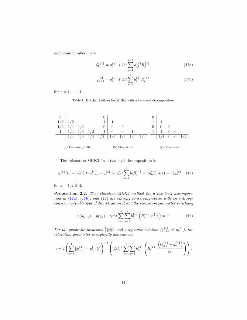
each zone number z are

Qzn,i = qzn +4t

i−1∑j=1

azij R

zj , (17a)

qzn+1 = qzn +4t

4∑i=1

bzi R

zi (17b)

for z = 1, · · · , 4.

Table 1: Butcher tableau for MRK2 with a two-level decomposition.

01/2 1/21/2 1/4 1/41 1/4 1/4 1/2

1/4 1/4 1/4 1/4

(a) Fast zone/buffer

01 10 0 01 0 0 1

1/4 1/4 1/4 1/4

(b) Slow buffer

01 10 0 01 1 0 0

1/2 0 0 1/2

(c) Slow zone

The relaxation MRK2 for a two-level decomposition is

qz(tn + γ4t) ≈ qzn+γ = qzn + γ4t4∑i=1

biRzi = γq

zn+1 + (1− γ)qzn (18)

for z = 1, 2, 3, 4.

Proposition 2.2. The relaxation MRK2 method for a two-level decomposi-tion in (17a), (17b), and (18) are entropy conserving/stable with an entropy-conserving/stable spatial discretization R and the relaxation parameter satisfying

η(qn+γ)− η(qn)− γ4t4∑z=1

s∑i=1

bzi

(Rzi , ϕ

zn,i

)= 0. (19)

For the quadratic invariant 12‖q‖

2 and a dynamic solution (qzn+1 6= q

zn ), the

relaxation parameter is explicitly determined:

γ = 2

(4∑z=1

‖qzn+1 − qzn ‖2)−1

(4t)24∑z=1

s∑i=1

bzi

Rzi ,

(Qzn,i − q

zn

)4t

.

11

Proof. The change in the entropy from tn to tn+γ becomes

η(qn+γ)− η(qn) = η(qn+γ)− η(qn)− γ4t4∑z=1

s∑i=1

bzi

(Rzi , ϕ

zn,i

)︸ ︷︷ ︸

:=θ(γ)

+ γ4t4∑z=1

s∑i=1

bzi

(Rzi , ϕ

zn,i

). (20)

By solving (19) for γ, the first, second, and third terms in (20) vanish justas in the IMEX case. With an entropy-conserving/stable spatial discretizationof R, the last term in (20) becomes again nonpositive.

By substituting η with the inner-product norm 12‖q‖

2 and by using (17b),(19) becomes

‖qn+γ‖2 − ‖qn‖2 − 2γ4t4∑z=1

s∑i=1

bzi

(Rzi , Q

zn,i

)= γ2‖qn+1−qn‖2 +2γ

4∑z=1

(qzn+1 − qzn , qzn

)−2γ4t

4∑z=1

s∑i=1

bzi

(Rzi , Q

zn,i

)= γ2‖qn+1 − qn‖2 − 2γ4t

4∑z=1

s∑i=1

bzi

(Rzi , Q

zn,i − q

zn

)= 0.

Rearranging the last equation yields an explicit form for γ.

At each stage, communication occurs between the fast zone and the fastbuffer and between the fast buffer and the slow buffer. However, communicationhappens only at two stages (1 and 4) between the slow buffer and the slow zone.6 Based on this observation, we group the fast zone, the fast buffer, and theslow buffer by a level block that has four stages, which we call a cycle. We willuse the level block notation for multilevel decomposition in the next section.

2.3.2. Beyond Two-Level Decomposition

We start by defining a level block. A level block (B) is formed by consecutiveelements with the same multirate level (`), each of which is assigned to a zonenumber (z). That means a level block (B) consists of a fast zone (fz), fast buffer(fb), and slow buffer (sb). 7 A level block (B) can have a neighbor level block(N(B)) that has `± 1 multirate level. We let Lmax be the maximum level and 0

6After exchanging the interface data at the fourth stage, the right-hand side of the slowbuffer at the second stage is evaluated.

7We view the fast zone of level ` as the slow zone with respect to level `+ 1. For instance,the level blocks with level 0 and level 1 in Figure 2 correspond to the fast zone, the bufferzone, and the slow zone in Figure 1.

12

be the minimum (root) level. We let sG := 2Lmax+1 be the total number of globalstages and let s0 = 2 and s`(B) = 4 (for ` = 1, 2, · · · ) be the total number oflocal stages of a level block (B). We also let m(B) := m`(B) = 2`(B)−1 be

the number of substeps and 4t`(B) :=(

12

)`(B)−14t be the local time step size

of a level block (B) so that m`(B)4t`(B) = 4t if `(B) > 0. When `(B) = 0,we take m(B) = 1. We assume that each fast buffer (fz) and slow buffer (sb)consist of one element.

The intermediate states and the next step solution of a level block (B) anda zone number (z) are written as

QB,zn+ k

m(B),i

= qB,zn+ k

m(B)

+4t`(B)i−1∑j=1

azij R

B,zn+ k

m(B),j, (21a)

qB,zn+1 = qB,zn +4t`(B)

m(B)∑r=1

s`(B)∑i=1

bzi R

B,zn+ r−1

m(B),i, (21b)

where

qB,zn+ k

m(B)

= qB,zn +4t`(B)k∑r=1

s`(B)∑i=1

bzi R

B,zn+ r−1

m(B),i,

for k = 0, 1, · · · ,m(B)− 1 and i = 1, · · · , s`(B).At the first global stage, all level blocks are activated, which means that the

intermediate states of all the level blocks are updated and exchanged betweenadjacent active level blocks. At the second and the third global stages, the levelblocks that have the maximum level Lmax are activated. At the fourth globalstage, the level blocks that have Lmax and Lmax−1 levels are activated. Thisimplies that after one cycle, these level blocks are synchronized. This process isrepeated until all the level blocks are synchronized at the last global stage, sG.We construct the activation table in Algorithm 2 to control the synchronization.That is, according to the activation table, certain level blocks are activated ata given global stage.

We give an example with a three-level decomposition in Figure 2, where threelevel blocks (B1, B2, and B3) have 0, 1, and 2 multirate levels, respectively. Themaximum level is two, Lmax = 2; thus the total number of global stage becomessG = 8. B1 and B2 have one subcycle (m(B1) = m(B2) = 1), and B3 hastwo subcycles (m(B3) = 2). At every subcycle, a level block (B) needs to besynchronized with its neighbors (N (B)). The B3 level block communicates withthe B2 level block at four stages (i.e., 1, 4, 5, and 8 global stages), whereas theB2 level block exchanges the interface data with the B1 level block at two stages(i.e., 1 and 8 global stages).

The intermediate states and the next step solution corresponding to Figure

13

Algorithm 2 Activation Table for Level Blocks

Ensure: Given the maximum level (Lmax), construct the activation table(actvTable) of the size sG × NB . Here, NB is the total number of levelblocks.

1: actvTable[:, :] = 02: for B in 1 : NB do3: nActv ← 2`(B)

4: d← 2(Lmax+1−`(B))

5: for i = 1 : nActv do6: actvTable[ 1 + d(i− 1), B]← 17: actvTable[sG − d(i− 1), B]← 18: end for9: end for

Three level problems• Each level is consists of Fast zone/ Fast Buffer/ Slow Buffer• Level2 slow buf talks with level1 fast zone at 1st, 4th, 5th, 8th stages• Level1 slow buf talks with level0 fast zone at 1st, 8th stages • Synchronization at 4th and 8th stages

Fast zone Fast ZoneFast Buf Slow Buf

4

1

Synchronization after 4th global stage

Fast Buf Slow Buf Fast Zone

8

5

Synchronization after 8th global stage

1

8

Level 2 Level 1 Level 0

Figure 2: Illustration of MRK2 with a three-level decomposition: three level blocks (B1, B2,and B3) have 0, 1, and 2 multirate levels, respectively. Each level block is composed of thefast zone, the fast buffer, and the slow buffer. The maximum level is two, Lmax = 2. Thenumber of global stages (the depth of MRK2) is 8(= 2Lmax+1), and the number of local stageof each level is 4 (except level 0). The B3 level block communicates with B2 level block atfour stages (i.e., 1, 4, 5, and 8 global stages), whereas the B2 level block exchanges interfacedata with the B1 level block at two stages (i.e., 1 and 8 global stages).

2 yield

QB1,zn,i = qB1,z

n + 24t2∑j=1

azij R

B1,zn,j i = 1, 2,

QB2,zn+ 0

1 ,i= qB2,z

n +4t4∑j=1

azij R

B2,zn,j i = 1, · · · , 4,

QB3,zn+ 0

2 ,i= qB3,z

n +4t2

4∑j=1

azij R

B3,zn,j i = 1, · · · , 4,

QB3,zn+ 1

2 ,i= qB3,zn+ 1

2

+4t2

4∑j=1

azij R

B3,zn+ 1

2 ,ji = 1, · · · , 4,

14

and

qB1,zn+1 = qB1,z

n + 24t2∑i=1

bzi R

B1,zn,i ,

qB2,zn+1 = qB2,z

n +4t4∑i=1

bzi R

B2,zn,i ,

qB3,zn+1 = qB3,z

n +4t2

2∑r=1

4∑i=1

bzi R

B3,zn+ r−1

2 ,i,

where

qB3,zn+ 1

2

= qB3,zn +

4t2

4∑i=1

bzi R

B3,zn,i ,

for z = 1, 2, 3.The relaxation MRK2 for multilevel decomposition is

qB,zn+γ = qB,zn + γ4t`(B)

m(B)∑r=1

s`(B)∑i=1

bzi R

B,zn+ r−1

m(B),i

(22)

for a level block B and a zone number z.

Proposition 2.3. Let NB be the number of level blocks. The relaxation MRK2method for multilevel decomposition in (21a), (21b), and (22) are entropy con-serving/stable with an entropy-conserving/stable spatial discretization R(q) andthe relaxation parameter

η(qn+γ)− η(qn)

− γNB∑B=1

4t`(B)3∑z=1

m(B)∑r=1

s`(B)∑i=1

bzi

(RB,zn+ r−1

m(B),i, ϕB,zn+ r−1

m(B),i

)= 0. (23)

For the quadratic invariant 12‖q‖

2, the relaxation parameter is explicitly deter-mined:

γ = 2

(NB∑B=1

3∑z=1

‖qB,zn+1 − qB,zn ‖2)−1

NB∑B=1

4t`(B)3∑z=1

m(B)∑r=1

s`(B)∑i=1

bzi

(RB,zn+ r−1

m(B),i, QB,zn+ r−1

m(B),i− qB,zn

) .

15

Proof. The change in the entropy from tn to tn+γ becomes

η(qn+γ)− η(qn) =

η(qn+γ)− η(qn)− γNB∑B=1

4t`(B)3∑z=1

m(B)∑r=1

s`(B)∑i=1

bzi

(RB,zn+ r−1

m(B),i, ϕB,zn+ r−1

m(B),i

)︸ ︷︷ ︸

:=θ(γ)

+ γ

NB∑B=1

4t`(B)3∑z=1

m(B)∑r=1

s`(B)∑i=1

bzi

(RB,zn+ r−1

m(B),i, ϕB,zn+ r−1

m(B),i

). (24)

By solving (23) for γ, the first, second, and third terms in (24) vanish asbefore. With an entropy-conserving/stable spatial discretization of R, the lastterm in (24) becomes nonpositive as expected.

By substituting η with the inner-product norm 12‖q‖

2 and using (21b), (23)becomes

‖qn+γ‖2−‖qn‖2−2γ

NB∑B=1

4t`(B)3∑z=1

m(B)∑r=1

s`(B)∑i=1

bzi

(RB,zn+ r−1

m(B),i, QB,zn+ r−1

m(B),i

)

= γ2‖qn+1 − qn‖2 + 2γ

NB∑B=1

3∑z=1

(qB,zn+1 − qB,zn , qB,zn

)

− 2γ

NB∑B=1

4t`(B)3∑z=1

m(B)∑r=1

s`(B)∑i=1

bzi

(RB,zn+ r−1

m(B),i, QB,zn+ r−1

m(B),i

)= γ2‖qn+1 − qn‖2

− 2γ

NB∑B=1

4t`(B)3∑z=1

m(B)∑r=1

s`(B)∑i=1

bzi

(RB,zn+ r−1

m(B),i, QB,zn+ r−1

m(B),i− qB,zn

)= 0.

Rearranging the last equation yields the explicit γ.

For implementation, first we balance the multirate level of each element sothat all the level blocks have a 2:1 local time step size ratio to their adjacentlevel blocks according to Algorithm 3. Next we construct the activation ta-ble in Algorithm 2. Then we compute the entropy-conserving/stable solutionsaccording to Algorithm 4.

3. Numerical Results

In this section we present several numerical experiments to demonstrate theentropy-conserving/stable properties of the proposed IMEX methods and themultirate methods. We compare standard methods, relaxation approaches, andincremental direction techniques for both IMEX and multirate methods. We usethe IMEX methods for handling scale-separable stiffness on uniform mesh and

16

Algorithm 3 Balancing Multirate Level of Elements

Ensure: Let K be the total number of elements. Let LE ∈ R be the initialmultirate levels of all elements. Let BLE ∈ R be the 2:1 balanced multiratelevels of all elements. That is, a level jump between adjacent elements isat most one. Given LE, BLE is created. Let bs be the buffer size of two.We assume that bs + 1 left/right boundary elements have the same level,LE(1:bs+1) = `left and LE((K−bs):K) = `right.

1: Compute level difference, δLE(1:K−1) = LE(2:K) − LE(1:K−1)

2: idx← Find(δLE 6= 0)3: cond = false; BLE ← LE4: while !cond do5: cond = true6: for i in 1 : length(idx) do7: iK1 ← idx[i]8: iK2 ← idx[i+ 1]9: if (δLE(iK1) == −1) and (δLE(iK2) == −1) then

10: if (iK2 − iK1) < (bs+ 1) then11: cond = false12: nc = (bs+ 1)− (iK2 − iK1)13: BLE(iK2+1:iK2+nc) = max(BLE(iK2+1:iK2+nc), LE(iK2))14: end if15: else if (δLE(iK1) == −1) and (δLE(iK2) == 1) then16: if (iK2 − iK1) < (bs+ 1) then17: cond = false18: BLE(iK1+1:iK2) = max(BLE(iK2), LE(iK1))19: end if20: else if (δLE(iK1) == 1) and (δLE(iK2) == 1) then21: cond = false22: if (iK2 − iK1) < (bs+ 1) then23: cond = false24: nc = (bs+ 1)− (iK2 − iK1)25: BLE(iK1+1−nc:iK1) = max(BLE(iK1+1−nc:iK1), LE(iK2))26: end if27: end if28: end for29: Update level of elements, LE ← BLE30: Compute level difference, δLE(1:K−1) := LE(2:K) − LE(1:K−1) ∈ RK−1

31: idx← Find(δLE 6= 0)32: end while

the multirate method for dealing with geometric-induced stiffness on nonuniform

17

meshes. We measure the L2 error of u by

‖qh − qr‖Ωh:=

( ∑K∈Ωh

(qh − qr, qh − qr)K

) 12

,

where qr is either an exact solution or a reference solution and (·, ·)K is theL2 inner product on an element K ∈ Ωh. The total entropy loss and the totalmass loss are defined by |η(t)− η(0)| and |mass(t)−mass(t)|, where mass(t) :=(qh,1)Ωh

.

3.1. ODEs: Conserved Exponential Entropy

We consider the ODE example [39] preserving exponential entropy

η(q) = exp(q1) + exp(q2).

The ODE system is given by

d

dt

(q1

q2

)=

(− exp(q2)exp(q1)

),

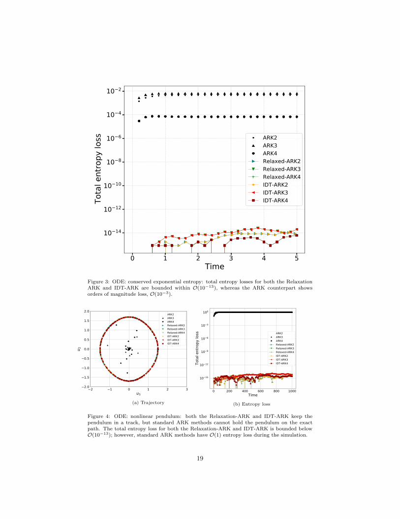
with the initial condition of q = (1, 0.5)T . We take 4t = 0.1 and run thesimulations for t ∈ [0, 5]. We plot the time series of the exponential entropy inFigure 3. We observe that the total entropy loss for both the Relaxation-ARKand IDT-ARK are below O(10−13), whereas the standard ARK counterpartshows orders of magnitude loss, such as O(10−3), as expected.

3.2. ODE: Nonlinear Pendulum

The nonlinear pendulum [39] ODE system is given by

d

dt

(q1

q2

)=

(− sin(q2)

q1

),

with the initial condition q = (1.5, 0)T and the entropy function η(q) = 0.5q21 −

cos(q2). We examine the entropy behavior and the solution trajectory over timein Figure 4. We take 4t = 0.9 and run the simulations for t ∈ [0, 1000]. Boththe Relaxation-ARK and IDT-ARK keep the pendulum in a track, but standardARK methods cannot hold the pendulum in the path. The total entropy lossfor both the Relaxation-ARK and IDT-ARK are bounded within O(10−13);however, as expected, standard ARK methods have O(1) entropy loss duringthe simulation.

3.3. Entropy-Stable IMEX for the Burgers Equation on Uniform Mesh

We consider a Gaussian initial profile, which develops a shock as time passesfor the Burgers equation. The initial condition is given as

q = exp(−10x2)

18

0 1 2 3 4 5Time

10 14

10 12

10 10

10 8

10 6

10 4

10 2

Tota

l ent

ropy

loss ARK2

ARK3ARK4Relaxed-ARK2Relaxed-ARK3Relaxed-ARK4IDT-ARK2IDT-ARK3IDT-ARK4

Figure 3: ODE: conserved exponential entropy: total entropy losses for both the RelaxationARK and IDT-ARK are bounded within O(10−13), whereas the ARK counterpart showsorders of magnitude loss, O(10−3).

2 1 0 1 2 3u1

2.0

1.5

1.0

0.5

0.0

0.5

1.0

1.5

2.0

u 2

ARK2ARK3ARK4Relaxed-ARK2Relaxed-ARK3Relaxed-ARK4IDT-ARK2IDT-ARK3IDT-ARK4

(a) Trajectory

0 200 400 600 800 1000Time

10 15

10 12

10 9

10 6

10 3

100

Tota

l ent

ropy

loss ARK2

ARK3ARK4Relaxed-ARK2Relaxed-ARK3Relaxed-ARK4IDT-ARK2IDT-ARK3IDT-ARK4

(b) Entropy loss

Figure 4: ODE: nonlinear pendulum: both the Relaxation-ARK and IDT-ARK keep thependulum in a track, but standard ARK methods cannot hold the pendulum on the exactpath. The total entropy loss for both the Relaxation-ARK and IDT-ARK is bounded belowO(10−13); however, standard ARK methods have O(1) entropy loss during the simulation.

19

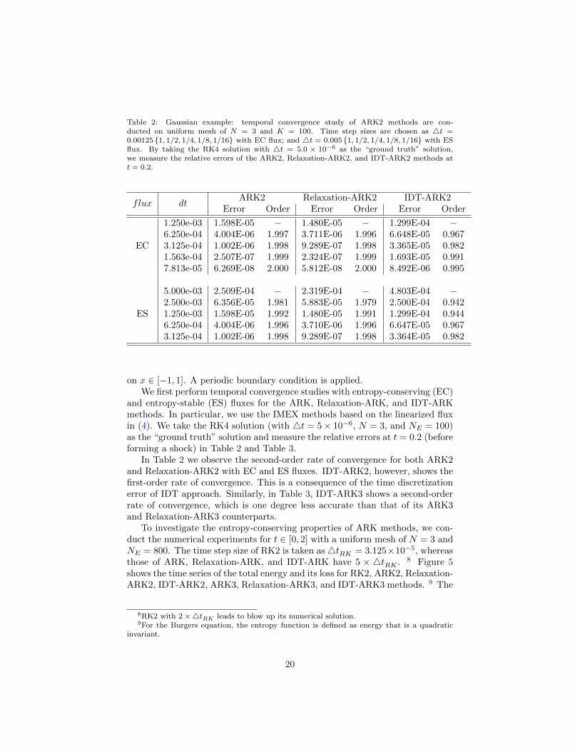
Table 2: Gaussian example: temporal convergence study of ARK2 methods are con-ducted on uniform mesh of N = 3 and K = 100. Time step sizes are chosen as 4t =0.00125 1, 1/2, 1/4, 1/8, 1/16 with EC flux; and 4t = 0.005 1, 1/2, 1/4, 1/8, 1/16 with ESflux. By taking the RK4 solution with 4t = 5.0 × 10−6 as the “ground truth” solution,we measure the relative errors of the ARK2, Relaxation-ARK2, and IDT-ARK2 methods att = 0.2.

flux dtARK2 Relaxation-ARK2 IDT-ARK2

Error Order Error Order Error Order

1.250e-03 1.598E-05 − 1.480E-05 − 1.299E-04 −6.250e-04 4.004E-06 1.997 3.711E-06 1.996 6.648E-05 0.967

EC 3.125e-04 1.002E-06 1.998 9.289E-07 1.998 3.365E-05 0.9821.563e-04 2.507E-07 1.999 2.324E-07 1.999 1.693E-05 0.9917.813e-05 6.269E-08 2.000 5.812E-08 2.000 8.492E-06 0.995

5.000e-03 2.509E-04 − 2.319E-04 − 4.803E-04 −2.500e-03 6.356E-05 1.981 5.883E-05 1.979 2.500E-04 0.942

ES 1.250e-03 1.598E-05 1.992 1.480E-05 1.991 1.299E-04 0.9446.250e-04 4.004E-06 1.996 3.710E-06 1.996 6.647E-05 0.9673.125e-04 1.002E-06 1.998 9.289E-07 1.998 3.364E-05 0.982

on x ∈ [−1, 1]. A periodic boundary condition is applied.We first perform temporal convergence studies with entropy-conserving (EC)

and entropy-stable (ES) fluxes for the ARK, Relaxation-ARK, and IDT-ARKmethods. In particular, we use the IMEX methods based on the linearized fluxin (4). We take the RK4 solution (with 4t = 5× 10−6, N = 3, and NE = 100)as the “ground truth” solution and measure the relative errors at t = 0.2 (beforeforming a shock) in Table 2 and Table 3.

In Table 2 we observe the second-order rate of convergence for both ARK2and Relaxation-ARK2 with EC and ES fluxes. IDT-ARK2, however, shows thefirst-order rate of convergence. This is a consequence of the time discretizationerror of IDT approach. Similarly, in Table 3, IDT-ARK3 shows a second-orderrate of convergence, which is one degree less accurate than that of its ARK3and Relaxation-ARK3 counterparts.

To investigate the entropy-conserving properties of ARK methods, we con-duct the numerical experiments for t ∈ [0, 2] with a uniform mesh of N = 3 andNE = 800. The time step size of RK2 is taken as 4tRK = 3.125×10−5, whereasthose of ARK, Relaxation-ARK, and IDT-ARK have 5 × 4tRK . 8 Figure 5shows the time series of the total energy and its loss for RK2, ARK2, Relaxation-ARK2, IDT-ARK2, ARK3, Relaxation-ARK3, and IDT-ARK3 methods. 9 The

8RK2 with 2×4tRK leads to blow up its numerical solution.9For the Burgers equation, the entropy function is defined as energy that is a quadratic

invariant.

20

Table 3: Same as 2, except the third-order accurate methods.

flux dtARK3 Relaxation-ARK3 IDT-ARK3

Error Order Error Order Error Order

1.250e-03 4.755E-07 − 4.533E-07 − 1.018E-05 −6.250e-04 6.027E-08 2.980 5.762E-08 2.976 2.539E-06 2.003

EC 3.125e-04 7.612E-09 2.985 7.290E-09 2.983 6.340E-07 2.0021.563e-04 9.578E-10 2.990 9.184E-10 2.989 1.584E-07 2.0017.813e-05 1.202E-10 2.994 1.154E-10 2.992 3.959E-08 2.000

5.000e-03 2.757E-05 − 2.575E-05 − 1.647E-04 −2.500e-03 3.609E-06 2.933 3.410E-06 2.917 4.088E-05 2.010

ES 1.250e-03 4.594E-07 2.974 4.364E-07 2.966 1.018E-05 2.0066.250e-04 5.787E-08 2.989 5.511E-08 2.985 2.539E-06 2.0033.125e-04 7.260E-09 2.995 6.922E-09 2.993 6.340E-07 2.002

0.00

0.25

0.50

0.75

1.00

1.25

1.50

1.75

2.00

Time

3.4 × 100

3.6 × 100

3.8 × 100

4 × 100

4.2 × 100

4.4 × 100

Tota

l ene

rgy

RK2ARK2ARK2 (Relaxation)ARK2 (IDT)ARK3ARK3 (Relaxation)ARK3 (IDT)

(a) Total Energy History (EC)

0.25

0.50

0.75

1.00

1.25

1.50

1.75

2.00

Time

10 16

10 14

10 12

10 10

10 8

10 6

10 4

10 2

100

Tota

l ene

rgy

loss RK2

ARK2ARK2 (Relaxation)ARK2 (IDT)ARK3ARK3 (Relxation)ARK3 (IDT)

(b) Total Energy Loss (EC)

Figure 5: Histories of total entropy and its loss of Gaussian example for the Burgers equationwith EC flux: the relaxation methods with EC flux conserve the total energy within O(10−13).

second- and the third-order Relaxation-ARK and IDT-ARK methods conservetheir total energies within O(10−13) losses, whereas ARK2 and ARK3 show aslightly decreasing trend of total energy. This is because IMEX methods act asa high-frequency filter by treating the fast-varying dynamics implicitly [7, 46].As a result, energy-stable behavior is observed for the standard ARK methods.RK2, however, does not have any filter functionality, so its total energy showsan increasing trend.

We show snapshots at t = 1 in Figure 6. All numerical solutions sufferfrom high-frequency noise arising from the Gibbs phenomenon in the presenceof a shock. However, the numerical solutions do not blow up thanks to theskew-symmetric formulation [23]. Compared with RK2, ARK2 dramaticallyeliminates the high-frequency oscillation. Relaxation-ARK2 and IDT-ARK2also reduce the high-frequency oscillation but not as significantly as ARK2.

21

1.00

0.75

0.50

0.25

0.00

0.25

0.50

0.75

1.00

x

0.5

1.0

1.5

2.0

2.5

3.0

u

time= 1.000

(a) RK2

1.00

0.75

0.50

0.25

0.00

0.25

0.50

0.75

1.00

x

0.5

1.0

1.5

2.0

2.5

3.0

u

time= 1.000

(b) ARK2

1.00

0.75

0.50

0.25

0.00

0.25

0.50

0.75

1.00

x

0.5

1.0

1.5

2.0

2.5

3.0

u

time= 1.000

(c) Relaxation-ARK2

1.00

0.75

0.50

0.25

0.00

0.25

0.50

0.75

1.00

x

0.5

1.0

1.5

2.0

2.5

3.0

u

time= 1.000

(d) IDT-ARK2

Figure 6: Snapshots of Gaussian profile for Burgers equation at t = 1: (a) RK2, (b) ARK2,(c) Relaxation-ARK2, and (d) IDT-ARK2. The time step size of RK2 is taken as 4tRK =3.125 × 10−5, whereas those of ARK2, Relaxation-ARK2, and IDT-ARK2 have 5 × 4tRK .The domain is discretized with a uniform mesh of N = 3 and NE = 800.

22

Next, we examine the entropy-stable properties of ARK methods. The Lax–Friedrichs (LF) flux with the skew-symmetric formulation yields the energy-stable DG method [23]. We perform the simulations for t ∈ [0, 2] with N = 3 andNE = 800. The time step size of RK2 is taken as 4tRK = 2.5× 10−4, whereasthose of the other methods including the ARK2 method have 2.5 ×4tRK . 10

Compared with EC flux, LF flux substantially eliminates numerical oscillations,but still not enough to remove nonphysical oscillations near shocks. Thus, weadditionally apply the limiter in (5a) to a marched solution at every time step.

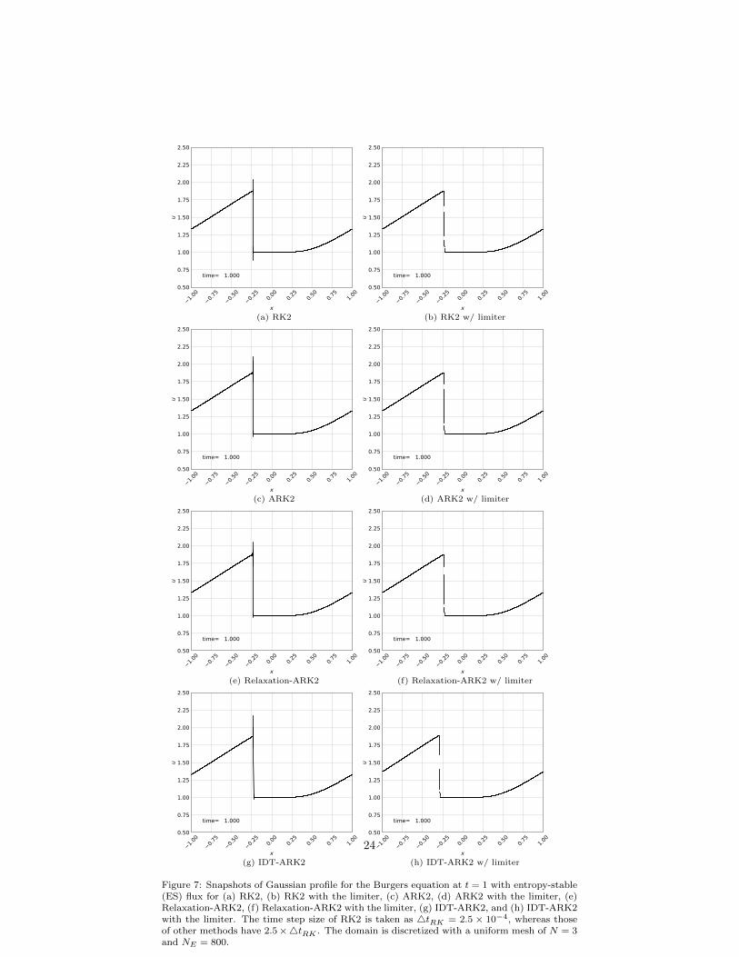
The snapshots at t = 1 are reported in Figure 7. All the methods withthe limiter successfully eliminate the spurious oscillations near the shock front.The shock front, located near x = −0.25, is well captured for all methodswith/without the limiter. However, IDT-ARK2 methods (with/without thelimiter) show the shock position error compared with other methods.

In Figure 8, the time histories of the total energy and its loss are reportedfor ARK2, Relaxation-ARK2, IDT-ARK2, ARK3, Relaxation-ARK3, and IDT-ARK3 with/without the limiter. (The RK2 result is also reported for compar-ison.) All the methods with ES flux show entropy-stable behaviors regardlessof applying the limiter. This observation agrees with the work in [28, Theorem3.8].

In Figure 9 we also plot the time series of the total mass (a linear invariant)for ARK2, Relaxation-ARK2, IDT-ARK2, ARK3, Relaxation-ARK3, and IDT-ARK3 with/ without limiter, as well as RK2. As expected, all the methodspreserve the total mass within O(10−14).

3.4. Entropy–stable Multirate methods for Burgers equation on non–uniformmesh

We consider MRK2 methods on a nonuniform mesh for handling geometric-induced stiffness. 11 A one-dimensional domain is five times refined at thecenter of the domain with a 2:1 grid ratio so that the biggest element is 32times larger than the smallest element, as shown in Figure 10a. In the MRK2algorithm, based on the ratio of the element sizes, multirate levels are assignedto each element in Figure 10b, where the highest multirate level is five.

We first perform temporal convergence studies with the entropy-conservingand entropy-stable fluxes for MRK2, Relaxation-MRK2, and IDT-MRK2 meth-ods. We take the RK4 solution (with 4t = 5× 10−6, N = 3, and NE = 196) asthe “ground truth” solution and measure the relative errors at t = 0.2 (beforeforming a shock) in Table 4.

The numerical solutions converge to the reference RK4 solution with second-order accuracy for the MRK2, Relaxation-MRK2, and IDT-MRK2 methodsregardless of the EC/ES fluxes. The errors of Relaxation-MRK2 and IDT-MRK2 are even the same in Table 4. This is because their relaxation parameters

10RK2 with 4tRK = 5× 10−4 leads to blowup the numerical solution.11IMEX methods can also be utilized for dealing with geometric-induced stiffness but require

a linear/nonlinear solve at each stage in general. Thus, we focus on the MRK2 method, whichdoes not require any linear/nonlinear solves.

23

1.00

0.75

0.50

0.25

0.00

0.25

0.50

0.75

1.00

x

0.50

0.75

1.00

1.25

1.50

1.75

2.00

2.25

2.50

u

time= 1.000

(a) RK2

1.00

0.75

0.50

0.25

0.00

0.25

0.50

0.75

1.00

x

0.50

0.75

1.00

1.25

1.50

1.75

2.00

2.25

2.50

u

time= 1.000

(b) RK2 w/ limiter

1.00

0.75

0.50

0.25

0.00

0.25

0.50

0.75

1.00

x

0.50

0.75

1.00

1.25

1.50

1.75

2.00

2.25

2.50

u

time= 1.000

(c) ARK2

1.00

0.75

0.50

0.25

0.00

0.25

0.50

0.75

1.00

x

0.50

0.75

1.00

1.25

1.50

1.75

2.00

2.25

2.50

u

time= 1.000

(d) ARK2 w/ limiter

1.00

0.75

0.50

0.25

0.00

0.25

0.50

0.75

1.00

x

0.50

0.75

1.00

1.25

1.50

1.75

2.00

2.25

2.50

u

time= 1.000

(e) Relaxation-ARK2

1.00

0.75

0.50

0.25

0.00

0.25

0.50

0.75

1.00

x

0.50

0.75

1.00

1.25

1.50

1.75

2.00

2.25

2.50

u

time= 1.000

(f) Relaxation-ARK2 w/ limiter

1.00

0.75

0.50

0.25

0.00

0.25

0.50

0.75

1.00

x

0.50

0.75

1.00

1.25

1.50

1.75

2.00

2.25

2.50

u

time= 1.000

(g) IDT-ARK2

1.00

0.75

0.50

0.25

0.00

0.25

0.50

0.75

1.00

x

0.50

0.75

1.00

1.25

1.50

1.75

2.00

2.25

2.50

u

time= 1.000

(h) IDT-ARK2 w/ limiter

Figure 7: Snapshots of Gaussian profile for the Burgers equation at t = 1 with entropy-stable(ES) flux for (a) RK2, (b) RK2 with the limiter, (c) ARK2, (d) ARK2 with the limiter, (e)Relaxation-ARK2, (f) Relaxation-ARK2 with the limiter, (g) IDT-ARK2, and (h) IDT-ARK2with the limiter. The time step size of RK2 is taken as 4tRK = 2.5 × 10−4, whereas thoseof other methods have 2.5×4tRK . The domain is discretized with a uniform mesh of N = 3and NE = 800.

24

0.00

0.25

0.50

0.75

1.00

1.25

1.50

1.75

2.00

Time

3.35 × 100

3.375 × 100

3.4 × 100

3.425 × 100

3.45 × 100

3.475 × 100

3.5 × 100

3.525 × 100

3.55 × 100To

tal e

nerg

yRK2ARK2ARK2 (Relaxation)ARK2 (IDT)ARK3ARK3 (Relaxation)ARK3 (IDT)ARK2 (limiter)ARK2 (limiter,Relaxation)ARK2 (limiter,IDT)ARK3 (limiter)ARK3 (limiter,Relaxation)ARK3 (limiter,IDT)

(a) Total Energy History (ES)

0.25

0.50

0.75

1.00

1.25

1.50

1.75

2.00

Time

10 16

10 14

10 12

10 10

10 8

10 6

10 4

10 2

100

Tota

l ene

rgy

loss

RK2ARK2ARK2 (Relxation)ARK2 (IDT)ARK3ARK3 (Relxation)ARK3 (IDT)ARK2 (limiter)ARK2 (limiter,Relxation)ARK2 (limiter,IDT)ARK3 (limiter)ARK3 (limiter,Relxation)ARK3 (limiter,IDT)

(b) Total Energy Loss (ES)

Figure 8: Gaussian example for the Burger equation: histories of total energy and its losswith ES flux for ARK methods (standard, relaxation, and IDT). All the methods with ESflux show entropy-stable behaviors.

0.25

0.50

0.75

1.00

1.25

1.50

1.75

2.00

Time

10 16

10 14

10 12

10 10

10 8

10 6

10 4

10 2

100

Tota

l mas

s erro

r

RK2ARK2ARK2 (Relxation)ARK2 (IDT)ARK3ARK3 (Relxation)ARK3 (IDT)ARK2 (limiter)ARK2 (limiter,Relxation)ARK2 (limiter,IDT)ARK3 (limiter)ARK3 (limiter,Relxation)ARK3 (limiter,IDT)

Figure 9: Histories of total mass loss of Gaussian example for the Burgers equation with ESflux: without limiter, the methods preserve the total mass within O(10−14).

25

(a) h/hmin(b) MR levels for Lmax = 5

Figure 10: (a) Ratio of element sizes with respect to the minimum size of the elements and(b) multirate levels of elements for L = 5. Here, L is the maximum multirate (MR) level.The center of the domain is five times refined with a 2 : 1 ratio so that the largest elementis 32 times bigger than the smallest element. Multirate level is assigned to each elementcorresponding to the ratio of element sizes.

are small enough (O(10−5)) to conceal the difference between the relaxationand the IDT approaches. This agrees with the previous study in [33, Figure9.], where both IDT-RK2 and Relaxation-RK2 show the second-order rate ofconvergence in time. When the limiter is applied, however, the two approachesreveal a significant difference. We will discuss this issue later.

Next, we examine the entropy conservation of MRK2 methods. We performthe simulations for t ∈ [0, 2] with N = 3 and K = 784 (Lmax = 5). The time stepsize of RK2 is taken as4tRK = 6.25×10−6, whereas those of MRK2, Relaxation-MRK2, and IDT-MRK2 have 4t = 20 ×4tRK . 12 Figure 11 shows the timehistories of the total energy and its loss for RK2, Relax-RK2, IDT-RK2, MRK2,Relax-MRK2, and IDT-MRK2 methods. We see that both the relaxation andthe IDT methods preserve the total energy during the simulation. The loss ofthe total energy for the relaxation and the IDT methods is around O(10−13),whereas the standard RK2 and MRK2 counterparts increase to O(10−1). Wealso show the snapshots at t = 1 in Figure 12. As expected, high oscillatorynoises are observed, but numerical solutions are still stable.

Now, we examine the entropy stability of MRK2 methods with LF flux. Weperform the simulations for t ∈ [0, 2] with N = 3 and K = 784 (Lmax = 5). Thetime step size of RK2 is taken as 4tRK = 5 × 10−5, whereas those of MRK2,Relaxation-MRK2, and IDT-MRK2 have4t = 25×4tRK . 13 The snapshots att = 1 are reported in Figure 13. Similar to Figure 7, the IDT method suffers fromphase errors. The shock front of IDT-MRK2 is slightly lagged behind, and theerror becomes severe when limiter is applied. This example demonstrates that

12RK2 with 4tRK = 1.25× 10−6 leads to blowup of its numerical solution.13RK2 with 4tRK = 6.25× 10−5 yields a blowup solution.

26

0.00

0.25

0.50

0.75

1.00

1.25

1.50

1.75

2.00

Time

3.5 × 100

3.55 × 100

3.6 × 100

3.65 × 100

3.7 × 100

3.75 × 100

3.8 × 100

3.85 × 100

3.9 × 100

Tota

l ene

rgy

RK2RK2 (Relaxation)RK2 (IDT)MRK2MRK2 (Relaxation)MRK2 (IDT)

(a) Total Energy History (EC)

0.25

0.50

0.75

1.00

1.25

1.50

1.75

2.00

Time

10 16

10 14

10 12

10 10

10 8

10 6

10 4

10 2

100

Tota

l ene

rgy

loss

RK2RK2 (Relaxation)RK2 (IDT)MRK2MRK2 (Relaxation)MRK2 (IDT)

(b) Total Energy Loss (EC)

Figure 11: Histories of total energy and its loss of Gaussian example for the Burger equationwith EC flux: the relaxation methods with EC flux conserve the total energy within O(10−13).

1.00

0.75

0.50

0.25

0.00

0.25

0.50

0.75

1.00

x

0.5

1.0

1.5

2.0

2.5

3.0

u

time= 1.000

(a) RK2

1.00

0.75

0.50

0.25

0.00

0.25

0.50

0.75

1.00

x

0.5

1.0

1.5

2.0

2.5

3.0

u

time= 1.000

(b) MRK2

1.00

0.75

0.50

0.25

0.00

0.25

0.50

0.75

1.00

x

0.5

1.0

1.5

2.0

2.5

3.0

u

time= 1.000

(c) Relaxation MRK2

1.00

0.75

0.50

0.25

0.00

0.25

0.50

0.75

1.00

x

0.5

1.0

1.5

2.0

2.5

3.0

u

time= 1.000

(d) Relaxation MRK2 (IDT)

Figure 12: Snapshots of Gaussian profile for the Burgers equation at t = 1 on a nonuniformmesh with energy-conserving (EC) flux for (a) RK2, (b) MRK2, (c) Relaxation-MRK2, and(d) IDT-MRK2. The time step size of RK2 is taken as 4tRK = 6.25×10−6, whereas those ofMRK2, Relaxation-MRK2, and IDT-MRK2 have 4t = 20×4tRK . The domain is discretizedwith a nonuniform mesh of N = 3 and K = 784 (Lmax = 5).

27

Table 4: Gaussian example: temporal convergence study for MRK2 methods performed withEC and ES fluxes on nonuniform mesh of N = 3 and K = 196. We use the time step sizeswith 4t = 0.001 1, 1/2, 1/4, 1/8, 1/16 for EC flux and 4t = 0.0025 1, 1/2, 1/4, 1/8, 1/16for ES flux. By taking the RK4 solution with 4t = 5.0×10−6 as “ground truth” solution, wemeasure the relative errors of MRK2, Relaxation-MRK2, and IDT-MRK2 methods at t = 0.2.

flux dtMRK2 Relaxation-MRK2 IDT-MRK2

Error Order Error Order Error Order

1.000e-03 5.673E-06 − 5.597E-06 − 5.597E-06 −5.000e-04 1.434E-06 1.984 1.415E-06 1.983 1.415E-06 1.983

EC 2.500e-04 3.609E-07 1.990 3.564E-07 1.990 3.564E-07 1.9901.250e-04 9.054E-08 1.995 8.941E-08 1.995 8.941E-08 1.9956.250e-05 2.267E-08 1.998 2.239E-08 1.998 2.239E-08 1.998

2.500e-03 7.425E-05 − 9.407E-05 − 9.407E-05 −1.250e-03 1.683E-05 2.141 1.788E-05 2.395 1.788E-05 2.395

ES 6.250e-04 4.020E-06 2.066 4.043E-06 2.145 4.043E-06 2.1453.125e-04 9.829E-07 2.032 9.770E-07 2.049 9.770E-07 2.0491.563e-04 2.431E-07 2.015 2.413E-07 2.018 2.413E-07 2.018

the relaxation approach is better than the IDT approach in terms of accuracy,especially when a limiter is applied.

Figure 14 shows the time histories of the total entropy and its loss for theRK2, Relaxation-RK2, IDT-RK2, MRK2, Relaxation-MRK2, and IDT-MRK2methods with/without limiter. All the methods show entropy-stable behaviors.The entropy losses of all methods reach O(10−1) as time passes. In Figure 15 thetime history of the total mass loss is shown for the RK2, Relaxation-RK2, IDT-RK2, MRK2, Relaxation-MRK2, and IDT-MRK2 methods with/without thelimiter. In general, all the methods demonstrate good total mass conservation.In particular, without the limiter, all the methods preserve the total mass withinO(10−14) error. With the limiter, however, the total mass loss is boundedby O(10−12) for the RK2, Relaxation-RK2, and IDT-RK2 methods and byO(10−13) for the MRK2, Relaxation-MRK2, and IDT-MRK2 methods.

4. Conclusions

In this paper we present entropy-stable time discretization methods by us-ing a relaxation method for partitioned Runge–Kutta schemes. In particular weapply relaxation to IMEX–RK methods to solve stiff problems and to a class ofexplicit second-order multirate methods with grid-induced stiffness. The relax-ation methods successfully extend to both the IMEX–RK and multirate methodsfor targeting stiff problems in combination with an entropy-conserving/stablespatial discretization. We demonstrate the entropy conservation and stabilityproperties for a few ODEs and the Burgers equation when using relaxation

28

1.00

0.75

0.50

0.25

0.00

0.25

0.50

0.75

1.00

x

0.50

0.75

1.00

1.25

1.50

1.75

2.00

2.25

2.50

u

time= 1.000

(a) RK2

1.00

0.75

0.50

0.25

0.00

0.25

0.50

0.75

1.00

x

0.50

0.75

1.00

1.25

1.50

1.75

2.00

2.25

2.50

u

time= 1.000

(b) RK2 w/ limiter

1.00

0.75

0.50

0.25

0.00

0.25

0.50

0.75

1.00

x

0.50

0.75

1.00

1.25

1.50

1.75

2.00

2.25

2.50

u

time= 1.000

(c) MRK2

1.00

0.75

0.50

0.25

0.00

0.25

0.50

0.75

1.00

x

0.50

0.75

1.00

1.25

1.50

1.75

2.00

2.25

2.50

u

time= 1.000

(d) MRK2 w/ limiter

1.00

0.75

0.50

0.25

0.00

0.25

0.50

0.75

1.00

x

0.50

0.75

1.00

1.25

1.50

1.75

2.00

2.25

2.50

u

time= 1.000

(e) Relaxation-MRK2

1.00

0.75

0.50

0.25

0.00

0.25

0.50

0.75

1.00

x

0.50

0.75

1.00

1.25

1.50

1.75

2.00

2.25

2.50

u

time= 0.998

(f) Relaxation-MRK2 w/ limiter

1.00

0.75

0.50

0.25

0.00

0.25

0.50

0.75

1.00

x

0.50

0.75

1.00

1.25

1.50

1.75

2.00

2.25

2.50

u

time= 1.000

(g) IDT-MRK2

1.00

0.75

0.50

0.25

0.00

0.25

0.50

0.75

1.00

x

0.50

0.75

1.00

1.25

1.50

1.75

2.00

2.25

2.50

u

time= 1.000

(h) IDT-MRK2 w/ limiter

Figure 13: Snapshots of Gaussian profile for the Burgers equation at t = 1 on a nonuniformmesh with entropy stable (ES) flux for (a) RK2, (b) RK2 with limiter, (c) MRK2, (d) MRK2with limiter, (e) Relaxation-MRK2, (f) Relaxation-MRK2 with limiter, (g) IDT-MRK2, and(h) IDT-MRK2 with limiter. The time step size of RK2 is taken as4tRK = 5×10−5, whereasthose of MRK2, Relaxation-MRK2, and IDT-MRK2 have 4t = 25 ×4tRK . The domain isdiscretized with a nonuniform mesh of N = 3 and K = 784 (Lmax = 5).

29

0.00

0.25

0.50

0.75

1.00

1.25

1.50

1.75

2.00

Time

3.35 × 100

3.375 × 100

3.4 × 100

3.425 × 100

3.45 × 100

3.475 × 100

3.5 × 100

3.525 × 100

3.55 × 100

Tota

l ene

rgy

RK2RK2 (Relaxation)RK2 (IDT)MRK2MRK2 (Relaxation)MRK2 (IDT)RK2 (limiter)RK2 (limiter,Relaxation)RK2 (limiter,IDT)MRK2 (limiter)MRK2 (limiter,Relaxation)MRK2 (limiter,IDT)

(a) Total Energy History (ES)

0.25

0.50

0.75

1.00

1.25

1.50

1.75

2.00

Time

10 16

10 14

10 12

10 10

10 8

10 6

10 4

10 2

100

Tota

l ene

rgy

loss

RK2RK2 (Relaxation)RK2 (IDT)MRK2MRK2 (Relaxation)MRK2 (IDT)RK2 (limiter)RK2 (limiter,Relaxation)RK2 (limiter,IDT)MRK2 (limiter)MRK2 (limiter,Relaxation)MRK2 (limiter,IDT)

(b) Total Energy Loss (ES)

Figure 14: Histories of total entropy and its loss of Gaussian example for the Burgers equationwith ES flux: all the methods with ES flux show entropy-stable behaviors.

0.25

0.50

0.75

1.00

1.25

1.50

1.75

2.00

Time

10 16

10 14

10 12

10 10

10 8

10 6

10 4

10 2

100

Tota

l mas

s erro

r

RK2RK2 (Relaxation)RK2 (IDT)MRK2MRK2 (Relaxation)MRK2 (IDT)RK2 (limiter)RK2 (limiter,Relaxation)RK2 (limiter,IDT)MRK2 (limiter)MRK2 (limiter,Relaxation)MRK2 (limiter,IDT)

Figure 15: Histories of total mass loss of Gaussian example for the Burgers equation with ESflux: without the limiter, the methods preserve the total mass within O(10−14). However,the limiting procedure somehow affects the mass loss quantity, but the methods are boundedby O(10−12)

30

IMEX-RK methods and the relaxation multirate method. In particular, wefocus on relaxation IMEX-RK methods on a uniform mesh to tackle scale-separable stiffness. This is achieved by defining the linearized flux containing thefast wave in the system with the stiffness being implicitly treated, thus allowingfor a longer time step size than that restricted by explicit methods. In addition,relaxation IMEX-RK methods not only support high-order accuracy in timebut also have entropy-conserving/stable properties if entropy-conserving/stablefluxes are equipped with them.

We have also studied the multirate method on a nonuniform mesh to han-dle geometric-induced stiffness arising from mesh refinements. Unlike IMEX-RK methods, multirate methods do not require any linear/nonlinear solve and,hence, are attractive for parallel computing if proper preconditioning is notavailable. Multirate methods decompose the original problem into subprob-lems, where different time step sizes can be used locally on each subproblem.We have numerically demonstrated that the Relaxation-MRK2 method has asecond-order rate of convergence and shows the total entropy-conserving/stablebehavior if entropy-conserving/stable spatial discretization is provided.

We observed that the relaxation approach is one degree more accurate thanthe incremental direction technique. Especially when shock occurs, the loca-tion error of the incremental direction technique becomes larger than with therelaxation approach. The error becomes severe when the limiter is applied.

Future work will focus on extension to multidimensions as well as otherpartial differential equations, including Euler equations, to exploit a nonlin-ear entropy. Developing entropy-conserving/stable coupling methods is also ofinterest.

Acknowledgments

This material is based upon work supported by the U.S. Department ofEnergy, Office of Science, Office of Advanced Scientific Computing Research(ASCR) and Office of Biological and Environmental Research (BER), ScientificDiscovery through Advanced Computing (SciDAC) program under ContractDE-AC02-06CH11357 through the Coupling Approaches for Next-GenerationArchitectures (CANGA) Project and ASCR Base Program.

Declaration

Availability of data and material

The datasets generated during and/or analyzed during the current study areavailable from the corresponding author on reasonable request.

Code availability

The code used to generate the results is not available.

31

[1] U. M. Ascher, S. J. Ruuth, R. J. Spiteri, Implicit-explicit Runge-Kuttamethods for time-dependent partial differential equations, Applied Numer-ical Mathematics 25 (2) (1997) 151–167.

[2] E. M. Constantinescu, A. Sandu, Multirate timestepping methods for hy-perbolic conservation laws, Journal of Scientific Computing 33 (3) (2007)239–278.

[3] F. X. Giraldo, M. Restelli, M. Lauter, Semi-implicit formulations of theNavier–Stokes equations: Application to nonhydrostatic atmospheric mod-eling, SIAM Journal on Scientific Computing 32 (6) (2010) 3394–3425.

[4] D. J. Gardner, J. E. Guerra, F. P. Hamon, D. R. Reynolds, P. A. Ullrich,C. S. Woodward, Implicit–explicit (IMEX) Runge–Kutta methods for non-hydrostatic atmospheric models, Geoscientific Model Development 11 (4)(2018) 1497–1515.

[5] C. Newman, G. Womeldorff, D. A. Knoll, L. Chacon, A communication-avoiding implicit–explicit method for a free-surface ocean model, Journalof Computational Physics 305 (2016) 877–894.

[6] J.-F. Lemieux, D. A. Knoll, M. Losch, C. Girard, A second-order accuratein time implicit–explicit (imex) integration scheme for sea ice dynamics,Journal of Computational Physics 263 (2014) 375–392.

[7] S. Kang, F. X. Giraldo, T. Bui-Thanh, IMEX HDG-DG: A coupled implicithybridized discontinuous Galerkin and explicit discontinuous Galerkin ap-proach for shallow water systems, Journal of Computational Physics (2019)109010.

[8] S. Streiner, S. Hauptmann, M. Kuhn, E. Kramer, Coupled fluid-structuresimulations of a wind turbine rotor, in: Deutsche Windenergie-Konferenz(DEWEK), Bremen, Germany, DEWI-German Wind Energy Institute,2008.

[9] S. T. Miller, E. C. Cyr, J. N. Shadid, R. M. J. Kramer, E. G. Phillips,S. Conde, R. P. Pawlowski, Imex and exact sequence discretization of themulti-fluid plasma model, Journal of Computational Physics 397 (2019)108806.

[10] A. Kanevsky, M. H. Carpenter, D. Gottlieb, J. S. Hesthaven, Applica-tion of implicit–explicit high–order Runge–Kutta methods to discontinu-ous Galerkin schemes, Journal of Computational Physics 225 (2) (2007)1753–1781.

[11] W. C. Skamarock, J. B. Klemp, A time-split nonhydrostatic atmosphericmodel for weather research and forecasting applications, Journal of Com-putational Physics 227 (7) (2008) 3465–3485.

32

[12] B. Seny, J. Lambrechts, R. Comblen, V. Legat, J.-F. Remacle, Multiratetime stepping for accelerating explicit discontinuous Galerkin computationswith application to geophysical flows, International Journal for NumericalMethods in Fluids 71 (1) (2013) 41–64.

[13] M. Schlegel, O. Knoth, M. Arnold, R. Wolke, Implementation of multiratetime integration methods for air pollution modelling, Geoscientific ModelDevelopment 5 (6) (2012) 1395–1405.

[14] J. Wensch, O. Knoth, A. Galant, Multirate infinitesimal step methods foratmospheric flow simulation, BIT Numerical Mathematics 49 (2) (2009)449–473.

[15] C. Mikida, A. Klockner, D. Bodony, Multi-rate time integration on oversetmeshes, Journal of Computational Physics 396 (2019) 325–346.

[16] M. Ainsworth, Dispersive and dissipative behaviour of high order discon-tinuous galerkin finite element methods, Journal of Computational Physics198 (1) (2004) 106–130.

[17] J. Chan, On discretely entropy conservative and entropy stable discon-tinuous galerkin methods, Journal of Computational Physics 362 (2018)346–374.

[18] E. Tadmor, The numerical viscosity of entropy stable schemes for systems ofconservation laws. i, Mathematics of Computation 49 (179) (1987) 91–103.

[19] G. S. Jiang, C.-W. Shu, On a cell entropy inequality for discontinuousgalerkin methods, Mathematics of Computation 62 (206) (1994) 531–538.

[20] J. Nordstrom, M. Svard, Well-posed boundary conditions for the Navier–Stokes equations, SIAM Journal on Numerical Analysis 43 (3) (2005) 1231–1255.

[21] U. S. Fjordholm, S. Mishra, E. Tadmor, Arbitrarily high-order accurate en-tropy stable essentially nonoscillatory schemes for systems of conservationlaws, SIAM Journal on Numerical Analysis 50 (2) (2012) 544–573.

[22] T. C. Fisher, M. H. Carpenter, High-order entropy stable finite differenceschemes for nonlinear conservation laws: Finite domains, Journal of Com-putational Physics 252 (2013) 518–557.

[23] G. J. Gassner, A skew-symmetric discontinuous galerkin spectral elementdiscretization and its relation to sbp-sat finite difference methods, SIAMJournal on Scientific Computing 35 (3) (2013) A1233–A1253.

[24] M. H. Carpenter, T. C. Fisher, E. J. Nielsen, S. H. Frankel, Entropy stablespectral collocation schemes for the navier–stokes equations: Discontinuousinterfaces, SIAM Journal on Scientific Computing 36 (5) (2014) B835–B867.

33

[25] D. C. D. R. Fernandez, P. D. Boom, D. W. Zingg, A generalized frame-work for nodal first derivative summation-by-parts operators, Journal ofComputational Physics 266 (2014) 214–239.

[26] G. J. Gassner, A. R. Winters, D. A. Kopriva, Split form nodal discontinuousGalerkin schemes with summation-by-parts property for the compressibleEuler equations, Journal of Computational Physics 327 (2016) 39–66.

[27] N. Wintermeyer, A. R. Winters, G. J. Gassner, D. A. Kopriva, An entropystable nodal discontinuous Galerkin method for the two dimensional shal-low water equations on unstructured curvilinear meshes with discontinuousbathymetry, Journal of Computational Physics 340 (2017) 200–242.

[28] T. Chen, C.-W. Shu, Entropy stable high order discontinuous galerkinmethods with suitable quadrature rules for hyperbolic conservation laws,Journal of Computational Physics 345 (2017) 427–461.

[29] J. Nordstrom, T. Lundquist, Summation-by-parts in time, Journal of Com-putational Physics 251 (2013) 487–499.

[30] P. D. Boom, D. W. Zingg, High-order implicit time-marching methodsbased on generalized summation-by-parts operators, SIAM Journal on Sci-entific Computing 37 (6) (2015) A2682–A2709.

[31] H. Ranocha, J. Nordstrom, A new class of a stable summation by partstime integration schemes with strong initial conditions, Journal of ScientificComputing 87 (1) (2021) 1–25.

[32] L. Friedrich, G. Schnucke, A. R. Winters, D. C. D. R. Fernandez,G. J. Gassner, M. H. Carpenter, Entropy stable space–time discontinuousgalerkin schemes with summation-by-parts property for hyperbolic conser-vation laws, Journal of Scientific Computing 80 (1) (2019) 175–222.

[33] D. I. Ketcheson, Relaxation runge–kutta methods: Conservation and sta-bility for inner-product norms, SIAM Journal on Numerical Analysis 57 (6)(2019) 2850–2870.

[34] J. Sanz-Serna, An explicit finite-difference scheme with exact conservationproperties, Journal of Computational Physics 47 (2) (1982) 199–210.

[35] J. Sanz-Serna, V. Manoranjan, A method for the integration in time of cer-tain partial differential equations, Journal of Computational Physics 52 (2)(1983) 273–289.

[36] H. Ranocha, L. Loczi, D. I. Ketcheson, General relaxation methods forinitial-value problems with application to multistep schemes, NumerischeMathematik 146 (4) (2020) 875–906.

[37] R. Abgrall, E. L. Meledo, P. Offner, D. Torlo, Relaxation deferred correc-tion methods and their applications to residual distribution schemes, arXivpreprint arXiv:2106.05005 (2021).

34

[38] H. Ranocha, D. I. Ketcheson, Relaxation runge–kutta methods for hamil-tonian problems, Journal of Scientific Computing 84 (1) (2020) 1–27.

[39] H. Ranocha, M. Sayyari, L. Dalcin, M. Parsani, D. I. Ketcheson, Relaxationrunge–kutta methods: Fully discrete explicit entropy-stable schemes for thecompressible euler and navier–stokes equations, SIAM Journal on ScientificComputing 42 (2) (2020) A612–A638.

[40] M. H. Carpenter, T. C. Fisher, High-order entropy stable formulationsfor computational fluid dynamics, in: 21st AIAA Computational FluidDynamics Conference, 2013, p. 2868.

[41] M. Calvo, D. Hernandez-Abreu, J. I. Montijano, L. Randez, On the preser-vation of invariants by explicit runge–kutta methods, SIAM Journal onScientific Computing 28 (3) (2006) 868–885.

[42] L. Pareschi, G. Russo, Implicit-explicit Runge-Kutta schemes and applica-tions to hyperbolic systems with relaxation, Journal of Scientific computing25 (1-2) (2005) 129–155.

[43] C. A. Kennedy, M. H. Carpenter, Additive Runge-Kutta schemes forconvection-diffusion-reaction equations, Applied Numerical Mathematics44 (1-2) (2003) 139–181.

[44] F. X. Giraldo, J. F. Kelly, E. Constantinescu, Implicit-explicit formulationsof a three-dimensional nonhydrostatic unified model of the atmosphere(NUMA), SIAM Journal on Scientific Computing 35 (5) (2013) B1162–B1194.

[45] C.-W. Shu, S. Osher, Efficient implementation of essentially non-oscillatoryshock-capturing schemes, Journal of computational physics 77 (2) (1988)439–471.

[46] F. X. Giraldo, J. F. Kelly, E. M. Constantinescu, Implicit-explicit for-mulations of a three-dimensional nonhydrostatic unified model of the at-mosphere (NUMA), SIAM Journal on Scientific Computing 35 (5) (2013)B1162–B1194.

Government License (will be removed at publication): The submitted manuscripthas been created by UChicago Argonne, LLC, Operator of Argonne National Lab-oratory (“Argonne”). Argonne, a U.S. Department of Energy Office of Sciencelaboratory, is operated under Contract No. DE-AC02-06CH11357. The U.S. Gov-ernment retains for itself, and others acting on its behalf, a paid-up nonexclusive,irrevocable worldwide license in said article to reproduce, prepare derivative works,distribute copies to the public, and perform publicly and display publicly, by or onbehalf of the Government. The Department of Energy will provide public accessto these results of federally sponsored research in accordance with the DOE PublicAccess Plan. http://energy.gov/downloads/doe-public-access-plan.

35

Algorithm 4 relaxation MRK2

Ensure: Given solution state qn, compute the relaxation solution state qn+γ for the

next step. Each element is characterized by multirate level (`) and zone (z). Let

Lmax be the maximum and 0 be the minimum (root) levels. Consecutive elements

with the same multirate level forms a level block (B). Let NB be the total number

of level blocks. Let `(B) the multirate level for B. A level block consists of the fast

zone (fz), the fast buffer (fb), and the slow buffer (sb). A level block (B) can have

a neighbor level block (N(B)) that has ` ± 1 multirate level. Let sG := 2Lmax+1

be the total number of global stages and s(B) := s`(B) be the total number

of local stages for B. We denote the ith global stage by isG and the ith local

stage of B by is(B) := is`(B). We also let m(B) := m`(B) = 2`(B)−1 be the

number of substeps and 4t`(B) :=(12

)`(B)−14t be the local time step size of a

level block (B) so that m`(B)4t`(B) = 4t if `(B) > 0. When `(B) = 0, we

take m(B) = 1. Level blocks are activated at a certain global stage based on the

activation table in Algorithm 2. We assume that each fast buffer (fz) and slow

buffer (sb) consist of one element. Let QB? and Q

B?? be ghost buffers for B.

1: Initialize α = 0; n = n; is(B) = 0 for B = 1, · · · , NB ; and set β = 1 forenergy entropy or β = 0 otherwise.

2: for isG in 1 : sG do3: for B in active level blocks and z in fz, fb, sb do4: Increase a local stage is(B)← is(B) + 15: if is(B) == 5 then

6: α← α+4t`(B)∑s(B)i=1 b

zi

(RB,zn,i , Q

B,zn,i − βqB,zn

)7: q

B,zn ← q

B,zn +4t`(B)∑s(B)

i=1 bzi R

B,zn,i

8: Set is(B) = 19: end if

10: QB,zn,is(B) = q

B,zn +4t`(B)∑is(B)−1

j=1 azij R

B,zn,j

11: if is(B) == 2 then

12: QB?? ← Q

B,fbn,is(B)

13: end if14: end for15: for B in active level blocks do16: if N(B) is active then

17: QN(B)? ← Q

B,sbn,is(B)

18: end if19: end for20: for B in active level blocks and z in fz, fb, sb do21: R

B,zn,is(B) ← R

(QBn,is(B), Q

B?

)22: if (is(B) == s(B)) then

23: Correct RB,sbn,2 ← R

(QB,sbn,2 , Q

B? , Q

B??

)24: end if25: end for26: end for27: q

B,zn+1 ← q

B,zn +4t`(B)∑s(B)

i=1 bzi R

B,zn,i for all B and z

28: α← α+4t`(B)∑s(B)i=1 b

zi

(RB,zn,i , Q

B,zn,i − βqB,zn

)for all B and z

29: Compute γ by solving (23) if β = 0, otherwise γ ← 2α‖qn+1 − qn‖−2.30: Adjust the next step solution, qn+γ ← γqn+1 + (1− γ)qn

36