ENTREPRENEURSHIP AND HOUSEHOLD SAVING

William M. Gentry and R. Glenn Hubbard*

This Draft: July 13, 2000

* Columbia University and the National Bureau of Economic Research. We are grateful to EricEngstrom and Ann Lombardi for excellent research assistance, and to Andy Abel, Robert Barro,Sudipto Bhattacharya, John Campbell, Shubham Chaudhuri, John Cochrane, Alex Cukierman,David Cutler, Martin Feldstein, Roger Gordon, Kevin Hassett, Marvin Kosters, Gary Libecap,Allan Meltzer, John Muellbauer, Vincenzo Quadrini, Harvey Rosen, Andrew Samwick, JoelSlemrod, and seminar participants at the American Enterprise Institute, the Board of Governors ofthe Federal Reserve System, the 1998 NBER Summer Institute, the University of Arizona, theUniversity of Bergamo, the University of California at Los Angeles, the University of Chicago,Columbia, Harvard, the London School of Economics, Syracuse, and Tilburg University forcomments and suggestions. Hubbard thanks the Harvard Business School for financial supportfor this research.

ABSTRACT

In this paper, we argue that costly external financing for entrepreneurial investments(coupled with potentially high returns on those investments) has important implications for the

saving, investment, and entry decisions of continuing and potential entrepreneurs. These effectsare similar in spirit to the role played by costly external financing on investment by corporations.

Using data from the 1983 and 1989 Federal Reserve Board Surveys of Consumer

Finances, we quantify three findings about entrepreneurial saving decisions and their role inhousehold wealth accumulation. First, entrepreneurial households own a substantial share of

household wealth and income, and this share increases throughout the wealth distribution and theincome distribution. Second, the portfolios of entrepreneurial households, even wealthy ones, are

very undiversified, with the bulk of assets held within active businesses. Third, wealth-incomeratios and saving rates are higher for entrepreneurial households even after controlling for age and

other demographic variables. Taken together, these findings suggest that studies of householdsaving decisions in general and of the savings decisions of wealthy or high-income households in

particular have paid insufficient attention to the role of entrepreneurial decisions and their role inwealth accumulation.

Our conclusion that entrepreneurial saving and investment decisions are interdependent

raises three areas for future research: (1) measuring the role of entrepreneurs in aggregate wealthaccumulation; (2) studying implications for portfolio allocation and asset pricing; and (3)

analyzing consequences for tax policy toward entrepreneurial saving and investment.

William M. GentryGraduate School of BusinessColumbia University 602 Uris Hall; 3022 BroadwayNew York, NY 10027(212) 854-5092wmg6@columbia.edu

R. Glenn HubbardGraduate School of BusinessColumbia University 609 Uris Hall; 3022 BroadwayNew York, NY 10027(212) 854-3493rgh1@columbia.edu

1

I. INTRODUCTION

Much of the interest in “entrepreneurs” by economists reflects a curiosity about the role of

entrepreneurs in fostering innovation and economic growth (see, e.g., Schumpeter, 1934). The

notion of an “entrepreneur” ranges from inventors who create new products or even new

industries to local business people starting restaurants and retail stores. A common link across

these entrepreneurs is that their business investment plans are likely to influence their saving

decisions. In contrast, for households without entrepreneurial ambitions, the life-cycle model of

saving augmented with some precautionary saving (see, e.g., Hubbard, Skinner, and Zeldes, 1994,

1995; Aiyagari, 1994; and Huggett, 1996) explains much of the heterogeneity in saving among

U.S. households. These models of saving are less successful in describing the saving patterns of

wealthier households. Because the wealth distribution is skewed toward wealthier households,

the motives for an important portion of aggregate saving remain a puzzle. The link between

entrepreneurial business decisions and entrepreneurs’ saving decisions may help explain this

puzzle since many wealthy households own active business assets.

In this paper, we examine the importance of saving by entrepreneurial households and the

possible interdependence between entrepreneurs’ investment and saving decisions. Such an

interdependence would affect the consumption choices and the portfolio allocation of both current

and potential entrepreneurs. Therefore both the amount of capital in closely-held businesses and

the number of households with businesses understate the importance of this interdependence for

the level and the heterogeneity of household saving. For example, entrepreneurs may increase

their nonbusiness liquid assets as possible insurance against business risk; potential entrepreneurs

may increase their total saving or allocate more saving to liquid assets in anticipation of future

1 The notion that entrepreneurial shares in income and in saving significantly outweighentrepreneurs’ proportion in the population is not new (see, e.g., Klein, Straus, and Vendome, 1956; Friendand Kravis, 1957; and Klein, 1960); in addition, high savings-income ratios have been noted for businessowners by Friend and Kravis (1957) and Hubbard (1986). Klein (1960, page 305) also notes theinterdependence of entrepreneurial saving and investment decisions: “Of primary importance is the needand desire of entrepreneurs to reinvest their unspent business earnings in further business expansion.”Friedman (1957) highlights a role for economic rents in entrepreneurial investment decisions, arguing thatbusiness owners may obtain a higher rate of return from their business than from the capital market.

2

business investment needs.

In theory, entrepreneurs’ investment and saving decisions would not necessarily be linked

if financial markets allowed closely-held businesses to separate completely their investment

decisions from the saving decisions of the owners. However, asymmetric information about the

value of the entrepreneur’s project, differences between the entrepreneur’s perception of the

project and the perception of an outsider investor, and moral hazard problems in financing

contracts could all cause entrepreneurs to commit substantial equity to their ventures. Recent

research (see, e.g., Evans and Jovanovic, 1989; Hubbard and Kashyap, 1992; and King and

Levine, 1993) has linked such capital-market imperfections to the investment decisions of

entrepreneurs. The potentially high returns available to entrepreneurs – coupled with costly

external financing – could also lead to relatively high saving rates for entrepreneurs.1

Using data from the 1983 and 1989 Federal Reserve Board Surveys of Consumer

Finances, we quantify three findings about entrepreneurial saving decisions and their role in

household wealth accumulation. First, entrepreneurial households own a substantial share of

household wealth and income, and this share increases throughout the distributions of wealth and

income. This concentration of household wealth among active business owners suggests that

entrepreneurial selection and investment decisions may have important implications for models of

3

aggregate household consumption and saving. Second, the saving patterns of entrepreneurs

appear to be quite different than those of non-entrepreneurial households. Wealth-income ratios

are higher for entrepreneurial households and saving-income ratios are higher for entrants and

continuing entrepreneurs, even after controlling for age and other demographic variables. Third,

the portfolios of entrepreneurial households, even wealthy ones, are undiversified, with the bulk of

assets held within active businesses; furthermore, the portfolios of continuing entrepreneurs grow

less diversified over time suggesting that the lack of diversification is not just related to down-

payment constraints for starting a business. Taken together, these findings suggest that studies of

household saving decisions in general and of the savings decisions of high-income households in

particular have paid insufficient attention to the role of entrepreneurial decisions.

The paper is organized as follows. Section II defines an “entrepreneur” for our analysis,

describes the composition of entrepreneurs in the population, and documents the concentration of

wealth among entrepreneurs. In section III, we provide a simple model and describe evidence of

effects of costly external financing on entrepreneurial decisions. We also present evidence on the

portfolio composition of entrepreneurs and portfolio changes during entrepreneurial transitions.

Section IV examines the mobility of entrepreneurs in the distribution of wealth and documents the

role of entrepreneurs in explaining the heterogeneity in household saving rates. Section V

concludes and discusses potential areas of future research.

II. ENTREPRENEURSHIP AMONG WEALTHY HOUSEHOLDS

A. Defining Entrepreneurship

We begin by describing and evaluating alternative definitions of “entrepreneurship” for our

2 Our emphasis on investment by the entrepreneur is consistent with a Schumpeterian emphasis oninnovation. As long as some upfront investment is required, our concept of entrepreneurship is alsoconsistent with the uncertainty-bearing roles stressed early by Cantillon and later by Knight. We areabstracting from the entrepreneur’s role as a coordinator – merely hiring and combining factors ofproduction, as suggested initially by Say.

3 While the model we present in section III emphasizes an unobserved “talent” forentrepreneurship, our saving discussion will require only that an upfront internal investment is important(i.e., a good realization could reflect talent or luck).

5 Our choice of a precise figure is, of course, inherently arbitrary. Our data description andempirical results are not qualitatively different if we define entrepreneurship based on owning activebusiness assets (even if they have zero market value net of debt) rather than using a $5000 cutoff. Anappendix with these results is available upon request from the authors.

4

empirical work. We also describe the Survey of Consumer Finances data and present some basic

facts about the households meeting our definition of entrepreneurship.

Our focus on “entrepreneurship” raises an important question for empirical work: What

does it mean to be an “entrepreneur”? Someone who is self-employed? Someone who has some

self-employment income? Someone who makes active business investments? Someone who

creates jobs? Many descriptions of entrepreneurship by economists (see, e.g., Schumpeter, 1934,

1942) or by businesspeople are broad, leaving the impression that, perhaps like pornography, one

will know it when one sees it. Unfortunately, such a standard is not promising for meaningful

empirical work. Moreover, one’s choice of a definition of entrepreneurship is linked to the choice

of data for tests of links between business ownership and household saving decisions.

Because we are interested in the possible interdependence of saving and investment

decisions of business owners, we think of an “entrepreneur” as someone who combines upfront

business investments with entrepreneurial skill to obtain the chance of earning economic profits.2,

3 Specifically, a household meets our definition of an entrepreneur if it reports owning one or

more active businesses with a total market value of at least $5000.5 Because we require

6 For more information on the SCF, see Kennickell and Shack-Marquez (1992). We did not usethe 1992 or 1995 Surveys of Consumer Finances because those surveys did not collect data on the bookvalue of assets invested in active businesses. They also do not have a longitudinal component, which isimportant for our measures of saving. We use the SCF instead of the Panel Study of Income Dynamics(PSID), because the SCF oversampled higher-income households. Lastly, while using Schedule C filingsfor federal income tax purposes as an indicator of business ownership (as in Holtz-Eakin, Joulfaian, andRosen, 1994a, 1994b) has rich longitudinal information, we do not use these data since tax returns containlittle information on wealth and Schedule C excludes ownership of incorporated businesses.

7 Many of the households in the panel were also interviewed in 1986. Unfortunately, the 1986interviews asked less specific questions regarding asset types and values. In particular, the 1986 survey didnot separate active and passive business investments, which is critical for our definition of entrepreneurs. Because the sample is smaller, the data are less reliable, and we cannot consistently define entrepreneurs,we do not use the 1986 data.

5

information on household characteristics, business ownership and investment, and wealth and its

composition, we use the cross-section of households in the 1989 Federal Reserve Board Survey

of Consumer Finances and the panel of households spanning the 1983 Survey of Consumer

Finances and the 1989 Survey of Consumer Finances.6 Because the SCF attempts to describe the

wealth characteristics of the population, it oversamples higher-income households. The 1989

SCF contains data on 3,143 households. The 1983 to 1989 panel component of the SCF includes

a subsample of 1,479 households in the 1983 and 1989 cross-sectional surveys.7 The data include

population weights which allow the calculation of estimates of population statistics. To deal with

non-responses to some questions, the SCF data have imputations for missing values and provide

replications for each household (5 per household in the cross-section and 3 per household in the

panel).

In the 1989 SCF, we classify 8.7 percent of households as entrepreneurs. Other

definitions are possible, of course. For example, 9.5 percent of households report active business

assets greater than $1,000 and 11.5 percent of households report owning active business assets,

even though these assets might have zero value. In addition, we did not use reported “self-

8 The correlation between owning active business assets (even with a market value of zero) andself-employment status is slightly stronger than the correlation using the $5,000 cutoff. Again, roughlytwo-thirds of active business owners report being self employed; however, of the 11.1 percent ofhouseholds with a self-employed head of household, 68 percent report owning active business assets.

9 We classify entrepreneurs by the industry listed for their primary business in the SCF.

10 Organizational form refers to the household’s primary business. The second and thirdbusinesses of households with multiple businesses are less likely to be sole proprietorships and more likelyto be partnerships.

6

employment” status in the SCF because that information did not reveal whether such households

had made any active business investments. Of the 8.7 percent of households in the 1989 SCF that

we classify as entrepreneurs, roughly two-thirds report the head of household as being self-

employed. Of the 11.1 percent of households with a self-employed head of household, 52 percent

meet our definition of being an entrepreneur.8

The entrepreneurs in our sample own a diverse set of businesses.9 Agriculture is the

largest industry, comprising 26 percent of our sample. The other major groups are: retail firms

with 16 percent, construction with 13 percent, professional practices with 11 percent, personal

and business services with 10 percent, and manufacturing businesses with five percent. Sole

proprietorships are the most popular organizational form, with 49 percent of businesses.10

Corporations are 25 percent of the sample (11 percent are S-corporations, which are taxed as

pass-through entities, and 14 percent are C-corporations subject to double taxation); partnerships

account for 24 percent.

The fraction of households in the 1989 SCF cross-section that we classify as

entrepreneurial rises and then falls with age. Entrepreneurs are 6.3 percent of households with

heads under age 35. This percentage rises to 13.4 percent of households with heads between the

ages of 35 and 54 and then falls to 6.0 percent of households with heads over age 54. The panel

11 Household wealth is a broad measure of net worth. “Assets” include financial assets, the netmarket value of active and passive business holdings, the value of residential and investment real estate,vehicles, and other miscellaneous financial and nonfinancial assets. Assets include the value in quasi-liquidretirement accounts (e.g., 401(k) plans), but not the value of defined-benefit plans or Social Securitywealth. “Net worth” subtracts mortgage and other personal debt from the value of assets.

12 For the lowest income group and for the overall calculation, our definition’s requiring businessassets of at least $5000 creates some concentration of assets among entrepreneurs because somehouseholds have less than $5000 in total assets and do not satisfy our definition of being an “entrepreneur.”

13 “Income” includes wages, salaries, business income, distributions from pension plans, interestand dividend income, gains on the sale of stock or other assets, rents and royalties, unemploymentinsurance, workers’ compensation, gifts (including child support and alimony), and transfer payments. While this broad measure of household income includes transitory components, the exclusion of the type ofincome with arguably the largest transitory component – capital gains – does not affect the inferences fromour regression results.

7

component of the SCF suggests that there is substantial turnover in which families are

entrepreneurs. Of households that were entrepreneurs in the 1983 SCF, 52 percent exited from

entrepreneurship by 1989. Similarly, 54 percent of the 1989 entrepreneurs entered

entrepreneurship during the six-year period.

B. Are Entrepreneurs Wealthier?

In 1989, only 8.7 percent of U.S. households fit our definition of entrepreneurs.

However, this relatively small group of households plays a major role in aggregate household

wealth accumulation. Table 1 reports the concentration of assets and net worth among

entrepreneurs.11 Overall, the 8.7 percent of households defined as entrepreneurs own 37.7

percent of assets and 39.0 percent of net worth.12

Table 1 also presents the frequency of entrepreneurs and their importance for wealth

accumulation within income groups.13 Entrepreneurship is associated with higher income; for

example, almost one-third of households in the top five percent of the income distribution are

14 Using current income to rank households raises the issue of how to account for transitory incomefor entrepreneurs. Entrepreneurs in the bottom income quintile may have temporarily low income (e.g., astartup company), but have high permanent income. An entrepreneur with temporarily low income mayhave much more wealth than a nonentrepreneur with low, stable income. In using the panel component ofthe SCF, we use average income from 1982 and 1988 to mitigate these concerns.

8

entrepreneurs. However, the correlation between income and entrepreneurship does not eliminate

the concentration of wealth among entrepreneurs. Wealth is concentrated, albeit to a lesser

degree, within income groups.14 For example, the 13.4 percent of entrepreneurial households in

the ninth income decile own 26.5 percent of that decile’s net worth.

Table 2 presents the average and median net worth of entrepreneurs and nonentrepreneurs

both overall and within income groups. Both overall and within income groups, entrepreneurs

have substantially more wealth per capita than nonentrepreneurs. Tables 1 and 2 indicate that a

considerable fraction of household wealth is owned by entrepreneurial households. Thus

differences in how households decide on investing in active business assets and other assets may

provide important modifications for life-cycle models that focus on saving through financial

assets. Because wealthier households are more likely to be entrepreneurs, these modifications

may be especially important for understanding the saving decisions of the wealthy.

Another prediction of simple life-cycle models of saving is that the ratio of wealth to

permanent income should be constant within an age cohort. Moreover, absent capital- or

insurance-market imperfections, the ratio of wealth to permanent income should increase with age

as households approach retirement. In this section, we examine more closely how wealth-income

ratios vary with household characteristics, especially entrepreneurship. One caveat is in order:

While the life-cycle model uses permanent income, we are limited to using annual income (or, in

later sections, average income for two years). Because the variance of transitory income may

15 The comparisons of wealth to income ratios restrict the sample to the 3,110 households that havepositive income. Using the population weights, these age groups are roughly one-third of the population;however, the SCF has an over-representation of older households so that the young, middle, and oldergroups are based on 613, 1,209, and 1,288 households respectively. The education groups are based on662, 1,323, and 1,225 households (from low to high education). The propensity of households to beentrepreneurs increases with education from 3.70 percent of the low education group to 8.82 percent of themiddle education group to 13.66 percent of the higher education group. By oversampling wealthierhouseholds, the SCF allows us to split the sample into finer ranges at high income levels without relying onsmall groups of households. The eight income groups are based on 457, 481, 467, 501, 315, 195, 301, and393 households, respectively.

16 The relationships among wealth-income ratios, income, and entrepreneurship also hold within thethree age groups. Entrepreneurs have higher median wealth-income ratios than nonentrepreneurs of similarage and income. For entrepreneurs, the median wealth-income ratios within an age group are relativelyconstant across income groups; for nonentrepreneurs, however, the median wealth-income ratios risegradually with income within an age group.

9

differ across households, our wealth-income ratios are a noisy proxy for wealth-to-permanent-

income ratios.

Using information on wealth and income from the cross-section of households in the 1989

SCF, Table 3 shows average and median household wealth-income ratios by age, education,

income, and entrepreneurial status. We use three groups for age: “young” (under age 35),

“middle-aged” (between 35 and 54), and “old” (55 or older). We use three education groups: less

than high school, high school graduate (including people with less than four years of college

education), and college graduate (including people with post-college education). We decompose

income into quintiles, with five groups in the highest income quintile.15

Overall, entrepreneurs have a median wealth-income ratio of 6.0, which is four times

larger than the median wealth-income ratio of nonentrepreneurs. Similar differences hold for all

age and education groups. Furthermore, entrepreneurs have higher wealth-income ratios for all

income groups.16 For the overall population, wealth-income ratios generally rise with income,

consistent with the findings of Diamond and Hausman (1984), Hubbard (1986), and Dynan,

10

Skinner, and Zeldes (2000). However, while the wealth-income ratios of nonentrepreneurs rise

with income, they are consistently high for entrepreneurs of all income levels. Combining the high

wealth-income ratios of entrepreneurs with the positive correlation between entrepreneurship and

income suggests that some portion of the pattern that wealth-income ratios rise with income may

be related to entrepreneurial selection and investment decisions.

III. INTERDEPENDENCE OF ENTREPRENEURIAL SAVING AND INVESTMENT

To fix ideas regarding the role of costly external financing of entrepreneurial projects for

entrepreneurial saving and investment, we begin by presenting a stylized model of entrepreneurial

investment and illustrate its implications for entrepreneurial saving decisions. The model builds

on work by Lucas (1978), Jovanovic (1982), Evans and Jovanovic (1989), and Holtz-Eakin,

Joulfaian, and Rosen (1994a). Rather than construct a complicated model, we a present a

parsimonious model that highlights the link between entrepreneurial investment and saving

decisions. After presenting the model, we review previous evidence on links between assets and

entrepreneurial decisions and present information on differences in the portfolio allocation of

entrepreneurs and nonentrepreneurs.

A. Why Might Costly External Financing Affect Entrepreneurial Saving?

Many models of asymmetric information and incentive problems in financing and

investment decisions focus on the decisions of entrepreneurs. Most empirical studies of “costly

external financing,” however, have focused on the investment decisions of large publicly traded

corporations, for which longitudinal data on income-statement and balance-sheet items are

11

available (see, e.g., the review of studies in Hubbard, 1998). Those studies emphasize that, to the

extent that information and incentive problems in capital markets raise the cost of external

financing relative to internal financing, shifts in internal funds can affect investment, holding

constant true underlying investment opportunities. In addition, the anticipation of binding

financing constraints can lead firms to accumulate liquid assets to finance future investment (see,

e.g., Calomiris, Himmelberg, and Wachtel, 1995; and Fazzari, Hubbard, and Petersen, 2000).

Entrepreneurial ventures are somewhat closer to the underlying models than the more

frequently studied large firms. Just as related margins for larger businesses can be influenced by

the availability of internal funds, the “saving” and “investment” decisions of entrepreneurs are

likely to be related. These linkages can affect both entrepreneurial investment and entrepreneurial

selection.

For simplicity, suppose that entrepreneurs have two sources of income: earnings from

entrepreneurial activity and returns on capital invested outside the business. Denoting

entrepreneurial earnings by y, we let:

y = 2 k" ,, (1)

where 2 indexes (unobserved) ability for entrepreneurship; k is the amount of fixed capital

invested in the business; " is a constant in the unit interval; and , is an independently and

identically distributed productivity shock (with a mean of unity and a variance of ). Higherσ ∈2

levels of entrepreneurial ability imply greater average and marginal earnings for any given level of

capital (as in Lucas, 1978; and Jovanovic, 1982). Net income for an entrepreneur equals the sum

of entrepreneurial earnings and investment income, where investment income equals the return on

assets, a, less entrepreneurial investment, k. In this static example, investment income equals R(a-

17 In general, an entrepreneur is unconstrained if 2 # (1 + 8) 1 - " (R/"). For constrainedentrepreneurs, Mk/Ma > 0 as long as k < (2"/R) 1/(1 - ").

18 Bhidé’s (1999) interviews with 100 entrepreneurs profiled by Inc. magazine strongly confirmboth the importance of capital-market imperfections as a constraint on growth and the modesty of upfrontinvestments. As Bhidé notes (page 15):

More than 80 percent of the Inc. founders I studied bootstrapped their ventures with modest fundsderived from personal savings, credit cards, second mortgages, and so on; the median start-upcapital was about $10,000. Only 5 percent raised their initial equity from professional venturecapitalists.

19 An alternative approach would be a model of credit rationing in which internal funds maygenerate high returns (see, e.g., Stiglitz and Weiss, 1981; and Hoff, 1994).

20 In our simple formulation, the premium in the cost of external financing applies only whenentrepreneurial investment exceeds assets. However, if entrepreneurs require saving for other reasons (e.g.,

12

k), where R is the gross rate of return. Total net income for an entrepreneur, then, equals y +

R(a-k). If talent were perfectly observable, the desired capital stock for entrepreneur i is given by

ki = (2i"/Ri ) 1/(1 - ").

In the presence of a simple borrowing constraint, the capital stock may be less than this

first-best level. If one assumes that an entrepreneur may borrow a multiple 8 of assets (8 $0),

then 0 # k # (1 + 8) a. For any given unobserved ability 2, low-net-worth individuals are more

likely to have their business capital stock constrained by the requirement that k # (1 + 8) a.17, 18

To emphasize the interdependence of entrepreneurial saving and investment decisions, we

model costly external financing not by a nonnegativity constraint on net worth, but by an upward-

sloping supply schedule for uncollateralized external financing.19 (We take up the effect of costly

external financing constraints on entrepreneurial selection below.) When k > a, we represent the

cost of funds as given by + Ø , where Ø $ 0 is the premium in the cost of externalRk a

k−

financing; ØNk > 0 (higher collateral relative to capital reduces the costs of external financing).20 If

housing or precautionary saving) or value diversification, these extra costs could apply when k < a. Forsimplicity, our model abstracts from these issues.

13

the entrepreneur’s assets are at least as large as his or her capital investment, Ø = 0, and the cost

of funds is given simply by . Under this representation of costly external financing, theR

entrepreneur chooses the capital stock to:

max 2 k"- (k - a) - Ø k. (2)R

The equilibrium capital stock for an unconstrained firm remains k* = ( " 2 / )(1/(1 - ")). When aR

< k, the capital stock solves:

" 2 k" - 1 = + Ø + ,R Øk' a

k

so that

(3)( )( )

k Rak

kk= + +

<

−

α θα

/ .'

/

*Ø Ø1 1

As long as a < k, Ø and are positive, and the constrained capital stock is less than theØk'

desired capital stock. In addition, while Mk/Ma = 0 when a $ k*, Mk/Ma > 0 when a < k* (because

increases in collateralizable a reduce Ø ).

For an individual entrepreneur, we can connect the link between net worth and investment

to the entrepreneur’s saving decision. Letting A represent expected entrepreneurial income (i.e.,

A = 2 k" - (k - a) - Ø k), we can analyze the effect of a change in the entrepreneur’s assets (a)R

on entrepreneurial income. When there is no uncollateralized financing (i.e., when a $ k*), Mk/Ma

14

= 0, and MA/Ma = . An increase in entrepreneurial saving produces a return . When theR R

entrepreneur faces costly external financing, however, Mk/Ma > 0, and highly talented (high-2)

entrepreneurs experience a higher return on saving in business assets than they could earn on

financial assets, giving those entrepreneurs a greater incentive to save than nonentrepreneurs.

This enhanced substitution effect arises not just because of high expected entrepreneurial returns,

but because of the joint effect of those high returns on entrepreneurial saving and investment

decisions.

B. Do Assets Influence Entrepreneurial Decisions?

Costly external financing also implies that net worth constraints affect selection into

entrepreneurship. In the spirit of Lucas (1978), Jovanovic (1982), and Evans and Jovanovic

(1989), we consider the individual’s decision about whether to work for someone else (for wage

income) or for himself or herself (as an entrepreneur). The individual would enter

entrepreneurship if expected entrepreneurial earnings (defined above) exceed expected wage

income, w, where wit = w (xit, ei) +0it , where x and e denote experience and education,

respectively, and 0 is an independently and identically distributed disturbance term with a mean of

zero and a variance of . Under perfect capital markets, assets of potential entrants are notσ η2

relevant to the selection problem.

Costly external financing distorts the entry decision for low-net-worth potential

entrepreneurs. Holding ability constant, entrepreneurial earnings depend on capital invested, k.

When external financing is costly relative to internal financing, Mk/Ma > 0 and M prob (entry)/Ma >

0. Hence one selection problem to analyze is whether, given that a household is not

15

entrepreneurial in one period, initial assets influence the probability of becoming an entrepreneur

by the next period, after controlling for household characteristics and work experience.

A number of authors have documented a link between entrepreneurial assets and

entrepreneurial entry. Evans and Jovanovic (1989) estimate a model similar to that described

above, using data from the National Longitudinal Survey of Young Men for 1976 and 1978. For

a sample of wage-earning men between the ages of 24 and 34 in 1976, they estimate the effect of

assets on who becomes self-employed. They find that financing constraints bind for most of their

sample. Financing constraints reduce the number of men who become self-employed and lead to

existing businesses being undercapitalized.

In a pair of papers, Holtz-Eakin, Joulfaian, and Rosen (1994a, 1994b) use a matched

sample of income and estate tax returns between 1981 and 1985 to examine how receiving an

inheritance affects the probability of entering entrepreneurship (defined as filing a Schedule C for

self-employed income), the probability of surviving as an entrepreneur, and the scale of business.

For potential entrants, they find that receiving an inheritance increases the probability of entering

entrepreneurship and the inheritance increases the level of depreciable assets in the business. For

existing entrepreneurs, receiving an inheritance of $150,000 increases the probability of remaining

a sole proprietor by 1.3 percentage points and increases the gross receipts of the business by 20

percent.

As we show in the Appendix (Table A1), the SCF data document a pattern similar to that

found by other researchers. Higher initial assets raise the probability of entry into

entrepreneurship, except for very high levels of initial assets.

For continuing entrepreneurs, costly external financing implies that personal assets should

21 While focusing on business growth removes the possible correlation between talent and the levelof assets on the level of business earnings, it is still possible that talent affects the growth rate in earningsand that talent is correlated with nonbusiness assets.

16

affect the level of business investment. In the spirit of “excess sensitivity” tests in the

consumption literature (see, e.g., Zeldes, 1989) and the investment literature (see, e.g., Fazzari,

Hubbard, and Petersen, 1988). Such investment tests require panel data in that initial nonbusiness

assets should not affect the flow of entrepreneurial investment. Because the SCF lacks data on

investment flows, we cannot carry out the direct analogue to these previous studies.

As a substitute for tests of the effects of nonbusiness assets on entrepreneurial investment,

we examine the link between nonbusiness assets and entrepreneurial earnings. We describe the

underpinnings of this relationship and our results in more detail in the appendix. Under the null

hypothesis of no costly external financing, predetermined nonbusiness assets should not affect the

growth in business earnings of continuing entrepreneurs. By studying the growth in business

earnings, we have differenced out any effects of talent on the level of earnings.21 Our results for

such a test using the SCF data (see the Appendix, Table A2) offer some support for the

interdependence of entrepreneurial saving and investment decisions, consistent with previous

studies (see Evans and Jovanovic, 1989, and Holtz-Eakin, Joulfaian, and Rosen, 1994a and

1994b). To the extent that entrepreneurs expect higher returns on funds invested in active

businesses than on financial assets, they have an incentive to invest their assets in their business

and, if their achievable capital investment is less than the desired capital stock, increase their

saving to finance business investment.

22 Avery, Bostic, and Samolyk (1998) estimate that personal commitments are important for riskysmall business lending; see also the analysis of the use of collateral in Berger and Udell (1995) andHubbard, Kuttner, and Palia (1999).

23 Petersen and Rajan (1994) report that the median of business assets for the firms in the NationalSurvey of Small Business Finance is $130,000 compared to $100,000 for the firms owned by theentrepreneurs in our sample from the SCF.

17

C. Do Debt Markets Eliminate Costly External Financing for Entrepreneurs?

The foregoing discussion emphasizes the internal equity contributions of entrepreneurs. It

is, of course, possible that business owners face no premium in the cost of external debt financing.

This possibility is unlikely for very young businesses for which information and incentive problems

likely lead to internal financing before turning to banks and then public borrowers (see Diamond,

1991; and the empirical evidence in Petersen and Rajan, 1994). Using only the SCF, this question

is somewhat difficult to address. The dataset does not segregate business debt. In terms of

mortgage and personal debt, we show later (Table 4) that business owners are not significantly

more leveraged overall than non-business owners.

Even if one observed the level of business debt, it is unclear what it would mean in

isolation. A given debt-assets ratio is influenced by both loan demand and loan supply

considerations. For example, a low ratio of debt to assets could imply little need for external

financing (weak loan demand) or very costly external financing (a constraint from the loan supply

side).22 While the SCF does not provide data on sources of debt financing and their relative costs,

other research has shed light on this question. Using the National Survey of Small Business

Finances23 conducted in 1988 and 1989 under the auspices of the Small Business Administration

and the Board of Governors of the Federal Reserve System, Petersen and Rajan (1994) explore

the costs of debt financing for small businesses. They find that, all else being equal, smaller and

24 Hubbard, Kuttner, and Palia (1999) – using a matched dataset of loan, borrower, and bankcharacteristics – also find that smaller firms face higher explicit loan interest rates and are more likely tohave collateral requirements than larger firms, other things being equal. Research on “switching costs” inborrower-bank relationships is also consistent with capital-market imperfections in bank financing (see,e.g., Petersen and Rajan, 1994; Berger and Udell, 1995; James, 1987; and Slovin, Sushka, and Polonchek,1993).

18

younger firms pay higher explicit loan interest rates.24 Moreover, they find that smaller and

younger firms are more likely to forego trade credit discounts (or even to pay late). This source

of external debt financing is very expensive. As Petersen and Rajan note, for example, if trade

credit discounts were offered at two percent if paid within ten days and no discount if paid in 30

days, the foregoing of the discount equivalent to a loan interest rate on an annual basis of 44.6

percent.

Hence, while we cannot directly observe costs of external debt financing in our data,

available evidence suggests that it is unlikely that the cost of external debt financing is roughly

equivalent to the cost of business owners’ internal equity financing. As a consequence, for

entrepreneurs with promising investment projects, the rate of return on a marginal dollar of

internal equity financing (entrepreneurial saving) might be quite high.

D. Are High-Wealth Households Exposed to Costly External Financing?

Because entrepreneurs are more likely to be wealthy, one’s intuition suggests that they

may not need to worry about costly external financing. However, models of costly external

financing depend critically on the household’s assets relative to its investment opportunities. A

household with $1 million of wealth may easily undertake some projects (e.g., a project that

requires $20,000 of capital) but face binding financing constraints for larger projects (e.g., a

25 The distribution of existing entrepreneurial projects should only be taken as a rough proxy forthe distribution of ideas or possible projects. First, entrepreneurs with large projects may selectorganizational forms (e.g., publicly traded corporations) that would classify them as nonentrepreneurs forour purposes. Second, as suggested by the model, if borrowing constraints are binding, then entrepreneursmay underinvest in their business. In addition, our definition of entrepreneurship abstracts from projectsthat have equity stakes of less than $5,000.

26 The 75th percentile of the distribution of book values of equity stakes is $200,000, which wouldstill require almost two-thirds of this household’s net worth.

19

project requiring $5 million of capital). Unfortunately, investment opportunities are unobservable

to outsiders. Nonetheless, the SCF allows comparisons of the distribution of household net worth

and the distribution of the size of equity stakes in entrepreneurial ventures. The distribution of net

worth serves as a benchmark for household resources; the distribution of the size of existing

equity positions proxies for the distribution of possible entrepreneurial investments.25 Conditional

on qualifying as an entrepreneur, the median entrepreneurial equity stake has a market value of

$107,000 (the median book value is $60,000) in the 1989 SCF. This venture value easily exceeds

the median wealth of $46,960 in the overall sample of households. Indeed, the household at the

75th percentile of the overall wealth distribution would need to invest 73 percent of its wealth

($146,370) in order to own this asset. Obviously, most households would require substantial

external financing to start businesses.

The more surprising comparison is the financing needs required by existing entrepreneurs

who want to move up in the distribution of projects. To own the median equity stake with a value

of $107,000, the entrepreneur with the median wealth of $318,940 in 1989 would need a portfolio

share of 34 percent. However, for this same entrepreneur to own the project at the 75th

percentile of the distribution of active business assets ($350,000) would require the entrepreneur

to invest all of his or her wealth plus borrow ten percent of his or her wealth.26 This pattern

27 The 95th percentile of the distribution of book values of active business assets is $1.60 millionwhich requires an even larger investment than owning the stake at the 95th percentile of market values.

20

continues at higher wealth levels. For the entrepreneur at the 80th percentile of the wealth

distribution ($922,800 of net worth) to own the venture at the 95th percentile of the distribution

of active business assets requires an investment of one and one-half times the household’s wealth

($1.38 million).27 Thus costly external financing may play a role for households that want to enter

entrepreneurship and for entrepreneurs at all wealth levels that want to expand.

E. Are the Portfolios of Entrepreneurs Poorly Diversified?

The model in section IIIA assumes saving only through the business and a single financial

asset. Constrained entrepreneurs invest all of their wealth in their business; unconstrained

entrepreneurs invest in their business until the marginal rate of return equals the return on the

financial asset. In a more realistic model, capital-market imperfections would affect portfolio

composition as well as the level of investment. Constrained entrepreneurs would hold a large

fraction of their wealth in their active business assets. Under perfect capital markets,

entrepreneurs could diversify the idiosyncratic risk associated with their business, so net business

value need not be large relative to total assets.

Table 4 shows that entrepreneurs hold undiversified portfolios. For entrepreneurs and

nonentrepreneurs, Table 4A reports the percentage of each group that owns various assets (liquid

assets, bonds, equity, retirement accounts, housing, real estate, active and passive businesses, and

other assets), the median asset holding conditional on owning the asset, and the overall portfolio

share of each asset. The portfolio shares are the weighted (by total assets) average of each asset

28 For active business assets, the data report the net active business value – the market value of thebusiness after paying any debts. Thus the asset is the household’s equity stake in the business. In contrast,for housing, the asset value and outstanding mortgage liability are reported separately.

21

relative to total assets.28 Active businesses account for 41.5 percent of entrepreneurs’ assets. The

share of assets held as a business equity stake varies widely across entrepreneurs but most

entrepreneurs hold a substantial portion of their assets in their business. The median portfolio

share (relative to assets) is 35.0 percent. The 25th percentile is 14.8 percent, and the 75th

percentile is 61.2 percent. Relative to nonentrepreneurs, entrepreneurs hold less of their wealth in

liquid assets, bonds, equity, and, especially housing; they hold more of their portfolios in passive

business assets and real estate suggesting that assets might be complements to active business

assets. These differences remain (though they are smaller) if one uses entrepreneurs’ portfolio

shares in nonbusiness assets in the comparison.

While active business assets play a large role in the portfolios of entrepreneurs, the

portfolios of nonentrepreneurs (and, to a lesser degree, entrepreneurs) are undiversified along

another dimension – housing. For nonentrepreneurs, principal residences comprise over 40

percent of the assets in their portfolio. This finding is consistent with Engelhardt and Mayer’s

(1998) finding that the median percentage of wealth in housing at the time of first home purchase

is 90.6 percent; they ascribe this lack of diversification to downpayment constraints. Gustman

and Steinmeier (1999) report that even among households near retirement age, house value is

16.0 percent of total wealth (including Social Security and defined benefit pension wealth).

These capital-market frictions could be relatively less important for the wealthiest

entrepreneurs. For wealthy households, a $5000 business investment is a small fraction of their

wealth. To examine how portfolio diversification varies with wealth, Table 4B repeats the

29 Because the SCF oversamples wealthy households, this comparison still uses a relatively largenumber of households – 327 nonentrepreneurs and 419 entrepreneurs (which is over one-quarter of thehouseholds in the sample).

22

statistics in Table 4A for households in the top five percent of the wealth distribution (households

with 1989 net worth exceeding $687,000).29 The results are strikingly similar to those for the

overall population. The entrepreneurs in the high-wealth sample hold 42.7 percent of their wealth

in their active business. The distribution of this portfolio share confirms that even wealthy

entrepreneurs are undiversified. The 25th percentile, median, and 75th percentile of the distribution

are 19.1 percent, 44.8 percent, and 60.8 percent, respectively. Since the majority of wealthy

entrepreneurs are not well-diversified, our sample of entrepreneurs has relatively few rich

households that simply have a small, sideline business.

With this simple control for wealth, several other features of the portfolio allocation of

entrepreneurs and nonentrepreneurs are noteworthy. First, while housing accounts for a large

fraction of the overall difference in the portfolios of entrepreneurs and nonentrepreneurs, the

share of housing for wealthier entrepreneurs (15.2 percent of nonbusiness assets) is closer to the

share of housing for wealthier nonentrepreneurs (19.5 percent of assets). Second, the differences

between the two groups in bond and equity holdings are larger for the wealthier sample. As a

percentage of their nonbusiness assets, wealthy entrepreneurs have a portfolio share in bonds and

equity that is roughly half the share of these assets for wealthy nonentrepreneurs, suggesting that

wealthy entrepreneurs do not increase their holdings of liquid assets as insurance against poor

business performance. Third, wealthier entrepreneurs borrow more heavily than wealthier

nonentrepreneurs. For example, the entrepreneurs have larger mortgages, larger mortgage-to-

value ratios, and are more likely to incur non-mortgage debt.

23

The patterns in Table 4 are consistent with costly external financing leading entrepreneurs

to hold undiversified portfolios. Again, in frictionless capital markets, entrepreneurial selection

need not have a very significant impact on portfolio allocation. Business owners could own a

small share of their business, selling claims to others and diversifying with the proceeds. It is also

possible that such a lack of diversification reflects entrepreneurs’ preference for control.

Because entrepreneurs hold undiversified portfolios, one would expect that becoming an

entrepreneur entails either converting existing assets into business assets or considerable saving

around the time of entry. That is, when entering entrepreneurship, a household either changes the

composition of its portfolio (for a portfolio of a given scale), increases the size of their portfolio

(with the increase in assets primarily going into the active business), or combines these two

changes. Likewise, exit from entrepreneurship for an undiversified entrepreneur involves either a

change in the scale of the portfolio or a change in portfolio composition. Large decreases in

portfolio size could be associated with businesses that fail while shifts in portfolio composition

would characterize entrepreneurs who retire.

We use the 1983-1989 panel of households in the SCF to examine the portfolio changes

associated with different entrepreneurial transitions. We define four entrepreneurial transition

groups: entrants (households with more than $5,000 of active business assets in 1988 but not in

1982); continuing entrepreneurs (households with more than $5,000 of active business assets in

both years); exiting households (households with more than $5,000 of active business assets in

1982 but not in 1988); and nonentrepreneurial households.

Before examining the portfolio changes associated with entrepreneurial transitions, it is

useful to have some idea of the change in portfolio scale associated with these transitions. For

30 The changes in mean assets and business value suggest that some continuing entrepreneurs arequite successful. Mean assets increase by $426,879 from $943,587 to $1,370,466 and mean activebusiness assets increase by $262,370 from $394,745 to $657,115.

31 If the entrepreneur is able to borrow heavily upon starting the business, then the initial net assetvalue will be small and the business will appear as a small portion of the entrepreneur’s portfolio since theSCF data report net asset value of the business. However, this highly levered position in an active businesscould contribute considerable risk to the entrepreneur’s portfolio. Unfortunately, the SCF data do notreport business debt separately from net asset value.

24

entrants, median asset holdings (in 1989 dollars) increase by $77,960 from $130,540 to $208,500.

This increase in assets closely mirrors the median 1989 active business assets of entrants of

$88,000. Continuing entrepreneurs have a much smaller increase in median assets, increasing by

$26,093 from $359,007 to $385,100. The median active business assets of continuing

entrepreneurs actually falls from $125,518 to $100,000.30 Households that exit entrepreneurship

experience a sharp decline in assets, with the median falling from $379,315 to $171,000; this

decline exceeds the median 1983 active business asset value for these households of $138,070.

Thus, especially for households entering and exiting entrepreneurship, the change in portfolio

scale appears linked to the change in business assets. We return to these issues when we analyze

saving patterns and entrepreneurial transitions in section IV.

If costly external financing associated with entry were responsible for the entrants’ higher

level of assets before entry, then one would expect considerable asset substitution upon entry.

Alternatively, the lack of diversification in entrepreneurs’ portfolios could arise because successful

entrepreneurs find it difficult to diversify their positions (because of illiquidity); under this

scenario, entrepreneurs would start businesses with net assets that are a small portion of their

portfolio but their portfolio would grow more undiversified over time.31 Furthermore, the

prospect of starting a business might lead potential entrepreneurs to hold different types of assets

32 Because entrants, on average, have higher initial assets than households that do not enter andhave fewer assets than 1983 entrepreneurs, these comparisons may just reflect wealth differences. However, these portfolio differences between entrants and other households also hold within the sample ofhouseholds in the top wealth quintile of 1983.

25

than households that are not contemplating entrepreneurship. Conversely, among entrepreneurial

households, portfolios may differ between entrepreneurs who continue (successful, ongoing

enterprises) and those who exit (either failed ventures or retirements).

The first columns of Table 5 present data on the portfolios of entrants in 1983 (pre-entry)

and 1989 (post-entry). The most striking feature of these portfolios is that the active business

assets are, on average, 45.3 percent of the entrants’ 1989 portfolios. Thus entrepreneurs with

relatively young businesses hold undiversified portfolios. For entrants, the median active business

holdings in 1989 are $88,000 compared to $100,000 for continuing entrepreneurs. Relative to

households that did not become entrepreneurs, the entrants were more likely to hold real estate

and passive business assets and a had a larger share of their total assets in these assets in 1983.

Lastly, entrants held more personal debt relative to their assets that other households.32

The second set of columns in Table 5 compares the 1983 and 1989 portfolios of

continuing entrepreneurs. The propensity to hold most assets rises over the six-year period

suggesting some effort to diversify. However, the average portfolio share in active businesses

rises from 41.8 percent to 47.9 percent indicating that, on average, entrepreneurs grow less

diversified over time. Personal debt relative to assets increases over the six-year period for

continuing entrepreneurs. These patterns also hold for continuing entrepreneurs in the top wealth

quintile in 1983.

The third set of columns in Table 5 compares the 1983 and 1989 portfolios of households

26

that exit entrepreneurship. In 1983, compared to the continuing entrepreneurs, these households’

assets were slightly more heavily concentrated in their active businesses. As one might expect

given the adding up constraint, their portfolio shares in all asset classes (other than active

businesses) increased. The largest increases were in passive businesses, housing, real estate, and

retirement assets. Similar patterns exist for households in the top wealth quintile in 1983.

To summarize, the lack of diversification of entrepreneurs appears to occur early in the life

of the business (entrants) and to persist as the business ages. Thus limited opportunities for

external financing may play a role for entrepreneurial selection and continuing business growth.

IV. ENTREPRENEURSHIP, WEALTH, AND SAVING: A CLOSER EXAMINATION

The central question raised by our emphasis on the interdependence of households’

decisions about entrepreneurship and saving is whether, all else being equal, a decision to enter or

expand business ownership requires an upfront equity commitment by the entrepreneur. If so,

saving may be higher for business owners (and prospective business owners) than for similarly

situated workers solving a conventional life-cycle consumption-smoothing problem.

In principle, this difference is straightforward to investigate. Consider, for example, an

individual not considering business ownership who faces an upward-sloping age-earnings profile

and perfect capital markets. All other things being equal, that individual’s consumption

smoothing in a life-cycle problem would lead to low saving prior to the period of earnings growth.

An individual considering business ownership must make an internal equity investment in the

business in order to have access to expected future earnings growth, leading to greater current

saving. Such intuition is difficult to take to data, however, because of the lack of long panel data

27

on asset holdings and labor earnings. The SCF, for example, has an available panel of only two

periods.

Using the SCF panel, we investigate two links between entrepreneurship and saving.

First, we consider the relationship between entrepreneurial participation and mobility in the wealth

distribution. Second, we study whether business entrants and continuing entrepreneurs have

higher saving rates than nonbusiness households.

A. Are Entrepreneurs More Upwardly Mobile?

Thus far, we have emphasized cross-sectional differences in wealth-income ratios between

entrepreneurs and nonentrepreneurs. However, these cross-sectional differences only tell part of

the story of the relationship between entrepreneurship and wealth accumulation. Entry and exit

play an important role in defining who is an entrepreneur. As noted earlier, 54 percent of the

1989 entrepreneurs enter entrepreneurship in the previous six years and 5 percent of the 1983

entrepreneurs exit by 1989. Furthermore, cross-sectional comparisons cannot distinguish the

possibility that wealth levels affect entrepreneurial selection from the possibility that

entrepreneurship (or a desire to become an entrepreneur) increases saving. Panel data help

disentangle the different roles of entrepreneurship in wealth accumulation.

As mentioned above, entrants have a larger increase in their wealth than other

entrepreneurial transition groups. To further examine the relationship between entrepreneurial

transitions and mobility in the wealth distribution, we calculate transition probabilities across

wealth-income ratio quintiles. Before turning to these transition probabilities, it is useful to have a

rough idea of the wealth-income ratios of the different entrepreneurial transition groups in the two

33 Retirement and business failure can have quite different effects on the wealth-income ratio. Retirement probably decreases income but does not necessarily change wealth. Entrepreneurial failure hasan ambiguous effect on income but probably lowers wealth.

28

years. The median wealth-income ratio for continuing entrepreneurs increased from 6.11 in 1982

to 7.91 in 1988. Entrants experienced a relatively large percentage increase in their median

wealth-income ratio which increased from 2.50 in 1982 to 3.95 in 1988. Households that exited

entrepreneurship experienced a downward shift in the distribution of their wealth-income ratios

with the median falling from 6.45 in 1982 to 3.98 in 1988.33 Households that stayed out of

entrepreneurship experienced modest increases in their wealth-income ratios with the median

rising from 1.30 in 1982 to 1.72 in 1988. These shifts in the median wealth-income ratios

foreshadow the upward mobility of continuing entrepreneurs and entrants in the wealth

distribution.

Table 6 documents the mobility of the four groups of households in terms of wealth-

income ratios between 1982 and 1988. In particular, the table presents transition probabilities

within the distribution of wealth-income ratios for continuing entrepreneurs (Table 6A),

entrepreneurial entrants (Table 6B), exiting entrepreneurs (Table 6C), and nonentrepreneurs

(Table 6D). Households continuing as entrepreneurs or entering as entrepreneurs are more likely

to move up in the overall wealth-income distribution. Moreover, the link between

entrepreneurship and wealth-income ratios is not simply driven by unusual changes in current

income associated with entry into or maintenance of entrepreneurship. In addition to their

mobility in terms of wealth-income ratios, households continuing as entrepreneurs or entering as

entrepreneurs are more likely to move up in both the overall wealth distribution and the overall

income distribution (not reported in a table).

29

Our explanation emphasizes the interaction of capital-market imperfections and

entrepreneurship in explaining differential wealth accumulation by business owners. An

alternative explanation for an increase in the wealth-income ratio for entering and continuing

entrepreneurs is that income falls upon entrepreneurial entry. Gordon (1998) argues, for example,

that entrepreneurs have lower reported income for tax purposes and when shifting to an

incorporated business accrue capital gains by leaving funds in the firm. There are two problems

with this explanation in our setting. First, as noted above, though not shown in Table 6,

entrepreneurship is associated with greater upward mobility in the distributions of wealth and

income (as well as wealth relative to income). Second, unlike studies classifying entrepreneurs by

Schedule C filing status, shifts in organizational form pose no problem; entrepreneurs are asked in

the Survey of Consumer Finances about their business income, irrespective of whether they

withdrew income for tax purposes (as would be the case in an incorporated business).

B. Do Entrepreneurs Save More?

The upward mobility in the distribution of wealth (and wealth-income ratios) of continuing

entrepreneurs and entrants, along with the downward mobility of households that exit

entrepreneurship, suggests that entrepreneurship is related to household saving. In this section,

we examine the saving patterns of households with different entrepreneurial experiences. In

defining saving, we take a broad definition of household net worth to capture the association of

entrepreneurial activity with both business and nonbusiness saving. Specifically, we define the

saving rate as the change in net worth (as defined earlier) divided by the average income in the

two years divided by six (the number of years between the two surveys). We use average income

34 As an alternative method of estimating “permanent” income, we could estimate income as afunction of household demographics and use predicted income as a measure of permanent income. Thismethod suffers two problems for the evaluating the effects of entrepreneurship on saving. First,entrepreneurship almost certainly entails unobservable differences in talent that would not be captured byan estimating regression for “permanent” income. By using predicted income for the household, we wouldbe ignoring the unobservable talent that is captured by current income. Second, many of the variables thatwould be likely candidates to predict permanent income (e.g., age, experience, and education) may haveindependent effects on saving decisions.

35 One possible explanation for a difference in saving rates between entrepreneurs andnonentrepreneurs is that some nonentrepreneurs may be covered by defined-benefit pension plans, whileentrepreneurs must save for their retirement in their personal assets. The differences in saving ratesdocumented in Table 7 are quite large, however, relative to reasonable estimates of contribution rates forpensions. We return to this issue in our empirical work below.

30

over the two years to get a better measure of permanent household income.34 As Table 7 shows,

entrants and continuing entrepreneurs have substantially higher saving rates than

nonentrepreneurs.35 These higher saving rates persist for most age, income, and wealth groups.

The persistence in the differences in saving rates of entrepreneurial transition groups

across subgroups in the population suggests that the differences are related to entrepreneurship

rather than differences in the observable characteristics of the different entrepreneurial transition

groups. Nonetheless, regression analysis helps summarize these differences across households

with different entrepreneurial experiences. We regress the annualized saving rate on dichotomous

variables for entrepreneurial transitions and various household characteristics. The

entrepreneurial transition variables represent entry (ENTRY = 1 if the household is entrepreneurial

in 1988, but not in 1982, and zero otherwise), continuing (CONTINUE = 1 if the household is

entrepreneurial both in 1982 and 1988), and exiting (EXIT = 1 if the household is entrepreneurial

in 1982, but not in 1988); the omitted category in the regressions is nonentrepreneurial

households. The demographic variables are: marital status in 1982 (MARRIED = 1 for married

couples in 1982, and zero otherwise); marital transitions between 1982 and 1988 (GOT

36 Excluding the income variables yields similar regression results.

31

DIVORCED = 1 for households that got divorced during the six-year period, and zero otherwise;

BECAME WIDOWED = 1 for households in which one spouse died during the six-year period,

and zero otherwise; and GOT MARRIED = 1 for households that got married during the six-year

period, and zero otherwise); the number of people in the household in 1982 (FAMILY SIZE);

dummy variables for the age of the head of household (AGE2 = 1 if the head is between 35 and 54

years old in 1982; AGE3 = 1 if the head is over 54 years old in 1982; employment status

(UNEMPLOYED = 1 if the household head is unemployed in 1982, and zero otherwise); and

education of the head (EDUC = number of years of education of the head of household in 1982).

To control for differences in saving rates due to the presence of defined benefit pension plans (the

value of which are not available to include in our wealth measure), we include a dummy variable

for the presence of a defined benefit pension in 1982 (DEFBIN). Because inheritances can raise

household wealth, we include a dummy variable for whether the household received an inheritance

between the two survey years (INHERIT). Table 8 provides summary statistics for these variables

by entrepreneurial transition groups.

We also include income variables to address the extent to which links between

entrepreneurship and wealth accumulation reflect a nonlinear relationship between income and

wealth (as in Diamond and Hausman, 1984; or Hubbard, 1986) or between income and saving (as

in Dynan, Skinner, and Zeldes, 2000).36 To capture this influence we add variables, based on

1982 income, corresponding to whether the household is in the: second income quintile (between

the 21st and 40th percentile, INC 21-40), third income quintile (between the 41st and 60th percentile,

INC 41-60), fourth income quintile (between the 61st and 80th percentile, INC 61-80), ninth

37 Though not reported here, the pattern of coefficients for entrepreneurial transitions is robust tothe exclusion of “professional practices” from the entrepreneurial sample.

32

income decile (between the 81st and 90th percentile, INC 81-90), 91st through 95th percentile (INC

91-95), the 96th through 99th percentile (INC 96-99), or top one percent (INC 99+).

Table 9 presents OLS and median regression results for the relationship between saving

rates and entrepreneurial transitions controlling for household characteristics. Table 9 shows that

entrants into entrepreneurship have substantially higher saving rates than nonentrepreneurs,

controlling for other determinants of saving. Continuing entrepreneurs also have higher saving

rates than nonentrepreneurs (but not as high as entrants) but this difference is statistically

significant at the 95 percent confidence level only in the median regressions. Saving rates are

lower for households exiting entrepreneurship than for nonentrepreneurs.37 Moreover, because

continuing entrepreneurs and entrants are upwardly mobile in the wealth distribution (as well as

the wealth-income distribution reported in Table 6), this finding does not appear to reflect simply

changes in income upon entry into entrepreneurship.

Among the control variables, marital status and transitions affect saving rates with married

households having higher saving rates and divorce leading (not surprisingly) to dissaving;

however, the magnitudes of the effects of these marital transitions is smaller than the magnitude of

the effects of the entrepreneurial transitions. As expected, receiving an inheritance between the

survey years leads to a substantially higher saving rate during the period. With the exception of

the highest income groups in the median regressions, the income variables do not exhibit a strong

association with saving rates.

In section IIIE, we observed that nonentrepreneurs hold a considerable fraction of their

33

assets in their homes. As a benchmark for the effects of entrepreneurial transitions on saving, we

include a set of housing transition variables on saving rates in the second and fourth columns of

Table 9. These dummy variables are for households that: (1) are homeowners in 1982 and 1988;

(2) are homeowners in 1982 and 1998 but moved between surveys; (3) changed from renting (or

not owning) in 1982 to owning in 1988; and (4) changed from owning in 1982 to renting in 1988.

The omitted category is households that own in neither period.

The inclusion of these housing transition variables has very little effect on the magnitude

of the coefficients on the entrepreneurial transition variables. Homeowners (except for those who

move) have higher saving rates than renters. Consistent with the importance of downpayment

constraints, homebuyers have high saving rates around the time of purchase. The effects of

continuing as a homeowner or entering homeownership have smaller effects on saving rates than

the equivalent entrepreneurial transitions. However, exiting from homeownership is associated

with dissaving at a similar rate to exiting entrepreneurship.

How important is business saving for the wealth accumulation of entrepreneurs? For both

entering and continuing entrepreneurs, the majority of the change in wealth over our sample

period is accounted for by changes in business wealth; that is, business saving accounts for much

of the saving of entrepreneurs. For entrants as a whole, their increase in business value is 84.7

percent of their total increase in wealth. Among entrants whose real wealth increases by at least

25 percent over the six-year period, the change in business value accounts for 70.8 percent of the

increase in real wealth and the median ratio of the change in business value to the change in

wealth is 68.7 percent. Among continuing entrepreneurs, the aggregate change in business value

over the period was 66.8 percent of the change in aggregate wealth. Because either business

34

value or wealth could fall in value, again we condition on households that experience a greater

than 25 percent increase in wealth (49.3 percent of the continuing entrepreneurs). For this

sample, the change in business value accounts for 61.6 percent of the change in wealth and the

median ratio of the change in business value to the change in wealth is 43.0 percent. Again, these

statistics highlight that entrepreneurs do not grow more diversified as their business grows older.

Taken together, these patterns suggest a link between capital-market imperfections for

entrepreneurial selection and investment opportunities and the saving decisions of entrepreneurs.

How much of the increase in business wealth required new upfront saving by the

entrepreneur? One possibility, of course, is that entrants acquire significant wealth from ideas or

luck with little upfront investment. A related possibility is that continuing entrepreneurs become

wealthier with little additional investment and, perhaps, do not diversify because of the illiquidity

of business assets. While we lack data on investment per se, we investigate these possibilities by

examining ex post (i.e., 1988) data on average “Q” for entrepreneurs – that is, the market value

of the assets relative to replacement cost. To the extent that a business’s value is near unity for an

entrant, the change in business value (which, as we saw above, is on average substantial) reflects

an upfront investment. Likewise, for a continuing entrepreneur, Q values not too much greater

than unity suggest the presence of investment.

We construct average Q proxies for active business holdings by households in the 1989

SCF. The survey asks detailed questions on up to three active businesses for each household;

remaining active business assets are lumped together. In order to have data on both the market

value and book value of assets, we are limited to using only the separately listed businesses for

each household. To calculate average Q, we divide the sum of the households’ market value of

35

different active businesses by its share of these firm’s book value.

The median Q value for entrants is 1.01, suggesting the significance of upfront investment;

the interquartile range is 0.99 to 2.5, suggesting further the significance of upfront investment.

The median Q value for continuing entrepreneurs is somewhat higher (1.47) than that for entrants,

as one might expect, but it is still suggestive of the importance of investment in generating

business wealth. Finally, even among entrepreneurial households with annual saving rates over

the 1982-1988 period in excess of 25 percent, Q values indicate the importance of investment

(i.e., the median Q for entrants is 1.03 and the median Q for continuing entrepreneurs is 1.71).

Hence one may reasonably conclude that changes in business value reflect a substantial

commitment of funds as well as returns to ideas or luck.

V. CONCLUSIONS AND DIRECTIONS FOR FUTURE RESEARCH

Studies of household saving decisions in general and of the saving decisions of wealthy or

high-income households in particular have paid relatively little attention to entrepreneurial saving

decisions and their role in wealth accumulation. Nevertheless, active business owners figure

prominently among high-wealth households. Using data from the 1983 and 1989 Federal Reserve

Board Surveys of Consumer Finances, we quantify three findings about entrepreneurial saving

decisions and their role in household wealth accumulation. First, entrepreneurial households own

a substantial share of household wealth and income, and this share increases throughout the

wealth distribution and the income distribution. Second, the portfolios of entrepreneurial

households, even wealthy ones, are very undiversified, with the bulk of assets held within active

businesses. Third, wealth-income ratios and saving rates are higher for entrepreneurial

36

households even controlling for age and other demographic variables.

We suggest that costly external financing for entrepreneurial investments (coupled with

potentially high returns on those investments) has important implications for the saving behavior

of wealthy households. While our analysis cannot rule out a role for unobserved heterogeneity in

talent for entrepreneurship in explaining links between entrepreneurship and wealth accumulation,

an alternative explanation that nonbusiness assets are simply a proxy for unobserved

entrepreneurial talent must, however, confront the fact that would-be entrepreneurs have higher

saving rates prior to and during entrepreneurship than do nonentrepreneurs and the challenge of

explaining why unconstrained entrepreneurs would have higher saving rates. Another possible

source of unobserved heterogeneity is a preference for “internal control,” which might induce

links among assets, entrepreneurial selection, and entrepreneurial investment. Unobserved

heterogeneity in willingness to take risk is also possible, of course. To the extent that it is a

“downpayment constraint” that links the saving and investment decisions of entrepreneurs, it is

still the case that entrepreneurs would save more (in this case to participate in a risky business

venture).

Our conclusion that entrepreneurial saving and investment decisions are interdependent

raises four areas for future research: (1) measuring the role of entrepreneurs in aggregate wealth

accumulation; (2) dissaving decisions of business owners; (3) studying implications for portfolio

allocation and asset pricing; and (4) analyzing consequences for tax policy toward entrepreneurial

saving and investment.

First, recent adaptations of the life-cycle model emphasize the importance of uninsured

idiosyncratic risk (of earnings, lifespan, or medical expenses) and lending-market imperfections

38 The top one percent of households in 1989 owned about 36 percent of household wealth (basedon SCF) or about 29 percent (based on the PSID).

39 The wealthy may save more for a number of reasons. Alternatives to the life-cycle model thatmay help explain the saving patterns of wealthy households include: (1) differences in the importance ofpensions and Social Security across income groups (see Hubbard, Skinner, and Zeldes, 1994, 1995); (2)bequest motives; (3) precautionary savings (see Hubbard, Skinner, and Zeldes, 1994, 1995); (4) differencesin rates of time preference (see Lawrance, 1991, and Dynan, 1994); (5) differences in attitudes towardsrisk; (6) nonhomothetic preferences (see Attanasio and Browning, 1995, and Atkeson and Ogaki, 1996);and (7) differences in whether households derive direct utility from holding wealth (see Carroll, 1997).

37

(or borrowing constraints); see, e.g., Hubbard, Skinner, and Zeldes (1994, 1995). While such

models can explain many aggregate and distributional features of U.S. wealth accumulation, they

are not well suited to explain saving related to business ownership. That is, though models

incorporate decisions about labor supply and investment in financial assets, they do not

incorporate decisions about entrepreneurial entry, saving, and investment. The inclusion of such

margins is likely to be useful for explaining wealth accumulation, given the observed

concentration of household wealth38 and the empirical significance for total wealth of business

owners’ household wealth accumulation decisions.39

Quadrini (2000) has embarked on one research program in this area. He nests a

formalization of entrepreneurial choice within an intertemporal general equilibrium model of an

economy of infinitely-lived households. The production sector has both large firms and small

firms, the latter being “financially constrained.” Potential entrepreneurs face higher costs of

external financing than for internal financing (their own saving). Calibrating the model using data

from the PSID, Quadrini does relatively well in matching the variation on wealth-income ratios by

income class for entrepreneurs and nonentrepreneurs and the distribution of wealth and income

for the model economy and the PSID data. Moreover, he finds that eliminating the

38

entrepreneurial selection and investment margins significantly reduces the model’s ability to

explain the observed concentration of wealth and income. Our empirical findings suggest that

further research along these lines may be fruitful.

Second, a link between entrepreneurship and saving may imply a link between

entrepreneurial transitions and old-age dissaving. We have focused our attention on the pre-

retirement saving decisions of entrepreneurs. Higher saving rates for higher-income households

are principally a feature of entrepreneurs. We have not explicitly considered the dissaving

decisions of the very affluent (see, e.g., the discussion in Carroll, 1997). Our emphasis on business

ownership may, however, shed light on the “slow” dissaving of the elderly (relative to the

conventional life-cycle predictions) observed by some researchers (see, e.g., King and Dicks-

Mireaux, 1982; Diamond and Hausman, 1984; Hubbard, 1986; and Bernheim, 1987).

Three potential channels could account for slow dissaving by business owners even in the

absence of a bequest motive. The first is the possibility of continuing economic profits for older

business owners. In this case, the relevant “interest rate” in the life-cycle consumption decision is

not the expected return on financial assets, but the higher expected returns on business assets; in

effect, the price of old-age consumption is higher for business owners than for workers. Second,

just as information and incentive problems make it costly to obtain external financing, selling off

portions of an active business is likely to prove difficult. Third, the capital gains tax acts in part as

a transactions tax on exit from business ownership.

Third, most empirical studies of household portfolio allocation and asset pricing abstract

from business ownership as a “portfolio allocation” decision, as it is in the presence of illiquid

business assets and internally financed business ownership. While the influence of nonmarketable

39

labor income, pensions, or Social Security on household portfolio allocation has been considered

(see, e.g. Mayers, 1973; and Hubbard, 1985), relatively little attention has been paid to links

among business ownership, portfolio allocation, and asset pricing. In one study consistent with

our findings, Heaton and Lucas (2000) find that households with high and variable private

business income hold less of their assets in equities than do other wealthy households and that the

variability of wage income has relatively little explanatory power for portfolio allocation. To the

extent that undiversifiable business risk is more important than undiversifiable labor income risk

for the wealthy, some entrepreneurial risk factor may contribute to explaining such asset-pricing

anomalies as the equity premium puzzle or the small firm premium. Heaton and Lucas (2000)

extend the augmented CAPM asset-pricing model of Jagannathan and Wang (1996), in which they

separate components of human capital into the value of future wage income and the value of

future proprietary business income; they conclude that proprietary income is more important than

wage income in determining asset returns.

Fourth, tax policy has potentially large effects on entrepreneurial saving and investment.

From a positive perspective, to the extent that the “rich” are business owners whose high rates of

wealth accumulation are stimulated by the combination of high returns on saving and investment,

high “success tax rates” can discourage entrepreneurial entry, saving, and investment (see, e.g.,

King and Levine,1993; Carroll, Holtz-Eakin, Rider, and Rosen, 1997; and Gentry and Hubbard,

2000). Even if one believed that the entrepreneurial rich have different rates of time preference,

high marginal tax rates would redistribute resources based on tastes rather than on ability. In

addition, binding financing constraints can imply a link between the average tax rates on

entrepreneurs’ profits and entrepreneurial investment.

40

REFERENCES

Aiyagari, S. Rao. “Uninsured Idiosyncratic Risk and Aggregate Saving.” Quarterly Journal ofEconomics 109 (August 1994): 659-684.

Atkeson, Andrew, and Masao Ogaki. “Wealth-Varying Intertemporal Elasticities of Substitution: Evidence from Panel and Aggregate Data.” Journal of Monetary Economics 38 (1996):507-534.

Attanasio, Orazio, and Martin Browning. “Consumption Over the Life Cycle and Over theBusiness Cycle.” American Economic Review 85 (1995): 1118-1137.

Avery, Robert B., Raphael W. Bostic, and Katherine A. Samolyk. “The Role of Personal Wealthin Small Business Finance.” Journal of Banking and Finance 22 (1998): 1019-1061.

Berger, Allen N., and Gregory Udell. “Relationship Lending and Lines of Credit in Small FirmFinance.” Journal of Business 68 (July 1995): 351-381.

Bernheim, B. Douglas. “Dissaving After Retirement: Testing the Pure Life Cycle Hypothesis.” InZvi Bodie, John B. Shoven, and David A. Wise, eds., Issues in Pension Economics. Chicago: University of Chicago Press, 1987.

Bhidé, Amar. The Origin and Evolution of New Businesses. Oxford: Oxford University Press,1999.

Calomiris, Charles W., Charles P. Himmelberg, and Paul Wachtel. “Commercial Paper andCorporate Finance: A Microeconomic Perspective.” Carnegie-Rochester ConferenceSeries on Public Policy 41 (1995).

Carroll, Christopher D. “Why Do the Rich Save So Much?” In Joel B. Slemrod, ed., Does AtlasShrug?: Economic Consequences of Taxing the Rich. Cambridge: Harvard UniversityPress, 2000.

Carroll, Robert, Douglas Holtz-Eakin, Mark Rider, and Harvey S. Rosen. “Entrepreneurs,Income Taxes, and Investment.” Mimeograph, Princeton University, September 1997.

Diamond, Douglas W. “Monitoring and Reputation: The Choice Between Bank Loans andDirectly-Placed Debt.” Journal of Political Economy 99 (1991): 688-721.

Diamond, Peter A., and Jerry A. Hausman. “Individual Retirement and Savings Behavior.” Journal of Public Economics 23 (February/March 1984): 81-114.

41

Dynan, Karen E. “Relative Wage Changes and Estimates of the Rate of Time Preference.” Mimeograph, Board of Governors of the Federal Reserve System, September 1994.

Dynan, Karen E., Jonathan Skinner, and Stephen P. Zeldes. “Do the Rich Save More?”Mimeograph, Board of Governors of the Federal Reserve System, 2000.

Engelhardt, Gary V., and Christopher J. Mayer. “Intergenerational Transfers, BorrowingConstraints, and Saving Behavior: Evidence from the Housing Market.” Journal ofUrban Economics 44 (1998): 135-157.

Evans, David S., and Boyan Jovanovic. “An Estimated Model of Entrepreneurial Choice UnderLiquidity Constraints.” Journal of Political Economy 97 (August 1989): 808-827.

Fazzari, Steven M., R. Glenn Hubbard, and Bruce C. Petersen. “Financing Constraints andCorporate Investment.” Brookings Papers on Economic Activity (1988:1): 141-195.

Fazzari, Steven M., R. Glenn Hubbard, and Bruce C. Petersen. “Investment-Cash FlowSensitivities: A Comment on Kaplan and Zingales.” Quarterly Journal of Economics 113(May 2000): 695-706.

Friedman, Milton. A Theory of the Consumption Function. Princeton: Princeton University Press,1957.

Friend, Irwin, and Irving Kravis. “Entrepreneurial Income, Savings, and Investment.” AmericanEconomic Review 47 (1957): 269-301.

Gentry, William M., and R. Glenn Hubbard. “Distributional Implications of Introducing a Broad-Based Consumption Tax.” In James M. Poterba, ed. Tax Policy and the Economy, vol.11. Cambridge: MIT Press, 1997.

Gentry, William M., and R. Glenn Hubbard. “Tax Policy and Entrepreneurial Activity.” American Economic Review 90 (May 2000): 283-287.

Gordon, Roger H. “Can High Personal Tax Rates Encourage Entrepreneurial Activity?” International Monetary Fund Staff Papers 45 (1998): 49-80.

Gustman, Alan L., and Thomas L. Steinmeier. “Effects of Pensions on Savings: Analysis withData from the Health and Retirement Study.” Carnegie-Rochester Conference Series onPublic Policy 50 (1000): 271-324.

Heaton, John, and Deborah Lucas. “Portfolio Choice and Asset Prices: The Importance ofEntrepreneurial Risk.” Journal of Finance 55 (June 2000): 1163-1198.

42

Hoff, Karla. “The Second Theorem of the Second Best.” Journal of Public Economics 54(1994): 223-242.

Holtz-Eakin, Douglas, David Joulfaian, and Harvey S. Rosen. “Entrepreneurial Decisions andLiquidity Constraints.” RAND Journal of Economics 23 (Summer 1994a): 334-347.

Holtz-Eakin, Douglas, David Joulfaian, and Harvey S. Rosen. “Sticking It Out: EntrepreneurialSurvival and Liquidity Constraints.” Journal of Political Economy 102 (February 1994b):53-75.

Hubbard, R. Glenn. “Capital-Market Imperfections and Investment.” Journal of EconomicLiterature 36 (March 1998): 157-186.

Hubbard, R. Glenn. “Pension Wealth and Individual Saving: Some New Evidence.” Journal ofMoney, Credit, and Banking 18 (May 1986): 167-178.

Hubbard, R. Glenn. “Personal Taxation, Pension Wealth, and Portfolio Composition.” Review ofEconomics and Statistics 67 (February 1985): 53-60.

Hubbard, R. Glenn, and Anil Kashyap. “Internal Net Worth and the Investment Process: AnApplication to U.S. Agriculture.” Journal of Political Economy 100 (June 1992): 506-534.

Hubbard, R. Glenn, Kenneth N. Kuttner, and Darius N. Palia. “Are There Bank Effects inBorrowers’ Costs of Funds?: Evidence from a Matched Sample of Borrowers and Banks.”Mimeograph, Columbia University, 1999.

Hubbard, R. Glenn, Jonathan Skinner, and Stephen P. Zeldes. “The Importance of PrecautionaryMotives for Explaining Individual and Aggregate Saving.” Carnegie-RochesterConference Series on Public Policy 40 (June 1994): 59-126.

Hubbard, R. Glenn, Jonathan Skinner, and Stephen P. Zeldes. “Precautionary Saving and SocialInsurance.” Journal of Political Economy 105 (April 1995): 360-399.

Huggett, Mark. “Wealth Distribution in Life-Cycle Economies.” Journal of MonetaryEconomics 38 (December 1996): 469-494.

Jagannathan, Ravi, and Zhenyu Wang. “The Conditional CAPM and the Cross-Section ofExpected Returns.” Journal of Finance 51 (March 1996): 3-53.

Jovanovic, Boyan. “Selection and the Evolution of Industry.” Econometrica 50 (May 1982):649-670.

43

Kennickell, Arthur B., and Janice Shack-Marquez. “Changes in Family Finances From 1983 to1989: Evidence from the Survey of Consumer Finances.” Federal Reserve Bulletin(January 1992): 1-18.

King, Mervyn A., and Louis Dicks-Mireaux. “Asset Holdings and the Life Cycle.” EconomicJournal 92 (June 1982): 247-267.

King, Robert G., and R. Levine. “Finance, Entrepreneurship, and Growth: Theory andEvidence.” Journal of Monetary Economics 32 (1993): 513-542.

Klein, Lawrence R. “Entrepreneurial Saving.” In Irwin Friend and Robert Jones, eds.,Consumption and Saving, volume 2. Philadelphia: University of Pennsylvania Press,1960.

Klein, Lawrence R., K.H. Straus, and P. Vandome. “Saving and Finances of the Upper IncomeGroups.” Bulletin of the Oxford University Institute of Statistics 18 (1956): 293-319.

Knight, Frank H. Risk, Uncertainty, and Profit. New York: Houghton Mifflin, 1921.

Lawrance, Emily. “Poverty and the Rate of Time Preference: Evidence from Panel Data.” Journal of Political Economy 99 (February 1991): 54-77.

Lucas, Robert E., Jr. “On the Size Distribution of Business Firms.” Bell Journal of Economics 9(Autumn 1978): 508-523.

Mayers, David. “Nonmarketable Assets and the Determination of Capital Asset Prices in theAbsence of a Riskless Asset.” Journal of Business 46 (April 1973): 258-267.

Petersen, Mitchell, and Raghuram Rajan. “The Benefits of Lending Relationships: Evidence FromSmall Business Data.” Journal of Finance 49 (March 1994): 3-37.

Quadrini, Vincenzo. “Entrepreneurship, Saving, and Social Mobility.” Review of EconomicDynamics 3 (January 2000): 1-40.

Schumpeter, Joseph A. The Theory of Economic Development. Cambridge: Harvard UniversityPress, 1934.

Slovin, Myron B., M.F. Sushka, and J.A. Polonchek. “The Value of Bank Durability: Borrowersand Stakeholders.” Journal of Finance 48 (March 1993): 247-266.

Stiglitz, Joseph E., and Andrew Weiss. “Credit Rationing in Markets with ImperfectInformation.” American Economic Review 71 (June 1981): 393-410.

44

Zeldes, Stephen P. “Consumption and Liquidity Constraints: An Empirical Investigation.”Journal of Political Economy 97 (April 1989): 305-346.

45

Table 1: Concentration of Population, Assets and Net Worth, By Income

Entrepreneurs’ Percentage of:

Population Assets Net Worth

Overall 8.7 37.7 39.0

Income Quintile:

Bottom 0.9 6.0 6.3

Second 4.9 17.8 18.3

Third 7.3 22.4 23.9

Fourth 11.2 28.1 30.9

80 - 90 13.4 25.2 26.5

90 - 95 16.9 30.0 29.4

95 - 99 26.7 43.9 44.7

99 - 100 56.3 68.6 68.0

Source: Authors’ calculations based on data representing 3,143 households from the 1989 Surveyof Consumer Finances. The calculations use population weights.

46

Table 2: Average and Median Net Worth of Entrepreneurial Status, By Income(Dollars)

Entrepreneurs Nonentrepreneurs

Average Median Average Median

Overall 854,800 307,000 126,228 38,250

Income Group:

Bottom Quint 186,341 53,060 25,834 2170

2nd Quint 236,805 141,500 54,851 19,850

3rd Quint 321,465 151,430 80,325 36,700

4th Quint 384,543 198,800 108,698 57,352

80 - 90th percentile 437,828 306,449 188,716 131,500

90 - 95th percentile 738,285 767,000 361,625 207,160

95 - 99th percentile 1,600,083 970,500 723,126 429,500

99 - 100th percentile 5,164,994 2,713,000 3,130,220 1,685,300

Source: Authors’ calculations based on data representing 3,143 households from the 1989 Surveyof Consumer Finances. The calculations use population weights.

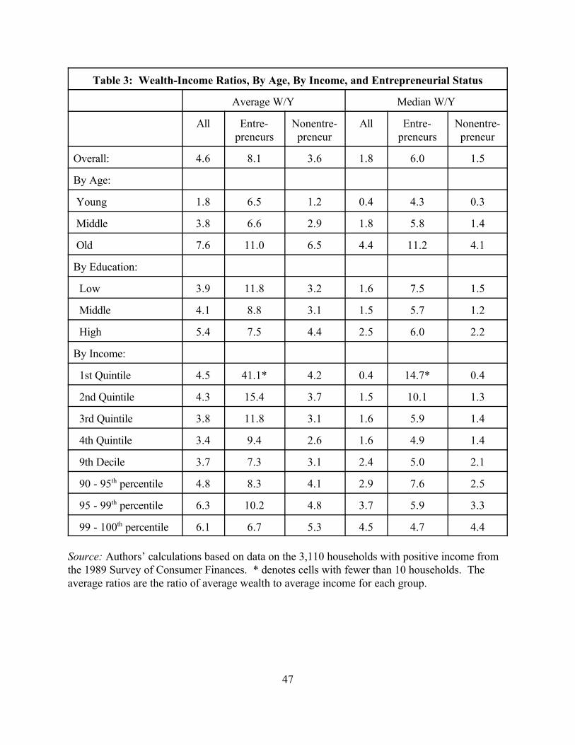
47

Table 3: Wealth-Income Ratios, By Age, By Income, and Entrepreneurial Status

Average W/Y Median W/Y

All Entre-preneurs

Nonentre-preneur

All Entre-preneurs

Nonentre-preneur

Overall: 4.6 8.1 3.6 1.8 6.0 1.5

By Age:

Young 1.8 6.5 1.2 0.4 4.3 0.3

Middle 3.8 6.6 2.9 1.8 5.8 1.4

Old 7.6 11.0 6.5 4.4 11.2 4.1

By Education:

Low 3.9 11.8 3.2 1.6 7.5 1.5

Middle 4.1 8.8 3.1 1.5 5.7 1.2

High 5.4 7.5 4.4 2.5 6.0 2.2

By Income:

1st Quintile 4.5 41.1* 4.2 0.4 14.7* 0.4

2nd Quintile 4.3 15.4 3.7 1.5 10.1 1.3

3rd Quintile 3.8 11.8 3.1 1.6 5.9 1.4

4th Quintile 3.4 9.4 2.6 1.6 4.9 1.4

9th Decile 3.7 7.3 3.1 2.4 5.0 2.1

90 - 95th percentile 4.8 8.3 4.1 2.9 7.6 2.5

95 - 99th percentile 6.3 10.2 4.8 3.7 5.9 3.3

99 - 100th percentile 6.1 6.7 5.3 4.5 4.7 4.4 Source: Authors’ calculations based on data on the 3,110 households with positive income fromthe 1989 Survey of Consumer Finances. * denotes cells with fewer than 10 households. Theaverage ratios are the ratio of average wealth to average income for each group.

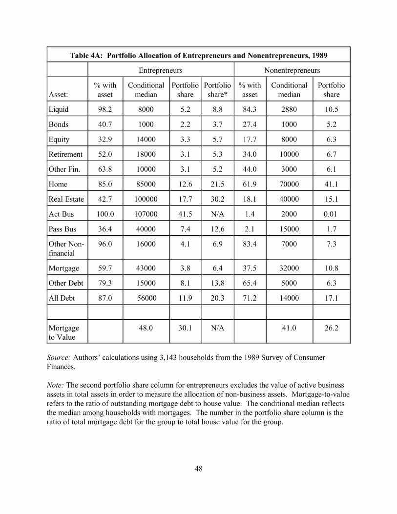
48

Table 4A: Portfolio Allocation of Entrepreneurs and Nonentrepreneurs, 1989

Entrepreneurs Nonentrepreneurs

Asset:% withasset

Conditionalmedian

Portfolioshare

Portfolioshare*

% withasset

Conditionalmedian

Portfolioshare

Liquid 98.2 8000 5.2 8.8 84.3 2880 10.5

Bonds 40.7 1000 2.2 3.7 27.4 1000 5.2

Equity 32.9 14000 3.3 5.7 17.7 8000 6.3

Retirement 52.0 18000 3.1 5.3 34.0 10000 6.7

Other Fin. 63.8 10000 3.1 5.2 44.0 3000 6.1

Home 85.0 85000 12.6 21.5 61.9 70000 41.1

Real Estate 42.7 100000 17.7 30.2 18.1 40000 15.1

Act Bus 100.0 107000 41.5 N/A 1.4 2000 0.01

Pass Bus 36.4 40000 7.4 12.6 2.1 15000 1.7

Other Non-financial

96.0 16000 4.1 6.9 83.4 7000 7.3

Mortgage 59.7 43000 3.8 6.4 37.5 32000 10.8

Other Debt 79.3 15000 8.1 13.8 65.4 5000 6.3

All Debt 87.0 56000 11.9 20.3 71.2 14000 17.1

Mortgageto Value

48.0 30.1 N/A 41.0 26.2

Source: Authors’ calculations using 3,143 households from the 1989 Survey of ConsumerFinances.

Note: The second portfolio share column for entrepreneurs excludes the value of active businessassets in total assets in order to measure the allocation of non-business assets. Mortgage-to-valuerefers to the ratio of outstanding mortgage debt to house value. The conditional median reflectsthe median among households with mortgages. The number in the portfolio share column is theratio of total mortgage debt for the group to total house value for the group.

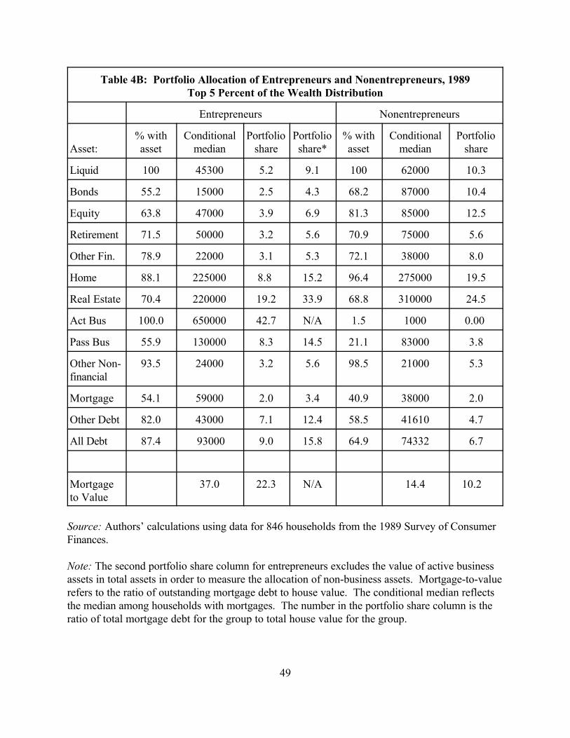
49

Table 4B: Portfolio Allocation of Entrepreneurs and Nonentrepreneurs, 1989Top 5 Percent of the Wealth Distribution

Entrepreneurs Nonentrepreneurs

Asset:% withasset

Conditionalmedian

Portfolioshare

Portfolioshare*

% withasset

Conditionalmedian

Portfolioshare

Liquid 100 45300 5.2 9.1 100 62000 10.3

Bonds 55.2 15000 2.5 4.3 68.2 87000 10.4

Equity 63.8 47000 3.9 6.9 81.3 85000 12.5

Retirement 71.5 50000 3.2 5.6 70.9 75000 5.6

Other Fin. 78.9 22000 3.1 5.3 72.1 38000 8.0

Home 88.1 225000 8.8 15.2 96.4 275000 19.5

Real Estate 70.4 220000 19.2 33.9 68.8 310000 24.5

Act Bus 100.0 650000 42.7 N/A 1.5 1000 0.00

Pass Bus 55.9 130000 8.3 14.5 21.1 83000 3.8

Other Non-financial

93.5 24000 3.2 5.6 98.5 21000 5.3

Mortgage 54.1 59000 2.0 3.4 40.9 38000 2.0

Other Debt 82.0 43000 7.1 12.4 58.5 41610 4.7

All Debt 87.4 93000 9.0 15.8 64.9 74332 6.7

Mortgageto Value

37.0 22.3 N/A 14.4 10.2

Source: Authors’ calculations using data for 846 households from the 1989 Survey of ConsumerFinances.

Note: The second portfolio share column for entrepreneurs excludes the value of active businessassets in total assets in order to measure the allocation of non-business assets. Mortgage-to-valuerefers to the ratio of outstanding mortgage debt to house value. The conditional median reflectsthe median among households with mortgages. The number in the portfolio share column is theratio of total mortgage debt for the group to total house value for the group.

50

Table 5: Changes in Portfolio Allocation by Entrepreneurial Transition, 1983 and 1989

Entrants Continuing Entrepreneurs

1983 1989 1983 1989

Asset:% withasset

Portfolioshare

% withasset

Portfolioshare

% withasset

Portfolioshare

% withasset

Portfolioshare

Liquid 99.0 8.3 99.0 4.2 100.0 3.5 95.6 3.4

Bonds 37.0 1.4 33.0 1.7 27.2 2.4 32.3 3.8

Equity 28.9 7.1 29.4 2.8 34.3 9.5 38.7 4.1

Retirement 34.2 4.0 47.9 3.8 55.8 1.8 59.7 3.0

Other Fin. 52.5 7.6 66.3 2.4 56.3 4.7 63.1 2.8

Home 76.5 37.0 82.2 22.9 93.2 15.9 96.2 11.7

Real Estate 41.2 21.6 48.5 9.8 34.8 11.9 40.2 12.5

Act Bus 0.016 0.02 100.0 45.3 100.0 41.8 100.0 47.9

Pass Bus 11.2 7.6 22.7 2.5 15.1 6.3 22.7 8.5

Other Non-financial

99.9 5.3 97.0 4.7 97.1 2.1 93.7 2.3

Mortgage 58.3 12.2 61.1 9.1 71.0 3.7 71.3 3.2

Other Debt 83.2 8.8 79.7 3.4 85.6 3.0 78.3 4.1

All Debt 89.1 21.0 83.9 12.5 89.4 6.7 89.9 7.3

Mortgageto Value

32.9 40.0 23.3 27.6

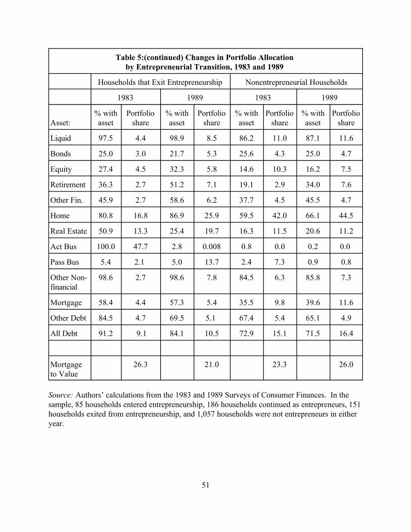
51

Table 5:(continued) Changes in Portfolio Allocation by Entrepreneurial Transition, 1983 and 1989

Households that Exit Entrepreneurship Nonentrepreneurial Households

1983 1989 1983 1989

Asset:% withasset

Portfolioshare

% withasset

Portfolioshare

% withasset

Portfolioshare

% withasset

Portfolioshare

Liquid 97.5 4.4 98.9 8.5 86.2 11.0 87.1 11.6

Bonds 25.0 3.0 21.7 5.3 25.6 4.3 25.0 4.7

Equity 27.4 4.5 32.3 5.8 14.6 10.3 16.2 7.5

Retirement 36.3 2.7 51.2 7.1 19.1 2.9 34.0 7.6

Other Fin. 45.9 2.7 58.6 6.2 37.7 4.5 45.5 4.7

Home 80.8 16.8 86.9 25.9 59.5 42.0 66.1 44.5

Real Estate 50.9 13.3 25.4 19.7 16.3 11.5 20.6 11.2

Act Bus 100.0 47.7 2.8 0.008 0.8 0.0 0.2 0.0

Pass Bus 5.4 2.1 5.0 13.7 2.4 7.3 0.9 0.8

Other Non-financial

98.6 2.7 98.6 7.8 84.5 6.3 85.8 7.3

Mortgage 58.4 4.4 57.3 5.4 35.5 9.8 39.6 11.6

Other Debt 84.5 4.7 69.5 5.1 67.4 5.4 65.1 4.9

All Debt 91.2 9.1 84.1 10.5 72.9 15.1 71.5 16.4

Mortgageto Value

26.3 21.0 23.3 26.0

Source: Authors’ calculations from the 1983 and 1989 Surveys of Consumer Finances. In thesample, 85 households entered entrepreneurship, 186 households continued as entrepreneurs, 151households exited from entrepreneurship, and 1,057 households were not entrepreneurs in eitheryear.

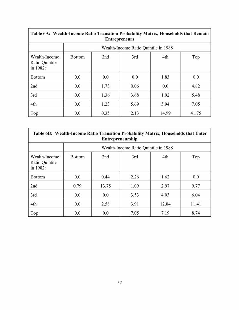
52

Table 6A: Wealth-Income Ratio Transition Probability Matrix, Households that RemainEntrepreneurs

Wealth-Income Ratio Quintile in 1988

Wealth-IncomeRatio Quintilein 1982:

Bottom 2nd 3rd 4th Top

Bottom 0.0 0.0 0.0 1.83 0.0

2nd 0.0 1.73 0.06 0.0 4.82

3rd 0.0 1.36 3.68 1.92 5.48

4th 0.0 1.23 5.69 5.94 7.05

Top 0.0 0.35 2.13 14.99 41.75

Table 6B: Wealth-Income Ratio Transition Probability Matrix, Households that EnterEntrepreneurship

Wealth-Income Ratio Quintile in 1988

Wealth-IncomeRatio Quintilein 1982:

Bottom 2nd 3rd 4th Top

Bottom 0.0 0.44 2.26 1.62 0.0

2nd 0.79 13.75 1.09 2.97 9.77

3rd 0.0 0.0 3.53 4.03 6.04

4th 0.0 2.58 3.91 12.84 11.41

Top 0.0 0.0 7.05 7.19 8.74

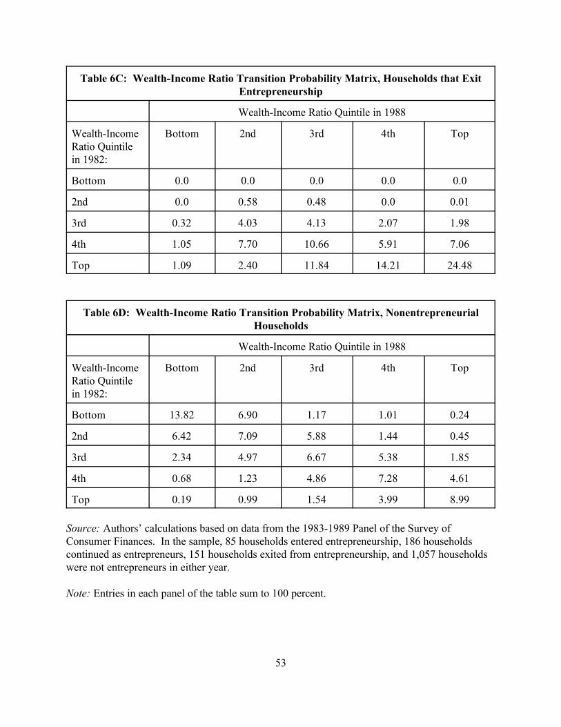
53

Table 6C: Wealth-Income Ratio Transition Probability Matrix, Households that ExitEntrepreneurship

Wealth-Income Ratio Quintile in 1988

Wealth-IncomeRatio Quintilein 1982:

Bottom 2nd 3rd 4th Top

Bottom 0.0 0.0 0.0 0.0 0.0

2nd 0.0 0.58 0.48 0.0 0.01

3rd 0.32 4.03 4.13 2.07 1.98

4th 1.05 7.70 10.66 5.91 7.06

Top 1.09 2.40 11.84 14.21 24.48

Table 6D: Wealth-Income Ratio Transition Probability Matrix, NonentrepreneurialHouseholds

Wealth-Income Ratio Quintile in 1988

Wealth-IncomeRatio Quintilein 1982:

Bottom 2nd 3rd 4th Top

Bottom 13.82 6.90 1.17 1.01 0.24

2nd 6.42 7.09 5.88 1.44 0.45

3rd 2.34 4.97 6.67 5.38 1.85

4th 0.68 1.23 4.86 7.28 4.61

Top 0.19 0.99 1.54 3.99 8.99

Source: Authors’ calculations based on data from the 1983-1989 Panel of the Survey ofConsumer Finances. In the sample, 85 households entered entrepreneurship, 186 householdscontinued as entrepreneurs, 151 households exited from entrepreneurship, and 1,057 householdswere not entrepreneurs in either year.

Note: Entries in each panel of the table sum to 100 percent.

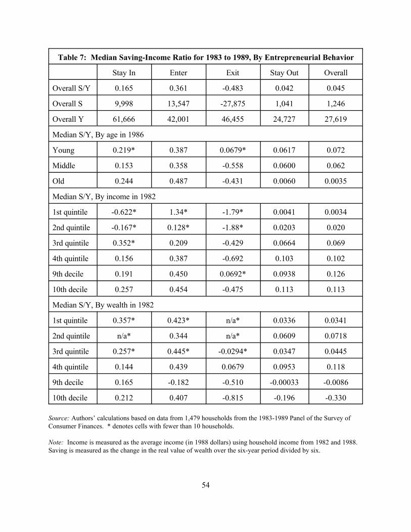
54

Table 7: Median Saving-Income Ratio for 1983 to 1989, By Entrepreneurial Behavior

Stay In Enter Exit Stay Out Overall

Overall S/Y 0.165 0.361 -0.483 0.042 0.045

Overall S 9,998 13,547 -27,875 1,041 1,246

Overall Y 61,666 42,001 46,455 24,727 27,619

Median S/Y, By age in 1986

Young 0.219* 0.387 0.0679* 0.0617 0.072

Middle 0.153 0.358 -0.558 0.0600 0.062

Old 0.244 0.487 -0.431 0.0060 0.0035

Median S/Y, By income in 1982

1st quintile -0.622* 1.34* -1.79* 0.0041 0.0034

2nd quintile -0.167* 0.128* -1.88* 0.0203 0.020

3rd quintile 0.352* 0.209 -0.429 0.0664 0.069

4th quintile 0.156 0.387 -0.692 0.103 0.102

9th decile 0.191 0.450 0.0692* 0.0938 0.126

10th decile 0.257 0.454 -0.475 0.113 0.113

Median S/Y, By wealth in 1982

1st quintile 0.357* 0.423* n/a* 0.0336 0.0341

2nd quintile n/a* 0.344 n/a* 0.0609 0.0718

3rd quintile 0.257* 0.445* -0.0294* 0.0347 0.0445

4th quintile 0.144 0.439 0.0679 0.0953 0.118

9th decile 0.165 -0.182 -0.510 -0.00033 -0.0086

10th decile 0.212 0.407 -0.815 -0.196 -0.330

Source: Authors’ calculations based on data from 1,479 households from the 1983-1989 Panel of the Survey ofConsumer Finances. * denotes cells with fewer than 10 households.

Note: Income is measured as the average income (in 1988 dollars) using household income from 1982 and 1988. Saving is measured as the change in the real value of wealth over the six-year period divided by six.

55

Table 8: Summary Statistics of Household Characteristics, By Entrepreneurial BehaviorStay In Enter Exit Stay Out Overall

MARRIED 0.82(0.39)

0.72(0.45)

0.83(0.38)

0.58(0.49)

0.61(0.49)

GOTDIVORCED

0.035(0.18)

0.075(0.26)

0.17(0.37)

0.084(0.28)

0.085(0.28)

BECAMEWIDOWED

0.0046(0.068)

0.0096(0.098)

0.031(0.17)

0.056(0.23)

0.050(0.22)

GOT MARRIED 0.035(0.18)

0.19(0.40)

0.12(0.33)

0.094(0.29)

0.098(0.30)

FAMILY SIZE 2.76(1.12)

2.62(1.01)

2.70(1.05)

2.36(1.25)

2.41(1.23)

AGE2 0.54(0.50)

0.29(0.45)

0.43(0.50)

0.32(0.47)

0.33(0.47)

AGE3 0.15(0.35)

0.15(0.36)

0.36(0.48)

0.32(0.47)

0.31(0.46)

UNEMPLOYED 0.00(0.00)

0.050(0.22)

0.00(0.00)

0.074(0.26)

0.066(0.25)

EDUC 13.67(2.74)

13.67(2.56)

13.57(2.29)

12.11(3.26)

12.33(3.22)

DEFBEN 0.26(0.44)

0.29(0.46)

0.21(0.41)

0.39(0.49)

0.37(0.48)

INHERIT 0.14(0.35)

0.031(0.17)

0.10(0.30)

0.084(0.28)

0.085(0.28)

Homeowner in1982 & 1988

0.92(0.27)

0.66(0.47)

0.68(0.47)

0.53(0.50)

0.56(0.50)

Homeowner bothyears but moved

0.16(0.36)

0.17(0.38)

0.14(0.35)

0.081(0.27)

0.092(0.29)

Renter in 1982,Owner in 1988

0.037(0.19)

0.15(0.36)

0.18(0.39)

0.14(0.34)

0.13(0.34)

Owner in 1982,Renter in 1988

0.024(0.15)

0.094(0.29)

0.11(0.31)

0.70(0.26)

0.071(0.26)

Source: The entries are the means for each sample with standard deviations in parentheses.Authors’ calculations based on data from 1,479 households from the 1983-1989 Panel of theSurvey of Consumer Finances.

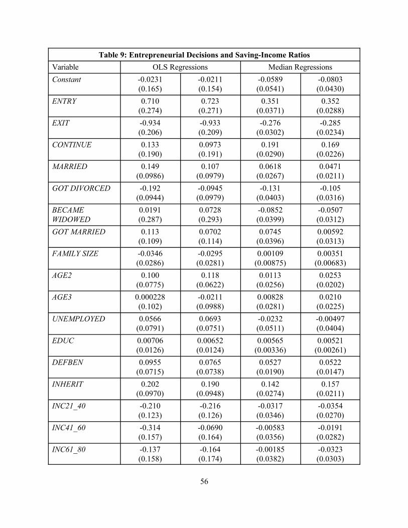
56

Table 9: Entrepreneurial Decisions and Saving-Income RatiosVariable OLS Regressions Median Regressions

Constant -0.0231(0.165)

-0.0211(0.154)

-0.0589(0.0541)

-0.0803(0.0430)

ENTRY 0.710(0.274)

0.723(0.271)

0.351(0.0371)

0.352(0.0288)

EXIT -0.934(0.206)

-0.933(0.209)

-0.276(0.0302)

-0.285(0.0234)

CONTINUE 0.133(0.190)

0.0973(0.191)

0.191(0.0290)

0.169(0.0226)

MARRIED 0.149(0.0986)

0.107(0.0979)

0.0618(0.0267)

0.0471(0.0211)

GOT DIVORCED -0.192(0.0944)

-0.0945(0.0979)

-0.131(0.0403)

-0.105(0.0316)

BECAMEWIDOWED

0.0191(0.287)

0.0728(0.293)

-0.0852(0.0399)

-0.0507(0.0312)

GOT MARRIED 0.113(0.109)

0.0702(0.114)

0.0745(0.0396)

0.00592(0.0313)

FAMILY SIZE -0.0346(0.0286)

-0.0295(0.0281)

0.00109(0.00875)

0.00351(0.00683)

AGE2 0.100(0.0775)

0.118(0.0622)

0.0113(0.0256)

0.0253(0.0202)

AGE3 0.000228(0.102)

-0.0211(0.0988)

0.00828(0.0281)

0.0210(0.0225)

UNEMPLOYED 0.0566(0.0791)

0.0693(0.0751)

-0.0232(0.0511)

-0.00497(0.0404)

EDUC 0.00706(0.0126)

0.00652(0.0124)

0.00565(0.00336)

0.00521(0.00261)

DEFBEN 0.0955(0.0715)

0.0765(0.0738)

0.0527(0.0190)

0.0522(0.0147)

INHERIT 0.202(0.0970)

0.190(0.0948)

0.142(0.0274)

0.157(0.0211)

INC21_40 -0.210(0.123)

-0.216(0.126)

-0.0317(0.0346)

-0.0354(0.0270)

INC41_60 -0.314(0.157)

-0.0690(0.164)

-0.00583(0.0356)

-0.0191(0.0282)

INC61_80 -0.137(0.158)

-0.164(0.174)

-0.00185(0.0382)

-0.0323(0.0303)

Table 9: Entrepreneurial Decisions and Saving-Income RatiosVariable OLS Regressions Median Regressions

57

INC81_90 0.00500(0.159)

0.00743(0.173)

0.0429(0.0439)

0.0236(0.0349)

INC91_95 -0.000392(0.198)

-0.0382(0.211)

0.0125(0.0506)

-0.0213(0.0398)

INC96_99 -0.0440(0.242)

-0.0476(0.256)

0.182(0.0456)

0.158(0.0364)

INC99+ 0.306(0.242)

0.319(0.246)

0.312(0.0451)

0.270(0.0360)

Homeowner in1982 & 1988

0.0993(0.0901)

0.0566(0.0215)

Homeowner bothyears but moved

-0.0806(0.0894)

-0.0591(0.0217)

Renter in 1982,Owner in 1988

0.0992(0.103)

0.195(0.0324)

Owner in 1982,Renter in 1988

-0.358(0.156)

-0.254(0.0364)

Adj. R2 0.059 0.067 0.056 0.065

Source: Estimates using panel data from the 1983-1989 Survey of Consumer Finances.

Note: Standard errors are in parentheses. Regressions use 4,434 observations, representingapproximately 1,478 households. Standard errors are multiplied by the square root of three toadjust for the replications. Income in the saving-income ratio is measured as the average income(in 1988 dollars) using household income from 1982 and 1988. Saving is measured as the changein the real value of wealth over the six-year period divided by six. OLS regressions usepopulation weights; median regressions are unweighted.

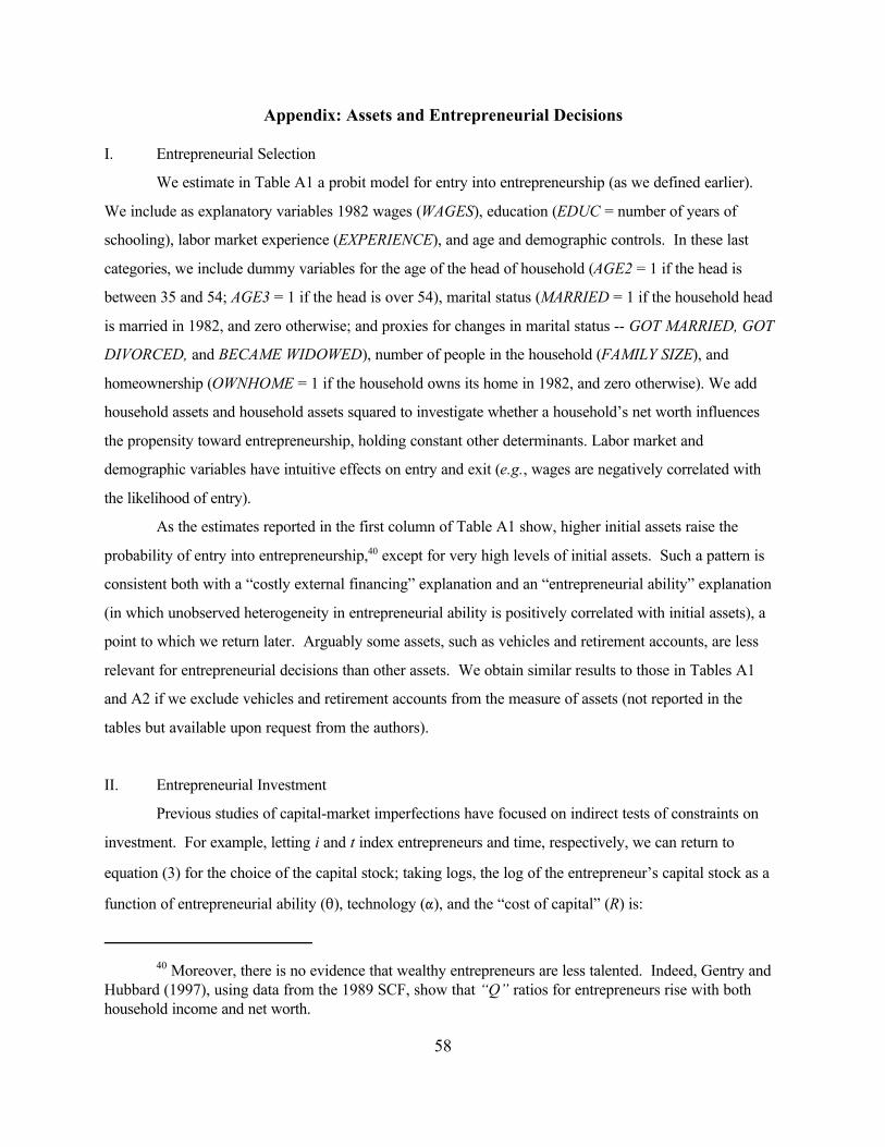
40 Moreover, there is no evidence that wealthy entrepreneurs are less talented. Indeed, Gentry andHubbard (1997), using data from the 1989 SCF, show that “Q” ratios for entrepreneurs rise with bothhousehold income and net worth.

58

Appendix: Assets and Entrepreneurial Decisions

I. Entrepreneurial Selection

We estimate in Table A1 a probit model for entry into entrepreneurship (as we defined earlier).

We include as explanatory variables 1982 wages (WAGES), education (EDUC = number of years of

schooling), labor market experience (EXPERIENCE), and age and demographic controls. In these last

categories, we include dummy variables for the age of the head of household (AGE2 = 1 if the head is

between 35 and 54; AGE3 = 1 if the head is over 54), marital status (MARRIED = 1 if the household head

is married in 1982, and zero otherwise; and proxies for changes in marital status -- GOT MARRIED, GOT

DIVORCED, and BECAME WIDOWED), number of people in the household (FAMILY SIZE), and

homeownership (OWNHOME = 1 if the household owns its home in 1982, and zero otherwise). We add

household assets and household assets squared to investigate whether a household’s net worth influences

the propensity toward entrepreneurship, holding constant other determinants. Labor market and

demographic variables have intuitive effects on entry and exit (e.g., wages are negatively correlated with

the likelihood of entry).

As the estimates reported in the first column of Table A1 show, higher initial assets raise the

probability of entry into entrepreneurship,40 except for very high levels of initial assets. Such a pattern is

consistent both with a “costly external financing” explanation and an “entrepreneurial ability” explanation

(in which unobserved heterogeneity in entrepreneurial ability is positively correlated with initial assets), a

point to which we return later. Arguably some assets, such as vehicles and retirement accounts, are less

relevant for entrepreneurial decisions than other assets. We obtain similar results to those in Tables A1

and A2 if we exclude vehicles and retirement accounts from the measure of assets (not reported in the

tables but available upon request from the authors).

II. Entrepreneurial Investment

Previous studies of capital-market imperfections have focused on indirect tests of constraints on

investment. For example, letting i and t index entrepreneurs and time, respectively, we can return to

equation (3) for the choice of the capital stock; taking logs, the log of the entrepreneur’s capital stock as a

function of entrepreneurial ability (2), technology ("), and the “cost of capital” (R) is:

59

, (A1)( )( ) ( )( ) ( )( )l l l lnkit n i n n Rit it= − + − − −∧

+1 1 1 1 1 1/ / /α θ α α α ω

where , and T is a white-noise optimization error.R Rak

∧= + +

Ø Ø' After controlling for 2 ,", and , there should be no predictive power for the capital stock ofR

beginning-of-period nonbusiness assets, an. That is, if we add nonbusiness assets as a regressor in equation

(A1), its estimated coefficient should be zero under the null hypothesis of perfect capital markets.

Unfortunately, cross-sectional tests using the level of assets across entrepreneurs are likely to confound the

effects of unobserved talent and assets. A positive correlation between unobserved talent and assets would

upwardly bias the estimated coefficient on nonbusiness assets in the regression for the capital stock. These

biases would be less severe with panel data on investment flows; however, such data are not available in

the SCF.

It is possible, however, to examine the link between net worth and investment by studying the

relationship between net worth and entrepreneurial earnings. Under the null hypothesis of perfect markets,

one can substitute the optimal capital stock for k from equation (A1) into the definition of entrepreneurial

earnings in equation (1), so that yit = 2i 1/(1-") (" / it) "/(1-") ,it , orR

Rnyit = (1/(1 - ")) Rn2i + (" /(1-"))Rn" + (" /(1-"))Rn it + Rn,it . (A2)R

Here, one can test whether predetermined assets affect entrepreneurial earnings. First-differencing

equation (A2) removes the entrepreneurial-ability term. If one adds an initial nonbusiness assets variable to

that model, its estimated coefficient should be zero under the null hypothesis of perfect capital markets.

The model of costly external financing presented earlier suggests an alternative role for assets and

internally generated funds. Higher initial assets decrease the external financing premium, reducing the cost

of capital and increasing business investment, k, and business income, y.

Using data on continuing entrepreneurs, we report estimates for two specifications of equation (A2)

in Appendix Table A2. In both, we include household variables (marital status, number of children, age,

and education), and business industry dummy variables. We first estimate equation (A2) in log differences;

because some observations have zero or negative business income in one or both years, we also estimate

(A2) in level differences. In the change in levels specification, the estimated coefficient on initial

nonbusiness assets is marginally statistically significantly different from zero, inconsistent with the null

hypothesis of frictionless financing for entrepreneurs.

60

Table A1: Assets and Entrepreneurial EntryVariable Probit Coefficients Marginal EffectsConstant -2.65

(0.480)MARRIED 0.512

(0.369)0.0389

(0.0241)GOT MARRIED 0.776

(0.380)0.105

(0.0687)GOT DIVORCED -0.273

(0.330)-0.0177(0.0171)

FAMILY SIZE -0.0948(0.0826)

-0.00748(0.00618)

AGE2 -0.482(0.203)

-0.0335(0.0117)

AGE3 -0.693(0.254)

-0.0435(0.0158)

OWNHOME 0.531(0.220)

0.0392(0.0172)

EXPERIENCE 0.0117(0.00669)

0.000925(0.000524)

EDUC 0.0509(0.0301)

0.00401(0.00249)

“WAGES” -0.000000905(0.00000244)

-7.14e-8 (1.96e-7)

ASSETS 0.00000118(0.000000491)

9.29e-8(3.98e-8)

ASSETS2 -2.68e-13(1.38e-13)

-2.11e-14(1.10e-14)

Pseudo R2 0.13

Source: Probit estimates using panel data from the 1983-1989 Survey of Consumer Finances.

Note: Standard errors are in parentheses. The regression uses 3,434 observations, representingapproximately 1,145 households. The standard errors are multiplied by the square root of three to adjustfor replicated data. “WAGES”equals the sum of 1982 wage and business income. None of the householdsthat “Became widowed” entered entrepreneurship. Marginal effects are calculated at the means of thevariables. For discrete variables, the marginal effect is the effect of changing the value of the variable fromzero to one.

61

Table A2: Assets and Business Income Growth

Variable Change in Log of Business Income Change in Level of Business Income($000)

Constant -5.01(5.42)

3.88(122.3)

MARRIED -0.952(0.585)

3.56(33.4)

GOT MARRIED -0.639(0.654)

182.9(153.8)

GOT DIVORCED -4.93(0.736)

-155.8(118.9)

BECAME WIDOWED 1.17(1.25)

85.4(156.3)

FAMILY SIZE -0.180(0.243)

-13.8(15.7)

AGE2 -0.431(0.608)

-51.4(38.6)

AGE3 -0.146(0.857)

-70.5(68.7)

EDUC 0.145(0.111)

-0.276(4.95)

DEFBEN -0.779(0.431)

-5.44(40.0)

Log of other assets in1982

0.390(0.346)

Other assets in 1982($000)

0.0694(0.0470)

Other assets in 1982,squared ($000)

-5.99e-10(1.17e-09)

Adj. R2 0.47 0.14

Source: OLS estimates using panel data from the 1983-1989 Survey of Consumer Finances.

Note: Standard errors are in parentheses. Regressions include dummy variables for the business industry. The sample includes only households that were entrepreneurs in both years. The log regression uses 240observations, representing approximately 80 households. The level regression uses 556 observations, orapproximately 185 households. The standard errors are multiplied by the square root of three to adjust forreplications in the data.