Entanglement: from its mathematical description to its ... · Entanglement: from its mathematical...
120
Entanglement: from its mathematical description to its experimental observation Daniel Cavalcanti Santos Director: Antonio Ac´ ın Dal Maschio Tutor: Jos´ e Ignacio Latorre Tesis presentada para optar al grado de doctor por el programa de f´ ısica avanzada del Departament d’Estructura i Constituents de la Mat` eria de la Universitat de Barcelona. Bienio: 2006/2007. Barcelona, May, 2008.
Transcript of Entanglement: from its mathematical description to its ... · Entanglement: from its mathematical...

Entanglement: from its mathematical description
to its experimental observation
Daniel Cavalcanti Santos
Director: Antonio Acın Dal MaschioTutor: Jose Ignacio Latorre
Tesis presentada para optar al grado de doctor por el programa de fısicaavanzada del Departament d’Estructura i Constituents de la Materia de la
Universitat de Barcelona.Bienio: 2006/2007.
Barcelona, May, 2008.


Acknowledgments
Of course it will be difficult to put everybody i should thank in thisacknowledgment. So let me say THANKS for everybody who helped meto get here, in BCN, defending this PhD thesis. Uff....now I didn’t missanybody! But ok...let me make some specially thank some people who helpedme a lot during all these years .
I must start by thanking Toni, first of all for being a friend. We alwayshad a good time together, in ICFO, having dinners, beers, playing football,.... But of course i have to say that he is also a really good supervisor:relaxed enough for making light work (hmmm?!!!!), but at the same timealways pushing me with a lot of good ideas. Ah, and i can’t forget to thankhim for the hitchhiking during the flats change!
The second person i must thank is Flavia. Leaving one year far away wasnot easy, but i am sure it was as easy as possible!!! Thanks for coming, forwaking up with me everyday (this is not easy, hm?!!!), for making “moussede chocolate” (apesar de me por pra bater clara em neve ;)), for listen to metalking about entanglement, ...for so many things that it is impossible to putall of them here. Thanks thanks thanks thanks....smacccchhhh!!!!
A BIG thanks for my family. Um beij ao pra vovo Dea, vovo Emis, MamaeMalina e pro Fulustrico The support they always gave me is amazing.
A special thank for Terra for being so open-minded and letting me scapeto BCN!
I also must say that I am very luck to work in this group. Nothing isbetter than working besides friends! I have been learning so many thingswith Maf, Artur, Stefano, Ale, Miguel, Joonwoo, Giuseppe, and Leandro!Thank you guys! But specially, thanks: Ale, for saving me in Pisa. Man, iwill never forget your face, at 4am, saying “el doctor dijo que tendras queoperar ahora mismo!!!” Que putada! Maf, for all the good time we hadtogether (quanta festa heim!!!). Brigadao! Miguel and Stefano for the goodemails (please, keep thinking that a good joke is better than a PRL).
Let me also thank Simone Montangero for the help in Pisa. I think hedoesn’t know, but his friend appeared in a crucial moment!!!
I am very thankful for all my collaborators: Terra, Leandro (Ciolleti),Marcelo Franca, Fernando, Ze Jr, Ze Pai, Xubaca, Franklin, Leandro (Aolita),Planet, Alejo, Luiz, Vlatko, Christian, Monken, Pablo, Olavo, Sebastiao,Toni, Ale Ferraro, and Artur.

2
Finally, before start talking about entanglement many thanks also for......Carlos (for being noisy) and Irene (for being noiseless)....Leandro, Planet, Ale, and Sol for bikes and bikes....Clara for correcting my spanish....Benasque Center for Sciences for organizing the best conference ever....A. Buchleitner’s group for the very nice week in Freiburg....C. Monken and Mario Sergio for pushing me to come to BCN....the good weather of BCN.THANK YOU ALL!

3
Abstract
Entanglement is the main quantum property that makes quantum infor-mation protocols more powerful than any classical counterpart. Moreover,understanding entanglement allows a better comprehension of physical phe-nomena in the fields of condensed matter, statistical physics, and quantumoptics among others.
The open questions on entanglement range from fundamental to practicalissues. How to characterize the entanglement of quantum systems? Whatis entanglement useful for? What is the relation between entanglement andother physical phenomena? These are some open questions we are faced withnowadays.
This thesis contains several original results in this field. Some of theaddressed questions rely on the mathematical description of entanglementwhile others on its description in some physical systems. More specifically,
(i) it will be shown a relation between two quantifiers of entanglement,the generalized robustness and the geometric measure of entanglement ;
(ii) the entanglement of superpositions will be generalized to the multi-partite case and to several entanglement quantifiers;
(iii) a recently proposed Bell inequality for continuous-variable (CV) sys-tems will be used to extend, for the CV scenario, the Peres’ conjecture thatbound entangled states admit a description in terms of hidden variables.
(iv) a proposal to probe the geometry of the set of separable states willbe made. This approach is able to find singularities in the border of this set,and those are reflected in the entanglement properties of condensed matter,atomic, and photonic systems. An experiment involving entangled photonscoming from parametric down conversion will be described to illustrate thetheoretical results;
(v) the decay of entanglement of generalized N -particle GHZ states inter-acting with independent reservoirs will be investigated. Scaling laws for thedecay of entanglement and for its finite-time extinction (sudden death) arederived for different types of reservoirs. The latter is found to increase withthe number of particles. However, entanglement becomes arbitrarily small,and therefore useless as a resource, much before it completely disappears,around a time which is inversely proportional to the number of particles.The decay of multi-particle GHZ states will be shown to generate boundentangled states;

4
(vi) and finally, the entanglement properties of particles in a non-interactingFermi gas are studied. Since there is no interaction among the particles, thisentanglement comes solely from the statistical properties of the particles. Itwill be shown how the way we detect the particles changes their entanglementproperties. Additionally a realistic proposal to convert identical particle en-tanglement of fermions in a quantum well into useful photonic entanglementwill be given.

5
List of Publications
1. Scaling Laws for the decay of multiqubit entanglement.L. Aolita, R. Chaves, D. Cavalcanti, A. Acın, and L. Davidovich.Physical Review Letters 100, 080501 (2008).
2. Thermal bound entanglement in macroscopic systems and area law.A. Ferraro, D. Cavalcanti, A. Garcıa-Saez, and A. Acın.Physical Review Letters 100, 080502 (2008).
3. Area laws and entanglement distillability of thermal states.D. Cavalcanti, A. Ferraro, A. Garcıa-Saez, and A. Acın.Proceedings of the “Entanglement and Many-body Systems” Confer-ence, Pisa May 2008.
4. Distillable entanglement and area laws in spin and harmonic-oscillatorsystems.D. Cavalcanti, A. Ferraro, A. Garcıa-Saez, and A. Acın.Submitted to Physical Review A (2008) - preprint available as arXiv:0705.3762.
5. Geometrically induced singular behavior of entanglement.D. Cavalcanti, P.L. Saldanha, O. Cosme, F.G.S.L. Brandao, C.H. Monken,S. Padua, M. F. Santos, and M. O. Terra Cunha.Submitted to Physical Review Letters (2008) - preprint available asarXiv:0709.0301.
6. Non-locality and Partial Transposition for Continuous-Variable Sys-tems.A. Salles, D. Cavalcanti and A. Acın.Submitted to Physical Review Letters (2008) - preprint available asarXiv:0804.4703.
7. Multipartite entanglement of superpositions.D. Cavalcanti, M. O. Terra Cunha, and A. Acın.Physical Review A 76, 042329 (2007).
8. Useful entanglement from the Pauli principle.D. Cavalcanti, L. M. Moreira, F. M. Matinaga, M.O. Terra Cunha, andM.F. Santos.Phys. Rev. B 76, 113304 (2007).

6
9. Connecting the generalized robustness and the geometric measure ofentanglement.D. Cavalcanti.Physical Review A 73, 044302 (2006).
10. Estimating entanglement of unknown states.D. Cavalcanti and M. O. Terra Cunha.Applied Physics Letters 89, 084102 (2006).
11. Entanglement versus energy in the entanglement transfer problem.D. Cavalcanti, J. G. Oliveira Jr, J. G. Peixoto de Faria, M.O. TerraCunha, and M.F. Santos.Physical Review A 74, 042328, (2006).
12. Entanglement quantifiers, entanglement crossover, and phase transi-tions.D. Cavalcanti, F.G.S.L. Brandao, and M.O. Terra Cunha.New Journal of Physics 8, 260 (2006).
13. Are all maximally entangled states pure?D. Cavalcanti, F.G.S.L. Brandao, and M.O. Terra Cunha.Physical Review A 72, 040303(R) (2005).
14. Increasing identical particle entanglement by fuzzy measurements.D. Cavalcanti, M.F. Santos, M. O. Terra Cunha, C. Lunkes, and V.Vedral.Physical Review A 72, 062307 (2005).
15. Tomographic characterization of three-qubit pure states using only two-qubit detectors.D. Cavalcanti, L.M. Cioletti, and M.O. Terra Cunha.Physical Review A 71, 034301 (2005).

Contents
Aknowlegments 1
Abstract 3
List of Publications 5
1 Introduction 11
1.1 Motivation . . . . . . . . . . . . . . . . . . . . . . . . . . . . . 121.2 Contributions . . . . . . . . . . . . . . . . . . . . . . . . . . . 141.3 Overview . . . . . . . . . . . . . . . . . . . . . . . . . . . . . . 17
2 Background 19
2.1 What is entanglement? . . . . . . . . . . . . . . . . . . . . . . 192.2 How to detect entanglement? . . . . . . . . . . . . . . . . . . 212.3 How to quantify entanglement? . . . . . . . . . . . . . . . . . 24
3 Connecting the Geometric Measure and the Generalized Ro-
bustness of Entanglement 31
3.1 Relating Rg and EGME to entanglement witnesses. . . . . . . . 313.2 EGME as a lower bound for Rg . . . . . . . . . . . . . . . . . . 323.3 Examples . . . . . . . . . . . . . . . . . . . . . . . . . . . . . 333.4 Concluding remarks . . . . . . . . . . . . . . . . . . . . . . . . 35
4 Multipartite entanglement of superpositions 37
4.1 Dealing with the witnessed entanglement . . . . . . . . . . . . 374.2 Are these relations tight? . . . . . . . . . . . . . . . . . . . . . 394.3 Concluding remarks . . . . . . . . . . . . . . . . . . . . . . . . 41
5 Non-locality and partial transposition for continuous variable
systems 43
5.1 The CFRD inequality . . . . . . . . . . . . . . . . . . . . . . . 455.2 SV criterion . . . . . . . . . . . . . . . . . . . . . . . . . . . . 46
7

8 CONTENTS
5.3 Nonlocality implies NPT . . . . . . . . . . . . . . . . . . . . . 47
5.4 Non-orthogonal quadratures . . . . . . . . . . . . . . . . . . . 49
5.5 Relevance of the CFRD inequality . . . . . . . . . . . . . . . . 50
5.6 Concuding remarks . . . . . . . . . . . . . . . . . . . . . . . . 51
6 Geometrically induced singular behavior of entanglement 53
6.1 The random robustness as a geometric microscope . . . . . . . 54
6.2 Where do these singularities appear? . . . . . . . . . . . . . . 56
6.2.1 Entanglement swapping . . . . . . . . . . . . . . . . . 56
6.2.2 Bit-flip noisy channel . . . . . . . . . . . . . . . . . . . 56
6.2.3 Spin systems . . . . . . . . . . . . . . . . . . . . . . . 58
6.3 Concluding remarks . . . . . . . . . . . . . . . . . . . . . . . . 58
7 Scaling laws for the decay of multiqubit entanglement 63
7.1 Decoherence models . . . . . . . . . . . . . . . . . . . . . . . . 64
7.1.1 Generalized Amplitude Damping Channel . . . . . . . 65
7.1.2 Depolarizing Channel . . . . . . . . . . . . . . . . . . . 65
7.1.3 Phase Damping Channel . . . . . . . . . . . . . . . . . 66
7.2 Entanglement sudden death . . . . . . . . . . . . . . . . . . . 66
7.3 The environment as a creator of bound entanglement . . . . . 69
7.4 Does the time of ESD really matter for large N? . . . . . . . . 69
7.5 Concluding remarks . . . . . . . . . . . . . . . . . . . . . . . . 71
8 Identical particle entanglement in Fermionic systems 73
8.1 Non-interacting Fermi gas . . . . . . . . . . . . . . . . . . . . 74
8.1.1 Perfect detection . . . . . . . . . . . . . . . . . . . . . 74
8.1.2 Imperfect detection . . . . . . . . . . . . . . . . . . . . 76
8.2 Useful entanglement from the Pauli principle . . . . . . . . . . 78
8.2.1 Selection rules . . . . . . . . . . . . . . . . . . . . . . . 79
8.2.2 From fermions to photons . . . . . . . . . . . . . . . . 80
8.2.3 Some imperfections . . . . . . . . . . . . . . . . . . . . 82
8.3 Concluding remarks . . . . . . . . . . . . . . . . . . . . . . . . 84
9 Conclusions and Perspectives 87
A Multipartite entanglement 89
B RkR as a detector of singularities in Sk 91
C Experimental Setup 93

CONTENTS 9
D Full separability of GHZ states under the Amplitude Damp-
ing Channel 95
E Resumen 97
E.1 Introduccıon a la teorıa del entrelazamiento . . . . . . . . . . 100E.1.1 Definiciones . . . . . . . . . . . . . . . . . . . . . . . . 100E.1.2 Detectando el entrelazamiento . . . . . . . . . . . . . . 101E.1.3 Cuantificando el entrelazamiento . . . . . . . . . . . . 102
E.2 Contribuciones . . . . . . . . . . . . . . . . . . . . . . . . . . 103

10 CONTENTS

Chapter 1
Introduction
Quantum Mechanics was born as a framework to describe physical phe-nomena at the atomic level. Amazingly successful, this theory was rapidlyapplied to a lot of scenarios such as atomic emission, particle scattering, andradiation-matter interaction [ER85, FLS65].
The first strong criticism to quantum theory came with the Einstein,Podolsky and Rosen’s (EPR) paper “Can quantum-mechanical descriptionof the physical reality be considered complete?” [EPR35]. These authors rec-ognized that, although quantum theory could catch many physical effects,it allowed weird predictions such as instantaneous actions at distance. Inthe essence of the EPR argument was the use of what is nowadays calledan entangled state. Motivated by EPR, Schodinger was the one who firstdiscussed the fact that some composite quantum systems can be better un-derstood if we look at them as a whole, instead of addressing their partsseparately [Sch35].
Many years passed until J. Bell put all this discussion in more solidgrounds. Accepting the notion of local realism adopted by EPR, Bell devel-oped his famous inequality involving statistics of measurements on compositequantum systems [Bel87]. From that point on, the local realism debate couldgo to the labs. Some time later the first experimental tests of Bell inequalitiesstarted to appear [FC72, FT76, AGG81, ADG82] and confirm the non-localaspect of quantum mechanics. As unentangled states (also called separablestates) can never violate a Bell inequality, the experimental violation of Bellinequalities can be seen as the first observation of entanglement [Ter00].
Up to the 90’s the debate on separability was played mostly in a funda-mental level, relying in the grounds of Quantum Mechanics. It was only withthe appearance of the first tasks on Quantum Communication and QuantumComputation that the term “entanglement” got the status of “the resource”capable of providing us advantageous methods over classical information pro-
11

12 INTRODUCTION
cessing [NC00, BEZ00]. In 1991, it was described a Cryptographic protocolentirely based on entanglement [Eke91]. However, at that time, the commu-nity already knew that without entanglement the same goal could be reached[BB84, BBD92]. Perhaps the turning point on the theory of entanglementwas the discovery of Quantum Teleportation [BBC+93] . At that moment itbecame completely clear the role of entanglement in practical tasks.
From that point on entanglement theory took its own road, being rec-ognized as a discipline itself inside Quantum Information. Among the maingoals of entanglement theory are the development of a mathematical frame-work able to describe this issue, the search for applications of entanglement,the study of the role it plays in natural physical phenomena, and, comingback to fundamental problems, its importance in the foundations of Quan-tum Mechanics. Nowadays the literature on entanglement is amazingly big.The purpose of this thesis is not to give the reader a survey on this topic,but, instead, to contribute to the knowledge of this field. More appropri-ate reviews on entanglement are found in Refs. [HHHH07, AFOV07, PV05,Bru02, Ter02, PV98, Ver02, Eis01, EP03].
1.1 Motivation
As commented before the open questions in this field range from themathematical description to practical applications. Among all these facetsof entanglement I will try to give here a small flavor of those which motivatedme more during my PhD.
Although the mathematical definition of entanglement is relatively sim-ple, the task of deciding if a general state is entangled is incredibly difficult[Ter02, HHHH07]1. Developing techniques to attack this problem is one ofthe major goals of entanglement theory. A step further of “just” knowingwhether a state is entangled is to know how much entangled it is. Followingthis vein, entanglement quantifiers are a set of rules one applies to a quan-tum state in order to estimate its amount of entanglement [PV98]. Behindthe initial attempts to quantify entanglement was the idea of quantifyinghow useful a quantum state is to perform some task [BBP+96, BDSW96].This is a very promising way of defining entanglement quantifiers, but itcertainly depends on the task one is dealing with. A more axiomatic roadis just to define a set of properties an entanglement quantifier must satisfy,without wondering whether the quantifier itself carries a physical meaning[Vid00, VPRK97]. Finally, another approach frequently followed is to quan-
1In technical terms it is said that the problem of determining if a general state isentangled is NP-hard [Gur03].

1.1. MOTIVATION 13
tify entanglement using geometric ideas. We can organize quantum statesin mathematical sets, and define distances on these sets. The amount ofentanglement of a given state can be quantified, in this way, by the distancebetween this state and the set of unentangled states [VPRK97, VP98]. Thenumber of proposed entanglement quantifiers is huge, and understanding theproperties of each quantifier and the information they bring is an importantbranch of entanglement theory. In this sense, getting relations among theexisting quantifiers could help us to get a better understanding on how toorder quantum states in terms of their entanglement content.
With the development of entanglement theory it started to be possibleto connect this issue to other fields of physics. For instance, the study ofentanglement in realistic models has allowed us to get a deeper understandingof several phenomena in condensed matter, atomic and photonic systems[RMH01, LBMW03, KWN+07, AFOV07]. Practical questions concern whichkinds of interactions allow the production of entanglement, how it behavesunder specific unitary evolution and how is entanglement affected by thepresence of noisy environments.
Following the last point, it is essential to understand how entanglementbehaves in realistic situations where unavoidable errors in the preparationof states and unwanted interactions during the post-processing are present.Many studies linking entanglement and decoherence have appeared so far[Dio03, DH04, YE04, YE06, YE07, SMDZ07, Ter07, AJ07], but some funda-mental questions are still to be answered. One of them concerns the behaviorof multiparticle entanglement under decoherence processes [SK02, CMB04,DB04, HDB05]. From a theoretical point of view, understanding this prob-lem would give us a better understanding on the appearance of classicalitywhen increasing the system’s size. From a practical point of view, this issue iscrucial since the speed-up gained when using quantum-mechanical systems,instead of classical ones, for information processing is specially relevant inthe limit of large systems.
Finally, most of the theory of entanglement was constructed in the sce-nario of distinguishable particles. In this case one identifies (labels) thesubsystems and then defines what is a local, or individual, operation. Whendealing with identical particles the idea of entanglement becomes much sub-tler: in an identical particle scenario labeling the subsystems makes no senseanymore and then talking about local operations is misleading. Anotherproblem concerning identical particles is that entanglement “comes for free”in this case. Two fermions in the same location get spin entangled (in asinglet state) just because they obey the fermionic statistics. It is then notclear, and actually controversial, how to describe this kind of quantum cor-relations, if they are useful for quantum information processing, or even if
14 INTRODUCTION
we should call them “entanglement” [ESBL04, GM04] .
1.2 Contributions
Let me briefly comment on some of the ideas that I, together with col-laborators, developed to get a better understanding of entanglement.
Geometric Measure vs. the Robustness of Entanglement.
As already commented, many are the entanglement quantifiers proposedup to now. Finding relations between them can help us to classify them, andget a better understanding on the information they give us. I have found arelation between two standard quantifiers, the Geometric Measure (EGME)and the Generalized Robustness of Entanglement (Rg). While the first has aclear geometrical meaning as a distance between an entangled states and theset of separable states, the latter was proposed as a measure of how muchnoise a state can tolerate before it looses its entanglement.
It follows from their definition that Rg is always larger than or equal toEGME. I will show a better lower bound to Rg based only on the purity ofthe quantum state and its maximal overlap to a separable state. As we willsee it is possible to express this lower bound in terms of EGME. I will finallyidentify cases where this bound is tight.
Multipartite entanglement of superpositions.
Given two pure states |Ψ〉 and |Φ〉, how is the entanglement of the super-position state a |Ψ〉+b |Φ〉 related to the entanglement of the constituents |Ψ〉and |Φ〉? This question was first addressed by Linden, Popescu and Smolin,who gave upper bounds to the entanglement of the superposed state in termsof the entanglement of the former states [LPS06].
M. Terra Cunha, A. Acın and I have considered a possible generalizationof the Linden, Popescu and Smolin’s result to the multipartite scenario: anupper bound to the multipartite entanglement of a superposition was givenin terms of the entanglement of the superposed states and the superpositioncoefficients. We have proven that this bound is tight for a class of statescomposed by an arbitrary number of qubits. Our results also extend the en-tanglement of superpositions to a large family of quantifiers which includesthe negativity, the robustness of entanglement, and the best separable ap-proximation measure.
1.2. CONTRIBUTIONS 15
Bound entanglement and Bell violation in a continuous-variable
scenario.
Guided by the similarities between the processes of entanglement distilla-tion [BDSW96] and revealing hidden non-locality [Pop95, Per96a], A. Peresconjectured that all undistillable states2 satisfy Bell inequalities. This con-jecture has been confirmed only in the scenario where N individuals applyjust two measurement settings of binary outcomes.
Recently a new Bell inequality has appeared which can be applied to un-bounded operators, i.e. it works in a continuous-variable scenario [CFRD07].Using this new Bell inequality we will see that it is possible to extend Peresconjecture to the CV scenario, and prove that all states having a positivepartial transposition satisfy this inequality3. These results were found incollaboration with A. Salles and A. Acın.
Shining light on the geometry of entanglement.
The set of quantum states is convex and closed: convex combinations ofquantum states are also quantum states. The set of separable states formsa subset, which is again convex and closed. Apart from these features thatfollow directly from the definition of quantum and separable states [BZ06],subtler questions arise when considering these states. How to characterizethe shape or the volume of these sets and to determine whether they haveany influence on directly measurable quantities are some of these queries.
In collaboration with M. Terra Cunha, M. F. Santos, F. Brandao, P. Lima,O. Cosme, S. Padua, and C. Monken I proposed a method to investigate theshape of the set of separable states through an entanglement quantifier calledrandom robustness of entanglement. This quantifier serves as a “microscope”to probe the boundary of the set of separable states. Moreover this inves-tigation can be done experimentally, what allows to get information on theshape of the set of different entangled states in real experiments. We imple-mented this method in a photonic experiment and found singularities in theshape of the separable states in the two-qubit case. As a consequence, sin-gularities appear in the quantum correlations a system presents. I will alsoshow that this phenomenon appears naturally in physical processes like theentanglement transfer problem, spin systems under varying magnetic fields,and decoherence processes.
2The concept of entanglement distillation will be discussed later.3All states having positive partial transposition are undistillable [HHH98], while the
opposite is not known.

16 INTRODUCTION
Mutipartite Entanglement vs. Decoherence.
In the real world we never have a pure quantum state. Due to unavoidableerrors in the preparation of states or noise in their postprocessing we alwaysdeal with mixed states. Entanglement is very fragile to these noisy processesand this is certainly the main obstacle to real applications on QuantumCommunication and Computation. On the other hand, the phenomenonof coherence loss, or decoherence, is in the core of the quantum-classicaltransition [Zur03]. So, understanding how quantum systems behave underthe presence of noise is a fascinating challenge both from a practical and afundamental perspective.
With L. Aolita, R. Chaves, L. Davidovich, and A. Acın, I have addressedthis point and investigated the decay of entanglement of a representativefamily of states, namely unbalanced GHZ states consisting of an arbitrarynumber of particles. Different types of reservoirs interacting independentlywith each subsystem were considered and scaling laws for the decay of en-tanglement and for its finite-time extinction were found. The latter increaseswith the number of particles. However, entanglement becomes arbitrarilysmall, and therefore useless as a resource, much before it completely dis-appears, around a time which is inversely proportional to the number ofparticles. It was also shown that the decay of multi-particle GHZ states cangenerate bound entangled states.
Is identical-particle entanglement useful?
Suppose a gas of non-interacting fermions at zero temperature. If wepick up two fermions from this gas, are them spin-entangled? I have studiedthis question together with M. F. Santos, M. Terra Cunha, C. Lunkes, andV. Vedral, and showed that its answer depends not only on the distancebetween the particles but also on the way (the detector) we pick them. Wefirst considered an ideal measurement apparatus and defined operators thatdetect the symmetry of the spatial and spin part of the density matrix asa function of particle distance. Then, moving to realistic devices that canonly detect the position of the particle to within a certain spread, it wassurprisingly found that the entanglement between particles increases withthe broadening of detection.
In this context we also considered the problem of using this identicalparticle entanglement. For this aim, L. Malard and F. Matinaga joined usto report on a scheme to extract entanglement from semiconductor quan-tum wells. Two independent photons excite non-interacting electrons in thesemiconductor. As the electrons relax to the bottom of the conduction band,

1.3. OVERVIEW 17
the Pauli exclusion principle forces the appearance of quantum correlationsbetween them. I will show that, after the electron-hole recombination, thiscorrelation is transferred to the emitted photons as entanglement in polariza-tion, which can be further used for quantum information tasks. We can thenconclude that identical particle entanglement is indeed useful for quantuminformation processing!
1.3 Overview
I will start this thesis by reviewing the existing ideas needed to the deriva-tion of the thesis’ results. They consist on basic concepts on entanglementtheory and are given here for the sake of completeness. In the remainingchapters I will expose some of the original results I developed during myPhD.
The next three chapters are more related to the mathematical formalismof entanglement theory: chapter 2 shows a connection between two entangle-ment quantifiers, chapter 3 discusses the problem of the entanglement of su-perpositions, and chapter 4 focuses on the relation between entanglement andviolation of Bell inequalities. Chapter 5 deals with a mathematical problemas well, the geometry of entanglement, but also aims at finding consequencesof it in physical phenomena. A photonic experiment was implemented toillustrate our achievements on this subject.
The following chapters are related to the characterization of entanglementin specific physical processes. Chapter 6 describes how the entanglement ofan important family of multiparticle system changes in the presence of noise.Chapter 7 discusses the entanglement properties of degenerate Fermi gasesand how the way we observe this system influences the entanglement we de-tect. Moreover I consider an exemplary system, a semiconductor quantumwell, to show that the Pauli principle can be used to create useful entangle-ment. Finally I will draw some conclusions in the last chapter and point outfuture directions that could be followed towards a better understanding ofentanglement.


Chapter 2
Background
In this chapter I will briefly review the concepts used in the developmentof the ideas presented in the next chapters. The goal is not to give a broadoverview on each of the addressed topic. Thus, many important results onentanglement will be skipped here. The purpose of this chapter is to providethe reader a self-contained text and also of finding some useful references.Those who are already familiar with entanglement theory can skip this partof the thesis. More complete reviews on entanglement can be found in Refs.[HHHH07, AFOV07, PV05, Bru02, Ter02, PV98, Ver02, Eis01, EP03].
2.1 What is entanglement?
Quantum states are described by semi-definite positive operators of unitytrace acting on a Hilbert space H known as the state space. Thus, an oper-ator ρ ∈ B(H) (the Hilbert space of operators acting on H) representing aquantum states satisfies:
1. ρ ≥ 0;
2. Tr(ρ) = 1.
Such operators are called density matrices or density operators. Any densityoperator can be written (non-uniquely) through convex combinations of one-dimensional projectors, that is,
ρ =∑
i
pi |ψi〉 〈ψi| , (2.1)
such that ∑
i
pi = 1 and pi ≥ 0. (2.2)
19

20 BACKGROUND
A special case of representation (2.1) is when pi = 1 for some i, so we candescribe a quantum state by a unidimensional projector, i.e.:
ρ = |ψi〉 〈ψi| . (2.3)
In this case, ρ is called a pure state. Pure states are the extreme points ofthe set of quantum states and then represent those systems from which wehave the most complete information.
System composed by many parts A,B, ..., and N are also represented bydensity operators, but now acting on a vectorial space H with a tensorialstructure:
H = HA ⊗HB ⊗ ...⊗HN , (2.4)
where HA,HB,..., and HN are the state spaces for each part.The notion of entanglement appears in these composite spaces. Let me
first present the definition of entanglement and separability for bipartite sys-tems, and then move on to the idea of multipartite entanglement.
Definition 1 - Bipartite separability: Bipartite separable states are thosewhich can be written as a convex combination of tensor products of densitymatrices, i.e.: ρ ∈ B(HA ⊗HB) is separable if
ρ =∑
i
piρAi ⊗ ρBi , (2.5)
where {pi} is a probability distribution. Alternatively, states that cannot bewritten in this form are called entangled.
An example of an entangled state is |Φ+〉 = (|00〉 + |11〉) /√
2.In the case of bipartite systems we need just to make a distinction between
separable and entangled states. When multiple parts are involved it mayhappen that a state contains entanglement among some parts which, at thesame time, are separated from others. An example is the state
(|00〉 + |11〉)√2
⊗ (|00〉 + |11〉)√2
, (2.6)
which contains entanglement between the first two and between the last twosubsystems, but not between these two subgroups. In this context, differentways of entangling multiple parts emerge. We are then led to the notion ofk-separability [DCT99, DC00, ABLS01]:
Definition 2 - k-separability: A quantum state is called k-separable if itcan be written as a convex combination of states which are product of k tensorfactors (as a generalization of (2.5)).

2.2. HOW TO DETECT ENTANGLEMENT? 21
The state (E.6) is just an example of a 2-separable (or biseparable) states.A more detailed description of multipartite entanglement is presented in Ap-pendix A.
2.2 How to detect entanglement?
Given a general quantum state ρ, how to determine if it is entangled?In principle one could think of checking whether ρ can be written as (2.5).However, as ρ can be represented in infinitely many convex combinations,the task of finding if one of these forms reads like (2.5) is amazingly difficult[Gur03, Ter02, HHHH07]. We must then find other methods to check sep-arability. Following this reasoning several entanglement criteria have beendeveloped in the last years [Ter02], but up to now there is no definitive testfor separability and it is unlikely to exist in general. In what follow I willpresent some criteria that will be used along the text.
Bell Inequalitites
Suppose an experimental scenario where two physicists, usually calledAlice and Bob, in two space separated locations are given a particle eachproduced by a common source. Alice and Bob choose some measurementsettings to perform on their particles. For instance, Alice chooses to per-form measurements using two different devices (settings), A1 and A2, eachone delivering a possible set of outcomes labeled by a1 and a2 respectively.Equivalently Bob chooses B1 and B2, with possible outcomes b1 and b2. Thebasic objects Alice and Bob might compute are their joint probabilities ob-tained from the experiments. For example,
P (a2 = 1, b1 = −1|A2, B1) (2.7)
is the probability of Alice getting outcome 1 when measuring her system withapparatus A2 and Bob getting −1 when measuring B2.
The main problem concerning non-locality consists in asking whether themeasured joint probabilities are compatible with local-realistic theories. Inother words, whether the measurement data can be explained under the as-sumption that Alice’s outcomes is completely independent of Bob’s setup(locality) and that the measured properties have preexisting values, inde-pendent of their observation (realism) [WW01b, Gis07].
Bell has shown that some quantum states do not admit such local-realisticinterpretation (also called a local-hidden-variable (LHV) model) [Bel87]. Thiswas done through the derivation of inequalities (Bell inequalities) involving

22 BACKGROUND
the measured probabilities, which turn out to be satisfied by joint proba-bilities admitting an LHV model. As the statistics obtained by measuringseparable states always admit an LHV model, the violation of Bell inequali-ties also indicates entanglement [Ter00, WW01b].
The first conclusive experimental demonstrations of Bell violations startedto appear in the 80’s [AGG81, ADG82], much before entanglement was rec-ognized as an important resource1. Nowadays, Bell type experiments havebecome a routine, and are performed sometimes just as an experimental cal-ibration. It must be stressed that some entangled states do not violate Bellinequalities [Wer89, TA06, APB+07].
Schmidt decomposition.
Any bipartite pure state |ψ〉 ∈ HA ⊗HB can be written as
|ψ〉 =m∑
i
λi |i〉A |i〉B , (2.8)
where m = min[dim(HA), dim(HB)], {|i〉A} ({|i〉B}) is an orthonormal basisfor HA (HB), and λi > 0 [Sch07, EK95, NC00]. The decomposition (2.8)is called the Schmidt decomposition, and the coefficients λi are called theSchmidt coefficients of |ψ〉.
If |ψ〉 has only one non zero Schmidt coefficient, it is clearly separable,and if it has more than one Schmidt coefficient it is entangled. In this waythe Schmidt decomposition completely characterizes separability for bipartitepure states.
Peres-Horodecki criterion.
Although the Schmidt decomposition is a very powerful and useful en-tanglement criterion, it can be applied only to pure states. The first entan-glement criterion for mixed states was proposed by A. Peres and uses thenotion of partial transposition [Per96b].
Writing a bipartite state ρAB in a product basis {|ij〉}, i.e.:
ρAB =∑
ij,kl
λij,kl |ij〉 〈kl| , (2.9)
1All the experimental violations of Bell inequalities up to now suffered from someloop-hole problem [Gis07]. Hence, although all of them indicate the non-local nature ofquantum mechanics no definitive proof has appeared so far.

2.2. HOW TO DETECT ENTANGLEMENT? 23
where λij,kl are the matrix elements of ρAB in this basis, the partial traspo-sition of ρAB is defined as:
ρTB
AB =∑
ij,kl
λij,kl |il〉 〈kj| . (2.10)
It is possible to see that if ρAB is separable ρTB
AB is a positive operator. Wecan then state: If ρTB
AB has a negative eigenvalue, ρAB is entangled (Perescriterion).
Although Peres conjectured that his criterion was able to detect any bi-partite entangled state this was proven to be the case only for systems of di-mensions smaller than 6. For higher dimensions there exist entangled stateswith positive partial transposition [Hor97, HHH96, HHH98].
Entanglement Witnesses.
It follows directly from definition 2 that k-separable states form a convexset, Sk: convex combinations of k-separable states are also k-separable. Thetask of determining if a quantum state ρ is k-separable can be reinterpretedas determining if ρ is inside the convex set Sk. It follows from the Hanh-Banach theorem that any point outside a convex set, can be separated fromthis set by a hyperplane (see fig. 4.14) [BV04]. This geometrical fact canbe used in the separability problem by stating that for any entangled state ρthere exists some Hermitian operator W k such that
(i) Tr(W kρ) < 0,
and
(ii) Tr(W kσ) ≥ 0 ∀ σ ∈ Sk[HHH96]. We call W k a k-entanglement witness for the state ρ.
Entanglement witnesses are the theoretical solution for separability. How-ever, given a general state it is not easy to find a witness detecting it. Numer-ical methods to find witnesses have been proposed [BV04a, BV04b, DPS04],but they are usually inefficient for high dimensional systems.
Entanglement witnesses were also shown to be able to quantify [Bra05]or at least to estimate the amount of entanglement a state has (see nextSection) [CT06, EBA07, GRW07]. Finally, as W k is a Hermitian operator itcan, in principle, be measured, and then entanglement can be experimentallyverified (see e.g.: Refs. [BEK+04, BMN+03, AJK+05, HHR+05, KST+07]).Moreover, Bell inequalities can be seen as examples of entanglement witnesses[Ter02, HGBL05].

24 BACKGROUND
Figure 2.1: Geometric representation of k-entanglement witnesses.
2.3 How to quantify entanglement?
With the advent of Quantum Information Theory entanglement startedto be seen as a resource. Then it became fundamental to know how much ofthis resource is available in each state. Let me start with an example. Thestate |Φ+〉 = (|00〉 + |11〉)/
√2 can be used to perform perfect teleportation
of a one-qubit state [BBC+93]. As a convention we can say that |Φ+〉 has 1ebit of entanglement, and define it as the basic unity of this resource. Whathappens if we use another quantum state for teleportation?
Several measures of entanglement have been proposed so far [PV05]. Dif-ferent approaches to get entanglement quantifiers were considered, most ofthem based on the following ideas:
1. Convertibility of states: The state |ψ〉 is said to be more entangledthan |φ〉 if we can transform |ψ〉 into |φ〉 deterministically using justlocal operations and classical communication (LOCC). This way of or-dering states comes naturally from the fact that entanglement cannotbe created by LOCC, since it is a purely non-local resource. One ofthe problems with this approach is that very little is known aboutconversion of mixed states [Jan02, LMD08]. Furthermore, even in the
2.3. HOW TO QUANTIFY ENTANGLEMENT? 25
pure-state case, some states are not convertible [JP99].
2. Usefulness: A state |ψ〉 is more entangled than |φ〉 if it supersedes|φ〉 in realizing some task. As one can see, this way of quantifyingentanglement is highly dependent on the considered task. Hence giventwo states the first can be better than the second for some task, butworse for others.
3. Geometric approach: The amount of entanglement of a quantum stateis given by the distance between this state and the set of separablestates. Again, this approach does not depend only on the states them-selves, but also on the chosen distance measure.
Examples of quantifiers following theses ideas can be found in Refs.[PV05, HHHH07]. In what follows I am going to present the quantifiersI will use along this thesis.
Distillable entanglement
Keeping in mind that |Φ+〉 is in general the optimal state to performquantum information tasks, one can think on the following problem. Supposetwo separated observers, Alice and Bob, would like to perform one of thesetasks but do not share |Φ+〉 states. Instead, they are supplied with as manymixed states ρAB as they want2. Can they use their states ρAB to establish|Φ+〉 states between them by LOCC? What is the cost of this transformation?
The distillable entanglement answers these questions and determines howmany |Φ+〉 pairs can be extracted (or distilled) out of n pairs of the state ρABusing LOCC, in the limit of n → ∞. In mathematical words the distillableentanglement of ρAB is given by
ED(ρAB) = supΛLOCC
limn→∞
m
n, (2.11)
where m is the number of |Φ+〉 pairs that can be extracted by applying LOCCstrategies ΛLOCC on ρ⊗nAB.
The main difficulty of the distillable entanglement is the optimizationover all possible LOCC protocols it contains. This makes this quantifierextremely hard to compute in general.
Another curious feature of distillation is the fact that not every entangledstate is distillable [HHH98]. For some states there is no LOCC protocol
2This scenario is the typical one in real tasks, where errors typically decrease the purityof the state one deals with.

26 BACKGROUND
able to get maximally entangled states out of them, even if many copies areavailable3. These undistillable states are called bound entangled states.
Negativity
In the previous section we saw that if a state ρAB has a negative partialtransposition, it is entangled. The negativity (N(ρAB)) makes use of this factand quantifies entanglement as the sum of the absolute values of the negativeeigenvalues of ρTB [LK00, VW02], i.e.:
N(ρAB) =∑
λi<0
|λi|, (2.12)
being λi the eigenvalues of ρTB
AB.The main advantage of N(ρAB) is that it is an operational quantifier
and can be easily calculated for any bipartite state. However, as alreadycommented, the Peres criterion is not able to detect all entangled states.Consequently the negativity of some entangled states is null. It was interest-ingly shown that those entangled states with null negativity are undistillable[HHH98].
Robustness of Entanglement
The robustness of entanglement of a k-partite state ρ is a natural quanti-fier of how much noise ρ admits before it becomes k-separable [HN03, VT99].Suppose we would like to have a k-partite state ρ but due to errors we endup having the noisy state ρ+sπ
1+s, where π is another quantum state and s is
a positive number. How much noise π the state ρ tolerates before gettingk-separable? The relative robustness (Rk(ρ||π)) aims at quantifying that,and is mathematically defined as
Rk(ρ||π) = min s such that σ =ρ+ sπ
1 + sis k-separable. (2.13)
It might happen that for some particular choices of π, σ is never k-separable.In this thesis I will be more concerned with two related quantities. The firstis called the random robustness (Rk
R) and represents the robustness of thestate ρ with respect to the most mixed state I/D, where I is the D × Didentity matrix, i.e.:
RkR(ρ) = min s such that σ =
ρ+ sI/D
1 + sis k-separable. (2.14)
3In the special case of 2 qubits all states are distillable [HHH97].

2.3. HOW TO QUANTIFY ENTANGLEMENT? 27
Figure 2.2: Geometrical interpretation of RkR - The straight line repre-
sents the convex combination ρ+sI/D1+s
. RkR(ρ) is given by the value of s such
that this combination becomes k-separable.
As the state I/D is always interior to the set of n-separable states (i.e.: thefully separable states)[ZHSL98], the minimization in (2.14) is well defined.
Another useful quantity is the generalized robustness of entanglement(Rk
g(ρ)) which is the minimization of the relative robustness over all pos-sible states π [Ste03], i.e.:
Rkg(ρ) = min
πRk(ρ||π). (2.15)
Apart from the direct operational meaning in terms of resistance to noise,the robustness of entanglement have other interesting features. First it canquantify any kind of multipartite entanglement. Furthermore the robustnessalso has a clear geometric interpretation. The state σ can be seen as aconvex combination of the state ρ and the noisy state π. The robustnessof entanglement gives the point where this convex combination crosses theborder of the set of k-separable states (see Fig. 2.3).
Geometric Measure of Entanglement
The geometric measure of entanglement EkGME(ψ) quantifies entangle-
ment through the minimum angle between a state |ψ〉 and a k-separable

28 BACKGROUND
Figure 2.3: Geometrical interpretation of Rkg - The straight line rep-
resents the convex combination ρ+sπ1+s
. We see that for a given state π and
a value of s this combination becomes k-separable. Rkg(ρ) is defined as the
minimum s, considering all possible states π.
state |φ〉 [BL01, WG03], i.e.:
EkGME(ψ) = 1 − Λ2
k(ψ), (2.16)
whereΛ2k(ψ) = max
φ∈Sk| 〈φ | ψ〉 |2. (2.17)
Thus EkGME is also able to quantify multipartite entanglement.
For mixed states, EkGME uses the so-called convex-roof construction:
EkGME(ρ) = min
{pi,|ψi〉}
∑
i
piEkGME(ψi), (2.18)
where {pi, |ψi〉} are possible ensemble realizations of ρ.
Witnessed Entanglement
The witnessed entanglement (EkW (ρ)) uses the notion of k-entanglement
witnesses to quantify entanglement [Bra05]. We have seen that, given a k-entanglement witness W k, Tr(W kρ) < 0 is an indicator of entanglement inthe state ρ. Ek
W uses the value of this trace as a quantifier:
EkW (ρ) = max{0,− min
W k∈MTr(W kρ)}, (2.19)
2.3. HOW TO QUANTIFY ENTANGLEMENT? 29
where M is a restricted set of k-entanglement witnesses which guaranteesthat the above minimization is well defined.
Again this entanglement quantifier can deal with different kinds of mul-tipartite entanglement since we can choose the set M as being the set ofwitnesses with respect to k-separable states. Moreover, as entanglementwitnesses are linked to experimental observables, in principle, Ek
W can beexperimentally determined, or at least estimated [CT06, EBA07]. The mainproblem in the definition of Ek
W is the minimization process it involves.Finally, several entanglement quantifiers can be written as (2.19) by ad-
justing the set M [Bra05]. Among these quantifiers are the concurrence[Woo98], the negativity [VW02], the robustness of entanglement [VT99,HN03, Ste03], and the best separable approximation [LS98, KL01]. For in-stance, the generalized robustness of entanglement corresponds to the choiceM = {W k |W k ≤ I} and for the random robustness M = {W k | Tr(W k) =D}.


Chapter 3
Connecting the Geometric
Measure and the Generalized
Robustness of Entanglement
The purpose of this chapter is to point out a connection between two welldiscussed entanglement quantifiers, the generalized robustness (Rk
g) [Ste03]and the geometric measure of entanglement (Ek
GME) [BL01, WG03]. Therelation between these quantifiers is not straightforward, since they rely ondistinct interpretations (see Chapter 1).
3.1 Relating Rg and EGME to entanglement
witnesses.
As we will see, the connection of these two quantifiers will be madethrough the fact that both can be related to the notion of k-entanglementwitnesses. This relation is shown in what follows.
One can always construct a k-entanglement witnesses W k, for a pure state|ψ〉 with k-entanglement, of the type [WG03]
W k = λ2 − |ψ〉 〈ψ| , (3.1)
λ ∈ R. As this operator must have a positive mean value for every k-separablestate, the relation
1 ≥ λ2 ≥ max|φ〉∈Sk
‖ 〈φ | ψ〉 ‖2 ≡ Λ2k (3.2)
must hold. The optimal witness of the form (3.1), W kopt, is the one for which
31
32 CONNECTING Rg AND EGME
λ = Λ2k. Thus we can write
W kopt = Λ2
k − |ψ〉 〈ψ| . (3.3)
In a different fashion, we have seen that the robustness of entanglementof a state ρ quantifies how robust the entanglement of ρ is under the presenceof noise. As well as the geometric measure, Rk
g is intimately connected to thenotion of entanglement witnesses, and can be expressed as (2.19) by choosingM as the set of k-entanglement witness satisfying W k ≤ I [Bra05].
3.2 EGME as a lower bound for Rg
As the witness (3.3) satisfies the condition W k ≤ I we can attest thefollowing: for pure states |ψ〉,
Rkg(ψ) ≥ Ek
GME(ψ). (3.4)
Some points concerning the inequality (3.4) must be stressed. First, it isa relation valid for all kinds of multipartite entanglement. Moreover thisrelation is strict whenever the witness (3.3) is a solution of the minimizationproblem in (2.19). Finally, one could argue that the relation (3.4) may be, infact, a consequence of standard results from matrix analysis relating differentdistance measures between operators (as commented, both Rk
g and EkGME
are related to such distances). It must be clear that Rkg(ψ) is not simply the
distance between ψ and its closest state σ ∈ Sk. One should keep in mindthat this function also depends on the reference state π 1 (recall Figure 2.3).This makes the closest k-separable state usually different for Rk
g and EkGME.
In fact, it is possible to give a tighter relation between Rkg and Ek
GME . Iam going to need the following result for this aim:
Lemma 1 For every state ρ,
Rkg(ρ) ≥
Tr(ρ2)
maxσ∈SkTr(ρσ)
− 1. (3.5)
Proof. Suppose a k-entanglement witness of the form W = λI−ρ. The factthat Tr(Wσ) ≥ 0 ∀ σ ∈ Sk implies that
Tr[(λI − ρ)σ] = λ− Tr(ρσ) ≥ 0. (3.6)
It is now easy to see that maxσ∈SkTr(ρσ) is equal to the minimum value of
λ (λmin),i.e.: λmin = maxσ∈SkTr(ρσ).
1Besides that there is a minimization among all possible states π.

3.3. EXAMPLES 33
Note that
W ′ =W
λmin= I − ρ
λmin< I. (3.7)
So we can write Rkg(ρ) ≥ −Tr(W ′ρ), from which follows the required result.
�
The lower bound on Rkg expressed by (3.5) can be easily interpreted: Trρ2
measures the purity of ρ, and Tr(ρσ) is the Hilbert-Schmidt scalar productbetween ρ and σ. It is expected that the more mixed ρ is, the lower thevalue of Trρ2, and the state becomes less entangled. Similarly, the largermaxσ∈Sk
Tr(ρσ), the closer to the set Sk ρ gets, and the system will show lessentanglement.
Note that in the special case of pure states the relations Tr(ρ2) = 1 andmaxσ∈Sk(H) Tr(ρσ) = Λ2
k(ρ) hold and therefore we have the general relation
Rkg(ψ) ≥ 1
Λ2k(ψ)
− 1. (3.8)
We can finally arrive at the relation we were looking for:
Rkg(ψ) ≥ Ek
GME
1 − EkGME
. (3.9)
It is interesting that two entanglement quantifiers with different geometricinterpretations are actually related. Moreover relation (3.5) allows an ana-lytic lower bound to the generalized robustness for all states whenever Λ2
k(ρ)can be analytically computed. This is the case, for example, of completelysymmetric states, Werner states, and isotropic states [WG03, WEGM04]. 2
3.3 Examples
For bipartite pure states all the quantities considered so far can be ana-lytically computed. In this case, the generalized robustness is given by
Rkg(ψ) = (
∑
i
λi)2 − 1, (3.10)
being {λi} the spectrum of Schmidt of |ψ〉 [Ste03]. In this context it can benoted that Λk is given by the modulus of the highest Schmidt coefficient of
2We can furthermore see from (3.8) that log2(1+Rkg) ≥ −2 log2 Λk. The left-hand side of
this expression is the logarithmic robustness of entanglement (LRkg), another entanglementquantifier with interesting features [Bra05]. Curiously, this is exactly the same lower boundexpressed to the relative entropy of entanglement in Ref. [WEGM04].

34 CONNECTING Rg AND EGME
p0 0.2 0.4 0.6 0.8 1.0
0
0.2
0.4
0.6
0.8
1.0
Figure 3.1: Generalized Robustness of Entanglement (black) and its lowerbound given in Eq. (3.9) (grey) for the state (3.11).
|ψ〉 [WG03]. To visualize and compare these entanglement measures I havecalculated the generalized robustness, and the lower bound expressed in (3.9)for the state
|ψ(p)〉 =√p |00〉 +
√1 − p |11〉 . (3.11)
The plots are available in figure 3.1.
As the presented relations between Rkg and Ek
GME are also valid for mul-tipartite entanglement it is useful to illustrate the results in this context.Consider for instance the completely symmetric states defined as:
|S(n, k)〉 =
√k!(n− k)!
n!S
∣∣∣∣∣∣000..0︸ ︷︷ ︸
k
11..1︸︷︷︸n−k
⟩, (3.12)
where S is the total symmetrization operator. Wei and Goldbart showedan analytical expression to En
GME(|S(n, k)〉) (i.e.: the geometric measure of|S(n, k)〉 with relation to the completely separable states) [WG03]. Addition-ally, in this case it was shown that the bound (3.9) is saturated [HMM+08].It allows us to compute analytically the generalized robustness for the states(3.12) and compare it with the geometric measure. As an illustration, someexamples are shown in Table 3.1.

3.4. CONCLUDING REMARKS 35
|S(2, 1)〉 |S(3, 2)〉 |S(4, 3)〉 |S(4, 2)〉EnGME 0.5 0.55 0.58 0.625Rng 1 1.25 1.36 1.65
Table 3.1: A comparison among multipartite entanglement of some states(3.12), given by geometric measure of entanglement (En
GME) - see Ref.[WG03] - and the robustness of entanglement (Rn
g ) - see Ref. [HMM+08].
3.4 Concluding remarks
In brief, I have shown some relations between the geometric measure ofentanglement and the generalized robustness of entanglement. A lower boundto Rk
g with a natural interpretation was derived in terms of EkGME. Examples
were given to illustrate the results.Since many entanglement quantifiers exist it is important to understand
their relation and this, I believe, should be a major goal in the theory ofentanglement.


Chapter 4
Multipartite entanglement of
superpositions
Given the pure states |Ψ〉 and |Φ〉 on a bipartite system, how is theentanglement of the superposition state
|Γ〉 = a |Ψ〉 + b |Φ〉 , (4.1)
related to the entanglement of the constituents |Ψ〉 and |Φ〉 and to the coeffi-cients a and b? In a recent work [LPS06], Linden, Popescu and Smolin haveraised this question which was shown to exhibit a rich answer in terms ofnontrivial inequalities relating these quantities. In order to quantify the en-tanglement, these authors used the distillable entanglement1. However otherentanglement quantifiers can also be used and, in fact, distinct bounds forthe entanglement of a superposition can be found depending on this choice[YYS07, OF07].
In this Chapter I will discuss the route A. Acın, M. Terra Cunha and Itook to generalize the ideas raised in [LPS06] to the multipartite scenario.
4.1 Dealing with the witnessed entanglement
I will deal with the previously discussed family of quantifiers expressedby the witnessed entanglement (see (2.19)) [Bra05]. For an entangled pure
1In the case of bipartite pure states the distillable entanglement can be analyticallycalculated by means of the Von Neuman entropy of the reduced state [BBP+96].
37

38 MULTIPARTITE ENTANGLEMENT OF SUPERPOSITIONS
state ρ = |ψ〉 〈ψ|, the witnessed entanglement can be expressed as 2
EkW (ψ) = −〈ψ|W k
ψopt|ψ〉 , (4.2)
being W kψopt
an optimal witness for the state |ψ〉 (i.e.: a witness satisfying
the minimization problem in (2.19)). This simplified way of writing EkW will
be particularly useful in our constructions. Let me recall that several entan-glement quantifiers can be expressed as Ek
W , and then the present results willbe valid for all those quantifiers.
The main scope of this work is to obtain an upper bound to the witnessedentanglement of the state (4.1) based on the entanglement of the superposedstates |Ψ〉 and |Φ〉 and the coefficients appearing in the superposition. Inwhat follows, I will first derive an inequality relating these quantities andthen prove its tightness. The witnessed entanglement of |Γ〉 can be writtenas
EkW (Γ) = max{0,− min
W k∈M〈Γ|W k |Γ〉}
= max{0,− minW k∈M
[|a|2 〈Ψ|W k |Ψ〉 + |b|2 〈Φ|W k |Φ〉
+ 2Re(a∗b 〈Ψ|W k |Φ〉
)]}, (4.3)
an expression that resembles the usual interference pattern originated bysuperpositions. For finite dimension the minimization problem is solved usingthe so-called optimal entanglement witness Wopt (inside the set M whichdefines the quantifier). So we can write
EkW (Γ) = max{0,−|a|2 〈Ψ|W k
Γopt|Ψ〉 − |b|2 〈Φ|W k
Γopt|Φ〉
− 2Re(a∗b 〈Ψ|W k
Γopt|Φ〉)}. (4.4)
Again, W kΓopt
denotes a witness that is optimal for the state |Γ〉. Differentstates usually have different optimal entanglement witnesses. We are natu-rally led to the inequality
EkW (Γ) ≤ max{0,−|a|2 〈Ψ|W k
Ψopt|Ψ〉} + max{0,−|b|2 〈Φ|W k
Φopt|Φ〉}
+ max{0,−2Re(a∗b 〈Ψ|W k
Γopt|Φ〉)}
= |a|2EkW (Ψ) + |b|2Ek
W (Φ) + 2 max{0,−Re(a∗b 〈Ψ|W k
Γopt|Φ〉)},
(4.5)
2I suppose |ψ〉 to have the kind of entanglement which W kψopt
is constructed to witness.Remember that in the multipartite case a state can show different kinds of entanglement,and possibly the set M is tailored to witness one kind of entanglement, while |ψ〉 can showonly other kinds of entanglement.

4.2. ARE THESE RELATIONS TIGHT? 39
where I have also made use of the inequality max{0, a + b} ≤ max{0, a} +max{0, b}. Attention must now be payed to the interference term. TheCauchy-Schwarz inequality implies
EkW (Γ) ≤ |a|2Ek
W (Ψ) + |b|2EkW (Φ) + 2|a||b|
∥∥∥W kΓopt
∥∥∥ . (4.6)
Note that the normalization of the involved kets was used and I take thenorm of an operator as its maximal singular value. Expression (4.6) relatesthe entanglement of |Γ〉 to the entanglement of each one of the superposedstates (and the coefficients of the superposition) but also depends on theform of the optimal entanglement witness W Γ
opt. This dependence on theoptimal entanglement witness is expected as the restrictions in W Γ
opt implythe features of the entanglement quantifier we are dealing with.
At this point it is worth asking if inequality (4.6) can be saturated. Con-sidering the negativity as a quantifier we can compute W Γ
opt analytically. Fora given state ρ, it is given by the partial transposition of the projector ontothe subspace of negative eigenvalues of ρTA , where ρTA denotes the partialtransposition of ρ [LKCH00]. It is now easy to see that for the two-qubitstates |Φ〉 = |00〉 and |Ψ〉 = |11〉, the inequality (4.6) becomes an equality.
In the previous examples I used the fact that the optimal witness W kΓopt
is known. Let me now remove this strong assumption. It was shown in Ref.[Bra05] that the choice of M (in Eq. (2.19)) being the set of k-entanglementwitnesses satisfying −nI ≤W k ≤ mI, where m,n ≥ 0, defines proper entan-glement quantifiers. Setting γ = max(m,n) we have
EkW (Γ) ≤ |a|2Ek
W (Ψ) + |b|2EkW (Φ) + 2γ|a||b|. (4.7)
4.2 Are these relations tight?
As the main goal here is to work in the multipartite case it would beinteresting to find examples of multipartite states for which relation (4.7) issaturated. The main barrier to be overcome in this case is the fact that itis not known, in general, how to compute multipartite entanglement quanti-fiers. Nevertheless I will show a way of calculating the generalized robustnessof entanglement for GHZ-like states and use this information to prove thetightness of inequality (4.7) regardless the number of particles involved.
As discussed in chapter 2, the generalized robustness of entanglementadmits two representations. The first, given in eq. (2.15), establishes howmuch noise we can mix to a state before it gets separable. The secondexpress Rk
g as a witnessed entanglement EkW (ρ) when M is the set of witness

40 MULTIPARTITE ENTANGLEMENT OF SUPERPOSITIONS
operators satisfying W k ≤ I. I will make use of both definitions to show thatfor the N -qubit family of states
|GHZN(φ)〉 =
∣∣∣0⊗N⟩
+ eiφ∣∣∣1⊗N
⟩
√2
, (4.8)
the inequality (4.7) is saturated. Clearly if one chooses an arbitrary state πsuch that the state σ (ρ, π, s) is separable for some value of s, this number sgives an upper bound for the value of Rk
g(ρ). On the other hand, taking anarbitrary k-entanglement witness W k for the state ρ satisfying the conditionW k < I , −Tr(W kρ) gives a lower bound to Rk
g(ρ) according to (2.19). I willnow establish lower and upper bounds for Rk
g(GHZN(φ)) that turn out to beequal, getting the exact value of this quantity and also the value of γ neededfor the bound (4.7).Upper bound. Consider, in the definition of Rk
g given by Eq. (2.15),
ρ = |GHZN(φ)〉 〈GHZN(φ)| (4.9)
and
π = |GHZN(φ)⊥〉 〈GHZN(φ)⊥| , (4.10)
where
|GHZN(φ)⊥〉 =
∣∣∣0⊗N⟩− eiφ
∣∣∣1⊗N⟩
√2
. (4.11)
Using the Peres criterion [Per96b, HHH96] we see that
σ =ρ+ sπ
1 + s(4.12)
has positive partial transposition(according to any bipartition) only for s = 1.Moreover, for this point it can be directly verified that σ is also N -separable.So we get
RNg (GHZN(φ)) ≤ 1. (4.13)
Lower bound. The following operator is a genuine N -entanglement witnessfor the state |GHZN(φ)〉 [WG03, CT06]:
WN = I − 2 |GHZN(φ)〉 〈GHZN(φ)| , (4.14)
which clearly satisfies the condition WN < I. Hence, definition (2.19) leadsto
−Tr(WN |GHZN(φ)〉 〈GHZN(φ)|) = 1 ≤ Rg(GHZN(φ)). (4.15)
4.3. CONCLUDING REMARKS 41
As the upper bound (4.13) and lower bound (4.15) coincide we have thatRNg (GHZN(φ)) = 1, and can also conclude that the witness (4.14) satisfies
the minimization problem in (2.19). It then allows us to extract the valueγ = 1.
Putting all these facts together we conclude that the inequality (4.7)saturates for the class of states (4.8).
4.3 Concluding remarks
I have shown that the notion of entanglement of superpositions can beextended to the multipartite scenario. An inequality relating the entangle-ment of two quantum states to the entanglement of the state constructedthrough their superposition was found. This inequality was proven to betight for a family of N -qubit states and a choice of entanglement quantifier.Moreover a large class of entanglement quantifiers, with both operational andgeometrical meanings, was put in this context.
It is also worth noting that the inequalities derived here can be extendedto the case where more than two states are superposed [XXH]. Future re-search could include the study of other examples of states and quantifiers.

Chapter 5
Non-locality and partial
transposition for continuous
variable systems
Since the early stages of Quantum Mechanics the question whether na-ture is non-local is the subject of much debate. After J. Bell’s derivationof experimentally testable conditions [Bel87] - known as Bell inequalities -a huge amount of experimental tests of non-locality were developed, but noone could definitively answer this question so far. All of the performed ex-periments suffered from loop-holes problem coming usually from low-efficientdetection or non space-like separated measurements [Gis07]. An alternativefor these problems is to use quadrature measurements of the electromagneticfield since photons can be easily distributed among distant locations and canbe efficiently measured by homodyning techniques [GFC+04, GFC05].
There has been little work done so far on Bell inequalities for continuousvariable (CV) systems1, and most of the proposals used some kind of measure-ment discretization (also termed binning). Only recently a Bell inequalitydealing with unbounded operators came up. Cavalcanti, Foster, Reid andDrummond (CFRD) introduced a multipartite Bell inequality where eachpart measures two field quadratures [CFRD07]. Unfortunately the only vi-olation the authors could find consists on using a ten-mode system, whichmakes this test extremely difficult from an experimental point of view.
During most of the history of quantum mechanics, the concepts of entan-
1There exist several works studying the violation of “standard” Bell inequalities, thatis, with a finite number of outcomes, in CV systems (e.g.: [BW99, Mun99, WHG+03,WHG+03, GFC+04, GFC05]. Here, I refer to inequalities with a continuous variableflavour, in the sense of an arbitrary number of outcomes. An example of this type ofinequalities could be the entropic inequality given by N. J. Cerf and C. Adami [CA97].
43
44 NON-LOCALITY AND PARTIAL TRANSPOSITION...
glement and non-locality were considered as a single feature of the theory. Itwas only with the recent advent of quantum information science that the re-lation between these concepts started to be considered in depth. On the onehand, we know that entanglement is necessary for a state to be nonlocal 2.But, on the other hand, some entangled states admit a local-hidden-variable(LHV) model [Wer89, TA06, APB+07]. The situation is even richer due tothe fact that there exist other meaningful scenarios where sequences of mea-surements [Pop95, Gis96] or the use of ancillary systems [Per96a, MLD08]allow detecting hidden non-locality. More in general, the relation betweenthese concepts is still not fully understood. Clarifying this relation is highlydesirable, for it would lead us to ultimately grasp the very essence of quantumcorrelations.
One way to tackle this problem is by studying the relation between non-locality and other concepts regularly related to entanglement, such as par-tial transposition. Let me recall some ideas about the partial transpositiondiscussed in Chapter 2. The positivity of the partial transposition (PPT)represents a necessary condition for a state to be separable [Per96b]. Indeed,partial transposition is just the simplest example of positive maps, linearmaps that are useful for the detection of mixed-state entanglement [HHH96].A second fundamental result on the connection between partial transposi-tion and entanglement was to notice that all PPT states are non-distillable[HHH98]. In other words, if an entangled state is PPT, it is impossibleto extract pure-state entanglement out of it by local operations assisted byclassical communication (LOCC), even if the parties are allowed to performoperations on many copies of the state. Guided by the similarities betweenthe processes of entanglement distillation [BDSW96] and extraction of hid-den non-locality, Peres conjectured [Per99] that any state having a positivepartial transposition should admit an LHV model. Equivalently, any state vi-olating a Bell inequality should have a negative partial transposition (NPT).
Proving Peres’ conjecture in full generality represents one of the openchallenges in quantum information theory. The proof of this conjecture hasbeen achieved for some particular cases up to now: labeling the nonlocalityscenario as is customary by the numbers (n,m, o), meaning that n partiescan choose among m measurement settings of o outcomes each, the mostgeneral proof obtained so far was for correlation functions Bell inequalitiesin the (n, 2, 2) case [WW01a]3. Increasing the number of settings per part orthe number of outcomes per setting are the natural extensions of this result.
2Remember the discussion about non-locality and Bell inequalities made in chapter 2.3A related, and perhaps more physical question is whether the violation of a Bell
inequality implies entanglement distillability. This connection has also been proven in the(n,2,2) scenario for correlation Bell inequalities [ASW02, Aci02, Mas06].

5.1. THE CFRD INEQUALITY 45
Here I will follow the last approach and show that the CFRD inequalitywith two arbitrary quadrature measurements in each site is not violated forPPT states. To the best of my knowledge, this is the first result on theconnection between Bell violation and partial transposition for CV systems,which corresponds to the (n, 2, o) with o→ ∞ scenario.
In this chapter I will start by introducing the CFRD inequality for arbi-trary quadratures and proving that any state violating the inequality mustnecessarily be NPT. The key point in the demonstration is the Shchukinand Vogel (SV) NPT criterion [SV05, SV06, MP06], which will be briefly de-scribed. I then proceed to show that no two-mode quantum state can violatethe generalized CFRD inequality. The present finding were reached with A.Salles and A. Acın.
5.1 The CFRD inequality
In Ref. [CFRD07], the authors present a general Bell inequality for CVsystems. They use the fact that the variance of any function of randomvariables must necessarily be positive. Thus, by choosing functions of localobservables one can get discrepancies between the quantum and the classicalpredictions just using the fact that in the quantum case these observablesare given by Hermitian operators (usually satisfying non-trivial commuta-tion relations), while in an LHV scenario the observables are just numbers,given a priori by the hidden variables (and obviously commute with eachother). Interestingly, this idea can lead to strong Bell inequalities as it isthe case of the Mermin, Ardehali, Belinskii and Klyshko (MABK) inequal-ity [Mer90, Ard92, BK93]. More importantly for the present discussion, theCFRD approach works for unbounded observables as well, leading to Bellinequalities for continuous variable systems.
Consider a complex function Cn of local real observables {Xk, Yk}, wherek labels the different parties, defined as:
Cn = Xn + iYn =n∏
k=1
(Xk + iYk), (5.1)
Applying the positivity of the variance of both its real (Xn) and imaginary(Yn) part, and assuming LHV (i.e.: setting commutators to zero) we ob-tain [CFRD07]:
〈Xn〉2 + 〈Yn〉2 ≤⟨
n∏
k=1
(X2k + Y 2
k )
⟩. (5.2)

46 NON-LOCALITY AND PARTIAL TRANSPOSITION...
This inequality must be satisfied by LHV models for any set of observables{Xk, Yk}, regardless of their spectrum.
If we now choose for each site orthogonal quadratures defined in terms ofthe annihilation (creation) operators ak (a†k) as:
Xk = ake−iθk + a†ke
iθk ,
Yk = ake−i(θk+skπ/2) + a†ke
i(θk+skπ/2),(5.3)
where sk ∈ {−1, 1}, and denote Ak(1) = ak and Ak(−1) = a†k, inequality (5.2)becomes: ∣∣∣∣∣
⟨n∏
k=1
Ak(sk)
⟩∣∣∣∣∣
2
≤⟨
n∏
k=1
(a†kak +
1
2
)⟩. (5.4)
I will be first concerned with this family of inequalities, parameterized bythe choice of the sk. Note that the inequality is independent of the choice ofrelative phases θk.
In Ref. [CFRD07] it was shown that the GHZ-like state
|GHZn〉 =1
2(|0〉⊗n/2 |1〉⊗n/2 + |0〉⊗n/2 |1〉⊗n/2)
violates the inequality (5.4) with the choice sk = 1 for 1 ≤ k ≤ n/2 andsk = −1 for n/2 + 1 ≤ k ≤ n, whenever n ≥ 10. Moreover it was also shownthat the this violation grows exponentially with the number of subsystems.
As we will see all states violating the inequality (5.4) must be NPT ac-cording to some bipartition. In order to prove this fact I will need to recallthe Shchukin and Vogel’s (SV) NPT criterion [SV05, SV06, MP06].
5.2 SV criterion
A necessary and sufficient condition for the positivity of the partial trans-pose of a CV state, given in terms of matrices of moments, was introducedand further generalized to the multipartite case in Refs.[SV05, SV06, MP06].When dealing with many parties, one must analyze the positivity of the par-tial transposition for a given bipartition of the system. I will say that a stateis PPT when it is PPT according to all bipartitions. Let me briefly introducethe SV criterion for the multipartite scenario.
For each bipartition of the system, which I will label by the set of partiesthat is chosen to be transposed I, a matrix of moments M I is constructed.The elements of this matrix are given by:
M Ist =
⟨∏
i∈I
a†qii api
i a†ki
i alii∏
i∈I
a†lii aki
i a†pi
i aqii
⟩, (5.5)
5.3. NONLOCALITY IMPLIES NPT 47
where k = (k1, . . . , kn) and l = (l1, . . . , ln) correspond to row index s, and p =(p1, . . . , pn) and q = (q1, . . . , qn) correspond to column index t, with someprescribed ordering that is not relevant for the present purposes (see [SV05,SV06] for details); and I denotes the complement of I, that is, those partiesthat are not transposed. I stress that, for fixed row and column indices,the ordering of the operators entering the corresponding matrix element willdepend on the bipartition I.
Shchukin and Vogel’s criterion says that, for a state to be PPT accordingto bipartition I, all principal minors of M I should be nonnegative4. Forthe state to be PPT according to all bipartitions, all principal minors ofall matrices M I must be nonnegative, for all nontrivial bipartitions I. Bynontrivial bipartitions it is meant the exclusion of the bipartition labeled byI = ∅, as well as that labeled by I = N , the entire set, both correspondingto no transposition at all. In these cases, the criterion speaks about thepositivity of the state itself, instead of its partial transposition.
5.3 Nonlocality implies NPT
I am now in the position of proving that any state violating the CFRDquadrature inequality (5.4) is necessarily NPT. As a sake of simplicity I willfirst consider the case of orthogonal quadratures. Then, in the next section,I will move to the most general case of arbitrary measurement directions. Ibegin by expanding the products in the RHS of inequality (5.4) as follows:
⟨∏
k
(Nk +
1
2
)⟩=
1
2n+
1
2n−1
n∑
i1=1
⟨Ni1
⟩+
1
2n−2
n∑
i1=1
n∑
i2>i1
⟨Ni1Ni2
⟩+ . . .
. . .+1
2
n∑
i1=1
n∑
i2>i1
· · ·n∑
in−1>in−2
⟨Ni1Ni2 · · · Nin−1
⟩+⟨N1N2 · · · Nn
⟩,
(5.6)
where the number operators defined as Nk ≡ a†kak were used. Take all butthe last term on the RHS of eq. (5.6) and call their sum S2, so that:
⟨∏
k
(Nk +
1
2
)⟩= S2 +
⟨∏
k
Nk
⟩. (5.7)
4The principal minors of a matrix M I are the determinants of the submatrices obtainedby picking out some rows and columns of M I , while guaranteeing that whenever we chooseto pick row j, we also pick the corresponding column j.

48 NON-LOCALITY AND PARTIAL TRANSPOSITION...
Note that S2 is a nonnegative quantity, since it is given by a sum of expecta-tion values of products of number operators, which are always nonnegative.The inequality (5.4) can now be rewritten as follows:
⟨∏
k
Nk
⟩−⟨∏
k
Ak(sk)
⟩⟨∏
k
Ak(−sk)⟩
≥ −S2, (5.8)
where I used the fact that A†k(sk) = Ak(−sk).
The key point in the proof is to realize that, for any choice of the pa-rameters sk, the left-hand side (LHS) of eq. (5.8) is just one of the principalminors of M I , provided we choose the bipartition I appropriately. The prin-cipal minor we should look at is:
DI =
∣∣∣∣∣∣1
⟨∏k Ak(sk)
⟩⟨∏
k Ak(−sk)⟩
ηI
∣∣∣∣∣∣, (5.9)
where ηI depends on the bipartition I, and which we want to take the form
ηI =⟨∏
k Nk
⟩.
Looking at the elements of the matrix of moments M I given by eq. (5.5),we note that the indices labeling the diagonal element that has one creationoperator a†k and one annihilation operator ak in normal order are lk = 1,kk = 0, pk = 0 and qk = 1. The corresponding upper right element is in turnlabeled, for the k part, by lk = 0, kk = 0, pk = 0 and qk = 1. If we have thechoice of setting sk = −1 we want this to correspond to a creation operatora†k appearing in this position, which means that our bipartition must be suchthat I includes site k. Conversely, if we have, for a different k, sk = 1, site kshould not be in I.
Hence, if we choose the bipartition as that labeled by I including all sites
with setting sk = −1, we get ηI =⟨∏
k Nk
⟩, and thus:
DI =
⟨∏
k
Nk
⟩−⟨∏
k
Ak(sk)
⟩⟨∏
k
Ak(−sk)⟩. (5.10)
It follows that a violation of inequality (5.8) implies that DI < 0, and theviolating state must be NPT according to bipartition I, or simply NPT,which concludes the proof.
Note that if all sk are equal to either 1 or −1, this corresponds respectivelyto I = ∅ or I = N , meaning no transposition at all. As I have mentionedbefore, in this case the positivity of the minors speaks no longer of the pos-itivity of the partial transpose of the state but of the positivity of the state

5.4. NON-ORTHOGONAL QUADRATURES 49
itself. A violation for this choice of parameters, thus, would mean that thestate is not positive semidefinite, which is not physical.
5.4 Non-orthogonal quadratures
I now extend the previous result to the case in which two distinct, arbi-trary quadratures are measured in each site. These quadratures are definedas:
X ′k = Xk = ake
−iθk + a†keiθk ,
Y ′k = ake
−i(θk+δk+s′kπ/2) + a†ke
i(θk+δk+s′kπ/2),
(5.11)
where again s′k ∈ {−1, 1} and −π/2 < δk < π/2 quantifies the departurefrom orthogonality. With these parameters all possible angle choices arecovered, noting that δk = −π/2, π/2 corresponds to measuring only a singlequadrature.
Instead of writing the new inequality as before in terms of the ak and a†koperators, I define new operators bk and b†k as:
bk =(X ′
k + eiskπ/2Y ′k)e
iθk
2, b†k =
(X ′k + e−iskπ/2Y ′
k)e−iθk
2, (5.12)
for s′k = ±1, such that:
X ′k = bke
−iθk + b†keiθk ,
Y ′k = bke
−i(θk+s′kπ/2) + b†ke
i(θk+s′kπ/2),
(5.13)
thus mimicking the relation (5.3) between the orthogonal quadratures Xk
and Yk and the operators ak and a†k. Computing the commutation relations
for these new operators, we arrive at [bk, b†k] = cos δk, independently of the
s′k.Noting that equation (5.13) has exactly the same form as (5.3), and taking
into account that the commutators are neglected in deriving the inequalities,we can write the CFRD inequality (5.2) for the non-orthogonal quadraturesX ′k and Y ′
k in terms of the bk and b†k operators as:
∣∣∣∣∣
⟨∏
k
Bk(sk)
⟩∣∣∣∣∣
2
≤⟨∏
k
(b†k bk +
1
2
)⟩, (5.14)
where now Bk(1) = bk and Bk(−1) = b†k.

50 NON-LOCALITY AND PARTIAL TRANSPOSITION...
Despite having reached an inequality identical in form to (5.4), I am yetnot entitled to make any statements about the state being PPT or not, sinceinequality (5.14) is given in terms of operators with different commutationrelations. Let me then proceed with a further definition:
ck =1√
cos δkbk, c†k =
1√cos δk
b†k, (5.15)
recalling that −π/2 < δk < π/2 and hence cos δk > 0. These new operatorssatisfy the standard commutation relations [ck, c
†k] = 1.
Rewriting inequality (5.14) in terms of ck and c†k, we get:
∣∣∣∣∣
⟨∏
k
√cos δkCk(sk)
⟩∣∣∣∣∣
2
≤⟨∏
k
(cos δkc
†kck +
1
2
)⟩, (5.16)
once more with Ck(1) = ck and Ck(−1) = c†k. Expanding the RHS as before,we can rewrite the inequality as:
⟨∏
k
N ′k
⟩−⟨∏
k
Ck(s′k)
⟩⟨∏
k
Ck(−s′k)⟩
≥ −S ′2, (5.17)
where now N ′k ≡ c†kck and
S ′2 =1∏n
k=1 cos δk
(1
2n+
1
2n−1
n∑
i1=1
cos δi1
⟨Ni1
⟩
+1
2n−2
n∑
i1=1
n∑
i2>i1
cos δi1 cos δi2
⟨Ni1Ni2
⟩+ . . .
. . .+1
2
n∑
i1=1
n∑
i2>i1
· · ·n∑
in−1>in−2
cos δi1 cos δi2 · · · cos δin−1
⟨Ni1Ni2 · · · Nin−1
⟩)> 0.
(5.18)
Applying the same reasoning as before allows to generalize the result for thecase of two arbitrary quadratures per site.
5.5 Relevance of the CFRD inequality
In this section I will show that, in the case of two parties, the CFRDinequality is never violated for measurements on two quadratures per site.

5.6. CONCUDING REMARKS 51
Thus, in spite of its elegance and conceptual beauty, at present there is nofeasible scheme5 producing a violation of the CFRD inequality. This remainsas an interesting open question.
Let me start by considering systems of two parties with measurements onarbitrary quadratures. Applying the positivity of the variance for the realand imaginary parts of C2 (see (5.1)) without neglecting the terms containingcommutators we get:
〈X2〉2 + 〈Y2〉2 −⟨
2∏
k=1
(X2k + Y 2
k )
⟩
︸ ︷︷ ︸β2
≤ −〈[X1, Y1][X2, Y2]〉 (5.19)
The Bell inequality (5.2) follows by setting the right-hand side (RHS) of thisinequality to zero, and we are left with β2 ≤ 0, since for LHV models allcommutators are null. So, in order to have a violation we need to find astate such that β2 > 0. I am going to show that this never happens with thechoice (5.11).
Choosing (5.11) the RHS of (5.19) becomes 4s1s2 cos δ1 cos δ2, so we haveβ2 ≤ 4s1s2 cos δ1 cos δ2. If the parameters are chosen to be different, i.e.:s1 = −s2 = 1 (or equivalently s1 = −s2 = −1), we have that β2 ≤−4 cos δ1 cos δ2 < 0 for all quantum states, and then there is no violationin this case. As we have previously shown for arbitrary n, no violation cantake place for the case in which the parameters are equal, s1 = s2.
5.6 Concuding remarks
The results presented here have consequences both from a fundamentaland a practical point of view. First the Peres’ conjecture was extended toa scenario involving measurements with an arbitrary number of outcomes.This gives more support for the belief that the impossibility of distilling en-tanglement is intimately linked to the existence of a local hidden model for agiven state. Second, CV Bell inequalities suitable for practical tests are verydesired due to the high control attained in CV photonic experiments. How-ever we have discarded the possibility of using these inequalities for testingtwo mode non-locality. Moreover, out of the family of multipartite inequali-ties, we also discarded those for which all sk equal, showing that no quantum
5A feasible scheme could, for instance, consist of (i) a state of a small number of modeswhose preparation requires a few non-Gaussian operations and (ii) homodyne measure-ments.
52 NON-LOCALITY AND PARTIAL TRANSPOSITION...
state can violate them. A future research could involve the study of CV Bellinequalities involving more measurements per site [SV08].

Chapter 6
Geometrically induced singular
behavior of entanglement
A geometrical structure follows directly from the definition of quantumstates: the mathematical set of quantum states is convex and closed. More-over, since convex combinations of separable states are also separable, thesestates form a convex set interior to the set of all quantum states. Apartfrom these direct facts, subtler questions concerning the geometry of quan-tum states may arise [BZ06]. In this chapter I will focus on the followingproblems: what is the shape of such sets? Are the boundary of these setssmooth? Do they present singularities? Apart from these abstract questionsI will discuss a more physical query: Is there any consequence of the geometryof quantum states in physical phenomena?
Entanglement is tightly linked to geometry [BZ06]. For instance, manyof the recent attempts to quantify quantum correlations are based on thedefinition of some distance between entangled states and the set of classicallycorrelated states [PV05]. The main goal here is to develop a general approachto investigate the effects of geometry on entanglement. I will show that thenon-trivial shape of the boundary of the separable states’ set - which isshown to exhibit singularities - induces singular behaviour of entanglementin several physical processes, ranging from state transfer dynamics to spin-chain-ground-state properties [RVF+04, RVF+05, OPM06]. An experimentwith linear optics was implemented to simulate this effect and verify thetheoretical predictions.
The results covered in this chapter were developed in collaboration withP.L. Saldanha, O. Cosme, F.G.S.L. Brandao, C.H. Monken, S. Padua, M. F.Santos, and M. O. Terra Cunha.
53

54 GEOMETRICALLY INDUCED...
6.1 The random robustness as a geometric
microscope
A geometric way to quantify entanglement is to see how far - using somedefinition of distance on the state space - an entangled state is from theset of k-separable states Sk. This has been carried over for a variety ofnotions of distance, generating different measures of entanglement [HHHH07,PV05]. As seen in Chapter 2, one of these geometric quantifiers is the randomrobustness, RR (2.14). The physical motivation behind its definition is clear:σ represents a mixture of ρ with the random state π = I/D, and RR (ρ)quantifies how much of this noise must be added to ρ in order to obtain ak-separable state. The main result of this section is to show that Rk
R can beused to investigate the shape of the boundary of Sk, ∂Sk.
Take an entangled state depending smoothly on one parameter q andcompute Rk
R as a function of q. The one-parameter density matrices ρ(q)can be seen as a curve in the set of quantum states as shown in Fig. 6.1.Singularities at ∂Sk will show up as singularities in Rk
R (ρ(q)), as if we wereprobing the geometry of Sk with a“microscope”. This statement is generalfor any finite dimension and will be formalized by the contrapositive:
Proposition 1 If ∂Sk is non-singular, then RkR (ρ(q)) is also non-singular.
A formal proof of this result can be found in Appendix B. Let me insist onthe interpretation: Proposition 1 means that any singularity in Rk
R for a wellchosen path ρ (q) reflects singularities in ∂Sk.
From this point on, I will specialize on the situation for two qubits, whichis related to the performed experiment described here. I will come back tohigher dimensional systems in the final remarks. For two-qubit systems,Ref. [BV06] shows that the Random Robustness is proportional to the Neg-ativity (N(ρ)). It turns out that, in this particular case, an optimal entan-glement witness Wopt satisfying (2.19) is proportional to the partial trans-position of the projector onto the eigenspace of the negative eigenvalue ofρTB 1 [LKCH00]. Using this fact we can conclude that for every two-qubitentangled state ρ [BV06],
2N(ρ) = RR(ρ) = − minW∈W
Tr(Wρ), (6.1)
where M is the set of entanglement witnesses W with TrW = 4.
1Remember that ρTB denotes the partial transposition of ρ.

6.1. THE RANDOM ROBUSTNESS AS A GEOMETRIC MICROSCOPE55
Figure 6.1: Probing ∂S. The curved line represents the path ρ(q) followedby ρ when parameter q is changed. For each value of q, RR is measured(dotted lines). It is worth noting that Sk can present singular points in itsshape and to remember that the “true” picture is much subtler, given thelarge dimensionality of the state space, even in the simplest two-qubit case[BZ06].

56 GEOMETRICALLY INDUCED...
6.2 Where do these singularities appear?
At this point we might ask some natural questions. Is there in fact anysingularity in the shape of Sk? In the affirmative case, does this singularityappear in any physical setup? I proceed to answer positively both ques-tions by showing physical processes where a singularity in ∂S2 is revealed bymonitoring the entanglement of a given two-qubit system.
6.2.1 Entanglement swapping
First, let me consider a general system of four qubits a, b, A, and B,subject to the following Hamiltonian [COP+03]:
H = HaA +HbB, (6.2)
where
HaA =ω
2σaz +
ω
2σAz +
g
2(σa−σ
A+ + σa+σ
A−), (6.3)
and an equivalent for HbB. Here σ+ = (σx + iσy)/2 and σ− = (σx − iσy)/2,where σx, σy and σz are the usual Pauli matrices. This scenario can berealized in systems like cavity QED [RMH01] and trapped ions [LBMW03].Set the initial state to be |ψ(t = 0)〉 = |Φ+〉ab⊗ |Ψ+〉AB, where qubits ab arein the Bell state |Φ+〉 = (|00〉+|11〉)/
√2 and qubits AB are in the orthogonal
Bell state |Ψ+〉 = (|01〉 + |10〉)/√
2. Hamiltonian (6.2) induces a swappingprocess which leads (in the interaction picture) to the following temporalevolution for the subsystem AB, obtained by tracing out the subsystem ab:
ρAB(t) = q |Ψ+〉 〈Ψ+| + (1 − q) |Φ+〉 〈Φ+| , (6.4)
where q = cos2(gt). For this state the negativity reads
N(ρAB(t)) =1
2max {1 − 2q, 2q − 1} =
|1 − 2q|2
. (6.5)
This function presents a singularity for q = 0.5 (gt = nπ/4, with n odd)signaling then a singularity at ∂S2.
6.2.2 Bit-flip noisy channel
Another physical process which also produces the family of states (6.4)is the following simple quantum communication task: Alice prepares a Bellstate |Φ+〉 and sends one qubit to Bob through a quantum channel; if this
6.2. WHERE DO THESE SINGULARITIES APPEAR? 57
channel has a probability q of introducing a bit flip, and 1− q of no error atall, the state (6.4) is the output of the process 2.
To illustrate the dynamics given by Eq. (6.4), an all-optical experimentwhich reproduces the noisy channel described above was performed. The ex-perimental setup is illustrated in Fig. 6.2. In the experiment, twin photonsmaximally entangled in polarization are generated in a non-linear crystal[KMW+05] and sent to an unbalanced Michelson interferometer. The ex-periment works as follows: a two-photon |Ψ+〉 state is produced. While oneof the photons is sent directly to the detection stage the other goes to the(unbalanced) interferometer. One of the arms of this interferometer does notchange the polarization of the photon, and if the photon went through thispath the two photons would be detected in |Ψ+〉. However if the photon wentthrough the other path its polarization would be rotated in such a way thatthe final two-photon state would become |Φ+〉. A tomographic characteriza-tion of the photonic states corresponding to these two extremal points wasthen performed. The reconstructed density matrices are displayed in Fig.6.3. These two possibilities are then incoherently recombined, thus allowingthe preparation of state (6.4). Each preparation yields a different value forq with the corresponding optimal witness given by
Wopt =
{I − 2 |Φ+〉 〈Φ+| , for 0 ≤ q ≤ 1/2,I − 2 |Ψ+〉 〈Ψ+| , for 1/2 ≤ q ≤ 1.
(6.6)
For the family of generated states these two observables are the only candi-dates of optimal entanglement witnesses. In a more general situation, if lessis known about the prepared state, much more candidate witnesses shouldbe measured. The results are displayed in Fig. 6.4. The blue curve in thefigure shows the witnessed negativity measurement and its edge indicates theexistence of singularities at ∂S. This experimental result shows the abruptchange in the optimal witness at the value q = 1
2, which heralds the sin-
gularity in ∂S. As a proof of principle, each operator W is measured forthe whole range of q, which yields the points bellow zero in Fig. 6.4. Notethat the singularity occurs exactly for RR = 0 (q = 1/2). According tothe present geometrical interpretation, this means the path followed by theparameterized state ρ(q) touches the border of S 3.
2The simplest way of drawing the complete line represented by Eq. (6.4) is to considerthree different initial conditions: from |Φ+〉 one obtains q ∈ [0, 1/2), from |Ψ+〉, q ∈(1/2, 1], and q = 1/2 is a fixed point of this dynamical system.
3This result must not be a surprise, since it is well known that in the tetrahedrongenerated by the Bell states (which we access in our experiment) the separable states forma inscribed octahedron [HH96].

58 GEOMETRICALLY INDUCED...
Figure 6.2: Experimental setup.
6.2.3 Spin systems
The geometrical properties of entanglement discussed here give new in-sight into singularities found recently in the entanglement of condensed mat-ter systems. Striking examples, dealing with entanglement properties of cer-tain spin-1
2models subjected to a transverse magnetic field h, are described
in Refs. [RVF+04, RVF+05, OPM06]. In these works, the two-qubit re-duced state shows a singularity in entanglement for a particular field valuehf far from the critical field of the respective model. As correlation func-tions, ground-state energy, and even reduced density matrices are all smoothat hf , there was no clear origin for these singularities. Our results offer anexplanation by interpreting the non-analyticities exhibited by entanglementas a consequence of geometric singularities at ∂S 4.
6.3 Concluding remarks
As previously mentioned, RkR can be used to probe ∂Sk in any finite di-
mensional system. For example, a previous work showed a singular behavior
4Although the results of Refs. [RVF+04, RVF+05, OPM06] were obtained in terms ofthe concurrence, a completely analogous result holds for the negativity as well.

6.3. CONCLUDING REMARKS 59
A.
12
34
1
2
34
0.0
0.2
0.4
B.
12
34
1
2
34
0.0
0.2
0.4
C.
12
34
1
2
34
0.0
0.2
0.4
D.
12
34
1
2
34
0.0
0.2
0.4
Figure 6.3: The reconstructed density matrices corresponding (ideally) tothe states |Φ+〉 (A. real and B. imaginary parts) and |Ψ+〉 (C. real and D.imaginary parts). The attained fidelity for these states are, respectively,FΦ+
≡ 〈Φ+| ρ |Φ+〉 ≈ (92 ± 3)% and FΨ+≡ 〈Ψ+| ρ |Ψ+〉 ≈ (96 ± 3)%.

60 GEOMETRICALLY INDUCED...
Figure 6.4: Measurement of the mean value of both operators described in(6.6) for the full range 0 ≤ q ≤ 1. Each W is expanded as a linear combina-tion of products of local operators which are then measured independently.The blue continuous line corresponds to the theoretical value of N (ρ (q)) forthe state ρ(q) = q |Ψ+〉 〈Ψ+| + (1 − q) |Φ+〉 〈Φ+|. Note that each W onlywitnesses entanglement for a restricted range of q values as predicted by thetheory. The local singularity of ∂S is evidenced by the abrupt change ofoptimal W . Experimental errors are within the dots’ sizes.

6.3. CONCLUDING REMARKS 61
of RR in three qubits systems [BV06]. Within the scope of the present dis-cussion, we can interpret it as originated by a singularity at the border of therespective separable set. Note, however, that in this case, due to the higherdimensionality of the system, the singularity at ∂S occurs in the interior ofthe set of density matrices (not at its border), with RR showing a singularityat a positive value.
To sum up, I have presented a method for probing the shape of the set ofseparable states. Singularities in this set were found and connected to non-analytical behavior of entanglement in different physical systems. It is aninteresting open question to find physical implications of such singularities.


Chapter 7
Scaling laws for the decay of
multiqubit entanglement
Entanglement has been identified as a key resource for many potentialpractical applications, such as quantum computation, quantum teleportationand quantum cryptography [NC00]. Being it a resource, it is of fundamentalimportance to study the entanglement properties of quantum states in re-alistic situations, where the system unavoidably looses its coherence due tointeractions with the environment.
In the simplest case of two qubits a peculiar dynamical feature of en-tangled states has been found: even when the constituent parts of an en-tangled state decay asymptotically in time, entanglement may disappearat a finite time [SK02, CMB04, DB04, Dio03, Dio03, DH04, YE04, YE06,YE07, SMDZ07, Ter07, YE07, AJ07, AMH+07]. The phenomenon of finite-time disentanglement, also known as entanglement sudden death (ESD)[AMH+07, YE04, AJ07, YE07], illustrates the fact that the global behav-ior of an entangled system, under the effect of local environments, may bemarkedly different from the individual and local behavior of its constituents.
Since the advantages of using quantum-mechanical systems to informa-tion and communication tasks is only apparent in the case of large-scale in-formation processing, it is fundamental to understand the scaling propertiesof disentanglement for multiparticle systems. Important steps in this direc-tion were given in Refs. [SK02, CMB04, DB04]. In particular, it was shownin Ref. [SK02] that (i) balanced GHZ states, |Ψ〉 = (|0〉⊗N + |1〉⊗N)/
√2,
subject to the action of individual depolarization [NC00], undergo ESD, (ii)that the last bipartitions to loose entanglement are the most-balanced ones,and (iii) that the time at which such entanglement disappears grows withthe number N of particles in the system. Soon afterwards it was shown inRef. [DB04] that the first bipartitions to loose entanglement are the least-
63

64 SCALING LAWS...
balanced ones (one particle vs. the others), the time at which this happensdecreasing with N . A natural question arises from these considerations: isthe time for which entanglement vanishes a truly physically-relevant quantityto assess the robustness of multi-particle entanglement?
In this chapter I will describe the achievements I have made together withL. Aolita, R. Chaves, L. Davidovich and A. Acın on this subject. We haveshown that, for an important family of genuine-multipartite entangled states,the answer for the last question is no. For several kinds of decoherence, wederived analytical expressions for the time of disappearance of bipartite en-tanglement, which in several instances is found to increase with N . However,the time at which bipartite entanglement becomes arbitrarily small decreaseswith the number of particles, independently of ESD. This implies that formulti-particle systems, the amount of entanglement can become too smallfor any practical application long before it vanishes. In addition, for somespecific cases, we were able to characterize not only bipartite entanglementbut also to attest full separability of the states. As a byproduct we showedthat in several cases the action of the environment can naturally lead tobound entangled states [HHH98], in the sense that, for a period of time, itis not possible to extract pure-state entanglement from the system throughlocal operations and classical communication, even though the state is stillentangled.
The exemplary states we analyzed the robustness of multipartite entan-glement are generalized GHZ states:
|Ψ0〉 = α |0〉⊗N + β |1〉⊗N , (7.1)
with α and β ∈ C such that |α|2 + |β|2 = 1. Therefore, the present resultsalso constitute a generalization of those of Refs. [SK02, DB04]. Although thegeneralized GHZ states represent just a restricted class of states, the studyof their entanglement properties is important in its own right: these can beseen as simple models of the Schrodinger-cat state [Sch35], they are crucialfor communication problems [BVK98, HBB99, DP99], and such states havebeen experimentally produced in atomic [LKS+05] and photonic systems[LZG+07] of up to six particles.
7.1 Decoherence models
The following three paradigmatic types of noisy channels were studied:depolarization, dephasing, and a thermal bath at arbitrary temperature (gen-eralized amplitude-damping channel). Consider N qubits of ground state |0〉

7.1. DECOHERENCE MODELS 65
and excited state |1〉 without mutual interaction, each one individually cou-pled to its own noisy environment. The dynamics of the ith qubit, 1 ≤ i ≤ N ,is governed by a master equation that gives rise to a completely positive trace-preserving map (or channel) Ei describing the evolution as ρi = Eiρ0i
, whereρ0i
and ρi are, respectively, the initial and evolved reduced states of the ithsubsystem [NC00].
7.1.1 Generalized Amplitude Damping Channel
The generalized amplitude damping (GAD) cannel is given, in the Born-Markov approximation, via its Kraus representation by [NC00, YE07]
EGADi ρi = E0ρiE
†0 + E1ρiE
†1 + E2ρiE
†2 + E3ρiE
†3; (7.2)
with
E0 ≡√
n+ 1
2n+ 1(|0〉 〈0| | +
√1 − p |1〉 〈1|),
E1 ≡√
n + 1
2n+ 1p |0〉 〈1| ,
E2 ≡√
n
2n+ 1(√
1 − p |0〉 〈0| | + |1〉 〈1|)and
E3 ≡√
n
2n+ 1p |1〉 〈0|
being its Kraus operators. Here n is the mean number of excitations in thebath, p ≡ p(t) ≡ 1 − e−
1
2γ(2n+1)t is the probability of the qubit exchanging a
quantum with the bath at time t, and γ is the zero-temperature dissipationrate. Channel (7.2) is a generalization to finite temperature of the purelydissipative amplitude damping channel (AD), which is obtainen from (7.2)in the zero- temperature limit n = 0. On the other hand, the purely diffusivecase is obtained from (7.2) in the composite limit n → ∞, γ → 0, andnγ = Γ, where Γ is the diffusion constant.
7.1.2 Depolarizing Channel
The depolarizing channel (D) describes the situation in which the ithqubit remains untouched with probability 1 − p, or is depolarized (whitenoise)—meaning that its state is taken to the maximally mixed state—withprobability p. It can be expressed as
EDi ρi = (1 − p)ρi + (p)I/2, (7.3)
where I is the identity operator.
66 SCALING LAWS...
7.1.3 Phase Damping Channel
Finally, the phase damping channel (PD) - also called dephasing - repre-sents the situation in which there is loss of quantum coherence with proba-bility p, but without any energy exchange. It is defined as
EPDi ρi = (1 − p)ρi + p
(|0〉 〈0| |ρi |0〉 〈0| | + |1〉 〈1| |ρi |1〉 〈1| |
). (7.4)
The parameter p in channels (7.2), (7.3) and (7.4) is a convenient parametriza-tion of time: p = 0 refers to the initial time 0 and p = 1 refers to theasymptotic t→ ∞ limit.
The density matrix corresponding to the initial state,
ρ0 ≡ |Ψ0〉 〈Ψ0| (7.5)
= α|2(|0〉 〈0|)⊗N + |β|2(|1〉 〈1|)⊗N + αβ∗(|0〉 〈1|)⊗N + α∗β(|1〉 〈0|)⊗N ,
evolves in time into a mixed state ρ given simply by the composition of allN individual maps: ρ ≡ E1E2 ... ENρ0, where, in what follows, Ei will eitherbe given by Eqs. (7.2), (7.3) or (7.4).
7.2 Entanglement sudden death
.
Here I will use the negativity as a quantifier of entanglement [VW02]. Ascommented in chapter 2, the negativity fails to quantify entanglement of someentangled states (those ones with positive partial transposition) in dimensionshigher than six [Per96b, HHH96]. However, for the states considered here,the task of calculating the negativity reduces to a four-dimensional problem.So, in the considered cases, the negativity brings all the relevant informationabout the separability in bipartitions of the states, i.e., null negativity meansseparability in the corresponding partition.
Application of channel (7.2) to every qubit multiplies the off-diagonal el-ements of ρ0 by the factor (1−p)N/2, whereas application of channels (7.3) or(7.4), by the factor (1−p)N . The diagonal terms (|0〉 〈0| |)⊗N and (|1〉 〈1| |)⊗Nin turn give rise to new diagonal terms of the form (|0〉 〈0| |)⊗N−k⊗(|1〉 〈1| |)⊗k,for 1 ≤ k < N , and all permutations thereof, with coefficients λk given be-low. In what follows I present the main results concerning the entanglementbehavior of these states.

7.2. ENTANGLEMENT SUDDEN DEATH 67
Generalized amplitude-damping channel
Consider a bipartition k : N − k of the quantum state. For channel (7.2),the coefficients λGAD
k are given by
λGADk ≡ |α|2xN−kyk + |β|2wN−kzk, (7.6)
with
0 ≤ x ≡ −pn2n+ 1
+ 1, y ≡ pn
2n+ 1, w ≡ p(n+ 1)
2n+ 1and z ≡ −p(n + 1)
2n+ 1+ 1 ≤ 1.
From them, the minimal eigenvalue of the states’ partial transposition, ΛGADk (p),
is immediately obtained for the GAD channel1:
ΛGADk (p) ≡ δk −
√δ2k − ∆k, (7.7)
where
δk =[λGADk (p) + λGAD
N−k(p)]
2(7.8)
and∆k = λGAD
k (p)λGADN−k(p) − |αβ|2(1 − p)N . (7.9)
One can see that
|ΛGAD1 (p)| ≤ |ΛGAD
2 (p)| ≤ ... ≤ |ΛGADN2
(p)|, (7.10)
for N even, and
|ΛGAD1 (p)| ≤ |ΛGAD
2 (p)| ≤ ... ≤ |ΛGADN−1
2
(p)|, (7.11)
for N odd.For arbitrary temperature, the condition for disappearance of bipartite
entanglement, ΛGADk (p) = 0, is a polynomial equation of degree 2N . In
the purely dissipative case n = 0, a simple analytical solution yields thecorresponding critical probability for the amplitude-decay channel, pAD
c (withβ 6= 0):
pADc (k) = min{1, |α/β|2/N}. (7.12)
For |α| < |β| this is always smaller than 1, meaning that bipartite entan-glement disappears before the steady state is asymptotically reached. Thus,
1Since the analized states are permutationally invariant, ΛGADk will correspond to theminimum eigenvalue of the state’s partial transposition according to all possible k : N − kpartitions. This is also true for the other channels.

68 SCALING LAWS...
(7.12) is the direct generalization to the multiqubit case of the ESD conditionof Refs. [YE04, AMH+07] for two qubits subject to amplitude damping. Aremarkable feature about Eq. (7.12) is that it displays no dependence on thenumber of qubits k of the sub-partition. The negativities corresponding tobipartitions composed of different numbers of qubits all vanish at the sametime, even though they follow different evolutions. In Appendix D, I willprove that at this point the state is fully separable.
For arbitrary temperature, it is enough to consider the case k = N/2,as the entanglement corresponding to the most balanced bipartitions is thelast one to disappear (I take N even from now on just for simplicity). Thecondition ΛGAD
N/2 (p) = 0 reduces to a polynomial equation of degree N , whichfor the purely diffusive case yields:
pDiffc (N/2) = 1 + 2|αβ|2/N −
√1 + 4|αβ|4/N . (7.13)
Depolarizing channel
Moving to the case of the depolirizing channel the negativity associatedto the most-balanced bipartition again is always higher than the others, whilethe one corresponding to the least-balanced partition is the smallest one. Thecritical probability for the disappearance of entanglement in the N/2 : N/2partition is given by:
pDc (N/2) = 1 − (1 + 4|αβ|2/N)−1/2. (7.14)
Note that (7.13) and (7.14) always lead to ESD, for αβ 6= 0.
Phase damping channel
Finally, for the phase damping channel, whereas the off-diagonal terms ofthe density matrix evolve as mentioned before, all the diagonal ones remainthe same, with λPD
k ≡ 0 for 1 ≤ k ≤ N − 1. In this case,
ΛPDk (p) ≡ −|αβ|(1 − p)N . (7.15)
This expression is independent of k, and therefore of the bipartition, and forany α, β 6= 0 it vanishes only for p = 1, i.e., only in the asymptotic time limit,when the state is completely separable: generalized GHZ states, subject todephasing, never experience ESD.

7.3. THE ENVIRONMENT AS A CREATOR OF BOUND ENTANGLEMENT69
7.3 The environment as a creator of bound
entanglement
Some effort has been recently done in order to understand whether boundentangled (i.e. undistillable) states naturally arise from natural physicalprocesses [PFA07, TKGB07, FCGA08]. In this context, it has been foundthat different many-body models present thermal bound entangled states[PFA07, TKGB07, FCGA08]. In this section I will show, in a conceptuallydifferent approach, that bound entanglement can also appear in dynamicalprocesses, namely decoherence.
For all channels here considered, the property
|Λ1(p)| ≤ |Λ2(p)| ≤ ... ≤ |ΛN2
(p)| (7.16)
holds. Therefore, when |Λ1(p)| = 0, there may still be entanglement in theglobal state for some time afterwards, as detected by other partitions. Whenthis happens, the state, even though entangled, is separable according toevery 1 : N − 1 partition, and then no entanglement can be distilled by(single-particle) local operations.
An example of this is shown in Fig. 7.3, where the negativity for partitions1 : N − 1 and N/2 : N/2 is plotted versus p, for N = 4 and α = 1/
√2 = β,
for channel D. After the 1 : 3 negativity vanishes, the 2 : 2 negativity remainspositive until p = pD
c (2) given by Eq. (7.14). Between these two values of p,the state is bound entangled since it is not separable but no entanglement canbe extracted from it locally. Therefore, the environment itself is a naturalgenerator of bound entanglement. Of course, this is not the case for channelsAD and PD, since for the former the state is fully separable at pAD
c (k) (seeEq. (7.12) and Appendix D) while the latter never induces ESD.
7.4 Does the time of ESD really matter for
large N?
Inspection of critical probabilities (7.12), (7.13) and (7.14) shows that inall three cases the ESD time grows with N . This might be interpreted as thestate’s entanglement becoming more robust when the system’s size increases.However, what really matters is not that the initial entanglement does notdisappear but that a significant fraction of it remains, either to be directlyused, or to be distilled without an excessively large overhead in resources.The idea is clearly illustrated in Fig. 7.4, where the negativity correspondingto the most-balanced partitions is plotted versus p for different values of N .
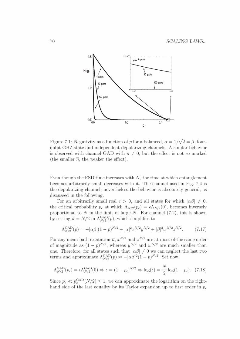
70 SCALING LAWS...
Figure 7.1: Negativity as a function of p for a balanced, α = 1/√
2 = β, four-qubit GHZ state and independent depolarizing channels. A similar behavioris observed with channel GAD with n 6= 0, but the effect is not so marked(the smaller n, the weaker the effect).
Even though the ESD time increases with N , the time at which entanglementbecomes arbitrarily small decreases with it. The channel used in Fig. 7.4 isthe depolarizing channel, nevertheless the behavior is absolutely general, asdiscussed in the following.
For an arbitrarily small real ǫ > 0, and all states for which |αβ| 6= 0,the critical probability pǫ at which ΛN/2(pǫ) = ǫΛN/2(0), becomes inverselyproportional to N in the limit of large N . For channel (7.2), this is shownby setting k = N/2 in ΛGAD
N/2 (p), which simplifies to
ΛGADN/2 (p) = −|αβ|(1 − p)N/2 + |α|2xN/2yN/2 + |β|2wN/2zN/2. (7.17)
For any mean bath excitation n, xN/2 and zN/2 are at most of the same orderof magnitude as (1 − p)N/2, whereas yN/2 and wN/2 are much smaller thanone. Therefore, for all states such that |αβ| 6= 0 we can neglect the last twoterms and approximate ΛGAD
N/2 (p) ≈ −|αβ|2(1 − p)N/2. Set now
ΛGADN/2 (pǫ) = ǫΛGAD
N/2 (0) ⇒ ǫ = (1 − pǫ)N/2 ⇒ log(ǫ) =
N
2log(1 − pǫ). (7.18)
Since pǫ ≪ pGADc (N/2) ≤ 1, we can approximate the logarithm on the right-
hand side of the last equality by its Taylor expansion up to first order in pǫ

7.5. CONCLUDING REMARKS 71
and write log(ǫ) = −N2pǫ, implying that
pGADǫ ≈ −(2/N) log(ǫ). (7.19)
Similar reasonings, applied to channels (7.3) and (7.4), lead to
pD,PDǫ (t) ≈ −(1/N) log(ǫ). (7.20)
Eqs. (7.19) and (7.20) assess the robustness of the state’s entanglement betterthan the ESD time. Much before ESD, negativity becomes arbitrarily small.The same behavior is observed for all studied channels, and all coefficients α,β 6= 0, despite the fact that for some cases, like for instance for channel (7.4),no ESD is observed. The presence of log ǫ in the above expression shows thatour result is quite insensitive to the actual value of ǫ≪ 1.
7.5 Concluding remarks
In this chapter I have probed the robustness of the entanglement of un-balanced GHZ states of arbitrary number of particles subject to independentenvironments. The states possess in general longer entanglement suddendeath time, the more particles in the system, but the time at which such en-tanglement becomes arbitrarily small is inversely proportional to the numberof constituent particles. The latter time characterizes better the robustness ofthe state’s entanglement than the time at which ESD itself occurs. In severalcases the action of the environment can naturally lead to bound entangledstates. An open question still remains on how other genuinely multipartiteentangled states, such as W-type or graph states, behave. Our results sug-gest that maintaining a significant amount of multiqubit entanglement inmacroscopic systems might be an even harder task than believed so far.

72 SCALING LAWS...
Figure 7.2: Negativity versus p for N = 4, 40 and 400, for the depolirizingchannel and for the most balanced partitions. In this graphic α = 1/3and β =
√8/3, but the same behavior is displayed for all other parameters
and maps. The inset shows a magnification of the region in which |ΛD2 (p)|
vanishes. Even though |ΛD40(p)| and |ΛD
400(p)| cross the latter and vanish muchlater, they become orders of magnitude smaller than their initial value longbefore reaching the crossing point.

Chapter 8
Identical particle entanglement
in Fermionic systems
Quantum correlations can naturally appear due to the indistinguishablecharacter of quantum systems. For example, the state of a pair of identicalfermions is always antisymmetric, hence naturally entangled. This entangle-ment comes from the indistinguishability of the fermions and can manifestitself in one or more degrees of freedom, depending, for example, on thespatial shape of the wave function [Ved03]. However, there is an interest-ing ongoing debate on the possibility of using this strictly spin-statisticalentanglement to perform quantum information tasks [ESBL04, GM04].
Usually, when talking about entanglement, one tends to ignore the role ofthe measurement apparatus, always considering ideal situations. However,there is no such a thing as an ideal detector, and the detector bandwidthaffects the measurement of entanglement. Furthermore, in the particularcase of identical particles, it is still not clear how the symmetry of detectionin external degrees of freedom affects the entanglement of the internal ones.
In this Chapter I will discuss the quantum correlations that naturallyarises in a non-interacting Fermi gas at zero temperature. In particular, Iwill analyze how the measurement of external degrees of freedom can affectthe entanglement in internal degrees of freedom in this system. Then, I willdiscuss how imperfect detections affect the observation of entanglement inthe fermionic gas.
A second step consists on proposing a scheme to extract entanglementcreated solely by the Pauli exclusion principle. In this scheme two indepen-dent photons excite non-interacting electrons in a semiconductor quantumwell. As the electrons relax to the bottom of the conduction band, thePauli exclusion principle forces quantum correlations between their spins. Itwill be shown that after the electron-hole recombination this correlation is
73

74 IDENTICAL PARTICLE ENTANGLEMENT
transferred to the emitted photons as entanglement in polarization, whichcan subsequently be used for quantum information tasks. This proposal isquite unorthodox in the sense that decoherence, usually viewed as an enemyof entanglement, actually plays an important role in the extraction of thisidentical particle entanglement.
The results contained in this chapter are due to collaborations with M.F. Santos, M. O. Terra Cunha, L. Malard, F. Matinaga, C. Lunkes, and V.Vedral.
8.1 Non-interacting Fermi gas
The symmetrization principle establishes that the quantum state of twoidentical particles must be symmetrized or anti-symmetrized according to theparticles species. However, in practice no physicist seems to care about theexistence of other particles that do not take part of the system under study.In his book, A. Peres analyzes this question and concludes that “ (...)it ishardly conceivable that observable properties of the particles in our labora-tory are affected by the possible existence on the Moon of another particleof the same species(...)”. However, until recently there was no formal studyconcerning this belief. In what follows I will describe some steps towards theunderstanding of correlations arising due to the Pauli principle.
8.1.1 Perfect detection
Suppose we pick up two fermion from a non-interacting Fermi gas atzero temperature, one at position r and the other at r′. What is the spinentanglement between them? Vedral showed that the amount of entangle-ment between these particles decreases with increasing distance betweenthem [Ved03]. He also showed that there is a limit below which any twofermions extracted from the gas are certainly entangled. In particular, ifboth fermions are extracted at the same position, then the Pauli exclusionprinciple forces their spin to be maximally entangled in a typical antisym-metric Bell state. In what follows I am going to briefly review these resultsand then present a clearer and more complete explanation to this behaviorthrough the analysis of the symmetry of the position detection.
The spin density matrix of these selected particles can be defined by
ρss′,tt′ = 〈Φ0|Ψ†t′(r
′)Ψ†t(r)Ψs′(r
′)Ψs(r) |Φ0〉 , (8.1)
where |φ0〉 is the ground state of the Fermi gas,
|φ0〉 = Πs,pb†s(p) |0〉 , (8.2)

8.1. NON-INTERACTING FERMI GAS 75
and the detection operator at position r and spin s is given by,
Ψ†s(r) =
∫ pf
0
d3p
(2π)3e−iprb†s(p). (8.3)
this integral is taken over the Fermi sphere with radio pf (the Fermi’s mo-mentum). The matrix elements (8.1) are second order correlation functions,which correspond to measuring these two fermions at positions r and r′.
The upper limit for guaranteed entanglement can be calculated applyingthe Peres-Horodecki criterion [Per96b] to the state (8.1). The following con-dition for the existence of entanglement holds: f 2 > 1
2, where f(r − r′) =
3j1(kF |r − r′|)/(kF |r − r′|), |r − r′| is the distance between the fermions,kF = pf/~ and j1 is a spherical Bessel function. This condition establishes aregion 0 ≤ |r − r′| < re, where re is the solution of f 2 = 1/2, for which thefermions are found to be entangled.
In order to get an interpretation of this result let me arrive at his resultin a different way. Define new detection operators:
Π+ss′(r, r
′) ≡ (Ψs(r)Ψs′(r′) + Ψs′(r)Ψs(r
′))√2
, (8.4a)
Π−ss′(r, r
′) ≡ (Ψs(r)Ψs′(r′) − Ψs′(r)Ψs(r
′))√2
. (8.4b)
The operator Π+ss′(Π
−ss′), detects the antisymmetric (symmetric) spatial part
and the symmetric (antisymmetric) spin part of fermion wavefunction.In terms of these new operators, Eq.(8.1) becomes:
ρss′,tt′ =1
2〈Φ0|[Π+†
tt′ (r, r′) + Π−†
tt′ (r, r′)][Π+
ss′(r, r′) + Π−
ss′(r, r′)]|Φ0〉 (8.5)
Note that written in this way, the two-fermion density matrix is the sum offour different terms, two of which contain only symmetric and antisymmetricspin detectors. The other two are the crossing terms, which vanish due tothe exclusion principle (spin and position of two fermions cannot be bothsymmetric or antisymmetric). The remaining terms are:
ρsym =1
2〈Φ0|Π+†
tt′ (r, r′)Π+
ss′(r, r′) |Φ0〉 , (8.6a)
ρasym =1
2〈Φ0|Π−†
tt′ (r, r′)Π−
ss′(r, r′) |Φ0〉 . (8.6b)
Here ρsym takes into consideration only the symmetric spin function (there-fore, it is related to the detection of the antisymmetric part of the spa-tial wavefunction) while ρasym contains only the antisymmetric spin function
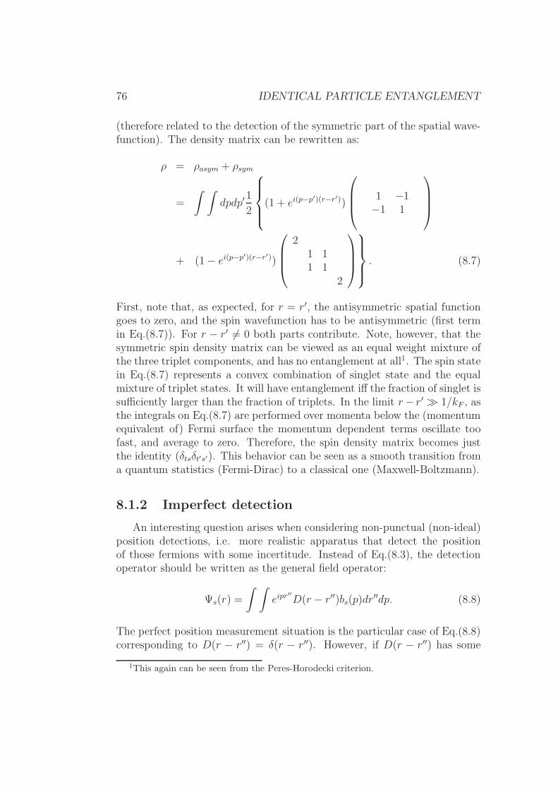
76 IDENTICAL PARTICLE ENTANGLEMENT
(therefore related to the detection of the symmetric part of the spatial wave-function). The density matrix can be rewritten as:
ρ = ρasym + ρsym
=
∫ ∫dpdp′
1
2
(1 + ei(p−p′)(r−r′))
1 −1−1 1
+ (1 − ei(p−p′)(r−r′))
21 11 1
2
. (8.7)
First, note that, as expected, for r = r′, the antisymmetric spatial functiongoes to zero, and the spin wavefunction has to be antisymmetric (first termin Eq.(8.7)). For r − r′ 6= 0 both parts contribute. Note, however, that thesymmetric spin density matrix can be viewed as an equal weight mixture ofthe three triplet components, and has no entanglement at all1. The spin statein Eq.(8.7) represents a convex combination of singlet state and the equalmixture of triplet states. It will have entanglement iff the fraction of singlet issufficiently larger than the fraction of triplets. In the limit r− r′ ≫ 1/kF , asthe integrals on Eq.(8.7) are performed over momenta below the (momentumequivalent of) Fermi surface the momentum dependent terms oscillate toofast, and average to zero. Therefore, the spin density matrix becomes justthe identity (δtsδt′s′). This behavior can be seen as a smooth transition froma quantum statistics (Fermi-Dirac) to a classical one (Maxwell-Boltzmann).
8.1.2 Imperfect detection
An interesting question arises when considering non-punctual (non-ideal)position detections, i.e. more realistic apparatus that detect the positionof those fermions with some incertitude. Instead of Eq.(8.3), the detectionoperator should be written as the general field operator:
Ψs(r) =
∫ ∫eipr
′′
D(r − r′′)bs(p)dr′′dp. (8.8)
The perfect position measurement situation is the particular case of Eq.(8.8)corresponding to D(r − r′′) = δ(r − r′′). However, if D(r − r′′) has some
1This again can be seen from the Peres-Horodecki criterion.

8.1. NON-INTERACTING FERMI GAS 77
position uncertainty, like, for example, if it is described by a gaussian withspread σ,
D(r − r′′) =1√2πσ
e−|r−r′′|2
2σ2 , (8.9)
then, the field operators become
Ψs(r) =1√2πσ
∫ ∫eipr
′′
e−|r−r′′|2
2σ2 bs(p)dr′′dp. (8.10)
These operators, when substituted back in Eq.(8.1), give:
ρss′,tt′ = δstδs′t′f(d, σ) + δst′δs′tg(d, σ), (8.11a)
with d = |r − r′|,
f(d, σ) =
(erf(σpf )
σ
)2
, (8.11b)
g(d, σ) =e
−d2
2σ2
σ2|erf(σpf −
id
2σ) − erf(− id
2σ)|2, (8.11c)
where erf(x) is the “error function”, defined via:
erf(x) ≡ 2√π
∫ x
0
e−t2
dt. (8.11d)
In order to make clearer the behavior of entanglement in relation tochanges in d and σ we can compute the negativity of the state ρ(d, σ, pf ):
N(ρ) = max{0,− f − 2g
4f − 2g} (8.12)
This function is plotted in Fig. 8.1 for some values of σ.Note that, for imperfect position detection, the entanglement decreases
as the detectors become apart from each other, but increases if the spreadin the detection becomes larger. The fact that inaccuracy in the detectionincreases entanglement may seem surprising at first sight. However it hasto be noted that as our knowledge in position gets worst, our knowledge inmomentum gets better. In the limit of infinite spread, both detectors becomeperfect momentum detectors (centered at p = 0, see Eq.(8.9)), which meansagain that their spin wavefunction should be totally antisymmetrized, hencethey are found in the antisymmetric Bell state. It is important to stress thatEq.(8.8) describes a coherent combination of localized field operators insteadof a statistical average of them. That is the reason for the infinite spreadlimit be a momentum-localized detector instead of just a vague “there is aparticle somewhere”.

78 IDENTICAL PARTICLE ENTANGLEMENT
Figure 8.1: N(ρ) vs. d for pf = 1 and σ = 1 (red), σ = 2 (green) and σ = 4(blue).
8.2 Useful entanglement from the Pauli prin-
ciple
In this section I would like to make the previous discussion less abstractand propose a way of observing this fermionic entanglement in a realisticsystem.
Consider that one excites a semi-conductor from its electronic groundstate by exactly promoting two electrons to the conduction band. These twoelectrons will be described by some quantum state with momentum and spindistribution. Due to phonon scattering, no matter the initial polarization,in a short time scale the spin state will be essentially random (supposingno energy difference between the possible polarizations). With the conditionthat relaxation time (τD) is much shorter than recombination time (τeh), theelectronic momentum distribution will tend to the bottom of the band. Infact, the quantum state will tend to the “ground state” of the band, whichcan be viewed as null momentum spin singlet, due to the Pauli principle.By the same time, but in a statistically independent way, electrons in thevalence band also relax, with the net effect of promoting the holes to the topof the band. Also supposing that the relaxation time of the holes is muchshorter than recombination time, there will be a singlet of holes in the top of

8.2. USEFUL ENTANGLEMENT FROM THE PAULI PRINCIPLE 79
the valence band. In this scheme, quantum correlations were created by thePauli principle through relaxation. The remaining question is whether thesecorrelations can be used to implement some quantum protocol.
Continuing with the argument, let me assume a selection rule for theradiative decay: electrons with spin +1/2 (−1/2) can only decay emittingphotons circularly polarized to the right (left) (Fig. ??B). After both elec-trons have decayed we will therefore obtain two photons in a polarizationentangled state, which can be used for different quantum information pro-tocols. I emphasize that this state is only obtained due to the existence offermionic entanglement between the electrons.
The idea described in the previous paragraphs can indeed be implementedin solid state physics. Two independent photons coming from single photonsources are used to create two electron-hole pairs of different k′s and spinsin a semiconductor quantum well. The system rapidly relax to the bottomof the conduction band. The electrons then emit photons recombining withthe holes in the valence band. For the argument presented before to hold,conduction and valence bands relaxation processes have to be much fasterthan the recombination time, which is the case in semiconductors (typicallyτD ∼ 10−12s and τeh ∼ 10−9s [Fat05]). Note that the emitted photons willbe entangled in polarization no matter in which direction they are emitted.However, in order to enhance the spontaneous recombination process and togive a preferred direction for the emission (also enhancing the probability ofdetection), the semiconductor can be placed inside an optical cavity [Yam91,WNIA92, BMYI91]. After escaping the cavity, these photons can be used forquantum information.
8.2.1 Selection rules
Take semiconductors of the group III-V [YC96] for which the conduction(valence) band has orbital angular momentum L = 0 (L = 1). The valenceband has two branches corresponding to heavy-holes (Jz = ±3/2) and light-holes (Jz = ±1/2) which are degenerate at k = 0 for bulk semiconductors.But in a semiconductor quantum well this degeneracy is lifted off due to theconfinement in one of the directions. Each new valence band still has theusual free-particle dispersion relation (E ∝ k2) around the energy gap, butthe gap itself is smaller for the heavy-hole electrons. Therefore, by shininglight of the proper frequency, it is possible to selectively excite electrons fromthe heavy-hole band without ever touching the light-hole ones (see Fig. 8.2).The electrons are excited by dipolar interaction, which means that there willbe a selection rule that couples each eigenstate in the heavy-hole band to apartner in the conduction band, depending only on the photon polarization

80 IDENTICAL PARTICLE ENTANGLEMENT
(see Fig. 8.3).
Figure 8.2: Band structure for the semiconductor quantum well -
For each value of k there can exist just two electrons according to the Pauliprinciple.
8.2.2 From fermions to photons
Let me now treat in some details what was described above. Supposewe have a semiconductor quantum well with exact two excitations with welldefined momentum k above the ground state (full valence band). Considerthe creation operator of two particles (electron + hole):
Ψ†s(k) = e†s(k)h
†s(−k), (8.13)
where e†s(k) (resp. h†s(k)) creates an electron (hole) in the conduction (va-lence) band with logical spin s and momentum k. The spin notation isutilized to emphasize correlation in the creation process, and the follow-ing correspondence between the real spins with the logical basis is impliedthrough the text:
|0〉 |1〉electrons -1/2 1/2
holes -3/2 3/2.
The spin state I am going to analize can be described by a spin densityoperator for the electrons and holes determined (up to normalization) by the
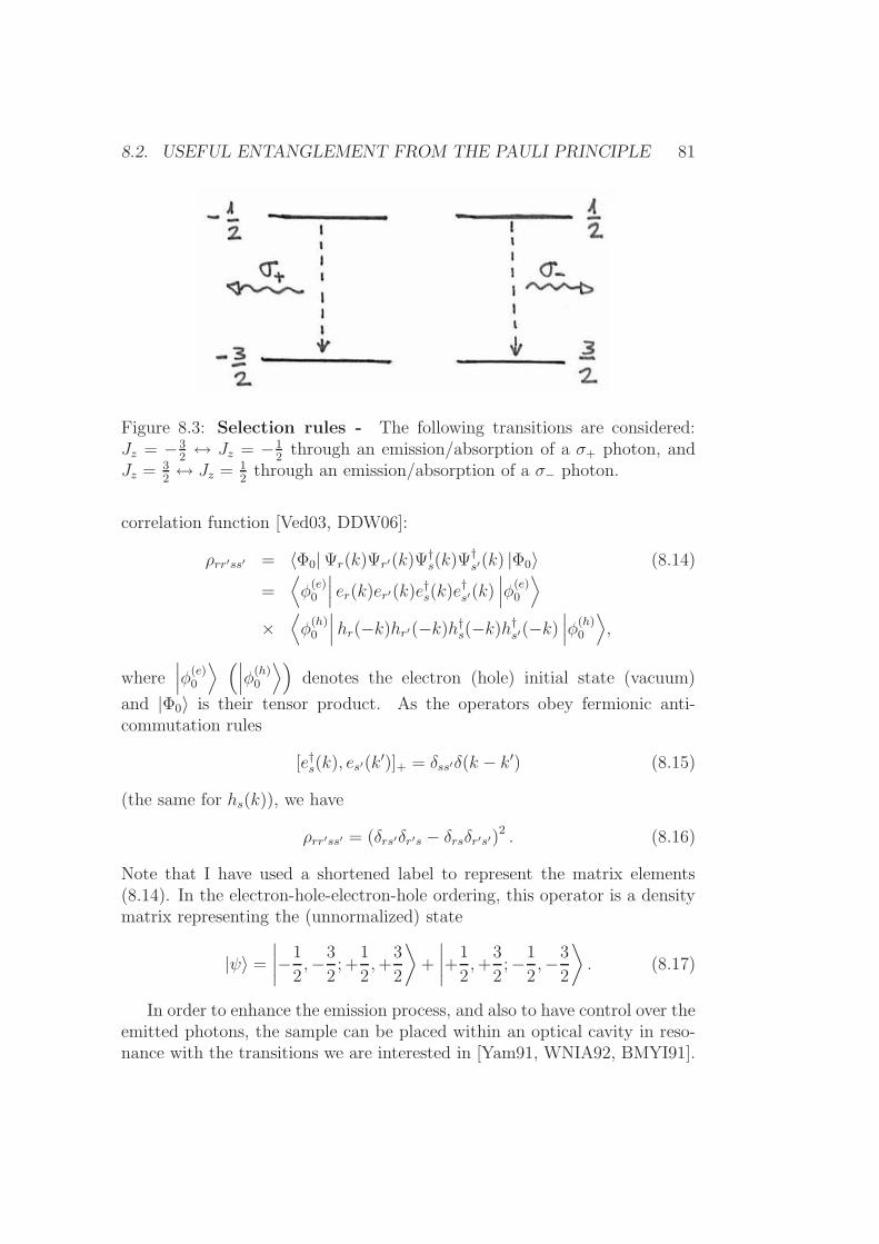
8.2. USEFUL ENTANGLEMENT FROM THE PAULI PRINCIPLE 81
Figure 8.3: Selection rules - The following transitions are considered:Jz = −3
2↔ Jz = −1
2through an emission/absorption of a σ+ photon, and
Jz = 32↔ Jz = 1
2through an emission/absorption of a σ− photon.
correlation function [Ved03, DDW06]:
ρrr′ss′ = 〈Φ0|Ψr(k)Ψr′(k)Ψ†s(k)Ψ
†s′(k) |Φ0〉 (8.14)
=⟨φ
(e)0
∣∣∣ er(k)er′(k)e†s(k)e†s′(k)∣∣∣φ(e)
0
⟩
×⟨φ
(h)0
∣∣∣hr(−k)hr′(−k)h†s(−k)h†s′(−k)∣∣∣φ(h)
0
⟩,
where∣∣∣φ(e)
0
⟩ (∣∣∣φ(h)0
⟩)denotes the electron (hole) initial state (vacuum)
and |Φ0〉 is their tensor product. As the operators obey fermionic anti-commutation rules
[e†s(k), es′(k′)]+ = δss′δ(k − k′) (8.15)
(the same for hs(k)), we have
ρrr′ss′ = (δrs′δr′s − δrsδr′s′)2 . (8.16)
Note that I have used a shortened label to represent the matrix elements(8.14). In the electron-hole-electron-hole ordering, this operator is a densitymatrix representing the (unnormalized) state
|ψ〉 =
∣∣∣∣−1
2,−3
2; +
1
2,+
3
2
⟩+
∣∣∣∣+1
2,+
3
2;−1
2,−3
2
⟩. (8.17)
In order to enhance the emission process, and also to have control over theemitted photons, the sample can be placed within an optical cavity in reso-nance with the transitions we are interested in [Yam91, WNIA92, BMYI91].

82 IDENTICAL PARTICLE ENTANGLEMENT
By the selection rules described above, the emitted photons state is
|σ−σ+〉 + |σ+σ−〉, (8.18)
which is a maximally entangled Bell state. Note that it is essential that theelectrons have the same momentum for the creation of a maximally entangledpair of photons.
We are interested in creating entangled photons from independent ones,and that is where decoherence plays an important role. Independent photonscreate electrons of different k′s. However, the incoherent energy losses to thenetwork phonons end up dragging those electrons to the conduction-bandground state (similarly the holes), where both of them have the same k = 0momentum! Taking into consideration the selectivity of the decay process,the photons will indeed be emitted in the Bell state of Eq. (8.18).
8.2.3 Some imperfections
The scenario that was discussed up to now is pretty much idealized. It isimportant to stress, however, that one very robust point in favor of this pro-posal is its independency on the specific model of decoherence used. When-ever the imposed conditions on the time scales are fulfilled, the state of thesystem before recombination will be very close to the one here described.And so the state of the emitted photons.
One posible way to mimic the effects of the imperfection in this approachis to consider a broadening in the momentum distribution, and also an im-perfect coincidence of the momenta. This can be taken into account bymodifying Eq. (8.13) to
Ψ†ss(k) =
∫∫f(kj − k)f(kj − k)e†s(kj)h
†s(kj)dkjdkj. (8.19)
This operator creates an electron with spin s and momentum distributiongiven by the function f(kj − k), and a hole with spin s and momentum
distribution given by f(kj − k). Later I will associate k = −k 2. With thisoperator, Eq. (8.14) can be rewritten as
2This association reflects the fact that an electron moving to a certain direction isequivalent to a hole moving to the opposite way.

8.2. USEFUL ENTANGLEMENT FROM THE PAULI PRINCIPLE 83
ρrr′ss′ =
∫f ∗(k0 − k)f ∗(k1 − k′)f(k2 − k)f(k3 − k′)
⟨φ
(e)0
∣∣∣ er(k0)er′(k1)e†s(k2)e
†s′(k3)
∣∣∣φ(e)0
⟩dk0...dk3
×∫f ∗(k0 − k)f ∗(k1 − k′)f(k2 − k)f(k3 − k′)
⟨φ
(h)0
∣∣∣hr(k0)hr′(k1)h†s(k2)h
†s′(k3)
∣∣∣φ(h)0
⟩dk0...dk3.
(8.20)
Anti-commutation rules (8.15) imply that the only non-null matrix ele-ments are:
ρ0000 = ρ1111 (8.21a)
= (L(k, k′) −M(k, k′))(L(k, k′) − M(k, k′)),
ρ0101 = ρ1010 = L(k, k′)L(k, k′), (8.21b)
ρ0110 = ρ1001 = M(k, k′)M(k, k′), (8.21c)
where
L(k, k′) =
∫dk0dk1|f(k0 − k)|2|f(k1 − k′)|2, (8.22a)
M(k, k′) =
∫dk0dk1f
∗(k0 − k)f ∗(k1 − k′)f(k1 − k)f(k0 − k′), (8.22b)
with similar expressions for L(k, k′) and M(k, k′) by changing k 7→ k and
k′ 7→ k′.The emitted photons (non-normalized) polarization state will thus be:
ρ =
(L−M)(L− M)
LL MM
MM LL
(L−M)(L − M)
, (8.23)
where I leave blank the null entries. Note that when k = k′ and k = k′
hold, L = M and L = M , giving a maximally entangled photonic state. No-tice the generality of this result: state (8.23) is written in terms of arbitrarymomentum distributions of the electrons before the decaying process. Forillustration, a chart of the entanglement between the two photons (charac-terized by the negativity) versus the difference in momentum distribution of
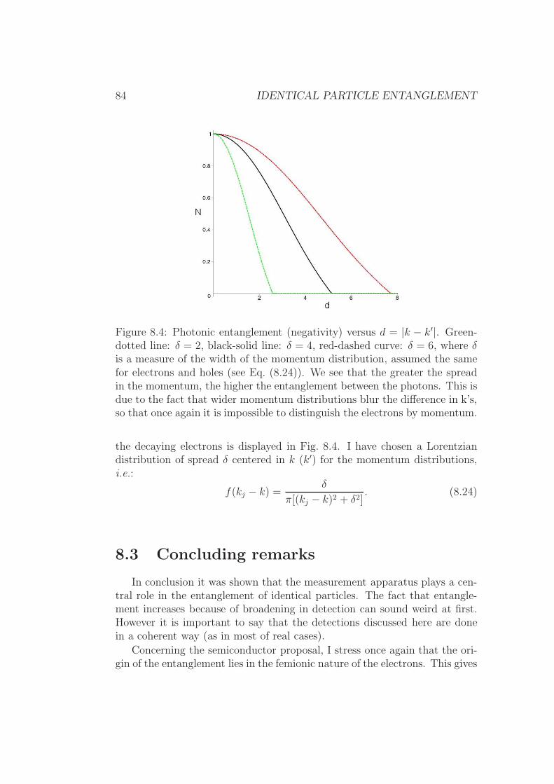
84 IDENTICAL PARTICLE ENTANGLEMENT
Figure 8.4: Photonic entanglement (negativity) versus d = |k − k′|. Green-dotted line: δ = 2, black-solid line: δ = 4, red-dashed curve: δ = 6, where δis a measure of the width of the momentum distribution, assumed the samefor electrons and holes (see Eq. (8.24)). We see that the greater the spreadin the momentum, the higher the entanglement between the photons. This isdue to the fact that wider momentum distributions blur the difference in k’s,so that once again it is impossible to distinguish the electrons by momentum.
the decaying electrons is displayed in Fig. 8.4. I have chosen a Lorentziandistribution of spread δ centered in k (k′) for the momentum distributions,i.e.:
f(kj − k) =δ
π[(kj − k)2 + δ2]. (8.24)
8.3 Concluding remarks
In conclusion it was shown that the measurement apparatus plays a cen-tral role in the entanglement of identical particles. The fact that entangle-ment increases because of broadening in detection can sound weird at first.However it is important to say that the detections discussed here are donein a coherent way (as in most of real cases).
Concerning the semiconductor proposal, I stress once again that the ori-gin of the entanglement lies in the femionic nature of the electrons. This gives
8.3. CONCLUDING REMARKS 85
a decisive positive answer to the question whether identical-particle entan-glement is useful for quantum information purposes. Specifically, identical-particle entanglement can in fact be extracted and converted to usual en-tanglement, and one important ingredient in this convertibility is the use ofmore than one degree of freedom.
Finally, I would like to emphasize the role played by the coupling to theenvironment in the discussed scheme. Usually, decoherence is seen as the roadfrom quantum to classical, implying information loss and entropy creation,which makes it a plague for quantum information tasks. However, a veryspecial situation occurs when decoherence is dictated by a null temperatureheat reservoir: after a transient time, the system asymptotically approachesits ground state. Whenever the ground state is nondegenerate, the result ofnull temperature decoherence is a pure state. When the system in question iscomposed, decoherence leads to statistical mixture, which tends to wash outentanglement. However, if, at zero temperature, the nondegenerate groundstate is also entangled, decoherence can actually create entangled states!That is a central part of the proposed scheme: here, decoherence plays thecrucial role of washing out the distinguishable origin of the input photons,allowing the extraction of entanglement from the Pauli principle.
Let me finish this chapter with a more practical issue. Ideally, the de-scribed setup could be viewed as a practical entangling machine, where theinput is a two photon unentangled state and the output an entangled state.Moreover, this machine would work on demand, i.e.: whenever we input twoindependent photons we receive back two entangled photons.


Chapter 9
Conclusions and Perspectives
Understanding entanglement is one of the biggest challenges physicistsare faced with. A lot of effort has been employed to get a complete theory ofthis resource, and also to apply it in real tasks. There are still many questionsinvolving entanglement, and some of them were not even cited in this thesis.The experimental production and use of entanglement in different systemsand scales, the computational hardness of classically simulating quantumeffects, and the link between entanglement and quantum phase transitionsare just few examples of these questions. All these points make entanglementcharacterization one of the most interdisciplinary branches of Physics.
In this thesis I have presented some results on the characterization ofentanglement I could address during the last years. Although the presentcontribution represents just few steps on entanglement theory, I hope theycan help to give a better understanding and to motivate future research onthis field. I would like to finish this text by raising some future research thatcould follow the presented ideas.
I have shown a connection between two entanglement quantifiers, the gen-eralized robustness of entanglement (Rg) and the geometric measure (EGME).This was made trough a lower bound to Rg based on EGME. It would beinteresting to find additional examples where this bound is tight and to seekfor the geometrical explanation of this fact. Furthermore whenever we havea way of calculating one of these measures, this gives a bound for the other.This might be useful because these quantities have also operational appeals[HMM+05, Bra07]. Seeking for relations among other entanglement quan-tifiers is also desirable as it can lead us to a better understanding on thedifferent forms of entanglement quantification.
Chapter 4 presented improvements on two big dilemmas concerning en-tanglement and non-locality. The first is the Peres’ conjecture that undistil-lable states never violate a Bell inequality. I have shown a partial proof of
87
88 CHAPTER 9. CONCLUSIONS AND PERSPECTIVES
this conjecture for the CFRD inequality by showing that all violating statesare NPT. A complementary result would be to prove that all violating statesare distillable. Further generalizations could consider other Bell inequalities,including those ones involving many measurement settings per site. On theother hand, finding a bound entangled state which violates a Bell inequalitywould disprove Peres’ conjecture1. The second big issue on this theme is tofind appropriate tests to prove non-locality, i.e.: loop-hole free experiments.Quadratures of the electromagnetic field is a promising degree of freedomwhere this tests could be proposed. First, photons can be distributed overlong distances using optical fibers or even in free-space. Second, quadraturemeasurements attain incredibly high efficiencies through homodyning.
Concerning the study of the geometry of entanglement I hope the pre-sented method for investigating the boundary features of separable sets cangive us a better idea on the mathematical description of quantum states.It is interesting that singularities in these sets appear in physical phenom-ena. An open question consists in looking for physical consequences of thesesingularities (if any).
Many are the open questions on the entanglement properties of decoheredstates. First, a whole line of research consists in the study of the quantum-classical transition, and entanglement certainly plays a major role in thisarena. Furthermore, as said before, it is crucial to understand the degra-dation of entanglement in real protocols since it is a valuable resource. Inthis sense further studies should include other multipartite states (e.g.: W,cluster, and CV states) and other decoherence models. In the end the bigquery is whether scalable quantum computation is possible.
Finally, the entanglement properties of many body systems is among thehottest lines of research nowadays. The Fermi gas is a first approximationfor many systems and it is then important to understand the features of thismodel. Moreover, we could propose a realistic system where the discussedeffects could be seen. In my opinion, an implementation of this scheme, iffeasible, would be interesting not only from a fundamental but also from apractical point of view.
1Here I mean bound entangled among all the partitions.

Appendix A
Multipartite entanglement
In this chapter I will discuss in more details the different kinds of multi-partite entanglement.
When several parts are involved we can have different notions of entan-glement, depending on the partition we apply to this state [DC00, DCT99,ABLS01, EG06]. For example, in a tripartite scenario, some states can bewritten as
ρABC = ρAB ⊗ ρC , (A.1)
where ρAB is an entangled state. This state is separable according to thepartition AB|C and can be built by joint operations on particles A and Band independent single operations on C. Hence it is said that such a ρABC
has no tripartite entanglement.We could go further in the classification of entanglement and define convex
combinations of states like (A.1),i.e.:
ρ =∑
i
piρABi ⊗ ρCi + qiρ
Ai ⊗ ρBCi + riρ
ACi ⊗ ρBi , (A.2)
with pi, qi, ri ≥ 0 and∑
i pi + qi + ri = 1. To build these states we again donot need to perform joint operations on the three particles, but instead canuse just (classically) correlated two-particle operations. Because of that fact,states (A.2) do not have genuine tripartite entanglement. However somethem do have entanglement among the three particles, since they cannot bewritten as (A.1) for example. This classification can be extended for statescomposed by more than three parties straightforwardly.
Note that each one of these sets is convex. Fully separable states form asubset of the set of biseparable states like (A.1), which by the other hand isa subset of the set of states like (A.2), and so on. We thus have a hierarchyof entangled states, and we can see the set of quantum states as composedhaving an onion-like structure (see Fig.A.1).
89

90 APPENDIX A. MULTIPARTITE ENTANGLEMENT
Figure A.1: State space structure.
As commented in Chapter 1, when talking about multipartite entangle-ment we can define different kinds of separability. Suppose a state ρ canbe written as a convex combination of states which are product of k tensorfactors. The state ρ is then said to be a k-separable state. One should notethat in a system of n parts, n-separability means that none of the subsystemsshare quantum correlations with the others. Besides, every state is trivially1-separable. The set of k-separable states will be denoted by Sk. It is clearthat Sn ⊂ Sn−1 ⊂ ... ⊂ S1 = D, where D denotes the set of density operators.

Appendix B
RkR as a detector of singularities
in Sk
In this Appendix we aim to prove Proposition 1, in Chapter 6. This canbe done in a more general way through the following result:
Proposition 2 Let D be a closed, convex set. Let S ⊂ D also be closedand convex, with π a point in the interior of S. If ∂S is a Cm manifold andthe states ρ(q) describe a Cm curve in D with no points in the interior of Sand obeying the condition that the tangent vector ρ′ (q) is never parallel toπ − ρ (q), then RR(ρ(q)) is also a Cm function.
One must remember that a manifold is called Cm if it can be parameterizedby functions with continuous derivatives up to order m [?]. The reader canchange Cm by smooth, in the usual sense of C∞, with almost no loss (actually,we use smooth throughout this Letter in the less precise sense of “as regularas necessary”). Other topological remarks before the proof: the fact that Shas interior points implies that S and D have the same dimensionality (sincethere is an open ball of D contained in S), and the proof will use the notionof (topological) cone, which simply means the union of all segments from agiven point V to each point of a given set A: this is called the cone of A withvertex V .Proof: The geometrical situation leads to the cone, given by (p, q) 7→ p π+(1 − p) ρ (q), p ∈ [0, 1]. The condition on the tangent vector (together withthe fact that π is interior to S, while ρ (q) has no point in this interior) issufficient for this cone to be Cm, except at the vertex π, at least locally in q.
As S is bounded and convex, and π is in its interior, every straight linefrom π crosses ∂S exactly once. As ρ (q) has no point in the interior of S,this crossing always happens for 0 ≤ p < 1. Denote this crossing value by
91

92 RkR as a detector...
pc (q). The curve q 7→ pc (q) π + (1 − pc (q)) ρ (q) is Cm, implying pc is a Cm
function of q.The random robustness is given by RR (ρ (q)) = pc
1−pc. As pc < 1, we also
obtain that RR is a Cm function of q. �

Appendix C
Experimental Setup
In this appendix it will be shown the details of the setup used in theexperiment described in Chapter 6.
Figure C.1: Experimental setup.
The state source is composed by a 2mm-thick BBO (β-BaB2O4) nonlinearcrystal (C1) pumped by a cw krypton laser operating at 413nm, generatingphoton pairs at 826nm by type II spontaneous parametric down-conversion.Crystal C1 is cut and oriented to generate either one of the polarizationentangled Bell states |Ψ−〉 or |Ψ+〉. Walk-off and phase compensation isprovided by the half-wave plate H0 followed by a 1mm-thick BBO crystal(C2) [KMW+05], together with two 1mm-thick crystalline quartz plates (Z)
93

94 APPENDIX C. EXPERIMENTAL SETUP
inserted in one of the down-converted photon paths. The unconverted laserbeam transmitted by crystal C1 is discarded by means of a dichroic mirror(U). The detection stages are composed by photon counting diode modulesD1 and D2, preceded by 8nm FWHM interference filters F1 and F2 centeredat 825nm, and by circular apertures A1 of 1.6mm∅ and A2 of 3.0mm ∅. Singleand coincidence counts with 5ns resolving time are registered by a computercontrolled electronic module (CC). Polarization analyzers are composed byquarter-wave plates Q1 and Q2, half-wave plates H1 and H2, followed bypolarizing cubes P1 and P2. The State Source produces state |Ψ−〉. Foreach pair, the photon emerging in the upper path goes straight to the po-larization analyzer and to the detection stage 1. The lower path photon isdirected by mirror M3 through the circular aperture A3 into the state mixer(an unbalanced Michelson interferometer), composed by the beam splitterBS, mirrors M4 and M5, quarter-wave plates Q4 and Q5, variable circularapertures A4 and A5, and by the half-wave plate H3, whose purpose is tocompensate for an unwanted slight polarization rotation caused by the beamsplitter. The quarter-wave plate Q4 is switched off which means that if thelower photon follows path labeled 4, there is no change to its polarizationand the half-wave plate H3 changes the state to |Ψ+〉. On the other hand,if the lower photon follows path labeled 5, Q5 is oriented with the fast axisat 45◦ in order to flip its polarization. The path length difference, 130mm,is much larger than the coherence length of the down-converted fields, en-suring an incoherent recombination at BS. The pair detected by CC is instate q|Ψ+〉〈Ψ+|+ (1− q)|Φ+〉〈Φ+| where q is defined by the relative sizes ofapertures A4 and A5.
Appendix D
Full separability of GHZ states
under the Amplitude Damping
Channel
Here we prove that the amplitude damping channel leads the state (7.1)to a fully separable state when all of its bipartite entanglements vanish.
Proof: First of all note that the evolved density matrix can be writtenas ρ = |α|2(|0〉 〈0| |)⊗N + ρs, where ρs is an unnormalized state. The goalis to show that ρs is fully separable. This will be done by defining a fullyseparable state σ and showing a local measurement protocol, a local POVM[?], which transforms σ into ρs with certain probability. Because only localoperations are applied we will conclude that ρs, and then ρ, must be fullyseparable.
The (unnormalized) state σ is defined as σ = β2(1−p)N{I+(|0〉 〈1| |)⊗N+(|1〉 〈0| |)⊗N}, being I the 2N × 2N identity matrix. State σ is GHZ-diagonal(see def. in Ref. [DC00]) and all of its negativities are null. Hence, by theDur-Cirac-Tarrach criterion [DCT99], σ is fully separable. Consider, for each
qubit i, the local POVM {A(i)m }2
m=1 with elements A(i)1 = δ(
√p
1−p |0〉 〈0| | +|1〉 〈1| |), where δ is such that A
(i)†
1 A(i)1 ≤ I, and A
(i)†
2 A(i)2 = I−A(i)†
1 A(i)1 . One
can see that by applying this POVM for every qubit of state σ, when themeasurement outcome is m = 1 (corresponding to A1) for all the qubits, thefinal state is nothing but ρs.�
95


Appendix E
Resumen
La mecanica cuantica fue concebida como una teorıa capaz de describirlos fenomenos fısicos a nivel atomico. Rapidamente fue aplicada en otroscasos como el estudio de la dispersion de las partıculas y de la interaccionentre la luz y la materia.
La primera crıtica importante a la teorıa cuantica fue hecha por Einstein,Podolski y Rosen (EPR) en su artıculo titulado ”Can quantum-mechanicaldescription of physical reality be considered complete?” [EPR35]. Estos au-tores resaltan que a pesar de que la teorıa cuantica acierta al describir cor-rectamente muchos fenomenos fısicos, tambien permite hacer prediccionesextranas como la accion instantanea entre objetos distantes. En el fondo, elargumento expuesto por EPR estaba basado en la posibilidad de tener unestado entrelazado. Basandose en las criticas de EPR, Schodinger llamo laatencion sobre el hecho de que alguno estados cuanticos pueden ser mejorentendidos cuando son investigados como un todo y no a traves de cada unode sus subsistemas [Sch35].
Muchos anos despues J. Bell puso esta discusion en un ambito mas firme.Aceptando la idea de realismo local introducida por EPR, Bell desarrollosus famosas desigualdades incluyendo estadısticas de medidas hechas en sis-temas compuestos [Bel87]. A partir de entonces la discusion acerca de lano-localidad de la mecanica cuantica podıa ser hecha a un nivel experimen-tal. Unos anos despues los primeros resultados experimentales usando lasdesigualdades de Bell fueran reportados [FC72, FT76, AGG81, ADG82] ydieron fuerza a la creencia de la no-localidad de la mecanica cuantica. Dadoestados que no son entrelazados nunca podrıan violar una desigualdad deBell, estas pruebas pueden ser vistas como las primeras observaciones exper-imentales de entrelazamiento.
Hasta los anos 90, la discusion acerca del entrelazamiento se hizo a unnivel mas fundamental, el de los pilares mismos de la teorıa cuantica. Fue
97
98 APPENDIX E. RESUMEN
despues de las primeras propuestas de protocolos de informacion cuantica,que el termino ”entrelazamiento” paso a tener una connotacion de ”recurso”,capaz de proporcionar ventajas sobre las maneras clasicas de procesar infor-macion [NC00, BEZ00]. En 1991, un protocolo de criptografıa totalmentebasado en el entrelazamiento fue propuesto [Eke91]. Para entonces ya sesabıa que el entrelazamiento no era algo necesario para garantizar la seguri-dad de la comunicacion [BB84, BBD92]. Quizas fue el descubrimiento de lateleportacion cuantica el cambio mas grande en la teorıa del entrelazamiento[BBC+93]. Desde entonces quedo clara la importancia de este recurso paraaplicaciones practicas.
A partir de ese momento la teorıa del entrelazamiento empezo su propiocamino y gano el status de disciplina independiente. Entre los objetivos prin-cipales de la teorıa del entrelazamiento estan el desarrollo de un formalismomatematico que pueda describir este recurso, la busqueda de sus aplicaciones,la investigacion de la conexion del entrelazamiento con otros fenomenos fısicosy, volviendo a aspectos mas fundamentales, la importancia del entrelaza-miento para los fundamentos de la mecanica cuantica. Actualmente la liter-atura acerca del entrelazamiento es enorme. El objetivo de esa tesis no es pro-porcionar una revision en este tema, pero contribuir con resultados originales.Revisiones acerca del entrelazamiento pueden ser encontradas en las referen-cias [HHHH07, AFOV07, PV05, Bru02, Ter02, PV98, Ver02, Eis01, EP03].Las cuestiones abiertas acerca del entrelazamiento van desde su descripcionmatematica hasta su utilizacion. Entre todos esos aspectos, en esta tesis yoaborde aquellos que mas me motivaron durante mi doctorado.
A pesar de que la definicion matematica del entrelazamiento es sencilla,el problema de determinar si un estado cuantico general esta entrelazado ono es muy difıcil [Ter02, HHHH07]. Una de las ramas mas importantes dela teorıa del entrelazamiento se centra en encontrar tecnicas que sean ca-paces de resolver este problema. El paso siguiente, despues de determinar siun estado esta entrelazado, serıa determinar la cantidad de entrelazamientopresente en el sistema [PV98]. Para esto se usan los cuantificadores de entre-lazamiento, un conjunto de reglas que se puede aplicar a un estado cuanticopara decidir su contenido de entrelazamiento. Una de las primeras manerasde cuantificar el entrelazamiento fue determinar la capacidad de cada es-tado en realizar tareas de informacion cuantica [BBP+96, BDSW96]. Estaforma de abordar el problema, a pesar de ser muy productiva depende pro-fundamente de cada tarea en cuestion. Una manera mas abstracta de tratareste problema consiste en determinar un conjunto de reglas que un cuan-tificador de entrelazamiento debe seguir, sin preocuparse por su significadofısico [Vid00, VPRK97]. Finalmente, podemos tambien utilizar conceptosgeometricos para cuantificar el entrelazamiento. Podemos organizar los esta-
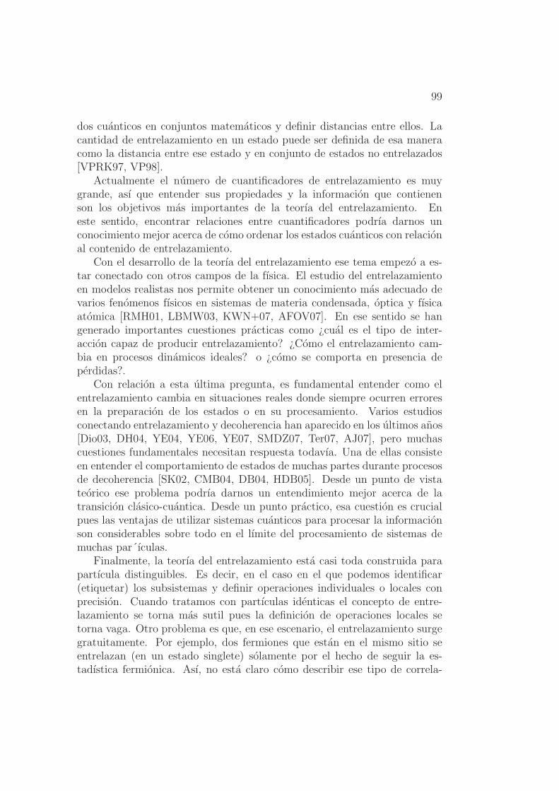
99
dos cuanticos en conjuntos matematicos y definir distancias entre ellos. Lacantidad de entrelazamiento en un estado puede ser definida de esa maneracomo la distancia entre ese estado y en conjunto de estados no entrelazados[VPRK97, VP98].
Actualmente el numero de cuantificadores de entrelazamiento es muygrande, ası que entender sus propiedades y la informacion que contienenson los objetivos mas importantes de la teorıa del entrelazamiento. Eneste sentido, encontrar relaciones entre cuantificadores podrıa darnos unconocimiento mejor acerca de como ordenar los estados cuanticos con relacional contenido de entrelazamiento.
Con el desarrollo de la teorıa del entrelazamiento ese tema empezo a es-tar conectado con otros campos de la fısica. El estudio del entrelazamientoen modelos realistas nos permite obtener un conocimiento mas adecuado devarios fenomenos fısicos en sistemas de materia condensada, optica y fısicaatomica [RMH01, LBMW03, KWN+07, AFOV07]. En ese sentido se hangenerado importantes cuestiones practicas como ¿cual es el tipo de inter-accion capaz de producir entrelazamiento? ¿Como el entrelazamiento cam-bia en procesos dinamicos ideales? o ¿como se comporta en presencia deperdidas?.
Con relacion a esta ultima pregunta, es fundamental entender como elentrelazamiento cambia en situaciones reales donde siempre ocurren erroresen la preparacion de los estados o en su procesamiento. Varios estudiosconectando entrelazamiento y decoherencia han aparecido en los ultimos anos[Dio03, DH04, YE04, YE06, YE07, SMDZ07, Ter07, AJ07], pero muchascuestiones fundamentales necesitan respuesta todavıa. Una de ellas consisteen entender el comportamiento de estados de muchas partes durante procesosde decoherencia [SK02, CMB04, DB04, HDB05]. Desde un punto de vistateorico ese problema podrıa darnos un entendimiento mejor acerca de latransicion clasico-cuantica. Desde un punto practico, esa cuestion es crucialpues las ventajas de utilizar sistemas cuanticos para procesar la informacionson considerables sobre todo en el lımite del procesamiento de sistemas demuchas par´ıculas.
Finalmente, la teorıa del entrelazamiento esta casi toda construida parapartıcula distinguibles. Es decir, en el caso en el que podemos identificar(etiquetar) los subsistemas y definir operaciones individuales o locales conprecision. Cuando tratamos con partıculas identicas el concepto de entre-lazamiento se torna mas sutil pues la definicion de operaciones locales setorna vaga. Otro problema es que, en ese escenario, el entrelazamiento surgegratuitamente. Por ejemplo, dos fermiones que estan en el mismo sitio seentrelazan (en un estado singlete) solamente por el hecho de seguir la es-tadıstica fermionica. Ası, no esta claro como describir ese tipo de correla-
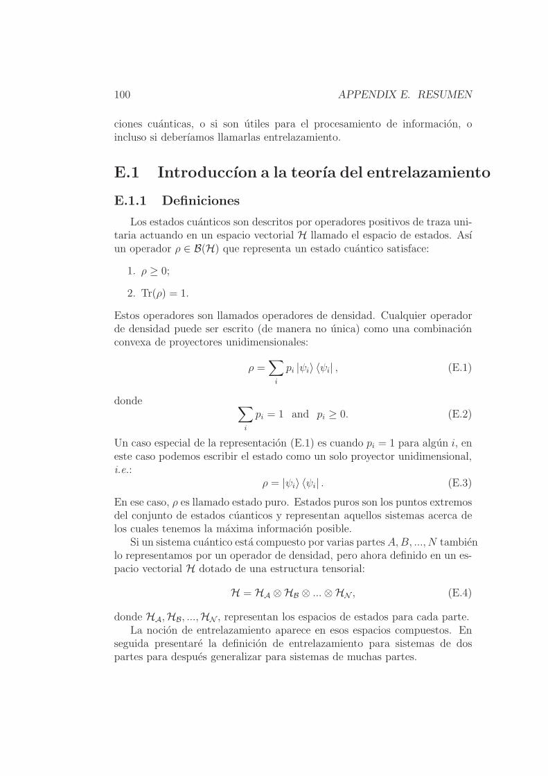
100 APPENDIX E. RESUMEN
ciones cuanticas, o si son utiles para el procesamiento de informacion, oincluso si deberıamos llamarlas entrelazamiento.
E.1 Introduccıon a la teorıa del entrelazamiento
E.1.1 Definiciones
Los estados cuanticos son descritos por operadores positivos de traza uni-taria actuando en un espacio vectorial H llamado el espacio de estados. Asıun operador ρ ∈ B(H) que representa un estado cuantico satisface:
1. ρ ≥ 0;
2. Tr(ρ) = 1.
Estos operadores son llamados operadores de densidad. Cualquier operadorde densidad puede ser escrito (de manera no unica) como una combinacionconvexa de proyectores unidimensionales:
ρ =∑
i
pi |ψi〉 〈ψi| , (E.1)
donde ∑
i
pi = 1 and pi ≥ 0. (E.2)
Un caso especial de la representacion (E.1) es cuando pi = 1 para algun i, eneste caso podemos escribir el estado como un solo proyector unidimensional,i.e.:
ρ = |ψi〉 〈ψi| . (E.3)
En ese caso, ρ es llamado estado puro. Estados puros son los puntos extremosdel conjunto de estados cuanticos y representan aquellos sistemas acerca delos cuales tenemos la maxima informacion posible.
Si un sistema cuantico esta compuesto por varias partes A,B, ..., N tambienlo representamos por un operador de densidad, pero ahora definido en un es-pacio vectorial H dotado de una estructura tensorial:
H = HA ⊗HB ⊗ ...⊗HN , (E.4)
donde HA,HB, ...,HN , representan los espacios de estados para cada parte.La nocion de entrelazamiento aparece en esos espacios compuestos. En
seguida presentare la definicion de entrelazamiento para sistemas de dospartes para despues generalizar para sistemas de muchas partes.

E.1. INTRODUCCION A LA TEORIA DEL ENTRELAZAMIENTO 101
Definicion - Separabilidad de estados bipartidos: Estados bipar-tidos entrelazados son aquellos que no pueden ser escritos como una com-binacion convexa de productos de operadores de densidad. Dicho de otraforma, ρ ∈ B(HA ⊗HB) es entrelazado si y solo si
ρ 6=∑
i
piρAi ⊗ ρBi , (E.5)
donde {pi} es una distribucion de probabilidades. Los estados que puedenser escritos como (E.5) son llamados estados separables.
Un ejemplo de un estado entrelazado es |Φ+〉 = (|00〉 + |11〉) /√
2.En el caso de sistemas de dos partes tenemos solo que diferenciar estados
entrelazados de estados separables. Cuando hay muchas partes, un estadopuede tener entrelazamiento solamente entre algunas de las partes. Un ejem-plo es el estado
(|00〉 + |11〉)√2
⊗ (|00〉 + |11〉)√2
. (E.6)
Este tipo de estados posee entrelazamiento entre las dos primeras partıculasy tambien entre las dos ultimas, mientras que no hay entrelazamiento entreesos dos bloques de partıculas. En ese contexto surgen maneras distintasde entrelazar un sistema. Tenemos entonces que definir la k-separabilidad[DCT99, DC00, ABLS01]:
Definition 3 - k-separabilidad: Un estado cuantico es llamado k-separablesi puede ser escrito como una combinacion convexa de estados que son unproducto de como maximo k factores.
E.1.2 Detectando el entrelazamiento
Dado un estado general ρ, ¿como podemos determinar si esta entrelazado?Inicialmente podrıamos intentar escribir ρ como en (E.5). Pero, como ρadmite infinitas representaciones por combinaciones convexas, la tarea debuscar, entre todas las representaciones, si alguna es equivalente a (E.5) setorna impracticable. Claramente tenemos que desarrollar metodos mas efi-caces para detectar el entrelazamiento. Siguiendo esa idea varios criteriosde entrelazamientos fueron propuestos en los ultimos anos [Ter02]. Desgraci-adamente no hay una prueba definitiva para comprobar la separabilidad deestados generales.
Entre los criterios de entrelazamiento mas utilizados estan:
• Desigualdades de Bell [Bel87, Ter00, WW01b, Gis07].
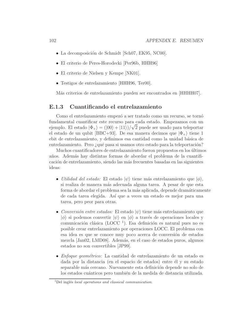
102 APPENDIX E. RESUMEN
• La decomposicion de Schmidt [Sch07, EK95, NC00].
• El criterio de Peres-Horodecki [Per96b, HHH96]
• El criterio de Nielsen y Kempe [NK01].
• Testigos de entrelazamiento [HHH96, Ter00].
Mas criterios de entrelazamiento pueden ser encontrados en [HHHH07].
E.1.3 Cuantificando el entrelazamiento
Como el entrelazamiento empezo a ser tratado como un recurso, se tornofundamental cuantificar este recurso para cada estado. Empezamos con unejemplo. El estado |Φ+〉 = (|00〉+ |11〉)/
√2 puede ser usado para teleportar
el estado de un qubit [BBC+93]. De esa manera decimos que |Φ+〉 tiene 1ebit de entrelazamiento, y definimos esa cantidad como la unidad basica deentrelazamiento. Pero ¿que pasa si usamos otro estado para la teleportacion?
Muchos cuantificadores de entrelazamiento fueron propuestos en los ultimosanos. Ademas hay distintas formas de abordar el problema de la cuantifi-cacion de entrelazamiento, siendo las mas frecuentes basadas en las siguientesideas:
• Utilidad del estado: El estado |ψ〉 tiene mas entrelazamiento que |φ〉,si realiza de manera mas adecuada alguna tarea. A pesar de que estaforma de abordar el problema sea la mas aplicada, depende dramaticamentede cada tarea elegida. Ası que a veces un estado es mejor para unatarea, pero peor para otras.
• Conversion entre estados: El estado |ψ〉 tiene mas entrelazamiento que|φ〉 si podemos convertir |ψ〉 en |φ〉 a traves de operaciones locales ycomunicacion clasica (LOCC 1). Esa definicion es natural pues no esposible crear entrelazamiento por operaciones LOCC. El problema conesa idea es que se conoce muy poco acerca de conversion de estadosmezcla [Jan02, LMD08]. Ademas, en el caso de estados puros, algunosestados no son convertibles [JP99].
• Enfoque geometrico: La cantidad de entrelazamiento de un estado esdada por la distancia (en el espacio de estados) entre el y su estadoseparable mas cercano. Nuevamente esta definicion depende no solo delos estados cuanticos pero tambien de la medida de distancia utilizada.
1Del ingles local operations and classical communication.
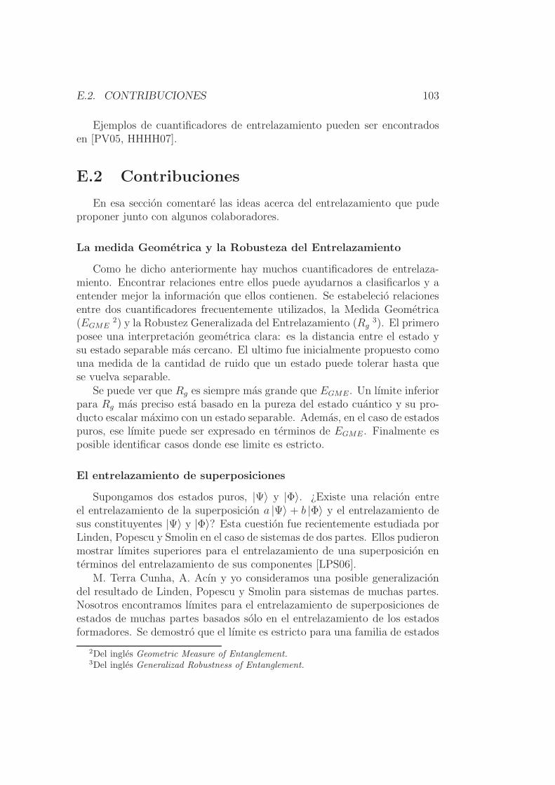
E.2. CONTRIBUCIONES 103
Ejemplos de cuantificadores de entrelazamiento pueden ser encontradosen [PV05, HHHH07].
E.2 Contribuciones
En esa seccion comentare las ideas acerca del entrelazamiento que pudeproponer junto con algunos colaboradores.
La medida Geometrica y la Robusteza del Entrelazamiento
Como he dicho anteriormente hay muchos cuantificadores de entrelaza-miento. Encontrar relaciones entre ellos puede ayudarnos a clasificarlos y aentender mejor la informacion que ellos contienen. Se estabelecio relacionesentre dos cuantificadores frecuentemente utilizados, la Medida Geometrica(EGME
2) y la Robustez Generalizada del Entrelazamiento (Rg3). El primero
posee una interpretacion geometrica clara: es la distancia entre el estado ysu estado separable mas cercano. El ultimo fue inicialmente propuesto comouna medida de la cantidad de ruido que un estado puede tolerar hasta quese vuelva separable.
Se puede ver que Rg es siempre mas grande que EGME . Un lımite inferiorpara Rg mas preciso esta basado en la pureza del estado cuantico y su pro-ducto escalar maximo con un estado separable. Ademas, en el caso de estadospuros, ese lımite puede ser expresado en terminos de EGME . Finalmente esposible identificar casos donde ese limite es estricto.
El entrelazamiento de superposiciones
Supongamos dos estados puros, |Ψ〉 y |Φ〉. ¿Existe una relacion entreel entrelazamiento de la superposicion a |Ψ〉 + b |Φ〉 y el entrelazamiento desus constituyentes |Ψ〉 y |Φ〉? Esta cuestion fue recientemente estudiada porLinden, Popescu y Smolin en el caso de sistemas de dos partes. Ellos pudieronmostrar lımites superiores para el entrelazamiento de una superposicion enterminos del entrelazamiento de sus componentes [LPS06].
M. Terra Cunha, A. Acın y yo consideramos una posible generalizaciondel resultado de Linden, Popescu y Smolin para sistemas de muchas partes.Nosotros encontramos lımites para el entrelazamiento de superposiciones deestados de muchas partes basados solo en el entrelazamiento de los estadosformadores. Se demostro que el lımite es estricto para una familia de estados
2Del ingles Geometric Measure of Entanglement.3Del ingles Generalizad Robustness of Entanglement.

104 APPENDIX E. RESUMEN
compuestos por un numero arbitrario de qubits. Ademas nuestros resultadostambien se extienden a un conjunto amplio de cuantificadores de entrelaza-miento, incluyendo la negatividad, la robustez del entrelazamiento y la medidade la mejor aproximacion separable.
Entrelazamiento PPT y violacion de desigualdades de Bell para
variables continuas
Inspirado por las similitudes entre los procesos de destilacion del entre-lazamiento [BDSW96] y la deteccion de la no-localidad escondida [Pop95,Per96a], A. Peres conjeturo que todos los estados no distilables admiten unadescripcion a traves de modelos realistas locales. O sea, esos estados no vi-olan desigualdades de Bell. Esa conjetura fue demostrada apenas en el casodonde dos medidas individuales binarias son aplicadas a un sistema de Npartes.
Recientemente una nueva desigualdad de Bell para variables continuasutilizando operadores no-acotados fue propuesta [CFRD07]. Utilizando esadesigualdad A. Salles, A. Acın y yo pudimos extender la conjetura de Perespara el caso continuo y probar que todos los estados con una transposicionparcial positiva satisfacen la desigualdad.
Clarificando la geometrıa del entrelazamiento
El conjunto de los estados cuanticos es cerrado y convexo: combinacionesconvexas de estados cuanticos son estados cuanticos. El conjunto de los esta-dos separables es un subconjunto, que tambien es cerrado y convexo. Ademasde esas caracterısticas que son consecuencias directas de la definicion de es-tados cuanticos y estados separables, otras preguntas surgen de ese analisis.¿Como es la forma de esos conjuntos? ¿Cual es su volumen? ¿Como carac-terizar esas cantidades? ¿Estan estas cantidades directamente relacionadascon fenomenos fısicos?
En una colaboracion con M. Terra Cunha, M. F. Santos, F. Brandao,P. Lima, O. Cosme, S. Padua, y C. Monken, propusimos un metodo parainvestigar la forma del conjunto de estados separables. Para ello utilizamosun cuantificador de entrelazamiento llamado robustez aleatoria del entrelaza-miento. Ese cuantificador puede ser usado como un microscopio para investi-gar la frontera del conjunto de estados separables. Ademas, como esta inves-tigacion puede ser hecha a un nivel experimental, llevamos a cabo un exper-imento con fotones entrelazados para ilustrar nuestras predicciones teoricas.Singularidades en el conjunto de estados separables para dos qubits fueronencontradas. Esas singularidades aparecen naturalmente en fenomenos como
E.2. CONTRIBUCIONES 105
la transferencia de entrelazamiento en sistemas de spines sujetos a camposmagneticos variables y en procesos de decoherencia.
Entrelazamiento de muchas partıculas y decoherencia
En el mundo real no es posible generar un estado cuantico puro. Debidoa errores en la preparacion de los estados y ruido en su dinamica siempretratamos con estados mezcla. El entrelazamiento es muy sensible a esosprocesos ruidosos y esa es seguramente la principal dificultad para la imple-mentacion real de protocolos de informacion cuantica. Ademas el fenomenode decoherencia esta en la esencia de la transicion entre el mundo cuanticoy el clasico [Zur03]. En este sentido, entender como los estados cuanticos secomportan en presencia de ruido es importante no solamente desde un puntode vista practico sino tambien fundamental.
Junto con L. Aolita, R. Chaves, L. Davidovich y A. Acın, estudiamosel decaimiento del entrelazamiento de una familia importante de estadoscuanticos, los estados GHZ compuestos por un numero arbitrario de qubits.Varias fuentes de decoherencia interactuando independientemente con cadapartıcula fueron consideradas y leyes de escala para el decaimiento del entre-lazamiento y para su tiempo de desaparicion fueron obtenidas. Ese tiempocrece con el tamano del sistema. Sin embargo el entrelazamiento se vuelve ar-bitrariamente pequeno mucho antes de desaparecer, en un tiempo que escalainversamente con el numero de subsistemas. Ademas, nosotros mostramosque el decaimiento de estados GHZ puede llevar a estados de entrelazamientoconfinado 4.
Entrelazamiento de partıculas identicas
Supongamos un gas de fermiones que no interactuan a temperatura cero.¿Si tomamos dos de eses fermiones, estos estan entrelazados? Junto con M.Franca, M. Terra Cunha, C. Lunkes y V. Vedral, hemos demostrado que larespuesta a esa pregunta depende no solo de la posicion de esas partıculas,pero tambien de la manera (el detector) con que las escogemos. Primeroconsideramos un medidor ideal para las partıculas y definimos operadores demedida que detectan la simetrıa de la parte espacial y la parte de espın delestado como una funcion de la distancia entre las partıculas. Moviendonosa un escenario mas realista consideramos aparatos que miden la posicion delas partıculas con una cierta imprecision. Inesperadamente obtenemos que elentrelazamiento de los fermiones pode crecer con la imprecision de la medida.
4Del ingles bound entanglement.

106 APPENDIX E. RESUMEN
En ese mismo contexto, tambien consideramos el problema de utilizarese entrelazamiento de partıculas identicas. En ese problema L. Malard yF. Matinaga se han unido a nuestro trabajo y con ellos hemos propuesto unesquema que permite la extraccion de entrelazamiento desde pozos cuanticossemiconductores. Dos fotones independientes excitan dos electrones que nointeractuan en el semiconductor. Cuando los electrones se relajan moviendosehacia el fondo de la banda de conduccion, el Princıpio de Pauli fuerza correla-ciones entre ellos. Despues de que esos electrones decaen hacia la banda devalencia, esa correlacion es transferida a los fotones, que pueden ser entoncesutilizados para el procesamiento de informacion. Concluimos entonces que¡el entrelazamiento de partıculas identicas puede ser util!.

Bibliography
[Aci02] A. Acın, Distillability, Bell Inequalities, and Multiparticle Bound En-tanglement, Phys. Rev. Lett. 88, 027901 (2002).
[ASW02] A. Acın, V. Scarani, and M. M. Wolf, Bell’s inequalities and dis-tillability in N-quantum-bit systems , Phys. Rev. A 66, 042323 (2002).
[ABLS01] A. Acın, D. Bruss, M. Lewenstein, and A. Sanpera, Classificationof mixed three-qubit states, Phys. Rev. Lett. 87, 040401 (2001).
[Ard92] M. Ardehali, Bell inequalities with a magnitude of violation thatgrows exponentially with the number of particles , Phys. Rev. A 46,5375 (1992).
[AFOV07] L. Amico, R. Fazio, A. Osterloh, and V. Vedral, Entanglement inmany-body systems, quant-ph/0703044 (2007).
[AGG81] A. Aspect, P. Grangier, and G. Roger, Experimental Tests of Re-alistic Local Theories via Bell’s Theorem, Phys. Rev. Lett. 47, 460(1981).
[ADG82] A. Aspect, J. Dalibard, and G. Roger, Experimental Test of Bell’sInequalities Using Time- Varying Analyzers, Phys. Rev. Lett. 49, 1804(1982).
[AJK+05] J.B. Altepeter, E.R. Jeffrey, P.G. Kwiat, S. Tanzilli, N. Gisin andA. Acın, Experimental methods for detecting entanglement, Phys. Rev.Lett. 95, 033601 (2005).
[AJ07] A. Al-Qasimi, D. F. V. James, Sudden death of entanglement at finitetemperature, Phys. Rev. A 77, 012117 (2008).
[AMH+07] M. P. Almeida, F. de Melo, M. Hor-Meyll, A. Salles, S. P. Wal-born, P. H. Souto Ribeiro, and L. Davidovich, Environment-inducedsudden death of entanglement, Science 316, 579 (2007).
107

108 BIBLIOGRAPHY
[APB+07] M. L. Almeida, S. Pironio, J. Barrett, G. Toth, and A. Acın,Noise Robustness of the Nonlocality of Entangled Quantum States,Phys. Rev. Lett. 99, 040403 (2007).
[Bel87] J.S. Bell, Speakable and unspeakable in quantum mechanics, Cam-bridge Univesity Press (1987).
[Bru02] D. Bruß, Characterizing entanglement, J. Math. Phys. 43, 4237(2002).
[BK93] A. V. Belinskii and D. N. Klyshko, Interference of light and Bell’stheorem, Phys. Usp. 36, 653 (1993).
[BB84] C. H. Bennett and G. Brassard, Quantum cryptography: Public keydistribution and coin tossing, Proceedings of IEEE International Con-ference on Computers, Systems and Signal Processing, p.175 (1984).
[BBD92] C. H. Bennett, G. Brassard, and N. David Mermin, Quantum cryp-tography without Bell’s theorem, Phys. Rev. Lett. 68, 557 (1992).
[BBC+93] C.H. Bennett, G. Brassard, C. Crepeau, R. Jozsa, A. Peres e W.K. Wootters, Teleporting an unknown quantum state via dual classicaland EPR channels, Phys. Rev. Lett. 70, 1895 (1993).
[BBP+96] C.H. Bennett, G. Brassard, S. Popescu, B. Schumacher, J.A.Smolin, and W.K. Wootters, Purification of noisy entanglement andfaithful teleportation via noisy channels, Phys. Rev. Lett. 76, 722(1996).
[BDSW96] C.H. Bennett, D.P. DiVincenzo, J.A. Smolin and W.K. Wootters,Mixed-state entanglement and quantum error correction, Phys. Rev. A54, 3824 (1996).
[BEK+04] M. Bourennane, M. Eibl, C. Kurtsiefer, S. Gaertner,H.Weinfurter, O. Guhne, P. Hyllus, D. Bruß, M. Lewenstein, andA. Sanpera, Experimental detection of multipartite entanglement us-ing witness operators, Phys. Rev. Lett. 92, 087902 (2004).
[BEZ00] D. Bouwmeester, A. Ekert, and A. Zeilinger, The physics of quan-tum information, Springer Verlag (2000).
[BL01] H. Barnum and N. Linden, Monotones and invariants for multi-particle quantum states, J. Phys. A: Math. Gen. 34, 6787 (2001).

BIBLIOGRAPHY 109
[BMN+03] M. Barbieri, F. De Martini, G. Di Nepi, P. Mataloni, G.M.D’Ariano and C. Macchiavello, Detection of Entanglement with Polar-ized Photons: Experimental Realization of an Entanglement Witness,Phys. Rev. Lett. 91, 227901 (2003).
[BMYI91] G. Bjork, S. Machida, Y. Yamamoto, and K. Igeta, Modification ofspontaneous emission rate in planar dielectric microcavity structures,Phys. Rev. A 44, 669 (1991).
[BV04a] F.G.S.L. Brandao and R.O. Vianna, Separable Multipartite MixedStates: Operational Asymptotically Necessary and Sufficient Condi-tions, Phys. Rev. Lett. 93, 220503 (2004).
[BV04b] F.G.S.L. Brandao and R.O. Vianna, Robust semidefinite program-ming approach to the separability problem, Phys. Rev. A 70, 062309(2004).
[Bra05] F.G.S.L. Brandao, Quantifying entanglement by witness operators,Phys. Rev. A 72, 022310 (2005).
[BV06] F. G. S. L. Brandao and R. O. Vianna, Witnessed entanglement, Int.J. Quant. Inf. 4, 331 (2006).
[Bra07] F. G. S. L. Brandao, Entanglement activation and the robustness ofquantum correlations Phys. Rev. A 76, 030301 (2007).
[BV04] S. Boyd and L. Vandenberghe, Convex Optimization, CambridgeUniversity Press (2004).
[BVK98] S. Bose, V. Vedral, and P. L. Knight, Multiparticle generalizationof entanglement swapping , Phys. Rev. A 57, 822 (1998).
[BW99] K. Banaszek and K. Wodkiewicz, Testing quantum nonlocality inphase space Phys. Rev. Lett. 82, 2009 (1999).
[BZ06] I. Bengtsson and K. Zyczkowski, Geometry of Quantum States: AnIntroduction to Quantum Entanglement, Cambridge University Press(2006).
[CA97] N. Cerf and C. Adami, Entropic Bell inequalities, Phys. Rev. A 55,3371 (1997).
[CFRD07] E. G. Cavalcanti, C. J. Foster, M. D. Reid, and P. D. Drum-mond, Bell Inequalities for Continuous-Variable Correlations, Phys.Rev. Lett. 99, 210405 (2007).

110 BIBLIOGRAPHY
[CMB04] A. R. R. Carvalho, F. Mintert, and A. Buchleitner, Decoherenceand multipartite entanglement, Phys. Rev. Lett. 93, 230501 (2004).
[COP+03] D. Cavalcanti. J. G. Oliveira Jr, J. G. Peixoto de Faria, M. O.Terra Cunha, and M. F. Santos, Entanglement versus energy in theentangleme nt transfer problem, Phys. Rev. A 74, 042328 (2006).
[CT06] D. Cavalcanti and M. O. Terra Cunha, Estimating entanglement ofunknown states, Appl, Phys. Lett. 89, 084102 (2006).
[Dio03] L. Diosi, Irriversible Quantum Dynamics, Springer (2003).
[DB04] W. Dur and H.-J Briegel, Stability of macroscopic entanglement un-der decoherence, Phys. Rev. Lett. 92, 180403 (2004).
[DC00] W. Dur and J.I. Cirac, Classification of multiqubit mixed states: Sep-arability and distillability properties, Phys. Rev. A 61, 042314 (2000).
[DCT99] W. Dur, J.I. Cirac, and R. Tarrach, Separability and Distillabilityof Multiparticle Quantum Systems, Phys. Rev. Lett. 83, 3562 (1999).
[DDW06] M. R. Dowling, A. C. Dohery, and H. M. Wiseman, Entanglementof indistinguishable particles in condensed-matter physics, Phys. Rev.A 73, 052323 (2006).
[DHR02] M.J. Donald, M. Horodecki e O. Rudolph, The uniqueness theoremfor entanglement measures, J. Math. Phys. 43, 4252 (2002).
[DH04] P. J. Dood and P. J. Halliwell, Disentanglement and decoherence byopen system dynamics, Phys. Rev. A 69, 052105 (2004).
[DP99] E. D’Hondt and P. Panangaden, The Computational Power of the Wand GHZ states, Quantum Inf. and Comp. 6, 173 (2005).
[DPS04] A. C. Doherty, P. A. Parrilo, and F. M. Spedalieri, Complete familyof separability criteria, Phys. Rev. A 69, 022308 (2004).
[Eis01] J. Eisert, Entanglement in quantum information theory , PhD thesis,University of Potsdam (2001), quant-ph/0610253.
[EP03] J. Eisert and M.B. Plenio, Introduction to the basics of entanglementtheory in continuous-variable systems, Int. J. Quant. Inf. 1, 479 (2003).
[EG06] J. Eisert and D. Gross, Multiparticle entanglement, Lectures on quan-tum information (VCH, Weinheim, 2006); arXiv:quant-ph/0505149.

BIBLIOGRAPHY 111
[EBA07] J. Eisert, F.G.S.L. Brandao, and K.M.R. Audenaert, Quantitativeentanglement witnesses, New J. Phys. 9, 46 (2007).
[Eke91] A. K. Ekert, Quantum cryptography based on Bell’s theorem, Phys.Rev. Lett. 67, 661 (1991).
[EK95] A. Ekert and P. Knight, Entangled quantum systems and the Schmidtdecomposition, Am. J. Phys. 63, 415 (1995).
[ESBL04] K. Eckert, J. Schliemann, D. Bruss, and M. Lewenstein, Quantumcorrelations in systems of indistinguishable particles, Annals of Physics299, 88 (2002).
[EPR35] A. Einstein, B. Podolsky, and N. Rosen, Can quantum-mechanicaldescription of physical reality be considered complete?, Phys. Rev. 47,777 (1935).
[ER85] R. Eisberg and R. Resnick, Quantum Physics of Atoms, Molecules,Solids, Nuclei, and Particles, (John Wiley and Sons, 1985).
[Fat05] D. Fattal, Single Photons for Quantum Information Processing, PhDThesis, Univ. of Stanford (2005).
[FC72] S. J. Freedman and J. F. Clauser, Experimental Test of Local Hidden-Variable Theories, Phys. Rev. Lett. 28, 938 (1972).
[FCGA08] A. Ferraro, D. Cavalcanti, A. Garcıa-Saez, and A. Acın, Thermalbound entanglement in macroscopic systems and area law, Phys. Rev.Lett. 100, 080502 (2008).
[FLS65] R. Feynman, R. Leighton and M. sands, The Feynman Lectures onPhysics, (Pearson Addison Wesley, 1965).
[FT76] E. S. Fry and R. C. Thompson, Experimental Test of Local Hidden-Variable Theories Phys. Rev. Lett. 37, 465 (1976).
[Gis96] N. Gisin, Hidden quantum nonlocality revealed by local filters, Phys.Lett. A 210, 151 (1996).
[Gis07] N. Gisin, Bell inequalities: many questions, a few answers,arXiv:quant-ph/0702021v2 (2007).
[Gur03] L. Gurvits, Classical deterministic complexity of Edmonds’ Problemand quantum entanglement, Proceedings of the 35th ACM Symposiumon the Theory of Computing, pp. 10 − 19, ACM Press (2003).

112 BIBLIOGRAPHY
[GFC+04] R. Garcıa-Patron, J. Fiurasek, N. J. Cerf, J. Wenger, R. Tualle-Brouri and Ph. Grangier, Proposal for a Loophole-Free Bell Test UsingHomodyne Detection, Phys. Rev. Lett. 93, 130409 (2004);
[GFC05] R. Garcıa-Patron, J. Fiurasek, N. J. Cerf, Loophole-free test ofquantum nonlocality using high-efficiency homodyne detectors, Phys.Rev. A 71, 022105 (2005).
[GM04] G. Ghirardi and L. Marinatto, General criterion for the entan-glement of two indistinguishable particles, Phys. Rev. A 70, 012109(2004).
[GRW07] O. Guhne, M. Reimpell, and R.F. Werner, Estimating entangle-ment measures in experiments, Phys. Rev. Lett. 98, 110502 (2007).
[HBB99] M. Hillery, V. Buzek, and A. Berthiaume, Quantum secret sharingPhys. Rev. A 59, 1829 (1999).
[HDB05] M. Hein, W. Dur, H.-J. Briegel, Entanglement properties of multi-partite entangled states under the influence of decoherence, Phys. Rev.A 71, 032350 (2005).
[HGBL05] P. Hyllus, O. Guhne, D. Bruss, and M. Lewenstein, Relationsbetween Entanglement Witnesses and Bell Inequalities Phys. Rev. A72, 012321 (2005).
[Hor97] P. Horodecki, Separability criterion and inseparable mixed states withpositive partial transposition, Phys. Lett. A 232, 333 (1997).
[HH96] R. Horodecki and M. Horodecki, Information-theoretic aspects of in-separability of mixed states, Phys. Rev. A 54, 1838 (1996).
[HHH96] M. Horodecki, P. Horodeck, and R. Horodecki, Separability of mixedstates: necessary and sufficient conditions, Phys. Lett. A 223, 1-8(1996).
[HHH97] M. Horodecki, P. Horodeck, and R. Horodecki, Inseparable TwoSpin-1/2 Density Matrices Can Be Distilled to a Singlet Form, Phys.Rev. Lett. 78, 574 (1997).
[HHHH07] R. Horodecki, P. Horodecki, M. Horodecki, and K. Horodecki,Quantum Entanglement, quant-ph/0702225v2 (2007).
BIBLIOGRAPHY 113
[HHH98] M. Horodecki, P. Horodeck, and R. Horodecki,Mixed-state entan-glement and distillation: is there a “bound” entanglement in nature?,Phys. Rev. Lett. 80, 5239 (1998).
[HHR+05] H. Haffner, W. Hansel, C.F. Roos, J. Benhelm, D. Chek-al-kar,M. Chwalla, T. Korber, U.D. Rapol, M. Riebe, P.O. Schmidt, C.Becher, O. Guhne, W. Dur, and R. Blatt, Scalable multiparticle en-tanglement of trapped ions, Nature 438, 643 (2005).
[HMM+05] M. Hayashi, D. Markham, M. Murao, M. Owari, and S. Virmani,Bounds on Multipartite Entangled Orthogonal State Discrimination Us-ing Local Operations and Classical Communication, Phys. Rev. Lett.96, 040501 (2005).
[HMM+08] M. Hayashi, D. Markham, M. Murao, M. Owari, and S. Virmani,Entanglement of multiparty-stabilizer, symmetric, and antisymmetricstates, Phys. Rev. A 77, 012104 (2008).
[HN03] A.W. Harrow and M.A. Nielsen, Robustness of quantum gates in thepresence of noise, Phys. Rev. A 68, 012308 (2003).
[Jan02] E. Jane, Purification of two-qubit mixed states, Quant. Inf. Comp.2, 348 (2002).
[JP99] D. Jonathan and M.B. Plenio, Entanglement-assisted local manipula-tion of pure quantum states, Phys. Rev. Lett. 83, 3566 (1999).
[KMW+05] P. G. Kwiat, K. Mattle, H. Weinfurter, A. Zeilinger, A. V.Sergienko and Y. Shih, New high-intensive source of polarization-entangled photon pairs, Phys. Rev. Lett. 75, 4337 (1995).
[KL01] S. Karnas and M. Lewenstein, Separable approximations of densitymatrices of composite quantum systems, J. Phys. A 34, 318 (2001).
[KST+07] N. Kiesel, C. Schmid, G. Toth, E. Solano, and H. Weinfurter,Experimental Observation of Four-Photon Entangled Dicke State withHigh Fidelity, Phys. Rev. Lett. 98, 063604 (2007).
[KWN+07] P. Kok, W. J. Munro, K. Nemoto, T. C. Ralph, J. P. Dowling,and G. J. Milburn, Linear optical quantum computing with photonicqubits Rev. Mod. Phys. 79, 135 (2007).
[LBMW03] D. Leibfried, R. Blatt, C. Monroe, and D. Wineland, Quantumdynamics of single trapped ions, Rev. Mod. Phys. 75, 281 (2003).
114 BIBLIOGRAPHY
[LKS+05] D. Leibfried, E. Knill, S. Seidelin, J. Britton, R. B. Blakestad, J.Chiaverini, D. B. Hume, W. M. Itano, J. D. Jost, C. Langer, R. Ozeri,R. Reichle and D. J. Wineland, Creation of a six-atom ’Schrodingercat’ state, Nature 438, 639 (2005).
[LK00] J. Lee and M. S. Kim, Entanglement Teleportation via Werner StatesPhys. Rev. Lett. 84, 4236 (2000).
[LKCH00] M. Lewenstein, B. Kraus, J. I. Cirac, and P. Horodecki, Optimiza-tion of entanglement witnesses, Phys. Rev. A 62, 052310 (2000).
[LMD08] Y-C. Liang, L. Masanes, and A. C. Doherty, Convertibility betweentwo-qubit states using stochastic local quantum operations assisted byclassical communicatio, Phys. Rev. A 77, 012332 (2008).
[LPS06] N. Linden, S. Popescu, and J. A. Smolin, Entanglement of Super-positions, Phys. Rev. Lett. 97, 100502 (2006).
[LS98] M. Lewenstein and A. Sanpera, Separability and Entanglement ofComposite Quantum Systems, Phys. Rev. Lett. 80, 2261 (1998).
[LZG+07] C.-Y. Lu, X.-Q. Zhou, O. Guhne, W.-B. Gao, J. Zhang, Z.-S.Yuan, A. Goebel, T. Yang, and J.-W. Pan, Experimental entanglementof six photons in graph states, Nat. Phys. 3, 91 (2007).
[Mas06] L. Masanes, Asymptotic Violation of Bell Inequalities and Distilla-bility, Phys. Rev. Lett. 97, 050503 (2006).
[MLD08] L. Masanes, Y.-C. Liang, and A. C. Doherty, All Bipartite En-tangled States Display Some Hidden Nonlocality Phys. Rev. Lett. 100,090403 (2008).
[Mer90] N. D. Mermin, Extreme quantum entanglement in a superpositionof macroscopically distinct states , Phys. Rev. Lett. 65, 1838 (1990).
[Mun99] W. J. Munro, Optimal states for Bell-inequality violations usingquadrature-phase homodyne measurements, Phys. Rev. A 59, 4197(1999).
[MP06] A. Miranowicz and M. Piani, Comment on ”Inseparability Crite-ria for Continuous Bipartite Quantum States”, Phys. Rev. Lett. 97,058901 (2006).
[NC00] M.A. Nielsen and I.L. Chuang, Quantum Computation and QuantumInformation (Cambridge Univesity Press, 2000).
BIBLIOGRAPHY 115
[NK01] M. Nielsen and J. Kempe, Separable states are more disordered glob-ally than locally, Phys. Rev. Lett. 86, 5184 (2001).
[OF07] Y.-C. Ou and H. Fan, Bounds on negativity of superpositions, Phys.Rev. A 76, 022320 (2007).
[OPM06] A. Osterloh, G. Palacios, and S. Montangero, Enhancement ospairwise entanglement via Z2 symmetry breaking, Phys. Rev. Lett. 97,257201 (2006).
[Per96a] A. Peres, Collective tests for quantum nonlocality, Phys. Rev. A 54,2685 (1996).
[Per96b] A. Peres, Separability Criterion for Density Matrices, Phys. Rev.Lett. 77, 1413 (1996).
[Per99] A. Peres, All Bell inequalities, Found. Phys. 29, 589 (1999).
[PR97] S. Popescu and D. Rohrlich, Thermodinamics and the measure ofentanglement, Phys. Rev. A 56, 3319(R) (1997).
[PFA07] D. Patane, R. Fazio, and L. Amico, Bound entanglement in the XYmodel, New J. Phys. 9, 322 (2007).
[Pop95] S. Popescu, Bell’s Inequalities and Density Matrices: Revealing“Hidden” Nonlocality, Phys. Rev. Lett. 74, 2619 (1995).
[PV98] M.B. Plenio and V. Vedral, Teleportation, Entanglement and Ther-modynamics in the Quantum World, Contemp. Phys. 39, 431 (1998).
[PV05] M.B. Plenio and S. Virmani, An introduction to entanglement mea-sures, Quant. Inf. Comp. 7, 1 (2007).
[RMH01] J. M. Raymond, M. Brune, and S. Haroche, Manipulating quantumentanglement with atoms and photons in a cavity, Rev. Mod. Phys. 73,565 (2001).
[RVF+04] T. Roscilde, P. Verrucchi, A. Fubini, S. Haas, and V. Tognetti,Studying Quantum Spin Systems through EntanglementEstimators,Phys. Rev. Lett. 93, 167203 (2004).
[RVF+05] T. Roscilde, P. Verrucchi, A. Fubini, S. Haas, and V. Tognetti, En-tanglement and Factorized Ground States in Two-Dimensional Quan-tum Antiferromagnets Phys. Rev. Lett. 94, 147208 (2005).

116 BIBLIOGRAPHY
[Sch07] E. Schmidt, Math. Ann. 63, 433 (1907);
[Sch35] E. Schrodinger, Die gegenwartige Situation in der Quantenmechanik,Naturwissenschaften 23, 807, ibid 823, ibid 844 (2000). See a transla-tion to english at J.A. Wheeler and W.H. Zurek,Quantum Theory andMeasurement, (Princeton university Press, 1983).
[Ste03] M. Steiner, Generalized robustness of entanglement, Phys. Rev. A67, 054305 (2003).
[SK02] C. Simon and J. Kempe, Robustness of multiparty entanglement,Phys. Rev. A 65, 052327 (2002).
[SMDZ07] M. F. Santos, P. Milman L. Davidovich, and N. Zagury, Di-rect measurement of finite-time disentanglement induced by a reservoir,Phys. Rev. A 73, 040305(R) (2006);
[SV05] E. Shchukin and W. Vogel, Inseparability Criteria for ContinuousBipartite Quantum States, Phys. Rev. Lett. 95, 230502 (2005).
[SV06] E. Shchukin and W. Vogel, Conditions for multipartite continuous-variable entanglement, Phys. Rev. A 74, 030302(R) (2006).
[SV08] E. Shchukin and W. Vogel, Quaternions, octonions and Bell-type in-equalities, arXiv:0803.0913v1 (2008).
[TA06] G. Toth and A. Acın, Genuine tripartite entangled states with a localhidden-variable model, Phys. Rev. A 74, 030306 (2006).
[Ter07] M. O. Terra Cunha, The geometry of entanglement sudden death,New J. Phys 9, 273 (2007).
[Ter00] B.M. Terhal, Bell inequalities and the separability criterion, Phys.Lett. A 271, 319 (2000).
[Ter02] B.M. Terhal, Detecting entanglement, Journal of Theoretical Com-puter Science 287, 313-335 (2002).
[TKGB07] G. Toth, C. Knapp, O. Guhne, and H. J. Briegel, Optimal spinsqueezing inequalities detect bound entanglement in spin models, Phys.Rev. Lett. 99, 250405 (2007).
[Ved03] V. Vedral, Entanglement in the second-quantization formalism Cent.Eur. J. Phys. 2, 289 (2003).
BIBLIOGRAPHY 117
[VPRK97] V. Vedral, M. B. Plenio, M. A. Rippi, and P. L. Knight, Quanti-fying entanglement, Phys. Rev. Lett. 78, 2275 (1997).
[VP98] V. Vedral and M.B. Plenio, Entanglement measures and purificationprocedures, Phys. Rev. A 57, 1619 (1998).
[Ver02] F. Verstraete, A study of entanglement in quantum information the-ory, PhD Thesis, Katholieke Universiteit Leuven (2002).
[Vid00] G. Vidal, Entanglement monotones, J. Mod. Opt. 47, 355 (2000).
[VT99] G. Vidal and R. Tarrach, Robustness of entanglement, Phys. Rev. A59, 141 (1999).
[VW02] G. Vidal and R.F. Werner, Computable measure of entanglement,Phys. Rev. A 65, 032314 (2002).
[Wer89] R. F. Werner, Quantum states with Einstein-Podolsky-Rosen cor-relations admitting a hidden-variable model , Phys. Rev. A 40, 4277(1989).
[WW01a] R. F. Werner and M. M. Wolf, All-multipartite Bell-correlationinequalities for two dichotomic observables per site , Phys. Rev. A 64,032112 (2001).
[WW01b] R. F. Werner and M. M. Wolf,Bell inequalities and entanglement,Quant. Inf. and Comp. 3, 1 (2001).
[Woo98] W.K. Wootters, Entanglement of Formation of an Arbitrary Stateof Two Qubits, Phys. Rev. Lett. 80, 2245 (1998).
[WEGM04] T.-C. Wei, M. Ericsson, P.M. Goldbar, and W.J. Munro, Con-nections between relative entropy of entanglement and geometric mea-sure of entanglement, Quant. Inf. and Comp. 4, 252 (2004).
[WG03] T.-C. Wei and P.M. Goldbart, Geometric measure of entanglementand applications to bipartite and multipartite quantum states, Phys.Rev. A 68, 042307 (2003).
[WHG+03] J. Wenger, M. Hafezi, F. Grosshans, R. Tualle-Brouri, andP. Grangier, Maximal violation of Bell inequalities using continuous-variable measurements, Phys. Rev. A 67, 012105 (2003).
[WNIA92] C. Weisbuch, M. Nishioka, A. Ishikawa, and Y. Arakawa, Obser-vation of the coupled exciton-photon mode splitting in a semiconductorquantum microcavity, Phys. Rev. Lett. 69, 3314 (1992).
118 BIBLIOGRAPHY
[Yam91] Y. Yamamoto, Coherence, amplification, and quantum effects insemiconductor lasers, John Wiley Sons (1991).
[YC96] P. Y. Yu and M. Cardona, Fundamentals of Semiconductors,Springer-Verlag (1996).
[YE04] T. Yu and J. H. Eberly, Finite-time disentanglement via spontaneousemission Phys. Rev. Lett. 93, 140404 (2004).
[YE06] T. Yu and J. H. Eberly, Quantum open system theory: bipartite as-pects, Phys. Rev. Lett. 97, 140403 (2006).
[YE07] T. Yu and J. H. Eberly, Many-body separability of warm qubits,arXiv:0707.3215 (2007).
[YYS07] C.-S. Yu, X.X. Yi, and H-S. Song, Concurrence of superpositions,Phys. Rev. A 75, 022332 (2007).
[XXH] Y. Xiang, S.-J. Xiong, F.-Y. Hong, The bound of entanglement ofsuperpositions with more than two components, quant-ph/0706.1598.
[Zur03] W. H. Zurek, Decoherence and the transition from quantum to clas-sical - REVISITED, arXiv:quant-ph/0306072 (2003).
[ZHSL98] K. Zyczkowski, P. Horodecki, A. Sanpera and M. Lewenstein, Vol-ume of the set of separable states, Phys. Rev. A 58, 883 (1998).