ENSO Impacts on Regional Water Management:

A Case Study of the Edwards Aquifer Region

Chi-Chung Chen Assistant Professor

Dept. of Agricultural Economics National Chung Hsing University

Taichung, Taiwan mayjune@dragon.nchu.edu.tw

Dhazn Gillig Assistant Research Scientist

Department of Agricultural Economics Texas A&M University

College Station, TX. dgillig@taexgw.tamu.edu

(979) 845-3153

Bruce A. McCarl Professor

Department of Agricultural Economics Texas A&M University

College Station, TX. mccarl@tamu.edu

(979) 845-1706

Seniority of authorship is shared.

2

Abstract

This study investigates the regional benefits and water management actions that might

occur if Edwards Aquifer water and agricultural management were conditioned on the phases of

El Niño-Southern Oscillation (ENSO) in the frequency that it existed from 1970-96. Benefits

and water management adjustments would involve changes in agricultural crop mixes and urban

water use to exploit systematic climatic changes associated with ENSO. The value of ENSO

dependent management ranges from $1.1 to $3.5 million per year depending on initial water

level elevations in the aquifer. Exploitation of ENSO events shows potential to help offset the

costs of diminishing regional pumping due to legislative mandates.

3

ENSO Impacts on Regional Water Management:

A Case Study of the Edwards Aquifer Region

1. Introduction

The El Niño-Southern Oscillation (ENSO) phenomena broadly describes changes in the

Eastern Tropical Pacific ocean-atmosphere system that have been found to contribute to climate

shifts around the world [NOAA, 2000]. One region that exhibits significant ENSO related

climate variations is the Southwestern United States [Cayan et al., 1999; Gershunov, 1998]. In

particular, in that relatively arid and water scarce region, ENSO phases have been found to be

associated with precipitation variation.

Substantial capacity has been developed to recognize and announce the ENSO phase late

in the calendar year (typically by November). Information on ENSO phase with that timing may

permit Southwestern U.S. water agencies and municipalities to make proactive management

adjustments to accommodate likely climate implications. In this study, we examine the benefits

of using ENSO phase information in regional water supply system management. We do this in

the context of the San Antonio Texas, Edwards Aquifer region (SAEA) [See McCarl et al 1998,

for a discussion of the region].

2. Edwards Aquifer Background

The Edwards Aquifer (EA) underlies the SAEA and provides water to more than two

million people across agricultural, municipal, industrial, recreational, and environmental interests.

Water from the EA is discharged through springs and wells. Thirty seven percent of total

pumping is agricultural, mainly in the western part of the SAEA, and sixty three percent supports

municipal and industrial users, mainly in the eastern SAEA, especially in the heavily populated

San Antonio area (Figure 1). The EA also supports Comal and San Marcos Springs, which

4

provide habitat for endangered species [Longley, 1992]. Flows in these springs are sensitive to

EA water-levels. The EA discharges and recharges rapidly. For example, in 1987 water levels

reached a record high elevation of 699 feet at a Bexar County indicator well (J-17), but after two

years of moderately low recharge with cumulative pumping less than cumulative recharge, the

1989 elevation dropped to 627 feet with Comal springs nearly drying up.

The EA is centrally managed with the Edwards Aquifer Authority (EAA) having

management authority. According to legislation (Texas Legislature, Senate Bill 1477, 1993), the

EAA must manage the aquifer to ensure an adequate supply to the regional users as well as to

maintain springflow.

3. ENSO Events and EA Recharge

There are many methods used to classify ENSO events (e.g., using sea surface

temperature anomalies, sea surface air pressure differences across the Pacific, or a combination

of these together with other weather parameters). This study uses an ENSO characterization

based on the October value of the five month moving average of the average sea surface

temperature anomaly within the tropical Pacific region 40S-40N, 1500W-900W as constructed by

the Japan Meteorological Agency (http://www.kishou.go.jp/english/activities

/observation/obs5.html). The SOI is used to classify ENSO events via the method developed by

National Oceanic and Atmospheric Administration, Climate Diagnostics Center

[http://www.cdc.noaa.gov/ENSO/enso.kd.html] as is commonly used in the U.S. (Climate

Prediction Center) which identifies three phases: warm (El Niño), cold (La Niña), or neutral.

This classification of ENSO year is found on the web site

http://www.dnr.qld.gov.au/longpdk/lpsoidat.htlm. ENSO phases can exhibit differential strength

as we will depict by portraying alternative years in our analysis.

5

SAEA water supply is dependent on EA recharge which, in turn, depends on precipitation

and temperature. Thus, SAEA water availability is likely to be influenced by ENSO phases if

they are associated with changes in precipitation and temperature. For statistical description we

characterized regional historical Edwards Aquifer recharge estimates from 1970-1996 [US

Geological Survey , 1997] and associated climate events into the three different phase groupings.

During this period, eight years including 1970, 1973, 1977, 1983, 1987, 1988, 1992, and 1996

fall into the El Niño Phase, five years including 1971, 1972, 1974, 1976, and 1989 fall into the

La Niña Phase, and the remaining fourteen years fall in the neutral Phase. The recharge under El

Niño years ranges from 354,000 acre feet (year 1996) to 2,003,643 acre feet (year 1987) while

the recharge under the La Niña years ranges from 214,455 acre feet (year 1989) to 925,324 acre

feet (year 1971). Generally, La Niña years have relatively less recharge while El Niño years

relatively more (Figure 2). Average January through July recharge is 324,000 acre feet (af)

during La Niña phases and 624,000 af under El Niño. These recharge data were then used to

generate cumulative probability distributions of the recharge of the EA given the ENSO phase

(Figure 2). The chances of receiving January through July recharge in excess of 600,000 af are

50.0% and 35.7% for the El Niño and neutral phases, respectively, and 0% for the La Niña phase.

Similarly, annual recharge in excess of 1,000,000 af only occurred under El Niño phase (with

frequency 25%) or Neutral phase (with frequency 14.3%); never under La Niña phase.

4. Possible Regional Benefits from Knowledge of ENSO Phase

The EAA is legislatively required to control pumping by issuing permits, and, in periods

of low aquifer water levels, issuing emergency action rules. In recent history, the EAA has

implemented preseason dry year buyouts of irrigation water [Keplinger et al., 1998] and lawn

watering bans, among other actions. The region also contains large municipal water supply

6

agencies that manage water use through pricing, regulatory, and incentive programs, again

influenced by possible critical periods, as well as through long term actions involving water

leasing, water purchase, and irrigated land purchase.

The regional agencies could make decisions conditional on ENSO phase information

given sufficient lead time, for example, by encouraging conservation or reducing water use

through buyouts. ENSO phase information that becomes available in October or November

would permit such adjustments. The reaction to an ENSO phase announcement could also be

conditional on ending year aquifer water levels. For example, La Niña forecasts and low water

levels may portend a need to try to reduce water consumption. Thus, to examine regional

reactions to ENSO phase information, we needed a modeling framework which can simulate

reaction as it might differ by both phase information and aquifer elevation level.

5. Modeling Framework

The basic framework we use for modeling response to ENSO information follows an

approach previously used in national ENSO studies by Adams et al., [1995]; and Chen and

McCarl [2000], but is augmented by the addition of a dynamic component to account for water-

level elevation implications. In that framework, we permit different water use patterns in

reaction to ENSO phase depending upon initial elevation.

The specific framework used couples stochastic dynamic programming (SDP) with a

nonlinear programming aquifer model. In particular, the approach is patterned after the linked

dynamic programming/linear programming formulation used in McFarland [1975]; Sweeney and

Tathum [1976]; and Kilmer et al. [1984] as implemented in the EA case by Williams [1996]; and

Williams et al. [2000]. However, we also add ENSO phase information. A stochastic nonlinear

aquifer model is used to generate optimal pumping decisions given ENSO phase information

7

along with starting and ending water-level elevations, then the SDP is used to determine optimal

elevation choices. The basic SDP is:

[ ]{ })(|,,|)( ,,11,,1 ksttsktksts k

kI

tt IfkrIIGk)prob(sfprobMAXIf1,s,kt

+++ ∗+= ∑∑+

β (1)

( )sktkst rII ,,,1 ω =+ (2)

II =1 (3)

0 )( =++ ksTT If ,,11 (4)

where

t identifies the year, T is the last period explicitly modeled,

s identifies the strength of the ENSO phase, k identifies the ENSO phase, I1 is EA beginning water-level elevation in year t, It+1,s,k is ending elevation in year t and depends on recharge s and ENSO

phase k, rsk is recharge realized under state of nature s and ENSO phase k, fprobk is the long run probability of ENSO phase k, prob(s|k) is the probability of recharge event s given ENSO event k, β is the discount factor,

0 )( =++ ksTT If ,,11 says final elevation has no value at the terminal period, and )|,,( ,,1 krIIG sktkst+ represents regional welfare.

The values for the welfare function, )|,,( ,,1 krIIG sktkst+ , are derived using a nonlinear

aquifer simulation model which maximizes total social welfare across municipal, industrial, and

agricultural interests and across alternative recharge subject to constraints on initial and final

water-level elevations. The welfare function gives the net benefits of going from an initial

elevation It to a final elevation It+1,s,k when recharge state s occurs and ENSO phase k is forecast

and is the objective function value from the underlying NLP as discussed below.

Equation (2) is a transition equation that links the optimal ending water-level (It+1,s,k - a

control variable) with the initial water-level elevation (a state variable) given the degree of the

ENSO phase information. Rather than setting up the dynamic programming with crop acres and

8

water usage as control variables, we link these control variables to the ending water-level

elevations, which are the control variables in the SDP following Burt [1964 and 1966]; and

Wurbs [1996]. However, in the underlying NLP we do optimize over crop acreage, as well as

municipal and industrial use in arriving at the final ending elevation thus ending elevation is a

proxy for all these decisions. This also mirrors in part the way the regional water management

agencies manage the EA concentrating on its elevation in reference wells and keying decisions

based on such observations.

The initial water-level elevation in the first period is given, as imposed in equation (3).

Equation (4) provides a terminal condition wherein we do not value outgoing inventories of

water after the terminal year which is year 10. Backward recursion is used to solve the DP

problem.

5.1 The Nonlinear Aquifer Model

The NLP aquifer model, which is a variant of the EDSIM model from McCarl et al. [1998],

determines crop mix for ENSO phase but reflects uncertain knowledge of the ENSO phase

strength. Irrigation scheduling, crop sales, and nonagricultural water use are chosen depending

on event strength and the associated available amount of water. A stylized description of that

model is specified as follows.

Objective Function

The objective function for ENSO phase k is

9

( )[ ]( )[ ] }

-

∑∑∫

∑∑∫

∑∑∑∑∑

∑ ∑∑∑∑∑∑∑

−+

−+

∗∗

∗∗∗+

∗−

p mpmskppmskpmsk

pmskp m

ppmskpmsk

p c q v mpcqvskpcqvmskp

s p c q vpcqvskpcqvskc

p q npqnkpqn

dINDmiwatcostINDiprc

MUNdmiwatcostMUNmprc

AGPRODwateruseagwatcost

AGPRODyieldpricek)prob(s

AGMIXtacreMaximize

{|

cos:

(5)

where

AGMIX is a variable giving acreage grown following the nth crop mix pattern by place p, and irrigation type q under ENSO phase k,

acrecost is agricultural production cost by place p, irrigation type q, and mix choice n, AGPROD is a variable giving harvested acres of crop c by place p, irrigation type q, and

irrigation strategy v, under ENSO event strength state s and ENSO phase k, yield is the crop yield of crop c by place p, and irrigation type q, irrigation strategy

v under ENSO event strength state s and ENSO phase k, price is the sale price for crop c which is assumed to be the same regardless of

ENSO phase, agwatcost is the average cost of lifting and delivering agricultural water given the

starting and ending water-level elevations at place p, wateruse is the per acre water use for crop c in place p, irrigation type q, irrigation

strategy v in month m under ENSO event strength state s and ENSO phase k, MUN is a variable giving the municipal quantity consumed by place p, and month m,

under ENSO event strength state s and ENSO phase k, mprc is the municipal demand curve by place p, and month m, under ENSO event

strength state s and ENSO phase k, miwatcost is the average cost of lifting and delivering municipal and industrial water

given the starting and ending elevations at place p, IND is a variable giving the industrial quantity consumed by place p, and month m,

under ENSO event strength state s and ENSO phase k, and iprc is the industrial demand curve by place p, and month m, under ENSO event

strength state s and ENSO phase k.

This function depicts regional welfare which is maximized simulating a competitive

equilibrium [McCarl and Spreen, 1980]. The model encompasses water use by the agricultural,

municipal and industrial sectors. Agricultural welfare is net agricultural income and equals

revenue from agricultural production (second line of equation 5) less non-water input costs for

the crop mix (first line) less the costs of pumping and applying irrigation water (third line). The

10

nonagricultural terms are the integral under the demand curves for water by sector, month and

place less the cost of lifting and delivering water for municipal (line four), and industrial (line

five) usages.

Initial Elevation

Initial elevation is set to a constant in

INITWAT = tI . (6)

This initial water level (INITWAT) will be systematically varied in generating information for the

welfare function in the dynamic program.

Ending Elevation

Ending elevation determination is

∑ ∑∑∑∑ ∗+++

∗+∗+=

m c q vpcqvskpcqvmskpmskpmsk

pp

sksk

AGPRODwateruseINDMUNrendu

INITWATrenderrendr randiENDWAT

for all s and k (7)

and is specified as the ending elevation (ENDWAT) predicted by a regression equation whose

estimation is described in McCarl et al. [1998]. The equation includes an intercept term (rendi),

a recharge parameter (rendr) times the state dependent exogenous level of recharge (rsk), an

initial water level parameter (rende) times the initial water level, and a water use by region

parameter (rendu) times summed municipal, industrial and agricultural use. Initial water level

and usage by place affects ending water level. To generate information for the dynamic program

the level of ending water level is systematically varied.

Crop Mixes

Crop mixes are restricted to be a convex combination of patterns observed in the past or

specified by experts via

0≤∗−∑ ∑v n

pqnkpcqnpcqvsk AGMIXmixdataAGPROD for all p, c, q, s, and k (8)

11

0≤∗−∑∑ ∑∑c v c n

pqnkpcqnpcqvsk AGMIXmixdataAGPROD for all p, q, s, and k (9)

where mixdata gives the weight in the combination and selects among n multi-crop mix

possibilities by place p and irrigation type q, following McCarl [1982]. Equation (8) forces the

sum of the acres by crop to equal the acres in the mixes chosen while equation (9) forces the sum

of the acres in the mix to equal the total acres farmed. It in essence requires a convex

combination of the crop mixes. The crop mix variables (AGMIX) vary with ENSO phase k but

not event strength s allowing reactions to phase forecasts but not strength realizations. Thus, the

model can adjust the irrigation strategy to the weather realized under the ENSO events as

strength varies but must live with the phase dependent chosen cropping pattern. These are

imposed independently for irrigated and non-irrigated crops. Inclusion of these constraints

brings into the model rotational and resource restrictions plus farmer preferences which are not

otherwise modeled.

Agricultural Water Use

Agricultural water use is added by

0≤−∗∑∑∑c q v

pmskpcqvskpcqvmsk AGWATERAGPRODwateruse for all p, s, k, and m (10)

across all crops c, irrigation types q, and irrigation strategies v forming the total agricultural

water use (AGWATER) variable for each place p, month m, event strength s, and ENSO phase k.

Springflows

Springflows are determined by

∑ ∑

∑

≤

≤

+++

∗+∗+=

p mmskmpskmpskmpmgp

mmmmggmgmgmsk

AGWATERINDMUNrsprnu

rechrsprnrINITWATrsprne rsprniSPRNFLO

~~~~~

~~~

)(

for all g, m, s, and k (11)

12

where the terms depict a regression equation of the same basic form as in the ending elevation

equation (e.g. rsprni is an intercept term, rsprne is an initial water level parameter, rsprnr is EA

recharge parameter (rech), and rsprnu is a total pumping parameter). This equation also has a

monthly dimension m predicting springflow in critical summer time periods. That equation was

estimated so that it only included data on pumping and recharge in the current and prior months.

This equation is defined for each spring g during each month m under event strength state s and

ENSO phase k.

5.2 Generating the DP Welfare Function (G) and Using it in the SDP

To generate the data for the welfare function, )|,,( ,,1 krIIG sktkst+ , in the SDP, the NLP

model above was solved for each ENSO phase under the probabilities for an occurrence of each

of the twenty-seven recharge years as well as for a no phase information scenario, and then for

all combinations of twelve initial (INITWAT) and ending (ENDWAT) water-level elevations

varying in ten foot steps between 570 to 680 feet above sea level for the J-17 reference well.

This generated an ending elevation level for each ENSO phase and strength level associated with

each initial elevation level for with and without forecast cases. In turn, given that function the

SDP was used to determine It+1,s,k , then we could go back to the associated NLP solution and

look up the crop mix, and water use patterns.

6. Data

Data on recharge and climate incidence from 1970 to 1996 were used to specify the

recharge and climate parameters. In turn, for each of those years a combination of the EPIC crop

simulator [Williams et al., 1989] and the Blaney-Criddle method [Heims and Luckey, 1980;

Doorenbos and Pruitt, 1977], were used to develop a stationary series of climatically influenced

yields, and irrigation water requirements. Also, the weather based water demand shifters

13

developed by Griffin and Chang [1991] were used to shift municipal water demand schedules in

accordance with climate as it varied across the years.

The model was set up under 1998 demand with the Senate Bill 1477 mandated 450,000 af

pumping limit and then was solved with- and without-ENSO phase information. To test the

sensitivity of the results, analysis will also be done under the tighter Senate Bill 400,000 af

pumping limit. Municipal and industrial demands are held at 1998 levels throughout the twenty-

seven year study period since regional water groups argue that future demand increase will be

met from alternative sources.

7. Model Based Experimentation

There are two basic analytical questions herein:

1) How might water management change given ENSO phase information?

2) How much does the region gain through adaptive management versus ignoring

ENSO influences?

To examine these questions we ran the model with- and without-ENSO phase

information. The key model manipulation to permit ENSO dependent adjustments involves the

way that the states of weather nature are included. In the without-ENSO case, the crop mix is the

same across all twenty-seven years regardless of ENSO phase. Thus, the chosen crop mix is

generally robust across the full distribution of weather states. In the with-ENSO case, the model

has a different crop mix for each of the ENSO phases thus depicting adjustment to ENSO

information.

8. Results

The results of model runs with- and without-ENSO information are given in Table 1,

with the averages across all applicable strength and phase events of drawndowns, springflows,

14

and water uses. Total water use (pumping) is reduced across the board when the aquifer is

managed with-ENSO information. This happens for two reasons. First, agriculture is able to

reduce water use under all circumstances given ENSO forecasts. The ability to tailor a cropping

pattern to an ENSO phase given a November announcement results in agriculture placing less

reliance on irrigation during the wetter El Niño events and adoption of less water dependent

cropping patterns during the dryer La Niña and Neutral events. Second, overall EA management

moves to reduce water use particularly in the dryer Neutral and La Niña events with most of the

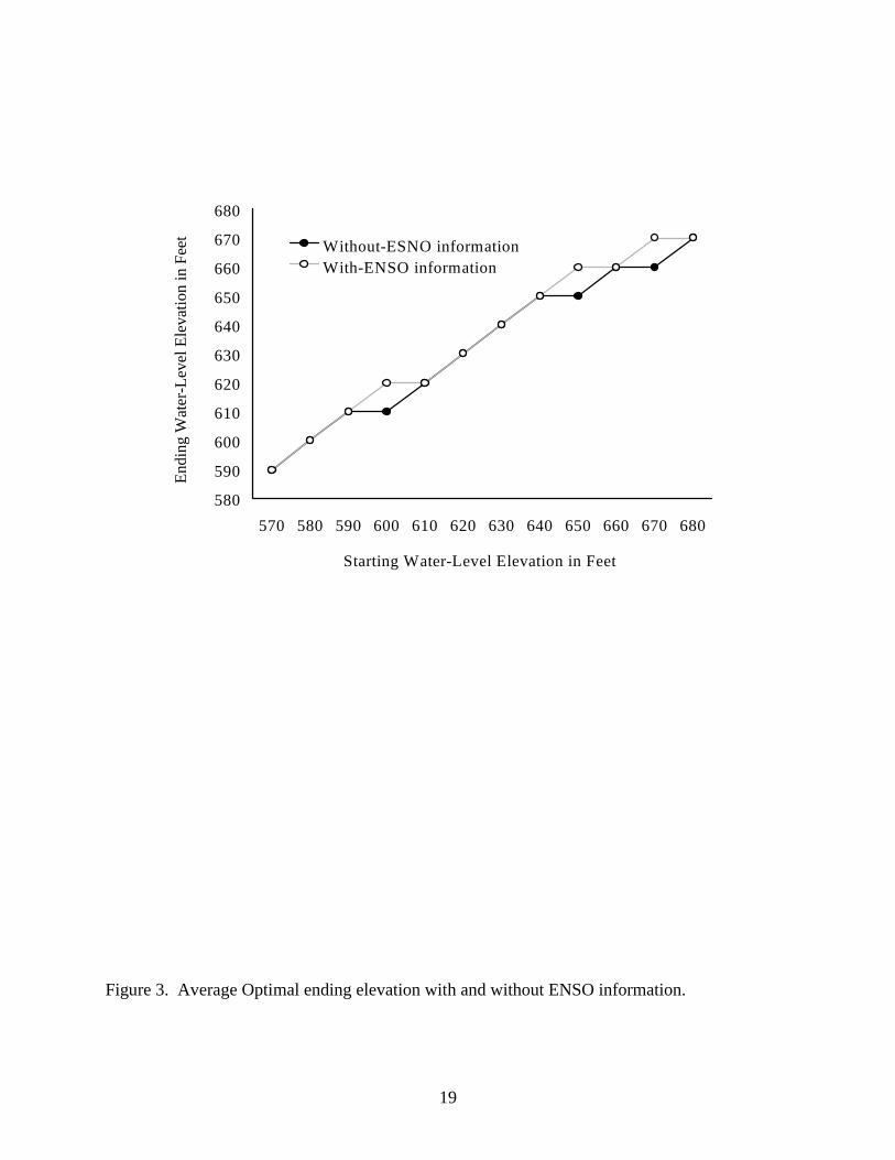
adjustment coming through the agricultural sector. In turn, ending water-level elevations rise

with incorporation of ENSO information results (Figure 3) and springflows are larger (Table 1).

The gains in elevation mainly occur under the El Niño and Neutral phases with average

management corresponding more to planning for La Niña and Neutral events. For example, at a

starting elevation of 620', the ending water-level elevation is at 640' with the El Niño phases

while the ending water-level elevation is at 630' with the La Niña phase (Figure 4). Note the

level of water use does not strongly depend on an initial water-level elevation. Rather, the

cutback in agricultural water use is roughly 20% across the board in all the elevation levels for

the La Niña and Neutral cases and about 5% in the El Niño case due to wetter conditions.

Table 2 presents the regional economic welfare implications of using ENSO information.

The welfare increase ranges from $1.1 to $3.5 million per year dependent on initial aquifer

elevation. Much of the welfare gain is captured by the agricultural sector due to the crop mix

and water use adjustments.

For sensitivity purposes the model was also run under the 400,000 af pumping limit that

EA usage is supposed to reach by year 2008 according to the Senate Bill 1477 (Table 3). Here,

as has been found in other studies, the principal adjustment occurs in agriculture [see McCarl et

15

al., 1998 for example]. Again, the use of ENSO information causes adjustments in the

agricultural sector and benefits that sector the most. Springflow at Comal Springs increases and

the chance of the springs going dry is reduced. Regional welfare gains are again positive but are

smaller than under the 450,000 af pumping limit case.

When the pumping limit is reduced to 400,000 af, the use of ENSO information helps to

offset losses in the agricultural sector. The value of ENSO forecast ranges from $2.5 million (at

the 600′ starting water-level elevation) to $3.5 million (at the 640′ starting water-level elevation)

under the 450,000 af pumping limit and ranges from $1.1 million (at the 660′ starting water-level

elevation) to $2.1 million (at the 640′ starting water-level elevation) under the 400,000 af

pumping limit.

9. Concluding Comments

This study investigates the regional benefits and water management actions that might

occur if the Edwards Aquifer water and agricultural management actions were conditioned on

ENSO phase information in the frequency that it existed from 1970-1996. Results show that

ENSO information does permit valuable adjustments worth $1.1 to $3.5 million depending on

Edwards Aquifer pumping limits and initial water-level elevations. The benefits and the bulk of

the water management adjustments largely involve shifts in agricultural crop mixes made to

exploit alterations in natural precipitation implied by the ENSO phases. The level of water use

does not strongly depend on an initial water-level elevation with the cutback in the agricultural

water use being roughly 20% across the board in all the elevation levels for the La Niña and

Neutral cases, and about 5% in the El Niño case due to wetter conditions. This indicates that it

would be desirable to promote the dissemination of ENSO information to agriculture along with

an education program on how to use such information. Non-agricultural sectors also exhibit

16

benefits due to reduced agricultural water use and increased spring flow. The exploitation of

ENSO information also reduces the regional welfare loss due to adoption of the legislatively

mandated regional aquifer pumping reduction.

Figu

Kerr

Edward

17

re 1. Hydrological boundaries of the Edwards Aquifer region

Texas

The Edwards AquiferRegion

Kinney Uvalde

Real

Medina

Bexar

Bandera

Kendall

San Antonio

Springs Recharge zone of the EA region

Hays

Comal

18

Figure 2. Cumulative probability of the Edwards Aquifer recharge for January to July, based on

October determination of the SOI phase

0.0

0.1

0.2

0.3

0.4

0.5

0.6

0.7

0.8

0.9

1.0

0 200 400 600 800 1000 1300 1800

El Nino PhaseLa Nina PhaseNeutral Phase

Prob

abili

ty o

f Rec

harg

e

Thousand Acre-Feet

19

Figure 3. Average Optimal ending elevation with and without ENSO information.

580

590

600

610

620

630

640

650

660

670

680

570 580 590 600 610 620 630 640 650 660 670 680

Without-ESNO informationWith-ENSO information

Endi

ng W

ater

-Lev

el E

leva

tion

in F

eet

Starting Water-Level Elevation in Feet

20

Figure 4. Average Optimal ending water-level elevations without ENSO information and with

El Niño and La Niña information

580

600

620

640

660

680

700

570 580 590 600 610 620 630 640 650 660 670 680

Without-ESNO informationEl Nino ForecastLa Nina Forecast

Endi

ng W

ater

-Lev

el E

leva

tion

in F

eet

Starting Water-Level Elevation in Feet

21

Table 1. Comparison of Average Base Scenario Hydrological Responses by Selected Starting

Elevation with and without ENSO Information

With ENSO Information Variable

Units Starting

Elevation No ENSO Information Average El Niño Neutral La Niña

Ending Elevation

End of year elevation at j-17 in feet

580 600 620 640 660

600 610 630 650 660

600 620 630 650 660

610 620 640 650 670

600 620 630 650 660

600 610 630 650 660

Comal Spring Flowa

1000 af of annual flow

580 600 620 640 660

0 0

66 144 209

0 0

-1 -4 -1

0 36 45 36 45

0 0

-8 -10 -8

0 0

-26 -27 -26

San Marcos Spring Flowa

1000 af of annual flow

580 600 620 640 660

49 56 64 72 79

-0.2 0.8

-0.2 -0.4 -0.2

14 14 14 13 14

-2 -1 -2 -2 -2

-9 -9 -9 -9 -9

Agricultural Pumping Water Usea

1000 af of annual use

580 600 620 640 660

136 139 139 128 140

-18 -29 -18 -13 -17

-24 -26 -25 -13 -26

-20 -33 -20

-15 -18

-7 -8 -8 -6 -7

Municipal and Industrial Pumping Water Usea

1000 af of annual use

580 600 620 640 660

303 304 303 300 303

1.2 -1.1 1.4 1.7 1.1

-1.8 1.0

-1.0 3.5

-0.2

0.8 -1.6 1.0 1.2 0.8

1.7 2.2 2.1

1.1 1.9

Total Pumping Water Usea

1000 af of annual use

580 600 620 640 660

439 443 442 428 443

-17 -30 -17 -11 -16

-26 -25 -26

-10 -26

-19 -34 -19

-14 -17

-5 -5 -6

-5 -5

a The information in the table associated with these rows in the with ENSO information columns

gives the change from the No ENSO information situation.

22

Table 2. Value of ENSO Information by Selected Starting Water-Level Elevation

450,000 af Pumping Limit 400,000 af Pumping Limit

Variable

Units

Starting Elevation

Without-ENSO Information

With-ENSO Information

Without-ENSO Information

With-ENSO Information

----- change from 450,000 without ENSO info case -----

Net Agricultural Income

1000 dollars 580 600 620 640 660

14,001 14,495 14,820 14,661 15,632

3,039 2,586 2,896 3,137 2,780

- 1,144 -1,586 -1,431 -1,147 -1,703

1,763 1,462 1,443 1,845 1,142

Net Municipal and Industrial Welfare

1000 dollars 580 600 620 640 660

617,047 617,332 617,555 617,469 618,071

77 -11 87 334 82

77 -143 89 240 88

-24 -122 -20 230 -27

Net Total Welfare 1000 dollars 580 600 620 640 660

631,049 631,828 632,375 632,130 633,703

3,116 2,575 2,983 3,471 2,862

-1,067 -1,729 - 1,342 -907 -1,615

1,739 1,340 1,423 2,075 1,115

23

Table 3. Comparison of Average Hydrological Responses by Selected Starting Elevation

under Different Water Management Strategy and with/without ENSO Information

450,000 af Pumping Limit

400,000 af Pumping Limit

Item Units

Starting Elevation

Without ENSO

Information

With ENSO

Information Without ENSO

Information with ENSO Information

-change from 450,000 without ENSO info case-- Ending Elevation

feet at j-17

580 600 620 640 660

600 610 630 650 660

10

10

10

Comal Flow

1000 af

580 600 620 640 660

0 0 66 144 209

0 0 -1 -4 -1

0 6 6 5 6

0 4 7 3 8

San Marcos Flow

1000 af

580 600 620 640 660

49 56 64 72 79

-0.2 0.8 -0.2 -0.4 -0.2

0.3 0.2 0.4 0.4 0.41

0.4 1.3 0.5 0.1 0.6

AG Water Use

1000 af

580 600 620 640 660

136 139 139 128 140

-18 -29 -18 -13 -17

- 46 - 45 - 45 - 33 - 45

-50 -54 -51 -40 -51

M&I Water Use

1000 af

580 600 620 640 660

303 304 303 300 303

1.2 -1.1 1.4 1.7 1.1

- 0.3 - 3.0 - 0.1 0.2 - 0.3

-2 -4 -2 -1 -2

Total Water Use

1000 af

580 600 620 640 660

439 443 442 428 443

-17 -30 -17 -11 -16

- 46 - 48 - 45 - 33 - 45

-52 -58 -53 -41 -53

24

References

Adams, R. M., K. J., Bryant, and B. A., McCarl, “Value of improved long range weather

information”, Contemporary Economics Policy, 13, 10-19, 1995.

Burt, O. R, “An economic control of groundwater reserves”, Journal of Farm Economics,

47, 324-346, 1966.

Burt, O. R, “An optimal resource use over time with an application to groundwater”,

Management Science, 11, 80-93, 1964.

Cayan, D. R., K. T. Redmond, and L. G. Riddle, “ENSO and hydrologic extremes in the

western United States”, Journal of Climate, 12, 2881-2893, 1999.

Chen, C. C., and B. A. McCarl, "The Value of ENSO Information to Agriculture:

Consideration of Event Strength and Trade", Journal of Agricultural and

Resource Economics, Vol. 25, no. 2 (December 2000):, 368-385, 2000.

Doorenbos, J., and W. O. Pruitt, Guidelines for Predicting Crop Water Requirements,

Food and Agriculture Organization of the United Nations, FAO Irrigation and

Drainage Paper, Rome, 1977.

Edwards Aquifer Authority, Homepage, http://www.e_aquifer.com, 1998.

Gershunov, A., “ENSO influence on intraseasonal extreme rainfall and temperature

frequencies in the contiguous United States: Implications for long_range

predictability”, Journal of Climate, 11, 3192-3203, 1998.

Griffin, R. C., and C. Chang, “Seasonality in community water demand”, Western

Journal of Agricultural Economics, 16, 207-217, 1991.

Heimes, F. J., and R. R. Luckey, Estimating 1980 groundwater pumpage for irrigation

on the high plains in parts of Colorado, Kansas, Nebraska, New Mexico,

Oklahoma, South Dakota, Texas, and Wyoming, USGS, Water Resources

Investigation Report 83-4123, Denver, Colorado, 1983.

Japan Meteorological Agency, http://www.kishou.go.jp/english/activities/observation

/obs5.html, 2001.

Keplinger, K. O., B. A. McCarl, M. Chowdury, and R. D. Lacewell, “Economic and

hydrologic implications of suspending irrigation in dry years”, Journal of

Agricultural and Resource Economics, 23, 191-205, 1998.

25

Kilmer, R. L., T. Spreen, and D. S. Tilley, “A dynamic plant location model: The East

Florida fresh citrus packing industry”, American Journal of Agricultural

Economics. 65, 730-37, 1984.

Longley, G., “The subterranean aquatic ecosystem of the balcones fault zone Edwards

aquifer in Texas - threats from overpumping”, in Proceedings of the First

International Conference on Ground Water Ecology, edited by J. A. Stanford, and

J. J. Simons, pp. 291-300, Tampa, Florida, 1992.

McCarl, B. A., “Cropping activities in agricultural sector models: A methodological

proposal”, American Journal of Agricultural Economics, 64, 768-72, 1982.

McCarl, B. A., K. O. Keplinger, C. Dillon, and R. L. Williams, “Limiting pumping from

the Edwards aquifer: An economic investigation of proposals, water markets and

springflow guarantees”, Water Resources Research, 35, 1257-1268, 1998.

McCarl, B. A., and T. H. Spreen “Price Endogenous Mathematical Programming as a

Tool for Sector Analysis”, American Journal of Agricultural Economics, 62, 87-

102, 1980.

McFarland, J., “Ground water management and salinity control: A case study in

Northwest Mexico”, American Journal of Agricultural Economics, 57, 456-62,

1975.

National Oceanic and Atmospheric Administration, Climatic Diagnostics Center,

http://www.cdc.noaa.gov/ENSO/enso.kd.html, 2000.

National Oceanic and Atmospheric Administration, National Climatic Data Center, El

Niño/La Niña: Depicting the Impacts of the 1997_2000 El Niño/La Niña,

http://www.ncdc.noaa.gov/ol/climate/elnino/elnino.html, 2000.

Sweeney, D., and R. Tathum, “An improved long run model of multiple warehouse

location”, Management Science, 22, 748-58, 1976.

Texas Legislature, Senate Bill No.1477, San Marcos/Comal Recovery Plan, 73rd Session,

Austin, Texas, 1993.

United States Fish and Wildlife Service, Albuquerque New Mexico, 1995.

United States Geological Survey, Recharge to and Discharge from the Edwards Aquifer

in the San Antonio Area, Texas, Austin, TX, various issues, the1997 report is on

http://tx.usgs.gov/reports/district/98/01/index.html.

26

Williams, R. L, Drought management and the Edwards aquifer: An economic inquiry,

Ph.D. dissertation, Department of Agricultural Economics, Texas A&M

University, College Station, Texas, 1996.

Williams, R. L., B. A. McCarl, and C. C. Chen, “Elevation dependent management of the

Edwards aquifer: A linked mathematical and dynamic programming approach”,

Working paper, Department of Agricultural Economics, Texas A&M University,

College Station, Texas, 2000.

Williams, J. R., C. A. Jones, J. R. Canaria, and D. A. Spaniel, “The EPIC crop growth

model”, Transactions of the American Society of Agricultural Engineers, 32, 497-

511, 1989.

Wurbs, R. A., Modeling and Analysis of Reservoir System Operations. N.J.: Prentice Hall,

1996, p. 356.