Ocean Sci., 9, 535–543, 2013www.ocean-sci.net/9/535/2013/doi:10.5194/os-9-535-2013© Author(s) 2013. CC Attribution 3.0 License.

EGU Journal Logos (RGB)

Advances in Geosciences

Open A

ccess

Natural Hazards and Earth System

Sciences

Open A

ccess

Annales Geophysicae

Open A

ccess

Nonlinear Processes in Geophysics

Open A

ccess

Atmospheric Chemistry

and Physics

Open A

ccess

Atmospheric Chemistry

and Physics

Open A

ccess

Discussions

Atmospheric Measurement

Techniques

Open A

ccess

Atmospheric Measurement

Techniques

Open A

ccess

Discussions

Biogeosciences

Open A

ccess

Open A

ccess

BiogeosciencesDiscussions

Climate of the Past

Open A

ccess

Open A

ccess

Climate of the Past

Discussions

Earth System Dynamics

Open A

ccess

Open A

ccess

Earth System Dynamics

Discussions

GeoscientificInstrumentation

Methods andData Systems

Open A

ccess

GeoscientificInstrumentation

Methods andData Systems

Open A

ccess

Discussions

GeoscientificModel Development

Open A

ccess

Open A

ccess

GeoscientificModel Development

Discussions

Hydrology and Earth System

Sciences

Open A

ccess

Hydrology and Earth System

Sciences

Open A

ccess

Discussions

Ocean Science

Open A

ccess

Open A

ccess

Ocean ScienceDiscussions

Solid Earth

Open A

ccess

Open A

ccess

Solid EarthDiscussions

The Cryosphere

Open A

ccess

Open A

ccess

The CryosphereDiscussions

Natural Hazards and Earth System

Sciences

Open A

ccess

Discussions

ENSO components of the Atlantic multidecadal oscillation and theirrelation to North Atlantic interannual coastal sea level anomalies

J. Park and G. Dusek

NOAA Center for Operational Oceanographic Products and Services 1305 East West Highway, Silver Spring, MD, USA

Correspondence to:J. Park (joseph.park@noaa.gov)

Received: 1 November 2012 – Published in Ocean Sci. Discuss.: 30 November 2012Revised: 26 April 2013 – Accepted: 13 May 2013 – Published: 10 June 2013

Abstract. The El Nino Southern Oscillation (ENSO) andthe Atlantic Multidecadal Oscillation (AMO) are known toinfluence coastal water levels along the East Coast of theUnited States. By identifying empirical orthogonal functions(EOFs), which coherently contribute from the MultivariateENSO Index (MEI) to the AMO index (AMOI), we char-acterize both the expression of ENSO in the unsmoothedAMOI, and coherent relationships between these indices andinterannual sea level anomalies at six stations in the Gulf ofMexico and western North Atlantic. Within the ENSO band(2–7 yr periods) the total contribution of MEI to unsmoothedAMOI variability is 79 %. Cross correlation suggests that theMEI leads expression of the ENSO signature in the AMOI bysix months, consistent with the mechanism of an atmosphericbridge. Within the ENSO band, essentially all of the cou-pling between the unsmoothed AMOI and sea level anoma-lies is the result of ENSO expression in the AMOI. At longerperiods we find decadal components of sea level anomalieslinked to the AMOI at three southern stations (Key West,Pensacola, Charleston), but not at the northern stations (Bal-timore, Boston, Portland), with values of coherence rangingfrom 20 to 50 %. The coherence of MEI to coastal sea levelanomalies has a different structure and is generally weakerthan that of the ENSO expressed AMOI influence, suggest-ing distinct physical mechanisms are influencing sea levelanomalies due to a direct ENSO teleconnection when com-pared to teleconnections based on ENSO expression in theAMOI. It is expected that applying this analysis to extremesof sea level anomalies will reveal additional influences.

1 Introduction

The El Nino Southern Oscillation (ENSO) has been identi-fied as an important forcing on sea level anomalies of thewestern Pacific Ocean and the west coast of the United States(Sweet et al., 2009). Along the east coast of the United Statesstorm surges have a positive correlation with the El Ninophase of ENSO where patterns of anomalously high sea lev-els are attributed to El Nino related changes in atmosphericpressure over the Gulf of Mexico and eastern Canada, andto the wind field over the continental shelf of the northeastUnited States (Sweet and Zervas, 2011). The Atlantic Mul-tidecadal Oscillation (AMO) has received less attention inrelation to sea level anomalies, but has been related to coher-ent sea surface height variability along the western boundaryof the North Atlantic (Frankcombe and Dijkstra, 2009), to re-gional variability of coastal sea levels along the mid-Atlanticcoast (Sallenger et al., 2012) and to extreme sea levels alongthe coast of Florida (Park et al., 2010).

The dominant period of leading empirical orthogonalfunctions (EOFs) of ENSO and AMO are roughly an order ofmagnitude different: 5.1 yr for the leading mode of the Mul-tivariate ENSO Index (MEI) and roughly 70 yr for the lead-ing mode of the AMO index (AMOI). The first EOF of theAMOI closely matches a ten-year (121 month) moving aver-age of the unsmoothed AMOI and effectively ignores inter-annual processes, however, the unsmoothed AMOI exhibitsamplitude modulations at periods of roughly 3 to 7 yr (as dis-cussed below and illustrated in Fig. 1).

That ENSO has a signature in the AMO is not surpris-ing, and progress has been made relating the degree of thisteleconnection. For example, Guan and Nigam (2009) an-alyzed twentieth century Atlantic sea surface temperature

Published by Copernicus Publications on behalf of the European Geosciences Union.

536 J. Park and G. Dusek: ENSO components of the Atlantic multidecadal oscillation

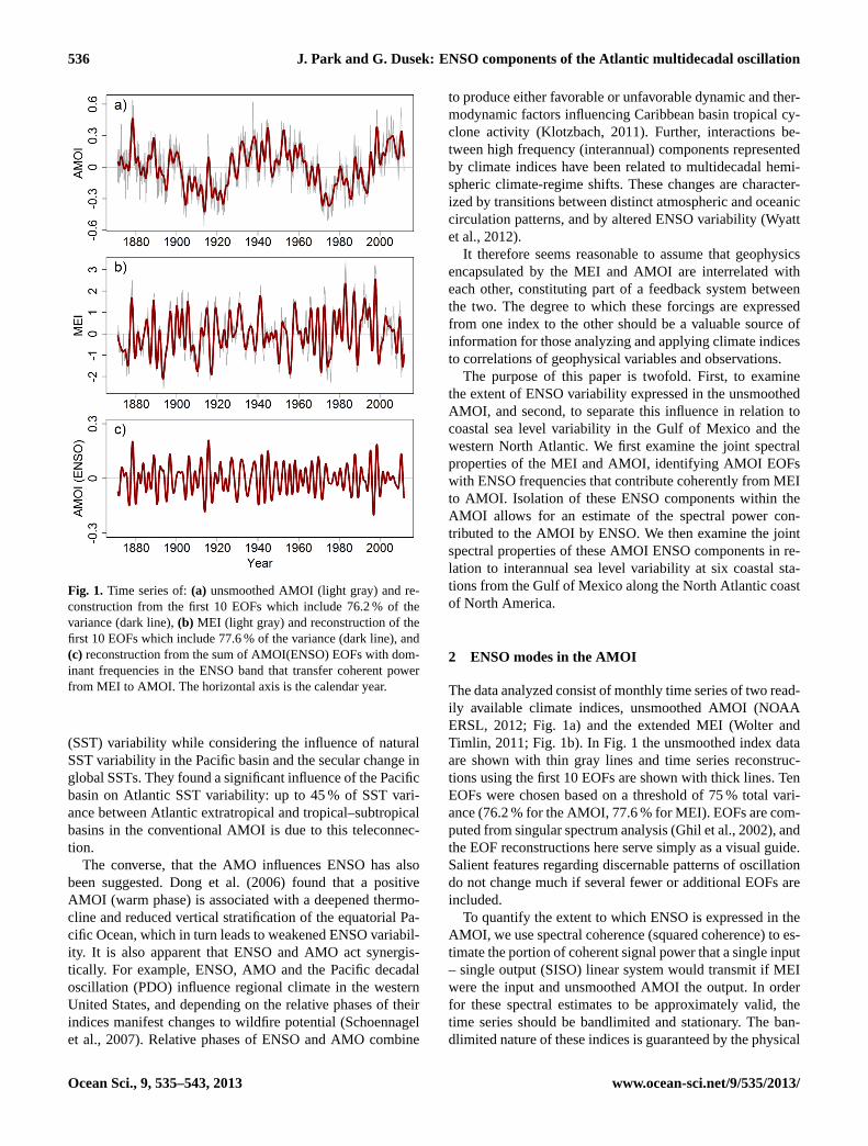
Fig. 1. Time series of:(a) unsmoothed AMOI (light gray) and re-construction from the first 10 EOFs which include 76.2 % of thevariance (dark line),(b) MEI (light gray) and reconstruction of thefirst 10 EOFs which include 77.6 % of the variance (dark line), and(c) reconstruction from the sum of AMOI(ENSO) EOFs with dom-inant frequencies in the ENSO band that transfer coherent powerfrom MEI to AMOI. The horizontal axis is the calendar year.

(SST) variability while considering the influence of naturalSST variability in the Pacific basin and the secular change inglobal SSTs. They found a significant influence of the Pacificbasin on Atlantic SST variability: up to 45 % of SST vari-ance between Atlantic extratropical and tropical–subtropicalbasins in the conventional AMOI is due to this teleconnec-tion.

The converse, that the AMO influences ENSO has alsobeen suggested. Dong et al. (2006) found that a positiveAMOI (warm phase) is associated with a deepened thermo-cline and reduced vertical stratification of the equatorial Pa-cific Ocean, which in turn leads to weakened ENSO variabil-ity. It is also apparent that ENSO and AMO act synergis-tically. For example, ENSO, AMO and the Pacific decadaloscillation (PDO) influence regional climate in the westernUnited States, and depending on the relative phases of theirindices manifest changes to wildfire potential (Schoennagelet al., 2007). Relative phases of ENSO and AMO combine

to produce either favorable or unfavorable dynamic and ther-modynamic factors influencing Caribbean basin tropical cy-clone activity (Klotzbach, 2011). Further, interactions be-tween high frequency (interannual) components representedby climate indices have been related to multidecadal hemi-spheric climate-regime shifts. These changes are character-ized by transitions between distinct atmospheric and oceaniccirculation patterns, and by altered ENSO variability (Wyattet al., 2012).

It therefore seems reasonable to assume that geophysicsencapsulated by the MEI and AMOI are interrelated witheach other, constituting part of a feedback system betweenthe two. The degree to which these forcings are expressedfrom one index to the other should be a valuable source ofinformation for those analyzing and applying climate indicesto correlations of geophysical variables and observations.

The purpose of this paper is twofold. First, to examinethe extent of ENSO variability expressed in the unsmoothedAMOI, and second, to separate this influence in relation tocoastal sea level variability in the Gulf of Mexico and thewestern North Atlantic. We first examine the joint spectralproperties of the MEI and AMOI, identifying AMOI EOFswith ENSO frequencies that contribute coherently from MEIto AMOI. Isolation of these ENSO components within theAMOI allows for an estimate of the spectral power con-tributed to the AMOI by ENSO. We then examine the jointspectral properties of these AMOI ENSO components in re-lation to interannual sea level variability at six coastal sta-tions from the Gulf of Mexico along the North Atlantic coastof North America.

2 ENSO modes in the AMOI

The data analyzed consist of monthly time series of two read-ily available climate indices, unsmoothed AMOI (NOAAERSL, 2012; Fig. 1a) and the extended MEI (Wolter andTimlin, 2011; Fig. 1b). In Fig. 1 the unsmoothed index dataare shown with thin gray lines and time series reconstruc-tions using the first 10 EOFs are shown with thick lines. TenEOFs were chosen based on a threshold of 75 % total vari-ance (76.2 % for the AMOI, 77.6 % for MEI). EOFs are com-puted from singular spectrum analysis (Ghil et al., 2002), andthe EOF reconstructions here serve simply as a visual guide.Salient features regarding discernable patterns of oscillationdo not change much if several fewer or additional EOFs areincluded.

To quantify the extent to which ENSO is expressed in theAMOI, we use spectral coherence (squared coherence) to es-timate the portion of coherent signal power that a single input– single output (SISO) linear system would transmit if MEIwere the input and unsmoothed AMOI the output. In orderfor these spectral estimates to be approximately valid, thetime series should be bandlimited and stationary. The ban-dlimited nature of these indices is guaranteed by the physical

Ocean Sci., 9, 535–543, 2013 www.ocean-sci.net/9/535/2013/

J. Park and G. Dusek: ENSO components of the Atlantic multidecadal oscillation 537

Table 1. AMOI(ENSO) EOFs with dominant frequencies in theENSO band (2 to 7 yr) that contribute coherent power from the MEIto AMOI.

EOF Rank 5 6 7 8 9 10

Period (yr) 3.51 3.60 5.14 4.97 2.82 2.57Variance (%) 3.1 3.0 2.9 2.7 2.4 2.2

variables upon which they are computed, large-scale geo-physical processes with inertia and damping that precludestep or delta function components. To assess stationarity, weapplied the augmented Dickey–Fuller test to both the un-smoothed AMOI and MEI, and found the null hypothesis ofa unit root in the characteristic equation for each time seriesrejected at the 99 % confidence level.

To identify AMOI EOFs with coherent power between theMEI and AMOI, which we denote AMOI(ENSO) modes,we first select AMOI EOFs that have a dominant spectralpeak in the ENSO band, resulting in seven modes with EOFeigenvalue ranks (based on decreasing partial variance) of 5,6, 7, 8, 9, 10 and 11. The next criteria quantifies the extentto which linear combinations of these modes contribute co-herent power from the MEI to the AMOI. We evaluate thisby maximizing the reduction in total coherence between theMEI and AMOI with sequential removal of all possible lin-ear combinations of the seven AMOI EOFs with a dominantspectral peak in the ENSO band.

To estimate the fraction of coherent power reduction,R,we compute the ratio of the integral of coherence betweenthe two models:

Ri = 1−

∫γ 2

MAE(i)df

/∫γ 2

MA df , (1)

whereγ 2MA is the coherence function of MEI to unsmoothed

AMOI (Fig. 2, blue line), andγ 2MAE(i) is the coherence func-

tion between MEI and the AMOI EOF reconstruction minusthei-th linear combination of the prospective AMOI(ENSO)modes. The limits of integration are the ENSO band peri-ods from 2 to 7 yr. With seven prospective modes (EOFs 5to 11) there are 127 combinations, and we select the com-bination of modes that maximizes the coherence reductionwith the result that removal of the six AMOI EOFs 5, 6, 7,8, 9, and 10, produces a maximal reduction ofR = 79.0 %across the ENSO band. This indicates that EOF 11 (with aperiod of 2.25 yr and comprising 2.1 % of the AMOI vari-ance) is not contributing coherently between the MEI andAMOI. We therefore identify the six modes listed in Table 1as the AMOI(ENSO) modes.

Figure 1c plots a time series reconstruction from these sixAMOI(ENSO) EOFs. Inspection of Fig. 1 reveals an uneventransmission of MEI variability to the AMOI(ENSO) recon-struction as a function of time. For example, around the year1945 the MEI (Fig. 1b) presents relatively little variability,

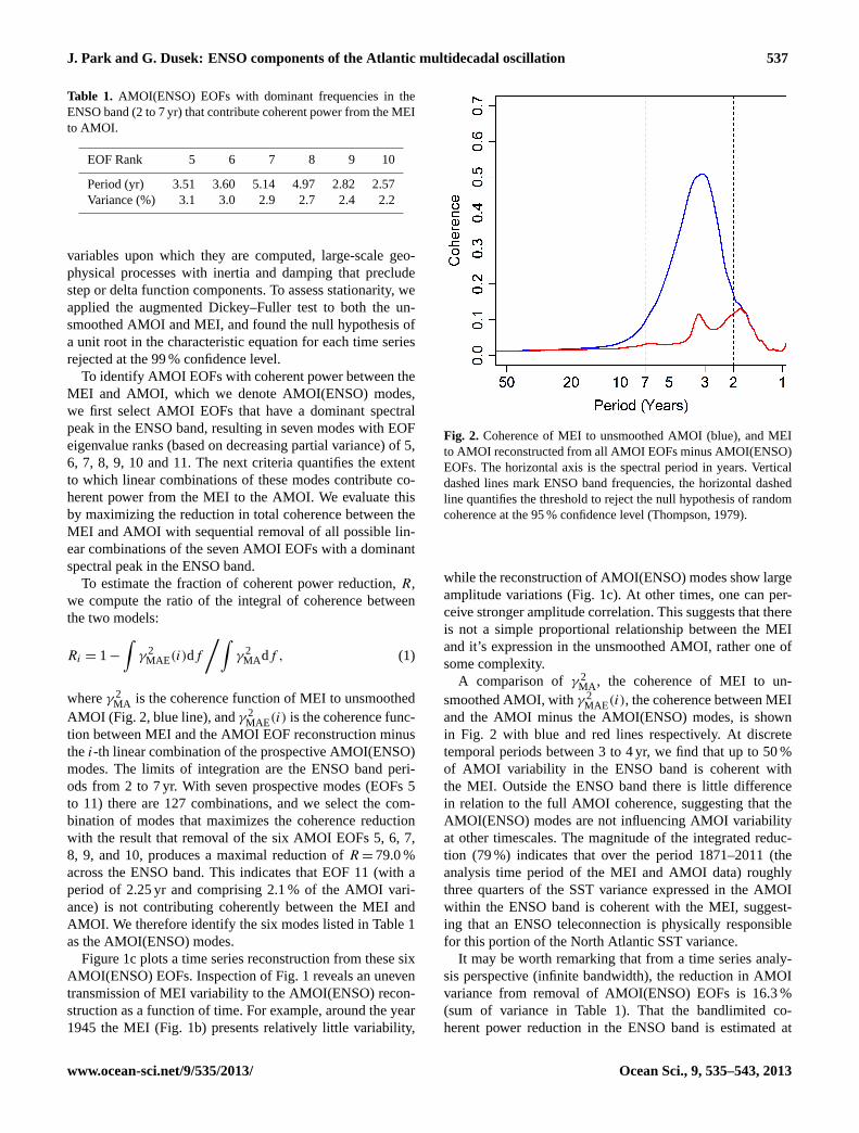
Fig. 2. Coherence of MEI to unsmoothed AMOI (blue), and MEIto AMOI reconstructed from all AMOI EOFs minus AMOI(ENSO)EOFs. The horizontal axis is the spectral period in years. Verticaldashed lines mark ENSO band frequencies, the horizontal dashedline quantifies the threshold to reject the null hypothesis of randomcoherence at the 95 % confidence level (Thompson, 1979).

while the reconstruction of AMOI(ENSO) modes show largeamplitude variations (Fig. 1c). At other times, one can per-ceive stronger amplitude correlation. This suggests that thereis not a simple proportional relationship between the MEIand it’s expression in the unsmoothed AMOI, rather one ofsome complexity.

A comparison ofγ 2MA , the coherence of MEI to un-

smoothed AMOI, withγ 2MAE(i), the coherence between MEI

and the AMOI minus the AMOI(ENSO) modes, is shownin Fig. 2 with blue and red lines respectively. At discretetemporal periods between 3 to 4 yr, we find that up to 50 %of AMOI variability in the ENSO band is coherent withthe MEI. Outside the ENSO band there is little differencein relation to the full AMOI coherence, suggesting that theAMOI(ENSO) modes are not influencing AMOI variabilityat other timescales. The magnitude of the integrated reduc-tion (79 %) indicates that over the period 1871–2011 (theanalysis time period of the MEI and AMOI data) roughlythree quarters of the SST variance expressed in the AMOIwithin the ENSO band is coherent with the MEI, suggest-ing that an ENSO teleconnection is physically responsiblefor this portion of the North Atlantic SST variance.

It may be worth remarking that from a time series analy-sis perspective (infinite bandwidth), the reduction in AMOIvariance from removal of AMOI(ENSO) EOFs is 16.3 %(sum of variance in Table 1). That the bandlimited co-herent power reduction in the ENSO band is estimated at

www.ocean-sci.net/9/535/2013/ Ocean Sci., 9, 535–543, 2013

538 J. Park and G. Dusek: ENSO components of the Atlantic multidecadal oscillation

79 % implies that 0.790× 0.163= 12.9 % of the time se-ries variance is attributed to the AMOI(ENSO) EOFs, while16.3–12.9= 3.4 % are contributions from AMOI(ENSO)EOFs at frequencies outside the ENSO band.

Power spectral density estimates computed with smoothedperiodograms of the three signals shown in Fig. 1 are pre-sented in Fig. 3, and provide a basis for comparison withspectral characteristics of the sea level anomalies. As ex-pected, the AMOI has the greatest power at multidecadalperiods in excess of 20 yr. Interesting features include theband of enhanced variability around a period of 10 yr, andthe smaller, smooth peaks between 3 and 6 yr that are similarto features in the MEI spectrum. The MEI spectrum charac-teristically reveals peak power in the ENSO band, while theAMOI(ENSO) spectrum presents a prominent energy distri-bution across the ENSO band as well as a significant but lowpower component with an annual period. (This annual com-ponent is 40 dB below the ENSO band peak amplitude, a ra-tio of 1E-4.) Since the AMOI(ENSO) EOFs were selectedonly if their dominant spectral component was within theband from 2 to 7 yr, we conclude that this low amplitude an-nual component represents a linear superposition of low en-ergy components from two or more of the six AMOI(ENSO)EOFs.

In addition to the mean spectral power conveyed from theMEI to the AMOI, the average temporal relationship betweenthe two is of interest. Figure 4 plots the cross-correlationfunction between MEI and AMOI(ENSO) EOFs, and we findthat MEI leads the expression of ENSO in the AMOI by anaverage of 6 months. Potential mechanisms for this correla-tion are discussed below.

3 Interannual sea level anomalies

Having suggested that ENSO influence on the AMOI can beestimated with spectral coherence, and in light of the factthat sea level anomalies in the western North Atlantic are in-fluenced by both ENSO and AMO, we would like to probethe extent to which these influences can be separated in re-lation to western North Atlantic coastal sea level variability.We examine monthly mean sea level anomalies at six long-term tidal gauges in the Gulf of Mexico and along the easternseaboard of the United States (Fig. 5). Table 2 lists the sta-tions along with the period of record for each station, andFig. 6 plots the anomalies computed from monthly mean sealevels with the average seasonal cycle and linear sea leveltrend removed (Zervas, 2009; NOAA CO-OPS, 2012).

To establish perspective on the spectral distribution ofthese anomalies, power spectral density estimates for eachof the time series in Fig. 6 are shown in Fig. 7. All sta-tions are dominated by variance at the decadal and longertimescales, with interannual and ENSO band power compo-nents also apparent. However, it is difficult to identify clearattributes in spectral variance with respect to either ENSO or

Fig. 3. Power spectral density estimates of(a) unsmoothed AMOI,(b) MEI, and(c) reconstruction of the sum of the six AMOI EOFswith dominant frequencies in the ENSO band that contribute coher-ently from MEI to AMOI. The horizontal axis is the spectral periodin years. Vertical dashed lines mark ENSO band frequencies, verti-cal bar quantifies the 95 % confidence interval.

Table 2.Tidal stations and period of record.

Station Period of record

Pensacola, FL January 1924–December 2011Key West, FL January 1913–December 2011Charleston, SC January 1922–December 2011Baltimore, MD January 1903–December 2011Boston, MA January 1921–December 2011Portland, ME January 1912–December 2011

AMO forcings. We will again use a SISO spectral coherencemodel to estimate the relative forcings between MEI, AMOIand AMOI(ENSO) as inputs, and the sea level anomalies asoutput.

Coherence between the unsmoothed AMOI and sea levelanomalies are presented in Fig. 8 with blue lines, and be-tween reconstructions based on AMOI(ENSO) EOFs and sealevel anomalies in red. The horizontal dashed line quantifies

Ocean Sci., 9, 535–543, 2013 www.ocean-sci.net/9/535/2013/

J. Park and G. Dusek: ENSO components of the Atlantic multidecadal oscillation 539

Fig. 4. Cross correlation between MEI and reconstruction from thesix AMOI(ENSO) EOFs. The peak correlation value is 0.47 withMEI leading AMOI by 6 months. Dashed lines quantify 95 % con-fidence intervals outside of which the null hypothesis of zero corre-lation is rejected.

Fig. 5.Map of the six tidal stations.

the threshold to reject the null hypothesis of random coher-ence at the 95 % confidence level (Thompson, 1979). At pe-riods from 6 to 15 yr, with a peak near 9 yr, there is evi-dence of weak AMOI coupling at Key West, Pensacola andCharleston. Estimates of the coherence reduction betweenAMOI and AMOI(ENSO) forcings integrated over periodsfrom 6 to 15 yr are 86.8, 85.9 and 97.9 % respectively. These

Fig. 6. Interannual variation of monthly mean sea level (gray line)at six long-term tidal stations along the east coast of the UnitedStates. The average seasonal cycle and linear sea level trend havebeen removed. A six month moving average is shown with the thickline. The horizontal axis is the calendar year.

large reductions indicate that mechanisms related to AtlanticSST (as expressed in the AMOI), which arenot being in-fluenced by ENSO, are coherent with decadal variability ofsea level anomalies at these three southeastern US stations.Within the limitations of a SISO model, the estimate of peakcoherence at these stations is roughly 0.2 at Key West andPensacola, and 0.3 at Charleston, suggesting that the fractionof sea level anomaly variance at a period of 9 yr driven bynon-ENSO forcings expressed in the AMOI are between 20to 30 %.

Moving to periods from 4 to 2.6 yr, we observe broad-band coherence centered at 2.8 yr at Charleston, and a cou-pling centered at 3.2 yr at Boston and Portland, althoughthe Boston forcing is less distinct than at Portland. Coher-ence at all three stations is essentially equivalent between theAMOI and AMOI(ENSO) forcings of sea level anomalies,leading to the conclusion that over this frequency band sealevel anomalies coherent with the AMOI are also coherentwith the MEI, which is being expressed in AMOI. Thus we

www.ocean-sci.net/9/535/2013/ Ocean Sci., 9, 535–543, 2013

540 J. Park and G. Dusek: ENSO components of the Atlantic multidecadal oscillation

Fig. 7. Power spectral density estimates of interannual sea levelvariations at six long-term tidal stations along the east coast of theUnited States. The horizontal axis is the spectral period in years.Vertical dashed lines mark ENSO band frequencies, vertical barquantifies the 95 % confidence interval.

conjecture that ENSO forcings expressed in the AMOI arethe drivers of this variability.

The next frequency band of interest covers periods from2.6 to 1.8 yr, for which there are prominent peaks centered at2.2 yr at Portland, Boston and Baltimore, with less distinctcouplings exhibited at Charleston and Pensacola. Each ofthese couplings shows nearly equivalent coherence whetherAMOI or AMOI(ENSO) forcings are considered, again re-vealing sea level anomalies at these stations coherent withAMOI are also coherent with ENSO modes expressed in theAMOI. The estimate of coherence at the 2.2 yr period peak is0.4 at Baltimore and Portland, and 0.5 at Boston, indicatingthat 40 to 50 % of the anomaly variance at this period is be-ing forced by a mechanism expressed in the AMOI but dueto ENSO forcing.

The final band with generally common features amongthe stations covers periods from 1.8 to 1.3 yr, with a peakcoherence near 1.5 yr. Here, we find conflicting results inthe sense that at Key West, Pensacola, Baltimore and Port-land the AMOI coupling to sea level anomalies is stronger

Fig. 8. Coherence between AMOI and interannual sea level vari-ations (blue), and coherence between the reconstruction from theAMOI(ENSO) and interannual sea level variations (red). The hori-zontal axis is the spectral period in years. Vertical dashed lines markENSO band frequencies, the horizontal dashed line quantifies thethreshold to reject the null hypothesis of random coherence at the95 % confidence level (Thompson, 1979).

than the AMOI(ENSO) expression, while at Charleston theAMOI(ENSO) is stronger, and at Boston the coherence isroughly equivalent. We will discuss these conflicts below.

In addition to AMOI and AMOI(ENSO) couplings to sealevel anomalies, we also examine direct ENSO influence byestimating MEI to sea level anomaly coherence as shownin Fig. 9 (green line). For comparison, coherence betweenAMOI(ENSO) EOFs and the anomalies are shown in red(same curve as Fig. 8). The most prominent feature is theMEI to sea level anomaly coherence at Key West centeredon a period of 7 yr, although the peak coherence is weak at0.26. Since coherence between AMOI(ENSO) and the sealevel anomaly response is near zero (red line), the analysissuggests this component of sea level variability is coupled toENSO forcings that are not expressed in the AMOI, for ex-ample, atmospheric pressure changes not reflected in NorthAtlantic SST.

Ocean Sci., 9, 535–543, 2013 www.ocean-sci.net/9/535/2013/

J. Park and G. Dusek: ENSO components of the Atlantic multidecadal oscillation 541

Fig. 9. Coherence between MEI and interannual sea level vari-ations (green), and coherence between the reconstruction fromAMOI(ENSO) EOFs and interannual sea level variations (red). Thehorizontal axis is the spectral period in years. Vertical dashed linesmark ENSO band frequencies, the horizontal dashed line quantifiesthe threshold to reject the null hypothesis of random coherence atthe 95 % confidence level (Thompson, 1979).

At Pensacola there is no evidence of MEI coupling tosea level anomalies, and in general the other stations exhibitweak coherence across the ENSO band. To the extent thatthese weak forcings have physical significance, the observa-tion that the spectral shape and location of peaks betweenthe MEI coherent (green) and AMOI(ENSO) coherent (red)curves do not generally coincide in frequency suggests thatthere are distinct geophysical forcings at work. Again, onemight speculate that directly coupled MEI modes are influ-enced by ENSO driven atmospheric teleconnections, whichare not expressed in the AMOI, while the AMOI(ENSO) re-lated anomalies are coupled to ENSO forcings, which are ex-pressed in Atlantic SST variability.

It is worth recalling that previous analysis of ENSO-forcedsea level anomalies in the western North Atlantic found cou-plings between ENSO and storm surges, the extreme valuesof sea level anomalies (Sweet and Zervas, 2011). Thus weexpect more significant results would be obtained in relation

to MEI influence on the extreme sea level anomalies ratherthan on the anomalies themselves.

4 Discussion

When viewed within the constraints of a SISO linear systemsmodel 40 to 50 % of unsmoothed AMOI variability is coher-ent with the MEI at periods between 2.5 and 4 yr (Fig. 2). Byexamining AMOI EOFs with dominant spectral frequenciesin the ENSO band and which contribute coherently from theMEI to AMOI, we identified six AMOI EOFs that expressAtlantic SST variance in response to ENSO related forcing.When these six AMOI(ENSO) EOFs are removed from theAMOI reconstruction, there is a 79 % reduction in total co-herent power between the MEI and AMOI (integrated overperiods from 2 to 7 yr). Thus we are led to the conclusionthat ENSO influences are expressed with some vigor in theunsmoothed AMOI, consistent with the findings of Guan andNigam (2009). To the extent that the SISO model capturesteleconnections between ENSO and Atlantic SST variabil-ity, one might expect a similar magnitude of expression inENSO forced Atlantic SST geophysical dynamics, that overthe ENSO band roughly three fourths of the total varianceexpressed in Atlantic SST forced dynamics are forced byENSO variability.

In the time domain, cross correlation between the MEI andreconstruction of the AMOI(ENSO) EOFs finds MEI leadingexpression in the AMOI with a 6 month lead time (Fig. 4).This is consistent with a six month lag reported by Gamiz-Fortis et al. (2011) between single EOFs of North AtlanticSST and the Bivariate ENSO index with 3.6 yr oscillatoryperiod, as well as with lag times characteristic of an ENSOatmospheric bridge (Klein et al., 1999). Thus we expect thedominant forcing expressed in AMOI within the ENSO bandcorresponds to anomalies in atmospheric circulation associ-ated with ENSO, which induce changes in the evaporationand cloud cover that, in turn, alter the net heat flux enteringthe North Atlantic (Klein et al., 1999).

Given that ENSO and AMO influence coastal sea levelanomalies of the western North Atlantic (Sweet and Zervas,2011; Frankcombe and Dijkstra, 2009; Park et al., 2010),and having identified ENSO forced modes of the AMOI, onecan separate influences from ENSO forced AMOI; AMOI;and MEI to these anomalies. Concerning AMOI couplingwithout ENSO forcing, we find evidence that Atlantic SSTvariability as expressed in the unsmoothed AMOI is par-tially coherent with coastal sea level anomalies in a broad-band centered on a period near 9 yr at the three southernstations of Key West, Pensacola and Charleston. The peakstrength of this forcing varies from 20 to 30 %, and wenote that this energy is apparent in the power spectral es-timate of the unsmoothed AMOI (Fig. 3). Since Pensacolais located within the northern Gulf of Mexico it shouldnot be directly influenced by Atlantic meridonal overturning

www.ocean-sci.net/9/535/2013/ Ocean Sci., 9, 535–543, 2013

542 J. Park and G. Dusek: ENSO components of the Atlantic multidecadal oscillation

circulation (AMOC), which has been linked to AMO vari-ability (Zhang, 2008), or by changes in coastal sea levels at-tributed to geostrophic relaxation of Gulf Stream transport(Noble and Gelfenbaum, 1992). Therefore, one can specu-late that this coupling reflects an atmospheric teleconnec-tion expressed in the Atlantic SST, which is coherent withcoastal sea level anomalies at these three stations. Arguezet al. (2009) observed modes in both AMOI and the NorthAtlantic Oscillation (NAO) index with periods of approxi-mately 10 yr, suggesting a component of decadal variabilityin North Atlantic SST from atmospheric forcing. However,their analysis finds maximal correlation between NAO andNorth Atlantic SST anomalies from North Carolina to NovaScotia, with essentially no link south of Charleston. Since the9 yr modes coherent between AMOI and sea level anomaliesshown in Fig. 8 are found only at the three southern stations,and not at the mid-Atlantic and northern stations, we suspectthat the NAO is not a causative mechanism for these decadalsea level anomalies.

Regarding ENSO coupled Atlantic SST variability in-fluencing coastal sea level anomalies, coherence betweenAMOI(ENSO) EOFs and anomalies at the six stations sup-port two main conclusions. First, within the ENSO band (pe-riods of 2 to 7 yr) essentially all of the forcing identified be-tween unsmoothed AMOI and sea level anomalies are theresult of ENSO expression in the AMOI. This can be seenin the overlap of the unsmoothed AMOI and AMOI(ENSO)coherence functions within the ENSO band (Fig. 8). Second,three broadband couplings centered at periods of 3.2, 2.8 and2.2 yr are presented in varying strength across the six sta-tions. Specifically, the 3.2 yr forcing is evidenced at Bostonand Portland, the 2.8 yr mode at Charleston, and the 2.2 yrcoupling at all stations except Key West.

At periods shorter than the ENSO band, persistent cou-pling is found to some degree at all stations near a periodof 1.5 yr. This coupling is not consistently represented as be-ing forced by either AMOI or AMOI(ENSO). It seems likelythat the SISO model fails to account for influences other thanENSO or Atlantic SST variability at this period. For exam-ple, coastal sea levels at a specific station reflect oceano-graphic and climatological forcings not captured in the MEIor AMOI. Another potential influence is barometric effectsand associated climatological changes related to storms asexpressed in the NAO index, which has been correlated withwestern North Atlantic interannaul sea levels (Papadopoulosand Tsimplis, 2006). It is also known that changes in volumetransport of the Gulf Stream impact the geostrophic balanceof coastal sea levels along the western Atlantic on seasonaland interannual timescales (Noble and Gelfenbaum, 1992).Additionally, recent work by Wyatt et al. (2012) finds thatshorter-term, interannual to interdecadal climate variabilityalters character according to polarity of their “stadium wave”hemispheric interaction, and suggest that mutual interactionbetween shorter-term variability and the stadium wave im-

pacts interannual and multidecadal variability within the At-lantic sector.

When we examine direct MEI to sea level anomaly coher-ence, the coupling is generally weak and in most cases ex-pressed with different spectral shapes than for either the di-rect AMOI or AMOI(ENSO) influences. We therefore spec-ulate that there are distinct physical mechanisms driving thesea level anomalies coherent with the AMOI(ENSO) modesfrom those coherent directly with MEI. That the MEI cou-plings are weaker than those of the AMOI(ENSO) modeshints that ENSO influenced teleconnections that are relatedto SST variance have a stronger coupling to North Atlanticsea level anomalies than ENSO teleconnections not relatedto SST. We also note that analysis based on the extreme val-ues of the sea level anomalies (storm surges) is likely to finda stronger influence from direct MEI coupling (Sweet andZervas, 2011).

As noted by Wyatt et al. (2012), advantages of analyz-ing climate indices rather than unsmoothed observationalvariables include increased dynamical interpretability, in-creased signal-to-noise ratio and statistical significance, al-beit at the expense of phenomenological completeness. Thisdecoupling from raw fields limits our capability to engagein speculation regarding geophysical connections for the ob-served forcings. Further, the links we identified are limitedto a few geospatial locations responding to synoptic-scaleforcings captured by the indices. Clarification of the struc-ture of these links and their attribution will involve the ap-plication of global climate models that capture the coupledocean–atmosphere geophysical feedbacks.

5 Conclusion

We have assumed that a linear systems transfer function ex-ists between the MEI and AMOI, and argued that since theseindices are bandlimited and quasi-stationary, the spectral co-herence provides a first-order estimate of coupling betweenthe MEI and AMOI. However, if there is a physically basedtransfer function between these two indices it is likely non-linear and further, it is nearly certain that a single input–single output model is insufficient to capture the inherentdynamics. Therefore, work remains to further explore theseissues and clarify the decomposition of teleconnections be-tween the two. Nonetheless, we believe that these results pro-vide progress in that direction.

Identification of unsmoothed AMOI EOFs with dominantspectral periods in the ENSO band that contribute coherentlyfrom the MEI to AMOI allows us to isolate ENSO modesexpressed in the AMOI. The results indicate that about threequarters (79 %) of the total coherent signal power in theENSO band of the unsmoothed AMOI is attributed to forc-ing from the MEI, while couplings in the range of 40 to 50 %can be found at discrete periods between 2.5 to 4 yr. Froma temporal perspective, we find that the MEI forcing leads

Ocean Sci., 9, 535–543, 2013 www.ocean-sci.net/9/535/2013/

J. Park and G. Dusek: ENSO components of the Atlantic multidecadal oscillation 543

the unsmoothed AMOI response by an average of 6 months,characteristic of an ENSO atmospheric bridge.

Comparison of coherence spectra between AMOI(ENSO)EOFs and monthly sea level anomalies to coherence be-tween unsmoothed AMOI and sea level anomalies, allowsus to separate influences of ENSO coupled Atlantic SSTanomalies from those that are not ENSO related. We findthat three southern stations (Key West, Pensacola andCharleston) exhibit an AMOI to sea level anomaly responsecentered near a period of 9 yr, that ENSO forcings are notexpressed in these AMOI influenced variations, and they donot seem consistent with NAO coupling. Within the ENSOband nearly all of the sea level anomaly variations thatare coherent with AMOI are coherent with AMOI(ENSO)modes, accounting for 20 to 50 % of the sea level anomalyvariance. This suggests that ENSO forcing is acting throughan atmospheric bridge teleconnection that is expressed inthe unsmoothed AMOI, and it is the ENSO influence thatis related to the sea level anomalies. These couplings aredistinct from those between the MEI, which is not expressedin the AMOI and sea level anomalies, leading one to suspectdistinct physical mechanisms are involved.

Edited by: D. Stevens

References

Arguez, A., O’Brien, J. J., and Smith, S. R.: Air temperature im-pacts over Eastern North America and Europe associated withlow-frequency North Atlantic SST variability, Int. J. Climatol.,29, 1–10, 2009.

Dong, B., Sutton, R. T., and Scaife, A. A.: Multidecadal modula-tion of El Nino–Southern Oscillation (ENSO) variance by At-lantic Ocean sea surface temperatures, Geophys. Res. Lett., 33,L08705, doi:10.1029/2006GL025766, 2006.

Frankcombe L. M. and Dijkstra, H. A.: Coherent multidecadalvariability in North Atlantic sea level, Geophys. Res. Lett., 36,L15604, doi:10.1029/2009GL039455, 2009.

Gamiz-Fortis, S. R., Esteban-Parra, M. J., Pozo-Vazquez, D., andCastro-Diez, Y.: Variability of the monthly European tempera-ture and its association with the Atlantic sea-surface tempera-ture from interannual to multidecadal scales, Int. J. Climatol. 31,2115–2140, 2011.

Guan, B. and Nigam, S.: Analysis of Atlantic SST Variability Fac-toring Interbasin Links and the Secular Trend: Clarified Structureof the Atlantic Multidecadal Oscillation, J. Climate, 22, 4228–4240, doi:10.1175/2009JCLI2921.1, 2009.

Ghil, M., Allen, R. M., Dettinger, M. D., Ide, K., Kondrashov, D.,Mann, M. E., Robertson, A. W., Saunders, A., Tian, Y., Varadi, F.,and Yiou, P.: Advanced spectral methods for climatic time series,Rev. Geophys., 40, 3.1–3.41, doi:10.1029/2000RG000092, 2002.

Klein, S. A., Soden, B. J., and Lau, N.: Remote Sea Surface Tem-perature Variations during ENSO: Evidence for a Tropical Atmo-spheric Bridge, J. Climate, 12, 917–932, 1999.

Klotzbach, P. J.: El Nino–Southern Oscillation’s Impact on AtlanticBasin Hurricanes and U.S. Landfalls, J. Climate, 24, 1252–1263,2011.

NOAA CO-OPS: Center for Operational Oceanographic Prod-ucts and Services, Sea Levels Online, available at:http://tidesandcurrents.noaa.gov/sltrends/, (last access: 30 June 2012),2012.

NOAA ESRL: Earth Systems Research Laboratory, Climate Timeseries AMO (Atlantic Multidecadal Oscillation) Index, AMOunsmoothed from the Kaplan SST V2,www.esrl.noaa.gov/psd/data/timeseries/AMO/, (last access: 20 June 2012), 2012.

Noble, M. A. and Gelfenbaum, G. R.: Seasonal Fluctuations inSea Level on the South Carolina Shelf and Their Relation-ship to the Gulf Stream, J. Geophys. Res., 97, 9521–9529,doi:10.1029/92JC00811, 1992.

Papadopoulos, A. and Tsimplis, M. N.: Coherent Coastal Sea-LevelVariability at Interdecadal and Interannual Scales from TideGauges, J. Coastal Res., 22, 625–639, 2006.

Park, J., Obeysekera, J., and Barnes, J.: Temporal energy partitionsof Florida extreme sea level events as a function of Atlantic mul-tidecadal oscillation, Ocean Sci., 6, 587–593, doi:10.5194/os-6-587-2010, 2010.

Sallenger, A. H., Doran, K. S., and Howd, P. A.: Hotspot of acceler-ated sea-level rise on the Atlantic coast of North America, NatureClim. Change, 2, 884–888, doi:10.1038/nclimate1597, 2012.

Schoennagel, T., Veblen, T. T., Kulakowski, D., and Holz, A.: Multi-decadal Climate Variability and Climate Interactions Affect Sub-alpine Fire Occurrence, Western Colorado (USA), Ecology, 88,2891–2902, 2007.

Sweet, W. V. and Zervas, C.: Cool-Season Sea Level Anomaliesand Storm Surges along the U.S. East Coast: Climatology andComparison with the 2009/10 El Nino, Mon. Weather Rev., 139,2290–2299, doi:10.1175/MWR-D-10-05043.1, 2011.

Sweet, W. V., Zervas, C., and Gill, S.: Elevated East Coast SeaLevel Anomaly: June–July 2009. NOAA Technical Report NOSCO-OPS 051, August 2009. National Ocean and AtmosphericAdministration, Center for Operational Oceanographic Productsand Services, Silver Spring MD,http://tidesandcurrents.noaa.gov/publications/EastCoastSeaLevelAnomaly2009.pdf, 2009.

Thompson, R. O. R. Y.: Coherence significance levels, J. Atmos.Sci., 36, 2020–2021, 1979.

Wolter, K. and Timlin, M. S.: El Nino/Southern Oscillation be-haviour since 1871 as diagnosed in an extended multivariateENSO index (MEI.ext), Int. J. Climatol., 31, 1074–1087, 2011.

Wyatt, M., Kravtsov, S., and Tsonis, A.: Atlantic Multidecadal Os-cillation and Northern Hemisphere’s climate variability, Clim.Dynam., 38, 929–949, doi:10.1007/s00382-011-1071-8, 2012.

Zervas, C.: Sea Level Variations of the United States 1854–2006. NOAA Technical Report NOS CO-OPS 053, December2009, National Ocean and Atmospheric Administration, Cen-ter for Operational Oceanographic Products and Services, SilverSpring MD, http://tidesandcurrents.noaa.gov/publications/Techrpt 53.pdf, 2009.

Zhang, R.: Coherent surface-subsurface fingerprint of the Atlanticmeridional overturning circulation, Geophys. Res. Lett., 35,L20705, doi:10.1029/2008GL035463, 2008.

www.ocean-sci.net/9/535/2013/ Ocean Sci., 9, 535–543, 2013