Ensemble Methods: Boosting

Nicholas Ruozzi

University of Texas at Dallas

Based on the slides of Vibhav Gogate and Rob Schapire

Last Time

• Variance reduction via bagging

– Generate “new” training data sets by sampling with

replacement from the empirical distribution

– Learn a classifier for each of the newly sampled sets

– Combine the classifiers for prediction

• Today: how to reduce bias

2

Boosting

• How to translate rules of thumb (i.e., good heuristics) into

good learning algorithms

• For example, if we are trying to classify email as spam or

not spam, a good rule of thumb may be that emails

containing “Nigerian prince” or “Viagara” are likely to be

spam most of the time

3

4

Boosting

• Freund & Schapire

– Theory for “weak learners” in late 80’s

• Weak Learner: performance on any training set is slightly

better than chance prediction

– Intended to answer a theoretical question, not as a

practical way to improve learning

– Tested in mid 90’s using not-so-weak learners

– Works anyway!

PAC Learning

• Given i.i.d samples from an unknown, arbitrary distribution

– “Strong” PAC learning algorithm

• For any distribution with high probability given polynomiallymany samples (and polynomial time) can find classifier with arbitrarily small error

– “Weak” PAC learning algorithm

• Same, but error only needs to be slightly better than random guessing (e.g., accuracy only needs to exceed 50% for binary classification)

– Does weak learnability imply strong learnability?

5

6

Boosting

1. Weight all training samples equally

2. Train model on training set

3. Compute error of model on training set

4. Increase weights on training cases model gets wrong

5. Train new model on re-weighted training set

6. Re-compute errors on weighted training set

7. Increase weights again on cases model gets wrong

• Repeat until tired (100+ iterations)

• Final model: weighted prediction of each model

Boosting: Graphical Illustration

ℎ1 𝑥 ℎ2 𝑥 ℎ𝑀(𝑥)

ℎ 𝑥 = sign

𝑚

𝛼𝑚ℎ𝑚(𝑥)

AdaBoost

1. Initialize the data weights 𝑤1, … , 𝑤𝑁 for the first round as 𝑤11, … , 𝑤𝑁

1=

1

𝑁

2. For 𝑚 = 1,… ,𝑀

a) Select a classifier ℎ𝑚 for the 𝑚𝑡ℎ round by minimizing the weighted error

𝑖

𝑤𝑖(𝑚)

1ℎ𝑚 𝑥 𝑖 ≠𝑦𝑖

b) Compute

𝜖𝑚 =

𝑖

𝑤𝑖𝑚

1ℎ𝑚 𝑥 𝑖 ≠𝑦𝑖

𝛼𝑚 =1

2ln

1 − 𝜖𝑚𝜖𝑚

c) Update the weights

𝑤𝑖𝑚+1

=𝑤𝑖

𝑚exp −𝑦𝑖ℎ𝑚 𝑥(𝑖) 𝛼𝑚

2 𝜖𝑚 ⋅ 1 − 𝜖𝑚

AdaBoost

1. Initialize the data weights 𝑤1, … , 𝑤𝑁 for the first round as 𝑤11, … , 𝑤𝑁

1=

1

𝑁

2. For 𝑚 = 1,… ,𝑀

a) Select a classifier ℎ𝑚 for the 𝑚𝑡ℎ round by minimizing the weighted error

𝑖

𝑤𝑖(𝑚)

1ℎ𝑚 𝑥 𝑖 ≠𝑦𝑖

b) Compute

𝜖𝑚 =

𝑖

𝑤𝑖𝑚

1ℎ𝑚 𝑥 𝑖 ≠𝑦𝑖

𝛼𝑚 =1

2ln

1 − 𝜖𝑚𝜖𝑚

c) Update the weights

𝑤𝑖𝑚+1

=𝑤𝑖

𝑚exp −𝑦𝑖ℎ𝑚 𝑥(𝑖) 𝛼𝑚

2 𝜖𝑚 ⋅ 1 − 𝜖𝑚

Weighted number of incorrect classifications of the 𝑚𝑡ℎ classifier

AdaBoost

1. Initialize the data weights 𝑤1, … , 𝑤𝑁 for the first round as 𝑤11, … , 𝑤𝑁

1=

1

𝑁

2. For 𝑚 = 1,… ,𝑀

a) Select a classifier ℎ𝑚 for the 𝑚𝑡ℎ round by minimizing the weighted error

𝑖

𝑤𝑖(𝑚)

1ℎ𝑚 𝑥 𝑖 ≠𝑦𝑖

b) Compute

𝜖𝑚 =

𝑖

𝑤𝑖𝑚

1ℎ𝑚 𝑥 𝑖 ≠𝑦𝑖

𝛼𝑚 =1

2ln

1 − 𝜖𝑚𝜖𝑚

c) Update the weights

𝑤𝑖𝑚+1

=𝑤𝑖

𝑚exp −𝑦𝑖ℎ𝑚 𝑥(𝑖) 𝛼𝑚

2 𝜖𝑚 ⋅ 1 − 𝜖𝑚

𝜖𝑚 → 0𝛼𝑚 → ∞

AdaBoost

1. Initialize the data weights 𝑤1, … , 𝑤𝑁 for the first round as 𝑤11, … , 𝑤𝑁

1=

1

𝑁

2. For 𝑚 = 1,… ,𝑀

a) Select a classifier ℎ𝑚 for the 𝑚𝑡ℎ round by minimizing the weighted error

𝑖

𝑤𝑖(𝑚)

1ℎ𝑚 𝑥 𝑖 ≠𝑦𝑖

b) Compute

𝜖𝑚 =

𝑖

𝑤𝑖𝑚

1ℎ𝑚 𝑥 𝑖 ≠𝑦𝑖

𝛼𝑚 =1

2ln

1 − 𝜖𝑚𝜖𝑚

c) Update the weights

𝑤𝑖𝑚+1

=𝑤𝑖

𝑚exp −𝑦𝑖ℎ𝑚 𝑥(𝑖) 𝛼𝑚

2 𝜖𝑚 ⋅ 1 − 𝜖𝑚

𝜖𝑚 → .5𝛼𝑚 → 0

AdaBoost

1. Initialize the data weights 𝑤1, … , 𝑤𝑁 for the first round as 𝑤11, … , 𝑤𝑁

1=

1

𝑁

2. For 𝑚 = 1,… ,𝑀

a) Select a classifier ℎ𝑚 for the 𝑚𝑡ℎ round by minimizing the weighted error

𝑖

𝑤𝑖(𝑚)

1ℎ𝑚 𝑥 𝑖 ≠𝑦𝑖

b) Compute

𝜖𝑚 =

𝑖

𝑤𝑖𝑚

1ℎ𝑚 𝑥 𝑖 ≠𝑦𝑖

𝛼𝑚 =1

2ln

1 − 𝜖𝑚𝜖𝑚

c) Update the weights

𝑤𝑖𝑚+1

=𝑤𝑖

𝑚exp −𝑦𝑖ℎ𝑚 𝑥(𝑖) 𝛼𝑚

2 𝜖𝑚 ⋅ 1 − 𝜖𝑚

𝜖𝑚 → 1𝛼𝑚 → −∞

AdaBoost

1. Initialize the data weights 𝑤1, … , 𝑤𝑁 for the first round as 𝑤11, … , 𝑤𝑁

1=

1

𝑁

2. For 𝑚 = 1,… ,𝑀

a) Select a classifier ℎ𝑚 for the 𝑚𝑡ℎ round by minimizing the weighted error

𝑖

𝑤𝑖(𝑚)

1ℎ𝑚 𝑥 𝑖 ≠𝑦𝑖

b) Compute

𝜖𝑚 =

𝑖

𝑤𝑖𝑚

1ℎ𝑚 𝑥 𝑖 ≠𝑦𝑖

𝛼𝑚 =1

2ln

1 − 𝜖𝑚𝜖𝑚

c) Update the weights

𝑤𝑖𝑚+1

=𝑤𝑖

𝑚exp −𝑦𝑖ℎ𝑚 𝑥(𝑖) 𝛼𝑚

2 𝜖𝑚 ⋅ 1 − 𝜖𝑚Normalization factor

14

Example

• Consider a classification problem where vertical and horizontal lines

(and their corresponding half spaces) are the weak learners

+++

+

+

−−

−

−−

𝐷

+++

+

+

−−

−

−−

𝑅𝑜𝑢𝑛𝑑 1

ℎ1

𝜖1 = .3𝛼1 = .42

+++

+

+

−−

−

−−

𝑅𝑜𝑢𝑛𝑑 2

ℎ2

𝜖2 = .21𝛼2 = .65

+++

+

+

−−

−

−−

𝑅𝑜𝑢𝑛𝑑 3

ℎ3

𝜖3 = .14𝛼3 = .92

Final Hypothesis

++

+

+

+

−−

−

−−

𝐹𝑖𝑛𝑎𝑙 𝐻𝑦𝑝𝑜𝑡ℎ𝑒𝑠𝑖𝑠

ℎ3

ℎ 𝑥 = 𝑠𝑖𝑔𝑛 .42 +.65 +.92

Boosting

Theorem: Let 𝑍𝑚 = 2 𝜖𝑚 ⋅ 1 − 𝜖𝑚 and 𝛾𝑚 =1

2− 𝜖𝑚.

1

𝑁

𝑖

1ℎ 𝑥(𝑖) ≠𝑦𝑖≤ ෑ

𝑚=1

𝑀

𝑍𝑚 = ෑ

𝑚=1

𝑀

1 − 4𝛾𝑚2

So, even if all of the 𝛾’s are small positive numbers (i.e., every

learner is a weak learner), the training error goes to zero as 𝑀increases

16

Margins & Boosting

• We can see that training error goes down, but what about

test error?

– That is, does boosting help us generalize better?

• To answer this question, we need to look at how confident

we are in our predictions

– How can we measure this?

17

Margins & Boosting

• We can see that training error goes down, but what about

test error?

– That is, does boosting help us generalize better?

• To answer this question, we need to look at how confident

we are in our predictions

– Margins!

18

Margins & Boosting

• Intuition: larger margins lead to better generalization

(same as SVMs)

• Theorem: with high probability, boosting increases the size

of the margins

– Note: boosting does NOT maximize the margin, so it can

still have poor generalization performance

19

20

Boosting Performance

Boosting as Optimization

• AdaBoost can actually be interpreted as a coordinate descent method for a specific loss function!

• Let ℎ1, … , ℎ𝑇 be the set of all weak learners

• Exponential loss

ℓ 𝛼1, … , 𝛼𝑇 =

𝑖

exp −𝑦𝑖 ⋅

𝑡

𝛼𝑡ℎ𝑡(𝑥(𝑖))

– Convex in 𝛼𝑡

– AdaBoost minimizes this exponential loss

21

Coordinate Descent

• Minimize the loss with respect to a single component of 𝛼,

let’s pick 𝛼𝑡′

𝑑ℓ

𝑑𝛼𝑡′= −

𝑖

𝑦𝑖ℎ𝑡′ 𝑥𝑖 exp −𝑦𝑖 ⋅

𝑡

𝛼𝑡ℎ𝑡 𝑥𝑖

=

𝑖:ℎ𝑡′ 𝑥 𝑖 =𝑦𝑖

−exp −𝛼𝑡′ exp −𝑦𝑖 ⋅

𝑡≠𝑡′

𝛼𝑡ℎ𝑡 𝑥𝑖

+

𝑖:ℎ𝑡′ 𝑥 𝑖 ≠𝑦𝑖

exp(𝛼𝑡′) exp −𝑦𝑖 ⋅

𝑡≠𝑡′

𝛼𝑡ℎ𝑡 𝑥𝑖

= 0

22

Coordinate Descent

• Solving for 𝛼𝑡′

𝛼𝑡′ =1

2lnσ𝑖:ℎ𝑡′ 𝑥 𝑖 =𝑦𝑖

exp −𝑦𝑖 ⋅ σ𝑡≠𝑡′ 𝛼𝑡ℎ𝑡 𝑥𝑖

σ𝑖:ℎ𝑡′ 𝑥 𝑖 ≠𝑦𝑖

exp −𝑦𝑖 ⋅ σ𝑡≠𝑡′ 𝛼𝑡ℎ𝑡 𝑥𝑖

• This is similar to the adaBoost update!

– The only difference is that adaBoost tells us in which order we

should update the variables

23

Coordinate Descent

• Start with 𝛼 = 0

• Let 𝑟𝑖 = exp −𝑦𝑖 ⋅ σ𝑡≠𝑡′ 𝛼𝑡ℎ𝑡 𝑥𝑖 = 1

• Choose 𝑡′ to minimize

𝑖:ℎ𝑡′ 𝑥 𝑖 ≠𝑦𝑖

𝑟𝑖 = 𝑁

𝑖

𝑤𝑖11ℎ

𝑡′𝑥(𝑖) ≠𝑦𝑖

• For this choice of 𝑡′, minimize the objective with respect to 𝛼𝑡′ gives

𝛼𝑡′ =1

2ln𝑁σ𝑖𝑤𝑖

11ℎ

𝑡′𝑥(𝑖) =𝑦𝑖

𝑁σ𝑖𝑤𝑖11ℎ𝑡′ 𝑥(𝑖) ≠𝑦𝑖

=1

2ln

1 − 𝜖1𝜖1

• Repeating this procedure with new values of 𝛼 yields adaBoost

24

adaBoost as Optimization

• Could derive an adaBoost algorithm for other types of loss

functions!

• Important to note

– Exponential loss is convex, but may have multiple global

optima

– In practice, adaBoost can perform quite differently than

other methods for minimizing this loss (e.g., gradient

descent)

25

Boosting in Practice

• Our description of the algorithm assumed that a set of possible

hypotheses was given

– In practice, the set of hypotheses can be built as the algorithm

progress

• Example: build new decision tree at each iteration for the data set

such that the 𝑖𝑡ℎ example has weight 𝑤𝑖(𝑚)

– When computing information gain, compute the empirical

probabilities using the weights

26

27

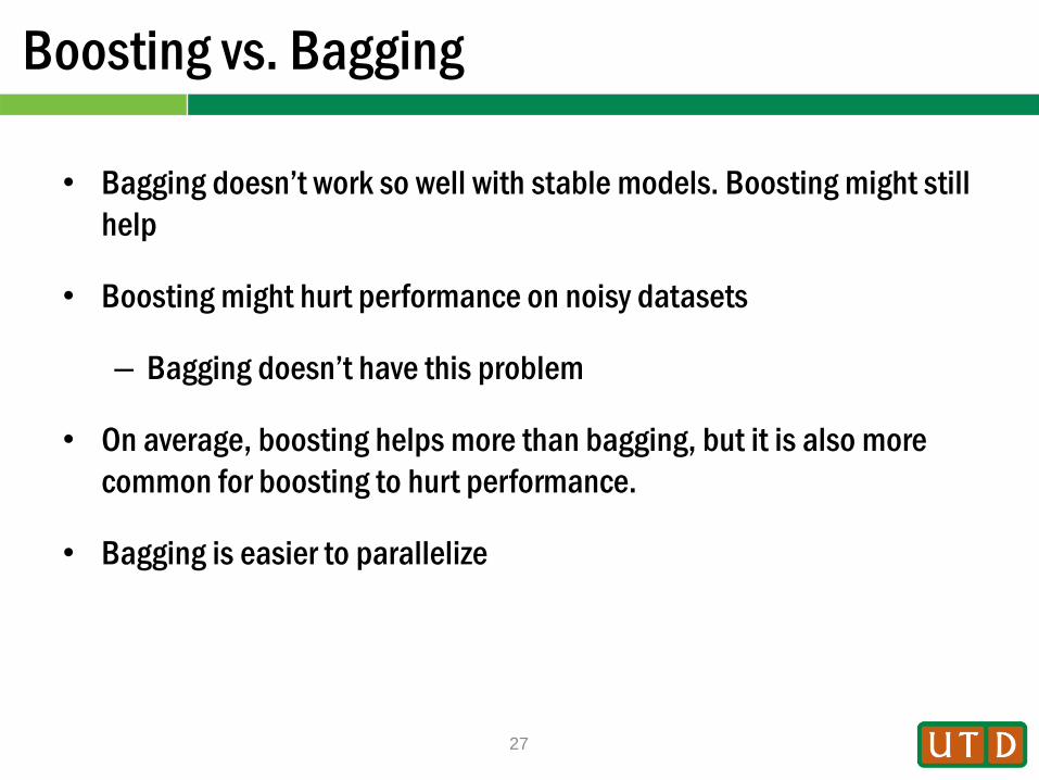
Boosting vs. Bagging

• Bagging doesn’t work so well with stable models. Boosting might still

help

• Boosting might hurt performance on noisy datasets

– Bagging doesn’t have this problem

• On average, boosting helps more than bagging, but it is also more

common for boosting to hurt performance.

• Bagging is easier to parallelize

Other Approaches

• Mixture of Experts (See Bishop, Chapter 14)

• Cascading Classifiers

• many others…