1

Ensemble Learning: An

Introduction

Adapted from Slides by Tan,

Steinbach, Kumar

2

General Idea

Original

Training data

....D

1D

2 Dt-1

Dt

D

Step 1:

Create Multiple

Data Sets

C1

C2

Ct -1

Ct

Step 2:

Build Multiple

Classifiers

C*

Step 3:

Combine

Classifiers

3

Why does it work?

• Suppose there are 25 base classifiers

– Each classifier has error rate, = 0.35

– Assume classifiers are independent

– Probability that the ensemble classifier makes

a wrong prediction:

25

13

25 06.0)1(25

i

ii

i

4

Examples of Ensemble Methods

• How to generate an ensemble of

classifiers?

– Bagging

– Boosting

5

Bagging

• Sampling with replacement

• Build classifier on each bootstrap sample

• Each sample has probability (1 – 1/n)n of

being selected as test data

• Training data = 1- (1 – 1/n)n of the original

data

Original Data 1 2 3 4 5 6 7 8 9 10

Bagging (Round 1) 7 8 10 8 2 5 10 10 5 9

Bagging (Round 2) 1 4 9 1 2 3 2 7 3 2

Bagging (Round 3) 1 8 5 10 5 5 9 6 3 7

Training DataData ID

6

6

The 0.632 bootstrap

• This method is also called the 0.632 bootstrap

– A particular training data has a probability of

1-1/n of not being picked

– Thus its probability of ending up in the test

data (not selected) is:

– This means the training data will contain

approximately 63.2% of the instances

368.01

1 1

e

n

n

7

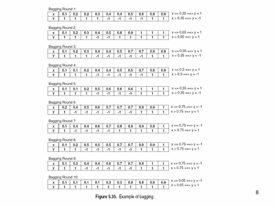
Example of Bagging

0.3 0.8 x

+1+1

-1

Assume that the training data is:

0.4 to 0.7:

Goal: find a collection of 10 simple thresholding classifiers that

collectively can classify correctly.

-Each simple (or weak) classifier is:

(x<=K class = +1 or -1 depending on

which value yields the lowest error; where K

is determined by entropy minimization)

8

9

Bagging (applied to training data)

Accuracy of ensemble classifier: 100%

10

Bagging- Summary

• Works well if the base classifiers are unstable (complement each other)

• Increased accuracy because it reduces the variance of the individual classifier

• Does not focus on any particular instance of the training data– Therefore, less susceptible to model over-

fitting when applied to noisy data

• What if we want to focus on a particular instances of training data?

11

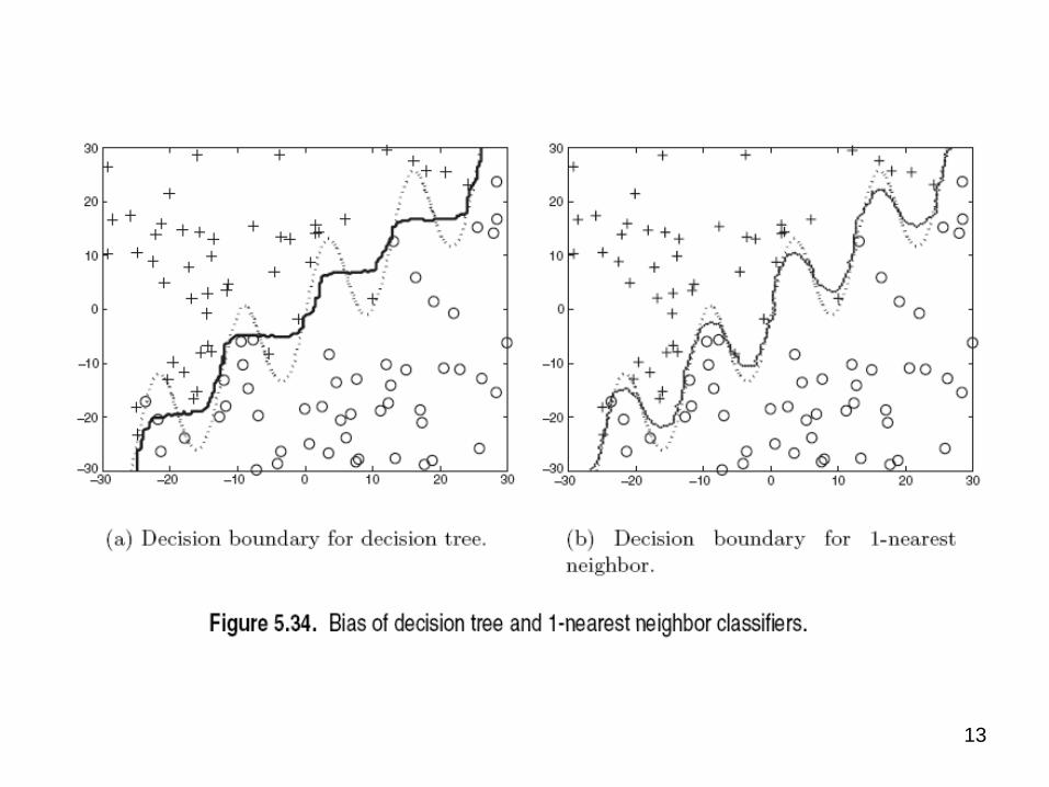
In general,

- Bias is contributed to by the training error; a complex

model has low bias.

-Variance is caused by future error; a complex model has

High variance.

- Bagging reduces the variance in the base classifiers.

12

13

14

Boosting

• An iterative procedure to adaptively

change distribution of training data by

focusing more on previously misclassified

records

– Initially, all N records are assigned equal

weights

– Unlike bagging, weights may change at the

end of a boosting round

15

Boosting

• Records that are wrongly classified will

have their weights increased

• Records that are classified correctly will

have their weights decreasedOriginal Data 1 2 3 4 5 6 7 8 9 10

Boosting (Round 1) 7 3 2 8 7 9 4 10 6 3

Boosting (Round 2) 5 4 9 4 2 5 1 7 4 2

Boosting (Round 3) 4 4 8 10 4 5 4 6 3 4

• Example 4 is hard to classify

• Its weight is increased, therefore it is more likely to be chosen again in subsequent rounds

16

Boosting

• Equal weights are assigned to each training instance (1/d for round 1) at first

• After a classifier Ci is learned, the weights are adjusted to allow the subsequent classifier

Ci+1 to “pay more attention” to data that were misclassified by Ci.

• Final boosted classifier C* combines the votes of each individual classifier– Weight of each classifier’s vote is a function of its

accuracy

• Adaboost – popular boosting algorithm

17

Adaboost (Adaptive Boost)

• Input:

– Training set D containing N instances

– T rounds

– A classification learning scheme

• Output:

– A composite model

18

Adaboost: Training Phase

• Training data D contain N labeled data (X1,y1), (X2,y2 ), (X3,y3),….(XN,yN)

• Initially assign equal weight 1/d to each data

• To generate T base classifiers, we need Trounds or iterations

• Round i, data from D are sampled with replacement , to form Di (size N)

• Each data’s chance of being selected in the next rounds depends on its weight– Each time the new sample is generated directly from

the training data D with different sampling probability according to the weights; these weights are not zero

19

Adaboost: Training Phase

• Base classifier Ci, is derived from training

data of Di

• Error of Ci is tested using Di

• Weights of training data are adjusted

depending on how they were classified

– Correctly classified: Decrease weight

– Incorrectly classified: Increase weight

• Weight of a data indicates how hard it is to

classify it (directly proportional)

20

Adaboost: Testing Phase

• The lower a classifier error rate, the more accurate it is,

and therefore, the higher its weight for voting should be

• Weight of a classifier Ci’s vote is

• Testing:

– For each class c, sum the weights of each classifier that

assigned class c to X (unseen data)

– The class with the highest sum is the WINNER!

i

ii

1ln

2

1

T

i

testiiy

test yxCxC1

)(maxarg)(*

21

Example: AdaBoost

• Base classifiers: C1, C2, …, CT

• Error rate: (i = index of

classifier, j=index of instance)

• Importance of a classifier:

N

j

jjiji yxCwN 1

)(1

i

ii

1ln

2

1

22

Example: AdaBoost

• Assume: N training data in D, T rounds, (xj,yj) are the training data, Ci, ai are the classifier and weight of the ith round, respectively.

• Weight update on all training data in D:

factorion normalizat theis where

)( ifexp

)( ifexp)(

)1(

i

jji

jji

i

i

ji

j

Z

yxC

yxC

Z

ww

i

i

T

i

testiiy

test yxCxC1

)(maxarg)(*

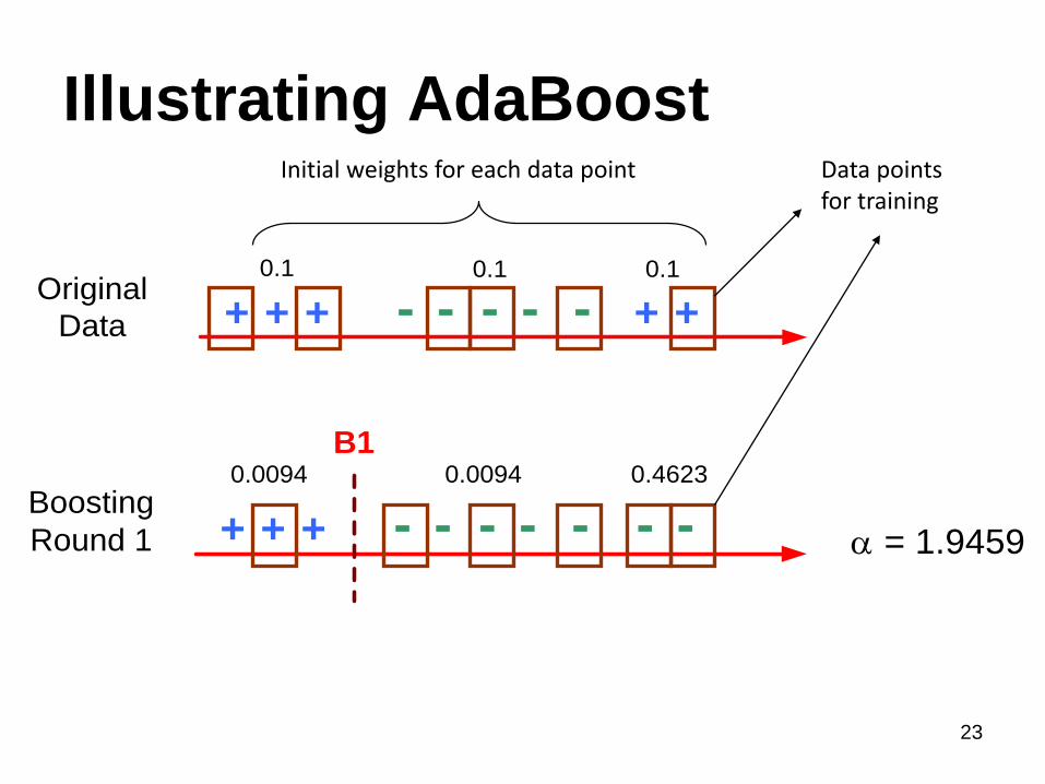
23

Boosting

Round 1 + + + -- - - - - -0.0094 0.0094 0.4623

B1

= 1.9459

Illustrating AdaBoostData points for training

Initial weights for each data point

Original

Data + + + -- - - - + +

0.1 0.1 0.1

24

Illustrating AdaBoost

Boosting

Round 1 + + + -- - - - - -

Boosting

Round 2 - - - -- - - - + +

Boosting

Round 3 + + + ++ + + + + +

Overall + + + -- - - - + +

0.0094 0.0094 0.4623

0.3037 0.0009 0.0422

0.0276 0.1819 0.0038

B1

B2

B3

= 1.9459

= 2.9323

= 3.8744

25

Random Forests

• Ensemble method specifically designed for

decision tree classifiers

• Random Forests grows many trees

– Ensemble of unpruned decision trees

– Each base classifier classifies a “new” vector of

attributes from the original data

– Final result on classifying a new instance: voting.

Forest chooses the classification result having the

most votes (over all the trees in the forest)

26

Random Forests

• Introduce two sources of randomness:

“Bagging” and “Random input vectors”

– Bagging method: each tree is grown using a

bootstrap sample of training data

– Random vector method: At each node, best

split is chosen from a random sample of m

attributes instead of all attributes

27

Random Forests

28

Methods for Growing the Trees

• Fix a m <= M. At each node– Method 1:

• Choose m attributes randomly, compute their information gains, and choose the attribute with the largest gain to split

– Method 2:• (When M is not very large): select L of the attributes

randomly. Compute a linear combination of the L attributes using weights generated from [-1,+1] randomly. That is, new A = Sum(Wi*Ai), i=1..L.

– Method 3: • Compute the information gain of all M attributes. Select the

top m attributes by information gain. Randomly select one of the m attributes as the splitting node.

29

Random Forest Algorithm:

method 1 in previous slide• M input features in training data, a number

m<<M is specified such that at each node, m features are selected at random out of the M and the best split on these m features is used to split the node. (In weather data, M=4, and m is between 1 and 4)

• m is held constant during the forest growing

• Each tree is grown to the largest extent possible (deep tree, overfit easily), and there is no pruning

30

Generalization Error of Random

Forests (page 291 of Tan book)

• It can be proven that the generalization Error <=

r(1-s2)/s2,

r is the average correlation among the trees

– s is the strength of the tree classifiers

• Strength is defined as how certain the classification results

are on the training data on average

• How certain is measured Pr(C1|X)-Pr(C2-X), where C1, C2

are class values of two highest probability in decreasing

order for input instance X.

• Thus, higher diversity and accuracy is good for

performance