Ensemble based updating of distributed, physically based, urban drainage models Morten Borup DTU Environment & Krüger A/S, Veolia VWS Denmark Morten Grum Krüger A/S, Veolia VWS Denmark Peter Steen Mikkelsen DTU Environment

Outline Urban drainage systems: Background

Physically based, distributed urban drainage models and what they can do

EnKF issues

Small example

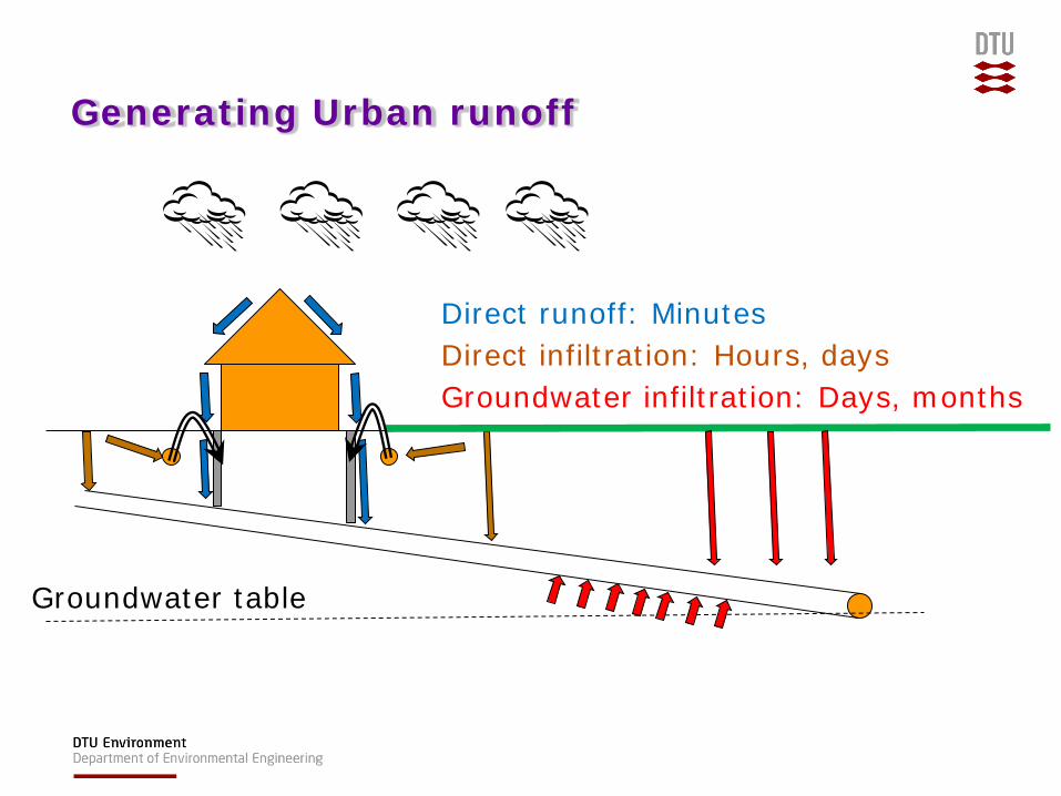
Direct infiltration: Hours, days

Generating Urban runoff

Direct runoff: Minutes

Groundwater table

Groundwater infiltration: Days, months

Urban drainage Systems

Urban drainage Systems

Urban drainage Systems

It’s a mess

Suboptimal for most events

Control is needed

Urban drainage Systems

Overflow structure

Differences to other hydrological system Fast response times

Closed conduits -> max. capacity

Overflows: Water disappears out of system

Real time control change hydraulic behaviour in seconds

Distributed, physically based, urban drainage models

Mixture of models: Runoff + Hydrodynamic + Water Quality

Developed mainly for design purposes

Can be build purely from physical data without calibration

Physically based models

Mike Urban model of Avedøre WWTP catchment

1707 sub-catchments 6601 Manholes 7749 Pipe sections 40 Pumps 40 Basins Etc.

5 km

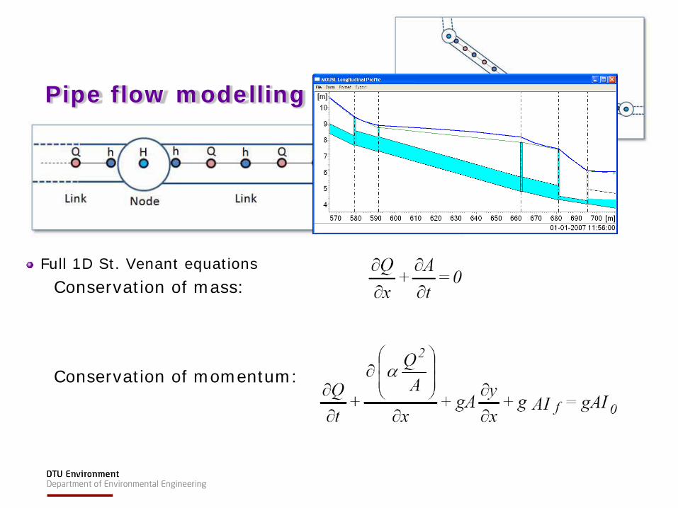
Full 1D St. Venant equations Conservation of mass: Conservation of momentum:

Pipe flow modelling

Multi purpose model Dimensioning of new system elements

Max frequency of water on terrain, basements etc.

Calculate yearly overflow and pollution loads

Documentation to authorities

Develop and optimize control strategies

Both PID and model predictive control using simple models

Are NOT used as online models

Purpose of online model

Warning

systems

Photo: Bente Schou

København

Lyngbyvej

16 aug. 2010

Real time health risk assesment

Error detection!

Model assisted real time control Aim:

reduce flooding reduce or redirect overflow Reduce cost of electricity consumption

Currently not used online because Computational cost – hardly run real time

Very uncertain rain input

No efficient update algorithm

Ensemble based updating

Dominating error source: Rain estimates Gauge:

Accurate in small area -> huge ensemble required to represent spatial variability

Radar Very inaccurate short term rain depth But spatial information -> reduced ensemble size

Q Update

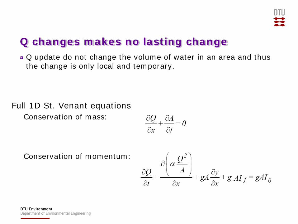
Q changes makes no lasting change Q update do not change the volume of water in an area and thus the change is only local and temporary.

Full 1D St. Venant equations Conservation of mass: Conservation of momentum:

H update

Overestimated observation variance Change in volume per change in h is depth dependent.

-> avoid perturbated observations

EnKF Example using

constructed radar data

Radar data

Typical Z-R relations i DK

0.1

1

10

100

100 1000 10000 100000Reflectivity Z

Rai

n in

tens

ity R

Light rain

Widespread

Showers

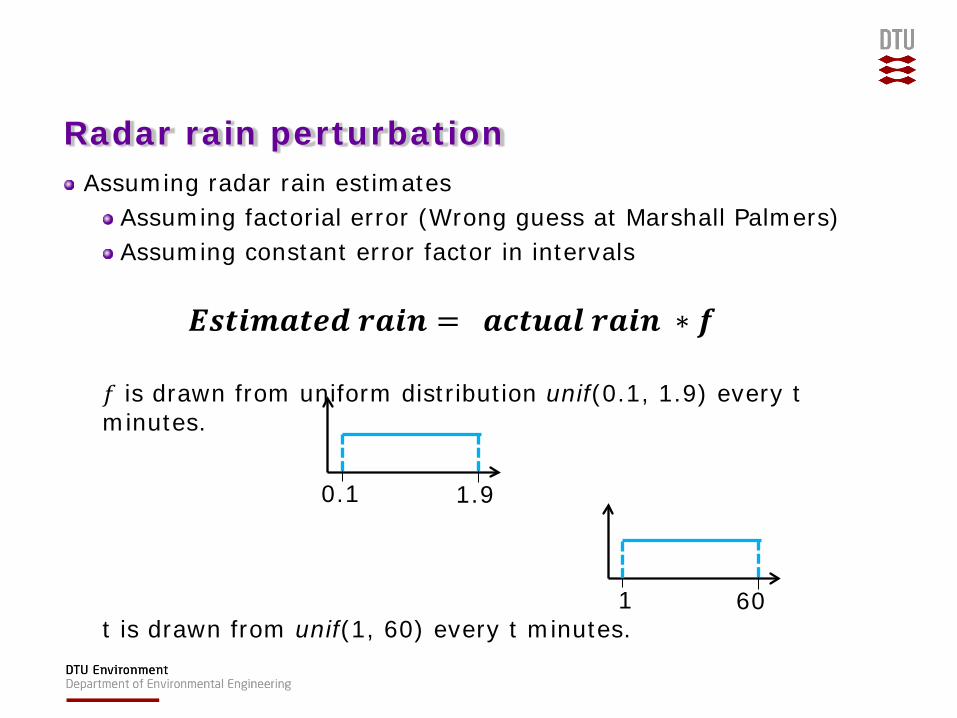
Assuming radar rain estimates Assuming factorial error (Wrong guess at Marshall Palmers) Assuming constant error factor in intervals

𝑬𝑬𝑬𝑬𝑬𝑬𝑬𝑬𝑬 𝒓𝑬𝑬𝒓 = 𝑬𝒂𝑬𝒂𝑬𝒂 𝒓𝑬𝑬𝒓 ∗ 𝒇 𝑓 is drawn from uniform distribution unif(0.1, 1.9) every t minutes. t is drawn from unif(1, 60) every t minutes.

Radar rain perturbation

0.1 1.9

1 60

Realization of f

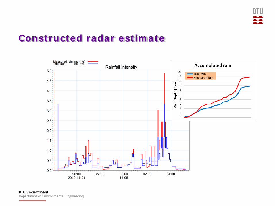
Constructed radar estimate

Model setup: Link and weir

A =57 ha

Tc = 60 min

Weir Point at Link 7

Situation without update

20:00 22:00 00:00 02:00 04:00 06:00

12.4

12.6

12.8

13

13.2

13.4

13.6

time

Wat

er L

evel

[m]

Water level at link 7

TruthBase

20:00 22:00 00:00 02:00 04:00 06:00 07:007.5

8

8.5

9

9.5

10

10.5

11

11.5

12

time

Wat

er L

evel

[m]

Water level at weir

TruthBase

Weir Link 7

Situation without update

20:00 22:00 00:00 02:00 04:00 06:00

12.4

12.6

12.8

13

13.2

13.4

13.6

time

Wat

er L

evel

[m]

Water level at link 7

TruthBase

20:00 22:00 00:00 02:00 04:00 06:00 07:007.5

8

8.5

9

9.5

10

10.5

11

11.5

12

time

Wat

er L

evel

[m]

Water level at weir

TruthBase

Ensemble of 20 – No update Weir Link 7

When updating using EnKF

3:00 4:00 5:0012

12.2

12.4

12.6

12.8

13

13.2

13.4

13.6

time

Wat

er L

evel

[m]

WL at Link7 chainage 935 - 5/11 2010

BaseTruthUpdated

Weir Link 7

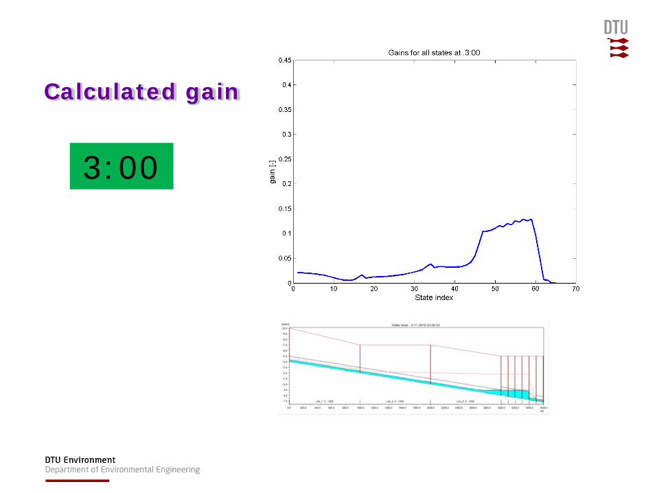
Gain and backwater

0 10 20 30 40 50 60 700

0.05

0.1

0.15

0.2

0.25

0.3

0.35

0.4

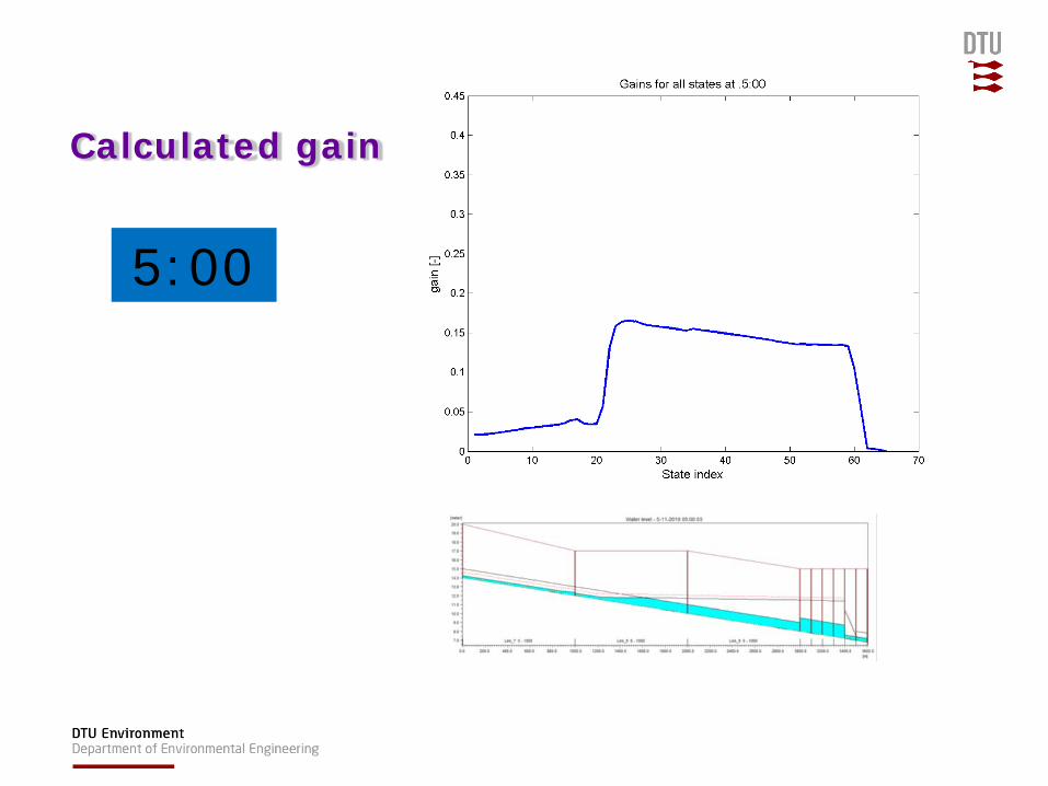
0.45Gains for all states at different times

State index

gain

[-]

0:001:002:003:004:005:006:00

Calculated gain

0:00

Calculated gain

1:00

Calculated gain

2:00

Calculated gain

3:00

Calculated gain

4:00

Calculated gain

5:00

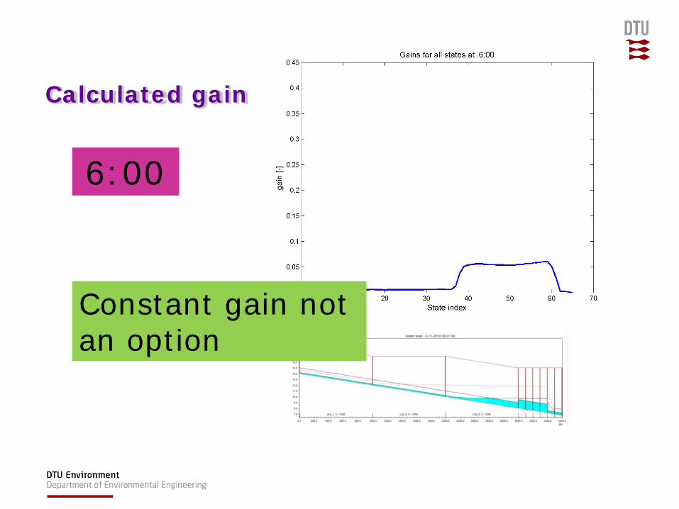
Calculated gain

6:00

Constant gain not an option

Non measurements

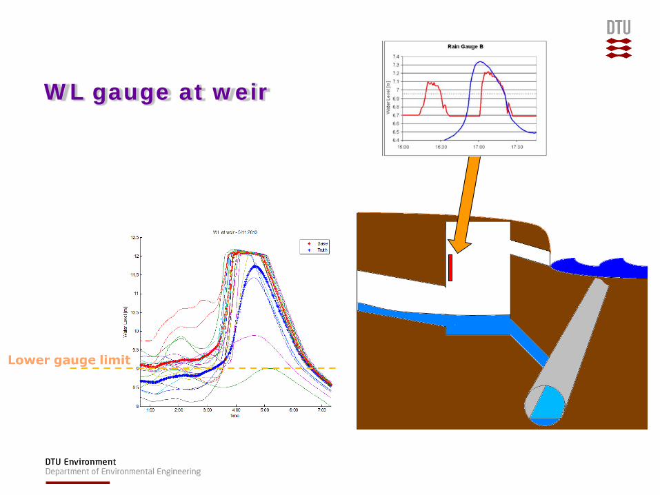
WL gauge at weir

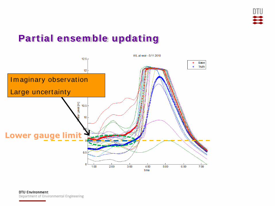
Partial ensemble updating

Imaginary observation

Large uncertainty

Partial DEnKF when no data Modified from [Sakov, 2008]1): d𝑦 = 𝑔𝑔𝑔𝑔𝑔𝑔𝑔𝑔𝑔𝑔 − 𝐻𝑥𝑓

𝑥𝑓 = 𝑔𝑔𝑔𝑚 𝑋𝑓

𝐴𝑓 = 𝑋𝑓 − [𝑥𝑓, . , . , . , 𝑥𝑓]

𝐴𝑎 = 𝐴𝑓 − 12𝐾𝐻𝐴

𝑓𝐵 B = Diagonal matrix. 1 where HAi>= dy, otherwise 0

𝑋𝑎 = 𝐴𝑎 + 𝑥𝑓, . , . , . , 𝑥𝑓

𝑥𝑎 = 𝑔𝑔𝑚𝑔𝑔𝑚(𝑋𝑎)

1) Sakov, P., & Oke, P. R. (2008). A deterministic formulation of the ensemble Kalman filter: an alternative to ensemble square root filters. Tellus A, 60(2), 361–371.

Partial DEnKF when no data Example

Summary Static gain not sufficient

Radar data is almost a requirement for EnKF

Ensemble spread can be reduced in periods without measurement

Probably best to avoid perturbed observations

Questions ?