Many of today’s liquid-liquid-extraction columns havelonger plant tenures thanthe engineers who are re-sponsible for pushing their

buttons. Over time, process engineerscome and go, while the original proce-dures and understanding of the columndesign become diluted. The upside tothis state of affairs is the implicationthat most columns could be runningbetter. The temptation that must beavoided, however, is jumping right intooptimization without first understand-ing what is going on inside the column.

For an effective step-by-step perfor-mance improvement strategy, see SixSteps to Better Liquid-Liquid Extrac-tion (box, right). As demonstrated bythese steps, it is important to revisitthe design basis when looking formeans of improvement.

THE FUNDAMENTALS OF EXTRACTIONLiquid-liquid extraction is a masstransfer operation whereby a feed solu-tion is contacted with a liquid solventthat is immiscible with one or more, butnot all, of the components of the solu-tion. During this contact, the materialto be removed from the feed (the solute)is transferred from the feed phase tothe solvent phase. The phases are thenseparated, generating an extract phase(solvent that has “picked up” the solute)and raffinate phase (original feed solu-tion minus the solute).

The concept of a column-type con-tactor is to allow the phases to flowcountercurrently due to the densitydifference between the liquids (Figure1). A well-designed extraction columnworks by generating a number of the-oretical stages within the column tomore efficiently transfer the solute

from one liquid phase to the other.Essential to understanding the per-

formance of an extraction column is theliquid-liquid equilibrium (LLE) dataset. These data can be shown in tabularformat, such as distribution coefficientversus solute concentration (see Table1 for an example), or in graphical for-mat, using an LLE curve, such as thatshown in Figure 2. Note that in extrac-tion, all concentrations are defined on asolute-free basis, which simplifies cal-culation and achieves straighter equi-librium and operating lines.

An LLE curve basically indicatesthe steady-state partitioning behaviorof the solute between the two phases.The y-axis is the concentration ofsolute in the extract (solvent) phase,and the x-axis is the concentration ofthe solute in the raffinate (feed) phase.

Every point on the curve also definesthe local distribution coefficient m:

m = ya / xa (1)

where a is the solute, ya is the concen-tration of component a in the extractliquid and xa is the concentration ofcomponent a in the raffinate liquid.

When the LLE data set is available,and a complete column material bal-ance is known, one can determine thenumber of theoretical stages that arenecessary to achieve a specified sepa-ration. One method is via graphicalsolution, whereby the LLE curve andoperating line are plotted on the samegraph, and the number of stagesstepped off using the standard Mc-Cabe-Thiele method that is commonlyassociated with distillation [1].

The McCabe-Thiele method is

Cover Story

44 CHEMICAL ENGINEERING WWW.CHE.COM NOVEMBER 2004

EnrichingLiquid-Liquid Extraction

A step-by-step guide to evaluating andimproving column efficiency

SIX STEPS TO BETTER LIQUID-LIQUID EXTRACTIONThe best way to improve liquid-liquid extraction performance is to first evaluate the col-umn and process materials. Then optimization can begin.

Evaluation steps:1. Find in the literature or generate the LLE data for the current process streams2. Obtain a complete material balance around the column, including flowrates and

solute concentrations for the feed, solvent, extract and raffinate3. Use either graphical solution, computer simulation, or the Kremser equation (see main

text) to calculate the current number of theoretical stages

Optimization steps:4. Evaluate how changes in the process variables will affect column performance to de-

termine options for optimization5. Depending on the results obtained in Step 4, perform pilot testing as necessary6. Based upon the results from Steps 4 and 5, modify equipment and/or process

Donald Glatz and Wendy ParkerKoch Modular Process Systems

TABLE 1. LIQUID-LIQUID EQUILIBRIUM DATA — MIBK, “A” AND WATERShake # %A in feed %A in raffinate %A in extract Dist. coeff. (m)1 0.43 0.14 0.14 1.002 3.36 3.33 3.62 1.093 6.73 6.98 6.95 1.004 10.08 9.73 11.32 1.165 13.44 13.07 13.76 1.05Average 1.06

44-48 CE 11/04 11/4/04 6:55 PM Page 44

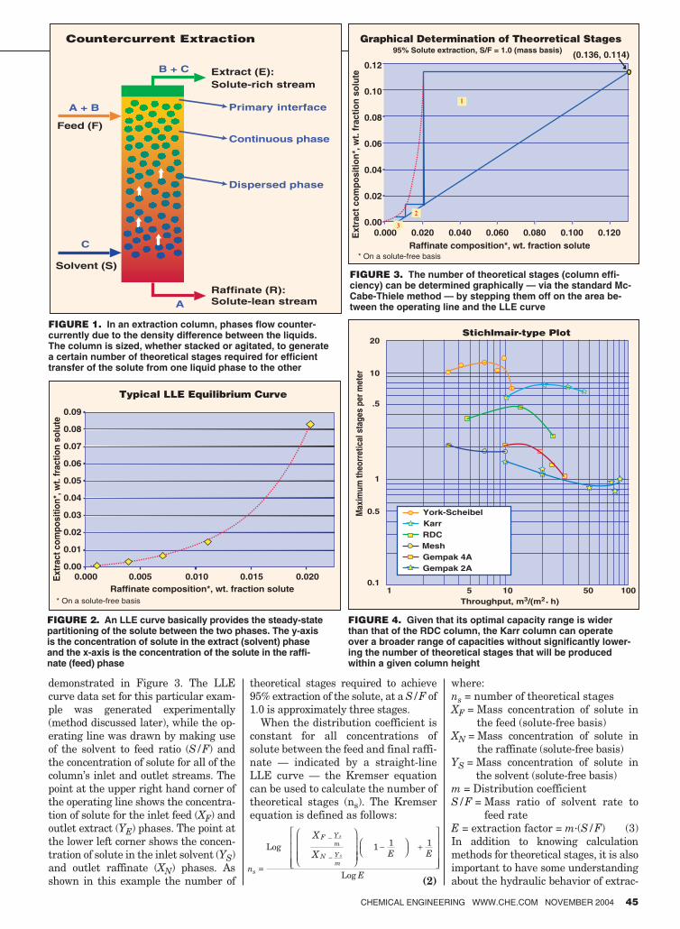
demonstrated in Figure 3. The LLEcurve data set for this particular exam-ple was generated experimentally(method discussed later), while the op-erating line was drawn by making useof the solvent to feed ratio (S/F) andthe concentration of solute for all of thecolumn’s inlet and outlet streams. Thepoint at the upper right hand corner ofthe operating line shows the concentra-tion of solute for the inlet feed (XF) andoutlet extract (YE) phases. The point atthe lower left corner shows the concen-tration of solute in the inlet solvent (YS)and outlet raffinate (XN) phases. Asshown in this example the number of

theoretical stages required to achieve95% extraction of the solute, at a S/F of1.0 is approximately three stages.

When the distribution coefficient isconstant for all concentrations ofsolute between the feed and final raffi-nate — indicated by a straight-lineLLE curve — the Kremser equationcan be used to calculate the number oftheoretical stages (ns). The Kremserequation is defined as follows:

(2)

where:ns = number of theoretical stagesXF = Mass concentration of solute in

the feed (solute-free basis) XN = Mass concentration of solute in

the raffinate (solute-free basis) YS = Mass concentration of solute in

the solvent (solute-free basis) m = Distribution coefficientS/F = Mass ratio of solvent rate to

feed rateE = extraction factor = m·(S/F) (3)In addition to knowing calculationmethods for theoretical stages, it is alsoimportant to have some understandingabout the hydraulic behavior of extrac-

CHEMICAL ENGINEERING WWW.CHE.COM NOVEMBER 2004 45

B + C

A

C

A + B

Feed (F)

Countercurrent Extraction

Solvent (S)

Extract (E):Solute-rich stream

Raffinate (R):Solute-lean stream

Primary interface

Continuous phase

Dispersed phase

FIGURE 1. In an extraction column, phases flow counter-currently due to the density difference between the liquids.The column is sized, whether stacked or agitated, to generatea certain number of theoretical stages required for efficienttransfer of the solute from one liquid phase to the other

Ext

ract

com

posi

tion*

, wt.

frac

tion

solu

te

Raffinate composition*, wt. fraction solute* On a solute-free basis

Typical LLE Equilibrium Curve

0.0000.00

0.01

0.02

0.03

0.04

0.05

0.06

0.07

0.08

0.09

0.005 0.010 0.015 0.020

Graphical Determination of Theorretical Stages

0.000 0.020 0.040 0.060 0.080 0.100

(0.136, 0.114)

0.1200.00

0.02

0.04

0.06

0.08

0.10

0.12

Raffinate composition*, wt. fraction solute* On a solute-free basis

95% Solute extraction, S/F = 1.0 (mass basis)

Ext

ract

com

posi

tion*

, wt.

frac

tion

solu

te

FIGURE 2. An LLE curve basically provides the steady-statepartitioning of the solute between the two phases. The y-axisis the concentration of solute in the extract (solvent) phaseand the x-axis is the concentration of the solute in the raffi-nate (feed) phase

Stichlmair-type Plot20

10

.5

1

1 5 10 50 100

0.5

0.1

Throughput, m3/(m2• h)

Max

imum

theo

rret

ical

sta

ges

per m

eter

Gempak 2AGempak 4AMeshRDCKarrYork-Scheibel

FIGURE 3. The number of theoretical stages (column effi-ciency) can be determined graphically — via the standard Mc-Cabe-Thiele method — by stepping them off on the area be-tween the operating line and the LLE curve

FIGURE 4. Given that its optimal capacity range is widerthan that of the RDC column, the Karr column can operateover a broader range of capacities without significantly lower-ing the number of theoretical stages that will be producedwithin a given column height

44-48 CE 11/04 11/4/04 6:55 PM Page 45

tion columns and how it can affect effi-ciency. For example, efficiency curvesfor several agitated extraction columnsare shown in Figure 4 [2]. The curvesshow how the column efficiency (onthese curves, theoretical stages per unitheight) changes with throughput (sumof the flowrates of both phases, dividedby column cross-sectional area).

Looking at the curve for the RDC (ro-tating disc column) reveals that the effi-ciency initially increases steadily for in-creasing capacity, then reaches amaximum, and finally begins to fall offsteadily after this point. Thus, if the col-umn is not operating near the optimalcapacity point, a significantly lowernumber of theoretical stages will beproduced within a given column height.The curve for the Karr Column on theother hand, is much flatter over a broadrange of capacities. Thus, it can operatewith peak efficiency over a wider rangeof capacities than the RDC.

EVALUATION STEPSThe first steps of extraction columnoptimization are generally evaluationsteps. For illustration of them, con-sider a performance evaluation for aKarr column that had been operatingfor over 20 years. The column wasused to extract a product — desig-nated here as “A” — from an aqueous

feed stream using methyl isobutyl ke-tone (MIBK) as the solvent.

The production column was operat-ing at a throughput of 1,200 (gal/h)/ft2

and a S/F of 1.24. Typical feed con-tained 14.2% A and the average raffi-nate concentration was 0.26% A. Therewere three objectives of the evaluation:1. Understand the performance in the

existing production column2. Evaluate changes in the process

variables that will reduce XN from0.26% to 0.1%

3. Determine the effects of increasingthe capacity by 50%

Step 1. Generate LLE dataThese data are generated via a proce-dure known as a “shake test” that es-tablishes a perfect equilibrium stage.Figure 5 shows one type of equipmentoften used to perform these tests. This1,000–2,000-ml reactor type flask(glass) is jacketed for temperature con-trol and outfitted with a standard labo-ratory type agitator having a half-moonimpeller. Feed solutions with varyingsolute concentrations are added to theflask along with the desired amount ofsolvent (depending on the S/F).

The two-phase mixture is allowed toheat up to the desired temperatureand then the phases are mixed vigor-ously for the length of time needed to

reach steadystate (generally about 2minutes for most applications). Thephases are then allowed to separate,and both phases are subsequently ana-lyzed to determine the solute concen-tration. A total of five to six feed sam-ples are tested with solute contentranging between those of the feed con-centration and the desired raffinateconcentration. The analytical resultsfrom each pair of samples are thenused to calculate the distribution coef-ficient for each shake test.

If the results show a relatively con-stant distribution coefficient, then theKremser equation can be used for the-oretical stage calculations. If, however,the distribution coefficient changessignificantly with concentration, thenthe graphical solution method or com-puter simulation must be used. For thecurrent example, the equilibrium dataare shown in Table 1.

Step 2. Material balanceThe equations for the material balance(on a solute-free basis) are as follows:

(4)

(5)

Cover Story

46 CHEMICAL ENGINEERING WWW.CHE.COM NOVEMBER 2004

Variable-speed drive

ThermometerBaffle

Temperingwater in

Drain

Temperingwater out

Bench-Scale Test Apparatus

A*+B*

FeedA+B

C

BA*+C*

A+CB*

BA*+C*

AC*

CB*

CA*+B*Solvent

Extraction Raffinatestripping

* These compounds are present in relatively small quantities

Solventrecovery

Extract

Raffinate

Typical Extraction System

FIGURE 5. This 1,000–2,000-ml reactor-type flask(glass) is jacketed for temperature control and fitted witha standard laboratory type agitator and half-moon im-peller. A total of five to six feed samples, with a solutecontent ranging between the feed concentration and thedesired raffinate concentration, are tested. The analyticalresults from each pair of samples are then used to calcu-late the distribution coefficient for each shake test

FIGURE 6. After leaving the extraction column, the two prod-uct streams are distilled to generate a purified Product Astream and an MIBK overhead stream that is recycled back tothe extraction column. Thus, in this case the concentration ofsolute (A) in the solvent is not zero, but 0.07%

44-48 CE 11/04 11/4/04 6:56 PM Page 46

(6)

S = Mass solvent rate � (7)(1–solute concentration in the solvent)

F = Mass feed rate � (8)(1–solute concentration in the solvent)

The plant operating conditions for theexample system are summarized inTable 2. The distribution coefficient isin the range of 0.99 to 1.16, which iscertainly close enough to be consid-ered constant. Therefore, the averagevalue of 1.06 can be used with theKremser equation to accurately de-scribe the extraction process.

It should be noted that the concen-tration of solute (A) in the solvent is notzero, but 0.07%. This is because theMIBK-extract phase, after leaving theextraction column, is distilled to gener-ate a purified Product A stream and anMIBK overhead stream that is recycledback to the extraction column (Figure6). The design and operation of this dis-tillation column will determine theamount of solute in the recycle solventstream. In many cases, the amount ofsolute in the recycle solvent will have asignificant impact on the performanceof the extraction column. Thus, this as-pect should not be overlooked when at-tempting to improve the performanceof the extraction column.

Step 3. Assess the current number of theoretical stagesOnce the column performance dataand the distribution coefficient of 1.06are plugged into the Kremser equa-tion, the number of theoretical stagesare calculated to be 10.7 stages.

(2a)ns = 10.7 stages

OPTIMIZATION STEPS Step 4. Determine the options for optimizationAt this point it is time to use theknown column performance and theKremser equation to evaluate the ef-fect of changes to the key processvariables. By changing individualinput variables, one can quickly cal-culate the effect on the column per-formance. (Keep in mind that the cur-rent column height is fixed.) This hasbeen done as shown in Table 3 (whichassumes any consistent mass unitsfor S and F) and outlined below:Run 1. Current performance. Thisrun shows the current performance ofthe extraction column. With 10.7 the-oretical stages and S/F = 1.24, theraffinate concentration, XN, is 0.26%.Run 2. Calculate the number ofstages required to achieve 0.1% A inraffinate with 0.07% A in solvent.Here we see that for the same operatingconditions, 17.0 theoretical stages arerequired to achieve 0.1% raffinate con-centration. There are three ways to pro-vide more theoretical stages; (1) In-creasing the existing column height by60%, (2) changing to a more-efficientcolumn design, or (3) increasing the ef-ficiency in the existing column.

Obviously, the first two options willinvolve equipment modifications andsignificant capital spending. Also, it isdoubtful that a more efficient columnthan the Karr column can be utilizedfor this process. The third option willgenerally require either EVOP (evolu-tionary optimization) testing in the pro-duction column, or a pilot-plant testingin a scaled-down version of this column.The benefit of increased product recov-ery (and possible reduced effluent treat-ment cost) for all options would need tobe weighed against the cost of the test-ing and/or capital expenditures.Run 3. Calculate potential effects(on number of stages required to

achieve 0.1% A in raffinate) ofusing pure solvent. This rundemonstrates that in the existing col-umn, if pure solvent were used (nosolute in the solvent), then an in-crease to 13.1 theoretical stageswould be required. Therefore, even iffresh solvent were used, the existingcolumn could not generate 0.1% raffi-nate concentration unless the stageefficiency was also improved or morestages were added to the column.Run 4. Calculate XN for currenttheoretical stages and 0.02% A insolvent. This run shows that decreas-ing the solute in the recycle solventfrom 0.07% to 0.02% (with no otherchanges) will result in a decrease inthe raffinate concentration from0.26% to 0.21%. Thus, based upon thecalculations for Runs 3 and 4, the ef-fect of the solute in the recycle solventhas only a minor impact on the finalraffinate concentration.Run 5. Calculate S/F required toachieve 0.1% A in raffinate forcurrent theoretical stages. This runshows that increasing the solvent-to-feed ratio from 1.24 to 1.51 will pro-duce the required raffinate concentra-tion of 0.1%. This is obviously theeasiest solution for improving the re-covery of product A. However, thevalue of the increased product recov-ery must also be evaluated against theincreased operating cost required todistill and recycle 22% more MIBK. Inaddition, the downstream distillationequipment and the extractor musthave enough excess capacity for thisoption to be viable.Run 6. Calculate A in raffinate for1,800 (gal/h)/ft2, 0.07% A in solventand S/F = 1.24. Early process devel-opment reports were found that docu-mented the initial pilot-plant testingin a 1-in. dia. Karr column. This dataset indicated that when the through-put of the column was increased by

CHEMICAL ENGINEERING WWW.CHE.COM NOVEMBER 2004 47

TABLE 2. EXAMPLE OPERATINGCONDITIONS

Stream Concentration of “A”

Feed (XF) 14.2%

Raffinate (XN) 0.26%

Solvent (YS) 0.07%

S/F 1.24

TABLE 3. “A” EXTRACTION WITH MIBK IN 24-IN.-DIA. KARR COLUMNRun XF XN YS S F m E ns1 0.142 0.0026 0.0007 1.24 1.00 1.06 1.31 10.72 0.142 0.0010 0.0007 1.24 1.00 1.06 1.31 17.03 0.142 0.0010 0.0000 1.24 1.00 1.06 1.31 13.14 0.142 0.0021 0.0002 1.24 1.00 1.06 1.31 10.85 0.142 0.0010 0.0007 1.51 1.00 1.06 1.61 10.76 0.142 0.0048 0.0007 1.24 1.00 1.06 1.31 8.0

44-48 CE 11/04 11/4/04 6:57 PM Page 47

50% (1,200 to 1,800 (gal/h)/ft2), thecolumn’s efficiency decreased by 25%.

Since the height of the current col-umn is effectively fixed, a lower effi-ciency would translate into a reductionin the number of theoretical stages(from 10.7 to 8.0) that are achieved in-side the column. As shown, the result-ing raffinate concentration (for S/F =1.24) is expected to increase to 0.48%.In short, the engineer has the option tooperate this column at higher capacity,but with the disadvantage of higherraffinate concentration as the columnapproaches 1,800 (gal/h)/ft2.

Step 5. Perform pilot testing as necessaryIf previous pilot data are not avail-able, then the authors recommendcaution when increasing the capacityin a production column. Flooding (in-ability to separate the phases) willeventually occur when the requiredthroughput is greater then the maxi-

mum that the column can process.Thus, it is usually best to performtests in a pilot-size column to deter-mine the systems limitations beforesignificantly increasing the capacityof an operating column.

Step 6. Modify equipment or process The action taken in this final stepwill depend on the options discoveredin Step 5 and their associated costs.And, even if the methods for improve-ment are infeasible for the shortterm, a better understanding of yourcolumn is valuable at any time. ■

Edited by Rebekkah Marshall

Cover Story

48 CHEMICAL ENGINEERING WWW.CHE.COM NOVEMBER 2004

adlinks.che.com/3648-48

AuthorDonald Glatz is manager ofextraction technology at KochModular Process Systems (45Eisenhower Drive, Paramus,NJ 07652; Phone: 201-368-2929; Fax: 201-368-8989;Email: donaldg@modular-process.com; Web: www.mod-ular-process.com). His activi-ties include evaluation andoptimization of liquid-liquid-extraction processes, and

scaleup and design of extraction columns. Hehas been working in this field for the past 15years. Prior experience includes 13 years inprocess development for GAF Chemical Corp.and General Foods Corp. Glatz holds a B.S.ChEfrom Rensselaer Polytechnic Institute and anM.B.A. from Fairleigh Dickenson University.

Wendy Parker works asmanager of pilot-plant techni-cal operations and as a seniorprocess engineer for KochModular Process Systems,LLC (Email: wendyp@modu-lar-process.com). Her activi-ties include pilot-scale devel-opment, as well as simulationand design of commercial dis-tillation and extractionprocesses. She has been

working with KMPS for the past nine years.Prior experience includes six years in processand plant engineering for Hoffmann-LaRocheand General Mills. Wendy holds a B.S.ChEfrom the University of Wisconsin-Madison.

References1. Cusack, R., Fremeaux, P., and Glatz, D., A

Fresh Look at Liquid-Liquid Extraction,Chem. Eng., February 1991, pp. 66–76.

2. Cusack, R., Holmes, T., Karr, A., The Otto H.York Co., paper delivered at AIChE SummerNational Meeting, August 17, 1987.

44-48 CE 11/04 11/5/04 12:14 PM Page 48