Enhancements to basic decision tree induction, C4.5.

Enhancements to basic decision tree induction, C4.5

Zur Anzeige wird der QuickTime™ Dekompressor „TIFF (LZW)“

benötigt.

This is a decision tree for credit risk assessment It classifies all examples of the table correctly


benötigt.

ID3 selects a property to test at the current node of the tree and uses this test to partition the set of examples

The algorithm then recursively constructs a sub tree for each partition

This continuous until all members of the partition are in the same class

• That class becomes a leaf node of the tree

The credit history loan table has following information p(risk is high)=6/14 p(risk is moderate)=3/14 p(risk is low)=5/14

€

I(credit _ table) = −6

14log2

6

14

⎛

⎝ ⎜

⎞

⎠ ⎟−

3

14log2

3

14

⎛

⎝ ⎜

⎞

⎠ ⎟−

5

14log2

5

14

⎛

⎝ ⎜

⎞

⎠ ⎟

I(credit _ table) =1.531 bits

gain(income)=I(credit_table)-E(income)

gain(income)=1.531-0.564

gain(income)=0.967 bits

gain(credit history)=0.266

gain(debt)=0.581

gain(collateral)=0.756

Overfiting Reduced-Error Pruning C4.5

From Trees to Rules Contigency table (statistics)

continous/unknown attributescross-validation

Overfiting The ID3 algorithm grows each branch of the

tree just deeply enough to perfectly classify the training examples

Difficulties may be present: When there is noise in the data When the number of training examples is too small to

produce a representative sample of the true target function

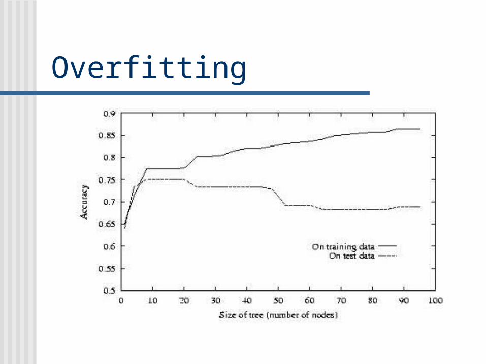
The ID3 algorithm can produce trees that overfit the training examples

We will say that a hypothesis overfits the training examples if some other hypothesis that fits the training examples less well actually performs better over the entire distribution of instances (included instances beyond training set)

Overfitting

Consider error of hypothesis h over Training data: errortrain(h)

Entire distribution D of data: errorD(h)

Hypothesis hH overfits training data if there is an alternative hypothesis h’H such that

errortrain(h) < errortrain(h’)

and

errorD(h) > errorD(h’)

Overfitting

How can it be possible for a tree h to fit the training examples better than h’

But to perform more poorly over subsequent examples

One way this can occur when the training examples contain random errors or noise

Training ExamplesDay Outlook Temp. Humidity Wind Play TennisD1 Sunny Hot High Weak NoD2 Sunny Hot High Strong NoD3 Overcast Hot High Weak YesD4 Rain Mild High Weak YesD5 Rain Cool Normal Weak YesD6 Rain Cool Normal Strong NoD7 Overcast Cool Normal Weak YesD8 Sunny Mild High Weak NoD9 Sunny Cold Normal Weak YesD10 Rain Mild Normal Strong YesD11 Sunny Mild Normal Strong YesD12 Overcast Mild High Strong YesD13 Overcast Hot Normal Weak YesD14 Rain Mild High Strong No

Decision Tree for PlayTennisOutlook

Sunny Overcast Rain

Humidity

High Normal

Wind

Strong Weak

No Yes

Yes

YesNo

Consider of adding the following positive training example, incorrectly labaled as negative

Outlook=Sunny, Temperature=Hot, Humidty=Normal, Wind=Strong, PlayTenis=No

The addition of this incorrect example will now cause ID3 to construct a more complex tree

Because the new example is labaled as a negative example, ID3 will search for further refinements to the tree

As long as the new errenous example differs in some attributes, ID3 will succeed in finding a tree

ID3 will output a decision tree (h) that is more complex then the orginal tree (h‘)

Given the new decision tree a simple consequence of fitting nosy training examples,h‘ will outpreform h on the test set

Avoid Overfitting

How can we avoid overfitting? Stop growing when data split not statistically

significant Grow full tree then post-prune

How to select ``best'' tree: Measure performance over training data Measure performance over separate validation

data set

Reduced-Error Pruning Split data into training and validation set Do until further pruning is harmful:

Evaluate impact on validation set of pruning each possible node (plus those below it)

Greedily remove the one that most improves the validation set accuracy

Produces smallest version of most accurate subtree

Effect of Reduced Error Pruning

Rule-Post Pruning Convert tree to equivalent set of rules Prune each rule independently of each other Sort final rules into a desired sequence to use

Method used in C4.5

Changes and additions to ID3 in C4.5 Includes a module called C4.5RULES, that can

generate a set of rules from any decision tree It uses pruning heuristic to simplify decision

trees in an attempt to produce results Easier to understand Less dependent on a particular training set used

The original test selection heuristic has also been changed

Converting a Tree to RulesOutlook

Sunny Overcast Rain

Humidity

High Normal

Wind

Strong Weak

No Yes

Yes

YesNo

R1: If (Outlook=Sunny) (Humidity=High) Then PlayTennis=No R2: If (Outlook=Sunny) (Humidity=Normal) Then PlayTennis=YesR3: If (Outlook=Overcast) Then PlayTennis=Yes R4: If (Outlook=Rain) (Wind=Strong) Then PlayTennis=NoR5: If (Outlook=Rain) (Wind=Weak) Then PlayTennis=Yes

It is not satisfactory to form a rule set by enumerating all paths of the tree...

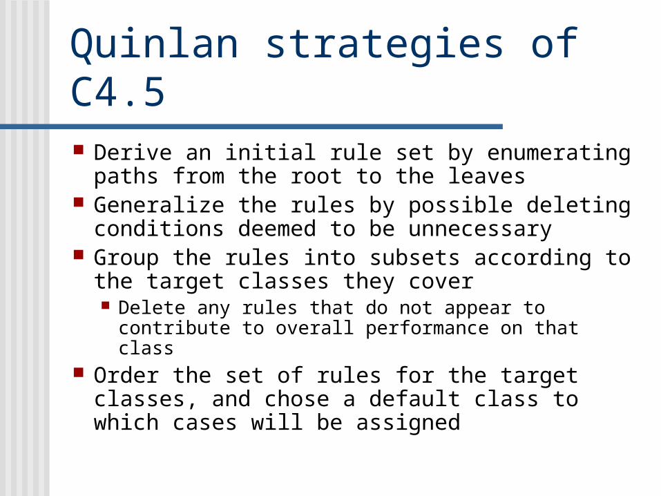
Quinlan strategies of C4.5 Derive an initial rule set by enumerating paths from

the root to the leaves Generalize the rules by possible deleting

conditions deemed to be unnecessary Group the rules into subsets according to the target

classes they cover Delete any rules that do not appear to contribute to

overall performance on that class Order the set of rules for the target classes, and

chose a default class to which cases will be assigned

The resultant set of rules will probably not have the same coverage as the decision tree

Its accuracy should be equivalent Rules are much easier to understand Rules can be tuned by hand by an expert

From Trees to Rules

Once an identification tree is constructed, it is a simple matter to concert it into a set of equivalent rules

• Example from Artificial Intelligence, P.H. Winston 1992


benötigt.

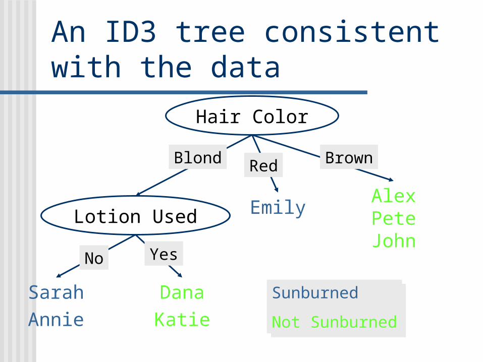
An ID3 tree consistent with the data

Hair Color

Lotion Used

Sarah

Annie

Dana

Katie

EmilyAlexPeteJohn

Blond Red Brown

No Yes

Sunburned

Not Sunburned

Sunburned

Not Sunburned

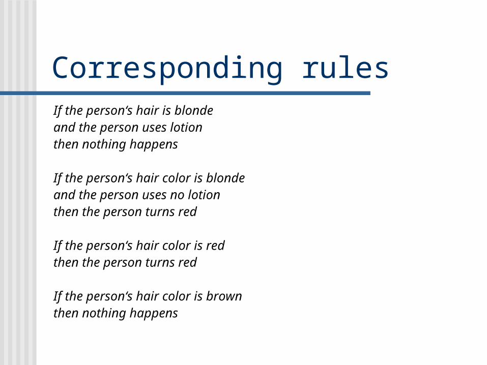
Corresponding rulesIf the person‘s hair is blonde and the person uses lotionthen nothing happens

If the person‘s hair color is blonde and the person uses no lotionthen the person turns red

If the person‘s hair color is redthen the person turns red

If the person‘s hair color is brownthen nothing happens

Unnecessary Rule Antecendents should be eliminated

If the person‘s hair is blonde and the person uses lotionthen nothing happens

Are both antecendents are really necessary? Dropping the first antecendent produce a rule with the same results

If the the person uses lotionthen nothing happens

To make such reasonning easier, it is often helpful to construct a contigency table

it shows the degree to which a result is contigent on a property

In the following contigency table one sees the number of lotion users who are blonde and not blonde and are sunburned or not

• Knowledge about whether a person is blonde has no bearing whether it gets sunburned

No change Sunburned

Person is blonde (uses lotion)

2 0

Person is not blonde (uses lotion)

1 0

Check for lotion for the same rule

Has a bearing on the result

No change Sunburned

Person uses lotion 2 0

Person uses no lotion 0 2

Unnecessary Rules should be EliminatedIf the person uses lotionthen nothing happens

If the person‘s hair color is blonde and the person uses no lotionthen the person turns red

If the person‘s hair color is redthen the person turns red


Note that two rules have consequent that indicate that a person will turn red, and two that indicate a person will turn red

One can replace either the two of them by a default rule

Default ruleIf the person uses lotionthen nothing happens


If no other rule appliesthen the person turns red

Contigency table(statistical theory)

R1 and R2 represent the Boolean states of an antecedent for the conclusions C1 and C2 (C2 is the negation of C1)

x11, x12, x21 and x22 represent the frequencies of each antecedent-consequent pair

R1T, R2T, CT1, CT2 are the marginal sums of the rows and columns, respectively

The marginal sums and T, the total frequency of the table, are used to calculate expected cell values of the test for independence


benötigt.

The general formula for obtaining the expected frequency of any cell

Select the test to be used to calculate, for highest expected frequency > 10 chi-square test, else Fisher‘s test

€

eij =RiTCTj

T

∑ −=

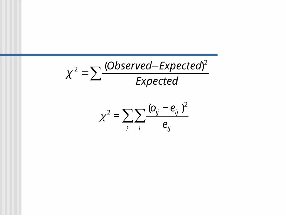
Expected

ExpectedObserved 22 )(

χ

€

χ 2 =(oij − eij )

2

eiji

∑i

∑

if the person's hair color is blond and the person uses no lotionthen the person turns red

Actual

Expected


benötigt.


benötigt.


benötigt.

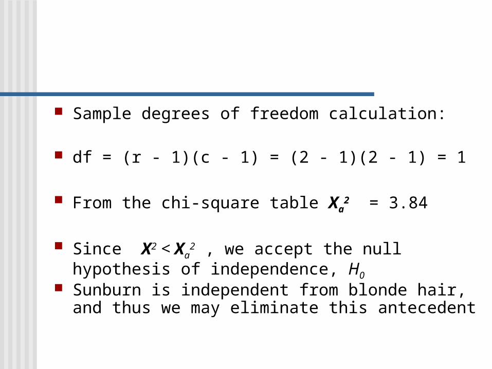
Sample degrees of freedom calculation:

df = (r - 1)(c - 1) = (2 - 1)(2 - 1) = 1

From the chi-square table Xa2 = 3.84

Since X2 < Xa2 , we accept the null hypothesis of

independence, H0

Sunburn is independent from blonde hair, and thus we may eliminate this antecedent

New test selection heuristic The original test selection heuristic based

on information gain proved unsatisfactory Favor attributes with a large number of

outcomes over attributes with a smaller number

Attributes that split the data into a large number of singelton classes (classifying patients in a medical database by their name) score well because I(Ci) is zero!

€

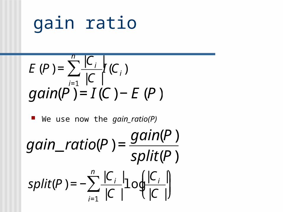
E(P) =| Ci |

| C |i=1

n

∑ I(Ci)

gain ratio

€

E(P) =| Ci |

| C |i=1

n

∑ I(Ci)

€

gain(P) = I(C) − E(P)

€

gain _ ratio(P) =gain(P)

split(P)

€

split(P) = −| Ci |

| C |i=1

n

∑ log| Ci |

| C |

⎛

⎝ ⎜

⎞

⎠ ⎟

We use now the gain_ratio(P)

Other Enhancements

Allow for continuous-valued attributes Dynamically define new discrete-valued attributes that partition

the continuous attribute value into a discrete set of intervals

Handle missing attribute values Assign the most common value of the attribute Assign probability to each of the possible values

Attribute construction Create new attributes based on existing ones that are sparsely

represented This reduces fragmentation, repetition, and replication

Continuous Valued AttributesCreate a discrete attribute to test continuous Temperature = 24.50C (Temperature > 20.00C) = {true, false}

Where to set the threshold?

Temperatur 150C 180C 190C 220

C240

C270

C

PlayTennis No No Yes Yes Yes No

(see paper by [Fayyad, Irani 1993]

Unknown Attribute Values

What is some examples missing values of an attribute A? Use training example anyway sort through tree If node n tests A, assign most common value of A among other

examples sorted to node n Assign most common value of A among other examples with same

target value

Assign probability pi to each possible value vi of A Assign fraction pi of example to each descendant in tree

Classify new examples in the same fashion

Attributes with Cost

Consider: Medical diagnosis : blood test costs 1000 SEK Robotics: width_from_one_feet has cost 23 secs.

How to learn a consistent tree with low expected cost?

Replace Gain by :

Gain2(A)/Cost(A) [Tan, Schimmer 1990]

2Gain(A)-1/(Cost(A)+1)w w [0,1] [Nunez 1988]

Other Attribute Selection Measures

Gini index (CART, IBM IntelligentMiner)

All attributes are assumed continuous-valued Assume there exist several possible split values for

each attribute May need other tools, such as clustering, to get the

possible split values Can be modified for categorical attributes

Cross-Validation

Estimate the accuracy of a hypothesis induced by a supervised learning algorithm

Predict the accuracy of a hypothesis over future unseen instances

Select the optimal hypothesis from a given set of alternative hypotheses Pruning decision trees Model selection Feature selection

Combining multiple classifiers (boosting)

Holdout Method

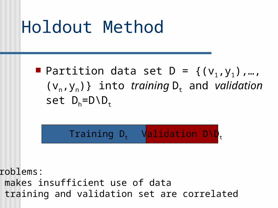
Partition data set D = {(v1,y1),…,(vn,yn)} into training Dt and validation set Dh=D\Dt

Training Dt Validation D\Dt

Problems: • makes insufficient use of data• training and validation set are correlated

Cross-Validation k-fold cross-validation splits the data set D into

k mutually exclusive subsets D1,D2,…,Dk

Train and test the learning algorithm k times, each time it is trained on D\Di and tested on Di

D1 D2 D3 D4

D1 D2 D3 D4 D1 D2 D3 D4

D1 D2 D3 D4 D1 D2 D3 D4

Cross-Validation Uses all the data for training and testing Complete k-fold cross-validation splits the

dataset of size m in all (m over m/k) possible ways (choosing m/k instances out of m)

Leave n-out cross-validation sets n instances aside for testing and uses the remaining ones for training (leave one-out is equivalent to n-fold cross-validation)

In stratified cross-validation, the folds are stratified so that they contain approximately the same proportion of labels as the original data set

Overfiting Reduced-Error Pruning C4.5

From Trees to Rules Contigency table (statistics)

continous/unknown attributescross-validation

Neural Networks Perceptron

Enhancements to basic decision tree induction, C4.5.

Documents

Transcript of Enhancements to basic decision tree induction, C4.5.