ORNL/TM-2000/26

ENGINEERING-ECONOMIC ANALYSES OF AUTOMOTIVE FUEL ECONOMY POTENTIAL

IN THE UNITED STATES

David L. Greene Center for Transportation Analysis

Oak Ridge National Laboratory

John DeCicco American Council for an Energy-Efficient Economy

January 2000

Prepared for the Office of Policy

U.S. Department of Energy Washington, DC

Prepared by the OAK RIDGE NATIONAL LABORATORY

Oak Ridge, Tennessee 37831-6073 Managed by

LOCKHEED MARTIN ENERGY RESEARCH CORP. for the

U. S. DEPARTMENT OF ENERGY under contract DE-AC05-96OR22464

iii

iv

TABLE OF CONTENTS

LIST OF FIGURES ....................................................................................................................v LIST OF TABLES......................................................................................................................v ACKNOWLEDGEMENTS.......................................................................................................vii ABSTRACT............................................................................................................................... ix 1. INTRODUCTION................................................................................................................. 1

2. METHODOLOGICAL ISSUES............................................................................................5 2.1 HOLDING OTHER ATTRIBUTES CONSTANT .........................................................7 2.2 TECHNOLOGY IMPACT ESTIMATES.......................................................................8 2.2.1 Market Readiness .................................................................................................8 2.2.2 Technology Interactions .......................................................................................9 2.2.3 Allocation of Technology Benefits......................................................................10 2.3 COSTS ...............................................................................................................12 2.4 UNCERTAINTY .........................................................................................................13 2.5 MARKET BEHAVIOR................................................................................................14 2.5.1 The Value of Fuel Savings, Risk and Information ...............................................14 3. LITERATURE REVIEW ....................................................................................................17 3.1 EARLY ASSESSMENTS: ENERGY CRISIS AND CAFE STANDARDS ................17 3.2 A SECOND OIL PRICE SHOCK AND CAFE RECONSIDERED..............................19 3.3 DEPARTMENT OF ENERGY (DOE) STUDIES........................................................23 3.4 ADVANCED TECHNOLOGIES.................................................................................25 3.5 ALTERNATIVE METHODS ......................................................................................27 4. REVIEW OF SIX RECENT STUDIES...............................................................................31 4.1 EEA STUDIES ............................................................................................................31 4.2 ACEEE STUDIES .......................................................................................................33 4.3 NATIONAL RESEARCH COUNCIL (1992) ..............................................................35 4.4 OFFICE OF TECHNOLOGY ASSESSMENT (1995) .................................................38 4.5 “5-LAB” STUDY (1997) .............................................................................................41 4.6 EIA “COSTS OF KYOTO” ANALYSIS (1998) ..........................................................44 5. DISCUSSION ...............................................................................................................47 5.1 COMPARISON OF COST CURVES...........................................................................47 5.2 IMPLIED FUEL PRICE ELASTICITIES ....................................................................49 5.3 SUGGESTIONS FOR FUTURE STUDY....................................................................52 6. CONCLUSIONS …………………………………………………………………………55 7. REFERENCES ...............................................................................................................57 APPENDIX ..........................................................................................................................65

v

vi

LIST OF FIGURES Figure 1. Trends in Fuel Economy Related Attributes of U.S. Light Duty Vehicles, 1975—1999..............................................................................................11 Figure 2. Net Value to Car Buyer of Fuel Economy Improvements from Fuel Economy Technologies.....................................................................................16 Figure 3. “Supply Curve” for Fuel Economy: Subcompact Cars, 1974.....................................18 Figure 4. Comparison of Early Technology Cost Curves .........................................................22 Figure 5. Passenger Car Fuel Economy Cost Curves Based on Six Studies ..............................48 Figure 6. Inferred Future Light Truck Fuel Economy Cost Curves from Three Studies............49 Figure 7. Fuel Economy Supply and Demand Curves for Passenger Cars.................................50 Figure 8. Fuel Economy Supply and Demand Curves for Light Trucks ....................................50

LIST OF TABLES Table 1. Fuel Economy Improvement of Technological and Design Changes, 1977 ................19 Table 2. Automobile MPG Levels and Costs Projected by the Office of Technology Assessment, 1982.....................................................................................................21 Table 3. TCSM Projections of Passenger Car and Light Truck Fuel Economy Improvements 1985 to 1995 (mpg) ..........................................................................24 Table 4. Estimated Fuel Consumption (e.g., Gallons per Mile) Elasticities..............................26 Table 5. Methodologies for Assessing Potential Fuel Economy Improvements .......................27 Table 6. Difiglio, Duleep, and Greene (1990) Summary Results .............................................32 Table 7. Greene and Duleep (1993) Summary Results for Domestic Fleet ..............................33 Table 8. DeCicco and Ross (1996) Summary Results .............................................................34 Table 9. Differences Between EEA and ACEEE Assumptions for Some Key Technologies for Improving Fuel Economy ..............................................................35 Table 10. “Technically Achievable” Fuel Economy for MY 2006 Vehicles ...............................37 Table 11. 2005 Model Year Midsize Car..................................................................................39 Table 12. OTA’s Estimate of Technology Impacts and Costs for a 2015 Model Year, Midsize Car ....................................................................................................40 Table 13. New Light-Duty Vehicle Technologies Added to the Efficiency and High-Efficiency/Low-Carbon Scenarios....................................................................42 Table 14. Maximum Technological Fuel Economy Potential Versus NEMS New Car Average Estimates....................................................................................................43 Table 15. Total Cost-Effectiveness Estimates for Light-Duty Vehicle Fuel Economy Technology ..............................................................................................................44 Table 16. Projected Penetration of Selected Technologies for Domestic Compact Cars, 2010 (Percent of New Sales) ....................................................................................45 Table 17. Fuel Price and Fuel Economy in EIA Kyoto Forecasts for 2020................................46 Table 18. Fuel Price Elasticities of MPG Computed from Fuel Economy Supply and

Demand Curves........................................................................................................52

vii

viii

ACKNOWLEDGEMENTS

This research was carried out with support from the Environmental Protection Agency (EPA) and the U.S. Department of Energy (DOE). The authors thank Skip Laitner of EPA and Jeff Dowd of DOE for their encouragement and advice. The authors also thank Bert van Wee and Jan Anne Annema of the National Institute of Public Health and the Environment for their review of this paper.

ix

x

ABSTRACT Over the past 25 years more than 20 major studies have examined the technological potential to improve the fuel economy of passenger cars and light trucks in the United States. The majority has used technology/cost analysis, a combination of analytical methods from the disciplines of economics and automotive engineering. In this paper we describe the key elements of this methodology, discuss critical issues responsible for the often widely divergent estimates produced by different studies, review the history of its use, and present results from six recent assessments. Whereas early studies tended to confine their scope to the potential of proven technology over a 10-year time period, more recent studies have focused on advanced technologies, raising questions about how best to include the likelihood of technological change. The paper concludes with recommendations for further research.

xi

1

1. INTRODUCTION

Society has several reasons for changing its patterns of energy use: to reduce dependence on imported petroleum, to curtail greenhouse gas emissions, to promote sustainable economic development, or to mitigate environmental pollution. Increasing energy efficiency is a primary strategy for achieving these goals. Analyzing the cost of increasing energy efficiency provides critical information for policy-making. In this paper we critically review studies of the costs of increasing automotive fuel economy published over the past 25 years, focusing on six major studies completed this decade. In a policy-making context, the most important use of information on the costs of technology-based fuel economy improvement has been to demonstrate the technical feasibility and economic practicality, rather than the economic efficiency, of policies such as regulatory standards or gas-guzzler taxes. Technology/cost analysis, the process of enumerating technologies and estimating their fuel economy impacts and costs from the “bottom up,” has served as a “proof” that policy goals can (or cannot) be achieved without significant adverse consequences. Most often, such estimates have not been intended to represent an economic supply curve, although such an interpretation has special and often useful properties. We use the supply curve concept in this paper as a way to establish a comparable basis for estimates taken from different studies and to derive economic parameters of interest, such as the price elasticity of fuel economy. Substituting more efficient but more expensive technology or stimulating technological innovation are not the only ways to improve fuel economy. More mpg can be achieved by reducing engine size and acceleration performance, by cutting back on accessories and luxury features, and so on. But these strategies require trading off attributes, other than price, that consumers value. Non-price attributes, such as acceleration, can be translated into dollar values only with large uncertainty. Thus, if many attributes are changed in significant ways in course of increasing mpg, the “proof” of minimal adverse consequences is lost. In addition, the possible interpretation of the resulting cost versus fuel economy function as a supply function is lost. For this reason, all studies have attempted to estimate the costs of increased fuel economy while holding all other vehicle attributes constant, or approximately constant. In reality, fuel economy technologies cannot be implemented without changing other vehicle characteristics to some degree. A closely related issue is the fact that technologies that can increase fuel economy can often also be used to provide other valued attributes, such as acceleration. Some studies isolate the supply of fuel economy technology from the demand for it and other vehicle attributes, while others attempt to simulate market behavior by recognizing that carmakers will evaluate consumer demand for fuel economy in deciding whether or not to introduce a new technology, and may trade off potential fuel economy gains for other desirable attributes. Changing technology to increase vehicle fuel economy requires time to redesign vehicles, test the new designs, and retool production facilities. For a single carline, such changes require 2 to 5 years. To convert all of a manufacturer’s product lines would take much longer. As a result, all technology-cost functions are intended to apply at some future date. Most studies have limited

2

the range of technologies considered to those that are “proven” in the sense that they are in actual use in some mass produced vehicle somewhere in the world, and are known to be compatible with safety and emissions regulations. Supply curves derived from these studies represent long-run supply curves in that they allow for capital stock turnover, but with technology held constant. Recently, a few studies have considered the potential for technological change as a result of ongoing R&D programs, and developed estimates of future mpg-cost relationships based on anticipated technological advances. On the one hand, the uncertainties in predicting technological progress are obvious; on the other hand, the likelihood of no progress over a period of 10 to 20 years is essentially nil. These new studies add an important dimension to the literature on technological potential. Risk of too rapid technological change may also be a major consideration for vehicle manufacturers. Technologies perceived to be risky would be treated differently from those perceived to have minimal risk. While most assessments recognize this fact, there are presently no formal methods for incorporating risk into fuel economy potential assessments. In any case, changing vehicle designs takes time, and the market dynamics of fuel economy improvement are not explicitly considered by most studies. Some forecasting models, such as the Energy Information Administration’s (EIA) National Energy Modeling System (NEMS) Fuel Economy Model have simulated dynamics by limiting the rates at which new technologies can be introduced. No study to date has explicitly incorporated uncertainty into the estimation of technology potential. Yet the wide variations in technology cost estimates across studies indicates that there has been and continues to be substantial disagreement about the cost of increasing fuel economy. Some differences are attributable to differences of opinion about the effectiveness or costs of particular technologies. All studies provide numerical data for costs and mpg impacts. Other differences can be attributed to specific accounting assumptions, such as whether capital stock turnover is assumed to occur at a normal or accelerated rate, or whether additional technology costs should be assigned full overhead costs. Different assumptions about the interactions among technologies, their effects on other vehicle attributes and what design changes may be needed to hold other attributes constant, are additional sources of variation. After a brief review of the recent history of studies of automotive fuel economy potential in the United States, we focus in detail on six, recent, significant studies of fuel economy potential. While a different institution carried out each study, there are many similarities with respect to methods and data. We compare and contrast the methods, sources, and conclusions of the studies with respect to the critical variables. In general, there appears to be somewhat greater uncertainty about the costs of fuel economy technologies than about their impacts on fuel consumption. Assessments of technological potential generally, and technology cost curves in particular, are useful abstractions of reality. In a compact and intuitive form, they condense an enormous amount of information. They also comprise a vast array of assumptions and simplifications. Despite their limitations, fuel economy potential analyses summarize a wealth of important information and, if properly constructed and properly understood, are essential to formulating rational energy policies for motor vehicles.

3

The plan of this paper is as follows. In Section 2 we describe the process of technology/cost analysis and discuss the key issues that produce the large differences in conclusions across studies. In Section 3 we review early technology cost analyses conducted between 1970 and 1990. In Section 4, the results of six recent studies are summarized. In Section 5, we compare the technology/cost curves derived from the six studies, analyze reasons for differences among them, and derive price elasticities of fuel economy. In Section 6, we discuss areas where further research may improve methods or data.

4

5

2. METHODOLOGICAL ISSUES

Even after 25 years of experience using technology/cost analysis to estimate fuel economy potential, important methodological issues remain unresolved. The lack of standardized guidelines for key assumptions causes a substantial amount of confusion. The ability to alter assumptions to produce different results is often useful in a policy debate and is a major source of differences across studies. Still other issues arise out of inherently ambiguous situations, such as how best to allocate the costs of a technology like fuel injection, that reduces both pollutant emissions and fuel consumption. Knowledge of both the fuel economy impacts and costs of technologies is incomplete. There is little in the way of formal methodology for handling uncertainties about the basic data. Finally, anticipating technological change has become a critical area in need of methodological advances. Following a summary of the basic elements of technology/cost analysis, this section reviews the key methodological issues relating to technologies, costs, and market behavior. As noted above, estimating fuel economy potential need not include assumptions about how markets function. One may imagine a continuum from pure engineering description, with no reference to markets, to full prediction of market outcomes, including manufacturers’ design and production decisions and consumers’ acceptance of them. Fuel economy potential studies may fall anywhere on that spectrum. Technology/cost analysis begins by defining a set of fuel economy technologies. Typically, most or all are technologies already in use in at least one mass-produced vehicle, but further refinements or variations of existing technologies or even technologies not yet ready for production vehicles can also be included. For each technology, five items of data must be provided:

1. the technology’s impact on fuel economy, 2. its cost, 3. its interactions and incompatibilities with other technologies, 4. its effects, if any, on other vehicle attributes, and 5. the date of its availability (or initial introduction to the market).

Assuming that incompatibilities and synergies are accounted for, the change in the average mpg of all new vehicles is computed as the sum over all technologies (i = 1 to N), of the change in market penetration, (Sti – Soi ), of each technology multiplied by its fuel economy improvement potential, )i. Expressing both S and ) as fractions, and designating base-year (t = 0) market shares as Soi, the average increase in fuel economy Dt resulting from increased use of the fuel economy technologies in a future year t, is calculated as follows.

6

(1)

Average incremental cost is calculated from the costs of individual technologies, Ci, and the changes in their market shares.

(2) A supply curve can be constructed by ordering technologies by cost-effectiveness, as measured by the ratio of the incremental fuel economy improvement to the cost of each technology ()i/Ci). This “average vehicle” formulation does not specify exactly which combinations of technologies appear on particular makes and models. The question is important because of synergies. Some studies ignore synergistic effects, while others use various algorithms to attempt to capture them. The NEMS model, for example, uses “engineering notes” to identify incompatible technologies and to specify when synergistic effects exist. The sum of market shares of incompatible technologies is constrained to be less than or equal to one. In the case of synergy, a “synergistic effect” on fuel economy is assigned a market share equal to the product of the two individual technologies that share the synergy. Calculating total fuel economy improvement as one plus the sum over the technology set produces a lower estimate than calculating it as the product of the (1 + (Sti – Soi) )i) terms. However, technologies that reduce tractive loads (e.g., light-weight materials, improved aerodynamics, lower rolling resistance) interact multiplicatively with those that reduce drivetrain losses (e.g., engine and transmission improvements). Thus, unless adjustments are made, the additive formula will generally underestimate the total potential fuel economy improvement. When there are many, relatively small fuel economy improvements, the difference between additive and multiplicative representations are negligible (see, e.g., U.S. DOT/EPA 1975b, rpt. #4, and Curran, 1976, who compared the approximation to computer simulation). Adding up the effects of individual technologies is less appropriate for estimating the effects of more advanced technologies that involve a large change from current fleet characteristics. Engineering analysis, involving physical modeling of representative vehicles (see, e.g., Ross 1994), does not have such limitations. It has been applied as a check on menu analyses (as in DeCicco and Ross 1993) and is well suited for examining marked departures from conventional steel-body, piston-engine designs (as in Energy and Environmental Analysis (EEA), 1990a; U.S. Congress, OTA, 1995). Engineering analysis can offer theoretical fuel economy estimates

( )

( )

S S D

mpg D mpg

ti oi

i

N

i t

t t o

− =

= +

=∑

1

1

∆

.

( )S S C Cti oi

i

T

i t− =

=∑

1

7

assuming very radical changes in design, such as the projections of 100+ mpg calculated by Lovins (1995) for ultralight hybrid electric vehicles. 2.1 HOLDING OTHER ATTRIBUTES CONSTANT Analysts recognized early that estimating fuel economy potential required clear assumptions about other vehicle characteristics. In 1988, the world’s most fuel-efficient internal combustion engine vehicle achieved a record 6,409 mpg in an international fuel-economy competition in Great Britain (Associated Press, 1988). The vehicle accommodated a single passenger, who operated it lying down. It cruised at 15 miles per hour (mph) around a flat, oval test track, without stopping. It had no air conditioning, no stereo system, and would surely fail safety standards. Such a vehicle does not provide a realistic estimate of ultimate fuel economy potential since changes to other attributes are so extreme as to render the vehicle unmarketable. Holding other vehicle attributes constant is a useful convention for estimating fuel economy potential. It has both an intuitive meaning and an interpretation in the context of economic theory. Intuitively, it isolates the fuel economy-cost trade-off from other, more difficult to value, vehicle attributes. It also establishes a standard convention that, if followed, improves the comparability of results from different analyses. In theory, it provides a monetary measure of the change in utility (consumer surplus) associated with a particular fuel economy improvement, i.e., the cost of the improvement. Knowledge of consumers’ utility functions (which are not observable) is not required nor are the values consumers attach to other vehicle attributes. If one assumes that increased fuel economy has no value to consumers other than the present value of future fuel savings,1 the net value of the increase in fuel economy (the present value fuel savings minus the retail price increase due to technological changes) defines a money metric of utility (e.g., Varian, 1992, p. 108). It measures the minimum amount of money consumers would require in order to be as well off as they were with the base vehicle design. This constitutes an upper bound on the economic welfare loss or gain associated with a given level of fuel economy improvement. Theoretically, the present value of fuel savings minus the associated retail price change is an upper bound on the change in welfare because holding other vehicle characteristics constant does not produce the optimal vehicle design. Ideally, in a competitive market, not all technological potential would be used to increase fuel economy. Other vehicle characteristics would change as advanced technologies were implemented. Acceleration times might be reduced, or accessories added or upgraded. Vehicle range might be increased to reduce the burden of refueling. The result would be a higher level of welfare than if the technology were focused solely on fuel economy and other attributes were held constant. Even if a given increase in fuel economy were mandated, other vehicle characteristics would likely be traded off against increased price in order 1Calculating the present value of fuel savings is complicated by the fact that the consumer must invest in a depreciating asset: an automobile. The consumer will therefore demand a higher rate of return than for a non-depreciating asset, such as a bond. A mathematical exposition of this point is provided in the appendix.

8

to reach a higher level of welfare. Though holding other characteristics constant would probably not produce an efficient vehicle design, in theory, if the money metric is positive the actual welfare benefit from the market’s adoption of a fuel economy technology will be at least that great, and if it is negative the actual welfare loss will be no greater. 2.2 TECHNOLOGY IMPACT ESTIMATES The most important piece of information for estimating fuel economy potential is the impact of a particular technology on mpg. Such estimates come from several sources. The most important are automakers’ reports of efficiency changes and other performance indicators observed in vehicles using the technology. Technical papers (e.g., from SAE conferences) also provide information that can be used to infer performance under different applications and to help understand a technology’s limitations and interactions with other design attributes. Side-by-side comparisons of similar vehicles with and without a key technology are another source. Side-by-side comparisons are rarely definitive, however, because vehicles are usually not identical in all other respects. Regression analysis has also been used to estimate technology impacts (Berger, et al., 1990a). All of these methods are most useful for technologies that are used in several production vehicles, though such vehicles may be available only in another country (e.g., applying estimates of direct-injection spark-ignition engine performance from Japanese models to potential U.S. applications)2. When no mass-produced vehicles are available, fuel economy impacts are estimated by engineering calculations, by computer simulations, or by reference to prototype vehicles. It is generally assumed that if a technology is in use somewhere, it is available for other uses, either through imitation or licensing. While intensely competitive, the automotive market is characterized by a shared field of engineering; one firm may get ahead via a technological advance, but it will not be long before other firms acquire similar ability or even engineer a better version. This availability assumption means that it is unlikely that promising technologies are "sitting on the shelf," tied up under patent protection or a cloak of corporate secrecy. 2.2.1 Market Readiness The date on which a technology will be ready for first introduction into mass production is another critical factor. In general, practical limitations on the rate of turnover of productive capital (retooling) imply that even a technology that is market ready cannot be simultaneously applied to all makes and models in the first year. Depending on the nature of the technology, something between 2-4 years to more than 10 years may be required. Because fuel economy potential can be defined only for some future point in time, dates of introduction can have major impacts. Considerable judgment is usually involved in determining the maturity of technologies. It is not only a matter of availability, but also of how well a technology performs and how much it costs.

2 In transferring a technology from one country to another, adjustments must often be made for emissions

regulations and differences in consumer preferences.

9

Modern automotive technologies must be highly dependable to meet customer expectations and comply with federal regulations. Most engineering-economic assessments assume that at the date of introduction technologies are sufficiently mature that full economies of scale are realized in their production. In practice, however, neither cost nor performance are ever really static; even a "mature" technology undergoes further refinement as experience is gained. Detailed assessments often handle this issue by subdividing technologies. An example is fuel injection: early versions were based on a single injector in the throttle body; more sophisticated versions have one injector for each intake port (direct injection is typically considered as a separate technology, but it is part of the evolution of fuel induction systems). Thus, two separate fuel injection technologies would be defined: (1) throttle-body and (2) multi-port. Beyond this, there are still other issues relating to the design of the injector, induction system, valve train, and associated controls with which it operates. Some technologies are inherently a matter of degree of maturity. Aerodynamic improvements and weight reduction, for example, are continuous refinement processes rather than discrete design changes. One way to handle such cases is to define a sufficient number of small steps to provide a reasonable approximation. 2.2.2 Technology Interactions Another important issue is that of technology interaction—how one technology works with others on the menu in the context of an integrated vehicle design. Interactions can have a significant impact on the performance of the vehicle taken as a whole. Although it is useful to define technologies discretely for purposes of analysis, the realities of car design prevent them from being treated discretely during product development. For example, interactions between engine and transmission are fundamental determinants of efficiency and driving smoothness. The relatively limited speed range in which an engine achieves high torque must be mated to the much larger range of wheel speeds in a way that is not only fuel-efficient, but also perceived as smooth and responsive by the driver. Technologies like continuously variable transmissions can have different impacts depending on the type of engine with which they are paired (e.g., diesel, conventional gasoline, Atkinson cycle, etc.). Technology interactions are often incorporated into technology impact estimates. In many analyses, fuel economy benefits are adjusted (typically downward), under the assumption that interacting technologies will be used in combination. Another approach is to add “engineering notes” which explicitly represent the interaction of two technologies, and to account for interactions in the algorithm that computes fuel economy potential. For example, NEMS represents the interaction of variable valve timing with the transition from a 3- to 4-speed automatic transmission by -2 percent synergy penalty. Engine-transmission interactions are typically negative, since both types of technologies tend to reduce frictional losses due to suboptimal engine speed and throttle position. However, powertrain (engine and transmission) improvements can interact positively with tractive load measures (reductions of mass, aerodynamic drag, and tire rolling resistance). This positive synergy can be estimated by a physical model, either a simplified version (e.g., Sovran & Bohn 1981, as applied by EEA 1990a, or An & Ross 1993, as applied by DeCicco & Ross 1996), or by

10

a full driving cycle simulation analysis. The latter is too involved for fleetwide analyses of fuel economy potential, but can be used to verify mpg estimates for representative vehicles. 2.2.3 Allocation of Technology Benefits Allocation of the benefits of a technology can strongly influence a technology's estimated impact and cost. The allocation question has two dimensions: (1) How much of the cost of a technology should be allocated to fuel economy improvement and how much to other benefits? (2) How much of a technology’s potential benefits should be taken in the form of fuel economy improvement, and how much in other forms? Almost all technologies offer multiple benefits. Mass reduction can improve acceleration and handling; streamlining can improve top speed. Multi-port fuel injection is essential for achieving emissions standards. Logically, the entire cost of such technologies should not be allocated to their fuel economy benefit unless all other vehicle attributes are held strictly constant. Often, the amount of fuel economy benefit depends on how a technology is implemented. For example, electronic transmission control can be implemented to provide a small efficiency benefit along with improved shift smoothness and reliability. Yet the same hardware can be reprogrammed to maintain a shift schedule that decreases the average engine speed (RPM) over a given driving cycle, but with more frequent gear changes. The latter provides the greatest fuel efficiency benefit, but with a change in the feel of driving smoothness. In general, such issues are resolved by expert judgment, creating room for dispute. For conventional engine refinements, specific power is a useful metric of the amount of performance improvement that can be allocated to either efficiency or performance. Measured in units of horsepower per cubic inch of displacement (or kW/Liter), specific power indicates useful engine output relative to the set of energy losses that scale with engine size, including most aspects of friction and the efficiency disbenefits of engine mass itself. Technologies such as fuel injection, multivalve heads, overhead cams, higher compression ratio, variable valve control, various means of friction reduction, and boosting (turbo- or super-charging) all serve to increase specific power. Enhancements of specific power have been an important part of past fuel economy improvements. However, since the mid-1980s, such improvements have been applied to increase performance; since 1988, average horsepower has increased 35 percent while average fuel economy has decreased 5 percent. Fuel economy has been roughly constant within the separately regulated car and light truck fleets, but light truck market share has risen from 30 percent in 1988 to nearly 50 percent today (Figure 1).

11

Acceleration ability, commonly measured in the United States by the 0-60 mph time, correlates closely with the ratio of engine peak power to vehicle weight (power-to-weight ratio). Thus, it captures one key aspect of the design trade-off in which engine improvements and mass reduction can be allocated to either fuel economy or acceleration performance. Empirically, each percent increase in 0-60 mph time (i.e., slower acceleration performance) implies a 0.44 percent improvement in fleet average fuel economy (Murrell, 1990). EPA has explored this relation using their light duty fuel economy and technology trends database (Heavenrich and Hellman 1996). From 1984 through 1996, average light duty vehicle test weight increased 13 percent and engine power increased 52 percent, resulting in an estimated 21 percent drop in (faster) 0-60 mph acceleration time. Light duty fleet average fuel economy was the same in 1996 as in 1984, at 24.6 mpg (after rising to 25.9 mpg in 1987-88 and then falling). However, if both weight and power-to-weight ratio had remained the same as in 1984, the 1996 fleet average would have been 29.5 mpg, or 20 percent higher than the actual value. Thus, how benefits are allocated can be quite significant in terms of the technical potential for higher fuel economy. Most studies calculate fuel economy impacts at constant performance, even though this is an unlikely result in real markets. As we have pointed out above, however, holding other attributes

Figure 1. Trends in Fuel Economy Related Attributes of U.S. Light Duty Vehicles, 1975-1999, Data Scaled to 1975 = 1

0.50

1.00

1.50

2.00

1975 1980 1985 1990 1995 2000

Model Year

No

rmal

ized

Att

rib

ute

(19

75=1

)

MPG

Horsepow er to Weight

Ratio

0-60TimeEngine HP

Weight

Source: derived from Heavenrich and Hellman (1999)

12

constant is important for both theoretical and practical reasons. The impact of the constant performance assumption is illustrated by DeCicco & Ross’ (1993, figure 8) summary estimates of fuel economy potential. Their estimated 10-year potential of 46 mpg for the new automobile fleet assumes a 0-60 mph time fixed at the 1990 performance level of 12.1 seconds. Dropping performance back to the 1984 level (13.8 s) would increase projected mpg by 6 percent, to 48.7 mpg; increasing performance to the 1996 level (10.7 s) would decrease the projection by 5 percent, to 43.6 mpg. 2.3 COSTS Costs are the other critical data for estimating fuel economy potential. The direct costs of changing automobile technology depend on three factors: inherent production costs, timing of investments, and market risk. An important distinction is that between manufacturing cost and retail cost. Incremental manufacturing costs are those associated with plant and equipment, materials, and labor. To those costs, retail costs add all of an automaker's associated costs, from R&D through marketing (and taxes at each stage), as well as the substantial administrative and management expenses (division costs) associated with managing the sophisticated, highly rationalized system by which low-cost mass production is achieved. Policy analyses generally work with fully burdened retail costs, although the question of whether more expensive technology will, in fact, lead to proportional increases in overhead burdens has not been resolved (for cost-benefit analyses, taxes should also be subtracted). If technology improvements are made during the course of normal product cycles, then the only added costs are those inherent in the changed technology itself. For example, consider improving from a conventional, fixed-cam valvetrain to variable valve control (VVC). Provided that the tooling costs for building valvetrains (and associated cylinder head components) already in production have been recovered, then the basic retooling for production of a new valvetrain design represents no additional cost burden. The additional cost is only the incremental cost due to the greater complexity of the VVC mechanisms. For a new technology with which the industry has little or no experience, the initial estimates of long-run costs may be too high. Declining costs with cumulative production has been observed time and again in manufacturing industries (e.g., Adler and Clark, 1991). No studies of fuel economy potential explicitly model this phenomenon, though learning curves have been invoked as a reason to expect declining costs (DeCicco and Mark, 1998). Regarding the timing of investments, it is difficult for those outside the industry to estimate excess costs arising from a lack of sufficient time to recover existing sunk costs. It is easier to observe actual product cycles or examine press reports of product plans and development times (which are an indicator of competitiveness). Analysts can estimate a requisite lead-time and allow such time for targeting when a given degree of technology change can be achieved. Thus, an assumption is made that there is no premature replacement of existing capital investments. On the other hand, some analyses may assume it will be necessary to prematurely replace existing tooling in order to implement a technology improvement by a given year; the result is a higher estimated cost for that technology change.

13

A distinction can be made between plant and equipment changes made for competitive reasons versus those that may be policy driven. If market factors (such as a competitor's redesign threatening to steal market share from a manufacturer's product) provoke design change, then investments in the old design are written off as sunk costs. Competitive product cycles are driven by the need to recover costs and maximize profits from a given investment, versus the market risk of a "stale" design (Burke, 1992). However, public policy may require investment changes for which there is no competitive value, implying a "premature" retirement of capital investment and higher costs for a technology change. As noted above, there is a cost component to the technology allocation issue. In the case where there is a direct and necessary trade-off between fuel economy and other vehicle attributes, the convention of holding other vehicle attributes constant provides a solution to the dilemma. However, when other benefits are inherent and trade-offs are unnecessary, nearly all studies allocate the full cost to fuel economy improvement and ignore the value of other, inherent benefits. A good example is multi-port fuel injection, which offers inherent fuel economy, emissions, and acceleration response benefits. To date, no study has attempted to value non-monetary costs or benefits inherent in the use of certain fuel economy technologies. 2.4 UNCERTAINTY Studies of fuel economy potential have long acknowledged that there is substantial uncertainty about the future performance and cost of fuel economy technologies. “Estimates from the source texts indicate a fundamental uncertainty, frequently of a substantial magnitude, as to future fuel economy and cost increments associated with particular technologies.” (Hittman Assoc., Inc., 1976, p. 63). For technologies that are not yet market ready, there is also considerable uncertainty about exactly when, if ever, they will be introduced. Methods of estimating fuel economy potential, however, rely on point estimates as inputs and produce point estimates as outputs. No studies have been found that evaluate the fuel economy potential of yet-to-be-marketed technologies in a way that quantifies uncertainties. Even sensitivity analysis, to test the robustness of conclusions to the values of key parameters, has rarely been used. Some analysts have shown the sensitivity of their fuel economy estimates to assumed acceleration performance (e.g., DeCicco and Ross, 1993, Figure 8). Models based on regression methods permit estimation of standard errors for the effects of each technology or technology combination (e.g., Berger et al., 1990b). In general, however, uncertainty has been acknowledged only qualitatively. Scenario analysis, however, has been frequently used (e.g., EEA, Inc., 1990b; OTA, 1995; Interlaboratory Working Group, 1997) to characterize degree of optimism about the future success of R&D.

14

2.5 MARKET BEHAVIOR Estimates of technology potential can be made without reference to producers, consumers, or markets. Many studies, however, choose to incorporate assumptions about the operation of markets for fuel economy. In some cases, this has been done in an attempt to add greater realism to a forecast of future fuel economy levels. In others, assumptions about market behavior are introduced in order to permit estimation of measures of social welfare, such as producers’ profits or consumers’ surplus. Fuel economy supply curves, though fundamentally a description of technology, also reflect assumptions about producer behavior, such as cost minimization. The literature reflects considerable disagreement about whether the market for fuel economy operates like a perfectly competitive market, or whether there are important market defects. In public policy debates, these issues can have enormous importance. 2.5.1 The Value of Fuel Savings, Risk and Information Methods attempting to simulate market behavior introduce consumer demand by making the estimated value of fuel savings a factor manufacturers consider in deciding whether or not to implement a technology. Because fuel savings accrue as a stream of future benefits, their discounted present value is, in theory, the appropriate measure of economic value to the consumer. The most critical assumption in calculating the present value of fuel savings is the discount rate. A seemingly simple concept, discount rates can incorporate many factors, from simple time preference for money to opportunity costs, rates of increase in wealth, and even technological change (Arrow, et al., 1995). Choosing a discount rate for valuing fuel savings is not as straightforward as it may seem. The obvious choice would seem to be the cost of capital, which combines the time preference for consumption (a consumer might rather spend a dollar today than ten years hence) with the opportunity cost of capital (a dollar invested rather than spent can be assumed to earn a market rate of return).3 But this discount rate omits an important aspect of the investment in energy efficient automotive technology. A dollar invested in a more expensive but more efficient automobile will depreciate over time, eventually to zero. Unlike a dollar invested in an interest-bearing bond, the dollar invested in fuel efficient technology will be worth less than a dollar if and when the owner sells the vehicle. The important implication is that future fuel savings must be discounted at a rate substantially higher than the opportunity cost of capital to allow for recouping the original investment. As we show in the appendix, a consumer with a simple annual discount rate of 6 percent, would demand an annual return of 12 percent for an investment whose value depreciated to zero after 12 years. Taking into consideration the fact that vehicle use declines with age at an annual rate of 4 percent, a rational consumer might appear to demand a return of 16 percent if it were incorrectly

3It is assumed that all calculations are in constant monetary units, so that the rate of inflation is not a factor.

15

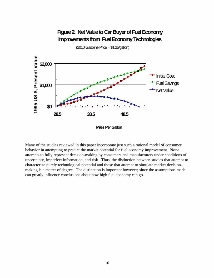
assumed that annual savings remained constant. These complications are frequently overlooked, resulting in considerable confusion about how to discount the present value of future fuel savings. Both the NEMS model and Energy and Environmental Analysis’ (EEA) Technology Cost Segment Model (TCSM) allow users to specify a discount rate and payback period. Most NEMS forecasts count only the first four years of fuel savings and use a real discount rate of 8 percent. This would be equivalent to discounting a constant rate of savings over 12 years at a rate of 28 percent per year. Studies using the TCSM have employed similar assumptions (EEA, 1988). If the intent is to predict the behavior of real-world markets, other factors come into play. The most important of these are: (1) dynamics, (2) risk, and (3) information. Dynamics are important because the implementation of a new automotive technology cannot be done instantaneously. It takes time to redesign vehicles for production and to prepare capital and labor for its production. There are institutional constraints, as well, such as the certification of vehicles to emissions, fuel economy and safety standards. Manufacturers’ own concerns about their reputations and product liability also require time for testing new designs. For these reasons, a new carline or major redesign requires 3-4 years from initiation to production. Manufacturers do not possess the resources to redesign all of their product lines at the same time, nor would they be willing under normal circumstances to undertake the risk. At current fuel prices, major fuel economy improvements across a manufacturer’s entire product line would be a very risky strategy because the potential pay-off is likely to be small relative to the risk incurred. Fuel economy improvements on the order of 30 percent and higher would require new body designs for improved aerodynamics, extensive materials substitution for weight reduction, as well as new engines and transmissions. If consumers decided they didn’t like the new vehicles, it could mean financial ruin for a manufacturer who elected to pursue that path alone. On the other hand, the net benefit to consumers of such sweeping changes is likely to be modest. In order to get higher fuel economy, consumers must pay a higher purchase price, the net benefit being the difference between the two. While the gross fuel savings from a 50 percent fuel economy improvement may easily exceed $1,000 in present value for a typical 28 mpg passenger car, the net value is unlikely to be more than $100 to $200, because of the cost of the fuel economy technology (Figure 2). If consumers dislike the look or feel of the new, more efficient designs, $100-200 is unlikely to compensate. Moreover, all of this assumes the consumer can accurately estimate the net present value of fuel savings. In reality, consumers are likely to be uncertain about the value of fuel savings. To estimate the net value of fuel economy improvements, consumers must have accurate information about the increase in fuel economy and its cost. While every new vehicle displays a label stating its fuel economy on a standard government test, the costs of fuel economy technologies are not available. Moreover, labeled MPG is several steps removed from the tangible benefit to the car buyer: avoided fuel costs. To estimate these at time of purchase, the consumer must factor in individual driving habits, traffic conditions, and future fuel prices to make the kind of rational decision envisioned by economic analysis.

16

Many of the studies reviewed in this paper incorporate just such a rational model of consumer behavior in attempting to predict the market potential for fuel economy improvement. None attempts to fully represent decision-making by consumers and manufacturers under conditions of uncertainty, imperfect information, and risk. Thus, the distinction between studies that attempt to characterize purely technological potential and those that attempt to simulate market decision-making is a matter of degree. The distinction is important however; since the assumptions made can greatly influence conclusions about how high fuel economy can go.

Figure 2. Net Value to Car Buyer of Fuel Economy Improvements from Fuel Economy Technologies

$0

$1,000

$2,000

28.5 38.5 48.5

Miles Per Gallon

1995

US

$, P

rese

nt

Val

ue

Initial Cost

Fuel Savings

Net Value

(2010 Gasoline Price = $1.25/gallon)

17

3. LITERATURE REVIEW U.S. transportation energy researchers have been studying the potential to increase fuel economy for more than 25 years. Early studies addressed the Corporate Average Fuel Economy (CAFE) Standards and the problem of U.S. oil dependence. For the most part, these analyses focused on what could be accomplished with proven technology over approximately a 10-year period. With growing concern over global climate change, some recent studies have addressed a longer time horizon and as yet unproven technologies. The basic methods of technology/cost analysis have changed little since the studies of the 1970s. 3.1 EARLY ASSESSMENTS: ENERGY CRISIS AND CAFE STANDARDS The potential to improve automotive fuel economy in the United States was first assessed in the early 1970s, motivated by concern over air pollution and the risks of increasing dependence on imported petroleum. In 1973 the first of these studies, Should We Have a New Engine? (Stephenson, 1975) was initiated by the Jet Propulsion Laboratory and the California Institute of Technology. Later that same year a boycott by members of the Organization of Petroleum Exporting Countries set off the first “energy crisis.” The crisis prompted Congress to enact the Energy Policy and Conservation Act (EPCA) of 1975, which mandated CAFE standards for passenger cars and light trucks. Several technology assessments were conducted to inform the development of the CAFE standards. Each enumerated technologies that could improve mpg, evaluated their potential applications, and estimated their costs (Coon, et al., 1974; Menchen et al., 1974; U.S. DOT/EPA, 1975a; 1975b). Impacts of individual technologies on fuel economy were estimated by a variety of methods, including engineering calculations, vehicle testing, computer simulation and paired comparisons of vehicles with and without a particular technology (e.g., Coon et al., 1974). The early studies recognized the need to consider technology interactions and the lead-time required for design changes. All of these studies were based on a specific set of proven technologies. While this provided the proof of feasibility and practicality for establishing fuel economy standards, it also necessarily limited the range of achievable mpg. The study by Menchen et al. (1974) appears to be the first to characterize “supply functions” for fuel economy, presented in the form of tables of retail price as a function of fuel economy level.4 The tables were organized by model year, to indicate what could be achieved over time, rather than organized by increasing marginal cost, as a supply curve. The data can be easily reordered by increasing marginal cost, however, to describe the cost of fuel economy improvements by 1982, as seen from the year 1974 (Figure 3). A subsequent report by many of the same authors, presented graphs of fuel economy potential in the form of cost curves which mapped the change in mpg against the total change in retail price (Curran et al., 1976).

4 Strictly speaking, a supply curve plots fuel economy improvement against marginal cost. However, most

technology/cost analyses plot the change in mpg versus the change in total retail price.

18

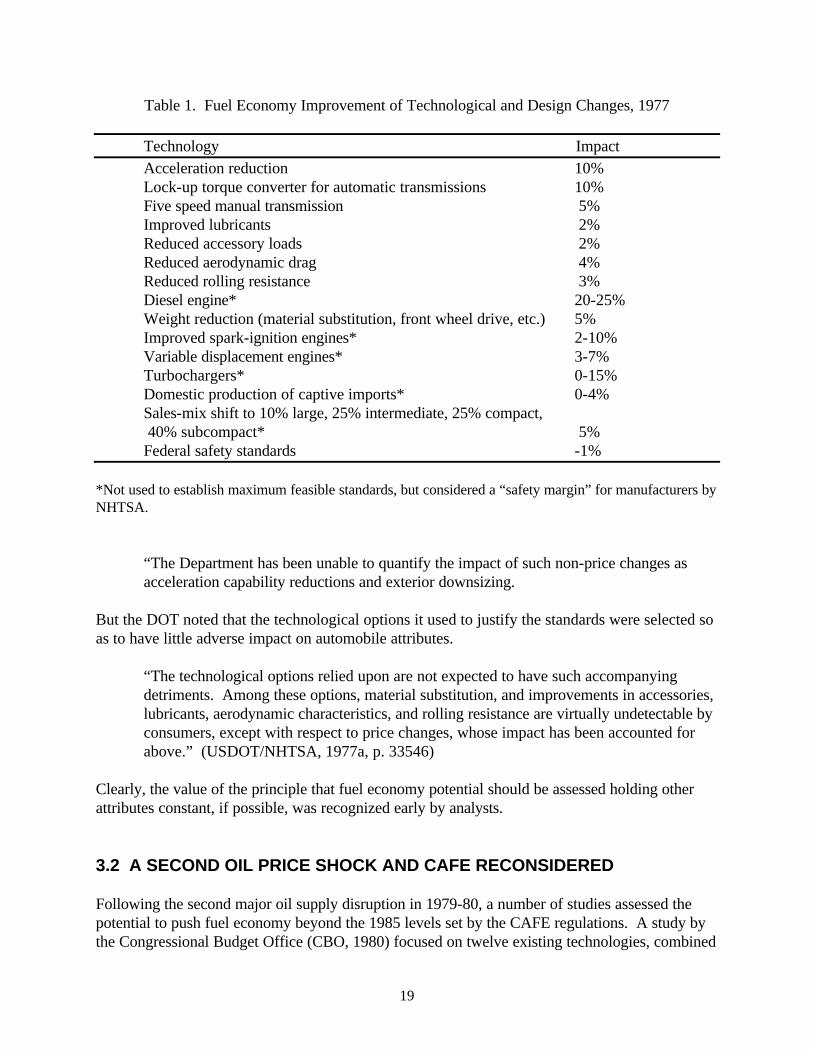
EPCA set mandatory fuel economy standards of 27.5 mpg for passenger cars in 1985, but allowed the U.S. Department of Transportation (DOT) to establish by rule passenger standards for the years 1981-84, and light truck standards for all years. The law required that the standards be set at the “maximum feasible” level, taking into consideration four factors: (1) technological feasibility, (2) economic practicability, (3) the effect of other Federal motor vehicle standards on fuel economy, and (4) the need of the nation to conserve energy. The rule-making responsibility necessitated additional studies to determine the technological and economic potential for increasing mpg. In a rule making establishing passenger car CAFE standards for 1981-84 the U.S. DOT evaluated manufacturers’ plans for downsizing and weight reduction along with the list of technologies shown in Table 1 (U.S. DOT/NHTSA, 1977a, 1977b). The DOT concluded that the goal of 27.5 mpg by 1985 was feasible, and also set standards for intermediate years. Similar assessments were carried out for light trucks, but over a shorter time horizon of two to three years into the future (U.S. DOT/NHTSA, 1978). While acknowledging the difficulty of accurately estimating costs, the DOT estimated that the impacts on vehicle prices would be minimal.

“The projected impact on new car prices,...is an increase of $54 by 1985, as an industry average, relative to 1977 model year automobiles.” (USDOT/NHTSA, 1977, p. 33546)

The DOT could not estimate the value of other attributes that might have to be changed to improve fuel economy.

Figure 3. "Supply Curve" for Fuel Economy: Subcompact Cars, 1974

$0

$100

$200

$300

$400

$500

$600

$700

20 22 24 26 28

MPG (60/40 Test Cycle)

Ret

ail P

rice

Incr

ease

(19

73 $

)

Total Cost

Marginal Cost

19

Table 1. Fuel Economy Improvement of Technological and Design Changes, 1977

Technology Impact Acceleration reduction 10% Lock-up torque converter for automatic transmissions 10% Five speed manual transmission 5% Improved lubricants 2% Reduced accessory loads 2% Reduced aerodynamic drag 4% Reduced rolling resistance 3% Diesel engine* 20-25% Weight reduction (material substitution, front wheel drive, etc.) 5% Improved spark-ignition engines* 2-10% Variable displacement engines* 3-7% Turbochargers* 0-15% Domestic production of captive imports* 0-4% Sales-mix shift to 10% large, 25% intermediate, 25% compact, 40% subcompact* 5% Federal safety standards -1% *Not used to establish maximum feasible standards, but considered a “safety margin” for manufacturers by NHTSA.

“The Department has been unable to quantify the impact of such non-price changes as acceleration capability reductions and exterior downsizing.

But the DOT noted that the technological options it used to justify the standards were selected so as to have little adverse impact on automobile attributes.

“The technological options relied upon are not expected to have such accompanying detriments. Among these options, material substitution, and improvements in accessories, lubricants, aerodynamic characteristics, and rolling resistance are virtually undetectable by consumers, except with respect to price changes, whose impact has been accounted for above.” (USDOT/NHTSA, 1977a, p. 33546)

Clearly, the value of the principle that fuel economy potential should be assessed holding other attributes constant, if possible, was recognized early by analysts. 3.2 A SECOND OIL PRICE SHOCK AND CAFE RECONSIDERED Following the second major oil supply disruption in 1979-80, a number of studies assessed the potential to push fuel economy beyond the 1985 levels set by the CAFE regulations. A study by the Congressional Budget Office (CBO, 1980) focused on twelve existing technologies, combined

20

with sales mix shifts to smaller cars. To the list in Table 1, the CBO study added only four-speed automatic transmissions, electronic engine controls, and lean-burn gasoline engines. The CBO study concluded that it was technologically feasible to achieve a fleet average fuel economy of 40 mpg by 1995. It estimated that a 27 percent increase from a fuel economy range of 27.5 to 31.0 mpg, to the range of 35 to 40 mpg would cost $600 to $654 per vehicle (1980 $). A 1980 study by the Mellon Institute (Shackson and Leach, 1980) appears to have been the first to include technologies (such as stirling engines) that were far from market-ready. The study’s methodology comprised four steps:

“(1) to characterize a baseline passenger car and light truck fleet in terms of weight, size classes, and the use of specific technologies; (2) to identify and characterize new technologies that could improve fuel economy during the next 20 years; (3) to construct for these technologies a likely implementation scenario, and (4) to compute new car fuel economy, the fleet fuel consumption, capital investment, consumer cost, and marginal cost of fuel saved.” (Shackson and Leach, 1980, p. 20)

New technologies considered by the Mellon Institute study included alcohol fueled vehicles, electric vehicles, and advanced combustion engines (turbine and stirling). The study concluded that without sales mix shifts, passenger cars could achieve 41.8 mpg by 1995 and 46.6 mpg by 2000. By assumption, “...half the improved efficiency obtained for cars was applied to new trucks.” It estimated that light trucks could reach only 22.2 mpg by 1995 and 23.5 by 2000. The Mellon Institute study presented annual consumer cost estimates for fuel economy technologies implemented in each year. It declined to estimate the cumulative costs of mpg improvements, however, noting that annual costs could not be simply added, since some technologies were replacing others previously added. The study did, however, estimate marginal costs of fuel economy improvement in terms of dollars per gallon saved in future years. It estimated that marginal costs would increase from about $0.50/gal. (1980 $) in 1980 to $1.30 to $1.80 in the late 1980s (with passenger car fuel economy at 37-39 mpg), up to $2.50 to $3.00 in the mid 1990s (at 41-44 mpg). Gray and von Hippel (1981) combined the “best available” technology for direct-injection turbocharged engines with continuously variable transmissions, lightweight materials (aluminum, fiber-reinforced plastics and foam-filled structures), aerodynamic drag and rolling resistance reductions to demonstrate potential improvements to 70 mpg for 4-passenger cars and 58 mpg for 5/6-passenger cars by 1995. With advanced technology, they foresaw mpg levels of 96 and 82, respectively. The 5/6-passenger car with 1980 best technology would have weighed 2,500 lbs., with a drag coefficient of 0.4. With advanced technology, its weight was to fall to 1,750 lbs., and Cd to 0.3. As for cost, Gray and von Hippel estimated that costs would remain below $1/gallon (1980 $) of fuel saved up to 60 mpg. All of the advanced technologies this study foresaw are in use in some mass-produced vehicle today, although not necessarily in ways that optimize fuel economy. In 1982, the U.S. Congress, Office of Technology Assessment (OTA, 1982) issued a study of several options for reducing U.S. oil imports, including increased automobile fuel efficiency.

21

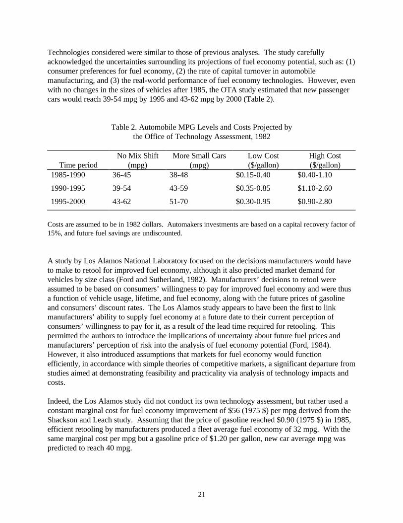
Technologies considered were similar to those of previous analyses. The study carefully acknowledged the uncertainties surrounding its projections of fuel economy potential, such as: (1) consumer preferences for fuel economy, (2) the rate of capital turnover in automobile manufacturing, and (3) the real-world performance of fuel economy technologies. However, even with no changes in the sizes of vehicles after 1985, the OTA study estimated that new passenger cars would reach 39-54 mpg by 1995 and 43-62 mpg by 2000 (Table 2).

Table 2. Automobile MPG Levels and Costs Projected by

the Office of Technology Assessment, 1982

Time period

No Mix Shift (mpg)

More Small Cars (mpg)

Low Cost ($/gallon)

High Cost ($/gallon)

1985-1990 36-45 38-48 $0.15-0.40 $0.40-1.10

1990-1995 39-54 43-59 $0.35-0.85 $1.10-2.60

1995-2000 43-62 51-70 $0.30-0.95 $0.90-2.80

Costs are assumed to be in 1982 dollars. Automakers investments are based on a capital recovery factor of 15%, and future fuel savings are undiscounted. A study by Los Alamos National Laboratory focused on the decisions manufacturers would have to make to retool for improved fuel economy, although it also predicted market demand for vehicles by size class (Ford and Sutherland, 1982). Manufacturers’ decisions to retool were assumed to be based on consumers’ willingness to pay for improved fuel economy and were thus a function of vehicle usage, lifetime, and fuel economy, along with the future prices of gasoline and consumers’ discount rates. The Los Alamos study appears to have been the first to link manufacturers’ ability to supply fuel economy at a future date to their current perception of consumers’ willingness to pay for it, as a result of the lead time required for retooling. This permitted the authors to introduce the implications of uncertainty about future fuel prices and manufacturers’ perception of risk into the analysis of fuel economy potential (Ford, 1984). However, it also introduced assumptions that markets for fuel economy would function efficiently, in accordance with simple theories of competitive markets, a significant departure from studies aimed at demonstrating feasibility and practicality via analysis of technology impacts and costs. Indeed, the Los Alamos study did not conduct its own technology assessment, but rather used a constant marginal cost for fuel economy improvement of $56 (1975 $) per mpg derived from the Shackson and Leach study. Assuming that the price of gasoline reached $0.90 (1975 $) in 1985, efficient retooling by manufacturers produced a fleet average fuel economy of 32 mpg. With the same marginal cost per mpg but a gasoline price of $1.20 per gallon, new car average mpg was predicted to reach 40 mpg.

22

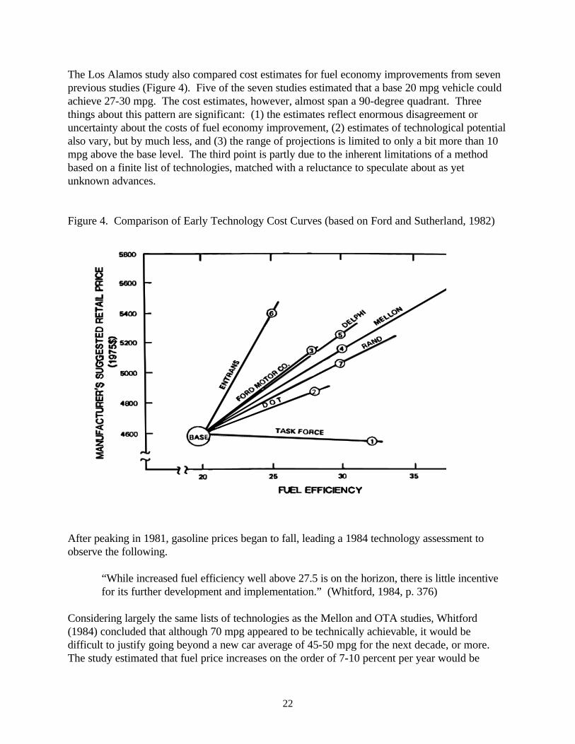
The Los Alamos study also compared cost estimates for fuel economy improvements from seven previous studies (Figure 4). Five of the seven studies estimated that a base 20 mpg vehicle could achieve 27-30 mpg. The cost estimates, however, almost span a 90-degree quadrant. Three things about this pattern are significant: (1) the estimates reflect enormous disagreement or uncertainty about the costs of fuel economy improvement, (2) estimates of technological potential also vary, but by much less, and (3) the range of projections is limited to only a bit more than 10 mpg above the base level. The third point is partly due to the inherent limitations of a method based on a finite list of technologies, matched with a reluctance to speculate about as yet unknown advances. Figure 4. Comparison of Early Technology Cost Curves (based on Ford and Sutherland, 1982)

After peaking in 1981, gasoline prices began to fall, leading a 1984 technology assessment to observe the following.

“While increased fuel efficiency well above 27.5 is on the horizon, there is little incentive for its further development and implementation.” (Whitford, 1984, p. 376)

Considering largely the same lists of technologies as the Mellon and OTA studies, Whitford (1984) concluded that although 70 mpg appeared to be technically achievable, it would be difficult to justify going beyond a new car average of 45-50 mpg for the next decade, or more. The study estimated that fuel price increases on the order of 7-10 percent per year would be

23

needed to produce a new car average mpg in the range of 40-45 by 2000. This rate of price escalation implies gasoline prices of $5-$9 (1998 $) per gallon in 2000. 3.3 DEPARTMENT OF ENERGY (DOE) STUDIES In 1978, the U.S. DOE began a series of studies assessing the ability of manufacturers to improve fuel economy. EPCA required DOE to advise the DOT on the technical feasibility and economic practicality of further fuel economy improvements, taking into consideration the need of the nation to reduce oil imports. Using the study by Hittman Associates (1976) as a starting point, the DOE and its contractor developed the Technology Cost Segment Model (TCSM) along with a technology data base, updated versions of which have been directly or indirectly used by virtually every assessment of fuel economy potential conducted in the past decade (EEA, 1979).5 The TCSM is a computer algorithm for assessing which fuel economy technologies will be adopted, determining their market penetrations, and calculating the resulting impacts on new vehicle fuel economy. It distinguishes among domestic manufacturers and vehicle size classes. The first step is to construct a data base of fuel economy technologies along with, (1) their fuel economy benefit as a percent increase over a baseline vehicle, (2) their costs in terms of increases in retail price, (3) the year in which the technology is first available for introduction, (4) maximum and minimum market penetrations, and (5) engineering notes containing information on technology synergies and interactions. Second, a database of existing market penetrations for all technologies by manufacturer and by vehicle class must be constructed to provide a starting point. The TCSM algorithm then proceeds year by year to select new technologies from the list of those available, basically in order of cost-effectiveness but taking other factors into consideration, as well. Although constant other vehicle characteristics is the default assumption, the TCSM simulates changes in vehicle weight and performance by defining these as “technologies” that may be adopted as a function of fuel price or according to a set schedule over time. The earliest version of the TCSM was designed to adopt technologies until an mpg target was met. Later versions (EEA, Inc., 1981), including that implemented in the NEMS Transportation Sector Model, estimate market shares as a function of cost-effectiveness and time since first introduction (DOE/EIA, 1994). Cost-effectiveness is defined as the value of fuel saved to the consumer, minus the increase in retail price of the vehicle. Once again the consumers’ willingness to pay for fuel economy improvement is assumed to be the driving factor in manufacturers’ decisions to adopt technologies and in the projection of fuel economy potential. In most of EEA’s analyses using the TCSM model, the net value of fuel savings to the consumer was estimated as savings over only the first four years of a vehicle’s life, discounted at an annual rate of 10 percent (EEA, Inc., 1986, p. 6-1). This choice of parameters seems to imply a failure on the part of used car markets to recognize the value of fuel economy improvements, but may also be

5This work was initiated and directed for nearly two decades by Barry D. McNutt of the U.S. Department of Energy, and carried out by K.G. Duleep of Energy and Environmental Analysis. Their influence on the evolution of data and methods in this area has been profound.

24

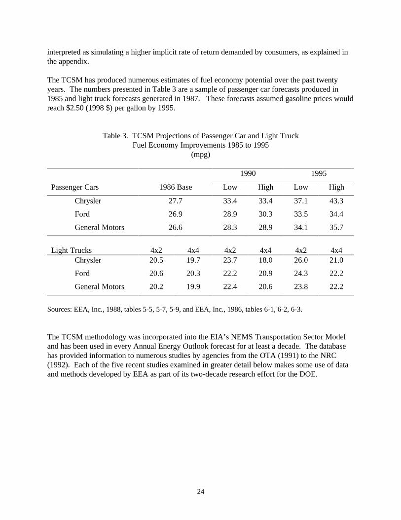
interpreted as simulating a higher implicit rate of return demanded by consumers, as explained in the appendix. The TCSM has produced numerous estimates of fuel economy potential over the past twenty years. The numbers presented in Table 3 are a sample of passenger car forecasts produced in 1985 and light truck forecasts generated in 1987. These forecasts assumed gasoline prices would reach $2.50 (1998 $) per gallon by 1995.

Table 3. TCSM Projections of Passenger Car and Light Truck Fuel Economy Improvements 1985 to 1995

(mpg)

1990 1995

Passenger Cars 1986 Base Low High Low High

Chrysler 27.7 33.4 33.4 37.1 43.3

Ford 26.9 28.9 30.3 33.5 34.4

General Motors 26.6 28.3 28.9 34.1 35.7

Light Trucks

4x2

4x4

4x2

4x4

4x2

4x4

Chrysler 20.5 19.7 23.7 18.0 26.0 21.0

Ford 20.6 20.3 22.2 20.9 24.3 22.2

General Motors 20.2 19.9 22.4 20.6 23.8 22.2

Sources: EEA, Inc., 1988, tables 5-5, 5-7, 5-9, and EEA, Inc., 1986, tables 6-1, 6-2, 6-3. The TCSM methodology was incorporated into the EIA’s NEMS Transportation Sector Model and has been used in every Annual Energy Outlook forecast for at least a decade. The database has provided information to numerous studies by agencies from the OTA (1991) to the NRC (1992). Each of the five recent studies examined in greater detail below makes some use of data and methods developed by EEA as part of its two-decade research effort for the DOE.

25

3.4 ADVANCED TECHNOLOGIES Analyses of fuel economy potential up to 1990 had been motivated by the need to establish or evaluate federal fuel economy regulations. Because of this, they were focused on a time horizon of a decade or less and generally restricted to proven technologies with minimal impacts on vehicle attributes other than cost and fuel economy. An overriding concern was to have a high degree of confidence that manufacturers could achieve fuel economy targets with minimal impact on their profitability. EEA (1990a) took a different approach. Looking 20 years ahead, it attempted to define a fuel economy “boundary” by considering the potential for technologies not ready for the market at that time. The change in perspectives was motivated by a growing consensus that something would have to be done about greenhouse gas emissions from motor vehicles, a problem with an inherently longer time horizon. Considering a longer time scale and including technologies not yet in production necessitated changes in methodology. One key change was to replace the technology/cost method with an engineering model of fuel economy. Another was the designation of “risk levels” in place of technology costs, which were considered too uncertain for an economic trade-off analysis. EEA (1990b) chose to evaluate fuel economy potential using a mathematical model of energy use over the federal test cycle. Technological impacts were described in terms of changes in the fundamental components of energy use, thermodynamic efficiency, conversion efficiency (e.g., engine friction and pumping losses), transmission efficiency, accessory power, mass, aerodynamic drag and rolling resistance. Building on engineering analyses of the federal test cycle by Sovran (1983) and Sovran and Bohn (1981), EEA derived fuel consumption elasticity estimates for each of these components and used them to estimate the impacts of technologies ranging from material substitution to hybrid drive. The elasticity estimates in Table 4 are interpreted as a percent change in fuel consumption (gallons per mile) for a 1 percent change in the factor in question, for a typical 1998 automobile with a mass of 1,400 kg. Thus, a 1 percent reduction in weight would permit a 0.64 percent reduction in fuel consumption, assuming constant acceleration performance. A 1 percent improvement in engine thermal efficiency would give a 1 percent reduction in fuel consumption. EEA’s analysis of “boundary” technologies did not estimate incremental costs, but did attempt to hold other vehicle characteristics approximately constant. Instead of estimating costs, it associated future fuel economy potentials with “risk levels”, described in terms of the likelihood that different technologies could be “commercialized” by 2010. Roughly, level 1 technologies were considered likely, level 2 uncertain, and level 3 unlikely but still possible. Risk level 1 technologies included extensive use of aluminum and plastics to achieve 18 percent lower mass, reductions in drag and rolling resistance and virtually universal use of 4-valve engines and variable valve controls. Risk level 2 added further weight reduction via even more aluminum plus graphite-reinforced plastics, further reductions in drag and rolling resistance, and use of turbo-charged direct injection (TDI) diesel engines in certain market segments. Risk level 3 added advanced emissions controls allowing universal use of TDI diesels, together with energy recovery and storage. The projected fuel economies achieved were 45 mpg for level 1, 55 mpg for level 2 and 74 mpg for level 3.

26

Table 4. Estimated Fuel Consumption (e.g., Gallons per Mile) Elasticities

Factor Elasticity Weight Reduction 0.54 (0.64)† Aerodynamic Drag (change in CD ) 0.22 Rolling Resistance (change in CR ) 0.23 Thermal Efficiency -1.00 Engine Pumping Losses 0.23 Engine Friction 0.23 Drivetrain Efficiency -0.78 Accessory Power 0.10 EEA, 1990b. †Includes downsizing of engine to maintain constant acceleration performance. Even the EEA “boundary” study’s approach was, like all previous fuel economy potential assessments, evolutionary and incremental, in that it began with a base year vehicle and accumulated technological changes to produce new designs of increasing fuel economy. Perhaps inspired by concept vehicles such as GM’s “ultralite,” Lovins et al. (1993) presented an assessment of what could be accomplished by radical design changes beginning with an essentially clean sheet. They argued that an ultralight vehicle weighing between 400 and 580 kg, with a drag coefficient of between 0.10 and 0.14, and a hybrid powertrain with regenerative braking, could achieve between 150 mpg and 300 mpg. Although many questioned the manufacturability, cost and marketability of such a vehicle, the concept of radically reinventing the automobile had already been gestating in automotive and energy policy circles. In early 1991, following the debates that yielded the new clean air regulations of 1990, including California’s zero-emission vehicle (ZEV) mandate, in the midst of the Persian Gulf war and proposals to strengthen the CAFE standards, Don Runkle, GM’s vice president of advanced engineering, proposed a joint government-industry research effort to solve the automobile’s energy, environmental, and safety problems within a decade’s time. Runkle called for a “moon shot” effort to develop breakthrough technologies, drawing an analogy to President Kennedy’s 1961 space race challenge that resulted in the successful 1969 moon landing (Keebler, 1991). Optimism about the potential for fuel efficiency breakthroughs centered on new powertrain technologies, especially hybrid drivetrains and fuel cells. In addition to Lovins’ concepts, less revolutionary but still substantial efficiency improvements using hybrid drive were identified in work by DOE, EPA, and a number of automakers and academics. In a prescient 1987 paper, Paul Werbos identified how fuel cell technology could transform the automobile and noted that a vigorous R&D effort would be needed to realize this potential (Werbos, 1987). Fuel cell R&D had continued to progress, particularly in fundamental work at Los Alamos National Laboratory and in engineering development by private industry. Kelly and Williams (1992) synthesized the rapid progress that was occurring in proton-exchange membrane (PEM) fuel cells with a renewed call for government-industry partnership. This idea then found ready acceptance in the new

27

Clinton/Gore administration, which put forward a “Clean Car Initiative” among a suite of technology initiatives proposed shortly after it took office in early 1993. After negotiations with industry, the Partnership for a New Generation of Vehicles (PNGV) was announced on September 29, 1993. This initiative established a cooperative research and development program between the federal government and the U.S. Council for Automotive Research (USCAR), whose members were Chrysler, Ford, and General Motors. One of the goals of the PNGV program is to develop technologies for an 80 mpg passenger car, with equivalent performance, size, utility, and cost to 1994 family sedan, while meeting or exceeding all federal safety and emissions standards (NRC, 1999). The establishment of PNGV and the greater recognition of the importance of technology breakthroughs, in contrast to refinement of known technologies, have significantly influenced the approaches taken by more recent studies of fuel economy potential. In addition to the EEA (1990) study, the OTA (1995) assessment and national-lab studies using NEMS have attempted to account for the potential progress due to PNGV and similar research efforts that accelerated during the 1990s. 3.5 ALTERNATIVE METHODS Not all studies of the potential for improving light duty vehicle efficiency conducted over the past twenty-five years have relied on technology/cost analysis or engineering simulation models. Alternatives range from “Best-in-Class” to regression analysis (Table 5). Because not all the alternative methods explicitly link tangible technologies to fuel economy improvement, they are less useful as a “proof” of feasibility and economic practicality. On the other hand, some studies have employed multiple approaches in the belief that one can have greater confidence if the same general result can be obtained by several different methods (e.g., NRC, 1992).

Table 5. Methodologies for Assessing Potential Fuel Economy Improvements

• Best-in-class (BIC) analysis of the existing fleet: NRC (1992); Heavenrich and Hellman (1996); DeCicco (1997).

• Regression analysis of fuel economy differences in the existing fleet: Berger et al. (1990). • Assessments citing high-efficiency concept vehicles: Bleviss (1988); EEA (1990). • Delphi studies, based on expert opinions: OSAT (1990), OSAT (1998) • Technology menu ("shopping cart") analysis: Difiglio et al. (1990); Ledbetter and Ross

(1990); Greene and Duleep (1993); DeCicco and Ross (1993). • Engineering modeling: EEA (1990); DeCicco and Ross (1993); Ross (1994); OTA (1995,

summarized in Duleep 1997); Lovins (1995). A "best-in-class" analysis examines fuel economy leaders in the fleet of a given model year, controlling for attributes according to some class definition. For example, Heavenrich and Hellman (1996) use a best-in-weight-class analysis to identify a potential 10 percent increase in

28

light vehicle fuel economy relative to the 1996 new fleet. To date, cost impacts have not been estimated in a best-in-class analysis. A more significant shortcoming of the Best-in-Class method is the difficulty of holding vehicle attributes, other than those that define the classes, constant. Classifications based on size or market intent generally have significant variations in weight, engine size, acceleration, transmission type and accessories among carlines. “Best” fuel economy vehicles tend to be lighter, lower power, manual transmission models, with minimal accessories. Defining classes that hold most important attributes constant generally leads to too few vehicles per class to be meaningful. As a result, best-in-class analysis tends to confound technology costs with the costs of trading-off other amenities for fuel economy and is not useful for developing cost estimates. Berger, et al. (1990b) statistically estimated the impacts of variables such as vehicle weight, engine power, engine displacement, etc., on fuel economy by means of regression analysis. They then used their regression model, in combination with an engineering analysis, to predict a potential 13 percent automobile fuel economy improvement by 2000, relative to the 1988 fleet. The engineering analysis was required to hold other attributes, such as ride quality, noise, vibration and harshness constant. Regression analyses are limited by two factors: (1) only technologies deployed on a sufficient number of vehicles to produce a statistically significant result can be included (correlations among key variables such as weight and engine size and difficulties in measuring other key factors complicate this problem), and (2) there is only limited ability to control for the manufacturer’s intent in implementing a particular technology. Some key fuel economy technologies (e.g., 4-valves per cylinder and variable valve timing and lift control) can have very different impacts depending on whether the design goal is to improve fuel economy or performance. Regression analysis has not been successfully used to estimate the costs of fuel economy technologies. Nonetheless, regression analysis can be useful in that it provides another source of empirical estimates of technology impacts. Analogous pitfalls can restrict the value of extrapolating from high-efficiency prototypes. Not only is it difficult to hold other attributes constant, but concept vehicles often do not include all of the design elements required in a marketable vehicle. By the mid-1980s a number of concept cars had been built demonstrating fuel economies that were double the U.S. car average of 28 mpg. Bleviss (1988) provides a list of such high-efficiency vehicles, as have several other studies such as EEA (1990b). Frequently, the concept cars had not been certified to federal emissions or safety standards. In effect, such vehicles represent a “proof” that vehicles with very high fuel economy can be built, but with certain changes in vehicle attributes that may or may not pass the test of the marketplace. Delphi methods summarize and draw inferences from in-depth surveys of expert opinion in the automotive industry, supplier firms, consultants, and others. Although subjectivity is inherent, both in the design and responses, Delphi surveys still provide important insights and are a source of supporting evidence for fuel economy projections based on more rigorous methods. The University of Michigan's Office for the Study of Automotive Transportation (OSAT) has conducted a series of such studies, most recently OSAT (1998). Although earlier studies, such as OSAT (1990?) did project potential fuel economy levels, recent studies have not made projections, examining instead the technological implications of various near-term fuel economy

29

levels. Delphi methods, however, provide no clear blueprint of how fuel economy improvements can be achieved. In addition, it is rarely clear what assumptions about technological progress, economic conditions, and other factors underlay the respondents’ answers.

30

31

4. REVIEW OF SIX RECENT STUDIES As noted earlier, the work of K.G. Duleep and colleagues at EEA, commissioned largely by the U.S. DOE, has been a cornerstone of U.S. studies addressing light vehicle fuel economy for two decades. Several other organizations have published their own analyses of the subject, but all build to a greater or lesser degree on the work by EEA. We review six studies in this section, listed below according to the lead organizations involved: EEA Energy and Environmental Analysis, Inc., carried out studies for the DOE, EPA, OTA, and others. ACEEE American Council for an Energy-Efficient Economy, derived from EEA studies by adding certain technologies and making alternative assumptions. NRC National Research Council (NRC) considered EEA and automotive industry analyses. OTA U.S. Congress, Office of Technology Assessment, used EEA as a contractor but also received advice and review from a panel of experts. EIA Energy Information Administration (an independent statistical agency within DOE), used EEA as the prime contractor for the automotive modules of the National Energy Modeling System (NEMS). NL/DOE National Laboratories, used NEMS and added certain technologies and alternative assumptions. EEA was a contractor. 4.1 EEA STUDIES Analyses performed with EEA’s (1985, 1991) TCSM have been used in a large number of government-sponsored studies (e.g., Difiglio et al. 1990; and Greene and Duleep 1993). EEA's TCSM tracks vehicle characteristics and technologies at the carline level of detail, where a carline is defined as a given manufacturer's products in a given market segment (e.g., Ford's midsize cars, GM's subcompact cars, etc.). Historically, emphasis was place on the capabilities of the U.S. domestic automakers (the traditional "Big 3"), who are most constrained by CAFE standards. The TCSM permits separate analysis of domestic vs. import fleets permitting assessment of the differential impacts of higher fuel economy levels. Representative results from EEA studies of the late 1980s were reported by Difiglio, Duleep, and Greene (1990; "DDG"). They worked from a 1987 base year and developed three scenarios for domestic automobiles (passenger cars only) in 2000, summarized in Table 6. All scenarios assumed size and performance fixed at the 1987 fleet average level. The Product Plan and Cost-Effective scenarios were based on technologies that might be incorporated on the basis of fuel savings, assuming a retail gasoline price of $1.32/gallon (1987$ in 2000, including taxes), according to differing payback periods discounted at 10 percent per year. A Maximum Technology scenario assumed use of all technologies identified in that version of EEA's TCSM regardless of cost. DDG also noted that levels 1-2 mpg higher could be obtained by relaxing the fixed-size assumption and allowing some shifts to smaller cars.

32

Table 6. Difiglio, Duleep, and Greene (1990) Summary Results

Scenario (for domestic cars)

New Car Fleet MPG

Percent Increase

Cost Increase (1987$)

1987 Base Year Fleet 27.0 -- --

2000 Product Plan (payback in 4 years) 34.3 27% $373

2000 Cost-Effective (payback in 10 years) 36.4 35% $493

2000 Maximum Technology 39.5 46% $757

A 1991 study by the Office of Technology Assessment (OTA) also used EEA as contractor. The OTA (1991) estimate of the new automobile fleet fuel economy achievable by 2001 under “regulatory pressure” was 35.5 mpg, assuming constant 1990 size and performance and 10-year payback at $2.00/gal fuel price. This result was spanned by a “product plan” projection of 32.9 mpg and a “maximum technology” estimate of 38.2 mpg. Drawing on EEA (1990), OTA (1991) also estimated what might be achievable by 2010 using advanced technologies, reporting a range of 45 mpg to 55 mpg depending on current engineering opinions about what would be commercialized in a post-2000 time frame. Greene and Duleep (1993; "G&D") published an updated analysis as part of a broader examination of the economic impacts of fuel economy improvement. Working from a 1988 base year, the analysis defined three scenarios for 2001, summarized in Table 7. The Base Case was defined similarly to the Product Plan of DDG. A Level 3 scenario used Maximum Technology assumptions, and a Level 2 scenario used assumptions intermediate between the Base Case and Level 3. G&D developed projections for light trucks as well as passenger cars, and for the domestic, import, and combined fleets. They found a somewhat lower degree of potential efficiency improvement for light trucks compared to cars. The main reason is that, under the EEA TCSM assumptions, some technologies (such as front wheel drive, 4-valve engines) are not as widely applicable in light trucks as they are in cars. Compared to the DDG results, the G&D results suggest that a lower degree of efficiency improvement is possible for a given cost over a similar, decade-long time frame. For domestic passenger cars, for example, the G&D Max Tech results imply a 35 percent fuel economy gain for $995, compared to the DDG Max Tech results of a 46 percent for $788 (both in 1988$). The cost to achieve a given degree of fuel economy improvement is roughly 70 percent higher for the G&D study. A key reason is that a portion of the technology potential available in 1987 was absorbed into the fleet by 1990 but used to increase mass, power, and performance rather than fuel economy. Projecting forward to 2001, even the G&D Max Tech case involves a modest performance improvement, as indicated by increases in the horsepower to weight ratio of about 8

33

percent for cars and 5 percent for light trucks. The G&D study also made adjustments for safety feature improvements.

Table 7. Greene and Duleep (1993) Summary Results for Domestic Fleet

New Passenger Cars New Light Trucks

Scenario (costs in 1988$) MPG % Increase Cost MPG % Increase Cost

1990 Base Year Fleet 26.6 -- -- 20.3 -- --

2001 Base Case (Prod Plan) 31.8 20% $633 23.4 15% $350

2001 Level 2 34.2 29% $713 25.2 24% $610

2001 Level 3 (Max Tech) 35.8 35% $995 26.7 32% $1020

4.2 ACEEE STUDIES The ACEEE has published a series of studies using much of the EEA TCSM data but with more optimistic assumptions regarding technology (Ledbetter and Ross 1990; DeCicco and Ross 1993, 1996). ACEEE's analyses used an aggregated version of EEA's TCSM, so that a single technology matrix represents the entire U.S. passenger car fleet (all carlines combined, not separately treating the domestic and import fleets). ACEEE's analysis accounted for a multiplicative interaction (positive synergy) between drivetrain (engine, transmission) and tractive load (mass reduction, streamlining, etc.) technologies, which are treated in an additive fashion by EEA. It also allows higher maximum market penetration rates for some technologies, as well as lower technology costs in certain cases. As noted above, the EEA analyses report different scenarios according to cost-effectiveness assumptions. The ACEEE studies also varied the technologies available and the extent of their possible utilization, prior to applying cost-effectiveness criteria. Working from a 1987 base year, Ledbetter and Ross examined two future years, 2000 and 2010, with an expanded technology set in the latter year. Working from a 1990 base year, DeCicco and Ross examined a single time horizon, which they placed at 2002-2005 based on an examination of lead-time requirements from their year of analysis. They examined three levels of technology risk and two levels of technology utilization (referring to each technology's maximum fleetwide penetration). One level of technology utilization was the same as used by EEA; the other level was higher, based on the authors' judgments of the maximum level technically possible without exceeding limits based on past observed deployment rates for similar technologies. Table 8 summarizes results from their 1996 paper based on an average of the two utilization levels and cost-effectiveness using a 5 percent real discount rate and 12-year vehicle lifetime, compared to a retail gasoline price of $1.65/gal (1993$ in 2005).

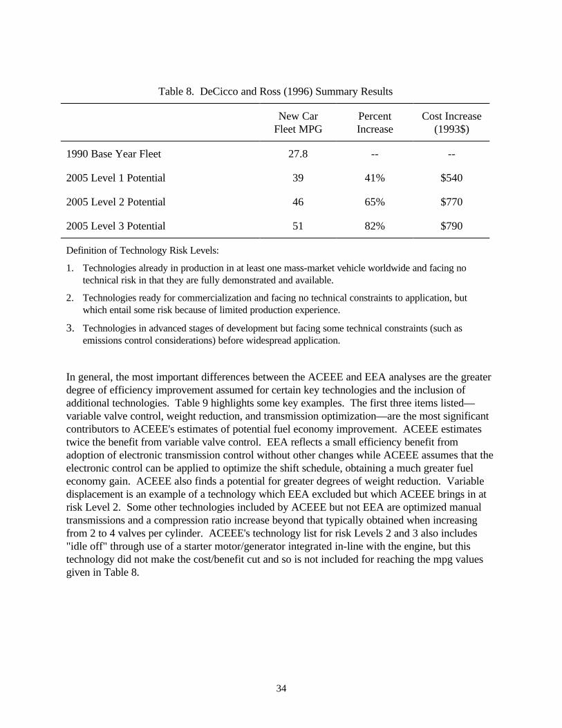
34

Table 8. DeCicco and Ross (1996) Summary Results

New Car Fleet MPG

Percent Increase

Cost Increase (1993$)

1990 Base Year Fleet 27.8 -- --

2005 Level 1 Potential 39 41% $540

2005 Level 2 Potential 46 65% $770

2005 Level 3 Potential 51 82% $790

Definition of Technology Risk Levels:

1. Technologies already in production in at least one mass-market vehicle worldwide and facing no technical risk in that they are fully demonstrated and available.

2. Technologies ready for commercialization and facing no technical constraints to application, but which entail some risk because of limited production experience.

3. Technologies in advanced stages of development but facing some technical constraints (such as emissions control considerations) before widespread application.

In general, the most important differences between the ACEEE and EEA analyses are the greater degree of efficiency improvement assumed for certain key technologies and the inclusion of additional technologies. Table 9 highlights some key examples. The first three items listed—variable valve control, weight reduction, and transmission optimization—are the most significant contributors to ACEEE's estimates of potential fuel economy improvement. ACEEE estimates twice the benefit from variable valve control. EEA reflects a small efficiency benefit from adoption of electronic transmission control without other changes while ACEEE assumes that the electronic control can be applied to optimize the shift schedule, obtaining a much greater fuel economy gain. ACEEE also finds a potential for greater degrees of weight reduction. Variable displacement is an example of a technology which EEA excluded but which ACEEE brings in at risk Level 2. Some other technologies included by ACEEE but not EEA are optimized manual transmissions and a compression ratio increase beyond that typically obtained when increasing from 2 to 4 valves per cylinder. ACEEE's technology list for risk Levels 2 and 3 also includes "idle off" through use of a starter motor/generator integrated in-line with the engine, but this technology did not make the cost/benefit cut and so is not included for reaching the mpg values given in Table 8.

35

Table 9. Differences Between EEA and ACEEE Assumptions for Some Key Technologies for Improving Fuel Economy

Discrete MPG Benefit*

EEA ACEEE

Technology (NRC high) Level 2 Level 3

Variable Valve Control 6% 12% 12%

Weight Reduction 7% 10% 16%

Transmission Optimization 0.5% 9% 9%

Engine Friction Reduction 3% 6% 6%

Tire Improvements 1% 5% 6%

Variable Displacement -- 5% 5%

Lean Burn -- -- 10%

*Discrete benefit refers to that of a technology applied to a base year vehicle without adjusting for fleetwide utilization levels.

Lean burn is a risk Level 3 technology that faces constraints due to NOx control difficulties. It does make the cost/benefit cut, and is the largest factor in moving from ACEEE's Level 2 to Level 3 estimates. ACEEE treated lean-burn as representing a number of distinct engine options which use lean (rather than stoichiometric) air/fuel mixtures. For example, the lean-burn engine in Honda’s VX coupe in Model Years 1992-95 uses a variable valve control mechanism to help attain a high-swirl, highly stratified charge. Two-stroke engines also run lean. They looked promising in the early 1990s and ACEEE considered them to be another approach for achieving the same efficiency benefit. ACEEE did not include the direct injection spark ignition (DISI) approach, also known as direct injection stratified charge (DISC), yet another lean burn engine which is now used in several vehicles sold in Japan. None of these lean burn technologies were included in EEA’s conventional analyses as discussed above. 4.3 NATIONAL RESEARCH COUNCIL (1992) In 1991, the U.S. DOT requested the NRC to undertake “…a study of the potential and prospects for improving the fuel economy of new light-duty vehicles.” (NRC, 1992, p. vii) The NRC convened a committee that was charged to provide estimates by vehicle size class, of fuel economy levels that could be practically achieved in new automobiles and light trucks over the

36

next decade. The report was the first to consider in an integrated format a full range of safety, environmental, and economic issues related to improving fuel economy. The study used two other methods in addition to technology cost analysis to project future fuel economy levels. The committee clearly stated that it considered the results of all three approaches in arriving at a range of “consensus” estimates. The first method presented is simply trend extrapolation, based on both miles per gallon and ton-miles per gallon for light-duty vehicles from 1975 to 1991. The ton-mpg measure was intended to remove weight as a consideration, thereby focusing on engine, drivetrain, aerodynamic and rolling resistance improvements. For passenger cars, historical trends in mpg and ton-mpg indicated improvements of 0.71 mpg/yr. and 0.45 mpg/yr., respectively. For light trucks the corresponding rates of mpg increase were 0.45 mpg/yr. and 0.4 mpg/yr. From the committee’s viewpoint, the trend analysis indicated that such rates might be achievable in the future, since they had been achieved in the past. The committee also carried out a Best-in-Class (BIC) analysis for passenger cars and light trucks by size class. The BIC index was defined as the average fuel economy of the top mpg carlines that together accounted for at least 5 percent of total sales within a class. The resulting BIC numbers are as follows: subcompact: 47.2 mpg; compact: 33.4 mpg; midsize: 27.7 mpg; large: 24.3 mpg; small pick-up: 27.1 mpg; small van: 24.3 mpg; large pick-up: 26.3 mpg; small utility vehicle: 29.8 mpg. The committee noted that there was a much smaller range of fuel economy in the midsize and large size classes than in the subcompact and compact classes, and suggested that there might be less competition on fuel economy in the larger car classes. The NRC study also carried out its own version of a classic technology/cost analysis, which it termed the “shopping cart” approach. Its key assumptions were: (1) only proven technologies were considered, (2) other vehicle attributes were held constant at 1990 levels, (3) weight reduction in the form of conversion to front-wheel drive and 10 percent weight reduction via materials substitution were permitted, (4) maximum market penetrations were assumed to be 100 percent unless there were compelling reasons to assume otherwise, (5) positive and negative synergies were neglected, and (6) all safety and emissions regulations must be met. Two sources of data on technology impacts and costs were used: the latest estimates by EEA, Inc. for the U.S. DOE and a study by SRI, Inc. (NRC, 1992, p. 137 and appendix B).6 The NRC study found the greatest discrepancies between the two data sources were in the cost estimates, rather than the technology impacts. It attributed a large part of the differences to SRI’s assumption that fuel economy improvements would require premature retirement of capital equipment versus EEA’s assumption of long-run marginal costs. Both studies measured cost in terms of changes in retail price. Results were summarized in the form of curves plotting retail price increase versus miles per gallon for four car and four light-truck types. In general, the data provided by EEA indicated that fuel economy levels two or more mpg beyond those estimated by the SRI data could be achieved at less than half the cost. 6 The NRC study cites a personal communication from K.G. Duleep as its source of EEA data and a report

by SRI that bears the label “Client Private”. We cite neither of these sources here, but only the NRC report.

37

Based on these analyses, and the expert judgments of the committee, the NRC study decided upon a range of “technically achievable” fuel economy estimates and costs for the year 2006 (Table 10). The committee expressed its uncertainty in the form of high and low confidence estimates for fuel economy and price. The high and low confidence price estimates themselves are expressed as ranges, so that the final results are parallelograms in cost-mpg space. It seems clear that the SRI-EEA data differences strongly influenced the committee’s thinking. In the absence of compelling evidence to resolve these differences, the committee reflected them in its conclusions.

Table 10. “Technically Achievable” Fuel Economy for MY 2006 Vehicles

Ranges of “Technically

Achievable” Fuel Economy in MY 2006

(mpg)

Incremental Retail Price Equivalent for Improved

Fuel Economy in MY 2006 (1990 Dollars)

Vehicle Size Class

Higher

Confidence

Lower

Confidence

At Higher Confidence

Fuel Economy

At Lower Confidence

Fuel Economy

Passenger Cars

Subcompact 39 44 500–1,250 1,000–2,500

Compact 34 38 500–1,250 1,000–2,500

Midsize 32 35 500–1,250 1,000–2,500

Large 30 33 500–1,250 1,000–2,500

New car fleet 34 37

Light Trucks

Small pickup 29 32 500–1,000 1,000–2,000

Small van 28 30 500–1,250 1,000–2,500

Small utility 26 29 500–1,250 1,250–2,500

Large pickup 23 25 750–1,750 1,500–2,750

New light truck fleet 26 28 Source: National Research Council (1992), table 8-1.

38

4.4 OFFICE OF TECHNOLOGY ASSESSMENT (1995) Prompted by the Congress’ desire for a technical assessment of the President’s Partnership for a New Generation of Vehicles initiative, the Office of Technology Assessment (OTA, 1995a&b) undertook an evaluation of the performance and costs of a range of advanced vehicle technologies that it considered likely to be available during the next 10 to 20 years. Unlike previous technology/cost analyses, the study focused directly on unproven technologies. Two requirements for advanced vehicles were that their acceleration and hill climbing performance be equivalent to those of 1995 gasoline vehicles, and that they be mass producible in volumes of hundreds of thousands per year. Rather than consider all kinds of light-duty vehicles, the OTA study focused on a range of technologies applied to mid-size passenger cars. In addition to a baseline vehicle, three technology types were evaluated for the years 2005 and 2015: (1) advanced conventional, (2) battery electric vehicles, and (3) hybrid-electric vehicles. Technologies for advanced conventional vehicles included reducing tractive forces and improving engine efficiency. The OTA assessment assumed that current drag coefficients of 0.33 could be reduced to 0.25 or, more optimistically, to 0.22. Advanced tires with rolling resistance coefficients (RRC) 30 percent lower than today’s levels of 0.008-0.010 were considered possible by 2005, with a further reduction to 0.005 by 2015. Weight reduction was a key technology for conventional vehicles. OTA estimated that optimized steel-body vehicles with aluminum engines could achieve a 15 percent weight reduction by 2005. Adding more aluminum to the body could push that to 20 percent. A “clean sheet” optimized aluminum design could achieve a 30 percent weight reduction by 2015 and, if severe manufacturing challenges could be overcome, substituting carbon fiber composites might reduce mass by 40 percent. Engine improvements were judged equally important to fuel economy gains for advanced conventional vehicles. Continued improvements to baseline 4-valve per cylinder engines could yield fuel economy improvements of up to 15 percent. In comparison to a baseline engine, direct-injection gasoline engines (a lean-burn technology) were judged to offer a 22 to 33 percent fuel economy advantage, if nitrogen oxide emissions problems could be solved. Finally, 4-valve direct-injection diesel engines could boost mpg by 40 percent over the baseline engine, again assuming that emissions problems could be solved (30 percent efficiency improvement taking the higher energy content of diesel fuel into account). OTA summed up the combined potential of these technologies as follows (OTA, 1995, p. 11): “If OTA’s projections for technology prove to be correct, a mid-size auto could achieve 39 to 42 mpg by 2005 and 53 to 63 mpg 2015 using these technologies, at a net price increase to the buyer of $400 to $1,600 in 2005 and $1,500 to $5,200 in 2015.” OTA also considered electric vehicles because they are the only technology capable of meeting the California Zero Emission Vehicle mandates. The key issue is the cost and performance of batteries. Advanced battery designs considered included nickel metal hydride, lithium polymer and lithium ion. The study concluded that by 2015 a midsize EV might achieve energy efficiencies on the order of 50 mpg gasoline equivalent using advanced lead-acid technology, or

39

more than 80 mpg with nickel metal hydride technology, but would likely cost $4,000-$10,000 more than a conventional vehicle and still have limited range. The OTA study also considered the potential of hybrid technologies, which it concluded would offer up to a 30 percent improvement over an otherwise identical gasoline vehicle, if advances in storage devices and other electrical components could be achieved. By 2005, OTA judged that a midsize hybrid with a 37 kW engine, an advanced lead-acid battery and an optimized steel body could achieve 49 mpg, but would cost $4,900 more than a conventional vehicle. By 2015, a similar vehicle with an optimized aluminum body and other advances might reach 65 mpg, but at an incremental cost of $4,600. The OTA study’s cost and mpg conclusions are summarized in Tables 11 and 12. OTA’s estimates of technology impacts and costs were derived primarily by K.G. Duleep of EEA, Inc., using the mathematical modeling approach first introduced in the 1990 “boundary” analysis, described above. A panel of experts reviewed estimates. The method was, in effect, a combination of engineering modeling and Delphi survey.

Table 11. 2005 Model Year Midsize Car

Vehicle type

Body Material

Fuel Economy,

mpg

Price Change, $

Comments

Business as usual Baseline steel 30 Base

Advanced conventional

Optimized steel 1st generation aluminum

39 42

+400 +1,600

Electric vehicle (EV)

Optimized steel Optimized steel

31 48

+11,400 +18,400 (9,300)

Lead acid battery NiMH battery (lower price assumes battery cost $200/kWh, based on developer claims)

Hybrid-electric Optimized steel 1st generation aluminum

49

61

+4,900 +7,800/10,200

Bipolar lead acid battery energy storage Flywheel/ultra-capacitor energy storage

Source: OTA, based on EEA’s “Automotive Technologies to Improve Fuel Economy to 2015,” prepared for the OTA, June, 1995. Some aspects of technology now seem to be progressing more rapidly than foreseen by either the OTA or EEA advanced technology assessments. For example, OTA (1995) projected that optimized aluminum structures might cut vehicle body mass by 30 percent by 2015. However, Ford has built a small test fleet of aluminum-intensive prototypes and reported extensive progress in structural optimization with aluminum, achieving a 40 percent weight reduction in current

40

prototypes and seeing a potential for a 50 percent reduction compared to current steel unibodies (Cornille et al., 1998). Hybrid drivetrain technology has clearly advanced more rapidly than anticipated by EEA (1990) or OTA (1995). The Toyota Prius has been available in Japan since December 1997, with cumulative sales exceeding 25,000 by mid-1999; it is slated for U.S. and European sales in mid-2000. The Honda Insight is being introduced for retail sale in the U.S. market for model year 2000. Relative to vehicles of similar size and performance, these first commercial hybrids achieve fuel economy improvements comparable that of the 49 mpg midsize car estimates by OTA (1995). However, costs, and therefore the long-term prospects, are still uncertain. For example, it remains unclear whether technologies such as aluminum unibodies and hybrid drivetrains can be profitable in high volume products throughout the market.

Table 12. OTA’s Estimate of Technology Impacts and Costs for a 2015 Model Year, Midsize Car

Vehicle type

Body

Material

Fuel Economy,

mpg*

Price Change,

$

Comments Business as usual

Optimized steel 33 Base

Advanced conventional

Optimized aluminum Carbon fiber composite

53 64

+1,500 +5,200

DISC engine Price extremely uncertain

Electric vehicle Optimized aluminum Optimized aluminum

51 82

+4,200 +10,300/4,300

Lead acid battery NiMH battery (lower value assumes battery cost $180/kWh)

Hybrid-electric Optimized aluminum Optimized aluminum

65

71-73

+4,600 +7,000/9,800

Bipolar lead acid battery energy storage Flywheel/ultra-capacitor energy storage

Fuel cell hybrid Optimized aluminum 83 +6,000/40,000

Lower price assumes major cost breakthroughs ($65/kW); energy storage by bipolar lead acid battery

* Gasoline-equivalent miles-per-gallon, based on primary energy consumption for electricity, and lower heating value for fuel cell vehicles, which are assumed to use methanol fuel. Source: OTA (1995, p. 42). The OTA (1995) study gave very limited consideration to fuel cell vehicles, reflecting the view that the technology was still in early stages of development. OTA concluded that high-volume automotive applications were very unlikely by 2005 and still speculative for even 2015. Subsequently, R&D investment by automakers and engineering development of fuel cell stack technologies has progressed significantly (FCTAP, 1998). Daimler-Chrysler and Ford have both demonstrated fully functional fuel cell concept vehicles, and all major automakers have announced

41

at least demonstration-scale early commercialization programs for a 2004 time frame. However, major barriers still remain for many aspects of the technology (Stobart, 1999). Moreover, no known fuel cell technology can operate directly on gasoline or diesel fuel. Unlike refinements to conventional vehicles or even hybrid drive, fuels cells face added barriers due to this fuel issue, requiring either additional technology development (and costs and complications) for fuel reforming or infrastructure development for hydrogen or methanol. Nevertheless, progress on fuel cell technology has generated a wave of optimism about future fuel economy potential. Ogden et al. (1999) estimate a range of 69 mpg to 106 mpg (gasoline equivalent, depending on the fuel) for a mid-size sedan. The time frame for commercialization of automotive fuel cells is still uncertain, but the active development work by auto companies reflects a belief that this technology can become affordable in the long run. It is just such technological progress that is so difficult to capture in engineering-economic studies such as those reviewed here. 4.5 “5-LAB” STUDY (1997) In 1997 the DOE convened a study group comprised of researchers from five of its national laboratories to measure the potential for energy efficient and low-carbon technologies to reduce carbon emissions from the United States by 2015 (Interlaboratory Working Group, 1997). Using the EIA’s NEMS model as an integrating framework, the study assessed the impacts of advanced technologies in all economic sectors. Two advanced technology scenarios were considered, in addition to a base case, which was a slightly modified version of the EIA’s 1998 Annual Energy Outlook (AEO) forecast. The Efficiency (EFF) Scenario was intended to represent “reasonable, incremental assumptions” about the effects of a concerted effort to accelerate the development and promote the adoption of advanced technologies. The High-Efficiency/Low-Carbon Scenario was characterized as a more optimistic version of the Efficiency Scenario, and postulated technological breakthroughs in key areas such as fuel cell systems. The list of automotive technologies considered by the 5-Lab study included all the conventional technologies available in the 1998 AEO, plus six others shown in Table 13. The prices assumed for these technologies are lower than those assumed in OTA (1995), and their introduction dates have been accelerated, especially in the High-Efficiency Scenario. Direct-injection, stratified charge (DISC) engines were assumed to be available in the United States in 2000; it now appears that they will not be available in 2000 due to difficulty meeting U.S. emissions standards. Several DISC engine configurations are available in Japan, however. Both the price and efficiency gain for the gasoline fuel cell vehicle is heroic in comparison to the OTA study’s estimates.

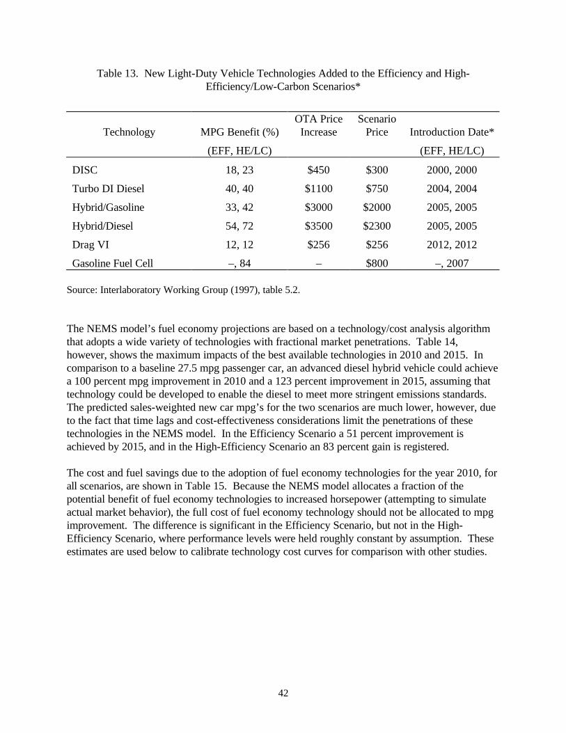
42

Table 13. New Light-Duty Vehicle Technologies Added to the Efficiency and High-Efficiency/Low-Carbon Scenarios*

Technology MPG Benefit (%) OTA Price

Increase Scenario

Price Introduction Date*

(EFF, HE/LC) (EFF, HE/LC)

DISC 18, 23 $450 $300 2000, 2000

Turbo DI Diesel 40, 40 $1100 $750 2004, 2004

Hybrid/Gasoline 33, 42 $3000 $2000 2005, 2005

Hybrid/Diesel 54, 72 $3500 $2300 2005, 2005

Drag VI 12, 12 $256 $256 2012, 2012

Gasoline Fuel Cell –, 84 – $800 –, 2007 Source: Interlaboratory Working Group (1997), table 5.2. The NEMS model’s fuel economy projections are based on a technology/cost analysis algorithm that adopts a wide variety of technologies with fractional market penetrations. Table 14, however, shows the maximum impacts of the best available technologies in 2010 and 2015. In comparison to a baseline 27.5 mpg passenger car, an advanced diesel hybrid vehicle could achieve a 100 percent mpg improvement in 2010 and a 123 percent improvement in 2015, assuming that technology could be developed to enable the diesel to meet more stringent emissions standards. The predicted sales-weighted new car mpg’s for the two scenarios are much lower, however, due to the fact that time lags and cost-effectiveness considerations limit the penetrations of these technologies in the NEMS model. In the Efficiency Scenario a 51 percent improvement is achieved by 2015, and in the High-Efficiency Scenario an 83 percent gain is registered. The cost and fuel savings due to the adoption of fuel economy technologies for the year 2010, for all scenarios, are shown in Table 15. Because the NEMS model allocates a fraction of the potential benefit of fuel economy technologies to increased horsepower (attempting to simulate actual market behavior), the full cost of fuel economy technology should not be allocated to mpg improvement. The difference is significant in the Efficiency Scenario, but not in the High- Efficiency Scenario, where performance levels were held roughly constant by assumption. These estimates are used below to calibrate technology cost curves for comparison with other studies.

43

Table 14. Maximum Technological Fuel Economy Potential Versus NEMS New Car Average Estimates

Technology

2010 Fuel Economy

Improvement (%)

2015 Fuel Economy

Improvement (%)

Material Substitution IV 9.9 13.2

Drag Reduction V 9.2 12.0

Engine Friction III 5.0 6.5

Tires III 5.0 7.0

ACC II 1.0 1.0

Electric Transmission II 1.5 1.5

Electric Power Steering 1.5 1.5

Air Bags -1.0 -1.0

Emissions Tier II -1.0 -1.0

ABS -0.5 -0.5

Side-Impact -0.5 -0.5

Roof Crush -0.3 -0.3

Diesel Hybrid 54.0 60.0

Total % Improvement* 100.0 123.0 1997 MPG

27.5

2010 MPG

2015 MPG

Maximum Use of All Fuel Economy Technology Miles per Gallon

Percent Improvement 55.0 100

61.3 123

New Car Salesweighted Average Fuel Economy: Efficiency Miler Per Gallon

Percent Improvement 37.5 36

41.4 51

New Car Salesweighted Average Fuel Economy: High-Efficiency Miler Per Gallon

Percent Improvement 43.1 57

50.2 83

*Total percent improvements are computed as 154

1001

30

1001 100* *

+

−

. Summing rather than multiplying

the smaller percentage improvements yields a more conservative estimate. Source: Interlaboratory Working Group (1997), table 5.3.

44

Table 15. Total Cost-Effectiveness Estimates for Light-Duty Vehicle Fuel Economy Technology

Value of Fuel Savings to

Consumer

Scenario

MPG

Full Incremental

Cost

Adjusted* Incremental

Cost

10% Implicit Discount

Rate

20% Implicit Discount

Rate Passenger Cars

Business as Usual Efficiency HE/LC

27.5 37.5 43.1

$0 $850 $900

$0 $600 $900

– $1,600 $2,150

– $1,000 $1,350

Light Trucks

Business as Usual Efficiency HE/LC

20.5 27.1 30.8

$0 $800 $950

$0 $650 $900

– $1,950 $2,700

– $1,200 $1,700

Gasoline prices assumed to remain constant at $1.20 per gallon. Vehicle usage rate of 15,500 miles per year, declining with vehicle age at 4% per year, and lifetime of 14 years. For calculating value to consumers, MPG estimates are reduced by 15% to reflect actual operating conditions. *Adjusted to account for the use of fuel economy technology to increase horsepower instead of increasing miles per gallon. Source: Interlaboratory Working Group (1997), table 5.9. 4.6 EIA “COSTS OF KYOTO” ANALYSIS (1998) In response to a request by the U.S. House of Representatives, the EIA undertook an assessment of the likely impacts of the Kyoto Protocol on the U.S. Economy (U.S. DOE/EIA, 1998). Under the Protocol, the U.S. would agree to reduce its emissions of six greenhouse gases over the 2008-2012 period by a total of 7 percent versus 1990 levels. EIA used its NEMS model for the assessment and, like the 5-Lab study, used the 1998 AEO version and assumptions. Although the Protocol covers 6 greenhouse gases, the analysis focused on carbon dioxide, the most important anthropogenic greenhouse gas and the one the NEMS model is best suited to analyze. The Reference Case forecast of the 1998 AEO calls for U.S. carbon emissions to increase by 33 percent over 1990 levels during the 2008-2012 time period. The EIA considered six alternative scenarios, with targets ranging from a 24 percent increase to a 7 percent decrease in carbon emissions. In each case the target is met in each year of the 2008-2012 period, and emissions are held constant through 2020. Beginning in 2005, a carbon price (or tax) is applied to the cost of energy. In each case, the price is increased until the target is met in 2008, and adjusted in succeeding years so that U.S. carbon emissions remain constant at the level specified for the scenario in question. To illustrate the impact of the carbon price on transportation fuels, the

45

Reference Case price of gasoline, which is $1.25 per gallon (1992 $) in 2010, must be increased to $1.72 to reduce emissions to 1990 levels and $1.91 to meet the Kyoto target. The transportation sector on its own does not achieve a 7 percent reduction and, in fact, contributes the smallest reduction of any economic sector. Thus, these prices are far below what it would take to reduce transportation sector emissions to 7 percent below 1990 levels by 2010. Whether the policy strategy used in EIA’s Kyoto analysis is the best approach, or even a feasible approach to meeting the Kyoto goals is arguable. We use the results here as a way of inferring the costs of fuel economy improvement implied by the 1998 NEMS model for the year 2020. In addition to the seven carbon price scenarios, the EIA analyzed several variations to reflect alternative economic growth rates, oil prices, and technology impacts. A High-Technology Scenario assumed 50 percent lower technology costs and 30 percent higher fuel economy benefits. Interestingly, fuel economy technologies achieve lower market penetrations in the High-Technology Scenario (Table 16). Apparently, lower fuel prices outweigh the benefits of lower first cost and higher technology impact, although the authors of this paper admit to being puzzled by this result.

Table 16. Projected Penetration of Selected Technologies for Domestic Compact Cars, 2010 (Percent of New Sales)

Technology

Reference

1990+9% 1990+9%

High Technology Drag Reduction (I) 52 73 63 Drag Reduction (II) 14 19 17 Continuously Variable Transmission 48 54 49 Electronic Transmission Controls (I) 21 26 23 Electronic Transmission Controls (II) 22 28 24 Cylinder Friction Reduction (I) 46 65 56 Cylinder Friction Reduction (II) 7 9 8 Low-Rolling-Resistance Tires (I) 46 67 57 Low-Rolling-Resistance Tires (II) 22 30 26 Variable Valve Timing 79 82 52 Accessory Control Units (I) 24 33 28 Accessory Control Units (I) 21 27 24 Source: U.S. DOE/EIA (1998) p. 69. The higher carbon and thus, fuel prices have modest effects on passenger car and light truck fuel economy in the Reference Technology Scenario, as shown in Table 17. A 46 percent increase in fuel price in 2020 (which began in 2005 and was fully phased in by 2008) produces a 13 percent increase in mpg for passenger cars and an 11 percent increase for light trucks. These data are used below to compute an implicit total cost curve for mpg, using a method described in the appendix. Interestingly, fuel prices are about 5 percent higher in 2010 than in 2020. This is

46

because the requirement to quickly reduce emissions between 2005 and 2008 does not allow sufficient time for technology implementation and stock turnover. Thus a greater proportion of the reduction must be met by reduced activity.

Table 17. Fuel Price and Fuel Economy in EIA Kyoto Forecasts for 2020

Case Fuel Price MPG Car MPG Lt Trk

Reference $1.25 31.6 21.8

24% $1.43 33.1 22.7

14% $1.47 33.3 22.8

9% $1.51 33.6 23.0

0% $1.61 34.4 23.4

-3% $1.69 34.9 23.7

-7% $1.82 35.6 24.1

47

5. DISCUSSION Summarizing the technology potential estimates in the form of total cost curves and supply curves for fuel economy facilitates comparisons among the conclusions of six studies about the potential for mpg improvement and its cost. In this section we present quadratic curves fitted to total costs as a function of fuel economy improvement, using methods described in the appendix. Quadratic cost curves imply linear supply, or marginal, cost curves. These curves are a considerable abstraction from the studies on which they are based. Questions about the time required to achieve efficiency improvements, and a host of other assumptions discussed above that differentiate among the studies are hidden. All costs have been converted to constant 1998 dollars, and each curve begins at its own base vehicle mpg and ends at the upper limit of mpg considered by the study in question. 5.1 COMPARISON OF COST CURVES From the six studies, we have derived ten cost curves for passenger cars and four for light trucks. Like earlier studies, the curves span much of the possible cost/fuel economy space (Figure 5). Four of the curves represent the potential of proven fuel economy technologies. The NRC High Cost curve is based on data supplied by an industry study; the NRC Low Cost and Greene & Duleep curves are based on data developed by the DOE’s studies conducted by EEA, Inc.; the ACEEE Level 1 curve is partly based on the DOE/EEA data, but extended and revised by ACEEE analysts. In our view, the differences between these three curves reflect differing degrees of optimism about technology performance and cost, but also differing willingness to make design changes and trade-offs to achieve fuel economy. All three curves are intended to represent what can be accomplished in approximately one decade with existing, proven technologies. Based on these curves, an increase in average new car price of $500 appears to buy a fuel economy improvement of 12 percent to 40 percent (31.0 to 38.5 mpg). The three curves labeled 5-Lab Moderate and Advanced, OTA 2005 & 2015 and, to a lesser degree the ACEEE Level 3 were intended to represent the effects of both proven and as yet unproven technologies, one to two decades in the future. Advanced technologies that were not present in the global automobile market at the time the studies were done, such as lean-burn engines, hybrid vehicles and aluminum and plastic intensive vehicles, are included to differing degrees in these studies. (The ACEEE Level 3 analyses do not include hybrids.) Despite the longer time horizon of these curves and the inherently more speculative nature of future technology, the range of costs is not much wider than for the near term analyses. The achievable fuel economy improvements are much greater, with $500 purchasing a 27 percent to 65 percent (35.0 to 45.5 mpg) improvement. How to predict future technological advances is an important question that has been given too little attention. Certainly, there have been significant improvements in fuel economy technology in the past and improvements can be anticipated in the future. Predicting no advances, as the

48

methods based solely on existing, proven technologies do, is clearly inconsistent with the entire history of the evolution of automotive technology. In this sense, all of those studies begin with a pessimistic bias. On the other hand, the longer-term studies are to some degree optimistic. All of the future analyses are intentionally optimistic in outlook, in that they anticipate advances in fuel economy technologies that make them less expensive or more effective. The 5-Lab Advanced Scenario and the OTA curves are based on scenarios described as optimistic by the authors. Each of the longer-term studies projects future advances based on expert judgment, buttressed by evidence of recent research progress published in the scientific and engineering literature, and subjected to peer review. Whether more rigorous, quantitative methods for predicting technological progress can be developed is an important area for future research. Fewer studies have calculated fuel economy cost functions for light trucks. That is unfortunate because light trucks sales now equal those of passenger cars. Because light trucks have 25 percent lower fuel economy on average, if this trend continues light truck energy use will eventually surpass that of cars. The four cost curves shown in Figure 6 suggest that the costs of improving light truck fuel economy are slightly higher and the technological potential a bit smaller than for automobiles. This is due to limitations analysts place on the usage of certain fuel economy technologies in light trucks, as discussed above. The Greene and Duleep near-term curves imply that $1,500 will buy an increase from 27.5 mpg to 33.5 mpg (33 percent) for passenger cars, but only from 20.5 to 26.0 mpg (27 percent) for light trucks. And in the 5-Lab Advanced Scenario $1,500 buys a 68 percent improvement for light trucks, but a 91 percent

Figure 5. Passenger Car Fuel Economy Cost CurvesBased on Six Studies

$-

$500

$1,000

$1,500

$2,000

$2,500

27.5 32.5 37.5 42.5 47.5

Miles Per Gallon

Ret

ail P

rice

Incr

ease

, 199

8 $

NRC High Cost

Greene & Duleep

NRC Low Cost

EIA Kyoto Costs

OTA 2005 Opt.

5-Lab Moderate

5-Lab Advanced

ACEEE Level 1

OTA 2015 Opt.

ACEEE Level 3

49

improvement for cars. Given the predominant use of light trucks for personal transportation vehicles, assumptions limiting the application of fuel economy technologies to this class of vehicles deserve careful reexamination.

5.2 IMPLIED FUEL PRICE ELASTICITIES Fuel economy cost curves can be used to derive fuel price elasticities of fuel economy. The intersections of supply and demand curves for fuel economy represent hypothetical market equilibria, where the marginal cost to the consumer of increasing mpg equals the marginal present value of fuel savings. These hypothetical solutions take no account of any external costs of fuel use, such as greenhouse gas emissions or air pollution, and so are efficient only in the limited context of private costs and private benefits. Nor do they recognize the existence of imperfect competition and risk, or of imperfect information. Thus, these estimates should be regarded as idealized versions of efficient solutions in competitive markets. Supply curves are marginal cost, rather than total cost curves, such as shown above. Since a marginal cost curve is the derivative of a total cost curve, the marginal cost curve of a quadratic total cost curve is a straight line. A supply curve was calculated for each of the total cost curves in Figures 5 and 6, and these are plotted in Figures 7 and 8. Each curve extends only as far as the technology supporting it would allow, and each begins at the base vehicle mpg of the study in question. The inferred marginal cost curves very nearly span the entire positive quadrant. Both slopes and intercepts differ. Once again, the short-term MC curves cluster in the upper half of

Figure 6. Inferred Future Light Truck Fuel Economy Cost CurvesFrom Three Studies

$-

$500

$1,000

$1,500

$2,000

$2,500

20.5 25.5 30.5 35.5 40.5

MPG Increase

Ret

ail P

rice

Incr

ease

, 199

8 $

EIA Kyoto 20205-Lab 2015 Mod.5-Lab 2015 Adv.

Greene & Duleep

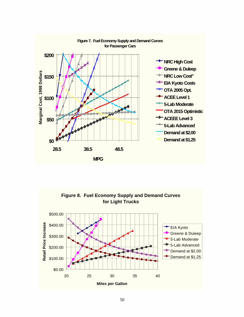
50

Figure 7. Fuel Economy Supply and Demand Curvesfor Passenger Cars

$0

$50

$100

$150

$200

28.5 38.5 48.5

MPG

Mar

gin

al C

ost

, 199

8 D

olla

rs

NRC High Cost

Greene & Duleep

NRC Low Cost"

EIA Kyoto Costs

OTA 2005 Opt.

ACEE Level 1

5-Lab Moderate

OTA 2015 Optimistic

ACEEE Level 3

5-Lab Advanced

Demand at $2.00

Demand at $1.25

Figure 8. Fuel Economy Supply and Demand Curvesfor Light Trucks

$0.00

$100.00

$200.00

$300.00

$400.00

$500.00

20 25 30 35 40

Miles per Gallon

Ret

ail P

rice

Incr

ease EIA Kyoto

Greene & Duleep

5-Lab Moderate

5-Lab Advanced

Demand at $2.00

Demand at $1.25

51

the graph, while those based on the longer-run analyses tend to occupy the lower half of the quadrant. The “5-Lab Study 2015 Advanced Scenario” curve implies almost constant marginal costs for fuel economy improvement. The “NRC High Cost” curve slopes upward very steeply. The highest intercept (cost for the first small mpg improvement, however, belongs to the curve inferred from EIA’s Cost of Kyoto study. The fewer light truck fuel economy supply curves exhibit a similar pattern. Figures 7 and 8 also show hypothetical demand curves for fuel economy, constructed based on typical usage patterns of U.S. household vehicles, a base mpg of 28.5 on the federal test procedure for cars and 20.5 for light trucks (25 and 17.5 mpg, respectively, on the road), an annual discount rate of 10 percent, annual miles traveled by a new vehicle of 15,220 declining at 4.5 percent per year, a 13.7 year average life, and gasoline prices of $1.25 and $2.00, respectively. Levels of incremental fuel economy improvement predicted by the intersection of supply and demand curves for automobiles and based on the near-term studies range from less than 1 mpg for the “NRC High Cost” curve to over 8 mpg for the “ACEEE Level 1” curve. For the longer-term curves, at $1.25 per gallon, hypothetical market fuel economy increases range from 11 to 16 mpg. At $2.00 per gallon, the range of mpg improvements for short-term studies is from just under 2 to just over 11 mpg. The range for longer-term studies is from 16 to 23 mpg. For light trucks, the Greene and Duleep curve implies a hypothetical market solution of a 3 mpg improvement to 23.5 mpg at $1.25 per gallon; 25 mpg at $2.00 per gallon. The 5-Lab Advanced Scenario curve implies a jump to 30 mpg based on the value of fuel savings at $1.25, 34 mpg at $2.00. Each fuel economy supply curve, combined with the two demand curves implies a fuel price elasticity of fuel economy. Credible econometric estimates of U.S. price elasticities for mpg are essentially non-existent due to the effects of the CAFE standards on the market for fuel economy since 1975 (Greene, 1990; 1998). Dahl (1986) reviewed econometric studies done prior to 1985 and found an average, long-run, fuel price elasticity of mpg of +0.57. None of the studies reviewed, however, adequately account for the effects of CAFE standards. Based on an analysis of more recent evidence, Greene (1996) concluded that an elasticity of about +0.2 was more likely to reflect an unregulated market response, but that all available studies had serious shortcomings. The curves presented in Figures 7 and 8 therefore constitute potentially valuable sources of insights about this key parameter. We calculate and tabulate these elasticity estimates below. The fuel price elasticity of fuel economy is strongly dependent on technology. The same fuel price change, from $1.25 to $2.00 gives passenger cars a 1 mpg increase under the NRC High Cost technology assumptions, but a 9.5 mpg increase under the 5-Lab Advanced Scenario technology set. Similarly, the Greene and Duleep supply curve associates a 1.5 mpg increase for light trucks with an increase in gasoline prices from $1.25 to $2.00. The 5-Lab Advanced Scenario curve indicates a 4 mpg gain for the same price change. These results are interesting because they indicate that advances in technology may not only increase the economically efficient level of fuel economy, but increase the price elasticity of fuel economy, as well. Increasing the

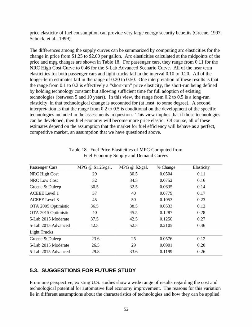
52

price elasticity of fuel consumption can provide very large energy security benefits (Greene, 1997; Schock, et al., 1999) The differences among the supply curves can be summarized by computing arc elasticities for the change in price from $1.25 to $2.00 per gallon. Arc elasticities calculated at the midpoints of the price and mpg changes are shown in Table 18. For passenger cars, they range from 0.11 for the NRC High Cost Curve to 0.46 for the 5-Lab Advanced Scenario Curve. All of the near term elasticities for both passenger cars and light trucks fall in the interval 0.10 to 0.20. All of the longer-term estimates fall in the range of 0.20 to 0.50. One interpretation of these results is that the range from 0.1 to 0.2 is effectively a “short-run” price elasticity, the short-run being defined by holding technology constant but allowing sufficient time for full adoption of existing technologies (between 5 and 10 years). In this view, the range from 0.2 to 0.5 is a long-run elasticity, in that technological change is accounted for (at least, to some degree). A second interpretation is that the range from 0.2 to 0.5 is conditional on the development of the specific technologies included in the assessments in question. This view implies that if those technologies can be developed, then fuel economy will become more price elastic. Of course, all of these estimates depend on the assumption that the market for fuel efficiency will behave as a perfect, competitive market, an assumption that we have questioned above.

Table 18. Fuel Price Elasticities of MPG Computed from Fuel Economy Supply and Demand Curves

Passenger Cars MPG @ $1.25/gal. MPG @ $2/gal. % Change Elasticity

NRC High Cost 29 30.5 0.0504 0.11

NRC Low Cost 32 34.5 0.0752 0.16

Greene & Duleep 30.5 32.5 0.0635 0.14

ACEEE Level 1 37 40 0.0779 0.17

ACEEE Level 3 45 50 0.1053 0.23

OTA 2005 Optimistic 36.5 38.5 0.0533 0.12

OTA 2015 Optimistic 40 45.5 0.1287 0.28

5-Lab 2015 Moderate 37.5 42.5 0.1250 0.27

5-Lab 2015 Advanced 42.5 52.5 0.2105 0.46

Light Trucks

Greene & Duleep 23.6 25 0.0576 0.12

5-Lab 2015 Moderate 26.5 29 0.0901 0.20

5-Lab 2015 Advanced 29.8 33.6 0.1199 0.26

5.3. SUGGESTIONS FOR FUTURE STUDY From one perspective, existing U.S. studies show a wide range of results regarding the cost and technological potential for automotive fuel economy improvement. The reasons for this variation lie in different assumptions about the characteristics of technologies and how they can be applied

53

as well as different methods for estimating technological potential. Without doubt, the greatest source of differences among studies is disagreement about the costs of fuel economy technologies. Additional cost analyses would help, to be sure, but so would more careful adherence to a set of standard assumptions about normal versus accelerated capital turnover, application of overhead costs, and so on. It would be naï ve, however, to expect that in a highly charged policy debate, analysts will refrain from tailoring assumptions to produce results supporting a particular view. The actual process of automotive design is much more integrated than its simple representation in technology/cost analysis, and weighs many more factors than are explicitly addressed in a fuel economy assessment. Outside of the industry—indeed, outside of an actual product development process underway—it is difficult to obtain details about all of these factors and now they are taken into account. The extent to which further study can provide evidence favoring one assumption over another as a way to narrow the range of estimates is unclear. Beyond these considerations, however, there are broad areas in which further research can produce valuable insights about this critical subject of policy analysis. From a broader perspective, nearly all existing studies indicate that some non-trivial degree of fuel economy improvement can be had at modest cost. In terms of providing additional insights valuable for informing the policy debate about fuel economy, it may be more important to investigate several issues that go beyond the technology/cost analysis framework, rather than attempting to sharpen it further. These issues, which are interrelated, include developing better ways to represent: (1) the characteristics, drivers, and effects of innovation in automotive technology; (2) effects of regulation in shaping design decisions and expanding the technology options available; and (3) the role of capital constraints in technology deployment decisions. While the particulars of the automotive design process may be difficult to investigate empirically, further analysis could be done to shed light on the outcome with respect to technology innovations that have occurred recently and historically in the industry. Innovation is a subject of great interest in both business and economics. There has been a perennial debate over the role of government in innovation, with a generally accepted role for government in funding fundamental research, and a more controversial role regarding "technology policy," whether or not government should be involved in fostering development and commercialization of R&D applications. By and large, fuel economy assessments have not drawn on the literature on innovation. It would be valuable to examine the characteristics of past innovation in the automotive industry (whether the innovations were motivated at all or in part by societal concerns) and to see what lessons can be drawn for how to better represent the prospects for and costs of future fuel economy improvements. Secondly, it would be valuable to develop a pragmatic understanding of how regulations shape not only automotive design under a fixed set of options but also the technology development process through which new design options are created. Fundamentally, regulations force the outcome of the design process to address the concerns motivating the policy. They are not the only public policies that influence design; pricing policies can do so indirectly, for example. But given regulation's documented effects (on safety and tailpipe emissions as well as fuel economy),

54

they will remain a key subject of policy analysis, and so any unique attributes of regulations must be thoroughly understood. Although most recent studies of fuel economy potential were at least partially motivated by prospective regulatory initiatives, none of them explicitly address the effects of regulation per se. At this point, the United States has over 30 years of experience with regulation to address some societal concerns about car design. It would be useful to review this history, gather data on specific technologies and design changes related to regulatory concerns, and attempt to understand the influences, not only on aggregate outcomes and performance indicators such as CAFE, but also on the regulated design process itself. It may thereby become possible to develop models useful for analyzing prospective energy and environmental regulations. Finally, another topic for investigation is the implication for automotive product development programs of capital constraints and risk. The industry is highly capital intensive and is self-financing, relying on pubic financial markets. Major investments must be justified by their expected returns. Any given vehicle program competes with others in the company, which itself competes with other companies in the financial markets, for capital resources. Ultimately, these investment resources are constrained by the expected revenue returns from sales, related to the total size of the retail market and the average vehicle price that the market will bear. Under such competitive circumstances, new product budgets are proposed and approved, and so ongoing pressure exists to hold down the time and cost it takes to develop new products. As changing requirements are placed on design (by either market forces or public policy), decisions will be made to spend product development resources on some things and not on others. For example, consider the cost of a requirement to improve fuel economy by a certain amount over a decade's time. Market and capital constraints may limit the average new vehicle price increase to, say, 10 percent over this period of time, and this ceiling may determine the pricing outcome regardless of regulatory requirements. Without regulations, automakers may add $2,000 worth of amenities to vehicles (navigation, entertainment, communications systems; comfort and convenience items, etc.). With regulations, some of this amenity may be foregone, as automakers have to spend some of the $2,000 to add technologies needed to improve efficiency. In general, if expected total returns (sales revenues) are not expanded, then product development resources cannot be increased except at risk to profit. Thus, design trade-offs will be made, and some options that might have been pursued before the change in requirements will not be pursued in favor of those that address the changed conditions. If vehicle prices are limited and therefore development budgets are constrained, the costs of changing requirements may be only the opportunity costs of forgoing design changes that might otherwise have been pursued. The applicability of this view needs to be examined, as well as the extent of such resource constraints and the implications for design and pricing.

55

6. CONCLUSIONS Technology/cost analysis has emerged as the method of choice for policy analyses of the potential for fuel economy improvement. The blueprint it provides, illustrating how higher levels of fuel economy can be achieved at a given cost, provides a proof of feasibility and practicality that is critically important to policy debates. Holding other vehicle attributes constant so that the trade-off between fuel economy and cost is clearly defined, has proven to be a valuable assumption for policy analysis, both because it is intuitive and because it allows for clear interpretation of costs (it also facilitates construction of supply curves which have additional analytical value). The constant other attributes assumption is less valuable in the context of forecasting, because real-world markets are likely to trade-off fuel economy for other attributes of interest to the consumer. The important distinction between these two kinds of technology/cost analysis, those that hold other vehicle characteristics constant and strictly describe the fuel economy versus cost trade-off and those that attempt to simulate the behavior of real markets, is often overlooked. Historically, differences in assumptions and conventions across analyses have lead to widely divergent conclusions across studies. To a limited degree, additional research can help resolve some of these differences. The largest area of disagreement about data is clearly the costs of fuel economy technologies. Here, focused research on the costs of specific technologies would help to narrow the gaps. Greater clarity in documenting assumptions about technology impacts and costs would also be helpful. Nonetheless, analysts will continue to hold different opinions, and the nature of policy debates will always produce analyses with differing conclusions about the costs of fuel economy improvement. Nearly every technology cost analysis ever done, regardless of by whom or for what purpose has demonstrated at least some small potential to cost-effectively increase fuel economy beyond current market levels. Recent studies limited to proven technologies and considering a time horizon of about 10 years suggest passenger car fuel economy improvement potentials to the range of 32 to 41 mpg, at costs in the vicinity of $750 per car. Longer-term analyses considering the possibility of technological change suggest technology potentials to the range of 38 to 52 mpg, at costs below $1,000 per car. Given additional assumptions, these fuel economy potential and cost estimates can be used to estimate the elasticity of new car fuel economy with respect to fuel price. The near-term, proven technology analyses imply elasticities in the range of 0.10 to 0.20. The longer-term analyses, which incorporate new and as yet unproven technologies, imply elasticities about twice as great, reflecting an elasticity-enhancing effect of technological progress. These elasticities reflect only technology and design changes and not changes in the mix of vehicles sold. The growing interest in longer-term policy issues, such as greenhouse gas emissions, has pushed technology/cost analyses to more fully consider how technological change will influence future fuel economy potentials. This is a relatively new area of analysis, with little in the way of formal methodology on which to draw. To date, the most common approach to dealing with the uncertainties inherent in such assessments is to construct several alternative scenarios. Methods

56

for predicting the impacts of policies, such as regulatory standards or investments in R&D, on the rates and directions of technological changes are virtually non-existent. In addition to the need to continually update and refine estimates based on established methods, these questions raised by longer-term policy issues offer ample challenges for energy policy researchers in the years ahead.

57

7. REFERENCES

1. Adler, P. and K. Clark. (1991). “Behind the Learning Curve: A Sketch of the Learning Process”, Management Science, vol. 37, pp. 267-281.

2. Arrow, K.J., W.R. Cline, K.-G. Maler, M. Munasinghe, R. Squitieri and J.E. Stiglitz.

(1995). “Intertemporal Equity, Discounting, and Economic Efficiency,” Ch. 4 in, Climate Change 1995: Economic and Social Dimensions of Climate Change, J.P. Bruce, H. Lee and E.F. Haites, eds., published for the Intergovernmental Panel on Climate Change by Cambridge University Press.

3. Associated Press. (1988). “Japanese Car Sets Record at 6,409 mpg,” Knoxville News

Sentinel, July 3, Business/Automotive Section, p. 7.

4. Berger, J.O., M.H. Smith, and R.W. Andrews. (1990a). “A System for Estimating Fuel Economy Potential Due to Technology Improvements,”research report for Ford Motor Company, Purdue University, Indiana, November 5.

5. Berger, J.O., M.H. Smith, and R.W. Andrews. (1990b). “Combined Estimation of the

Fuel Economy Potential due to Technology Improvements,” Presented at the SAE Government/Industry Meeting, Washington, DC, May.

6. Bleviss, D. (1988). The New Oil Crisis and Fuel Economy Technologies: Preparing the

Light Transportation Industry for the 1990s. New York : Quorum Books.

7. Burke, M.S. (1992). Optimizing product Development Life Cycles in the U.S. Auto Industry, M.S. Thesis, Department of Mechanical Engineering and School of Management, Cambridge, MA: Massachusetts Institute of Technology, June.

8. Clark, K.B., and T. Fujimoto. (1991). Product Development Performance: Strategy,

Organization, and Management in the World Auto Industry, Boston, MA : Harvard Business School Press.

9. Congress of the United States, Congressional Budget Office. (1980). Fuel Economy

Standards for New Passenger Cars After 1985, U.S. Government Printing Office, Washington, DC, December.

10. Cornille, H.J., J.C. Weishaar, and C.S. Young. (1998). The P2000 Body Structure, SAE

Technical Paper No. 982405, Warrendale, Pennsylvania : Society of Automotive Engineers.

11. Coon, C.W., B.C. Dial, R. Hemion, R.W. Hull, R.J. Mathis, C. Morrison, L. Rhymes,

C.D. Wood, S.W. Seale, T. Stettler, C. Rech, H.O. Woller and J.W. Colburn, Jr. (1974). Technological Improvements to Automobile Fuel Consumption, Final Report, Vol. II,

58

prepared for the U.S. Department of Transportation, Office of the Secretary, Washington, DC and the U.S. Environmental Protection Agency, Ann Arbor, Michigan, December.

12. Curran, H.M., W.R. Menchen, T.V. Bolan and K.R. Hall. (1976). Fuel Economy/Cost

Relationships for Future Automobiles, HIT-637, Hittman Associates, Inc., Columbia Maryland, January.

13. Dahl, C.A. (1986). “Gasoline Demand Survey,” The Energy Journal, vol. 7, no. 1, pp.

67-82.

14. DeCicco, J.M. (1997). Developing a Market Creation Program to Promote Efficient Cars and Light Trucks, Washington, DC : American Council for an Energy-Efficient Economy. August.

15. DeCicco, J.M., and M. Ross. (1996). “Recent Advances in Automotive Technology and

the Cost-Effectiveness of Fuel Economy Improvement,” Transportation Research, 1D(2): 79-96.

16. DeCicco, J.M. and M. Ross. (1993). An Updated Assessment of the Near-Term

Potential for Improving Automotive Fuel Economy, Washington, DC: American Council for an Energy-Efficient Economy, November.

17. Difiglio, C., K.G. Duleep, and D.L. Greene. (1990). “Cost Effectiveness of Future Fuel

Economy Improvements,” Energy Journal, 11(1):65-68, January.

18. Duleep, K.G. (1997). “The Potential for Evolutionary and Revolutionary Technologies to Improve Automotive Fuel Economy,”Chapter 7 in J. DeCicco and M. Delucchi (eds.), Transportation, Energy, and the Environment: How Far Can Technology Take Us? Washington, DC: American Council for an Energy-Efficient Economy.

19. Energy and Environmental Analysis, Inc. (1991). Documentation of Attributes of

Technologies to Improve Automotive Fuel Economy, report prepared for the U.S. Department of Energy, Arlington, Virginia, October.

20. Energy and Environmental Analysis, Inc. (1990a). Analysis of the Fuel Economy

Boundary for 2010 and Comparison to Prototypes, report prepared for the U.S. Department of Energy, Arlington, Virginia, November.

21. Energy and Environmental Analysis, Inc. (1990b). An Assessment of Potential Passenger

Car Fuel Economy Objectives for 2010, Arlington, Virginia, June.

22. Energy and Environmental Analysis, Inc. (1988). Light Duty Truck Fuel Economy Review and Projections 1980—1995, Final Report,” DOE/OR/21400-HO, Office of Policy, Planning and Analysis, U.S. Department of Energy, Washington, DC, November.

59

23. Energy and Environmental Analysis, Inc. (1986). Analysis of the Capabilities of Domestic Auto-Manufacturers to Improve Corporate Average Fuel Economy, DOE/RL/01830-H1, Office of Policy, Planning and Analysis, U.S. Department of Energy, Washington, DC.

24. Energy and Environmental Analysis, Inc. (1985). Documentation of the Characteristics

of Technological Improvements Utilized in the TCSM, report prepared for the U.S. Department of Energy, Arlington, VA: June.

25. Energy and Environmental Analysis, Inc. (1981). The Technology/Cost Segment Model

Post-1985 Automotive Fuel Economy Analysis Final Report, prepared for the Office of Conservation, U.S. Department of Energy, Arlington, Virginia: November.

26. Energy and Environmental Analysis, Inc. (1979). Technological/Cost Relations to

Update DOE/Faucett Model, report to the U.S. Department of Energy, Washington, DC, Arlington, VA: October.

27. FCTAP. (1998). Status and Prospects of Fuel Cells as Automobile Engines, report of

the Fuel Cell Technical Advisory Panel, Sacramento, California : California Air Resources Board, July.

28. Ford, A. (1984). “Uncertainty in the Price of Gasoline and the Automobile

Manufacturers’ 1990 Retooling Decision,” Energy, vol. 9, no. 6, pp. 519-540.

29. Ford, A. and R.J. Sutherland. (1982). The Outlook for Improved Automobile Fuel Efficiency, LA-9414-MS, UC-98, Los Alamos National Laboratory, Los Alamos, New Mexico, June.

30. Gray, C.L. and F. von Hippel. (1981). “The Fuel Economy of Light Vehicles,” Scientific

American, vol. 244, no. 5, pp. 48-59.

31. Greene, D.L. (1998). “Why CAFE Worked,” Energy Policy, vol. 26, no. 8, pp. 595-614.

32. Greene, D.L. (1997). “Oil Dependence: The Value of R&D,” pp. 2148-2153 in, IECEC-97: Proceedings of the Thirty-Second Intersociety Energy Conversion Engineering Conference, Vol. 3, July27-Aug. 1, Honolulu, Hawaii, American Institute of Chemical Engineers, New York, NY.

33. Greene, D.L. (1996). “Transportation,” Chapter 5 in Policies and Measures for

Reducing Energy-Related Greenhouse Gas Emissions, DOE/PO-0047, Office of Policy and International Affairs, U.S. Department of Energy, Washington, DC, July.

34. Greene, D.L. (1990). “CAFE OR PRICE? An Analysis of the Effects of Federal Fuel

Economy Regulations and Gasoline Price on New Car MPG,” The Energy Journal, vol. 11, no. 3, pp. 37-57.

60

35. Greene, D.L. and K.G. Duleep. (1993). “Costs and Benefits of Automotive Fuel Economy Improvement: A Partial Analysis,” Transportation Research 27A(3): 217-235.

36. Greene, D.L. and K.G. Duleep. (1992). Costs and Benefits of Automotive Fuel Economy

Improvement: A Partial Analysis, ORNL-6704, Oak Ridge, TN: Oak Ridge National Laboratory, Center for Transportation Analysis, March.

37. Heavenrich, Robert M. and Karl H. Hellman. (1996). Light-Duty Automotive Technology

and Fuel Economy Trends through 1996, EPA/AA/TDSG/96-01, Ann Arbor, MI: U.S. Environmental Protection Agency, Office of Mobile Sources, August.

38. Hittman Associates, Inc. (1976). Fuel Economy/Cost Relationships For Future

Automobiles, JACKFAU 76-137-5, Final Report to the Federal Energy Administration, January, Columbia, Maryland.

39. Ingrassia, P., and J.B. White. (1994). Comeback: The Fall and Rise of the American

Automobile Industry, New York: Simon & Schuster.

40. Interlaboratory Working Group. (1997). Scenarios of U.S. Carbon Reductions Potential Impacts of Energy Technologies by 2010 and Beyond, LBNL—40533, Lawrence Berkeley National Laboratory, Berkeley, California, September.

41. Keebler, J. (1991). “Runkle Urges ‘Moon Shot’ on Energy, Air and Safety,” Automotive

News, January 21, p. 1.

42. Kelly, H. and R.H. Williams. (1992). “Fuel Cells and the Future of the U.S. Automobile,” working paper, Princeton University, Center for Energy and Environmental Studies, December.

43. Ledbetter, M., and M. Ross. (1990). “Supply Curves of Conserved Energy for

Automobiles,” Proceedings of the 25th Intersociety Energy Conversion Engineering Conference, Reno, NV, August.

44. Lovins, A. (1995). “Hypercars: The Next Industrial Revolution,” Chapter 5 in D.

Sperling and S.A. Shaheen (eds.), Transportation and Energy: Strategies for a Sustainable Transportation System, Washington, DC: American Council for an Energy-Efficient Economy.

45. Lovins, A.B., J.W. Barnett and L.H. Lovins. (1993). “Supercars: The Coming Light-

Vehicle Revolution,” presented at the 1993 Summer Study of the European Council for an Energy Efficient Economy, RungstedgDrd, Denmark, June 1-5, published by the Rocky Mountain Institute, Smowmass, Colorado.

46. Menchen, W.R., H.A. Curran, B.K. Hinkle, C.L. Jedlicka, J.E. Reed, J.P. Overman.

(1974). A Study of Industry Response to Policy Measures Designed to Improve

61

Automobile Fuel Economy, HIT-571, Hittman Associates, Inc., Final Report to the Council on Environmental Quality, contract no. EQ4AC006, Washington, DC.

47. Murrell, J.D. (1990). How Fuel Economy Responds to Changes in Weight, CID, and

N/v, Ann Arbor, MI: U.S. Environmental Protection Agency, Office of Mobile Sources.

48. OSAT. (1998). Delphi IX: Forecast and Analysis of the North American Automotive Industry. Executive Summary, Ann Arbor, MI: University of Michigan Transportation Research Institute, Office for the Study of Automotive Transportation.

49. National Research Council, Standing Committee to Review the Research Program of the

Partnership for a New Generation of Vehicles. (1999). Review of the Partnership for a New Generation of Vehicles: Fifth Report, National Academy Press, Washington, DC.

50. NRC. (1992). Automotive Fuel Economy: How Far Should We Go? Report of the

National Research Council, Committee on Fuel Economy of Automobiles and Light Trucks. Washington, DC: National Academy Press.

51. Ogden, J.M., M.M. Steinbugler and T.G. Kreutz. (1999). “A Comparison of Hydrogen,

Methanol, and Gasoline as Fuels for Fuel Cell Vehicles: Implications for Vehicle Design and Infrastructure Development,” Journal of Power Sources, vol. 79, pp. 143-168.

52. Ross, M. (1994). “Automobile Fuel Consumption and Emissions: Effects of Vehicle and

Driving Characteristics,” Annual Review of Energy and Environment, Vol. 19.

53. Schock, R.N., W. Fulkerson, M.L. Brown, R.L. San Martin, D.L. Greene and J. Edmonds. (1999). How Much is Energy R&D Worth as Insurance? UCRL-JC-131205, Lawrence Livermore National Laboratory, Livermore, California, March.

54. Sovran, G. (1983). Tractive-Energy-Based Formulae for the Impact of Aerodynamics on

Fuel Economy Over the EPA Driving Cycle, SAE Technical Paper 830304, Society of Automotive Engineers, Warrendale, PA.

55. Sovran, G., and M.S. Bohn. (1981). Formulae for the Tractive-Energy Requirements of

Vehicles Driving the EPA Schedules, SAE Paper 810184, Society of Automotive Engineers, Warrendale, PA.

56. Shackson, R.H. and H.J. Leach. (1980). Maintaining Automotive Mobility: Using Fuel

Economy and Synthetic Fuels to Compete With OPEC Oil, The Energy Productivity Center, Mellon Institute, Arlington, Virginia.

57. Stephenson, R.R. (1975). Should We Have a New Engine? JPL SP 43-17, vol. I, Jet

Propulsion Laboratory, California Institute of Technology, Pasadena, California.

62

58. Stobart, R.K. (1999). Fuel Cell Power for Passenger Cars—What Barriers Remain? SAE Paper No. 1999-01-0321, Warrendale, Pennsylvania, Society of Automotive Engineers.

59. U.S. Congress, Office of Technology Assessment. (1995). Advanced Automotive

Technology: Visions of a Super-Efficient Family Car, OTA-ETI-638, U.S. Government Printing Office, Washington, DC, September.

60. U.S. Congress, Office of Technology Assessment. (1991). Improving Automobile Fuel

Economy: New Standards, New Approaches, OTA-E-504, U.S. Government Printing Office, Washington, DC.

61. U.S. Congress, Office of Technology Assessment. (1982). Increased Automobile Fuel

Efficiency and Synthetic Fuels: Alternatives for Reducing Oil Imports, U.S. Government Printing Office, Washington, DC, September.

62. U.S. Department of Energy, Energy Information Administration. (1998). Impacts of the

Kyoto Protocol on U.S. Energy Markets and Economic Activity, SR/OIAF/98-03, Washington, DC, October.

63. U.S. Department of Energy, Energy Information Administration. (1994). Model

Documentation Report: Transportation Sector Model of the National Energy Modeling System, DOE/EIA-M070, Washington, DC, March.

64. U.S. Department of Transportation, National Highway Traffic Safety Administration.

(1978). Rulemaking Support Paper - Supplement for the Light Truck and Van Fuel Economy Standards for Model Years 1980 and 1981, Washington, DC, May.

65. U.S. Department of Transportation, National Highway Traffic Safety Administration.

(1977a). “Passenger Automobile Average Fuel Economy Standards: Final Rule,” Federal Register, vol. 42, no. 126, Thursday, June 30, 1977, Part VII, pp. 33534-33552, Washington, DC.

66. U.S. Department of Transportation, National Highway Traffic Safety Administration.

(1977b). Data and Analysis for 1981-1984 Passenger Automobile Fuel Economy Standards: Summary Report, Office of Automotive Fuel Economy, Washington, DC, February 28.

67. U.S. Department of Transportation, U.S. Environmental Protection Agency. (1975a).

“Study of Potential for Motor Vehicle Fuel Economy Improvement,” Report #5, Economics Panel Report, January 10, Washington, DC.

68. U.S. Department of Transportation, U.S. Environmental Protection Agency. (1975b).

“Study of Potential for Motor Vehicle Fuel Economy Improvement,” Report #4, Technology Panel Report, January 10, Washington, DC.

63

69. Varian, H.R. (1992). Microeconomic Analysis, third edition, W.W. Norton & Co., New

York.

70. Werbos, P. (1987). Oil Dependency and the Potential for Fuel Cell Vehicles, SAE Paper No. 871091, Warrendale, Pennsylvania, Society of Automotive Engineers.

71. Whitford, R.K. (1984). “Fuel Efficient Autos: Progress and Prognosis,” Annual Review

of Energy, vol. 9, pp. 375-408.

72. Womack, J.P., D.T. Jones, and D. Roos. (1990). The Machine that Changed the World, New York: Rawson Associates.

64

65

APPENDIX APPROXIMATION OF TOTAL COST CURVES BY QUADRATIC FUNCTIONS We approximate each study=s total cost function for fuel economy improvement by means of quadratic curves. There are three reasons for choosing the quadratic function:

1. A quadratic curve with intercept equal to zero is a second order power series approximation to any arbitrary function in the vicinity of the origin. By construction, total cost curves must have positive first derivatives and second derivatives that are $0. The quadratic curve is the lowest order polynomial that can have both of these properties. By defining the x-axis zero point as the current fuel economy level, we know that the curve will pass through the origin, since the cost of no increase in fuel economy must be zero. Thus, only two parameters need to be estimated to define each curve.

2. For those studies that explicitly provide points on a total cost curve, the quadratic function appears to provide a good fit to the data.

3. A linear marginal cost (supply) curve for fuel economy can be easily derived from the quadratic total cost curve.

Of course, there is no a priori reason why the total cost curve must be quadratic. It is used here as a simple and appropriate approximation. Calibration Methods Least Squares Fitting. If studies provide three or more data points, curves can be fitted by least squares methods. With less than ten data points, this is merely a curve fitting exercise, without statistical significance. Exact Fit to Two Points. A quadratic curve is defined by three points. Thus, only two non-zero points are required to define a total cost curve for fuel economy improvement. Let total cost, C, be a function of the improvement in fuel economy over a base level, MPG-MPG0 = ∆MPG = X.

( )C X a a X a Xo

= + +1 2

2

Since, by construction, C(0) = 0, it is always true that a0 = 0. Given two points, (C(X1), X1) and (C(X2), X2) , we construct two linear, simultaneous equations that are readily solved for the two unknowns, a1 , and a2 .

66

Calibration to One Point and Marginal Cost = Marginal Utility. A quadratic can even be fitted to two or more MPG forecasts, provided that, (1) the forecast may be assumed to represent a competitive market equilibrium solution, (2) the price of fuel at a point is known, and (3) other reasonable assumptions can be made about vehicle use and discount rates. The method depends on the fact that at any given point, the marginal cost (MC) of further fuel economy improvement (which is the slope of the total cost curve) equals the marginal value (MV) of the fuel savings.7 Knowing the slope of the total cost curve at two points, gives the two pieces of data necessary to estimate the two parameters of the quadratic curve. The equations are shown below.

MC b CX

MC b CX1 1

2 2

2

2

= += +

MC is calculated by computing the value of a 1 MPG increase at the point X1 . The 1 MPG increment is centered at X by computing the increase from X1 - 2 to X1 + 2 . The inaccuracy inevitably introduced by the assumptions necessary to compute the discounted present value of fuel savings due to the 1 MPG increase can be minimized by matching them as closely as possible to the assumptions used to make the forecast. If n points are given, then the number of possible curves that can be computed is n!/(2!(n-2)!). If these curves are very different, it implies that either, (1) the underlying cost curve is not quadratic, or (2) the assumption that the forecast represents a perfect market equilibrium is incorrect. All three methods were used in computing the quadratic total cost curves presented in this report. The ACEEE and NRC cost curves were computed by least squares fitting. The OTA cost curves was computed from two points, and the EIA Kyoto and 5-Lab Study curves were computed using the MC method. The differences in method undoubtedly introduce some incomparabilities among the curves. This is perhaps best illustrated by the apparent lack of curvature in the EIA cost curves. This is very likely an artifact of the method, which imposes a cost curve concept on the dynamic NEMS model. Nonetheless, the relative positions of the curves and approximate slopes remain indicative of the underlying cost-MPG relationship inherent in the different analyses. APPARENT DISCOUNTING OF FUTURE FUEL SAVINGS The relationship between the discount rates appropriate for investments in depreciating versus non-depreciating assets can be illustrated by a mathematical example. Suppose that a capital investment has an initial cost of K and is held for a period of T years. If the market rate of interest (reflecting the opportunity cost of capital) is r, and if we discount at rate r, then the sum of the discounted stream of interest payments plus the discounted value of the non-depreciated capital T years from the present exactly equals K. Assuming that the market rate of interest and discount rate are equal implies that markets are allocating investments efficiently over time.

7The assumption that markets are in equilibrium is a strong one, as is the assumption that other

factors

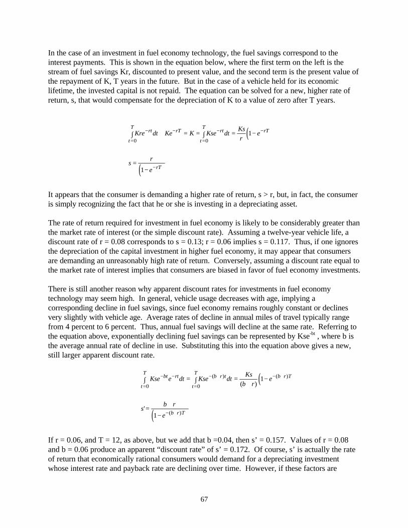
67

In the case of an investment in fuel economy technology, the fuel savings correspond to the interest payments. This is shown in the equation below, where the first term on the left is the stream of fuel savings Kr, discounted to present value, and the second term is the present value of the repayment of K, T years in the future. But in the case of a vehicle held for its economic lifetime, the invested capital is not repaid. The equation can be solved for a new, higher rate of return, s, that would compensate for the depreciation of K to a value of zero after T years.

( )

( )

Kre dt Ke K Kse dtKs

re

sr

e

rt rT

t

Trt

t

TrT

rT

− −

=

−

=

−

−

+ = =∫ ∫ = −

=−

0 01

1

It appears that the consumer is demanding a higher rate of return, s > r, but, in fact, the consumer is simply recognizing the fact that he or she is investing in a depreciating asset. The rate of return required for investment in fuel economy is likely to be considerably greater than the market rate of interest (or the simple discount rate). Assuming a twelve-year vehicle life, a discount rate of r = 0.08 corresponds to s = 0.13; r = 0.06 implies s = 0.117. Thus, if one ignores the depreciation of the capital investment in higher fuel economy, it may appear that consumers are demanding an unreasonably high rate of return. Conversely, assuming a discount rate equal to the market rate of interest implies that consumers are biased in favor of fuel economy investments. There is still another reason why apparent discount rates for investments in fuel economy technology may seem high. In general, vehicle usage decreases with age, implying a corresponding decline in fuel savings, since fuel economy remains roughly constant or declines very slightly with vehicle age. Average rates of decline in annual miles of travel typically range from 4 percent to 6 percent. Thus, annual fuel savings will decline at the same rate. Referring to the equation above, exponentially declining fuel savings can be represented by Kse-bt , where b is the average annual rate of decline in use. Substituting this into the equation above gives a new, still larger apparent discount rate.

( )

( )

Kse e dt Kse dtKs

b re

sb r

e

bt rt b r t

t

Tb r T

t

T

b r T

− − − +

=

− +

=

− +

= ∫ =+

−∫

=+

−

( ) ( )

( )

( )

'

001

1

If r = 0.06, and T = 12, as above, but we add that b =0.04, then s’ = 0.157. Values of r = 0.08 and b = 0.06 produce an apparent “discount rate” of s’ = 0.172. Of course, s’ is actually the rate of return that economically rational consumers would demand for a depreciating investment whose interest rate and payback rate are declining over time. However, if these factors are

68

overlooked, it appears that consumers are using unreasonably high discount rates when evaluating expenditures on fuel economy technologies. An additional complication is introduced by the fact that new car buyers rarely hold a vehicle for its full economic life. If used car markets perfectly assess the value of remaining fuel savings, and if used car buyers use the same discount rates as new car buyers, the above analysis is unchanged. If, on the other hand, used car markets underestimate the value of future fuel savings or if used car buyers use a higher discount rate, it is easy to show that economically rational new car buyers would demand a still higher rate of return to investments in fuel economy.