Contents lists available at ScienceDirect

Engineering Analysis with Boundary Elements

journal homepage: www.elsevier.com/locate/enganabound

Freeze-drying modeling of vial using BEM

M. Ramšak, J. Ravnik, M. Zadravec, M. Hriberšek, J. Iljaž⁎

Faculty of Mechanical Engineering, University of Maribor, Smetanova 17, SI-2000 Maribor, Slovenia

A R T I C L E I N F O

Keywords:Freeze-dryingVialHeat and mass transferSubdomain boundary element methodSublimation

A B S T R A C T

The paper reports on development of Boundary Element Method (BEM) based numerical algorithm for thenumerical simulation of the freeze drying process in a vial. In the paper the problems of freeze-drying modelingare covered in detail. The BEM based algorithm is developed for the axisymmetrical geometry case using theSubdomain BEM approach. A special feature of the algorithm is an implicit representation of the interfaceconditions at the sublimation front, which is a great advantage of the proposed numerical scheme. As a test casethe freeze drying of skim milk in a vial is selected. The numerical results show a good agreement with referencedata proving that the developed numerical model is appropriate, accurate and fast in simulating the primary andsecondary drying stage. The numerical analysis also shows that the time step during the secondary drying stagecan be increased by a factor 100, which reduces the computational time drastically.

1. Introduction

Freeze-drying or lyophilization is a process of removing the liquidphase, usually water, from the initial wet compound or solution andcan be divided into three stages. The first stage is freezing of the basecompound to solidify it, then the surrounding pressure is lowered tothe level where the frozen water can sublimate and the second stagebegins represented by the sublimation process of the frozen water(primary drying). After the sublimation process ends the third stagebegins that is described by the desorption of the bounded water in thedried material (secondary drying). Because the freeze-drying process iscontrolled at relatively low temperatures, the base material is preservedwith all its quality and also becomes more stable [1]. For this reason,the freeze-drying process is mostly used in the food, chemical,pharmaceutical and biotechnological industry [2–4,1]. In the foodindustry the product is usually placed freely on the trays, where in thepharmaceutical industry the product (solution) is predominantly filledin vials.

The freeze-drying is due to the slow drying rate and high invest-ment cost into the equipment and product batch, a very expensiveprocess. Therefore it needs a careful process planning and control, withthe aim to reduce the drying time and to be as energy efficient aspossible [2,5–7,4,8–10]. To be able to predict the correct drying timesand to set the correct process control so the temperature of the frozensolution or material does not exceed the melting or scorch temperatureduring the drying process, a good mathematical or numerical model isneeded.

Numerical modeling of freeze-drying process is very demandingbecause of the needed knowledge of the heat and mass transferincluding the phase change of liquid (water). The general numericalmodel can be used to describe the freeze-drying process in manysystems, like vials that are very popular in the pharmaceutical industry.However, the freeze-drying process has many characteristics that hadto be included into the numerical model for successful simulation. Thefirst characteristic is that the freeze-drying process is a time dependentproblem, because of the moving sublimation front and changingparameter values of the process. The heat and mass transfer isgoverned by the conservation laws of mass, momentum and energy.The sublimation process at the moving sublimation interface betweenthe frozen and dried region has to be included as well as the desorptionof the bounded water in the dried region. The second characteristic isthat the ratio of heat transfer by conduction, convection and radiationat freeze-drying in vials is very different from the ratio of dryingprocess at the atmospheric conditions, because of the much lowersurrounding pressure, which almost eliminates the convection.Therefore, the conduction and the radiation plays a major role in theheat transfer process [7,5,2]. The next characteristic is that the driedmaterial is highly porous, which can not be described directly due tothe complex internal structure. Therefore, the dry material had to bemodeled using the porous model approach. The freeze-drying processand also the mass transfer of the liquid phase take place at very lowstatic pressure, where the free range between the molecules is verylarge and consequently also the Knudsen number, which questions thecorrectness of using the governing equations that are written for the

http://dx.doi.org/10.1016/j.enganabound.2017.01.011Received 16 November 2016; Received in revised form 26 January 2017; Accepted 30 January 2017

⁎ Corresponding author.E-mail address: jurij.iljaz@um.si (J. Iljaž).

Engineering Analysis with Boundary Elements 77 (2017) 145–156

0955-7997/ © 2017 Elsevier Ltd. All rights reserved.

MARK

continuum phase. This is especially problematic for modeling of themomentum transfer and condensation of the liquid phase (water) inthe lyophilizator chamber and condenser [11,12].

For these reasons, the numerical modeling of freeze-drying processin general is a very demanding task to do, and the accuracy ofcomputational models depend on the used mathematical model.However, to be able to simulate freeze-drying process in the wholelyophilizator, we first need to successfully model and solve the problemof product freeze-drying, what is the main focus of the reported workhere. Through the years, several different mathematical modelsdescribing heat and mass transfer in the freeze-drying process havebeen proposed. From the most simple ones [5] to the advanced modelsusing partial differential equations (PDE) [13–15]. The “sorption-sublimation” model described in [14–18] has proven to be accurateand successful in simulating the freeze-drying process in vial solution.Mascarenhas et al. [17] solved the freeze-drying model using FiniteElement Method (FEM) with arbitrary Lagrangian-Eulerian (ALE)scheme. They applied the 2D axisymmetrical model to the freeze-drying problem in a vial for protein Bovine Somatotropin (BST)and skim milk, where the latter problem has been treated as a 1Dproblem. Sheehan and Liapis [2] upgraded the problem descriptionwith more accurate boundary conditions where they included theradiation and solved the model using the Finite Difference method(FDM). They applied their numerical model to the freeze-drying ofskim milk in vials and investigated three different cases, by changingvial at different locations (center or corner) and setting differentprocess controls for not exceeding the melting and scorch temperature.Recently Song et al. [19,18] and Nam and Song [20] used theFinite Volume Method (FVM) to solve the mathematical modeldescribed by Sheehan and Liapis [2] to solve problem of skim milkfreeze-drying in vial. Since Boundary Element Method solves theintegral representation of the governing equations by using specialweighting functions and simultaneously solve the resulting systemof equations for the function and its derivative, this paper reports onthe novel implementation of the Boundary Element Method (BEM)for the numerical solution of the “sorption-sublimation” model offreeze-drying in vial.

As stated, the paper is focused on the development of numericalmodel for freeze-drying simulation of skim milk in one vial using BEMto solve the complex system of non-linear governing equations in spaceand time domain. The used BEM approach has been already success-fully implemented to various numerical problems from fluid dynamics[21–24], moisture transport [25], bioheat problems [26,27], as well asthe solid-liquid phase change problems [28–30].

The paper is organized as follows. Section 2 describes the freeze-drying in a vial in more detail especially the heat and mass transferphenomena. The derived governing equations (mathematical model)with the description are reported in Section 3. The Section 4 coversthe description of the implemented BEM with fundamental solutionand numerical discretization of governing equations, yielding thecomplete numerical model for freeze-drying simulation in vials.Computational example with validation, results and discussion ispresented in Section 5. The paper ends with the conclusion andacknowledgment in Section 6 and 7, respectively.

2. Freeze-drying in a vial

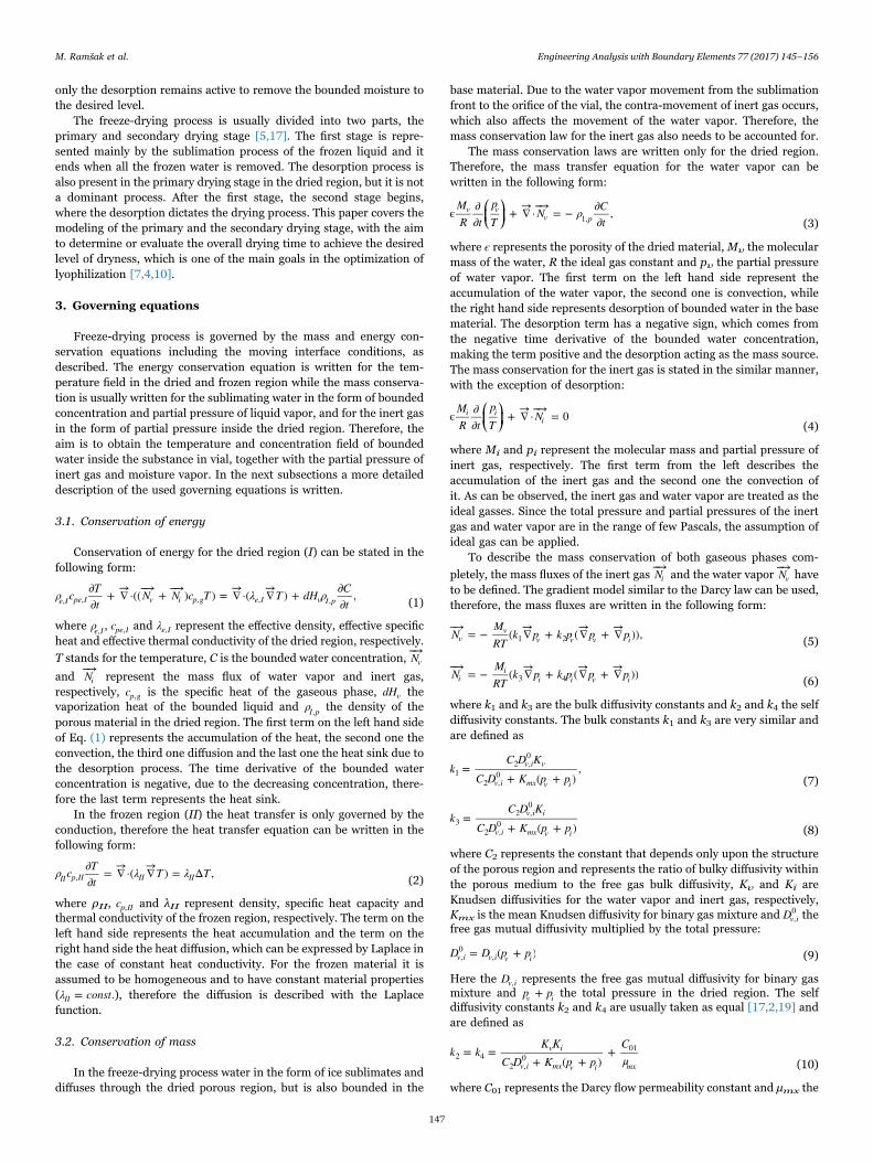
The case under consideration is the freeze-drying stage in vial,which is typically placed on the tray inside a lyophilizator dryingchamber. The vial which contains a drying substance is schematicallyshown on Fig. 1, where three main areas can be observed:

• the area above the initial free surface of the drying substance,consisting of vacuum and evaporated solvent (water vapor),

• the porous region above the sublimation interface, consisting ofsolid matrix with adsorbed solvent,

• the porous region below the sublimation interface, consisting offrozen solvent and solid matrix with adsorbed solvent.

The process starts when the frozen substance is subjected to a suddendecrease in pressure, setting the thermodynamic conditions below thetriple point of the water for sublimation to occur. The freeze-dryingprocess proceeds as follows. The vial is heated by the two heatingplates, one above and one below the vial. The heat is transferred to thefrozen substance from the top, the bottom and through the sides of thevial, as shown in Fig. 1. At the top, the heat transfer is mainly due to theradiation, as the vial is not in the direct contact with the upper plateand the low static pressure of the surrounding decreases conductionand convection heat transfer in the vacuum. The heat from belowcomes from heat radiation and conduction, because of the directcontact between the vial and the lower heating plate. The effect ofthe heat radiation to the side surface of the vial in general depends onthe number and position of the surrounding vials [8], but is frequentlyneglected, especially in the case of fully packed tray in a standardlyophilizator. Here we can conclude that the main contribution of thevial heating comes from above and below. For these reasons, also manyother authors neglect the side heat flux and treat the problem as one-dimensional [5,13,16,17].

The pressure difference between the sublimation surface and thevacuum induces sublimation, which is due to the sublimation enthaplya very energy demanding process. Heating of the shelves solves theproblem of energy supply and enables to take control of the process.Because of the opened top of the vial, the drying starts at the top andproceeds toward the bottom of the vial. On the sublimation front orinterface, which separates the frozen and already dried region, weassume that the concentration or partial pressure of the water is equalto the equilibrium concentration at the interface temperature, and thatthe mass flux of the inert gas is equal to zero, which means that thegradient of partial pressure of the inert gas is also equal to zero. Inaddition, we predict that the temperature on the sublimation front iscontinuous, while the gradient of the temperature is not, because of thesublimation process, as well as of different thermal conductivity of bothregions. The energy conservation law on the interface is described indetail by the used model presented in the next section, here we wouldlike to state only that the net heat flux at the interface also depends onthe movement or velocity of the interface. As stated before, the driedregion is highly porous, therefore, we can presume that there is noclosed pockets and that the inert gas and water vapor can move freely.The movement of gaseous phase in the porous material can bedescribed by the Darcy law. While the sublimation takes place at theinterface, the desorption process from the remaining porous solid isalso present in the dried region. When all the frozen water is removed

Fig. 1. Basic data on freeze drying in a vial.

M. Ramšak et al. Engineering Analysis with Boundary Elements 77 (2017) 145–156

146

only the desorption remains active to remove the bounded moisture tothe desired level.

The freeze-drying process is usually divided into two parts, theprimary and secondary drying stage [5,17]. The first stage is repre-sented mainly by the sublimation process of the frozen liquid and itends when all the frozen water is removed. The desorption process isalso present in the primary drying stage in the dried region, but it is nota dominant process. After the first stage, the second stage begins,where the desorption dictates the drying process. This paper covers themodeling of the primary and the secondary drying stage, with the aimto determine or evaluate the overall drying time to achieve the desiredlevel of dryness, which is one of the main goals in the optimization oflyophilization [7,4,10].

3. Governing equations

Freeze-drying process is governed by the mass and energy con-servation equations including the moving interface conditions, asdescribed. The energy conservation equation is written for the tem-perature field in the dried and frozen region while the mass conserva-tion is usually written for the sublimating water in the form of boundedconcentration and partial pressure of liquid vapor, and for the inert gasin the form of partial pressure inside the dried region. Therefore, theaim is to obtain the temperature and concentration field of boundedwater inside the substance in vial, together with the partial pressure ofinert gas and moisture vapor. In the next subsections a more detaileddescription of the used governing equations is written.

3.1. Conservation of energy

Conservation of energy for the dried region (I) can be stated in thefollowing form:

ρ c Tt

N N c T λ T dH ρ Ct

∂∂

+ ∇→

·((⎯→⎯

+⎯→⎯

) ) = ∇→

·( ∇→

) + ∂∂

,e I pe I v i p g e I v I p, , , , , (1)

where ρe I, , cpe I, and λe I, represent the effective density, effective specificheat and effective thermal conductivity of the dried region, respectively.

T stands for the temperature, C is the bounded water concentration, N⎯→⎯

v

and N⎯→⎯

i represent the mass flux of water vapor and inert gas,respectively, cp g, is the specific heat of the gaseous phase, dHv thevaporization heat of the bounded liquid and ρI p, the density of theporous material in the dried region. The first term on the left hand sideof Eq. (1) represents the accumulation of the heat, the second one theconvection, the third one diffusion and the last one the heat sink due tothe desorption process. The time derivative of the bounded waterconcentration is negative, due to the decreasing concentration, there-fore the last term represents the heat sink.

In the frozen region (II) the heat transfer is only governed by theconduction, therefore the heat transfer equation can be written in thefollowing form:

ρ c Tt

λ T λ T∂∂

= ∇→

·( ∇→

) = Δ ,II p II II II, (2)

where ρII, cp II, and λII represent density, specific heat capacity andthermal conductivity of the frozen region, respectively. The term on theleft hand side represents the heat accumulation and the term on theright hand side the heat diffusion, which can be expressed by Laplace inthe case of constant heat conductivity. For the frozen material it isassumed to be homogeneous and to have constant material properties(λ const= .II ), therefore the diffusion is described with the Laplacefunction.

3.2. Conservation of mass

In the freeze-drying process water in the form of ice sublimates anddiffuses through the dried porous region, but is also bounded in the

base material. Due to the water vapor movement from the sublimationfront to the orifice of the vial, the contra-movement of inert gas occurs,which also affects the movement of the water vapor. Therefore, themass conservation law for the inert gas also needs to be accounted for.

The mass conservation laws are written only for the dried region.Therefore, the mass transfer equation for the water vapor can bewritten in the following form:

⎛⎝⎜

⎞⎠⎟

MR t

pT

N ρ Ct

ϵ ∂∂

+ ∇→

·⎯→⎯

= − ∂∂

,v vv p1, (3)

where ϵ represents the porosity of the dried material, Mv the molecularmass of the water, R the ideal gas constant and pv the partial pressureof water vapor. The first term on the left hand side represent theaccumulation of the water vapor, the second one is convection, whilethe right hand side represents desorption of bounded water in the basematerial. The desorption term has a negative sign, which comes fromthe negative time derivative of the bounded water concentration,making the term positive and the desorption acting as the mass source.The mass conservation for the inert gas is stated in the similar manner,with the exception of desorption:

⎛⎝⎜

⎞⎠⎟

MR t

pT

Nϵ ∂∂

+ ∇→

·⎯→⎯

= 0i ii

(4)

where Mi and pi represent the molecular mass and partial pressure ofinert gas, respectively. The first term from the left describes theaccumulation of the inert gas and the second one the convection ofit. As can be observed, the inert gas and water vapor are treated as theideal gasses. Since the total pressure and partial pressures of the inertgas and water vapor are in the range of few Pascals, the assumption ofideal gas can be applied.

To describe the mass conservation of both gaseous phases com-

pletely, the mass fluxes of the inert gas N⎯→⎯

i and the water vapor N⎯→⎯

v haveto be defined. The gradient model similar to the Darcy law can be used,therefore, the mass fluxes are written in the following form:

NMRT

k p k p p p⎯→⎯

= − ( ∇→

+ (∇→

+ ∇→

)),vv

v v v i1 2 (5)

NMRT

k p k p p p⎯→⎯

= − ( ∇→

+ (∇→

+ ∇→

))ii

i i v i3 4 (6)

where k1 and k3 are the bulk diffusivity constants and k2 and k4 the selfdiffusivity constants. The bulk constants k1 and k3 are very similar andare defined as

kC D K

C D K p p=

+ ( + ),v i v

v i mx v i1

2 ,0

2 ,0

(7)

kC D K

C D K p p=

+ ( + )v i i

v i mx v i3

2 ,0

2 ,0

(8)

where C2 represents the constant that depends only upon the structureof the porous region and represents the ratio of bulky diffusivity withinthe porous medium to the free gas bulk diffusivity, Kv and Ki areKnudsen diffusivities for the water vapor and inert gas, respectively,Kmx is the mean Knudsen diffusivity for binary gas mixture and Dv i,

0 thefree gas mutual diffusivity multiplied by the total pressure:

D D p p= ( + )v i v i v i,0

, (9)

Here the Dv i, represents the free gas mutual diffusivity for binary gasmixture and p p+v i the total pressure in the dried region. The selfdiffusivity constants k2 and k4 are usually taken as equal [17,2,19] andare defined as

k kK K

C D K p pCμ

= =+ ( + )

+v i

v i mx v i mx2 4

2 ,0

01

(10)

where C01 represents the Darcy flow permeability constant and μmx the

M. Ramšak et al. Engineering Analysis with Boundary Elements 77 (2017) 145–156

147

viscosity of the binary gas mixture in the dried region. The meanKnudsen diffusivity for binary gas mixture can be determined by theequation

Kp

p pK

pp p

K=+

++mx

v

v iv

i

v ii

(11)

where the Knudsen diffusivity of inert gas Ki and water vapor Kv aredefined as

K C RTM

=ii

1(12)

and

K C RTM

=vv

1(13)

with C1 representing the Knudsen flow permeability constant. With thelisted mass transfer models the system of equations for the masstransfer of inert gas (4) and water vapor (3) is closed.

3.3. Conditions at the interface

The heat and mass transfer in the freeze-drying process are highlyinterconnected, as can be seen from Eq. (1), (2), (3) and (4). One of themain features is the ice sublimation process, with water changing thestate from solid to vapor, taking place at the sublimation front or theinterface dividing the frozen region from the dried one. The mass fluxof the water vapor from the sublimation front into the dried regiondepends on water vapor partial pressure difference between thesublimation front with the saturation pressure pv

⋆ and the partialpressure in the surrounding dried porous region. The partial pressureof saturation depends on the interaction of the base material and ice aswell as on the temperature, and a dedicated model has to be used. Ingeneral the model for saturation pressure can be written in thefollowing form:

⎛⎝⎜

⎞⎠⎟p B B

B dHT

= ·exp −vv⋆

1 23

(14)

where B1, B2 and B3 are model constants that depend on thecomposition of the freeze-drying material. For the case of freeze-dryingof the skimmed milk, the model for saturation pressure together withmodel constants is listed in Table 3.

The desorption process takes place in the already dried regionduring the drying process on the surface of the porous solid structure.For the mass conservation Eqs. (3) and (4) the rate of desorption has tobe determined. In this case the first order kinetics model was used,

Ct

k C C∂∂

= ( − ),g⋆

(15)

where kg represents the mass transfer coefficient and C⋆ the equili-brium water concentration, which depends on the partial pressure ofthe water vapor, the amount of bounded water inside the dried materialand temperature. The equilibrium water concentration can be writtenin the following form:

C A A A A T T= ·exp( ( − ·( − )))⋆1 2 3 4 0 (16)

where A1, A2, A3 and A4 are the binary mixture constants and T0 theinitial temperature of the frozen material. The model for skimmed-milkis stated in the Table 3.

On the sublimation front dedicated boundary conditions have to beimposed. The first one is the compatibility condition for the heattransfer, stating that the temperature field is continuous. The second

condition states that the mass flux of inert gas is equal to zero, N⎯→⎯

= 0i ,and the last one is the equilibrium boundary condition for the heattransfer. The equilibrium boundary condition on the sublimation fronttakes into consideration the heat flux due to the conduction, the

sublimation heat, convection of the water vapor and the movement ofthe sublimation front, and can be represented as

λ Tn

v ρ c T λ Tn

v ρ c T dH N N c T∂∂→ + → = ∂

∂→ + → −⎯→⎯

−⎯→⎯

|IIII

n II p II e II

n I p p Ip s v n v n p g I, , , , , , ,

(17)

where n→ represents the normal vector of the sublimation front, v→n the

normal velocity of the sublimation front, N⎯→⎯

v n, the normal mass flux ofthe water vapor and cp Ip, the heat capacity of porous material. The firstand third term from the left represent the heat flux due to thetemperature gradient (Fourier law), the second and fourth termrepresent the effect of the sublimation front movement, the fifth termis the energy used for the sublimation and the last one the convectionof the water vapor. As can be seen the temperature gradient at theinterface is discontinuous not only due to the different thermalconductivities but also because of the sublimation process. Of course

the normal velocity v→n can be linked to the normal mass flux N⎯→⎯

v n, ofwater vapor through equation

vN

ρ ρ→ = −

⎯→⎯

−nv n

II I p

,

, (18)

with the density difference ρ ρ( − )II I p, of the phases.

4. Subdomain boundary element method discretization

The mathematical model of freeze-drying in a vial is non-linear andinterconnected, which is impossible to solve analytically, therefore anumerical approach has been used. To transform the governing partialdifferential equations into their discrete form, the Boundary ElementMethod (BEM) using the subdomain approach has been used (Ramšaket al. [21,22]). One of the reasons for selecting the BEM as the methodof choice is the fact that solution of BEM based discretized equationsproduces results for the function as well as for the function's derivativewith the same order of accuracy.

The problem of heat and mass transfer in a vial under the freeze-drying process in a process device is definitely a three-dimensionalproblem that depends on the position of the vial in the lyophilizationchamber (middle, edge or corner), which affects primarily the heattransfer from the surroundings [8,4]. However, in this paper we decideto investigate the freeze-drying process in only one vial, therefore dueto the vial axisymmetrical geometry it is reasonable to treat theproblem as axisymmetrical one. The axisymmetrical treatment is alsoreasonable for the vials that are fully surrounded with other vials[17,2,4].

In the next subsections the description of the BEM numericalscheme for solving the freeze-drying process in a vial under axisym-metric conditions is given, together with the discretization of thegoverning equations and the resulting numerical solution algorithm.

4.1. Discretization of the poisson equation using BEM

The resulting governing equations can all be cast into the form ofthe Poisson equation, which is a non-homogeneous elliptic partialdifferential equation, in general stated as

u s b sΔ ( ) + ( ) = 0, (19)

where Δ represents the Laplace operator, u stands for the arbitrary fieldfunction, b for the source term or the non-homogeneous part ands s x y z= ( , , ) for the spatial vector. In the case of the freeze-dryinggoverning equations the field function u can represent the temperatureor partial pressure, while the non-homogeneous part b represents theaccumulation, convection, desorption etc.

As all of the governing equations have the same general properties,derivation of BEM for the general axisymmetrical case is presentedfirst, starting with the integral form of Green's second identity, which in

M. Ramšak et al. Engineering Analysis with Boundary Elements 77 (2017) 145–156

148

the case of the Poisson Eq. (19) reads as:

∫ ∫ ∫c ξ u ξ q S u ξ S dΓ u S q ξ S dΓ b s u ξ s dΩ( ) ( ) = ( ) *( , ) − ( ) *( , ) + ( ) *( , ) ,Γ Γ Ω

(20)

where Ω Ω x y z= ( , , ) represents the computational domain andΓ Γ x y z= ( , , ) the boundary of the computational domain.S S x y z= ( , , ) is the spatial vector of the boundary, q u n= ∂ /∂ normalderivative of the field function, ξ ξ x y z= ( , , ) is the source point, c thefree coefficient that depends on the position of the source point and u*and q u n* = ∂ */∂ are the Green fundamental solution and its normalderivative, respectively. The fundamental solution for the ellipticequation and 3D domain is u ξ s πd ξ s*( , ) = 1/(4 ( , )), where d ξ s( , )represents the distance between the source point and arbitrary spacepoint. As can be seen from the integral Eq. (20), we have to evaluate theboundary integrals, as well as the domain one, which can not beavoided in the case of non-homogeneous elliptic equation. In the caseof homogeneous elliptic equation the domain integral vanishes andonly boundary integrals remain.

Because the problem is treated as axisymmetrical, the cylindricalcoordinate system r φ z( , , ) is introduced. The elementary volume canbe therefore written as dΩ dxdydz J drdφdz= = and the elementarysurface dΓ as dΓ J d dφ= ℓ , where J is determinant of the Jacobianmatrix and is equal to J r s= ( ) for the cylindrical coordinate system,

and d dr dzℓ = +2 2 represents the elementary distance. The integralEq. (20) can therefore be rewritten in the form

∫ ∫∫

c ξ u ξ q S r S u ξ S d dφ u S r S q ξ S d dφ

b s r s u ξ s drdφdz

( ) ( ) = ( ) ( ) *( , ) ℓ − ( ) ( ) *( , ) ℓ

+ ( ) ( ) *( , )

Γ Γ

Ω (21)

that can be integrated by the angle φ due to the axisymmetricaltreatment, introducing the elementary surface dΠ drdz= in the follow-ing manner:

∫ ∫ ∫ ∫

∫ ∫

c ξ u ξ q S r S u ξ S d dφ u S r S q ξ S d dφ

b s r s u ξ s dΠdφ

( ) ( ) = ( ) ( ) *( , ) ℓ − ( ) ( ) *( , ) ℓ

+ ( ) ( ) *( , ) ,

π π

Π

πℓ 0

2

ℓ 0

2

0

2

(22)

∫ ∫∫

c ξ u ξ q S r S u ξ S d u S r S q ξ S d

b s r s u ξ s dΠ

( ) ( ) = ( ) ( ) * ( , ) ℓ − ( ) ( ) * ( , ) ℓ

+ ( ) ( ) * ( , ) .

axi axi

Πaxi

ℓ ℓ

(23)

With this step we transform the whole 3D computational domain to aquasi 2D domain, represented by the elementary surface dΠ and theelementary edge dℓ. Therefore, we only have to evaluate the curve andsurface integrals, which makes it much easier. The axisymmetricfundamental solution can be obtained by integrating the fundamentalsolution u ξ s*( , ) by the angle φ, as shown above, and can be written as

u ξ s K mπ a b

* ( , ) = ( )( + )

,axi 1/2 (24)

where a, b and m represent the parameters that reflect the distancebetween the source and arbitrary space point, and K m( ) is the completeelliptic integral of the first kind [31]. To be exact the parameters a, band m read as

a r r z z b r r m b a b= + + ( − ) , = 2 , = 2 /( + ).ξ s ξ s ξ s2 2 2

(25)

where the source point is defined by the coordinates ξ ξ r z= ( , )ξ ξ andthe arbitrary space point by s s r z= ( , )s s .

The normal derivative of the axisymmetric fundamental solutionq ξ S u ξ S n* ( , ) = ∂ * ( , )/∂→

axi axi , which is also needed in the integral equation(23), is defined by the equation

⎛⎝⎜⎜

⎞⎠⎟⎟q ξ S

π a b rr r z z

a bE m K m n S

π a b

z za b

E m n S

* ( , ) = 1( + )

· 12

− + ( − )−

( ) − ( ) · ( )

+ 1( + )

·−−

( )· ( ),

axis

ξ s ξ sr

ξ sz

1/2

2 2 2

1/2 (26)

where nr(S) and nz(S) represents the components of the normal vectoron the boundary of the computational domain; n S n S n S→( ) = { ( ), ( )}r z ,and E m( ) is the complete elliptic integral of the second kind [31].

As stated before, the value of the free coefficient c ξ( ) depends on theposition of the source point ξ and is defined as

c ξ ξ Πc ξ β π ξ( ) = 1, ∈ ,( ) = /(2 ), ∈ ℓ. (27)

where β represents the outside angle of the edge.The derived integral Eq. (23) represents the basis of the BEM

numerical scheme for solving the axisymmetric elliptic problem thatwill be used to transform the freeze-drying governing equations intothe algebraic form.

For discretization of the domain Π the four node linear cells wereused, and for the boundary ℓ, the two node linear elements. The linearelements has been used because of the desired robustness of thenumerical model. In order to be able to specify varying materialproperties in the domain and to directly apply interface conditions atthe sublimation front, the subdomain approach was used. For this case,the integral Eq. (23) was written for every cell separately, and thesubdomains were assembled into the system of equations by applyingthe equilibrium and compatibility conditions at the boundaries ofsubdomains. The used subdomain approach is described in more detailin our previous works [21,22].

For the discretization of the field function u(s) and a non homo-geneous part b(s) a continuous linear interpolation function was used,while for the normal derivative of the field function q(S) on theboundary the constant interpolation function was selected. Applyingthe interpolation functions and evaluating the integrals in the Eq. (23)the algebraic or discrete form of the integral equation is obtained. Inorder to obtain the full system of equations for a subdomain, theequation is written for the source point ξ positions in every node pointof the subdomain. In the final step of obtaining the system of equationsfor the whole computational domain all equations for subdomains areassembled using the compatibility and equilibrium conditions foradjoin cells, which in the final matrix form reads as

H u G q S b[ ]{ } = [ ]{ } + [ ]{ }. (28)

where H[ ], G[ ] and S[ ] are the matrices, u{ } is the vector of discretevalues of the field function (in nodes), q{ } is the vector of discretevalues of the field function normal derivative and b{ } is the vector ofdiscrete values of non-homogeneous part. The system of equations isthe discrete form of the elliptic Poison Eq. (19) that can be applied toall governing equations of the freeze-drying problem.

4.2. Heat transfer in the frozen region

To apply the derived discretization scheme to the heat transfergoverning equation in the frozen region (2), the equation have to becast into the non-homogeneous elliptic form as follows,

⎛⎝⎜

⎞⎠⎟T

ρ cλ

Tt

Δ + − ∂∂

= 0.II p II

II

,

(29)

Now if we compare the Eq. (29) to the Poison Eq. (19), we can observethat the field function u r z( , ) represents the temperature T r z( , ), whilethe non-homogenous source part b represents the accumulation term:

ba

Tt

= − 1 ∂∂

,II (30)

where the thermal diffusivity of the frozen region is a λ ρ c= /( )II II II p II, .

M. Ramšak et al. Engineering Analysis with Boundary Elements 77 (2017) 145–156

149

Finally, the time derivative in the non-homogeneous part b is dis-cretized by using the second order asymmetric finite difference scheme,

Tt

T T Tdt

∂∂

=3 − 4 +

2,t t t−1 −2

(31)

where dt represents the time step and t, t − 1 and t − 2 are successivetime indexes. At the start of the time marching the assumption T T=0 −1is applied in order to use the scheme for all time instants. Including thenumerical scheme (31) into the non-homogeneous term (30) and usingthe connection u T= t and q q T n= = ∂ /∂t t , we can write the discretesystem of Eq. (28) into the following form

⎧⎨⎩⎫⎬⎭H T G q

aS

dtT

dtT

dtT[ ]{ } = [ ]{ } − 1 [ ] 3

2− 2 + 1

2.t t

IIt t t−1 −2

(32)

By deciding to put the part of the accumulation that includes thetemperature field at the current time step, to the left hand side or intothe system matrix as

⎧⎨⎩⎫⎬⎭

⎧⎨⎩⎫⎬⎭H

a dtS T G q

aS

dtT

dtT[ ] + 3

2[ ] { } = [ ]{ } + 1 [ ] 2 − 1

2,

IIt t

IIt t−1 −2

(33)

we obtained the final form of linear system of equations that describesthe heat transfer in the frozen region in every time step, which can besolved in one iteration loop. The system (33) represents the discreteform of heat transfer equation in the frozen region using BEM.

4.3. Heat transfer in the dried region

For numerical approximation of the energy conservation equationin the dried region (1) a similar approach is used as in the case of thefrozen region. However, the equation in the presented form does notinclude the Laplace operator, which is the basis for the derivation of theelliptic discretization scheme by BEM. This is because of the non-homogeneous thermal conductivity, which is temperature dependentand therefore also space dependent. In order to obtain the suitableform of the equation, the diffusion term is rewritten in the followingform

⎛⎝⎜⎜

⎞⎠⎟⎟T

λλ T

dH ρ

λCt a

Tt λ

N N c TΔ + 1 ∇→

∇→

+ ∂∂

− 1 ∂∂

− 1 ∇→

·[(⎯→⎯

+⎯→⎯

) ]

= 0,

e Ie I

v I p

e I e I e Iv i p g

,,

,

, , ,,

(34)

where ae I, represents the effective thermal diffusivity of the driedregion, a λ ρ c= /( )e I e I e I pe I, , , , . The field function u r z( , ) for this governingequation is the temperature T r z( , ), while the source part b includes allthe non-homogeneous term like non-homogeneous diffusion, deso-rption, accumulation and convection:

bλ

λ TdH ρ

λCt a

Tt λ

N N c T= 1 ∇→

∇→

+ ∂∂

− 1 ∂∂

− 1 ∇→

·[(⎯→⎯

+⎯→⎯

) ].e I

e Iv I p

e I e I e Iv i p g

,,

,

, , ,,

(35)

Because some of the terms inside the source b like T∇→

would be verydifficult to obtain directly, explicit computation based on the computedvalues of the function from the previous non-linear solution iteration isused. With the introduction of the following notation

P λ T D C t= ∇→

∇→

, = ∂ /∂ ,e I, (36)

K N N c T= − ∇→

·[(⎯→⎯

+⎯→⎯

) ],v i p g,

implementation of the time approximation scheme (31) and by settingu T= t and q q T n= = ∂ /∂t t , we can rewrite the discrete elliptical numer-ical scheme (28) into

⎛⎝⎜⎜

⎞⎠⎟⎟H

a dtS T G q

λS P

dH ρ

λS D

a dtS T

a dtS T

λS K

[ ] + 32

[ ] { } = [ ]{ } + 1 [ ]{ } + [ ]{ }

+ 2 [ ]{ } − 12

[ ]{ }

+ 1 [ ]{ },

e It t

e It

v p

e It

e It

e It

e It

, ,

1,

,

,−1

,−2

, (37)

where the part of accumulation has been shifted to the left hand side toimprove the numerical stability of the computations. To solve the heattransfer equation in its discrete form (37), we had to include the non-linear iteration loop inside the time step, because of the right hand side

evaluation of the temperature gradient T∇→

t from the known values ofthe previous non-linear iteration loop.

4.4. Inert gas mass transfer

As in the case, described in Section 4.3, the governing equation forthe inert gas (4) has to be recast into form containing the Laplaceoperator on the function. By applying the gradient model of the inertgas mass flux (6) into the inert gas mass conservation equation thefollowing form of the equation is obtained,

⎛⎝⎜

⎞⎠⎟

⎡⎣⎢

⎤⎦⎥t

pT

kT

pkT

p p pϵ ∂∂

− ∇→

· ∇→

+ (∇→

+ ∇→

) = 0.ii i v i

3 4

(38)

By considering the molecular mass Mi and ideal gas constant R asconstants and after some derivations the governing Eq. (38) istransformed into the elliptic form, which does include the Laplaceoperator of partial pressure of the inert gas

⎛⎝⎜

⎞⎠⎟

⎡⎣⎢⎢⎛⎝⎜

⎛⎝⎜

⎞⎠⎟

⎞⎠⎟

⎛⎝⎜

⎞⎠⎟

⎛⎝⎜

⎛⎝⎜

⎞⎠⎟

⎞⎠⎟

⎤⎦⎥⎥

kT

kT

p pkT

kT

p p pt

pT

kT

p pkT

p p

+ Δ + ∇→

+ (∇→

+ ∇→

) ·∇→

− ϵ ∂∂

+ ∇→

·(∇→

+ ∇→

) + Δ = 0.

i i v i ii

v i v i

3 4 3 4

4 4

(39)

Finally, the non-homogenous part b has to be determined. By introdu-cing the variables

⎛⎝⎜

⎞⎠⎟ω

kT

kT

p ψkT

kT

p p= + , → = ∇→

+ (∇→

+ ∇→

),i i i v i3 4 3 4

(40)

⎛⎝⎜

⎞⎠⎟σ

kT

p pkT

p= ∇→

·(∇→

+ ∇→

) + Δi v i v4 4

the non-homogeneous part is rewritten in the following form

⎛⎝⎜

⎞⎠⎟b

ψω

pσω

pω t

pT

=→

·∇→

+ − ϵ ∂∂

.i

ii

i

ii

i

i

(41)

Evaluating the gradients of partial pressure, temperature, constant k3and k4, as well as the Laplace of liquid partial pressure pΔ v is performedin the non-linear iteration loop within a single time step. The arbitraryfield function u r z( , ) in this case represents the partial pressure of inertgas p r z( , )i . The time derivative inside the source part b has beendiscretized with the numerical scheme (31), as

⎛⎝⎜

⎞⎠⎟t

pT

p

Tdt

p

T dt

p

T dt∂∂

=32

−2

+2

.i i t

t

i t

t

i t

t

, , −1

−1

, −2

−2 (42)

Implementing the Eq. (41), time derivative discretization (42) and byconsidering u p= i t, and q p n= ∂ /∂i t, into the BEM numerical scheme(28), the discrete form of the mass conservation equation for the inertgas is obtained

M. Ramšak et al. Engineering Analysis with Boundary Elements 77 (2017) 145–156

150

⎛⎝⎜

⎞⎠⎟H

ω TdtS

σω

S p G qω

S R

ω T dtS p

ω T dtS p

[ ] + 3ϵ2

[ ] − [ ] { } = [ ]{ } + 1 [ ]{ } +

+ 2ϵ [ ]{ } − ϵ2

[ ]{ },

i t

i

ii t t

ii

i ti t

i ti t

,

−1, −1

−2, −2

(43)

where R ψ p= →·∇→

i i i. As before, a part of the accumulation term σ p ω( · )/i i i isincluded into the system matrix. Due to the non-linear nature, theequation is solved in an iterative manner inside each time step.

4.5. Water vapor mass transfer

To solve the mass transfer of the water vapor in the dried region byusing the derived BEM scheme, we encounter the same problems as inthe inert gas case. Identical transformation procedure is thereforeapplied, starting by applying the gradient model of mass flux (5) intothe governing Eq. (3), followed by the derivation which leads to thefollowing form of the governing equation

⎛⎝⎜

⎞⎠⎟t

pT

ω p ψ p σ p ρ RM

Ct

ϵ ∂∂

= Δ + →·∇→

+ − ∂∂

,vv v v v v v p

v1, (44)

with the new variables defined

⎛⎝⎜

⎞⎠⎟ω

kT

kT

p ψkT

kT

p p= + , → = ∇→

+ (∇→

+ ∇→

),v v v v i1 2 1 2

(45)

⎛⎝⎜

⎞⎠⎟σ

kT

p pkT

p= ∇→

·(∇→

+ ∇→

) + Δ .v v i i2 2

Now the Eq. (44) can be rewritten in the elliptic form (19) as

⎡⎣⎢⎢

⎛⎝⎜

⎞⎠⎟

⎤⎦⎥⎥p

ψω

pσω

pω t

pT

ρ

ωR

MCt

Δ +→

·∇→

+ − ϵ ∂∂

− ∂∂

= 0,vv

vv

v

vv

v

v p

v v

1,

(46)

where the field function u r z( , ) represents the partial pressure of thewater vapor p r z( , )v and the non-homogeneous source part b theaccumulation part, desorption and all other effects from the gradientmass flux model:

⎛⎝⎜

⎞⎠⎟b

ψω

pσω

pω t

pT

ρ

ωR

MCt

=→

·∇→

+ − ϵ ∂∂

− ∂∂

.v

vv

v

vv

v

v p

v v

1,

(47)

The computation of the sources is done in the non-linear iteration loopinside a time step, where the gradients of partial pressure, the Laplaceof the inert gas partial pressure and other terms like desorption rate areiteratively evaluated. As before, the time derivative approximation (42)is also implemented.

Finally, the following matrix form of the discretized equation isobtained

⎛⎝⎜

⎞⎠⎟H

ω TdtS

σω

S p G qω

S R

ω T dtS p

ω T dtS p

ρ R

ω MS D

[ ] + 3ϵ2

[ ] − [ ] { } = [ ]{ } + 1 [ ]{ } +

+ 2ϵ [ ]{ } − ϵ2

[ ]{ }

− [ ]{ },

v t

v

vv t t

vv

v tv t

v tv t

p

v v

,

−1, −1

−2, −2

1,

(48)

where R ψ p= →·∇→

v v v and D C t= ∂ /∂ stands for the desorption rate.

4.6. Desorption of bounded water

The desorption ob the bounded water inside the dried region can bemodeled as a first-order kinetic problem (15), which does not includethe Laplace operator and therefore cannot be discretized using thederived BEM numerical scheme. To determine the desorption rate andthe concentration of the bounded water in each time step we decided toimplement the time derivative form (31), resulting in

Ck dtC C C

k dt=

2 * − 4 +2 − 3

,tg t t

g

−1 −2

(49)

where C C T* = *( ) is determined by the empirical model (16). Thebounded water concentration can be explicitly computed in every timestep and every mesh node by knowing the concentration history andthe temperature field for the calculation of the equilibrium concentra-tion C*, which finally allows the computation of the desorption rate

Ct

Cdt

Cdt

Cdt

∂∂

= −32

+2

−2

.t t t−1 −2(50)

4.7. Sublimation front

The interface boundary between the frozen and the dried region isrepresented by the sublimation front, where sublimation processoccurs and dictates the speed of freeze-drying process. Therefore thesublimation process on the sublimation front had to be treated verycarefully. The sublimation process or conservation of heat fluxes at theinterface is described with boundary condition (17), which connects thetwo regions together.

The decision has been made to couple the heat transfer equationsfor the dried and the frozen region through the boundary condition(17), which has been rewritten in the scalar form by including thedefinition of normal velocity (18) and normal derivative of thetemperature field q T n= ∂ /∂II II and q T n= ∂ /∂I I as

⎛⎝⎜⎜

⎞⎠⎟⎟λ q λ q N T

ρ ρρ c ρ c dH c T= − +

−( − ) − −II II e I I v n

II I pII p II I p p Ip s p g, ,

,, , , ,

(51)

where Nv n, represent the value of the normal mass flux of the water

vapor from the sublimation front; N N n=⎯→⎯

·→v n v n, , . With this approach,the boundary condition at the sublimation front depends only on Nv n,variable, which is determined by the mass flux gradient model (5) fromthe known partial pressure of inert gas and water vapor, obtained fromthe mass transfer equations. The equilibrium boundary condition (51),which couples the two heat transfer equations together, is updatedthrough the non-linear iteration loop inside the time step in the form of

qλλ

qλ

Q= − + 1 ,IIe I

III

e Im

,

, (52)

where Qm represents the convection and sublimation effects on thesublimation front as

⎛⎝⎜⎜

⎞⎠⎟⎟Q N T

ρ ρρ c ρ c dH c T=

−( − ) − − .m v n

II I pII p II I p p Ip s p g,

,, , , ,

(53)

The discrete versions of governing equations are strongly coupledand had to be solved within each time step by implementing an internalnon-linear iteration loop.

4.8. Moving mesh at the sublimation front

At the end of each time step, when all field functions (temperature,partial pressure of water vapor etc.) converged inside the non-lineariteration loop, the movement of the sublimation front can be deter-mined. The movement can be determined explicitly by the Eq. (18),using the known mass flux of water vapor at the interface, which iscalculated from the known constants and partial pressures by themodel (5). In order to control the changes in the mesh topology as thesublimation front progresses, the Eq. (18) has been rewritten to thefollowing form

v rN

ρ ρ→ = →̇ = −

⎯→⎯

−,v

II I p, (54)

where the definition of the velocity v r→ = →̇, with r→ representing the

M. Ramšak et al. Engineering Analysis with Boundary Elements 77 (2017) 145–156

151

spatial vector of node, was used. The ˙ represents a time derivative. Thegoverning Eq. (54) for sublimation front movement has been used inthe component form as

rN

ρ ρz

Nρ ρ

˙ = −−

, ˙ = −−

.v r

II I p

v z

II I p

,

,

,

, (55)

There is no need for a higher order numerical scheme to determine thenew position, therefore the most simple first-order finite differencenumerical scheme was implemented, giving the discrete equations ofmovement in the radial and z-direction as

r rN dt

ρ ρz z

N dtρ ρ

= −−

, = −−

.t tv r

II I pt t

v z

II I p−1

,

,−1

,

, (56)

Because of implementing the structured mesh generation algorithmwithin the computational code, the very slow movement of thesublimation front allowed to fix the computational mesh in the radialdirection (r r=t t−1) and to permit only the node movement in the z-direction. After the node movement and recomputation of the mesh,the interpolation and extrapolation of the results from the previous tothe new computational mesh was performed in order to start thecalculation in the next time step.

4.9. Computational algorithm

The complex nonlinear system of equations, described in theprevious subsections, has to be solved in an iterative computationalprocedure. In order to get a better view of the solution process, thealgorithm is presented in the following paragraph form:

1. Start of the numerical simulation.2. Defining the position of the sublimation front.3. Numerical mesh generation.4. Determination of initial conditions for temperature, partial pres-

sures and liquid concentration.5. Start of the time step of the primary drying stage:

● Calculation of matrices H[ ], G[ ] and S[ ].● Start of the non-linear iteration loop:

– Calculation of the liquid desorption - Eqs. (49) and (50).– Coupled calculation of the heat transfer for both regions -

Eqs. (33) and (37), using the equilibrium conditions at thesublimation front - Eq. (52).

– Calculation of mass transfer coefficients k1, k3 and k k=2 4 -Eqs. (7), (8) and (10).

– Calculation of mass transfer for the inert gas - Eq. (43).– Calculation of mass transfer for the water vapor - Eq. (48).– Correction of coefficients k1, k3 and k k=2 4 using new values

of partial pressures pv and pi.

– Calculation of mass fluxes: N⎯→⎯

v and N⎯→⎯

i - Eqs. (5) and (6).● End of the non-linear iteration loop.● Calculation of the new sublimation front position - Eq. (56).● Generation of the new computational mesh.● Interpolation of results (variables) to the new computational

mesh.6. End of the time step computation within the primary drying stage.7. Check if the sublimation front reached the bottom of the vial, if not

the next time step in the primary drying is computed (point 5). Inthe case of reaching the bottom the computation continues with thesecondary drying stage.

8. Computational mesh generation (only porous domain).9. Computation of matrices H[ ], G[ ] and S[ ], done only once, as the

geometry for the secondary drying stage remains constant.10. Interpolation and extrapolation of the results from the primary

drying stage to the porous domain for setting the initial conditionsof the secondary drying stage.

11. Start of the time stepping in the secondary drying stage:

1. Start of the non-linear iteration loop:– Calculation of the liquid desorption - Eqs. (49) and (50).– Heat transfer calculation in the porous domain - Eq. (37).– Calculation of mass transfer coefficients k1, k3 and k k=2 4 -

Eqs. (7), (8) and (10).– Calculation of mass transfer for the inert gas - Eq. (43).– Calculation of mass transfer for the water vapor - Eq. (48).– Correction of coefficients k1, k3 and k k=2 4.

– Calculation of mass fluxes: N⎯→⎯

v and N⎯→⎯

i - (5) and (6).2. End of non-linear iteration loop.

12. End of the time step computation within the secondary dryingstage.

13. Check on the bounded liquid concentration C. If the concentrationis C > 0.05 continue the computation with the next time step -return to the point 11.

14. End of the numerical simulation.

5. Computational example: freeze-drying of skimmedmilk invial

Numerical simulation of the freeze-drying in a vial can be a verydemanding task to perform, as there are many unknown modelparameters or material properties under freeze drying conditions.Also, a limited data on suitability of the used models like the gradientmodel of mass fluxes in porous domains or correctness of the liquiddesorption model for different solid-liquid mixtures bring furtheruncertainties, complemented by the lack of data on exact boundaryconditions on the domain boundaries. The freeze-drying process in avial is of course strongly connected to the heat and mass transfer in thewhole lyophilization chamber and to be able to successfully model thefreeze-drying process one should consider the whole system. Limitingthe computation to a single vial and comparing the solution to anexperimental one can therefore be very demanding task to do.

However, the proposed numerical approach has to be tested and forthe reasons stated above, we could not have tested it considering realexperimental data. The developed numerical scheme was tested on thereference example of the freeze-drying of the skimmed milk, takenfrom Mascarenhas et al. [17]. In the following, details on thecomputational domain, initial and boundary conditions and materialdata used are given, followed by the validation of the simulationresults, comparison and discussion.

5.1. Computational domain data

The computational domain considers only the material inside thevial (the frozen and dried porous regions) omitting the geometry of thevial, as also reported by Mascarenhas et al. [17]. Considering thecomputational domain used by Mascarenhas et al. [17] we canrepresent the domain by the cylinder of radius R = 1 mm and theheight of H = 3 mm. Because of the axisymmetrical treatment, thecomputational domain is represented with one half of the axial cross-section, as can be depicted from the Fig. 2, where the used computa-tional mesh is also shown.

A dedicated computational code was developed for the process ofdiscretisation of the computational domain, as it had to be implicitlyincorporated into numerical movement of the sublimation front duringthe simulation. It is linked to the changes of the size of the two sub-domains and with that also the size and the number of the meshelements. For the domain discretization two different criterion havebeen chosen, the first is the minimal number of elements in the zdirection, which is 5, and the second one is the characteristic length ofthe element dl. Based on these two criteria the number of elements ornodes in the z and r direction has been determined. The regularcomputational mesh was recomputed every time step, because of themoving sublimation front, by using the same number of nodes in each

M. Ramšak et al. Engineering Analysis with Boundary Elements 77 (2017) 145–156

152

direction. If the mesh elements became too distorted (too large or toosmall in the z direction) the new number of elements or nodes in eachsub-domain was selected, based on the described criteria, and thecomputational mesh was recomputed. Fig. 2 shows the implementedequidistant structured computational mesh in each sub-domain for oneparticular time step.

5.2. Initial and boundary conditions

The initial condition, boundary conditions, material properties andmodel constants needed for numerical simulation of the freeze-dryingof the skimmed milk were taken from Mascarenhas et al. [17]. Thematerial properties, used mathematical models and constants aregathered in the Table 3. The initial condition for the temperature wastaken to be T = 241.8 K0 , while the partial pressure of the inert gas wasp = 4 Pai,0 and the partial pressure of the water vapor p = 5.2668 Pav,0 .The initial total pressure in the dried region is thenp p p= + = 9.2668 Pai v0 ,0 ,0 , which is equal to the pressure in thelyophilization chamber. The equilibrium concentration of adsorbedwater in the dried region for the given temperature, calculated from themodel for C⋆ in Table 3, was set to C = 0.2283 kg/kg0 .

Boundary conditions for all three variables, temperature, partialpressure of inert gas and of water vapor, depicted in Fig. 3, were setseparately for the primary and the secondary drying stage, and arereported in Tables 1 and 2.

At the top side the Dirichlet boundary conditions for all threevariables are prescribed, while at the bottom side only the Dirichletcondition for the temperature is set, since the mass conservationequations for the water content is not solved in the frozen region. Atthe sublimation front, only the boundary condition for the masstransfer has to be prescribed, while the boundary condition for theheat conservation is included in the system of equations, governing themovement of the sublimation front. The boundary conditions for thepartial pressures at the sublimation front are derived from the fact, that

the mass flux of inert gas at the front is zero, i.e. N⎯→⎯

= 0i , and from thefact that the partial pressure of the water vapor is identical to thesaturated partial pressure, i.e. pv

⋆, which is calculated by the modelstated in Table 3. Also the adsorbed water concentration at theinterface is set as the equilibrium condition calculated from the modelfor C⋆ in Table 3 and given interface temperature. The boundarycondition on the symmetry axis is the zero gradient condition ofNeumann type. The zero gradient conditions for the partial pressures

come from the fact that there is no mass flow of inert gas or water vapor

through the glass (N⎯→⎯

= 0i and N⎯→⎯

= 0v ). On the side of the vial the heatflux q was set to zero, allowing comparison of results to the result ofMascarenhas et al. [17], obtained by using one dimensional approach.

The difference between the primary and the secondary drying stageis mainly in the change of boundary conditions and computationaldomain, which in the secondary stage consists of porous domain only.For the secondary drying stage there is no interface or sublimationfront, therefore the computational mesh is set constant during this partof computation. At the bottom part of the domain only the temperatureis elevated during the secondary stage. Because there is no sublimationfront anymore the boundary conditions for the partial pressures at thebottom are set as zero mass flux.

The freeze-drying simulation starts with the two regions existence,as at the top there exist already a small dried region with the height of2% of the total height of the material in the vial. The error because ofthis simplification is estimated to be very small, as the dried regionrepresents only a small fraction of the frozen material. The primarydrying stage is assumed to be completed when the sublimation frontreaches the bottom 2% of the total height. In the computed test casethis means that the simulation starts with the sublimation height of

Fig. 2. Geometry and computational mesh for freeze drying of skim milk.Fig. 3. Axisymmetric representation of the vial with boundary conditions.

Table 1Prescribed boundary conditions for the primary drying stage.

Boundary Boundary condition

top T = 303.15 K , p = 5.2668 Pav , p = 4 Paibottom T = 263.15 Ksublimation front p n∂ /∂ = 0i , p p=v v

⋆

axis T n∂ /∂ = 0, p n∂ /∂ = 0i , p n∂ /∂ = 0vside T n∂ /∂ = 0, p n∂ /∂ = 0i , p n∂ /∂ = 0v

Table 2Prescribed boundary conditions for the secondary drying stage.

Boundary Boundary condition

top T = 303.15 K , p = 5.2668 Pav , p = 4 Paibottom T = 303.15 K p n∂ /∂ = 0i , p n∂ /∂ = 0vaxis T n∂ /∂ = 0, p n∂ /∂ = 0i , p n∂ /∂ = 0vside T n∂ /∂ = 0, p n∂ /∂ = 0i , p n∂ /∂ = 0v

M. Ramšak et al. Engineering Analysis with Boundary Elements 77 (2017) 145–156

153

2.94 mm and the primary drying stage ends at the sublimation heightof 0.06 mm, when it switches to the secondary drying stage. Thesimulation stops when the bounded water concentration falls below thepredefined level, in our case 5% or C = 0.05 kg/kg.

5.3. Code validation and mesh independence study

The used Subdomain BEM code has been successfully validated inmany of our papers. For example the stream function vorticity equationsolver was introduced in the paper [21]. Recently the code was testedfor the solution of the large scale general diffusion problems consistingof multimillion mesh nodes [22]. The conjugate heat transfer bench-mark problem was computed using the present code in [32].

To validate the results of primary and secondary drying stage, ananalysis of how the space and time domain discretization impacts theresults, especially the drying time. The analysis of space domaindiscretization effect on results is presented in Table 4.

Reducing the characteristic length of the mesh element (dl) one canobserve that the time for primary and secondary drying stage converge.For the secondary drying stage results converge much faster then forthe primary, where the effect of the moving sublimation front and meshdeformation is very pronounced. However, the change between the two

adjoin cases is minimal and in the range of 1% or less. For the finalcomputations the element size of dl = 0.05 mm was chosen, whichproduced accurate results with moderate computational times.

5.4. Time step independence study

As the freeze drying process is very slow process with process timesin range of several hours or even more, a time marching should be doneby using as large time steps as possible, but without loosing too muchaccuracy. The analysis of time step size on the accuracy of the results isshown in the Table 5, where for the space discretization a constantelement size of 0.1 mm has been used.

The time step value was varied between 0.01 s and 1000 s, wheresmaller time steps have been chosen only for the primary drying stageand the larger ones for the secondary drying stage. Using small timestep value is appropriate for the primary drying stage, because of thegreater system non-linearity, while it is inappropriate for the secondarystage due to resulting very long computational times. From the resultsit can be concluded that for the primary drying stage, the reasonabletime step value can be between 1 s and 0.1 s, as smaller time stepsdrastically increase the computational time. For the secondary dryingstage it is reasonable to take as large time step as possible to reduce thecomputational time. In order to limit the numerical error due to timestepping procedure, the values between 100 s and 10 s are acceptable.Based on the error analysis, for the final computations the value ofdt = 0.1 spr for the time step for the primary drying stage and dt = 10 ssecfor the secondary time step were selected.

5.5. Results and discussion

Table 6 summarizes the drying times for the primary and secondarydrying stage obtained using the derived Subdomain BEM algorithmalong with comparison to results of Mascarenhas [17] and Millman[16]. It can be concluded that the results are in good agreement andthat the difference with the other authors is in the range of 9% for theprimary drying stage and 2% for the secondary drying stage.

Although the results for primary drying stage show a higher error itcan be observed from the Fig. 4 that the dynamics of the sublimationfront height hs is accurate in the average sense, but with a fastersublimation at the beginning and a slower sublimation towards the endof the primary drying stage.

The Fig. 5 presents the temperature variation in time at a certainheight for the primary drying stage. The sudden temperature jump isthe indication of the sublimation front passing a certain point or

Table 3Value and models of different variables for skimmed milk.

Variable Value or model

C01 7.219·10 m−15 2

C1 3.85583·10 m−4

C2 0.4428

C* T T0.01exp(2.3(1.36 − 0.036( − ))0kg 11.08·10 s−5 −1

pv⋆

133.32 Pa·exp(23.9936 − )HvT

2.19Δ

dHv 2791.2 kJ/kgdHs 2791.2 kJ/kgk2, k4 0Mi 29 kg/kmolMv 18 kg/kmolR 8314 J/kmol Kμmx T T kg ms[18.4858( /( + 650))] /1.5

Dv i,0 T T kg ms8.729·10 ( + ) /int

−70

2.334 3

Kv T T m s1.429·10 + /int−4

02

Ki K M M m s· / /v v i2

cp g, 1674.7 J/kgK

cp Ip, 2595 J/kgK

cp II, 1967.8 J/kgK

cpe I, 2595 J/kgK

λe I, p p W mK680[12.98·10 ( + ) + 39.806·10 )] /i v−8 −6

λII 2.1 W/mKϵ 0.706ρI p, 145 kg/m3

ρII 1058 kg/m3

ρe I, ρ ρ327.6 kg/m = 0.2 + 0.8II I p3

,

Table 4Primary and secondary drying time dependency on element length dl. Time step valueused is 1 s Delta is drying time change between two sequential results.

Primary drying Secondary drying up to 5%

dl [mm] Time [s] Delta [%] CPU [h] Time [h] Delta [%] CPU [h]

0.2 905 1.1 0.03 3.88 0.3 0.020.1 895 0.7 0.16 3.87 0.0 0.050.05 889 0.5 0.93 3.87 0.0 0.250.025 885 6.81 3.87 1.28

Table 5Primary and secondary drying time dependency on time step dt value. Element length dlis 0.1 mm. Delta is drying time change between two sequential results.

Primary drying Secondary drying up to 5%

dt [s] Time [s] Delta [%] CPU [h] Time [h] Delta [%] CPU [s]

1000 4.16 6.1 27100 3.92 1.3 6210 880 −1.7 0.04 3.87 0.0 1381 895 0.4 0.26 3.87 9780.1 891 0.2 1.300.01 889 7.04

Table 6Primary and secondary drying time comparison with references.

Drying time [min] Primary Secondary

BEM 14.77 232.20Mascarenhas [17] 13.77 228.92Millman [16] 13.47 231.82

M. Ramšak et al. Engineering Analysis with Boundary Elements 77 (2017) 145–156

154

height. After that such as point is positioned in the dried region, wherethe desorption process of bounded water is taking place. The Fig. 5 alsoshows the comparison with Mascarenhas [17], where a good agreementis observed together with minor deviations in the dried region. For abetter imagination the contour of temperature field at different time isshown in Fig. 6, where also the position of the sublimation front can beseen.

Fig. 7 presents temporal dynamics of bounded water concentrationfor the primary drying stage at predetermined points, which exhibitgood agreement with results of Mascarenhas [17]. The temporal

change of water concentration is very linear, which corresponds withthe used first-order kinetic model (15). Fig. 8 shows the contour ofbounded water concentration during the primary drying stage atdifferent times for better visualization.

Fig. 9 shows the change of bounded water concentration throughtime in the secondary drying stage but only for the highest and lowestpoint. The reason is in more clear presentation of the results and clear

Fig. 4. Sublimation front height dynamics.

Fig. 5. Temperature at different height versus time during primary drying. BEM resultsare plotted with lines and results of Mascarenhas [17] with points.

Fig. 6. Temperature contour at different times for primary drying stage.

Fig. 7. Adsorbed water concentration at different heights versus time during primarydrying. BEM results are plotted with lines and results of Mascarenhas [17] with points.

Fig. 8. Bounded water concentration contour at different times for primary drying stage.

Fig. 9. Adsorbed water concentration at top and bottom versus time during secondarydrying stage. BEM results are plotted with lines and results of Mascarenhas [17] withpoints.

M. Ramšak et al. Engineering Analysis with Boundary Elements 77 (2017) 145–156

155

comparison with Mascarenhas [17]. Otherwise, the bounded waterconcentration is linearly distributed in the dried region. The resultsshow nearly a perfect match with Mascarenhas and an exponentialbehavior through time till the desired dryness level.

The differences of obtained results in comparison with results ofMascarenhas [17] can be most likely attributed to the facts that in thepresented approach the mass flux constants are corrected inside thenon-linear iteration loop, the energy conservation equations are solvedin both regions simultaneously, and heat diffusion in the dried region istreated as non-homogeneous, while Mascharenhas used the homo-geneous diffusion approach.

6. Conclusions

The complex mathematical model of coupled heat and masstransfer in porous and non-porous domains is solved with theSubdomain BEM approach, where the freeze-drying process in a vialis treated as axisymmetrical one. The proposed new numerical modelbuilds on the elliptic fundamental solution, treating the governingequations in elliptic Poison's form. The time derivative was approxi-mated with the second order FD scheme. To implement the derivednumerical scheme for computation of the mass conservation governingequations, these had to be restated due to the lack of Laplace operator.Including the mass flux models into the mass conservation equationsyields the appropriate elliptic form, which can be discretised by theproposed BEM approach. The sublimation process is incorporated intothe interface heat flux boundary condition, for which the energyconservation equation has been simultaneously solved in the frozenand dried regions. The interface condition was reformulated in order tocontain only the normal mass flux of water vapor as the unknownvariable that is updated through the iteration process. Because of thehighly interconnected system of governing equations, the non-lineariteration loop has been introduced in each time step to update thevariables and to evaluate some unknown terms in discretised equa-tions. Because of the moving sublimation front the simulation of theprimary drying stage is computationally the most expensive part, as thecomputational mesh has to be regenerated in every time step, leadingto computation of new boundary and domain integrals.

The proposed numerical scheme has been tested on the example offreeze-drying of skimmed milk in a vial. The results with other authorsshow a good agreement which indicates that the proposed numericalapproach is appropriate, accurate and by using an appropriate numer-ical mesh and time step values also reasonably fast.

Although the problem has been approximated as axisymmetricalone, it still provides a detailed insight into local as well as globalconditions of mass and heat transfer in the vial. In case of vials assolution containers, the derived model can also be implemented in amore complex numerical simulation of mass and heat transfer in thewhole dryer containing several hundred or even thousand vials.Development of a dedicated numerical model for freeze drying is thefirst step in developing a CFD based freeze-drying model, where fullsolution of the fluid flow with heat and mass transfer in the dryingchamber will be coupled to solution of BEM based submodels fordrying inside the vials, followed by comparison with experimentaldetermination of temperature kinetics inside the vials. In this way, thevalidated coupled CFD-BEM numerical model will be a powerfulcomputational tool for determination of global as well as localefficiencies of the freeze-drying process.

References

[1] Liapis A, Bruttini R. Freeze-drying of pharmaceutical crystalline and amorphoussolutes in vials: dynamic multi-dimensional models of the primary and secondarydrying stages and qualitative features of the moving interface. Dry Technol

1995;13(1–2):43–72.[2] Sheehan P, Liapis AI. Modeling of the primary and secondary drying stages of the

freeze drying of pharmaceutical products in vials: numerical results obtained fromthe solution of a dynamic and spatially multi-dimensional lyophilization model fordifferent operational policies. Biotechnol Bioeng 1998;60(6):712–28.

[3] Cornu O, Banse X, Docquier P-L, Luyckx S, Delloye C. Effect of freeze-drying andgamma irradiation on the mechanical properties of human cancellous bone. JOrthop Res 2000;18(3):426–31.

[4] Gan KH, Bruttini R, Crosser OK, Liapis AI. Heating policies during the primary andsecondary drying stages of the lyophilization process in vials: effects of thearrangement of vials in clusters of square and hexagonal arrays on trays. DryTechnol 2004;22(7):1539–75.

[5] Pikal M, Roy M, Shah S. Mass and heat transfer in vial freeze-drying ofpharmaceuticals: role of the vial. J Pharm Sci 1984;73(9):1224–37.

[6] Liapis A, Bruttini R. Exergy analysis of freeze drying of pharmaceuticals in vials ontrays. Int J Heat Mass Transf 2008;51(15):3854–68.

[7] Brülls M, Rasmuson A. Heat transfer in vial lyophilization. Int J Pharm2002;246(1):1–16.

[8] Gan KH, Bruttini R, Crosser OK, Liapis AI. Freeze-drying of pharmaceuticals invials on trays: effects of drying chamber wall temperature and tray side onlyophilization performance. Int J Heat Mass Transf 2005;48(9):1675–87.

[9] Sadikoglu H, Liapis A, Crosser O. Optimal control of the primary and secondarydrying stages of bulk solution freeze drying in trays. Dry Technol 1998;16(3–5):399–431.

[10] Daraoui N, Dufour P, Hammouri H, Hottot A. Model predictive control during theprimary drying stage of lyophilisation. Control Eng Pract 2010;18(5):483–94.

[11] Alexeenko AA, Ganguly A, Nail SL. Computational analysis of fluid dynamics inpharmaceutical freeze-drying. J Pharm Sci 2009;98(9):3483–94.

[12] Petitti M, Barresi AA, Marchisio DL. Cfd modelling of condensers for freeze-dryingprocesses. Sadhana 2013;38(6):1219–39.

[13] Massey W, Sunderland J. Heat and mass transfer in semi-porous channels withapplication to freeze-drying. Int J Heat Mass Transf 1972;15(3):493–502.

[14] Litchfield R, Liapis AI. An adsorption-sublimation model for a freeze dryer. ChemEng Sci 1979;34(9):1085–90.

[15] Sadikoglu H, Liapis A. Mathematical modelling of the primary and secondarydrying stages of bulk solution freeze-drying in trays: parameter estimation andmodel discrimination by comparison of theoretical results with experimental data.Dry Technol 1997;15(3–4):791–810.

[16] Millman M, Liapis A, Marchello J. An analysis of the lyophilization process using asorption-sublimation model and various operational policies. AIChE J1985;31(10):1594–604.

[17] Mascarenhas W, Akay H, Pikal M. A computational model for finite elementanalysis of the freeze-drying process. Comput Methods Appl Mech Eng1997;148(1):105–24.

[18] Song C, Nam J. A numerical study on freeze drying characteristics of cylindricalproducts with and without container. Int J Transp Phenom 2005;7(3):241.

[19] Song C, Nam J, Kim C-J, Ro S. A finite volume analysis of vacuum freeze dryingprocesses of skim milk solution in trays and vials. Dry Technol2002;20(2):283–305.

[20] Nam JH, Song CS. An efficient calculation of multidimensional freeze-dryingproblems using fixed grid method. Dry Technol 2005;23(12):2491–511.

[21] Ramšak M, Škerget L, Hriberšek M, Žunič Z. A multidomain boundary elementmethod for unsteady laminar flow using stream function - vorticity equations. EngAnal Bound Elem 2005;29:1–14.

[22] Ramšak M, Škerget L. A highly efficient multidomain bem for multimillionsubdomains. Eng Anal Bound Elem 2014;43:76–85.

[23] Ravnik J, Škerget L, Žunič Z. Velocity-vorticity formulation for 3d naturalconvection in an inclined enclosure by bem. Int J Heat Mass Transf2008;51(17):4517–27.

[24] Ravnik J, Hriberšek M, Lupše J. Lagrangian particle tracking in velocity-vorticityresolved viscous flows by subdomain bem. J Appl Fluid Mech 2016;9(3):1533–49.

[25] Škerget L, Tadeu A, Ravnik J. Bem simulation model for coupled heat, moistureand air transport through a multilayered porous wall. WIT Trans Model Simul2015;61:249–60.

[26] Iljaž J, Škerget L. Blood perfusion estimation in heterogeneous tissue using bembased algorithm. Eng Anal Bound Elem 2014;39:75–87.

[27] Partridge PW, Wrobel LC. A coupled dual reciprocity bem/genetic algorithm foridentification of blood perfusion parameters. Int J Numer Methods Heat Fluid Flow2009;19(1):25–38.

[28] Šarler B, Kuhn G. Dual reciprocity boundary element method for convective-diffusive solid-liquid phase change problems, part 1. formulation. Eng Anal BoundElem 1998;21(1):53–63.

[29] Šarler B, Kuhnb G. Dual reciprocity boundary element method for convective-diffusive solid-liquid phase change problems, part 2. numerical examples. Eng AnalBound Elem 1998;21(1):65–79.

[30] Šarler B, Mavko B, Kuhn G. A survey of the attempts for the solution of solid-liquidphase change problems by the boundary element method. in: Computationalmethods for free and moving boundary problems in heat and fluid flow, London;New York: Computational Mechanics Publisher: Elsevier Applied Science, 1993.

[31] Wrobel LC. The Boundary Element Method, Applications in Thermo-Fluids andAcoustics, 1. John Wiley & Sons; 2002.

[32] Ramšak M. Conjugate heat transfer of backward-facing step flow: a benchmarkproblem revisited. Int J Heat Mass Transf 2015;84:791–9.

M. Ramšak et al. Engineering Analysis with Boundary Elements 77 (2017) 145–156

156