Soil Mechanics II

(Teuku Faisal Fathani)

1. Application of soil mechanics

2. Stress Distribution

3. Consolidation

4. Settlement

5. Shear Strength Parameter of Soil

6. Slope Stability

References:

- Principles of Geotechnical Engineering (Braja M.

Das, 2002)

- Soil Mechanics (R. F. Craig, 1987)

- Mekanika Tanah I (Hary Christady H., 2002)

Shear Strength Parameters

Shear strength parameter:

Internal resistant force per unit area

Failure of shear at a slip surface due to applied force to the soil.

Shear resistant:

1. Cohesion (c): depend on the type of soil and its density,

independent from normal stress ( ) at the shear surface.

2. Friction inter material ( tan ): depend on the normal

stress ( ) at the shear surface and internal friction angle ( )

3. Combination of c and

MOHR-COULOMB Failure Criteria

Mohr (1900): Failure of a material due to the combination of critical

condition between normal stress ( ) and shear stress ( )

Coulomb (1776) f ( ) :

N

F

A

= shear strength (kN/m2)

c = cohesion (kN/m2)

= internal friction angle ( 0)

= normal stress at the failure

surface (kN/m2)

MOHR-COULOMB Failure Criteria

Mohr

Mohr-Coulomb

c

A

B

C

y

x

f

A Failure does not occur

B Failure occurs

C Failure never happen

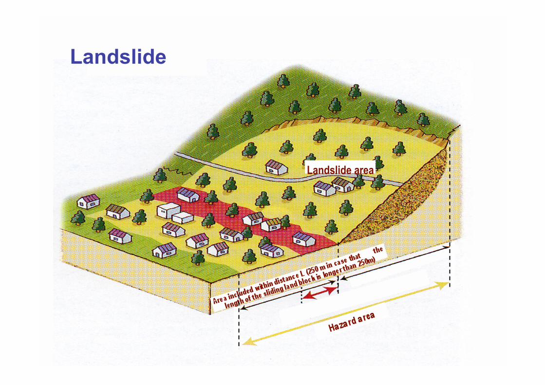
In effective stress condition (Terzaghi, 1925):

= shear strength (kN/m2)

c’ = effective cohesion (kN/m2)

’ = effective internal friction angle ( 0)

’ = effective normal stress on the failure plane (kN/m2)

u = pore water pressure (kN/m2)

Saturated soil

Mohr’s Circle and failure envelope

’

Failure

envelope

c f

3’ 1’ f’

2

1’

1’

3’ 3’ f’

f

1’ = effective major principle stress

3’ = effective minor principle stress

= theoretical angle between the failure plane and

major principal plane

Relationship between effective principle

stress at failure and shear strength

parameter c - :

Laboratory Test for Determination of

Shear Strength Parameter

1. Direct shear test

2. Triaxial test UU, CU CD

3. Unconfined compression test

4. Vane shear test

Direct Shear Test

N

T

Shear box

Porous stone

Sample

Loading

plate

h

L

Method of test :

Stress-controlled Test

Peak shear strength

Strain-controlled Test

Peak shear strength and Residual shear strength

Direct test is appropriate to be used for sandy soil.

Shearing the sample up to failure or the maximum strain

reaches max = 20%

Direst shear tests are repeated on similar specimens at

various normal stresses (min. 3 times).

1

2

3

c

1 2 3

Pure sand c = 0 ; maka

Dry condition :

Stress-strain characteristics of sand:

L

= constant

dense

loose

L H

+

-

Exp

an

sio

n

Co

mp

ressio

n

Dense sand

Loose sand

Peak shear strength

Residual shear strength

Shear displacement

Factors affected shear strength of sand:

- Particle size

- Water inter the particle

- Roughness of the surface of particle

- Grain size distribution

- Shape of particle

- Pore number (e) or relative density (Dr)

- Main principal stress

- Stress history

Example

Direct shear test on a clean compacted sand. Shear box with

dimension of 250 x 250 mm2. The results as follow:

Calculate shear strength parameter of the sand in dense condition

and loose condition

m dense sand peak stress

t loose sand residual stress

Normal force (kN) 5,00 10,00 11,25

Peak shear force (kN) 4,90 9,80 11,00

Residual shear force (kN) 3,04 6,23 6,86

Normal stress (kN/m2) 80 160 180

Peak shear stress (kN/m2) 78,4 156,8 176

Residual shear stress (kN/m2) 48,6 99,7 109,8

(kN/m2)

(kN/m2)

Peak stress

Residual

stress

From the above figure

m dense sand = 450

t loose sand = 320

Triaxsial Test

• The most reliable method to determine the shear strength

parameter of soil

• Commonly use for site investigation for civil construction and for research

h

h h

v

v

Applied stresses:

1 = major principal stress

3 = minor principal stress

2 = 3 = confining stress

= 1 - 3 = deviator stress

z

y

x 3

1

1

2

Correction of the sample area at a

certain strain (A)

Diagram of Triaxsial Test Equipment

Axial Load and Confining Pressure

3 3

3

3

3 3

3 + = 1

3 + = 1

L

Loading on vertical direction:

1. Apply the dead load gradually until failure. Axial deformation

is measured by dial gage.

2. Apply the axial deformation with a constant increment (strain-

controlled). Axial load is measured by proving ring.

Types of Standard Triaxial Test

Test condition 3 (confining

pressure)

Deviator stress,

Output

U.U.

(Unconsolidated-

Undrained)

Drainage

connection close

Drainage

connection

close

Total stress

C.U.

(Consolidated-

Undrained)

3 consolidation

Drainage

connection open

Drainage

connection

close

u

Total stress

Effective

stress

C.D.

(Consolidated-

Drained)

3 consolidation

Drainage

connection open

Drainage

connection

open

Effective

stress

The Results of Triaxsial test

(%)

31

32

33

c

3 1 1

f1

1 3 3

3 3

3 + = 1

3 + = 1

C.D. Test

3 3

3

3

uc=0 3 3

ud=0

3 + = 1

3 + = 1

B = pore pressure parameter by

Skempton (1954)

B = 1 for saturated soft soil

Confining

pressure Deviator

stress

t Vc

+

-

= constant

Dense sand / NC

Loose sand / OC

Vd

+

-

f

f

Dense sand / NC

Loose sand / OC

Because of the pore water pressure (u) during the

implementation of deviator stress is totally dissipated

Total stress = Effective stress

The same test is conducted at the same soil sample with

different 3 (confining pressure).

After getting 1 and 3 Mohr’s circle + failure envelope can be drawn

Failure envelope of Triaxsial CD

For sand dan clay NC

Failure envelope

3= 3’

2

1

1

3 3

f

f

2

1= 1’

A

B

f

f

Failure envelope of Triaxial CD

for clay OC

OC

BC

3= 3’

1

1

3 3

f

f

1= 1’

A

B

c

C

AB

NC

c= c’

C.U. Test

3 3

3

3

uc=0 3 3

ud 0

3 + = 1

3 + = 1

A = pore water pressure parameter

by Skempton (1954)

Confining

pressure Deviator

stress

t Vc

+

-

Dense sand / NC

Loose sand / OC

ud

+

-

f

f

Dense sand / NC

Loose sand / OC

Pore water pressure during the application of deviator stress = ud

Total stress Effective stress

Pore water pressure at failure can be measured = udf

Major principal stress at failure (total) :

Minor principal stress at failure (total) :

Pore water pressure at failure :

Major principal stress at failure (effective) :

Minor principal stress at failure (effective) :

In order to determine the shear strength parameter triaxial test

on soil samples should be done with different confining pressure 3

(%)

31

32

33

c

3 1 1

f1

1 3 3

3 3

3 + = 1

3 + = 1

Failure envelope of Triaxsial CU

For sand dan clay NC

Failure envelope

of effective stress

3

1

1

3 3

f

f

1

A

B

udf

C

D

cu

1’ 3’

udf

Failure envelope

of total stress

OC

2

3

1

1

3 3

f

f

1

A

B

c

C

1

NC

c

Failure envelope of Triaxial CU

for clay OC

A parameter for clay:

• Lempung NC : 0,5 – 1

• Lempung OC : -0,5 – 0

A value depends on OCR

c’ = c = maximum confining pressure when the soil sample consolidates

A = pore water pressure parameter by Skempton

(1954) at failure:

U.U. Test

3 3

3

3

uc 0 3 3 ud 0

3 + = 1

3 + = 1

Confining

pressure Deviator

stress

Total pore water pressure =

and

Hence

Triaxial UU test on saturated clay :

f will be the same for different confining pressure 3

Failure envelope

1

1

3 3

f

f

cu

3 1 1 3 3 1

The application of Triaxial UU, CU and CD:

UU :

• Foundation on soft soils

• Embankment on soft soils

• Dam on soft soils

The loading apply so fast, hence the consolidation and drainage

did not occur yet at the soil layers end of construction

CU :

• Slope stability, where the soil has been consolidated and stable

• Rapid draw-down at of reservoir

• Embankment construction (several phase / stage)

CD :

• Embankment long time construction

• Earth dam affected by steady

• Clay excavation

• Practically, it is difficult to implement this test for clay,

because the time to get u = 0 will be too long,

p = need to be small it takes a long time and very easy to seep out.

Example 1

Triaxial CD has been done for normally consolidated clay.

The result of test as follow:

3 = 276 kN/m2

f= 276 kN/m2

Calculate :

a. Internal friction angle,

b. The angle between failure surface and major principal plane,

c. Normal stress ’ and shear stress f at failure surface

For Normally Consolidated Clay, the failure envelope equation

Principal stress:

Failure envelope

3’=276 kN/m2

2

’1

’1

’3 ’3

f

f

B

1’=552 kN/m2 A O

Failure

envelope

3’=276 kN/m2

2

B

1’=552 kN/m2 A O

At failure

plane

Example 2

Consolidated-Drained Triaxial test for example no. 1 :

a. Calculate effective normal stress ( ’) acting on the plane with

maximum shear stress ( ).

Maximum shear stress occurs at the plane with = 450

b. Why does the failure occur at the plane of = 54,730, not at the

plane having maximum shear stress?

Shear stress that causes the failure at = 450:

Shear stress acting on that plane :

Example 3

The result of triaxial test (UU) as follow:

Calculate the shear strength parameter by using Mohr’s circle.

No of test Confining pressure

(kg/cm2)

Deviator stress (kg/

cm2)

1 1 0,57

2 1,4 0,71

3 1,8 0,76

4 2,2 0,84

(kg/cm2)

Failure envelope

c

33 13 14 34 32 12

1 2 3

(kg/cm2)

1

No test 3 (kg/cm2) (kg/cm2) 1= 3+

(kg/cm2)

( 1+ 3)/2

(kg/cm2)

1 1 0,57 1,57 1,285

2 1,4 0,71 2,11 1,753

3 1,8 0,76 2,56 2,182

4 2,2 0,84 3,04 2,620

From the figure :

Example 4

Triaxial test (CU) for normally consolidated clay, with the result:

3 = 260 kN/m2

Deviator stress : f= 200 kN/m2

Pore water pressure : udf = 120 kN/m2

Calculate :

a. Internal friction angle at Consolidated-Undrained (CU)

condition

b. Internal friction angle at Consolidated-Drained (CD) condition

Unconfined Compression

Test

(Uji Tekan Bebas)

Unconfined

Compression Test

as a special type of

Triaxial UU for

saturated clay

ASTM D2166

AASHTO T208

1

1

3=0 cu

3=0 1=qu

qu = unconfined compression

strength

Consistency qu (kN/m2)

Very soft 0 – 25

Soft 25 – 50

Medium 50 – 100

Stiff 100 – 200

Very stiff 200 – 400

Hard >400

Theoretical failure envelope

of total stress

cu

3 1 1 3 0 1=qu

The real failure envelope

of total stress

1 2

3

Result of Unconfined Compression Test (Mohr’s circle-1)

vs. Triaxial UU (Mohr’s circle- 2 and 3) for saturated clay

Vane shear Test

To determine shear strength at undrained condition cu ( = 0)

for saturated clay.

Method:

• Vane shear equipment is driven to

the borehole with minimum depth of

3 x borehole diameter

• Rotate with the velocity of 6o – 12o per minute.

• Every 15-30 seconds, record T value

h

d

Ms

Me

Me cu

cu

cu

Shear strength mobility at 2

cylindrical edge surface

Bjerrum (1974) : cu form vane shear test is too high, because of

the shear zone expanded.

Vane shear result in the field need to be corrected:

= correction factor = 1,7 – 0,54 log (PI) See HCH MT1 :

5.2.4 page 305

PI = Plasticity index = LL - PL

cu vs o’

Clay NC :

(Skempton, 1957)

o’ = effective overburden pressure

IP = plasticity Index (%)

Clay OC :

(Ladd et al., 1977)

The other method to decide undrained shear strength:

Torvane

Pocket penetrometer

Sensitivity and Thixotropy of clay

1

Axial strain

undisturbed

remolded

qu

qu

Sensitivity Classification

4 – 8 Sensitive clay

8 – 16 Extra sensitive

clay

> 16 Quick clay

From unconfined

compression test

Example :

Result of Unconfined Compression Test:

Calculate the shear strength parameters.

Solution: Draw the relation between Strain ( ) vs Stress ( )

Strain (%) Stress (kg/cm2)

1 0,268

5 0,450

7 0,46

8 0,47

9 0,46

12 0,45

(kg/cm2)

(%)

qu

0 5 10 15 20

0,5

0,4

0,3

0,2

0,1

cu

3=0 1=qu

Ko (Lateral Earth Pressure Coefficient)

(Lateral earth pressure coefficient)

Depend on and stress history

Ko for sand

Ko value for sand OC > sand NC

Sand OC

h = 0,4 – 0,5

h = 0,6 (dense sand)

(Jaky, 1944)

(Schmidt,1967 & Alphan,1967)

Ko for clay

See HCH MT1 Figure 5.42 Page 366

(Massarch, 1979)

Slope stability analysis

1. Transitional movement

2. Rotational movement (circular slip

surface)

3. Method of slice

4. Slope stability software for 2D analysis

5. 3D landslide movement simulation

Slope Stability Analysis

• Slope stability concept: limit plastic equilibrium

• Purpose to determine the safety factor (FS) of the potential slip

surface

• Assumption:

Sliding occurs at a certain slip surface 2 dimensional

problem

Sliding material massif

Isotropic shear strength

FS is analyzed based on average shear strength at the slip

surface

Difference between landslide and slope failure Landslides Slope Failures

Geology Occur in places with particular

geology or geological formation

Slightly related to geology

Soils Are mainly active on cohesive

soil such as slip surface

Frequently occur even in sandy

soils

Topography Occur on gentle slopes of 5° to

20°

Frequently occur on the slopes

steeper than 30°

Situation of

activities

Continuous, or repetitive

occurrences

Occur suddenly

Moving velocity Low at 0.001 to 10 mm/day High speed > 100 mm/day

Masses Have little disturbed masses Have greatly disturbed mass

Provoking causes Greatly affected by groundwater Affected by rainfall intensity

Scale Have a large scale between 1

and 100 ha

Have a small scale. Average

volume is about 440 m3

Symptom Have cracks, depressions,

upheavals, groundwater fluctuation, before occurrence

Have few symptoms and

suddenly slip down

Gradient 10° to 25° 35° to 60°

Slope failure

Steep slope area

Hei

gh

t o

f st

eep

slo

pe

(h)

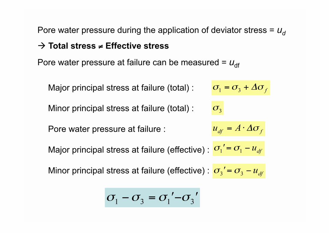
Landslide area

Landslide

Tsaoling Landslide

Induced by 1999 Chi-chi

Earthquake, Taiwan

Volume: 1.4 x 108 m3

Affected area: 698 ha

Total length: 4 km

Source area:

Length: 1.5 km

Width: 2 km

Depth: < 200 m

Destruction of 5 houses,

resulting in 29 deaths.

Causes of Landslide

• Rainfall or storm rainfall the rising of

groundwater level

• Construction works Earthwork, Cutting,

Filling, Tunnel construction,

• Reservoir induced landslide the rising and

drawdown of reservoir level

• Earthquake horizontal acceleration gx, gy

Shear Strength Parameters

Shear strength parameter:

Internal resistant force per unit area

Failure of shear at a slip surface due to applied force to the soil.

Shear resistant:

1. Cohesion (c): depend on the type of soil and its density,

independent from normal stress ( ) at the shear surface.

2. Friction inter material ( tan ): depend on the normal

stress ( ) at the shear surface and internal friction angle ( )

3. Combination of c and

MOHR-COULOMB Failure Criteria

Mohr (1900): Failure of a material due to the combination of critical

condition between normal stress ( ) and shear stress ( )

Coulomb (1776) f ( ) :

N

F

A

= shear strength (kN/m2)

c = cohesion (kN/m2)

= internal friction angle ( 0)

= normal stress at the failure

surface (kN/m2)

MOHR-COULOMB Failure Criteria

Mohr

Mohr-Coulomb

c

A

B

C

y

x

f

A Failure does not occur

B Failure occurs

C Failure never happen

In effective stress condition (Terzaghi, 1925):

c’ = effective cohesion (kN/m2)

’ = effective internal friction angle ( 0)

’ = effective normal stress (kN/m2)

u = pore water pressure (kN/m2)

= average shear stress

d = average shear stress at the critical slip surface due to the weight of

sliding material

Mohr-Coulomb

c- = shear strength parameter at the critical slip surface

SLOPE STABILITY

Safety factor for cohesion component

Safety factor for friction component

In general FS 1,2

FS = Fc = F

Analysis on a translational slip surface

A. Infinite slope

A.1. Without seepage

W

P

Na

Ta

Tr

Nr

E

E

A

B

P

Q

S

T H

b

Bedrock

W

P

Na

Ta

Tr

Nr

E

E

A

B

P

Q

S

T H

b

Bedrock

If F = 1 (critical), so H = Hc:

Granular soil (c = 0)

Cohesive soil ( = 0)

F = 1 (critical), ( = 0): Stability number

W

P

Na

Ta

Tr

Nr

E

E

A

B

P

Q

S

T H

b

Bedrock

A.1. With seepage

W

P

Na

Ta

Tr

Nr

A

B

P

Q

S

T H

b

Bedrock

Hcos

2

Due to water flow

shear strength:

Granular soil (c = 0)

Cohesive soil ( = 0)

Example 1

H

Bedrock

= 1,86 t/m3

c =1,8 t/m2

=20o

a) H = 8 m ; = 22o calculate FS & Hc

b) H = 8 m ; = 25o , Calculate FS and Hc

Example 2

H

Bedrock

sat = 2 t/m3

c =1,8 t/m2

=20o

If H = 8 m ; = 22o ; calculate FS

Analysis on a translational slip surface

B. Finite slope

B.1. Culman’s method

W

P

Na

Nr

Ta

Tr

H

A

B C

W

P

Na

Nr

Ta

Tr

H

A

B C

Shear resistant ( d) at AB:

Critical condition F=1

= d

Critical condition

F=1 cd = c ; d =

Example 1

H = ?

Previous

landfill

New landfill

timb = 1,96 t/m3

c =2,5 t/m2

=17o

= 48,5o

= 40o Calculate the maximum height of

new landfill, if the safety factor is

decided to be F=2

W

P

Na

Nr

Ta

Tr

H=5 m

A

B C

Example 2

= 19 kN/m3

c = 25 kN/m2

=12o

= 52o

= 30o

B. Finite slope

B.2. Analysis on a circular slip surface

O

(a) Toe circle

O

(b) Slope circle

bedrock

O

(c) Shallow slope circle

O

(d) Mid circle

L L

bedrock

Slope stability analysis on cohesive soil

OWithout

groundwater

y

W R

A

B C

C

= 0

W = weight of sliding material (kN)

LAC = length of circular plane (m)

c = cohesion (kN/m2)

R = radius of slip surface circle (m)

y = distance between W to point O (m)

OWith the

existence of

groundwater

W

R

A

B C

C

= 0

W’ = effective soil weigth (kN)

LAC = length of circular slip surface (m)

c = cohesion (kN/m2)

R = radius of slip surface circle (m)

y = distance between W’ to point O (m)

W’

U

Slope stability analysis on cohesive soil

Slope stability analysis on cohesive

soil, using Taylor Diagram (1948)

W1 = area (EFCB) x x 1

W2 = area (EFDA) x x 1

O

y1

W1

R

A

B C

Cd

= 0

D F

E

W2

y2

Nd

= angle from the figure in radian

Equilibrium condition

O

y1

W1

R

A

B C

Cd

= 0

D F

E

W2

y2

Nd

R trial and error minimum FS

O

y1

W1

R

A

B C

Cd

= 0

D F

E

W2

y2

Nd

Critical condition (F=1); H = Hc ; cd = cu

Taylor Method (1948)

Stability number:

Nd value is decided by using STABILITY DIAGRAM : =0 Taylor (1948)

Depth factor, D

Slope angle,

Example:

Excavation of 10 m depth in saturated cohesive soil. Unit volume of

saturated clay is 18,5 kN/m3 and cohesion is 40 kN/m2. Bedrock located

at 12 m below the surface. If the internal friction angle of the soil is =

0, calculate the inclination of the slope if the safety factor is decided to

be F=1,5.

Depth factor : D = 12/10 = 1,2

Depth factor, D

Slope stability analysis for the soil > 0,

using Taylor Diagram (1948)

If the soil has the friction component ( ) normal stress distribution (N)

affect the distribution of shear stress

Normal stress resultant and friction component have the inclination of

based on normal line direction

O

R

A

B C

D F

E

Critical condition F=1:

Slope inclination,

Contoh:

An earthfill H =12,2 m, = 30o. Bedrock at infinite depth. C = 38,3 kN/m2,

= 10o and total unit weigth = 15,7 kN/m3. Calculate safety factor of

cohesion (Fc), to internal friction (F ) and overall safety factor (F).

a. Assuming all works = 10o ; = 30o

From figure cd/ H = 0,075 cd = 14,4 kN/m2

Fc = c/cd = 38,3 / 14,4 = 2,67

b. Assuming all c works c = 38,3 kN/m2 ; = 30o ; cd/ H = 0,2

From figure < 0 F =

(Resistant moment due to cohesion > driving moment)

c. F to shear strength by trial and error

All works F = 1 Fc = 2,67

Fc = c/cd = 2 cd = 38,3/2 = 19,2 kN/m2 cd/ H = 0,1 From figure d = 7o F = tan 10o / tan7o = 1,44

Fc = c/cd = 1,8 cd = 38,3/1,8 = 21,3 kN/m2 cd/ H = 0,11 from figure d = 5o F = tan 10o / tan5o = 2,02

Slope stability analysis

Method of slice

Stability Analysis of Landslide Slope

The design of a slope should ideally be based on an

allowable deformation

The difficulty with deformation analysis stress-strain

relationship, peak and residual strengths, anisotropic, pore

pressure distribution, the non-homogeneity, and the effect due to initial stress.

Finite element method reflecting all of the factors.

As an alternative, a limit equilibrium analysis stability of a

slope, in terms of a safety factor F.

Limit equilibrium method analysis of natural & artificial

slopes (cut and fill)

No Method Equilibrium equation

Force Moment

Horizontal Vertical

1 Fellenius (1927) – –

2 Bishop’ Simplified (1955) –

3 Janbu’s Simplified (1954) –

4 Corps of Engineering (1982) –

5 Lowe and Karfiath (1960) –

6 Spencer (1967)

7 Sarma (1973)

8 Morgenstern and Price (1975)

Slope stability analysis based on the limit equilibrium

and slice method

Remarks :

” ” : The equilibrium of horizontal forces, vertical forces or moments are taken into account for analysis.

Circular slip surface

Bishop Method

Fellenius Method

These methods are currently being widely used in

the field of landslide analysis.

O x

R

n n+1

W

Xn En

Xn+1

En+1

h

b

P C

B

ls

A

D

l

W

Xn-Xn+1

En-En+1

S

P

P’

ul

tan =1/F.tan ’

Bishop method

The Bishop method is a method for analyzing the equilibrium of a sliding

block, which slumps in a single movement about a given point.

The equilibrium equation for moments about the center of rotational

movement is expressed as :

The Mohr-Coulomb failure criterion is :

Bishop method

In solving stability problems determine statically indeterminate elements,

obtaining equilibrium among the slice in horizontal and vertical directions.

In the simplified Bishop method, horizontal forces are ignored, and only the

vertical forces in each slice are taken into account:

Since both sides of expression contain F, the safety factor has to

be obtained by a series of calculations.

O x

R

n n+1

W

Xn En

Xn+1

En+1

h

b

P C

B

ls

A

D

l

Fellenius

method Internal forces applied to the wall

of each slice are ignored:

The moments of the entire

sliding block are in equilibrium:

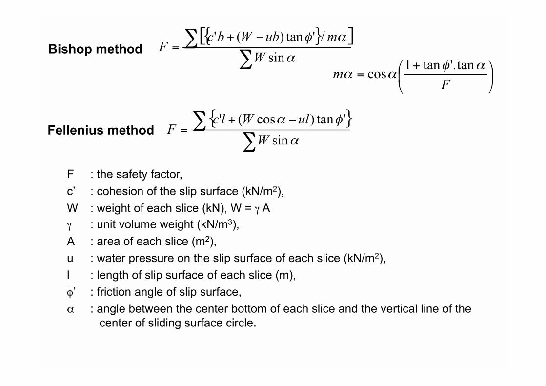
Bishop method

Fellenius method

F : the safety factor,

c’ : cohesion of the slip surface (kN/m2),

W : weight of each slice (kN), W = A

: unit volume weight (kN/m3),

A : area of each slice (m2),

u : water pressure on the slip surface of each slice (kN/m2),

l : length of slip surface of each slice (m),

’ : friction angle of slip surface,

: angle between the center bottom of each slice and the vertical line of the

center of sliding surface circle.

Non-circular slip surface

Janbu Method

Morgenstern and Price Method

Janbu method : an analytical method for analyzing the stability of a

landslide block sliding surface has a complex shape

Janbu Method

where fo is a modifying coefficient representing the influence of the

shearing force acting on the walls of each slice.

The coefficient can be decided from analysis of soil and other

conditions, covering more than 40 different cross sections.

1 2

3

i

n

x

y

Ei

Xi

Ni

Ti

Xi+ Xi

Ei+ Ei

kHWi

(1+kV)Wi i

Simplified Janbu’s method

where

Janbu’s correction factor :

Calculate the safety factor by using the ordinary method of slice