Energy Harvesting from Rainwater and Maximum Power Point ... · Crossflow turbine, and Pelton wheel...

Carolyn Detora, Kayleah Griffen,

Nicole Luiz, and Basak Soylu

Worcester Polytechnic Institute

Energy Harvesting from Rainwater and Maximum Power Point Tracking Solar Charging

1

Abstract

The primary purpose of this project was to provide electricity that was sufficient for

powering lights and charging cell phones in rainy locations with limited electricity access. A

household rainwater energy harvesting system was researched, designed, prototyped, and tested to

determine the feasibility of rainwater as a source of renewable energy. The system prototyped

consisted of a gutter assembly that collected and funneled water from the roof to a downspout. The

downspout shielded the stream of water from wind and directed it to a turbine at the ground level.

The turbine was connected through a gear train to a DC motor serving as the generator. The device

is optimal during high rainfall intensities that produce larger flow rates. An Overshot water wheel,

Crossflow turbine, and Pelton wheel turbine were evaluated under 8, 6, 4, and 2 gallons per minute

flow rates using a tachometer and a torque meter. These flows were based on Liberian rainfall

intensities scaled to a representative house that was 5 by 3 meters in roof area. The most suitable

turbine was a 20 centimeter diameter Pelton wheel with 23 equally spaced blades. A micro gear

motor rated at a maximum speed of 460 RPM and a stall torque of 20 ounce-inch was selected to

serve as the generator. The system produced a power of 0.74 Watts and a 14.8% efficiency at 8

GPM. When scaled for the rainfall in the month of June, the current system could charge about 1.8

cell phones. This project proved the concept and design of a rainwater energy harvesting system.

The system could be combined with a filtration system and holding tank to collect drinkable water

so that the system serves a dual purpose for people with limited access to electricity and water. The

secondary purpose of this project was to examine solar charging and develop a maximum power

point tracking solar energy charger that complemented the work of another MQP: Mapping Urban

Pollution. The solar energy charger design involved MATLAB Simulation and the construction of

the solar energy charger with a 2W solar panel, a DC/DC boost converter, a battery and a

microcontroller to do the maximum power point tracking, this portion is all described in Chapter 6.

2

Table of Contents Abstract ................................................................................................................................................................................ 1

Table of Figures .................................................................................................................................................................. 4

1.0 Introduction ........................................................................................................................................................... 6

2.0 Background ............................................................................................................................................................ 8

2.1 Types of Hydropower ...................................................................................................................................... 8

Storage Hydropower ................................................................................................................................................. 8

Pumped-Storage Hydropower ................................................................................................................................. 9

Offshore Hydropower .............................................................................................................................................. 9

Run-of-River Hydropower ....................................................................................................................................... 9

2.2 Types of Turbines........................................................................................................................................... 10

Impulse Turbines ..................................................................................................................................................... 10

Reaction Turbines .................................................................................................................................................... 12

Waterwheels .............................................................................................................................................................. 13

2.3 Pico-Hydro Power Generation ............................................................................................................................ 14

2.4 Electrical Components .......................................................................................................................................... 14

2.5 Energy Harvesting from Rainwater for Household Systems .......................................................................... 16

3 Design and Construction ........................................................................................................................................ 18

3.1 System Components, Initial Design, and Project Scope ................................................................................. 18

Project Scope ............................................................................................................................................................ 19

3.2 Initial Power Calculation....................................................................................................................................... 20

3.3 Prototype for Testing Structure ........................................................................................................................... 29

3.4 Gutter and Downspout Sub-System ................................................................................................................... 32

Gutter Sizing and Slope .......................................................................................................................................... 32

Gutter-to-Downspout Connection Types ........................................................................................................... 43

Gutter-to-Downspout Connection Tests ............................................................................................................ 45

Downspout Consideration ..................................................................................................................................... 51

3.5 Turbine Selection ................................................................................................................................................... 52

Description and 3D Printing of Turbines for Preliminary Testing ................................................................. 53

SolidWorks Simulations .......................................................................................................................................... 56

Preliminary Stall Torque and RPM Testing ......................................................................................................... 62

Design and Optimization of Pelton and Crossflow ........................................................................................... 63

Final Turbine Selection ........................................................................................................................................... 66

3.6 Electrical Component Selection .......................................................................................................................... 72

3.7 Design Tree Summary ........................................................................................................................................... 77

3

4.0 Testing and Results .................................................................................................................................................... 78

4.1 RPM and Torque Testing ..................................................................................................................................... 78

RPM and Torque Testing Results ......................................................................................................................... 79

Theoretical Validation of RPM and Torque Testing ......................................................................................... 80

4.2 Full System Testing................................................................................................................................................ 83

Full System Testing ................................................................................................................................................. 83

Theoretical Determination of the Angular Velocity in the Full System Results ........................................... 85

4.3 Loss Considerations and Efficiency.................................................................................................................... 86

5.0 Conclusions and Recommendations ....................................................................................................................... 88

5.1 Expenses.................................................................................................................................................................. 88

5.2 Recommendations for Future Work................................................................................................................... 89

6.0 Maximum Power Point Tracking Solar Charger ................................................................................................... 91

6.1 Solar Panel and Battery Selection ........................................................................................................................ 92

6.2 Maximum Power Point Tracking Using Boost DC/ DC Converter ............................................................ 94

6.3 Sensing Solar Panel Voltage, Current, Power .................................................................................................... 99

6.4 Sensing Battery Voltage ...................................................................................................................................... 100

6.5 Overall Schematic and Control Algorithm of Maximum Power Point System ......................................... 101

6.6 Practical Model of the Solar Panel .................................................................................................................... 102

6.7 Simulation of the Solar Charging System ......................................................................................................... 105

6.8 Experimental Results from the Solar Charging System ................................................................................. 106

6.9 Recommendations for Future Work................................................................................................................. 109

References Chapters 1-5 ................................................................................................................................................ 110

References Chapter 6 ..................................................................................................................................................... 112

Appendix A: Sizing of Rectangular and Half Round Gutters for English and Metric Units ............................. 114

Appendix B: Overshot Water Wheel Assembly Drawings ..................................................................................... 116

Appendix C: Pelton Wheel Assembly Drawings ....................................................................................................... 117

Appendix D: Crossflow Turbine Assembly Drawings ............................................................................................. 118

Appendix E: SolidWorks Static Simulations – Overshot Water Wheel ................................................................. 119

Appendix F: SolidWorks Static Simulations – Pelton Wheel .................................................................................. 120

Appendix G: SolidWorks Static Simulations – Crossflow Turbine ........................................................................ 121

Appendix H: Arduino IDE MPPT Code.................................................................................................................... 122

Appendix I: MATLAB Practical Model Parameter Extraction Code .................................................................... 125

Appendix J: MATLAB Practical Model Characteristic Curve Plotting Code ....................................................... 126

Appendix K: MATLAB Simulink Practical Model Solar Panel with DC to DC Converter............................... 129

Appendix L: Maximum Power Point Tracking Code written in MATLAB.......................................................... 130

4

Table of Figures Figure 1: Example Pelton Wheel ................................................................................................................. 11 Figure 2: Example Crossflow Turbine .......................................................................................................... 11 Figure 3: Example Propeller Turbine........................................................................................................... 12 Figure 4: Example Archimedes Screw ......................................................................................................... 12 Figure 5: Example Overshot Water Wheel ................................................................................................. 13 Figure 6: Example Backshot Water Wheel .................................................................................................. 13 Figure 7: DC Motor Rotational Speed vs Torque ........................................................................................ 15 Figure 8: Assembly of Turbine .................................................................................................................... 17 Figure 9: Initial Design ................................................................................................................................. 19 Figure 10: Home in Liberia with Corrugated Roof ...................................................................................... 20 Figure 11: Circular Segment Filled by Water .............................................................................................. 24 Figure 12: Theoretical Power Output of the Turbine vs Rainfall Intensity ................................................. 27 Figure 13: Design of Test Structure ............................................................................................................. 29 Figure 14: White Vinyl Hidden Hangers ...................................................................................................... 30 Figure 15: Assembled Gutter ...................................................................................................................... 31 Figure 16: Exploded View of Turbine Stand ................................................................................................ 32 Figure 17: Depiction of Single Corrugation ................................................................................................. 33 Figure 18: Velocity Components ................................................................................................................. 36 Figure 19: Elbow Connectors and Short Lengths of Downspout ................................................................ 43 Figure 20: Straight Downspout ................................................................................................................... 44 Figure 21: Open End Gutter ........................................................................................................................ 44 Figure 22: Vertical Downspout ................................................................................................................... 45 Figure 23: Bent Downspout ........................................................................................................................ 46 Figure 24: Funnels Placed on Top of Downspout ....................................................................................... 46 Figure 25: Stream Size for (a) Vertical Downspout, (b) Bent Downspout, (c) 1.4 centimeter Funnel, (d) 1.1 cm Funnel .................................................................................................................................................... 47 Figure 26: CAD Model of Overshot Water Wheel ....................................................................................... 53 Figure 27: 3D Printed Overshot Water Wheel (a) Front View (b) Side View .............................................. 53 Figure 28: CAD Model of the Pelton Wheel ................................................................................................ 54 Figure 29: 3D Printed Pelton Wheel (a) Front View (b) Side View .............................................................. 54 Figure 30: CAD Model of Crossflow Turbine ............................................................................................... 55 Figure 31: CAD Model for 3D Printing of Crossflow Turbine (a) Top of Turbine (b) Blades and Bottom of Turbine ........................................................................................................................................................ 55 Figure 32: 3D Printed Crossflow Turbine (a) Top View (b) Side View ......................................................... 56 Figure 33: Steps for SolidWorks Simulation ................................................................................................ 57 Figure 34: Stress-Strain Curve of ABS ......................................................................................................... 58 Figure 35: Overshot Water Wheel Pressure Points on SolidWorks Simulation .......................................... 58 Figure 36: Overshot Water Wheel Static Stress SolidWorks Simulation Results ........................................ 59 Figure 37: Pelton Wheel Pressure Points on SolidWorks Simulation ......................................................... 59 Figure 38: Pelton Wheel Static Stress SolidWorks Simulation .................................................................... 60 Figure 39: Crossflow Turbine SolidWorks Simulation Pressure Points ....................................................... 61

5

Figure 40: Crossflow Turbine Static Stress SolidWorks Simulation ............................................................ 61 Figure 41: Optimized Pelton Wheel 20 centimeters (a) Top View (b) Side View ....................................... 65 Figure 42: Optimized Crossflow Turbine 20 centimeter (a) Top View (b) Side View .................................. 66 Figure 43: Torque Angular Velocity and Angular Relationships ................................................................. 69 Figure 44: Maximum Power Calculations Pelton vs Crossflow ................................................................... 70 Figure 45: Series of Two Spur Gears ........................................................................................................... 72 Figure 46: System Motor............................................................................................................................. 75 Figure 47: Motor in the Casing.................................................................................................................... 75 Figure 48: Generator Encasement .............................................................................................................. 76 Figure 49: Design Tree Summary ................................................................................................................ 77 Figure 50: Theoretical and Maximum Calculated Power Outputs of the Turbines vs. Rainfall Intensity at a Height of 2 Meters ...................................................................................................................................... 80 Figure 51: Maximum Power Calculated and Actual Power Outputs of the Turbines vs. Rainfall Intensity 84 Figure 52: Efficiency Flow Chart .................................................................................................................. 86 Figure 53: Voltage vs Power Curve for 2W Solar Panel .............................................................................. 95 Figure 54: Basic Layout of DC/DC Boost Converter .................................................................................... 96 Figure 55: Varying the Inductor and Capacitor Size and its Effects on the Power v Duty Cycle Graph ...... 98 Figure 56: Solar Charging Boost Converter Topology ................................................................................. 99 Figure 57: Voltage follower and Voltage Divider Circuit ........................................................................... 100 Figure 58: Full Solar Charging System Schematic ..................................................................................... 101 Figure 59: Solar Panel Practical Model ..................................................................................................... 103 Figure 60: Characteristic IV and PV Curves for Solar Panel ...................................................................... 104 Figure 61: Effect of Duty Cycle Step Size on Maximum Power Point Tracking ......................................... 105 Figure 62: Full System Constructed .......................................................................................................... 106 Figure 63: The IV and PV Characteristic Curves for the Solar Panel ......................................................... 107 Figure 64: Maximum Power Point Tracking Test Case .............................................................................. 108 Figure 65: Voltage Varying as a Result of Irradiance Level Changing ....................................................... 108

6

1.0 Introduction

The global energy consumption was 575 quads in 2015, and is expected to increase by 28%

by the year 2040 (“International Energy Outlook”, 2017). Renewable energy is becoming the fastest

growing energy type as countries switch from fossils fuels to various renewable sources. The

benefits of obtaining energy from sources such as the sun, wind, and water are trifold. Renewable

energy is helping tackle climate change, energy security, and energy access.

A global transition to renewable energy not only would combat climate change, but also has

the potential to close the gap between those with and without electricity. There is a connection

between access to electricity and the ability for economic and human development to occur, termed

energy poverty (González-Eguino, 2015). In today's world, over 1.4 billion people face energy

poverty. The challenge of energy poverty is concentrated in rural areas, where 85% of the

population lacks electricity access (Stram, 2016). Rural renewable electrification programs are an

opportunity to help combat energy poverty.

Our Major Qualifying Project will work to target rural electrification and clean water access

in areas with high levels of rainfall through a rainwater collection and pico-hydropower harvesting

device. Accessing water is an energy intensive process and recognizing the intersection between

energy and water and using rainwater harvesting to approach the problem is a research area being

pursued (Vieira, Beal, Ghisi & Stewart, 2014). The goal of our project is to create a pico-hydropower

energy collection device that can be implemented into a rainwater harvesting system in order to

provide electricity when solar energy is not available. Our project will target the needs of rural

Liberia, where 70% of the population lives in multidimensional poverty, and of the rural population

only 1.2% of people have access to electricity and 56% have access to improved drinking water

(United Nations Development Programme, 2016; Liberia Institute of Statistics and Geo-

Information Services, 2013). More than 40% of the people living in rural Liberia have access to a cell

7

phone or a radio and almost all of the rural population has some method for accessing lighting;

(Liberia Institute of Statistics and Geo-Information Services, 2013). The development of technology

tailored to the social and cultural needs of specific rural areas is critical to their success (Urmee &

Md, 2016). In our project we will not delve deep into the social side of the pico-hydropower energy

and rainwater harvesting system, however we have assessed the rural electricity uses and strategies

for accessing water. Our project will work to target the scarcity in rural electricity and water through

the development of a rainwater energy harvesting system.

8

2.0 Background

In this section we will discuss the various types of hydropower, the types of turbines

commonly used in hydropower systems, and electrical generators. We will also investigate pico-

hydro power generation from rainfall to gain a better understanding of the requirements for our

system in rural Liberia.

2.1 Types of Hydropower

Historically, hydropower systems converted the energy in water to produce mechanical

work. Such systems performed a variety of industrial activities, such as milling grains. Present day

hydropower systems convert stored energy in water into electricity, instead of mechanical work. The

power output for hydropower installations range from a few kilowatts to gigawatts. At 1,064

gigawatts of installed capacity, hydropower is the leading source of renewable energy and accounts

for 71% of all renewable electricity (World Energy Council, 2016). Overall, 16.4% of the world’s

total electricity is generated from hydropower systems (World Energy Council, 2016). There are four

main types of hydropower: storage hydropower, pumped-storage hydropower, offshore

hydropower, and run-of-river hydropower (World Energy Council, 2016).

Storage Hydropower

Storage hydropower systems capitalize on the potential energy of water contained by a dam

structure. To produce electricity, water is released from the dam and flows through a turbine. The

rotating turbine activates a generator to produce electricity. Storage hydropower provides base load,

a continuous supply of electricity, and peak load, the ability to be turned off and restarted based on

demand (World Energy Council, 2016).

9

Pumped-Storage Hydropower

Pumped-storage hydropower is similar to storage hydropower, except that these systems

cycle the water between upper and lower reservoirs to provide peak-load supply. When electricity is

needed, water from an upper reservoir is released and spins a turbine. The potential energy of the

elevated water produces the electricity. When electricity demand is low, pumps use extra energy in

the system to drive the water back to the top reservoir to prepare for the next cycle (World Energy

Council, 2016).

Offshore Hydropower

Offshore hydropower systems use waves and tidal currents in the ocean to produce

electricity. Among the different types of hydropower, offshore is the least established, but still

growing. This category includes technology such as underwater turbines (tidal), buoys (wave), and

oscillating water columns (wave) (Tester, Drake, Driscoll, Golay & Peters, 2016, p. 700).

Run-of-River Hydropower Run-of-river hydropower produces electricity as the flowing water, typically from a river or

channel, spinning a turbine. The kinetic energy of the flowing water is used to produce electricity,

unlike in storage hydropower systems where the potential energy is the driving factor (World Energy

Council, 2016). Run-of-river systems produce a continuous supply of electricity. However, there are

other much smaller forms of run-of river hydropower such as Ultra Low Head Hydroelectric

technology for heads less than 3m and flows greater than 0.5 meter per second with no head that are

currently being explored (Zhou & Deng, 2017). This indicates that although hydropower technology

has been around for a long period of time, new and exciting innovations are still being explored.

10

2.2 Types of Turbines

In hydropower systems, two main types of turbines exist: reaction and impulse. Impulse

turbines use the velocity of the water to rotate the shaft, and are typically suitable for high heads and

low flow applications (“Comparison between Impulse and Reaction Turbine,” 2016). Impulse

turbines that are typically considered for small hydropower systems are the Pelton wheel, Turgo, and

Crossflow turbines. Reaction turbines generate power from the combined pressure and moving

water. They are typically submerged so that water flows over the blades, rather than striking them.

This type of turbine is typically suitable for low head and high flow applications. A major difference

between the two types of turbines is that reaction turbines must be enclosed in a watertight casing,

while impulse turbines do not (“Comparison between Impulse and Reaction Turbine,” 2016). The

types of reaction turbines that are typically used for small hydropower systems are propellers, such

as: Kaplan turbines, and Archimedes screws. In addition, we are considering water wheels as an

alternative to a traditional turbine. Water wheels differentiate from turbines because they generate

energy from the weight of the water rather than from the water’s velocity or impulse (“Waterwheel

Design and the Different Types of Waterwheel,” 2013). The type of water wheels that are the most

applicable are the Overshot and the Backshot water wheels, because the source of water comes from

above, as opposed to below.

Impulse Turbines

Pelton wheel- Pelton wheels consist of multiple bucket-shaped blades, known as impulse

blades, and often have jets directed tangential to the turbine, Figure 1. Each individual blade has two

“buckets” that are connected in the middle. This type of turbine is most applicable with high heads

(greater than 25 meters) and low flows (0.01-0.5 cubic meters per second), but has been modified for

application in micro-hydro systems (Okot, 2013).

11

Figure 1: Example Pelton Wheel

(Picture Credit: Jahobr Water Wheel, 2018)

Turgo turbine- The Turgo turbine is a modification of the Pelton wheel, except it uses only

half of the blade, or just one “bucket.” Similar to the Pelton, the jets are aimed tangential to the

turbine. This turbine functions in similar heads and flows to the Pelton wheel, but can have more

efficient operations in lower head ranges (Okot, 2013).

Crossflow- The Crossflow turbine is designed with tangential rectangular-shaped blades that

allow the water to flow through the turbine twice, flowing through the inside of the runner, Figure 2.

This turbine is applicable in low to medium heads (2- 40 meters) and low to medium flows (0.1- 5

cubic meters per second) (Okot, 2013). The Crossflow turbine maintains efficiency under varying

load and flow.

Figure 2: Example Crossflow Turbine


12

Reaction Turbines

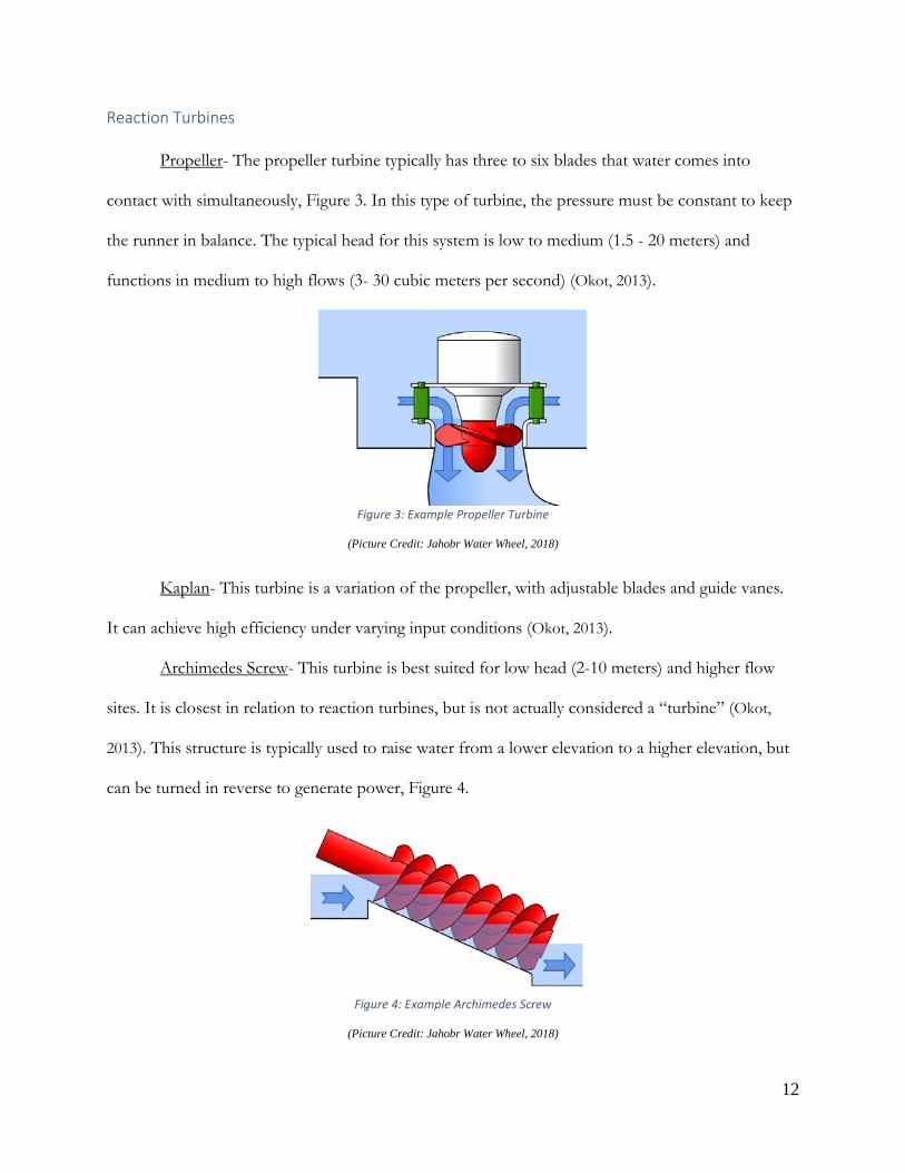
Propeller- The propeller turbine typically has three to six blades that water comes into

contact with simultaneously, Figure 3. In this type of turbine, the pressure must be constant to keep

the runner in balance. The typical head for this system is low to medium (1.5 - 20 meters) and

functions in medium to high flows (3- 30 cubic meters per second) (Okot, 2013).

Figure 3: Example Propeller Turbine


Kaplan- This turbine is a variation of the propeller, with adjustable blades and guide vanes.

It can achieve high efficiency under varying input conditions (Okot, 2013).

Archimedes Screw- This turbine is best suited for low head (2-10 meters) and higher flow

sites. It is closest in relation to reaction turbines, but is not actually considered a “turbine” (Okot,

2013). This structure is typically used to raise water from a lower elevation to a higher elevation, but

can be turned in reverse to generate power, Figure 4.

Figure 4: Example Archimedes Screw


13

Waterwheels

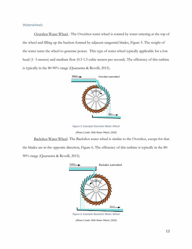
Overshot Water Wheel - The Overshot water wheel is rotated by water entering at the top of

the wheel and filling up the buckets formed by adjacent tangential blades, Figure 5. The weight of

the water turns the wheel to generate power. This type of water wheel typically applicable for a low

head (1- 5 meters) and medium flow (0.3-1.5 cubic meters per second). The efficiency of this turbine

is typically in the 80-90% range (Quarantra & Revelli, 2015).

Figure 5: Example Overshot Water Wheel

(Photo Credit: Wiki Water Wheel, 2018)

Backshot Water Wheel- The Backshot water wheel is similar to the Overshot, except for that

the blades are in the opposite direction, Figure 6. The efficiency of this turbine is typically in the 80-

90% range (Quarantra & Revelli, 2015).

Figure 6: Example Backshot Water Wheel

(Photo Credit: Wiki Water Wheel, 2018)

14

2.3 Pico-Hydro Power Generation

Pico-hydro is a term to describe hydropower systems that output less than 5 kilowatts

(Williamson et al, 2014). Several turbines have already been designed and tested for pico-hydro

applications. Pico-hydro is of increased interest for off-grid applications in low-income areas. Pico-

hydro systems are typically low cost because significant construction is not needed in order to

implement the systems (Williamson et al., 2014). These systems also have minimal environmental

impacts because they are managed by the consumer and are not interfering with animal habitats or

emitting pollutants (Williamson et al., 2014). In Nepal, 300 pico-hydro systems are producing

electricity and an additional 900 are used for mechanical power (Cobb & Sharp, 2013). Some

downsides to pico-hydro include the need for specific site conditions, such as heavy rainfall or a

nearby water source.

Several studies have shown both Pelton wheels and Turgo turbines are utilized in pico-hydro

systems. These two turbines are good for this application because they have high efficiencies in a

wide range of conditions. Turgo turbines in particular have been shown to perform better than

Pelton wheels in higher flow rates and lower heads (Cobb & Sharp, 2013). In testing, Turgo turbines

were able to perform at over 80% efficiency, which is “quite good” for pico-hydro (Cobb & Sharp,

2013). The different angles and striking points of the water are factors that can influence the

efficiency of the turbine.

2.4 Electrical Components

For pico-hydro turbines in a rainwater catchment system, the flow can be both variable in

magnitude and intermittent, additionally the amount of power being generated at any given time is

small. This creates challenges for generating electricity from a pico-hydro rainwater energy

harvesting system. There are two common generator types that are ideal for ultra-low hydropower:

15

squirrel cage induction generators and direct current synchronous generators (Zhou & Deng, 2017).

Overall, permanent magnet synchronous generators are superior at handling a wider range of speeds

because they can still produce power through a range of speeds and squirrel cage induction

generators are superior in that they require little maintenance (Zhou & Deng, 2017). For small scale

electricity generation, another option for electricity generation is to use a permanent magnet DC

motor as a generator. Permanent magnet DC motors operate at a range of input powers to provide a

range of output powers. When they are run in reverse by rotating the shaft they can convert the

input mechanical power to electrical power. The ability to generate power at a range of input

conditions make permanent magnet DC motors a good option for a generator. Ratings for DC

motors are given in terms of the stall torque and the maximum RPM. At the stall torque the RPM

will be 0 and at the maximum RPMs the torque will be zero, the maximum power extracted from a

DC motor is at half the stall torque and half the max rated RPMs (Understanding D.C. Motor

Characteristics, 2018). This is shown in the Figure 7, below. Theoretically, the same should be true

in reverse and if the motor is used as a generator and half of the maximum RPM and torque is input

to the motor it should output the most power.

Figure 7: DC Motor Rotational Speed vs Torque

16

2.5 Energy Harvesting from Rainwater for Household Systems

Household hydropower systems provide energy by extracting power from high head water

pipes. Kanth, Ashwani, Sharma (2012) explored a theoretical household system that would combine

energy harvesting with water catchment from rooftops for individual buildings located in regions

where typhoons or heavy rains are common. The gravitational potential energy of the rainwater

would be converted to kinetic energy. The stream of water would strike a turbine to cause the

turbine to rotate. The turbine would be connected to a generator to produce electrical power. Kanth

et al. would use the gutters on the roof to funnel the rainwater from the rooftop to a storage tank

located at ground level. The turbine would be placed in the downspout and above the storage tank,

locations can vary depending on the type of the turbine used. For a roof area of 185 meters squared,

and an average rainfall of 43 centimeters per year, the system was calculated to produce 1.5 kilowatt-

hours per year. If the system was located in the rainiest locations on Earth, it would be able to

produce 48 kilowatt-hours per year (Kanth et al., 2012), this is equivalent to about 8,640 phone

charges. In comparison to other forms of energy generation this is actually minimal, however for

rainy climates with little electricity access the technology can be used to supplement other forms of

energy.

An experiment done by Bhargav, Ratna Kishore, Anbuudayasankar, Balaji (2016) harvested

the gravitational potential energy of water in an overhead tank at the top of a three-story apartment

building before the water entered a tap in an intermediate system. The assembly consisted of a 0.25

meter diameter pipe, a storage tank 15 meters above the tap, and a 135 millimeter turbine. An

impulse-motor cooling fan was used as a turbine and was contained in an external enclosure, Figure

8. A shaft, supported by bearings within the case of the turbine, was coupled with a 12 Volt

permanent magnet direct current (DC) generator. When the system was running the generator

17

produced 1.5 Watts. The advantages of this generator include minimal transmission losses because

the energy was converted immediately to DC rather than AC power.

Figure 8: Assembly of Turbine

(Photo Credit: Bhargav et al, 2015)

18

3 Design and Construction

The following section outlines the design concepts for the overall system and calculations

required to estimate the power output of this proposed system. Construction of the prototype is

discussed. The section also details the preliminary tests completed in order to arrive at specific

design decisions.

3.1 System Components, Initial Design, and Project Scope

The system we are proposing is a dual purpose power generation and water collection. The

eight components in the system and their main functions are outlined below:

1. Roof: must provide a smooth surface for water to flow down to the gutter,

2. Gutter: must be large enough to collect a significant portion of the water off the roof and

angled to ensure the flow of water to the downspout,

3. Gutter-to-downspout connector: must direct the water towards the center of the downspout

to minimize friction with the walls, and create a smooth stream of water,

4. Downspout: must be large enough to contain the water from the gutter and avoid

backfilling,

5. Turbine/enclosure: placed at the outlet of the downspout to ensure the stream of water will

strike and rotate the turbine,

6. Electrical components/enclosure: attached to the turbine shaft to produce electrical power;

the enclosure will ensure the components stay dry in the wet environment,

7. Filtration system: purify the water so that it is safe to drink, and

8. Holding tank: store collected rainwater for future use.

19

Figure 9 depicts a drawing of our initial design. The rainwater will be collected from the roof via the

gutter system that will run along the perimeter of the house. The water will be directed into the

downspout that leads into an enclosure with a turbine. After the water flows through the turbine, it

is collected in a tank beneath the system where it will be stored and can be filtered for drinking

water.

Figure 9: Initial Design

Project Scope

There are three components outside the scope of the project: the roof, the holding tank, and

the filtration system. The system proposed begins with the roof. The roofs on low-income families’

homes in Liberia are made of corrugated metal. An example image of a corrugated roof is below in

Figure 10.

.

20

Figure 10: Home in Liberia with Corrugated Roof

(Photo Credit: Google Street View, 2018)

The corrugated metal will provide a smooth surface for the water to flow down to the gutter.

The roofs are also slightly angled to ensure the flow of water. The material and design of the roofs

in the proposed location are already satisfactory for the system. Furthermore, the system is intended

for low-income families and should not induce extraneous costs. Therefore, we will not be

considering redesigning the roof for our system.

The scope of our projects is primarily focused on the conversion of rainwater into

energy. Therefore, the project will focus on the gutter and downspout sub-system, the turbine and

its enclosure, and the electrical components and their enclosure. We will not work to design the final

components of the system, the holding tank and filtration system, as filtration techniques and

holding tank have been thoroughly researched in other projects. In summary, we will work to create

a well-designed system that includes a gutter, downspout, and rainwater energy generator.

3.2 Initial Power Calculation

Prior to making any design decisions, we calculated the maximum potential power

harvestable from the system using theoretical values. We considered the system under two different

scenarios: water flowing through a filled downspout and free falling water. In the first scenario, the

21

downspout would have a nozzle at the very end immediately before the turbine to direct the stream

of water on the turbine blades. The small nozzle area would cause the downspout to backfill and

provide a pressure head. In the second scenario, the rainwater from the gutter would be directed to

the center of the downspout with no backup. The downspout would not be filled and the water

would ideally not touch the sides of the downspout. We considered both scenarios to determine

which one would be the most beneficial and produce the most power.

The first scenario involves a nozzle at the end of the downspout. The small nozzle area

would cause the downspout to backfill as rain continues to enter the downspout. If the downspout

is filled, however, there will be frictional losses in the form of Equation 1:

ℎ𝑙𝑙 = 𝑓𝑓 �𝐿𝐿𝐷𝐷��

𝑉𝑉2

2𝑔𝑔� (1)

(Munson, Okiishi, Huebsch, & Rothmayer, 2013, pg. 428)

Where:

ℎ1 = 𝐻𝐻𝐻𝐻𝐻𝐻𝐻𝐻 𝐿𝐿𝐿𝐿𝐿𝐿𝐿𝐿 (𝑚𝑚)

𝑓𝑓 = 𝐹𝐹𝐹𝐹𝐹𝐹𝐹𝐹𝐹𝐹𝐹𝐹𝐿𝐿𝐹𝐹 𝐹𝐹𝐻𝐻𝐹𝐹𝐹𝐹𝐿𝐿𝐹𝐹 (𝑢𝑢𝐹𝐹𝐹𝐹𝐹𝐹𝑢𝑢𝐻𝐻𝐿𝐿𝐿𝐿)

𝑢𝑢 = 𝐿𝐿𝐻𝐻𝐹𝐹𝑔𝑔𝐹𝐹ℎ 𝐿𝐿𝑓𝑓 𝐹𝐹ℎ𝐻𝐻 𝑃𝑃𝐹𝐹𝑃𝑃𝐻𝐻 (𝑚𝑚)

𝐷𝐷 = 𝐷𝐷𝐹𝐹𝐻𝐻𝑚𝑚𝐻𝐻𝐹𝐹𝐻𝐻𝐹𝐹 𝐿𝐿𝑓𝑓 𝑃𝑃𝐹𝐹𝑃𝑃𝐻𝐻 (𝑚𝑚)

𝑉𝑉 = 𝑉𝑉𝐻𝐻𝑢𝑢𝐿𝐿𝐹𝐹𝐹𝐹𝐹𝐹𝑉𝑉 𝐸𝐸𝐸𝐸𝐹𝐹𝐹𝐹𝐹𝐹𝐹𝐹𝑔𝑔 𝐹𝐹ℎ𝐻𝐻 𝑃𝑃𝐹𝐹𝑃𝑃𝐻𝐻 �𝑚𝑚𝐿𝐿�

𝑔𝑔 = 𝐺𝐺𝐹𝐹𝐻𝐻𝐺𝐺𝐹𝐹𝐹𝐹𝑉𝑉 �𝑚𝑚2

𝐿𝐿�

The frictional losses will decrease the maximum velocity that exits the nozzle, and will

therefore lower the power production and the RPM. Because the system is small-scale, the goal was

to minimize losses as much as possible, therefore a nozzle at the end of the downspout and

backfilling the downspout would not be beneficial. Rather, designing the downspout so that the

22

water falls in a single stream down the center of the downspout to strike the blade will help to

enhance the performance of the system.

In the second scenario, the water would be directed to the center of the downspout to avoid

frictional losses. The calculations outlined below estimate the power production from a 20

centimeter diameter Pelton wheel for the case of free-falling water during the heaviest rain. The

Pelton wheel was chosen for the calculations because the equations are well-developed and easily

accessible.

The first step was to calculate the flow rate of the water off of the roof based on the roof

area and rainfall intensity. The theoretical roof area used for the project was 5 meters in length by 3

meters in depth. Thus the roof area is 15 meters squared. The maximum rainfall intensity was based

on 2 year characterization of rainfall data in Liberia. The maximum intensity is 272.40 millimeters

per hour and occurs for 0.10 hour (6 minutes) (Golder Associates, 2012). The volumetric flow rate

of the water entering the pipe is determined by Equation 2:

𝑄𝑄 = 𝐴𝐴 ∗ 𝐼𝐼 (2)

Where:

𝑄𝑄 = 𝐹𝐹𝑢𝑢𝐿𝐿𝐹𝐹 𝑅𝑅𝐻𝐻𝐹𝐹𝐻𝐻 �𝑚𝑚3

𝐿𝐿�

𝐴𝐴 = 𝐴𝐴𝐻𝐻𝐴𝐴𝑢𝑢𝐿𝐿𝐹𝐹𝐻𝐻𝐻𝐻 𝐴𝐴𝐹𝐹𝐻𝐻𝐻𝐻 (𝑚𝑚3)

𝐼𝐼 = 𝑅𝑅𝐻𝐻𝐹𝐹𝐹𝐹𝑓𝑓𝐻𝐻𝑢𝑢𝑢𝑢 𝐼𝐼𝐹𝐹𝐹𝐹𝐻𝐻𝐹𝐹𝐿𝐿𝐹𝐹𝐹𝐹𝑉𝑉 �𝑚𝑚ℎ𝐹𝐹�

𝑄𝑄 = 15 ∗ 0.2724 ∗ �1

3600�

𝑄𝑄 = 0.001135 �𝑚𝑚3

𝐿𝐿� 𝐿𝐿𝐹𝐹 �17.99

𝑔𝑔𝐻𝐻𝑢𝑢𝑢𝑢𝐿𝐿𝐹𝐹𝐿𝐿𝑚𝑚𝐹𝐹𝐹𝐹𝑢𝑢𝐹𝐹𝐻𝐻

�

23

Before entering the gutter, the water has kinetic energy coming off of the roof. For the

purposes of this power estimation, we will assume any of the kinetic energy of the water flowing off

the roof is dissipated on impact with the gutter and therefore we do not consider this initial velocity.

The velocity of the water in the gutter before it enters the downspout was determined using open

channel flow calculations and is given by Equation 3:

𝑉𝑉 =�𝑘𝑘 �𝐴𝐴𝑃𝑃�

2 3⁄�ℎ𝑢𝑢 �

1 2⁄�

𝐹𝐹 (3)

(Munson et al, 2013, pg. 568)

Where:

𝑉𝑉 = 𝑉𝑉𝐻𝐻𝑢𝑢𝐿𝐿𝐹𝐹𝐹𝐹𝐹𝐹𝑉𝑉 𝐿𝐿𝑓𝑓 𝑊𝑊𝐻𝐻𝐹𝐹𝐻𝐻𝐹𝐹 𝐹𝐹𝐹𝐹 𝐺𝐺𝑢𝑢𝐹𝐹𝐹𝐹𝐻𝐻𝐹𝐹 �𝑚𝑚𝐿𝐿�

𝐴𝐴 = 𝐶𝐶𝐹𝐹𝐿𝐿𝐿𝐿𝐿𝐿 − 𝑆𝑆𝐻𝐻𝐹𝐹𝐹𝐹𝐹𝐹𝐿𝐿𝐹𝐹𝐻𝐻𝑢𝑢 𝐴𝐴𝐹𝐹𝐻𝐻𝐻𝐻 𝐿𝐿𝑓𝑓 𝐶𝐶ℎ𝐻𝐻𝐹𝐹𝐹𝐹𝐻𝐻𝑢𝑢 (𝑚𝑚2)

𝑃𝑃 = 𝑊𝑊𝐻𝐻𝐹𝐹𝐹𝐹𝐻𝐻𝐻𝐻 𝑃𝑃𝐻𝐻𝐹𝐹𝐹𝐹𝑚𝑚𝐻𝐻𝐹𝐹𝐻𝐻𝐹𝐹 (𝑚𝑚)

ℎ = 𝐷𝐷𝐹𝐹𝑓𝑓𝑓𝑓𝐻𝐻𝐹𝐹𝐻𝐻𝐹𝐹𝐹𝐹𝐻𝐻 𝐹𝐹𝐹𝐹 𝐻𝐻𝐻𝐻𝐹𝐹𝑔𝑔ℎ𝐹𝐹 𝐵𝐵𝐻𝐻𝐹𝐹𝐹𝐹𝐻𝐻𝐻𝐻𝐹𝐹 𝑇𝑇𝐿𝐿𝑃𝑃 𝐻𝐻𝐹𝐹𝐻𝐻 𝐵𝐵𝐿𝐿𝐹𝐹𝐹𝐹𝐿𝐿𝑚𝑚 𝐿𝐿𝑓𝑓 𝐺𝐺𝑢𝑢𝐹𝐹𝐹𝐹𝐻𝐻𝐹𝐹 (𝑢𝑢𝐹𝐹𝐹𝐹𝐹𝐹𝑢𝑢𝐻𝐻𝐿𝐿𝐿𝐿)

𝑢𝑢 = 𝐿𝐿𝐻𝐻𝐹𝐹𝑔𝑔𝐹𝐹ℎ 𝐿𝐿𝑓𝑓 𝐺𝐺𝑢𝑢𝐹𝐹𝐹𝐹𝐻𝐻𝐹𝐹 (𝑚𝑚)

𝐹𝐹 = 𝑀𝑀𝐻𝐻𝐹𝐹𝐹𝐹𝐹𝐹𝐹𝐹𝑔𝑔 𝐶𝐶𝐿𝐿𝐻𝐻𝑓𝑓𝑓𝑓𝐹𝐹𝐹𝐹𝐻𝐻𝐹𝐹𝐹𝐹 �𝐿𝐿

𝑚𝑚13�

𝑘𝑘 = 𝐶𝐶𝐿𝐿𝐹𝐹𝐺𝐺𝐻𝐻𝐹𝐹𝐿𝐿𝐹𝐹𝐿𝐿𝐹𝐹 𝐹𝐹𝐻𝐻𝐹𝐹𝐹𝐹𝐿𝐿𝐹𝐹 (𝑘𝑘 = 1 𝑓𝑓𝐿𝐿𝐹𝐹 𝑆𝑆𝐼𝐼 𝑈𝑈𝐹𝐹𝐹𝐹𝐹𝐹𝐿𝐿)

A standard half round painted aluminum gutter from Home Depot will be used as a

theoretical gutter for the purposes of the calculations. The gutter has a diameter of 12.7 centimeters

(5 inches). The length of the gutter is the length of the roof: 5 meters. A typical gutter slope is 1%

(Still & Thomas, 2002; SMACNA, 2012). The manning resistance coefficient, n, is 0.014 for painted

metal (Munson et al., 2013, pg. 569). We assumed that the filled height was about 75% of the radius

24

in order to perform the calculations, so the height was 4.76 centimeters. The area and wetted

perimeter can be found by calculating the circular segment area and arc length of the circular

segment filled by the water, respectively, shown in Figure 11, to find the arc length we need to know

theta, calculated using Equation 4.

Figure 11: Circular Segment Filled by Water

𝜃𝜃 = 2 ∗ arccos �𝐹𝐹 − ℎℎ

� (4)

𝜃𝜃 = 2 ∗ arccos �5.7 − 4.28

5.7�

𝜃𝜃 = 2.63 𝐹𝐹𝐻𝐻𝐻𝐻𝐹𝐹𝐻𝐻𝐹𝐹𝐿𝐿

Knowing theta, we could find the arc length, which is the wetted perimeter using Equation 5:

𝑃𝑃 = 𝐹𝐹 ∗ 𝜃𝜃 (5)

𝑃𝑃 = 6.35 ∗ 2.63

𝑃𝑃 = 16.74 𝐹𝐹𝑚𝑚 = 0.1674 𝑚𝑚

The circular segment area is given by Equation 6:

𝐴𝐴 = �𝐹𝐹2(𝜃𝜃 − 𝐿𝐿𝐹𝐹𝐹𝐹𝜃𝜃)

2� (6)

25

𝐴𝐴 = 4.3 ∗ 10−3 𝑚𝑚2

Therefore, the velocity is:

𝑉𝑉 =[1 �4.3 ∗ 10−3

0.1503 �2 3⁄

(0.01)1 2⁄ ]

0.014

𝑉𝑉 = 0.622𝑚𝑚𝐿𝐿

To be conservative in our estimates, and because the open channel flow calculations proved

the velocity of the water the gutter to be small, we neglected this velocity and only considered the

potential energy of water at the top of the downspout. Assuming all of the potential energy from the

height of the water is converted into kinetic energy, the velocity of the water exiting the pipe is

found using Equation 7:

𝑉𝑉 = �2𝑔𝑔ℎ (7)

Where:


𝑔𝑔 = 𝐺𝐺𝐹𝐹𝐻𝐻𝐺𝐺𝐹𝐹𝐹𝐹𝑉𝑉 �𝑚𝑚2

𝐿𝐿�

ℎ = 𝐻𝐻𝐻𝐻𝐹𝐹𝑔𝑔ℎ𝐹𝐹 𝐿𝐿𝑓𝑓 𝐹𝐹ℎ𝐻𝐻 𝐺𝐺𝑢𝑢𝐹𝐹𝐹𝐹𝐻𝐻𝐹𝐹 (𝑚𝑚)

The height of the roof is estimated to be 3 meters above the ground due to standard ceiling

heights. Thus the velocity of water exiting the downspout is:

𝑉𝑉 = √2 ∗ 9.8 ∗ 3

𝑉𝑉 = 7.67 𝑚𝑚𝐿𝐿

26

The maximum power for a Pelton wheel is modeled by Equation 8:

𝑃𝑃 = 𝜌𝜌𝑄𝑄𝑈𝑈(𝑈𝑈 − 𝑉𝑉)(1 − 𝐹𝐹𝐿𝐿𝐿𝐿𝑐𝑐) (8)

(Munson et al., 2013, pg. 700)

Where:

𝑃𝑃 = 𝑃𝑃𝐿𝐿𝐹𝐹𝐻𝐻𝐹𝐹 (𝑊𝑊)

𝜌𝜌 = 𝐷𝐷𝐻𝐻𝐹𝐹𝐿𝐿𝐹𝐹𝐹𝐹𝑉𝑉 𝐿𝐿𝑓𝑓 𝑊𝑊𝐻𝐻𝐹𝐹𝐻𝐻𝐹𝐹 �𝑘𝑘𝑔𝑔𝑚𝑚3�


𝐿𝐿�

𝑈𝑈 = 𝐵𝐵𝑢𝑢𝐻𝐻𝐻𝐻𝐻𝐻 𝑆𝑆𝑃𝑃𝐻𝐻𝐻𝐻𝐻𝐻 �𝑚𝑚𝐿𝐿�


𝑐𝑐 = 𝐸𝐸𝐸𝐸𝐹𝐹𝐹𝐹 𝐴𝐴𝐹𝐹𝑔𝑔𝑢𝑢𝐻𝐻 𝐿𝐿𝑓𝑓 𝐹𝐹ℎ𝐻𝐻 𝐵𝐵𝑢𝑢𝐻𝐻𝐻𝐻𝐻𝐻 (𝐷𝐷𝐻𝐻𝑔𝑔𝐹𝐹𝐻𝐻𝐻𝐻𝐿𝐿)

Beta is the exit angle of the blade. Ideally, the water would exit at a 180 degree angle.

However, this is not physically possible as the exiting water would collide with the entering water. It

has been determined that an exit angle of 165 degrees is optimal (Munson et al., 2013, pg. 700).

U is the blade speed. At maximum power, the optimal blade speed is one half of the water

velocity (Munson et al., 2013, pg. 700). Replacing U with ½ V, the power produced by the Pelton

wheel can be calculated in Equation 9:

P = ρQ�V2��

V2� − V� (1− cosβ) (9)

𝑃𝑃 = 1000 ∗ 0.001135 ∗ �7.67

2� ∗ ��

7.672� − 7.67� ∗ (1 − cos(165))

𝑃𝑃 = 32.82 𝑊𝑊

27

The above calculations estimated the maximum potential power for a theoretical house with

a roof area of 3 meters by 5 meters and a height of 3 meters at a rainfall intensity of 272 millimeters

per hour. The maximum potential power for the theoretical house is plotted against the rainfall

intensity in Figure 12.

The same calculations were completed to estimate the maximum potential power we would

be able to produce in laboratory testing. The prototype system has a height of 2 meters (prototype

discussed in Section 3.3). The maximum potential power for both the theoretical house and our

prototyped system is plotted against the rainfall intensity in Figure 12. As a note, the maximum flow

rate from the hose is 8 GPM, corresponding to a rainfall intensity of 120 millimeters per hour.

Therefore, the maximum potential power output from the turbine in our prototype is approximately

10 Watts.

Figure 12: Theoretical Power Output of the Turbine vs Rainfall Intensity

A 272 millimeter per hour rainfall intensity would last six minutes, from this peak storm the

energy harvested would be calculated in Equation 10:

28

𝐸𝐸 = 𝑃𝑃 ∗ 𝐹𝐹 (10)

Where:

𝐸𝐸 = 𝐸𝐸𝐹𝐹𝐻𝐻𝐹𝐹𝑔𝑔𝑉𝑉 (𝐽𝐽)

𝑃𝑃 = 𝑃𝑃𝐿𝐿𝐹𝐹𝐻𝐻𝐹𝐹 (𝑊𝑊)

𝐹𝐹 = 𝑇𝑇𝐹𝐹𝑚𝑚𝐻𝐻 𝐹𝐹ℎ𝐻𝐻𝐹𝐹 𝐹𝐹ℎ𝐻𝐻 𝑆𝑆𝐹𝐹𝐹𝐹𝐿𝐿𝑚𝑚 𝐿𝐿𝐻𝐻𝐿𝐿𝐹𝐹𝐿𝐿 (𝐿𝐿𝐻𝐻𝐹𝐹𝐿𝐿𝐹𝐹𝐻𝐻𝐿𝐿)

𝐸𝐸 = 32.82 ∗ 360

𝐸𝐸 = 11815 𝐽𝐽

A cell phone battery charge requires about 20,000 Joules (assuming cell phone battery holds

5.45 watt hours) and lighting one LED for one hour requires 36,000 Joules (assuming 10 W light

bulb), the energy can be put into perspective by Equation 11 and Equation 12:

𝑁𝑁𝑢𝑢𝑚𝑚𝑁𝑁𝐻𝐻𝐹𝐹 𝐿𝐿𝑓𝑓 𝐶𝐶𝐻𝐻𝑢𝑢𝑢𝑢 𝑃𝑃ℎ𝐿𝐿𝐹𝐹𝐻𝐻𝐿𝐿 = 𝐸𝐸𝐹𝐹𝐻𝐻𝐹𝐹𝑔𝑔𝑉𝑉

𝐸𝐸𝐹𝐹𝐻𝐻𝐹𝐹𝑔𝑔𝑉𝑉 𝑃𝑃𝐻𝐻𝐹𝐹 𝐶𝐶ℎ𝐻𝐻𝐹𝐹𝑔𝑔𝐻𝐻 (11)

𝑁𝑁𝑢𝑢𝑚𝑚𝑁𝑁𝐻𝐻𝐹𝐹 𝐿𝐿𝑓𝑓 𝐶𝐶𝐻𝐻𝑢𝑢𝑢𝑢 𝑃𝑃ℎ𝐿𝐿𝐹𝐹𝐻𝐻𝐿𝐿 = 1181520000

𝑁𝑁𝑢𝑢𝑚𝑚𝑁𝑁𝐻𝐻𝐹𝐹 𝐿𝐿𝑓𝑓 𝐶𝐶𝐻𝐻𝑢𝑢𝑢𝑢 𝑃𝑃ℎ𝐿𝐿𝐹𝐹𝐻𝐻𝐿𝐿 = 0.59

𝑁𝑁𝑢𝑢𝑚𝑚𝑁𝑁𝐻𝐻𝐹𝐹 𝐿𝐿𝑓𝑓 𝐿𝐿𝐹𝐹𝑔𝑔ℎ𝐹𝐹 𝐻𝐻𝐿𝐿𝑢𝑢𝐹𝐹𝐿𝐿 = 𝐸𝐸𝐹𝐹𝐻𝐻𝐹𝐹𝑔𝑔𝑉𝑉

𝐸𝐸𝐹𝐹𝐻𝐻𝐹𝐹𝑔𝑔𝑉𝑉 𝑃𝑃𝐻𝐻𝐹𝐹 𝐶𝐶ℎ𝐻𝐻𝐹𝐹𝑔𝑔𝐻𝐻 (12)

𝑁𝑁𝑢𝑢𝑚𝑚𝑁𝑁𝐻𝐻𝐹𝐹 𝐿𝐿𝑓𝑓 𝐿𝐿𝐹𝐹𝑔𝑔ℎ𝐹𝐹 𝐻𝐻𝐿𝐿𝑢𝑢𝐹𝐹𝐿𝐿 = 1181536000

𝑁𝑁𝑢𝑢𝑚𝑚𝑁𝑁𝐻𝐻𝐹𝐹 𝐿𝐿𝑓𝑓 𝐿𝐿𝐹𝐹𝑔𝑔ℎ𝐹𝐹 𝐻𝐻𝐿𝐿𝑢𝑢𝐹𝐹𝐿𝐿 = 0.33

Over the course of the day the rainfall intensity would vary, this is just the cell phone charges

and light-hours from a short 6 minute storm. Depending on the rainfall more power may be

generated over the course of an entire day.

29

3.3 Prototype for Testing Structure

In order to test individual components of our design during the design and preliminary

testing process, and to test the system as a whole, we built a testing structure to fix to the testing

tank, Figure 13. We constructed the frame from Aluminum 80/20s that was secured with C clamps

to the testing tank. The length of the structure is 1.8 meters (6 feet), with a height of 1.2 meters (4

feet), and a width of 1 meter (3.3 feet). A 1.8 meter (6 feet) wooden 2 by 4 was installed to the top of

the tank with L brackets to support the gutter.

Figure 13: Design of Test Structure

We purchased a 10 foot vinyl gutter from Home Depot and cut it in half to ensure the gutter

would fit on the wooden 2 by 4 and hang within the length of the tank. The now 5 foot piece of

gutter was installed to the wooden 2 by 4 using vinyl hidden hangers, also purchased from Home

Depot, to mimic how the gutter would be installed on a typical home, Figure 16.

30

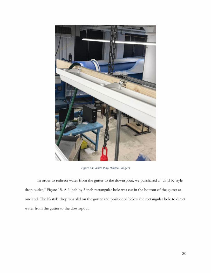
Figure 14: White Vinyl Hidden Hangers

In order to redirect water from the gutter to the downspout, we purchased a “vinyl K-style

drop outlet,” Figure 15. A 6 inch by 3 inch rectangular hole was cut in the bottom of the gutter at

one end. The K-style drop was slid on the gutter and positioned below the rectangular hole to direct

water from the gutter to the downspout.

31

Figure 15: Assembled Gutter

(Photo Credit: Home Depot)

Downspout elbow connectors, straight connectors, and 3 15 inch straight downspout pieces

were purchased to test different downspout orientations, described in Section 3.4. These pieces

could be assembled and attached to the rectangular opening of the K-style drop outlet. Gutter end

caps were installed on both ends of the gutter to prevent water from exiting at either end and sealed

with the tri-polymer based sealant, SealerMate. The final design of the gutter/downspout subsystem

is described in Section 3.4.

Inside the tank, we placed a stand to hold the turbines for testing. Attached to the stand was

a separate, watertight compartment for the electronics to sit in. The turbine stand was made by laser

cutting acrylic pieces and using acrylic adhesive for assembly. Plastic ball bearings, with stainless steel

balls, held a keyed shaft in place. The bearings were chosen due to their ability to operate well in wet

environments, and their resistance to corrosion. A keyed shaft was chosen to make it simple to test

different turbines because the reverse key could be implemented in all of our turbine designs. Shaft

collars were used to keep the shaft in place. An exploded view with all of these components is

shown in Figure 16 below.

32

Figure 16: Exploded View of Turbine Stand

The aluminum frame to hold the gutter and the turbine stand were used to conduct tests for

the gutter/downspout sub-system, the turbine, and the electrical components to aid in our final

design decisions. Detailed descriptions of our decision process, pre-testing, and final design choices

are described in the following sections.

3.4 Gutter and Downspout Sub-System

The gutter and downspout sub-system includes the gutter, the gutter-to-downspout

connector, and the downspout itself. This section outlines the calculations, considerations, and tests

to determine the gutter sizing and slope, the preferred gutter-to-downspout connection, and the

downspout design to develop a final design for the sub-system.

Gutter Sizing and Slope

Sizing the gutter to contain the water coming off the roof was the first step of designing this

sub-system. The gutter sizing calculations were completed using two approaches. The first approach

determines the velocity and projection of the water coming off the roof to determine the necessary

width of the gutter.

33

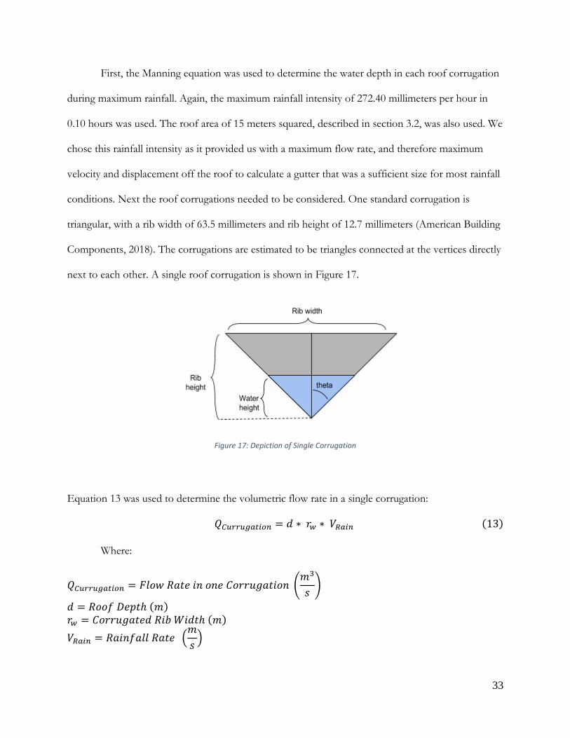
First, the Manning equation was used to determine the water depth in each roof corrugation

during maximum rainfall. Again, the maximum rainfall intensity of 272.40 millimeters per hour in

0.10 hours was used. The roof area of 15 meters squared, described in section 3.2, was also used. We

chose this rainfall intensity as it provided us with a maximum flow rate, and therefore maximum

velocity and displacement off the roof to calculate a gutter that was a sufficient size for most rainfall

conditions. Next the roof corrugations needed to be considered. One standard corrugation is

triangular, with a rib width of 63.5 millimeters and rib height of 12.7 millimeters (American Building

Components, 2018). The corrugations are estimated to be triangles connected at the vertices directly

next to each other. A single roof corrugation is shown in Figure 17.

Figure 17: Depiction of Single Corrugation

Equation 13 was used to determine the volumetric flow rate in a single corrugation:

𝑄𝑄𝐶𝐶𝐶𝐶𝐶𝐶𝐶𝐶𝐶𝐶𝐶𝐶𝐶𝐶𝐶𝐶𝐶𝐶𝐶𝐶𝐶𝐶 = 𝐻𝐻 ∗ 𝐹𝐹𝑤𝑤 ∗ 𝑉𝑉𝑅𝑅𝐶𝐶𝐶𝐶𝐶𝐶 (13)

Where:

𝑄𝑄𝐶𝐶𝐶𝐶𝐶𝐶𝐶𝐶𝐶𝐶𝐶𝐶𝐶𝐶𝐶𝐶𝐶𝐶𝐶𝐶𝐶𝐶 = 𝐹𝐹𝑢𝑢𝐿𝐿𝐹𝐹 𝑅𝑅𝐻𝐻𝐹𝐹𝐻𝐻 𝐹𝐹𝐹𝐹 𝐿𝐿𝐹𝐹𝐻𝐻 𝐶𝐶𝐿𝐿𝐹𝐹𝐹𝐹𝑢𝑢𝑔𝑔𝐻𝐻𝐹𝐹𝐹𝐹𝐿𝐿𝐹𝐹 �𝑚𝑚3

𝐿𝐿�

𝐻𝐻 = 𝑅𝑅𝐿𝐿𝐿𝐿𝑓𝑓 𝐷𝐷𝐻𝐻𝑃𝑃𝐹𝐹ℎ (𝑚𝑚) 𝐹𝐹𝑤𝑤 = 𝐶𝐶𝐿𝐿𝐹𝐹𝐹𝐹𝑢𝑢𝑔𝑔𝐻𝐻𝐹𝐹𝐻𝐻𝐻𝐻 𝑅𝑅𝐹𝐹𝑁𝑁 𝑊𝑊𝐹𝐹𝐻𝐻𝐹𝐹ℎ (𝑚𝑚)

𝑉𝑉𝑅𝑅𝐶𝐶𝐶𝐶𝐶𝐶 = 𝑅𝑅𝐻𝐻𝐹𝐹𝐹𝐹𝑓𝑓𝐻𝐻𝑢𝑢𝑢𝑢 𝑅𝑅𝐻𝐻𝐹𝐹𝐻𝐻 �𝑚𝑚𝐿𝐿�

34

𝑄𝑄𝐶𝐶𝐶𝐶𝐶𝐶𝐶𝐶𝐶𝐶𝐶𝐶𝐶𝐶𝐶𝐶𝐶𝐶𝐶𝐶𝐶𝐶 = 3 ∗ 0.0635 ∗ 0.27240 ∗ (1

3600)

𝑄𝑄𝐶𝐶𝐶𝐶𝐶𝐶𝐶𝐶𝐶𝐶𝐶𝐶𝐶𝐶𝐶𝐶𝐶𝐶𝐶𝐶𝐶𝐶 = 14.415 ∗ 10−6 �𝑚𝑚3

𝐿𝐿�

Next the Manning Equation for open channel flow was used to determine if the maximum

intensity of rainfall would overflow the gutter, Equation 14:

𝑄𝑄 = �𝑘𝑘𝐹𝐹� ∗ 𝐴𝐴 ∗ 𝑅𝑅ℎ

23 ∗ 𝑆𝑆𝐶𝐶

12 (14)

𝑅𝑅ℎ = 𝐴𝐴𝑃𝑃

(Munson et al., 2013, pg. 568-570)

Where:

𝐹𝐹 = 𝑀𝑀𝐻𝐻𝐹𝐹𝐹𝐹𝐹𝐹𝐹𝐹𝑔𝑔 𝑅𝑅𝐻𝐻𝐿𝐿𝐹𝐹𝐿𝐿𝐹𝐹𝐻𝐻𝐹𝐹𝐹𝐹𝐻𝐻 𝐶𝐶𝐿𝐿𝐻𝐻𝑓𝑓𝑓𝑓𝐹𝐹𝐹𝐹𝐹𝐹𝐻𝐻𝐹𝐹𝐹𝐹 �𝐿𝐿

𝑚𝑚13�

𝑘𝑘 = 𝐶𝐶𝐿𝐿𝐹𝐹𝐺𝐺𝐻𝐻𝐹𝐹𝐿𝐿𝐹𝐹𝐿𝐿𝐹𝐹 𝐹𝐹𝐻𝐻𝐹𝐹𝐹𝐹𝐿𝐿𝐹𝐹, 1 𝐹𝐹𝑓𝑓 𝑆𝑆𝐼𝐼 𝑈𝑈𝐹𝐹𝐹𝐹𝐹𝐹𝐿𝐿 𝐻𝐻𝐹𝐹𝐻𝐻 𝑈𝑈𝐿𝐿𝐻𝐻𝐻𝐻 (𝑢𝑢𝐹𝐹𝐹𝐹𝐹𝐹𝑢𝑢𝐻𝐻𝐿𝐿𝐿𝐿) 𝐴𝐴 = 𝐶𝐶𝐹𝐹𝐿𝐿𝐿𝐿𝐿𝐿 𝑆𝑆𝐻𝐻𝐹𝐹𝐹𝐹𝐹𝐹𝐿𝐿𝐹𝐹𝐻𝐻𝑢𝑢 𝐹𝐹𝑢𝑢𝐿𝐿𝐹𝐹 𝐴𝐴𝐹𝐹𝐻𝐻𝐻𝐻 (𝑚𝑚2) 𝑅𝑅ℎ = 𝐻𝐻𝑉𝑉𝐻𝐻𝐹𝐹𝐻𝐻𝑢𝑢𝑢𝑢𝐹𝐹𝐹𝐹 𝑅𝑅𝐻𝐻𝐻𝐻𝐹𝐹𝑢𝑢𝐿𝐿 (𝑚𝑚) 𝑃𝑃 = 𝑊𝑊𝐻𝐻𝐹𝐹𝐹𝐹𝐻𝐻𝐻𝐻 𝑃𝑃𝐻𝐻𝐹𝐹𝐹𝐹𝑚𝑚𝐻𝐻𝐹𝐹𝐻𝐻𝐹𝐹 (𝑚𝑚) 𝑆𝑆𝐶𝐶 = 𝑆𝑆𝑢𝑢𝐿𝐿𝑃𝑃𝐻𝐻 𝐿𝐿𝑓𝑓 𝐹𝐹ℎ𝐻𝐻 𝐶𝐶ℎ𝐻𝐻𝐹𝐹𝐹𝐹𝐻𝐻𝑢𝑢 (𝑢𝑢𝐹𝐹𝐹𝐹𝐹𝐹𝑢𝑢𝐻𝐻𝐿𝐿𝐿𝐿)

The goal was to use the Manning Equation to determine the height of water in the channel.

The geometry of the corrugations was considered in order to solve for the area as a function of

height of water in each corrugation. Knowing the rib height and the rib width, theta was determined

to be 68.2 degrees. The area of water for the Manning Equation is the cross-sectional area of water

in the gutter. Therefore, cross sectional area of water in the gutter as a function of height was

calculated by Equation 15:

𝐴𝐴 = ℎ2 ∗ 𝐹𝐹𝐻𝐻𝐹𝐹𝜃𝜃 (15)

Where:

𝐴𝐴 = 𝐶𝐶𝐹𝐹𝐿𝐿𝐿𝐿𝐿𝐿 𝑆𝑆𝐻𝐻𝐹𝐹𝐹𝐹𝐹𝐹𝐿𝐿𝐹𝐹𝐻𝐻𝑢𝑢 𝑊𝑊𝐻𝐻𝐹𝐹𝐻𝐻𝐹𝐹 𝐴𝐴𝐹𝐹𝐻𝐻𝐻𝐻 (𝑚𝑚2)

ℎ = 𝑊𝑊𝐻𝐻𝐹𝐹𝐻𝐻𝐹𝐹 𝐻𝐻𝐻𝐻𝐹𝐹𝑔𝑔ℎ𝐹𝐹 (𝑚𝑚)

35

The hydraulic radius in terms of height was calculated by Equation 16:

𝑅𝑅ℎ = ℎ ∗ sin𝜃𝜃 ∗ 0.5 (16)

The manning resistance coefficient, n, is 0.022 for corrugated metal and k is 1 because SI

units are being used (Munson et al., 2013, pg. 569). The Architectural Sheet Metal Manual states that

a low roof slope is 3 inch for every 12 inch of roof (75 millimeters for 305 millimeters), so the slope,

S0, is 0.25 (SMACNA, 2012). We chose a low slope because the images of Liberian homes that we

found appeared to have low sloping roofs. Now the Manning Equation could be solved for height

so that the height of water in the corrugations could be determined from the geometry of the

corrugations and the flowrate of rain. The Manning Equation, Equation 17, solved for height is:

ℎ = �𝑄𝑄 ∗ 𝐹𝐹

𝑘𝑘 ∗ 𝐹𝐹𝐻𝐻𝐹𝐹𝜃𝜃 ∗ (𝐿𝐿𝐹𝐹𝐹𝐹𝜃𝜃)23 ∗ 𝑆𝑆𝐶𝐶

12�

12

(17)

ℎ = ((14.415 ∗ 10−6) ∗ 0.022

𝑘𝑘 ∗ tan(68.2) ∗ [sin (68.2)]23 ∗ (0.25)

12

)12

ℎ = 3.425 𝑚𝑚𝐹𝐹𝑢𝑢𝑢𝑢𝐹𝐹𝑚𝑚𝐻𝐻𝐹𝐹𝐻𝐻𝐹𝐹𝐿𝐿

The original geometry of the corrugated roof has a rib height of 12.7 millimeters, so this

suggests that in full flow the corrugations of the roof will not be overflowed by the rain because the

corrugations would only need 3.425 millimeters in rib height to handle 272.4 millimeter per hour of

water.

Using the determined height of water in the gutter, the velocity of the water in the

corrugations could be determined by Equation 18:

𝑉𝑉 = 𝑄𝑄𝐴𝐴

(18)

36

Where:

𝑉𝑉 = 𝑉𝑉𝐻𝐻𝑢𝑢𝐿𝐿𝐹𝐹𝐹𝐹𝐹𝐹𝑉𝑉 𝐿𝐿𝑓𝑓 𝑊𝑊𝐻𝐻𝐹𝐹𝐻𝐻𝐹𝐹 �𝑚𝑚𝐿𝐿�

𝑄𝑄 = 𝑉𝑉𝐿𝐿𝑢𝑢𝑢𝑢𝑚𝑚𝐻𝐻𝐹𝐹𝐹𝐹𝐹𝐹𝐹𝐹 𝐹𝐹𝑢𝑢𝐿𝐿𝐹𝐹 𝑅𝑅𝐻𝐻𝐹𝐹𝐻𝐻 𝐹𝐹𝐹𝐹 𝑆𝑆𝐹𝐹𝐹𝐹𝑔𝑔𝑢𝑢𝐻𝐻 𝐶𝐶𝐿𝐿𝐹𝐹𝐹𝐹𝑢𝑢𝑔𝑔𝐻𝐻𝐹𝐹𝐹𝐹𝐿𝐿𝐹𝐹 (𝑚𝑚3)

𝐴𝐴 = 𝐶𝐶𝐹𝐹𝐿𝐿𝐿𝐿𝐿𝐿 𝑆𝑆𝐻𝐻𝐹𝐹𝐹𝐹𝐹𝐹𝐿𝐿𝐹𝐹𝐻𝐻𝑢𝑢 𝐴𝐴𝐹𝐹𝐻𝐻𝐻𝐻 𝐿𝐿𝑓𝑓 𝑊𝑊𝐻𝐻𝐹𝐹𝐻𝐻𝐹𝐹 𝐹𝐹𝐹𝐹 𝐶𝐶𝐿𝐿𝐹𝐹𝐹𝐹𝑢𝑢𝑔𝑔𝐻𝐻𝐹𝐹𝐹𝐹𝐿𝐿𝐹𝐹 (𝐴𝐴 = ℎ2 ∗ 𝐹𝐹𝐻𝐻𝐹𝐹𝜃𝜃)(𝑚𝑚2)

𝑉𝑉 =(14.415 ∗ 10−6)

[(0.003425)2 ∗ tan(68.2)]

𝑉𝑉 = 0.491 𝑚𝑚𝐿𝐿

The last step was to use the velocity coming off of the roof to determine the distance the

gutter should be placed horizontally from the roof. The displacement was determined using the

basic kinematics equations. First the time spent falling was found, and then the horizontal

displacement was found. Figure 18, illustrates the velocity components.

Figure 18: Velocity Components

The vertical displacement from the edge of the roof to the top of the gutter was estimated to

be 5 centimeters. As previously explained the roof has a slope of 3 inches down for every 12 inches

in length, this corresponds to a 14.04 degree slope. Knowing the overall velocity component, the

vertical component could be determined and the time it would take for the water to fall 5

centimeters could be found using Equation 19 and Equation 20:

∆𝑉𝑉 = 𝐺𝐺𝑦𝑦𝐹𝐹 ∗ (0.5) ∗ 𝑔𝑔𝐹𝐹2 (19)

37

𝐺𝐺𝑦𝑦 = 𝐺𝐺 ∗ 𝐿𝐿𝐹𝐹𝐹𝐹𝜃𝜃 (20)

Where:

∆𝑉𝑉 = 𝑉𝑉𝐻𝐻𝐹𝐹𝐹𝐹𝐹𝐹𝐹𝐹𝐻𝐻𝑢𝑢 𝐷𝐷𝐹𝐹𝐿𝐿𝑃𝑃𝑢𝑢𝐻𝐻𝐹𝐹𝐻𝐻𝑚𝑚𝐻𝐻𝐹𝐹𝐹𝐹 (𝑚𝑚)

𝐺𝐺 = 𝑉𝑉𝐻𝐻𝑢𝑢𝐿𝐿𝐹𝐹𝐹𝐹𝐹𝐹𝑉𝑉 𝐿𝐿𝑓𝑓 𝑊𝑊𝐻𝐻𝐹𝐹𝐻𝐻𝐹𝐹 𝐹𝐹𝐹𝐹 𝐶𝐶𝐿𝐿𝐹𝐹𝐹𝐹𝑢𝑢𝑔𝑔𝐻𝐻𝐹𝐹𝐹𝐹𝐿𝐿𝐹𝐹 𝐶𝐶𝐿𝐿𝑚𝑚𝐹𝐹𝐹𝐹𝑔𝑔 𝑂𝑂𝑓𝑓𝑓𝑓 𝐹𝐹ℎ𝐻𝐻 𝑅𝑅𝐿𝐿𝐿𝐿𝑓𝑓 �𝑚𝑚𝐿𝐿�

𝐺𝐺𝑦𝑦𝐹𝐹 = 𝑉𝑉𝐻𝐻𝐹𝐹𝐹𝐹𝐹𝐹𝐹𝐹𝐻𝐻𝑢𝑢 𝐶𝐶𝐿𝐿𝑚𝑚𝑃𝑃𝐿𝐿𝐹𝐹𝐻𝐻𝐹𝐹𝐹𝐹 𝐿𝐿𝑓𝑓 𝑉𝑉𝐻𝐻𝑢𝑢𝐿𝐿𝐹𝐹𝐹𝐹𝐹𝐹𝑉𝑉 �𝑚𝑚𝐿𝐿�

𝐹𝐹 = 𝑇𝑇𝐹𝐹𝑚𝑚𝐻𝐻 (𝐿𝐿)

𝑔𝑔 = 𝐺𝐺𝐹𝐹𝐻𝐻𝐺𝐺𝐹𝐹𝐹𝐹𝑉𝑉 �𝑚𝑚𝐿𝐿2�

𝜃𝜃 = 𝐴𝐴𝐹𝐹𝑔𝑔𝑢𝑢𝐻𝐻 𝐿𝐿𝑓𝑓 𝑅𝑅𝐿𝐿𝐿𝐿𝑓𝑓 (𝐻𝐻𝐻𝐻𝑔𝑔𝐹𝐹𝐻𝐻𝐻𝐻𝐿𝐿)

0.05 = 𝐹𝐹 ∗ sin(14.04) ∗ (0.5) ∗ (9.8) ∗ 𝐹𝐹2

𝐹𝐹 = 0.099 𝐿𝐿𝐻𝐻𝐹𝐹𝐿𝐿𝐹𝐹𝐻𝐻𝐿𝐿

Last, determining the displacement from the roof was calculated by Equation 21 and Equation 22:

∆𝐸𝐸 = 𝐺𝐺𝑥𝑥𝐹𝐹 (21)

𝐺𝐺𝑥𝑥 = 𝐺𝐺𝐹𝐹𝐿𝐿𝐿𝐿𝜃𝜃 (22)

Where:

∆𝐸𝐸 = 𝑉𝑉𝐻𝐻𝐹𝐹𝐹𝐹𝐹𝐹𝐹𝐹𝐻𝐻𝑢𝑢 𝐷𝐷𝐹𝐹𝐿𝐿𝑃𝑃𝑢𝑢𝐻𝐻𝐹𝐹𝐻𝐻𝑚𝑚𝐻𝐻𝐹𝐹𝐹𝐹 (𝑚𝑚)

𝐺𝐺 = 𝑉𝑉𝐻𝐻𝑢𝑢𝐿𝐿𝐹𝐹𝐹𝐹𝐹𝐹𝑉𝑉 𝐿𝐿𝑓𝑓 𝑊𝑊𝐻𝐻𝐹𝐹𝐻𝐻𝐹𝐹 𝐹𝐹𝐹𝐹 𝐶𝐶𝐿𝐿𝐹𝐹𝐹𝐹𝑢𝑢𝑔𝑔𝐻𝐻𝐹𝐹𝐹𝐹𝐿𝐿𝐹𝐹 𝐶𝐶𝐿𝐿𝑚𝑚𝐹𝐹𝐹𝐹𝑔𝑔 𝑂𝑂𝑓𝑓𝑓𝑓 𝐹𝐹ℎ𝐻𝐻 𝑅𝑅𝐿𝐿𝐿𝐿𝑓𝑓 �𝑚𝑚𝐿𝐿�

𝐺𝐺𝑥𝑥 = 𝑉𝑉𝐻𝐻𝐹𝐹𝐹𝐹𝐹𝐹𝐹𝐹𝐻𝐻𝑢𝑢 𝐶𝐶𝐿𝐿𝑚𝑚𝑃𝑃𝐿𝐿𝐹𝐹𝐻𝐻𝐹𝐹𝐹𝐹 𝐿𝐿𝑓𝑓 𝑉𝑉𝐻𝐻𝑢𝑢𝐿𝐿𝐹𝐹𝐹𝐹𝐹𝐹𝑉𝑉 �𝑚𝑚𝐿𝐿�

𝐹𝐹 = 𝑇𝑇𝐹𝐹𝑚𝑚𝐻𝐻 (𝐿𝐿)

𝜃𝜃 = 𝐴𝐴𝐹𝐹𝑔𝑔𝑢𝑢𝐻𝐻 𝐿𝐿𝑓𝑓 𝑅𝑅𝐿𝐿𝐿𝐿𝑓𝑓 (𝐻𝐻𝐻𝐻𝑔𝑔𝐹𝐹𝐻𝐻𝐻𝐻𝐿𝐿)

38

∆𝐸𝐸 = (0.099) ∗ (0.491) ∗ cos(14.03)

∆𝐸𝐸 = 4.72 𝐹𝐹𝐻𝐻𝐹𝐹𝐹𝐹𝐹𝐹𝑚𝑚𝐻𝐻𝐹𝐹𝐻𝐻𝐹𝐹𝐿𝐿

This means in the maximum rainfall, the gutter should be able to catch rain that is displaced

4.72 centimeters from the edge of the roof. If this is taken to be the distance from the center of the

gutter to the edge of the gutter than the gutter diameter should be twice the distance found, or 9.43

centimeters (approximately 3.71 inches) wide.

The limitation of this method of gutter sizing is it considers the width needed but does not

calculate the depth of the gutter needed. For this, and as a way to verify the previous results, we

turned to gutter sizing equations from the seventh edition of the Architectural Sheet Metal Manual

by the Sheet Metal and Air Conditioning Contractors' National Association, SMACNA (SMACNA,

2012). The solution of the equations provides for the width of rectangular and half round level

gutters. The formulas have been experimentally verified by the National Institute of Standards and

Technology and have been derived for use with English units only. Graphs of the equations in both

English and metric units can be found in Appendix A.

For rectangular gutters, Equation 23 was used:

𝑊𝑊 = 0.0106𝑀𝑀−4 7⁄ ∗ 𝐿𝐿3 28⁄ ∗ �𝐼𝐼𝐴𝐴5 14⁄ � (23)

Where:

𝑊𝑊 = 𝑊𝑊𝐹𝐹𝐻𝐻𝐹𝐹ℎ 𝐿𝐿𝑓𝑓 𝐹𝐹ℎ𝐻𝐻 𝐺𝐺𝑢𝑢𝐹𝐹𝐹𝐹𝐻𝐻𝐹𝐹 (𝑓𝑓𝐹𝐹)

𝑀𝑀 = 𝑅𝑅𝐻𝐻𝐹𝐹𝐹𝐹𝐿𝐿 𝐿𝐿𝑓𝑓 𝐷𝐷𝐻𝐻𝑃𝑃𝐹𝐹ℎ (𝐷𝐷)𝐹𝐹𝐿𝐿 𝑊𝑊𝐹𝐹𝐻𝐻𝐹𝐹ℎ 𝐿𝐿𝑓𝑓 𝐺𝐺𝑢𝑢𝐹𝐹𝐹𝐹𝐻𝐻𝐹𝐹,𝐷𝐷𝑊𝑊

(𝑢𝑢𝐹𝐹𝐹𝐹𝐹𝐹𝑢𝑢𝐻𝐻𝐿𝐿𝐿𝐿)

𝐿𝐿 = 𝐿𝐿𝐻𝐻𝐹𝐹𝑔𝑔𝐹𝐹ℎ 𝐿𝐿𝑓𝑓 𝐺𝐺𝑢𝑢𝐹𝐹𝐹𝐹𝐻𝐻𝐹𝐹 (𝑓𝑓𝐹𝐹)

39

𝐼𝐼 = 𝑅𝑅𝐻𝐻𝐹𝐹𝐹𝐹𝑓𝑓𝐻𝐻𝑢𝑢𝑢𝑢 𝐼𝐼𝐹𝐹𝐹𝐹𝐻𝐻𝐹𝐹𝐿𝐿𝐹𝐹𝐹𝐹𝑉𝑉 �𝐹𝐹𝐹𝐹ℎ𝐹𝐹�

𝐴𝐴 = 𝐴𝐴𝐹𝐹𝐻𝐻𝐻𝐻 𝐹𝐹𝐿𝐿 𝑁𝑁𝐻𝐻 𝐷𝐷𝐹𝐹𝐻𝐻𝐹𝐹𝐹𝐹𝐻𝐻𝐻𝐻 (𝑓𝑓𝐹𝐹2)

For the ratio of the depth to width, we chose a standard value of 0.75. For the purpose of

our calculations, we again used a rectangular roof with a length of 5 meters (approximately 16 feet)

and a width of 3 meters (approximately 10 feet). Therefore, the length of the gutter is 5 meters, or

approximately 16 feet. A roof slope of 3 inches in 12 inches, or 75 millimeters in 305 millimeters,

was used again. The highest rainfall intensity of 272.40 millimeters per hour is approximately 10.7

inches per hour. The area is dependent on the roof length, width, and pitch was calculated by

Equation 24:

𝐴𝐴 = 𝐿𝐿 ∗ 𝑊𝑊 ∗ 𝑃𝑃 (24)

Where:

𝐴𝐴 = 𝐴𝐴𝐻𝐻𝐴𝐴𝑢𝑢𝐿𝐿𝐹𝐹𝐻𝐻𝐻𝐻 𝐴𝐴𝐹𝐹𝐻𝐻𝐻𝐻 (𝑓𝑓𝐹𝐹2)

𝐿𝐿 = 𝐿𝐿𝐻𝐻𝐹𝐹𝑔𝑔𝐹𝐹ℎ 𝐿𝐿𝑓𝑓 𝐹𝐹ℎ𝐻𝐻 𝑅𝑅𝐿𝐿𝐿𝐿𝑓𝑓 (𝑓𝑓𝐹𝐹)

𝑊𝑊 = 𝑊𝑊𝐹𝐹𝐻𝐻𝐹𝐹ℎ 𝐿𝐿𝑓𝑓 𝐹𝐹ℎ𝐻𝐻 𝑅𝑅𝐿𝐿𝐿𝐿𝑓𝑓 (𝑓𝑓𝐹𝐹)

𝑃𝑃 = 𝑃𝑃𝐹𝐹𝐹𝐹𝐹𝐹ℎ 𝐹𝐹𝐻𝐻𝐹𝐹𝐹𝐹𝐿𝐿𝐹𝐹 (𝑢𝑢𝐹𝐹𝐹𝐹𝐹𝐹𝑢𝑢𝐻𝐻𝐿𝐿𝐿𝐿)

The plane roof area must be multiplied by a pitch factor because steeper roofs are more

likely to “catch” rain as the wind blows the rain onto the roof. For our slope, the pitch factor is 1.00,

as shown in Table 1.

40

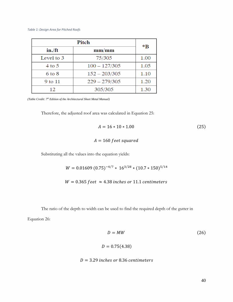
Table 1: Design Area for Pitched Roofs

(Table Credit: 7th Edition of the Architectural Sheet Metal Manual)

Therefore, the adjusted roof area was calculated in Equation 25:

𝐴𝐴 = 16 ∗ 10 ∗ 1.00 (25)

𝐴𝐴 = 160 𝑓𝑓𝐻𝐻𝐻𝐻𝐹𝐹 𝐿𝐿𝑠𝑠𝑢𝑢𝐻𝐻𝐹𝐹𝐻𝐻𝐻𝐻

Substituting all the values into the equation yields:

𝑊𝑊 = 0.01609 (0.75)−4 7⁄ ∗ 163 28⁄ ∗ (10.7 ∗ 150)5 14⁄

𝑊𝑊 = 0.365 𝑓𝑓𝐻𝐻𝐻𝐻𝐹𝐹 ≈ 4.38 𝐹𝐹𝐹𝐹𝐹𝐹ℎ𝐻𝐻𝐿𝐿 𝐿𝐿𝐹𝐹 11.1 𝐹𝐹𝐻𝐻𝐹𝐹𝐹𝐹𝐹𝐹𝑚𝑚𝐻𝐻𝐹𝐹𝐻𝐻𝐹𝐹𝐿𝐿

The ratio of the depth to width can be used to find the required depth of the gutter in

Equation 26:

𝐷𝐷 = 𝑀𝑀𝑊𝑊 (26)

𝐷𝐷 = 0.75(4.38)

𝐷𝐷 = 3.29 𝐹𝐹𝐹𝐹𝐹𝐹ℎ𝐻𝐻𝐿𝐿 𝐿𝐿𝐹𝐹 8.36 𝐹𝐹𝐻𝐻𝐹𝐹𝐹𝐹𝐹𝐹𝑚𝑚𝐻𝐻𝐹𝐹𝐻𝐻𝐹𝐹𝐿𝐿

41

For half-round gutters, only the rainfall intensity and roof area contribute to determining the

width in Equation 27:

𝑊𝑊 = 0.0182(𝐼𝐼𝐴𝐴)2 5⁄ (27)

𝑊𝑊 = 0.0182(10.72 ∗ 160)2 5⁄

𝑊𝑊 = 0.358 𝑓𝑓𝐻𝐻𝐻𝐻𝐹𝐹 ≈ 4.30 𝐹𝐹𝐹𝐹𝐹𝐹ℎ𝐻𝐻𝐿𝐿 𝐿𝐿𝐹𝐹 10.9 𝐹𝐹𝐻𝐻𝐹𝐹𝐹𝐹𝐹𝐹𝑚𝑚𝐻𝐻𝐹𝐹𝐻𝐻𝐹𝐹𝐿𝐿

Both methods of calculations provided results in similar ranges. Therefore, in order to

contain the maximum amount of rain during the heaviest of storms, the gutter width should be

between 8.36 centimeters (3.29 inches) and 10.9 centimeters (4.30 inches) depending on the

geometry. The necessary depth of the gutter is dependent on the shape of the gutter.

The prior equations are valid for level gutters. However, sloped gutters are more efficient in

terms of capturing and conveying the water. A sloped gutter is able to serve a larger roof area than a

level gutter of the same size (SMACNA, 2012). Typical grades for gutters range between 0.5% and

2% (Still & Thomas, 2002; SMACNA, 2012). A medium grade of 1% is the most efficient in terms

of water capture and conveyance (Still & Thomas, 2002). To size a half-round sloped gutter, the

Architectural Sheet Metal Manual is used again. Table 2 displays the maximum roof area to be

served by different sized half-round gutters installed at varying slopes. A 1% grade equates to a slope

of ⅛ inch per foot. The roof areas to be served by each size gutter and slope is based on a rainfall

intensity of 1 inch per hour. Dividing the roof areas in the ⅛ inch per foot column by our maximum

rainfall intensity of 10.7 inches per hour, yields the actual roof area to be served by the gutter.

42

Table 2: Sloped Half-Round Gutter Capacity

(Table Credit: 7th Edition of the Architectural Sheet Metal Manual)

Therefore, a roof area of 150 square feet, or 14 meters squared, could be served by two 3-

inch half-round gutters installed at a slope of ⅛ inch per foot. One gutter could be installed on

either side of the house for a home with the common gable style roof. Alternatively, if the home has

a mono-pitch, or shed-like roof, a single 4-inch half-round gutter installed at a slope of ⅛ inch per

foot could serve the entire roof.

For the purposes of our prototype, we purchased a gutter that was easily available to us at a

local home improvement store. The purchased gutter is a 10-foot K-shaped vinyl gutter that is 3

inches wide and 3.25 inches deep. The gutter was cut in half to a length of 5 feet so that it would fit

over the tank and on our 80/20 stand. The 5-foot section of gutter was installed onto the 2 by 4

piece of wood using the same installation hooks one would use to attach the gutter to a house. One

of the 80/20s spanning across the tank was moved down 0.6 inches from the top of the vertical

80/20s to create the desired 1% grade.

43

Gutter-to-Downspout Connection Types

There are several different ways to connect a gutter to a downspout. The most common type

of connection involves a funnel-like component on the gutter that connects to the downspout. Most

of the time elbow connectors and short lengths of downspouts are attached to the funnel

connection to lead the downspout back to the side of the house to be supported, Figure 19.

However, the downspout may not require the elbow connections if it can be supported by a

structure other than the side of the house, Figure 20. Another option we came across was simply an

open end of a gutter that emptied into a vessel for collecting the rainwater, Figure 21.

Figure 19: Elbow Connectors and Short Lengths of Downspout

(Photo Credit: USA Gutters, 2018)

44

Figure 20: Straight Downspout

(Photo Credit: DZ/DG, 2018)

Figure 21: Open End Gutter

(Photo Credit: Eggleston Farkas Architects)

45

Gutter-to-Downspout Connection Tests

To determine the most suitable gutter-to-downspout connection, we conducted preliminary

testing of five different types of connections: vertical downspout (Figure 22), bent downspout

(Figure 23), vertical downspout with 1.4 centimeter and 1.1 centimeter funnels placed at the top of

the downspout (Figure 24), and the open end gutter. The connection ideally should produce a single

stream, or at least a primary stream, of water to strike the turbine. If the water disperses too much,

the stream would not be powerful enough to start the turbine. The hose was placed in the gutter and

each connection was evaluated at four different flow rates: 8 GPM, 6 GPM, 4 GPM, and 2 GPM.

After initial tests, the open end gutter was immediately eliminated because the position of the stream

changed drastically for each flow rate. This would not be feasible for the system as the turbine

would have to be moved frequently to adjust to the position of the stream.

Figure 22: Vertical Downspout

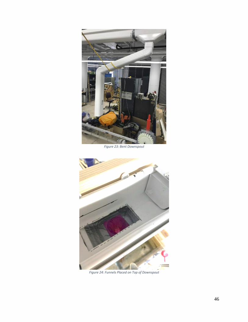
46

Figure 23: Bent Downspout

Figure 24: Funnels Placed on Top of Downspout

47

In order to evaluate and estimate the size of the streams coming out of the downspout for

each different connection, we drew measurements on a piece of cardboard. The cardboard was

covered in plastic and held behind the stream. We took photos of the streams to compare stream

sizes for each connection type at each flow rate. The stream for the plain vertical downspout was

very inconsistent and spread out, as seen in Figure 25a. The stream for the bent downspout (Figure

25b) was better, but still not ideal as it was very wide and changed positions often. The streams from

the two funnels and vertical downspout were the best as there was only a single stream that stayed in

the same location throughout testing (Figure 25c & d).

Figure 25: Stream Size for (a) Vertical Downspout, (b) Bent Downspout, (c) 1.4 centimeter Funnel, (d) 1.1 cm Funnel

Adding a funnel to the top of the downspout was the most favorable option. During the

testing to estimate the stream size, the gutter would fill up quickly because the funnels were not large

enough to allow the full flow of water through the opening. We estimated the necessary diameter of

a funnel opening by matching the cross-sectional area of the water in the gutter without any funnel

48

attached to the area of a circular opening. The estimated cross-sectional area of the water in the

gutter was 9.68 centimeters squared (1.5 inches squared) at the hose’s maximum flow rate of 8

GPM. A diameter of 3.51 centimeters (1.38 inches) would produce a circular area of the same size.

In order to confidently determine the appropriate opening size of the funnel, we conducted

an experiment. Our goal was to have an opening that would be small enough to produce some back-

up in the gutter at every flow – as funnels produce smoother, more consistent stream when there is

some pressure head – but the funnel also needed to be large enough that the gutter would not

overflow in high intensity range.

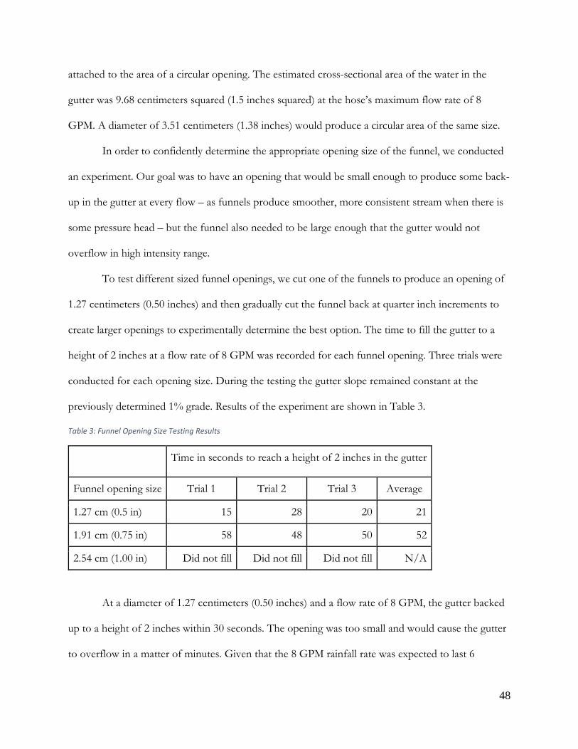
To test different sized funnel openings, we cut one of the funnels to produce an opening of

1.27 centimeters (0.50 inches) and then gradually cut the funnel back at quarter inch increments to

create larger openings to experimentally determine the best option. The time to fill the gutter to a

height of 2 inches at a flow rate of 8 GPM was recorded for each funnel opening. Three trials were

conducted for each opening size. During the testing the gutter slope remained constant at the

previously determined 1% grade. Results of the experiment are shown in Table 3.

Table 3: Funnel Opening Size Testing Results

Time in seconds to reach a height of 2 inches in the gutter

Funnel opening size Trial 1 Trial 2 Trial 3 Average

1.27 cm (0.5 in) 15 28 20 21

1.91 cm (0.75 in) 58 48 50 52

2.54 cm (1.00 in) Did not fill Did not fill Did not fill N/A

At a diameter of 1.27 centimeters (0.50 inches) and a flow rate of 8 GPM, the gutter backed

up to a height of 2 inches within 30 seconds. The opening was too small and would cause the gutter

to overflow in a matter of minutes. Given that the 8 GPM rainfall rate was expected to last 6

49

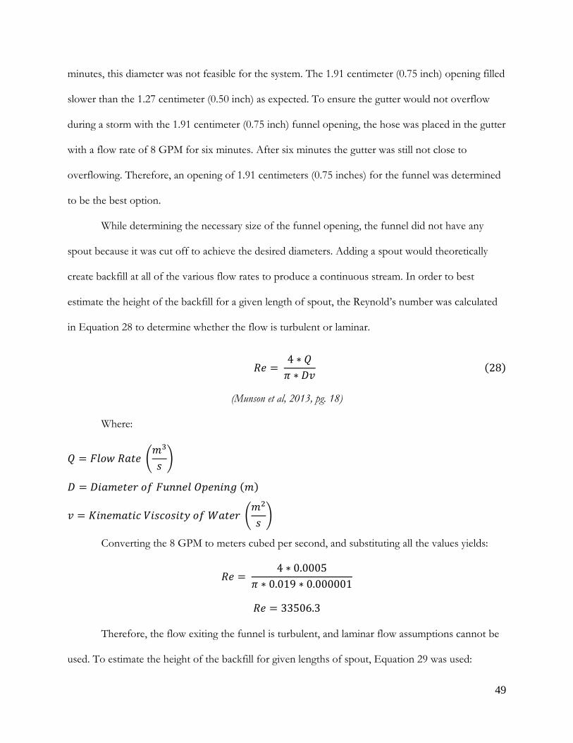
minutes, this diameter was not feasible for the system. The 1.91 centimeter (0.75 inch) opening filled

slower than the 1.27 centimeter (0.50 inch) as expected. To ensure the gutter would not overflow

during a storm with the 1.91 centimeter (0.75 inch) funnel opening, the hose was placed in the gutter

with a flow rate of 8 GPM for six minutes. After six minutes the gutter was still not close to

overflowing. Therefore, an opening of 1.91 centimeters (0.75 inches) for the funnel was determined

to be the best option.

While determining the necessary size of the funnel opening, the funnel did not have any

spout because it was cut off to achieve the desired diameters. Adding a spout would theoretically

create backfill at all of the various flow rates to produce a continuous stream. In order to best

estimate the height of the backfill for a given length of spout, the Reynold’s number was calculated

in Equation 28 to determine whether the flow is turbulent or laminar.

𝑅𝑅𝐻𝐻 = 4 ∗ 𝑄𝑄𝜋𝜋 ∗ 𝐷𝐷𝐺𝐺

(28)

(Munson et al, 2013, pg. 18)

Where:


𝐿𝐿�

𝐷𝐷 = 𝐷𝐷𝐹𝐹𝐻𝐻𝑚𝑚𝐻𝐻𝐹𝐹𝐻𝐻𝐹𝐹 𝐿𝐿𝑓𝑓 𝐹𝐹𝑢𝑢𝐹𝐹𝐹𝐹𝐻𝐻𝑢𝑢 𝑂𝑂𝑃𝑃𝐻𝐻𝐹𝐹𝐹𝐹𝐹𝐹𝑔𝑔 (𝑚𝑚)

𝐺𝐺 = 𝐾𝐾𝐹𝐹𝐹𝐹𝐻𝐻𝑚𝑚𝐻𝐻𝐹𝐹𝐹𝐹𝐹𝐹 𝑉𝑉𝐹𝐹𝐿𝐿𝐹𝐹𝐿𝐿𝐿𝐿𝐹𝐹𝐹𝐹𝑉𝑉 𝐿𝐿𝑓𝑓 𝑊𝑊𝐻𝐻𝐹𝐹𝐻𝐻𝐹𝐹 �𝑚𝑚2

𝐿𝐿�

Converting the 8 GPM to meters cubed per second, and substituting all the values yields:

𝑅𝑅𝐻𝐻 = 4 ∗ 0.0005

𝜋𝜋 ∗ 0.019 ∗ 0.000001

𝑅𝑅𝐻𝐻 = 33506.3

Therefore, the flow exiting the funnel is turbulent, and laminar flow assumptions cannot be

used. To estimate the height of the backfill for given lengths of spout, Equation 29 was used:

50

𝐿𝐿′ + 𝐿𝐿 = 𝐺𝐺2

2 ∗ 𝑔𝑔∗ �𝑘𝑘 + 𝑓𝑓 ∗

𝐿𝐿𝐷𝐷� (29)

Where:

𝐿𝐿′ = 𝑇𝑇ℎ𝐻𝐻 𝐻𝐻𝐻𝐻𝐹𝐹𝑔𝑔ℎ𝐹𝐹 𝐿𝐿𝑓𝑓 𝐹𝐹ℎ𝐻𝐻 𝑊𝑊𝐻𝐻𝐹𝐹𝐻𝐻𝐹𝐹 𝐴𝐴𝑁𝑁𝐿𝐿𝐺𝐺𝐻𝐻 𝐹𝐹ℎ𝐻𝐻 𝐸𝐸𝐹𝐹𝐹𝐹𝐹𝐹𝐻𝐻𝐹𝐹𝐹𝐹𝐻𝐻 𝐿𝐿𝑓𝑓 𝐹𝐹ℎ𝐻𝐻 𝑆𝑆𝑃𝑃𝐿𝐿𝑢𝑢𝐹𝐹 (𝑚𝑚)

𝐿𝐿 = 𝐿𝐿𝐻𝐻𝐹𝐹𝑔𝑔𝐹𝐹ℎ 𝐿𝐿𝑓𝑓 𝐹𝐹ℎ𝐻𝐻 𝑆𝑆𝑃𝑃𝐿𝐿𝑢𝑢𝐹𝐹 (𝑚𝑚)

𝐺𝐺 = 𝑉𝑉𝐻𝐻𝑢𝑢𝐿𝐿𝐹𝐹𝐹𝐹𝐹𝐹𝑉𝑉 𝐿𝐿𝑓𝑓 𝑊𝑊𝐻𝐻𝐹𝐹𝐻𝐻𝐹𝐹 𝐸𝐸𝐸𝐸𝐹𝐹𝐹𝐹𝐹𝐹𝐹𝐹𝐹𝐹𝑔𝑔 𝐹𝐹ℎ𝐻𝐻 𝑆𝑆𝑃𝑃𝐿𝐿𝑢𝑢𝐹𝐹 �𝑚𝑚𝐿𝐿�

𝑔𝑔 = 𝐺𝐺𝐹𝐹𝐻𝐻𝐺𝐺𝐹𝐹𝐹𝐹𝑉𝑉 �𝑚𝑚𝐿𝐿2�

𝑘𝑘 = 𝑀𝑀𝐹𝐹𝐹𝐹𝐿𝐿𝐹𝐹 𝐻𝐻𝐻𝐻𝐻𝐻𝐻𝐻 𝐿𝐿𝐿𝐿𝐿𝐿𝐿𝐿𝐻𝐻𝐿𝐿 𝐶𝐶𝐿𝐿𝐻𝐻𝑓𝑓𝑓𝑓𝐹𝐹𝐹𝐹𝐹𝐹𝐻𝐻𝐹𝐹𝐹𝐹 (𝑢𝑢𝐹𝐹𝐹𝐹𝐹𝐹𝑢𝑢𝐻𝐻𝐿𝐿𝐿𝐿)

𝑓𝑓 = 𝐹𝐹𝐹𝐹𝐹𝐹𝐹𝐹𝐹𝐹𝐹𝐹𝐿𝐿𝐹𝐹 𝐹𝐹𝐻𝐻𝐹𝐹𝐹𝐹𝐿𝐿𝐹𝐹 (𝑢𝑢𝐹𝐹𝐹𝐹𝐹𝐹𝑢𝑢𝐻𝐻𝐿𝐿𝐿𝐿)

𝐷𝐷 = 𝐷𝐷𝐹𝐹𝐻𝐻𝑚𝑚𝐻𝐻𝐹𝐹𝐻𝐻𝐹𝐹 𝐿𝐿𝑓𝑓 𝐹𝐹𝑢𝑢𝐹𝐹𝐹𝐹𝐻𝐻𝑢𝑢 𝑂𝑂𝑃𝑃𝐻𝐻𝐹𝐹𝐹𝐹𝐹𝐹𝑔𝑔 (𝑚𝑚)

In the equation, L’ + L represent the pressure head. The majority of the losses stem from

the minor loss coefficient. Based on the geometry of the funnel, an approximate value of k is 0.25

(Munson et al., 2013, pg. 434). Using the Reynold’s number and the Moody chart, an approximate

friction factor is 0.025 (Munson et al., 2013, pg. 430). The velocity exiting the funnel is determined

by using V = Q/A. The backfill, L’, was calculated at different flow rates and spout lengths for a

funnel opening diameter of 1.91 centimeters (0.75 inches) and is displayed in Table 4.

Table 4: Losses Calculations for Various Spout Lengths and Flow Rates

51

As the spout gets longer, and the flow rates become lower, the value of L’ becomes negative,

meaning the spout does not fully fill. When the spout is longer, there is more room for the water to

back-up in the spout itself, as opposed to above the entrance of the spout.

The calculations provided some insight for the necessary spout length, but experiments were

needed to fully understand how a spout would affect the backfilling of the gutter. To experimentally

determine the funnel spout length, a funnel with an exit diameter of 1.19 centimeters (0.75 inches)

and a spout length of 5.08 centimeters (2 inches) was 3D printed. Similar to the funnel opening

experiments, the hose was placed in the gutter positioned at a 1% grade. The hose provided a flow

rate of 8 GPM and the time to reach a height of 2 inches in the gutter, and whether or not the gutter

overflowed after 6 minutes of continuous flow was recorded. If the spout was too long and caused

the gutter to overflow, we could cut the spout down. During three trials for the 5.08 centimeter (2

inch) spout, the gutter never overflowed and the backfill reached a height of 2 inches after an

average of 30 seconds. As expected, the addition of the spout caused the gutter to backfill faster

than when there was no spout. Unfortunately, the addition of the 5.08 centimeter (2 inch) spout did

not produce the gutter to fill at all at lower flow rates. Therefore, in order to create a pressure head

above the funnel at the lower flows, a much smaller opening would be required that would likely

cause the gutter to overflow at higher flows. It was concluded that the 5.08 centimeter (2 inch) spout

was best for the system.

Downspout Consideration

The final component of the gutter and downspout sub-system is the downspout. The

downspout size is typically dependent on the gutter size and the volume of water the downspout

must be able to contain (SMACNA, 2012). However, with the addition of the funnel in our system,

the water ideally falls as a single stream in the downspout. Without fear of the downspout becoming

52

backed up, these considerations are not applicable anymore. The downspout will still be a part of the

system to shield the stream from wind and debris.

3.5 Turbine Selection

The turbine selection consisted of multiple criteria in which different turbines were

evaluated. During our initial background research, we considered four basic turbines: Crossflow,

Pelton wheel, Overshot water wheel, and Turgo. Reaction turbines were eliminated based on

background research because they require a fully submerged pipe in order to operate at the highest

efficiencies. In addition, the Turgo turbine was eliminated early in the design process due to

structural imbalance.

The Crossflow, Pelton wheel, and Overshot water wheel were evaluated based on

SolidWorks static simulations and RPM and stall torque readings at different flows. SolidWorks

CAD models were downloaded from GrabCad and modified using basic geometry to fit within our

system. For preliminary testing of the three turbines, we used the number of blades and overall

geometry of the GrabCad models so that we could quickly print and test the options. We scaled the

turbines for preliminary testing to 10 centimeters in diameter to fit on the 3D printer beds and to

save material. Blade and wall thicknesses were also adjusted based on the tolerances of the 3D

printers. All of the turbines had a center opening of 8 millimeters for the shaft. In order to keep the

shaft in place, a 1 millimeter by 2 millimeter key was added to the center openings of the turbines to

fit in the shaft’s keyhole. Modifications and optimizations in regards to the number of blades and

overall size of the turbines were done to the selected models after preliminary testing.

53

Description and 3D Printing of Turbines for Preliminary Testing

The GrabCad model of the Overshot waterwheel had 20 buckets and 8 supporting ridges

placed within the blades from the shaft, Figure 26. After scaling the Overshot waterwheel to have an

overall diameter of 10 centimeters, the length of the supporting ridges were 19.89 millimeters. The

width of the entire turbine was 14.82 millimeters. The buckets’ arc radius were 6.60 millimeters. The

first testing model was 3D printed using ABS plastic with no supports in the structure. The turbine

was able to be printed in one piece, Figure 27. Assembly drawings and all the dimensions of the

overshot water wheel can be found in Appendix B.

Figure 26: CAD Model of Overshot Water Wheel

Figure 27: 3D Printed Overshot Water Wheel (a) Front View (b) Side View

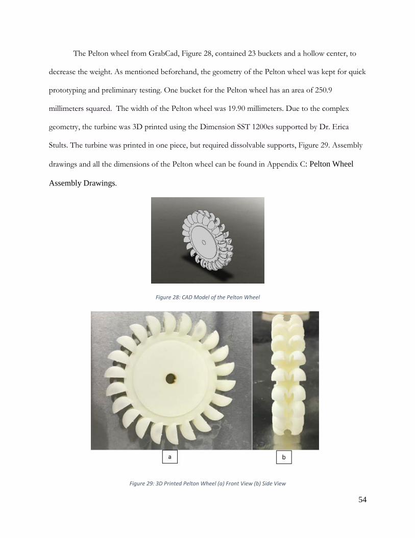
54

The Pelton wheel from GrabCad, Figure 28, contained 23 buckets and a hollow center, to

decrease the weight. As mentioned beforehand, the geometry of the Pelton wheel was kept for quick

prototyping and preliminary testing. One bucket for the Pelton wheel has an area of 250.9

millimeters squared. The width of the Pelton wheel was 19.90 millimeters. Due to the complex

geometry, the turbine was 3D printed using the Dimension SST 1200es supported by Dr. Erica

Stults. The turbine was printed in one piece, but required dissolvable supports, Figure 29. Assembly

drawings and all the dimensions of the Pelton wheel can be found in Appendix C: Pelton Wheel

Assembly Drawings.

Figure 28: CAD Model of the Pelton Wheel

Figure 29: 3D Printed Pelton Wheel (a) Front View (b) Side View

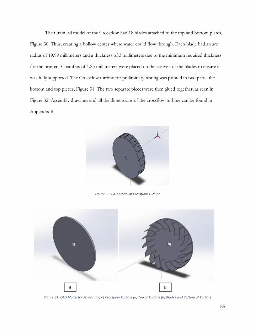
55

The GrabCad model of the Crossflow had 18 blades attached to the top and bottom plates,

Figure 30. Thus, creating a hollow center where water could flow through. Each blade had an arc

radius of 19.99 millimeters and a thickness of 3 millimeters due to the minimum required thickness

for the printer. Chamfers of 1.85 millimeters were placed on the convex of the blades to ensure it

was fully supported. The Crossflow turbine for preliminary testing was printed in two parts, the

bottom and top pieces, Figure 31. The two separate pieces were then glued together, as seen in

Figure 32. Assembly drawings and all the dimensions of the crossflow turbine can be found in

Appendix B.

Figure 30: CAD Model of Crossflow Turbine

Figure 31: CAD Model for 3D Printing of Crossflow Turbine (a) Top of Turbine (b) Blades and Bottom of Turbine

56

Figure 32: 3D Printed Crossflow Turbine (a) Top View (b) Side View

SolidWorks Simulations

In order to evaluate the turbines, static stress, displacement, and strain simulations were

analyzed using SolidWorks. These analyses were used to determine the amount of stress,

displacement, and strain the turbines could withstand in the system. All simulations were run with

ABS material to replicate our 3D printing, which has a yield strength of 40 MPa. Pressure was used

as the normal load on the areas of impact, which differed for each turbine. The area of impact was

determined using preliminary water testing and marking the location for different GPM. The static

analysis did not include atmospheric pressure; thus the pressure was added to the final calculations.

The pressure was calculated by Equation 30:

𝑃𝑃 = 𝜌𝜌 ∗ 𝑔𝑔 ∗ ℎ (30)

Where:

𝑃𝑃 = 𝑃𝑃𝐹𝐹𝐻𝐻𝐿𝐿𝐿𝐿𝑢𝑢𝐹𝐹𝐻𝐻 (𝑃𝑃𝐻𝐻)

𝜌𝜌 = 𝐷𝐷𝐻𝐻𝐹𝐹𝐿𝐿𝐹𝐹𝐹𝐹𝑉𝑉 𝐿𝐿𝑓𝑓 𝑊𝑊𝐻𝐻𝐹𝐹𝐻𝐻𝐹𝐹 𝐻𝐻𝐹𝐹 20 𝐶𝐶𝐻𝐻𝑢𝑢𝐹𝐹𝐹𝐹𝑢𝑢𝐿𝐿 �𝑘𝑘𝑔𝑔𝑚𝑚3�

57

𝑔𝑔 = 𝐺𝐺𝐹𝐹𝐻𝐻𝐺𝐺𝐹𝐹𝐹𝐹𝑉𝑉 �𝑚𝑚𝐿𝐿2 �

ℎ = 𝐻𝐻𝐻𝐻𝐹𝐹𝑔𝑔ℎ𝐹𝐹 (𝑚𝑚)

𝑃𝑃 = 998.2067 ∗ 9.98 ∗ 4

𝑃𝑃 = 3.98 ∗ 104 𝑃𝑃𝐻𝐻 = 5.78 𝑃𝑃𝐿𝐿𝐹𝐹

5.78 𝑃𝑃𝐿𝐿𝐹𝐹 + 14.7 𝑃𝑃𝐿𝐿𝐹𝐹 (𝐻𝐻𝐹𝐹𝑚𝑚𝐿𝐿𝐿𝐿𝑃𝑃ℎ𝐻𝐻𝐹𝐹𝐹𝐹𝐹𝐹 𝑃𝑃𝐹𝐹𝐻𝐻𝐿𝐿𝐿𝐿𝑢𝑢𝐹𝐹𝐻𝐻) = 20.78 𝑃𝑃𝐿𝐿𝐹𝐹

For each of the simulations, connections, fixtures, external loads, and a mesh were created

and defined. The component contacts for the turbines were defined as bonded and the turbines

were fixed at the key shaft. The pressure was set to 20.48 Psi on certain points on each turbine. The

pressure points were determined from preliminary water testing done on the printed models and will

be shown in this section. A shear mesh was created on the entire model. Figure 33, shows the steps

to run the simulation.

Figure 33: Steps for SolidWorks Simulation

In order to evaluate the strain on each of the turbines, a stress-strain graph was analyzed to

ensure that the impact of the normal force did not cause the material to pass its yield strength,

Figure 34.

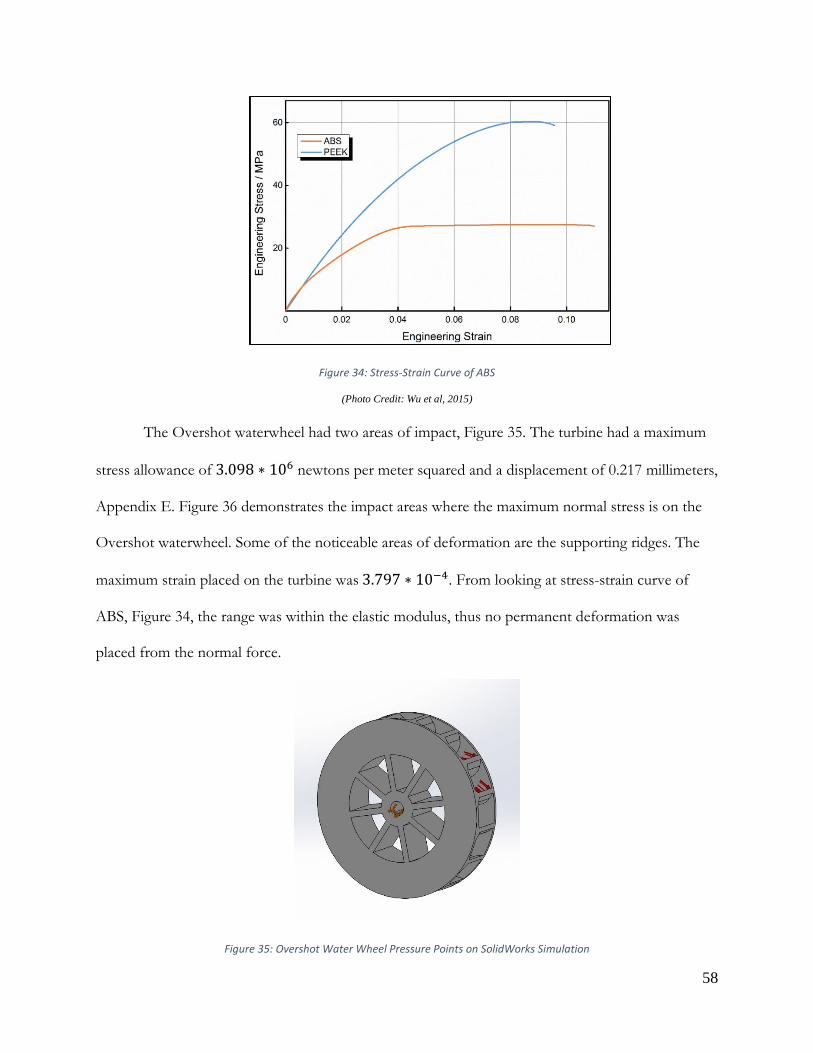
58

Figure 34: Stress-Strain Curve of ABS

(Photo Credit: Wu et al, 2015)

The Overshot waterwheel had two areas of impact, Figure 35. The turbine had a maximum

stress allowance of 3.098 ∗ 106 newtons per meter squared and a displacement of 0.217 millimeters,

Appendix E. Figure 36 demonstrates the impact areas where the maximum normal stress is on the

Overshot waterwheel. Some of the noticeable areas of deformation are the supporting ridges. The

maximum strain placed on the turbine was 3.797 ∗ 10−4. From looking at stress-strain curve of

ABS, Figure 34, the range was within the elastic modulus, thus no permanent deformation was

placed from the normal force.

Figure 35: Overshot Water Wheel Pressure Points on SolidWorks Simulation

59

Figure 36: Overshot Water Wheel Static Stress SolidWorks Simulation Results

From preliminary testing, it was determined that the areas of impact were two buckets on

the Pelton wheel, Figure 37. The Pelton had the largest stress threshold with 1.406 ∗ 107Pascals, as

shown on Figure 38. The displacement for the wheel was 0.073 millimeters, Appendix F. With a

strain of 3.357 ∗ 10−4 for the 3D printed ABS plastic, the stress-strain fell in the elastic modulus

range, Figure 34, thus no permanent deformation on the material.

Figure 37: Pelton Wheel Pressure Points on SolidWorks Simulation

60

Figure 38: Pelton Wheel Static Stress SolidWorks Simulation

Lastly, the Crossflow turbine had two blades in the area of impact, Figure 39. The

simulations determined that the turbine could withstand normal stress up to 3.642 ∗ 106 Pascals.

In addition, displacement of the blades could range from 1.0 * 10-30 millimeters to 0.1383 millimeters

under the given pressure, Appendix G. Most of the deformation in the model was seen in the

connection of the blades to the top and bottom plates, Figure 40. The normal strain of the ABS

plastic was 5.545 ∗ 10−4. From looking at Figure 34, we can determine that the stress-strain in the

range of the elastic modulus and causing no permanent deformation.

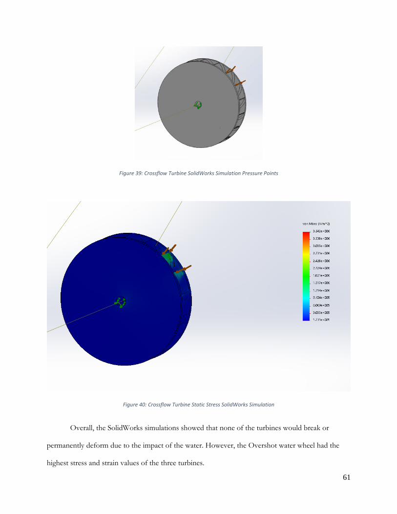
61

Figure 39: Crossflow Turbine SolidWorks Simulation Pressure Points

Figure 40: Crossflow Turbine Static Stress SolidWorks Simulation

Overall, the SolidWorks simulations showed that none of the turbines would break or

permanently deform due to the impact of the water. However, the Overshot water wheel had the

highest stress and strain values of the three turbines.

62

Preliminary Stall Torque and RPM Testing The 10-centimeter diameter Overshot water wheel, Pelton, and Crossflow were put through

preliminary stall torque and RPM tests, in order to support findings from the SolidWorks analysis.

The tests were performed by placing the turbines into the turbine casing and using torque and RPM

readers. To measure the RPMs, a digital tachometer made by Neiko was used. The tachometer can

read up to 99,999 RPM with an accuracy of +/- 0.05 percent. The analog torque meter, made by

Waters, had a range of 0 to 40 ounce-inches and is accurate to the ones place. All tests were

accomplished with an approximate flow rate of 8 GPM held 1 meter above the turbine. Three trials

of 50 data points each were taken and used to calculate the standard deviation and average for each

RPM trial for each turbine. Similarly, three trials of stall torque data were taken for each turbine and

calculated to have the average and standard deviation. The results are summarized in Table 5 below.

Table 5: Results of 10 cm Turbine Testing at 8 GPM

Pelton Crossflow Overshot

Speed (RPM) 679 ± 32.0 652 ± 85.2 646 ± 55.0

Stall Torque (oz-in)

12 ± 0.0 18 ± 0.06 5 ± 0.6

The overall data presented that the Overshot water wheel had the lowest torque and RPM

values. The Pelton wheel and Crossflow turbines had the greatest potential for power output based

on the RPM and torque values. Due to the results of the testing and the SolidWorks simulations, the

Overshot water wheel was eliminated.

63

Design and Optimization of Pelton and Crossflow

After the elimination of the Overshot water wheel, the Pelton and Crossflow were

optimized, resized, reprinted, and tested in order to select the final turbine. Previously, the turbines

had been sized and printed at an outer diameter of 10 centimeters to save material and fit on the

printer beds. Due to the low stall torques found in preliminary testing, the turbines were resized to

20 centimeters and the number of blades was optimized at the 20 centimeter diameter size to

improve performance.

The first step in redesigning the turbines was to optimize them for the system. Particularly,

the Pelton’s optimization depended on the jet diameter of our downspout, the size range of the

turbine (pico, micro, etc.), and the wheel diameter. The downspout jet diameter for the testing was 1

inch. The Equation 31 was used to determine the ideal number of buckets:

𝑁𝑁𝑏𝑏 = 𝐷𝐷𝑝𝑝𝐻𝐻𝑗𝑗

+ 15 (31)

(Zidonis et al, 2014, pg. 2)

Where:

𝑁𝑁𝑏𝑏 = 𝐼𝐼𝐻𝐻𝐻𝐻𝐻𝐻𝑢𝑢 𝑁𝑁𝑢𝑢𝑚𝑚𝑁𝑁𝐻𝐻𝐹𝐹 𝐿𝐿𝑓𝑓 𝐵𝐵𝑢𝑢𝐹𝐹𝑘𝑘𝐻𝐻𝐹𝐹𝐿𝐿 (𝑢𝑢𝐹𝐹𝐹𝐹𝐹𝐹𝑢𝑢𝐻𝐻𝐿𝐿𝐿𝐿)

𝐷𝐷𝑃𝑃 = 𝑊𝑊ℎ𝐻𝐻𝐻𝐻𝑢𝑢 𝐷𝐷𝐹𝐹𝐻𝐻𝑚𝑚𝐻𝐻𝐹𝐹𝐻𝐻𝐹𝐹 (𝐹𝐹𝐹𝐹𝐹𝐹ℎ𝐻𝐻𝐿𝐿)

𝐻𝐻𝑗𝑗 = 𝐽𝐽𝐻𝐻𝐹𝐹 𝐷𝐷𝐹𝐹𝐻𝐻𝑚𝑚𝐻𝐻𝐹𝐹𝐻𝐻𝐹𝐹 (𝐹𝐹𝐹𝐹𝐹𝐹ℎ𝐻𝐻𝐿𝐿)

For 20 centimeter Pelton wheel:

20 𝐹𝐹𝑚𝑚 = 7.9 𝐹𝐹𝐹𝐹𝐹𝐹ℎ𝐻𝐻𝐿𝐿

𝑁𝑁𝑏𝑏 = 7.91

+ 15

64

𝑁𝑁𝑏𝑏 = 23 𝑁𝑁𝑢𝑢𝐹𝐹𝑘𝑘𝐻𝐻𝐹𝐹𝐿𝐿

In order to optimize the Crossflow turbine, the number of runner blades, blade spacing and

the inlet angle of the blades need to be evaluated for the size and outer diameter. It has been

determined that the optimized blade inlet angle is 30 degrees (Win et al, 2008).

Equation 32 and Equation 33 were used to evaluate the number of runner blades:

𝐹𝐹 = 𝜋𝜋 ∗ 𝐷𝐷1𝐹𝐹

(32)

𝐹𝐹 = 𝑘𝑘 ∗ 𝐷𝐷1𝐿𝐿𝐹𝐹𝐹𝐹𝑐𝑐1

(33)

(Win et al, 2016)

Where:

𝐹𝐹 = 𝐼𝐼𝐻𝐻𝐻𝐻𝐻𝐻𝑢𝑢 𝑁𝑁𝑢𝑢𝑚𝑚𝑁𝑁𝐻𝐻𝐹𝐹 𝐿𝐿𝑓𝑓 𝑁𝑁𝑢𝑢𝐹𝐹𝑘𝑘𝐻𝐻𝐹𝐹𝐿𝐿 (𝑢𝑢𝐹𝐹𝐹𝐹𝐹𝐹𝑢𝑢𝐻𝐻𝐿𝐿𝐿𝐿)

𝐷𝐷1 = 𝑂𝑂𝑢𝑢𝐹𝐹𝐻𝐻𝐹𝐹 𝐷𝐷𝐹𝐹𝐻𝐻𝑚𝑚𝐻𝐻𝐹𝐹𝐻𝐻𝐹𝐹 (𝐹𝐹𝑚𝑚)

𝐹𝐹 = 𝐵𝐵𝑢𝑢𝐻𝐻𝐻𝐻𝐻𝐻 𝑆𝑆𝑃𝑃𝐻𝐻𝐹𝐹𝐹𝐹𝐹𝐹𝑔𝑔 (𝐹𝐹𝑚𝑚)

𝑘𝑘 = 0.075

For 20 centimeter Crossflow turbine:

𝐹𝐹 = 0.075 ∗ 20

sin (30)= 3

𝐹𝐹 = 𝜋𝜋 ∗ 20

3= 21 𝑁𝑁𝑢𝑢𝐻𝐻𝐻𝐻𝐻𝐻𝐿𝐿

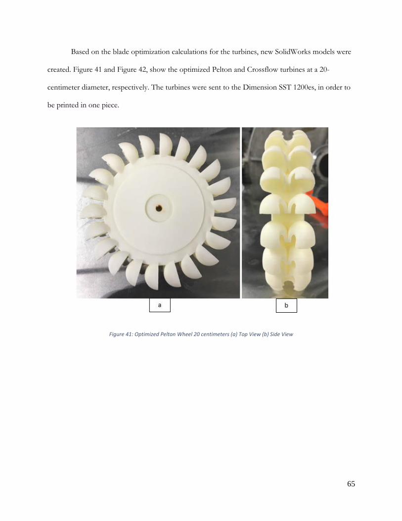
65

Based on the blade optimization calculations for the turbines, new SolidWorks models were

created. Figure 41 and Figure 42, show the optimized Pelton and Crossflow turbines at a 20-

centimeter diameter, respectively. The turbines were sent to the Dimension SST 1200es, in order to

be printed in one piece.

Figure 41: Optimized Pelton Wheel 20 centimeters (a) Top View (b) Side View

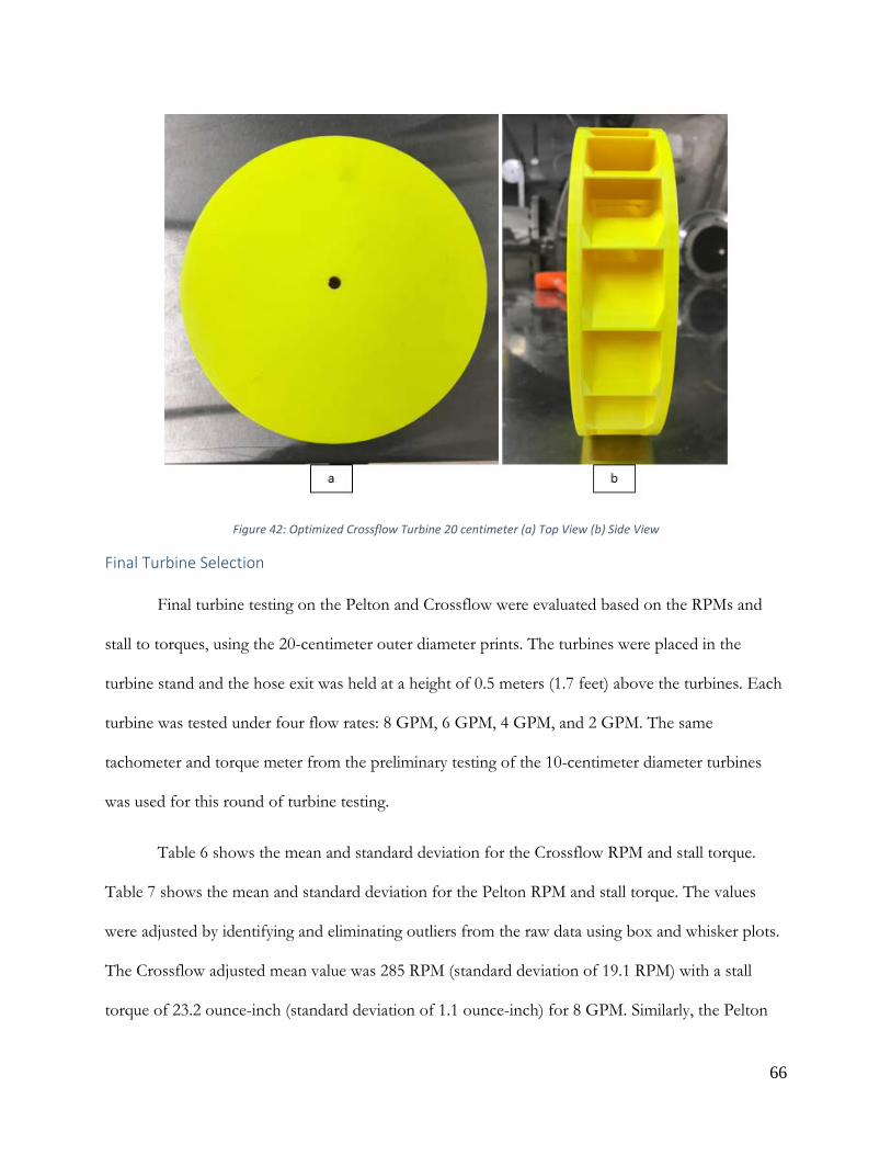
66

Figure 42: Optimized Crossflow Turbine 20 centimeter (a) Top View (b) Side View

Final Turbine Selection

Final turbine testing on the Pelton and Crossflow were evaluated based on the RPMs and

stall to torques, using the 20-centimeter outer diameter prints. The turbines were placed in the

turbine stand and the hose exit was held at a height of 0.5 meters (1.7 feet) above the turbines. Each

turbine was tested under four flow rates: 8 GPM, 6 GPM, 4 GPM, and 2 GPM. The same

tachometer and torque meter from the preliminary testing of the 10-centimeter diameter turbines

was used for this round of turbine testing.

Table 6 shows the mean and standard deviation for the Crossflow RPM and stall torque.

Table 7 shows the mean and standard deviation for the Pelton RPM and stall torque. The values

were adjusted by identifying and eliminating outliers from the raw data using box and whisker plots.

The Crossflow adjusted mean value was 285 RPM (standard deviation of 19.1 RPM) with a stall

torque of 23.2 ounce-inch (standard deviation of 1.1 ounce-inch) for 8 GPM. Similarly, the Pelton

67

had a mean of 328 RPM (standard deviation of 7.70 RPM), and a stall torque of 24 ounce-inch

(standard deviation of 2.5 ounce-inch). Because the turbine values were very similar to each other

during the tests, the final selection was determined using the data gathered from power outcome

during the entire system testing, found in the 4.0 Testing Section.

Table 6: Results of Preliminary Crossflow Testing

Flow rate (GPM) 8 6 4 2

Mean Rotational Speed (RPM) 285±19.1 260±7.1 192±17.1 188±18.9

Mean Stall Torque (oz.-in.) 23.2±1.1 9±0.58 6±0.6 3±0.6

Table 7: Results of Preliminary Pelton Testing


Mean Rotational Speed (RPM) 328±7.70 272±11.3 207±11.9 212±11.8

Mean Stall Torque (oz.-in.) 24±2.5 13±0.58 11±0.0 7±0.6

In order to put the RPM and torque values for both of the turbines into perspective, the

theoretical power was calculated. The theoretical maximum power can be derived by using Equation

34, Equation 35, and Equation 36. In Equation 34, the relationship between torque and angular

velocity is presented as linear with a slope of k. The proof for this relationship is in Section 4.1 and

is directly shown in Equation 54.

𝑇𝑇 = 𝑇𝑇𝑚𝑚𝐶𝐶𝑥𝑥 + 𝑘𝑘 ∗ 𝐹𝐹 (34)

𝑘𝑘 = −𝑇𝑇𝑚𝑚𝐶𝐶𝑥𝑥𝐹𝐹𝑚𝑚𝐶𝐶𝑥𝑥

(35)

𝑃𝑃 = 𝑇𝑇 ∗ 𝐹𝐹 (36)

68

Where:

𝑃𝑃 = 𝑃𝑃𝐿𝐿𝐹𝐹𝐻𝐻𝐹𝐹 (𝑊𝑊𝐻𝐻𝐹𝐹𝐹𝐹𝐿𝐿)

𝑇𝑇 = 𝑇𝑇𝐿𝐿𝐹𝐹𝑠𝑠𝑢𝑢𝐻𝐻 (𝑁𝑁𝑚𝑚)

𝑇𝑇𝑚𝑚𝐶𝐶𝑥𝑥 = 𝑀𝑀𝐻𝐻𝐸𝐸𝐹𝐹𝑚𝑚𝑢𝑢𝑚𝑚 𝑇𝑇𝐿𝐿𝐹𝐹𝑠𝑠𝑢𝑢𝐻𝐻 , 𝑆𝑆𝐹𝐹𝐻𝐻𝑢𝑢𝑢𝑢 𝑇𝑇𝐿𝐿𝐹𝐹𝑠𝑠𝑢𝑢𝐻𝐻 (𝑁𝑁𝑚𝑚)

𝐹𝐹 = 𝐴𝐴𝐹𝐹𝑔𝑔𝑢𝑢𝑢𝑢𝐻𝐻𝐹𝐹 𝑉𝑉𝐻𝐻𝑢𝑢𝐿𝐿𝐹𝐹𝐹𝐹𝐹𝐹𝑉𝑉 𝐿𝐿𝑓𝑓 𝑇𝑇𝑢𝑢𝐹𝐹𝑁𝑁𝐹𝐹𝐹𝐹𝐻𝐻 (𝐹𝐹𝐻𝐻𝐻𝐻/𝐿𝐿)

𝐹𝐹𝑚𝑚𝐶𝐶𝑥𝑥 = 𝑀𝑀𝐻𝐻𝐸𝐸𝐹𝐹𝑚𝑚𝑢𝑢𝑚𝑚 𝐴𝐴𝐹𝐹𝑔𝑔𝑢𝑢𝑢𝑢𝐻𝐻𝐹𝐹 𝑉𝑉𝐻𝐻𝑢𝑢𝐿𝐿𝐹𝐹𝐹𝐹𝐹𝐹𝑉𝑉, 𝐹𝐹. 𝐻𝐻.𝐹𝐹𝐹𝐹𝐻𝐻𝐻𝐻𝐹𝐹ℎ𝐻𝐻𝐻𝐻𝑢𝑢 (𝐹𝐹𝐻𝐻𝐻𝐻/𝐿𝐿)

𝑘𝑘 = 𝑆𝑆𝑢𝑢𝐿𝐿𝑃𝑃𝐻𝐻 (𝑇𝑇/𝐹𝐹)

Using these equations, the angular velocity can be seen in Equation 38 and the torque at the

maximum power can be seen in Equation 39:

𝑃𝑃 = (𝑇𝑇𝑚𝑚𝐶𝐶𝑥𝑥 + 𝑘𝑘 ∗ 𝐹𝐹) ∗ 𝐹𝐹

𝑃𝑃 = 𝑇𝑇𝑚𝑚𝐶𝐶𝑥𝑥 ∗ 𝐹𝐹 + 𝑘𝑘 ∗ 𝐹𝐹2

𝐻𝐻𝑃𝑃𝐻𝐻𝐹𝐹

= 𝑇𝑇𝑚𝑚𝐶𝐶𝑥𝑥 + 2 ∗ 𝑘𝑘 ∗ 𝐹𝐹

To maximize power:

0 = 𝑇𝑇𝑚𝑚𝐶𝐶𝑥𝑥 + 2 ∗ 𝑘𝑘 ∗ 𝐹𝐹

Solving for angular velocity:

𝐹𝐹 =−𝑇𝑇𝑚𝑚𝐶𝐶𝑥𝑥2 ∗ 𝑘𝑘

𝐹𝐹 =−𝑇𝑇𝑚𝑚𝐶𝐶𝑥𝑥

2 �−𝑇𝑇𝑚𝑚𝐶𝐶𝑥𝑥𝐹𝐹𝑚𝑚𝐶𝐶𝑥𝑥�

𝐹𝐹 =𝐹𝐹𝑚𝑚𝐶𝐶𝑥𝑥

2 (38)

Knowing the angular velocity at maximum power the torque at maximum power can be

determined:

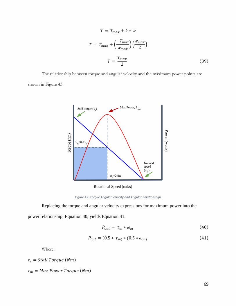
69

𝑇𝑇 = 𝑇𝑇𝑚𝑚𝐶𝐶𝑥𝑥 + 𝑘𝑘 ∗ 𝐹𝐹

𝑇𝑇 = 𝑇𝑇𝑚𝑚𝐶𝐶𝑥𝑥 + �−𝑇𝑇𝑚𝑚𝐶𝐶𝑥𝑥𝐹𝐹𝑚𝑚𝐶𝐶𝑥𝑥

� �𝐹𝐹𝑚𝑚𝐶𝐶𝑥𝑥

2�

𝑇𝑇 = 𝑇𝑇𝑚𝑚𝐶𝐶𝑥𝑥

2 (39)

The relationship between torque and angular velocity and the maximum power points are

shown in Figure 43.

Figure 43: Torque Angular Velocity and Angular Relationships

Replacing the torque and angular velocity expressions for maximum power into the

power relationship, Equation 40, yields Equation 41:

𝑃𝑃𝐶𝐶𝐶𝐶𝐶𝐶 = 𝜏𝜏𝑚𝑚 ∗ 𝜔𝜔𝑚𝑚 (40)

𝑃𝑃𝐶𝐶𝐶𝐶𝐶𝐶 = (0.5 ∗ 𝜏𝜏𝑚𝑚) ∗ (0.5 ∗ 𝜔𝜔𝑚𝑚) (41)

Where:

𝜏𝜏𝑠𝑠 = 𝑆𝑆𝐹𝐹𝐻𝐻𝑢𝑢𝑢𝑢 𝑇𝑇𝐿𝐿𝐹𝐹𝑠𝑠𝑢𝑢𝐻𝐻 (𝑁𝑁𝑚𝑚)

𝜏𝜏𝑚𝑚 = 𝑀𝑀𝐻𝐻𝐸𝐸 𝑃𝑃𝐿𝐿𝐹𝐹𝐻𝐻𝐹𝐹 𝑇𝑇𝐿𝐿𝐹𝐹𝑠𝑠𝑢𝑢𝐻𝐻 (𝑁𝑁𝑚𝑚)

70

𝜔𝜔𝐶𝐶 = 𝐹𝐹𝐹𝐹𝐻𝐻𝐻𝐻 𝑊𝑊ℎ𝐻𝐻𝐻𝐻𝑢𝑢 𝐴𝐴𝐹𝐹𝑔𝑔𝑢𝑢𝑢𝑢𝐻𝐻𝐹𝐹 𝑆𝑆𝑃𝑃𝐻𝐻𝐻𝐻𝐻𝐻 �𝐹𝐹𝐻𝐻𝐻𝐻𝐿𝐿�

𝜔𝜔𝑚𝑚 = 𝑀𝑀𝐻𝐻𝐸𝐸 𝑃𝑃𝐿𝐿𝐹𝐹𝐻𝐻𝐹𝐹 𝐴𝐴𝐹𝐹𝑔𝑔𝑢𝑢𝑢𝑢𝐻𝐻𝐹𝐹 𝑆𝑆𝑃𝑃𝐻𝐻𝐻𝐻𝐻𝐻 �𝐹𝐹𝐻𝐻𝐻𝐻𝐿𝐿�

To convert the measured torque from ounce-inches to Newton-meters, and the measured

angular velocity from RPMs to radians per second, Equations 42 and 43 were used respectively:

𝜏𝜏𝑁𝑁∙𝑚𝑚 = 𝜏𝜏𝐶𝐶𝑜𝑜∙𝐶𝐶𝐶𝐶 ∗ �1 𝑁𝑁 ∙ 𝑚𝑚

141.6 𝐿𝐿𝑜𝑜 ∙ 𝐹𝐹𝐹𝐹� (42)

𝜔𝜔𝐶𝐶𝐶𝐶𝑟𝑟𝑠𝑠

= 𝜔𝜔𝑅𝑅𝑃𝑃𝑅𝑅 ∗ �2𝜋𝜋 𝐹𝐹𝐻𝐻𝐻𝐻

𝐹𝐹𝐻𝐻𝐺𝐺𝐿𝐿𝑢𝑢𝑢𝑢𝐹𝐹𝐹𝐹𝐿𝐿𝐹𝐹� ∗ �

1 𝑚𝑚𝐹𝐹𝐹𝐹𝑢𝑢𝐹𝐹𝐻𝐻60 𝐿𝐿𝐻𝐻𝐹𝐹𝐿𝐿𝐹𝐹𝐻𝐻𝐿𝐿

� (43)

Figure 44 displays the theoretical power calculations for the Pelton and Crossflow using the

RPM and stall torque data and the equations described above.

Figure 44: Maximum Power Calculations Pelton vs Crossflow

71

The line of best fit in Figure 44 shows a cubic relationship between the power output and

the flow. The cubic relationship that we observed aligns with theory because in this experimental

setup the water was directed onto the turbine by a hose held at 0.5 meters (1.7 feet) above the

turbine. In this case, the kinetic energy is not negligible because it is about equal in magnitude to the

potential energy. The cubic relationship can be derived observed in the following Power analysis,

Equation 44:

𝑃𝑃 = 12∗ 𝑚𝑚 ∗ 𝐺𝐺2 + 𝑚𝑚 ∗ 𝑔𝑔 ∗ ℎ (44)

𝑃𝑃 = 12∗ [ 𝑄𝑄 ∗ 𝜌𝜌] ∗ �

𝑄𝑄𝐴𝐴�2

+ 𝑄𝑄 ∗ 𝜌𝜌 ∗ 𝑔𝑔 ∗ ℎ

Where:


𝑚𝑚 = 𝑀𝑀𝐻𝐻𝐿𝐿𝐿𝐿 𝐹𝐹𝑢𝑢𝐿𝐿𝐹𝐹 𝑅𝑅𝐻𝐻𝐹𝐹𝐻𝐻 𝐿𝐿𝑓𝑓 𝑊𝑊𝐻𝐻𝐹𝐹𝐻𝐻𝐹𝐹 �𝑘𝑘𝑔𝑔𝐿𝐿�

𝐺𝐺 = 𝑉𝑉𝐻𝐻𝑢𝑢𝐿𝐿𝐹𝐹𝐹𝐹𝐹𝐹𝑉𝑉 𝐿𝐿𝑓𝑓 𝑊𝑊𝐻𝐻𝐹𝐹𝐻𝐻𝐹𝐹 𝑓𝑓𝐹𝐹𝐿𝐿𝑚𝑚 𝐹𝐹ℎ𝐻𝐻 𝐻𝐻𝐿𝐿𝐿𝐿𝐻𝐻 �𝑚𝑚𝐿𝐿�

𝑄𝑄 = 𝑉𝑉𝐿𝐿𝑢𝑢𝑢𝑢𝑚𝑚𝐻𝐻𝐹𝐹𝐹𝐹𝐹𝐹𝐹𝐹 𝐹𝐹𝑢𝑢𝐿𝐿𝐹𝐹 𝑅𝑅𝐻𝐻𝐹𝐹𝐻𝐻 �𝑚𝑚3

𝐿𝐿�


𝐴𝐴 = 𝐶𝐶𝐹𝐹𝐿𝐿𝐿𝐿𝐿𝐿 𝑆𝑆𝐻𝐻𝐹𝐹𝐹𝐹𝐹𝐹𝐿𝐿𝐹𝐹𝐻𝐻𝑢𝑢 𝐴𝐴𝐹𝐹𝐻𝐻𝐻𝐻 𝐿𝐿𝑓𝑓 𝐻𝐻𝐿𝐿𝐿𝐿𝐻𝐻 (𝑚𝑚2)

𝑔𝑔 = 𝐺𝐺𝐹𝐹𝐻𝐻𝐺𝐺𝐹𝐹𝐹𝐹𝐻𝐻𝐹𝐹𝐹𝐹𝐿𝐿𝐹𝐹𝐻𝐻𝑢𝑢 𝐴𝐴𝐹𝐹𝐹𝐹𝐻𝐻𝑢𝑢𝐻𝐻𝐹𝐹𝐻𝐻𝐹𝐹𝐹𝐹𝐿𝐿𝐹𝐹 �𝑚𝑚𝐿𝐿2�

ℎ = 𝐻𝐻𝐻𝐻𝐹𝐹𝑔𝑔ℎ𝐹𝐹 (𝑚𝑚)

This brief theoretical check proves that a cubic relationship between flow and power, plus an

offset that is related to the flow and height, exists at a low height exists.

72

3.6 Electrical Component Selection

Direct current permanent magnet motors were researched with RPM and torque ranges that

were compatible with the output from our turbines, maximum RPMs in the range of 300 to 500 and

maximum torques from 10 to 20 ounce-inches. Through the research, we found a micro gear motor

rated at a max speed of 460 RPM and a stall torque of 20-ounce inch sold by Sparkfun. Once the

motor was purchased, the internal resistance of the motor was measured using a multimeter and was

found to be 16.7 Ohms. This resistance was cross checked by measuring the open circuit voltage of

the motor and then adding a resistance of 16.5 Ohms externally and re-measuring the voltage. The

open circuit voltage was 6 volts and the voltage drop in the second setup with the voltage divider

resistor had a voltage of 3 volts. This proved that the motor’s internal resistance was about 16.7

Ohms. Additionally, the 16.5 Ohm resistance was utilized to model a load. It was chosen because

the maximum power delivered to a load is when the resistance externally matches the Thevenin

equivalent resistance of the power source, this is derived in Jacobi’s Law.

To actually generate power, the motor output shaft was connected to the turbine stand and

shaft and the wire leads were connected to a circuit. With this configuration the motor became a

generator. The generator’s max speed and stall torque were compared to the experimentally

measured stall torque and RPM outputs to confirm its compatibility. The generator’s 3 millimeter

shaft was rated for a torque of 20 ounce inch and speed was rated for 460 RPM. The turbine shaft

and generator shaft were connected as done through a series of two spur gears shown in Figure 45.

Figure 45: Series of Two Spur Gears

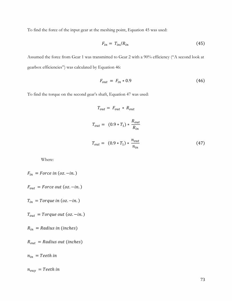
73

To find the force of the input gear at the meshing point, Equation 45 was used:

𝐹𝐹𝐶𝐶𝐶𝐶 = 𝑇𝑇𝐶𝐶𝐶𝐶/𝑅𝑅𝐶𝐶𝐶𝐶 (45)

Assumed the force from Gear 1 was transmitted to Gear 2 with a 90% efficiency (“A second look at

gearbox efficiencies”) was calculated by Equation 46:

𝐹𝐹𝐶𝐶𝐶𝐶𝐶𝐶 = 𝐹𝐹𝐶𝐶𝐶𝐶 ∗ 0.9 (46)

To find the torque on the second gear’s shaft, Equation 47 was used:

𝑇𝑇𝐶𝐶𝐶𝐶𝐶𝐶 = 𝐹𝐹𝐶𝐶𝐶𝐶𝐶𝐶 ∗ 𝑅𝑅𝐶𝐶𝐶𝐶𝐶𝐶

𝑇𝑇𝐶𝐶𝐶𝐶𝐶𝐶 = (0.9 ∗ 𝑇𝑇1) ∗ 𝑅𝑅𝐶𝐶𝐶𝐶𝐶𝐶𝑅𝑅𝐶𝐶𝐶𝐶

𝑇𝑇𝐶𝐶𝐶𝐶𝐶𝐶 = (0.9 ∗ 𝑇𝑇1) ∗ 𝐹𝐹𝐶𝐶𝐶𝐶𝐶𝐶𝐹𝐹𝐶𝐶𝐶𝐶

(47)

Where:

𝐹𝐹𝐶𝐶𝐶𝐶 = 𝐹𝐹𝐿𝐿𝐹𝐹𝐹𝐹𝐻𝐻 𝐹𝐹𝐹𝐹 (𝐿𝐿𝑜𝑜.−𝐹𝐹𝐹𝐹. )

𝐹𝐹𝐶𝐶𝐶𝐶𝐶𝐶 = 𝐹𝐹𝐿𝐿𝐹𝐹𝐹𝐹𝐻𝐻 𝐿𝐿𝑢𝑢𝐹𝐹 (𝐿𝐿𝑜𝑜.−𝐹𝐹𝐹𝐹. )

𝑇𝑇𝐶𝐶𝐶𝐶 = 𝑇𝑇𝐿𝐿𝐹𝐹𝑠𝑠𝑢𝑢𝐻𝐻 𝐹𝐹𝐹𝐹 (𝐿𝐿𝑜𝑜.−𝐹𝐹𝐹𝐹. )

𝑇𝑇𝐶𝐶𝐶𝐶𝐶𝐶 = 𝑇𝑇𝐿𝐿𝐹𝐹𝑠𝑠𝑢𝑢𝐻𝐻 𝐿𝐿𝑢𝑢𝐹𝐹 (𝐿𝐿𝑜𝑜.−𝐹𝐹𝐹𝐹. )

𝑅𝑅𝐶𝐶𝐶𝐶 = 𝑅𝑅𝐻𝐻𝐻𝐻𝐹𝐹𝑢𝑢𝐿𝐿 𝐹𝐹𝐹𝐹 (𝐹𝐹𝐹𝐹𝐹𝐹ℎ𝐻𝐻𝐿𝐿)

𝑅𝑅𝐶𝐶𝐶𝐶𝐶𝐶 = 𝑅𝑅𝐻𝐻𝐻𝐻𝐹𝐹𝑢𝑢𝐿𝐿 𝐿𝐿𝑢𝑢𝐹𝐹 (𝐹𝐹𝐹𝐹𝐹𝐹ℎ𝐻𝐻𝐿𝐿)

𝐹𝐹𝐶𝐶𝐶𝐶 = 𝑇𝑇𝐻𝐻𝐻𝐻𝐹𝐹ℎ 𝐹𝐹𝐹𝐹

𝐹𝐹𝐶𝐶𝐶𝐶𝑦𝑦 = 𝑇𝑇𝐻𝐻𝐻𝐻𝐹𝐹ℎ 𝐹𝐹𝐹𝐹

74

The torque output was solved for the maximum output stall torque:

𝑇𝑇𝐶𝐶𝐶𝐶𝐶𝐶 = 0.9 ∗ 26.5 ∗2430

𝑇𝑇𝐶𝐶𝐶𝐶𝐶𝐶 = 19.08 𝐿𝐿𝑜𝑜.−𝐹𝐹𝐹𝐹.

This output torque was determined using the highest 𝑇𝑇𝐶𝐶𝐶𝐶 value that we experienced during

testing. The 𝑇𝑇𝐶𝐶𝐶𝐶𝐶𝐶 value falls within the 20 ounce-inch threshold of the motor.

Next we compared the RPM rating of the motor to the max RPM output from the turbine

using Equation 48.

𝑊𝑊𝐶𝐶𝐶𝐶𝐶𝐶 = 𝑁𝑁𝐶𝐶𝐶𝐶𝑁𝑁𝐶𝐶𝐶𝐶𝐶𝐶

∗ 𝑊𝑊𝐶𝐶𝐶𝐶 (48)

Where:

𝑊𝑊𝐶𝐶𝐶𝐶𝐶𝐶 = 𝑅𝑅𝑃𝑃𝑀𝑀 𝐿𝐿𝑢𝑢𝐹𝐹

𝑊𝑊𝐶𝐶𝐶𝐶 = 𝑅𝑅𝑃𝑃𝑀𝑀 𝐹𝐹𝐹𝐹

𝑁𝑁𝐶𝐶𝐶𝐶𝐶𝐶 = 𝑇𝑇𝐻𝐻𝐻𝐻𝐹𝐹ℎ 𝐿𝐿𝑢𝑢𝐹𝐹

𝑁𝑁𝐶𝐶𝐶𝐶 = 𝑇𝑇𝐻𝐻𝐻𝐻𝐹𝐹ℎ 𝐹𝐹𝐹𝐹

𝑊𝑊𝐶𝐶𝐶𝐶𝐶𝐶 = 3024

∗ 470

𝑊𝑊𝐶𝐶𝐶𝐶𝐶𝐶 = 587.5 𝑅𝑅𝑃𝑃𝑀𝑀

The maximum RPM of the motor shaft is 587.5 RPM which is above the 460 RPM

threshold of the motor. Because this RPM is the freewheel RPM of the turbine, this value should

75

not be reached. Therefore, after analyzing the torque and the RPM on the motor, we determined the

gearbox and the motor connection would be sufficient for our system, Figure 46.

Figure 46: System Motor

(Photo Credit: SparkFun, 2018)

To fix the motor in place in relation to the turbine stand a clamping mechanism was

designed and machined by Thomas Koutrron of the Higgins Machine shop. We thank him for his

contribution to the project; this attachment can be seen in Figure 47.

Figure 47: Motor in the Casing

76

We adapted a watertight container to create the dry compartment for the generator system.

An image of the stand with the generator encasement is shown below in Figure 48. This held the

generator and the multimeter so that we could continuously measure the voltage, in order to

calculate the power output versus the flow.

Figure 48: Generator Encasement

77

3.7 Design Tree Summary

The design tree reflects the decisions we have made along the course of designing the

system. In order to make decisions about the gutter, downspout connections, turbine, and motor,

we had to do several preliminary tests. The results of each of these tests is summarized in Figure 49.

Figure 49: Design Tree Summary

78

4.0 Testing and Results

In this section, the methods of testing our system will be discussed. Prior to testing the full

system with the motor attached, we first tested the motor and gutter/downspout subsystem to

ensure these components functioned properly together.

4.1 RPM and Torque Testing

Before attaching the motor to the system, RPM and stall torque data was recorded for both

the Pelton wheel and Crossflow turbine when the water was coming from the gutter as opposed to

directly from the hose as in previous tests. Each turbine was installed on the turbine stand and

placed under the final design of the gutter and downspout subsystem to conduct the RPM and

torque tests. The gutter was sloped 15 millimeters (0.6 inch) per 1.5 meter (5 feet). The entrance of

the downspout contained the 3D printed funnel with the exit opening of 19 millimeters (0.75 inch)

and the 5.08 centimeter (2 inch) spout. The gutter and funnel were 2 meters above the turbine. The

hose was placed in the gutter and the tests were conducted at 8 GPM, 6 GPM, 4 GPM, and 2 GPM.

The same tachometer and torque meter described in section 3.5 were used to collect the

measurements. We recorded the torque reading 10 times at each flow rate. In order to test the RPM,

we positioned the laser of the tachometer on the reflective piece that was attached to the shaft. We

recorded values for approximately 1 minute, or until we recorded 50 data points.

79

RPM and Torque Testing Results

The test results are summarized in Table 8 and Table 9. Table 8: 20 centimeter Crossflow Power Calculations


Stall torque (τs), oz-in 29.4 ± 2 12 ± 2 6.8 ± 2 3 ± 2

Speed (ωn), RPM 440 ± 8 300 ± 67 278 ± 6 267 ± 21

Max Power (Pm), Watts 2.38 0.70 0.36 0.15 Table 9: 20 centimeter Pelton Power Calculations


Stall torque (τs), oz-in 28.4 ± 3 12.4 ± 2 8.6 ± 2 4.5 ± 1

Speed (ωn), RPM 470 ± 34 394 ± 8 375 ± 55 221 ± 32

Max Power (Pm), Watts 2.47 0.90 0.60 0.18

Figure 50 plots the predicted power for each turbine at each flow rate with the theoretical

power calculated in Section 3.2. The initial potential energy of the water was the main source of

power because the initial kinetic energy was negligible, this is proven in Section 3.2. Neglecting the

initial kinetic energy of the water resulted in the same final velocity of water, 7.47 m/s (shown in

Section 3.2, Equation 7). Therefore, the power output was linear with respect to the volumetric flow

rate (shown in Section 3.2, Equation 9).

80

Figure 50: Theoretical and Maximum Calculated Power Outputs of the Turbines vs. Rainfall Intensity at a Height of 2 Meters

Theoretical Validation of RPM and Torque Testing

Theoretical validation of the measured values was only completed for the Pelton wheel

because the power equations for Pelton wheels were readily accessible. The validation was calculated

at 8 gallons per minute. The same equation used in Section 3.2 to model the power produced by a

Pelton wheel can be calculated by Equation 49:

𝑃𝑃 = 𝜌𝜌 ∗ 𝑄𝑄 ∗ 𝑈𝑈 (𝑈𝑈 − 𝑉𝑉)(1 − 𝐹𝐹𝐿𝐿𝐿𝐿𝑐𝑐) (49)

(Munson et al., 2013, pg. 700)

Where:



-2

0

2

4

6

8

10

12

0 1 2 3 4 5 6 7 8 9

Pow

er (W

atts

)

Flow rate (GPM)

Theoretical and Maximum Calculated Power Outputs of the Turbines vs. Rainfall Intensity at a Height of 2 Meters

Theoretical Power for the Prototype Crossflow Power based on RPM/Torque

Pelton Power based on RPM/Torque Linear (Theoretical Power for the Prototype)

Linear (Crossflow Power based on RPM/Torque) Linear (Pelton Power based on RPM/Torque)

81


𝐿𝐿�

𝑈𝑈 = 𝐵𝐵𝑢𝑢𝐻𝐻𝐻𝐻𝐻𝐻 𝑆𝑆𝑃𝑃𝐻𝐻𝐻𝐻𝐻𝐻 �𝑚𝑚𝐿𝐿�

𝑐𝑐 = 𝐸𝐸𝐸𝐸𝐹𝐹𝐹𝐹 𝐴𝐴𝐹𝐹𝑔𝑔𝑢𝑢𝐻𝐻 𝐿𝐿𝑓𝑓 𝐹𝐹ℎ𝐻𝐻 𝐵𝐵𝑢𝑢𝐻𝐻𝐻𝐻𝐻𝐻 (𝐷𝐷𝐻𝐻𝑔𝑔𝐹𝐹𝐻𝐻𝐻𝐻𝐿𝐿)

Additionally, the power can be calculated by Equation 50:

𝑃𝑃 = 𝑇𝑇 ∗ 𝐹𝐹 (50)

Where:

𝑇𝑇 = 𝑇𝑇𝐿𝐿𝐹𝐹𝑠𝑠𝑢𝑢𝐻𝐻 (𝑁𝑁𝑚𝑚)

𝐹𝐹 = 𝐴𝐴𝐹𝐹𝑔𝑔𝑢𝑢𝑢𝑢𝐻𝐻𝐹𝐹 𝑉𝑉𝐻𝐻𝑢𝑢𝐿𝐿𝐹𝐹𝐹𝐹𝐹𝐹𝑉𝑉 �𝐹𝐹𝐻𝐻𝐻𝐻𝐿𝐿𝐻𝐻𝐹𝐹

�

An equation for torque as a function of angular velocity if given by dividing the power by the

angular velocity calculated by Equation 51:

𝑇𝑇 = 𝜌𝜌 ∗ 𝑄𝑄 ∗ 𝑈𝑈(𝑈𝑈 − 𝑉𝑉)(1 − 𝐹𝐹𝐿𝐿𝐿𝐿𝑐𝑐) �1𝐹𝐹� (51)

Substitutions were made for the blade speed can be calculated by Equation 52:

𝑈𝑈 = 𝐹𝐹 ∗ 𝑅𝑅 (52)

Where:

𝑅𝑅 = 𝑇𝑇𝑢𝑢𝐹𝐹𝑁𝑁𝐹𝐹𝐹𝐹𝐻𝐻 𝑅𝑅𝐻𝐻𝐻𝐻𝐹𝐹𝑢𝑢𝐿𝐿 (𝑚𝑚)

Additionally, the jet velocity can be calculated by Equation 53:

𝑉𝑉 = �2 ∗ 𝑔𝑔 ∗ ℎ (53)

Where:

82

ℎ = 𝐻𝐻𝐻𝐻𝐹𝐹𝑔𝑔ℎ𝐹𝐹 𝐿𝐿𝑓𝑓 𝑊𝑊𝐻𝐻𝐹𝐹𝐻𝐻𝐹𝐹 𝐹𝐹𝐻𝐻𝑢𝑢𝑢𝑢𝐹𝐹𝐹𝐹𝑔𝑔 (𝑚𝑚)

With substitutions, the torque can be calculated by Equation 54:

𝑇𝑇 = 𝜌𝜌 ∗ 𝑄𝑄 ∗ 𝑅𝑅�𝐹𝐹𝑅𝑅 − �2 ∗ 𝑔𝑔 ∗ ℎ�(1 − 𝐹𝐹𝐿𝐿𝐿𝐿𝑐𝑐) (54)

The stall torque or maximum torque can be determined by setting the angular velocity to zero in

Equation 55.

𝑇𝑇𝑚𝑚𝐶𝐶𝑥𝑥 = 𝜌𝜌 ∗ 𝑄𝑄 ∗ 𝑅𝑅��2 ∗ 𝑔𝑔 ∗ ℎ�(1 − 𝐹𝐹𝐿𝐿𝐿𝐿𝑐𝑐) (55)

𝑇𝑇𝑚𝑚𝐶𝐶𝑥𝑥 = 1000 ∗ 0.000505 ∗ 0.1�√2 ∗ 9.8 ∗ 2�(1 − cos (165))

𝑇𝑇𝑚𝑚𝐶𝐶𝑥𝑥 = 0.622 𝑁𝑁𝑚𝑚 (88.1 𝐿𝐿𝑜𝑜.−𝐹𝐹𝐹𝐹. )

The freewheel or maximum angular velocity can be determined in Equation 56, by setting the torque

to zero:

0 = 𝜌𝜌 ∗ 𝑄𝑄 ∗ 𝑅𝑅�𝐹𝐹𝑚𝑚𝐶𝐶𝑥𝑥 ∗ 𝑅𝑅 − �2 ∗ 𝑔𝑔 ∗ ℎ�(1 − 𝐹𝐹𝐿𝐿𝐿𝐿𝑐𝑐) (56)

𝐹𝐹𝑚𝑚𝐶𝐶𝑥𝑥 = �2 ∗ 𝑔𝑔 ∗ ℎ

𝑅𝑅

𝐹𝐹𝑚𝑚𝐶𝐶𝑥𝑥 = √2 ∗ 9.8 ∗ 2

(0.1)

𝐹𝐹𝑚𝑚𝐶𝐶𝑥𝑥 = 62.6 𝐹𝐹𝐻𝐻𝐻𝐻/ sec (597 𝑅𝑅𝑃𝑃𝑀𝑀)

The theoretical freewheel angular velocity and the stall torque can be compared to those of the

Pelton wheel at 8 gallons per minute, Table 10.

83

Table 10: Comparison of Measured RPM and Torque to Theoretical Calculations

Measured Experimentally Theoretically Calculated

Max Angular Velocity (RPM) 470 ± 34 597

Max Torque (oz-in) 28.4 ± 3 88.1

The experimentally measured values are lower than the theoretical values calculated.

However, the measured RPM and stall torque have non-idealities, such as friction and the stream

not being in full contact with the buckets, so they are in alignment with the theoretical predictions.

With all of the preliminary design and testing completed and verified we moved onto the full system

testing of both turbines.

4.2 Full System Testing

Once we felt confident with the individual components of the system, we tested the whole

system with the motor. The motor was connected to a breadboard with two resistors in series

summing to a total resistance of 17 Ohms. Alligator clips of a multimeter were attached to the

circuit in order to read the voltage. The breadboard and multimeter were placed in the watertight

casing, and the turbine was positioned under the downspout. The same gutter and downspout final

design described in Section 4.1 was used again for the full system testing. The hose was placed in the

gutter and both turbines were tested under 8, 6, 4, and 2 GPM flow rates. For each flow rate, we

recorded 15 voltage readings. These readings were then averaged, and the average voltage was used

to calculate the power using the relationship𝑃𝑃 = 𝑉𝑉2/ 𝑅𝑅. The maximum voltage from the 15

readings for each flow rate was used to calculate the maximum power.

Full System Testing

The results of the motor tests are summarized in Table 11 and Table 12.

84

Table 11: 20 centimeter Pelton Wheel Actual Power Production

Flow rate (Gallons per Minute) 8 6 4 2 Average (Volts) 3.29 1.25 0.397 0.225 Max (Volts) 3.54 1.42 0.500 0.300 Standard Deviation (Volts) 0.157 0.111 0.055 0.056 Average Power (Watts) 0.636 0.093 0.009 0.003 Maximum Power (Watts) 0.737 0.119 0.015 0.005

Table 12: 20 centimeter Crossflow Turbine Actual Power Production

Flow rate (Gallons per Minute) 8 6 4 2 Average (Volts) 2.23 0.915 0.295 0.000 Max (Volts) 2.42 1.02 0.400 0 Standard Deviation (Volts) 0.185 0.086 0.068 0.000 Average Power (Watts) 0.292 0.050 0.005 0.000 Maximum Power (Watts) 0.344 0.061 0.009 0.000

Figure 51, plots the actual power production for each turbine at each flow rate with the

predicted power production estimated in Section 4.1.

Figure 51: Maximum Power Calculated and Actual Power Outputs of the Turbines vs. Rainfall Intensity

85

As expected the Pelton wheel generated more power than the Crossflow turbine. Therefore,

going forward, we will use the Pelton at 8 gallons per minute as a representative case for further

calculations.

Theoretical Determination of the Angular Velocity in the Full System Results

In order to determine if the system was actually operating at maximum power, we

theoretically determined the angular velocity of the full operating system. The results previously

presented actually show the power dissipated over the 17 Ohm resistor external to the generator;

however, it can also be recognized that the generator had an internal resistance of 17 Ohms and

therefore the real turbine power produced was twice the measured amount, as half was internally

dissipated by the generator resistance. Knowing this and knowing the gear ratio of the spur gears,

the power generated by the turbine can be determined by doubling the measured power and dividing

by the spur gear efficiency. The electrical power measured for the Pelton wheel at 8 gallons per

minute was 0.74 Watts. The estimated power generated by the turbine is calculated by Equation 57:

0.74 ∗ 20.9

= 1.64 𝑊𝑊𝐻𝐻𝐹𝐹𝐹𝐹𝐿𝐿 (57)

This estimated power produced by the turbine during full system testing can be used in the

Pelton wheel power equation to approximate the angular velocity of the system during this power

production. The quadratic equation for power was solved to determine the angular velocity

operating point, all of the same variable declarations from Section 4.1 apply and the conditions for

the Pelton wheel at 8 gallons per minute were calculated by Equation 58:

0 = [𝜌𝜌 ∗ 𝑄𝑄 ∗ 𝑅𝑅2] ∗ 𝐹𝐹2 − �𝜌𝜌 ∗ 𝑄𝑄 ∗ 𝑅𝑅 ∗ �2 ∗ 𝑔𝑔 ∗ ℎ] ∗ 𝐹𝐹� − 𝑃𝑃

(1 − 𝐹𝐹𝐿𝐿𝐿𝐿𝑐𝑐) (58)

86

0 = [1000 ∗ 0.000504 ∗ 0.12] ∗ 𝐹𝐹2 − �1000 ∗ 0.00054 ∗ 0.12 ∗ √2 ∗ 9.8 ∗ 2] ∗ 𝐹𝐹� − 1.64

(1 − cos (165))

𝐹𝐹 = 65.14 𝐹𝐹𝐻𝐻𝐻𝐻/ sec (622 𝑅𝑅𝑃𝑃𝑀𝑀)

This operating value for angular velocity is high due to not accounting for losses, but this

angular velocity value still shows that the system is most likely not operating at the optimal rotational

velocity for maximum power. The maximum power angular velocity would be half of the freewheel

angular velocity, which would be 300 RPM, so having calculated 622 RPM for the operating angular

velocity indicates that we were operating the system at its not most efficient state.

4.3 Loss Considerations and Efficiency

A quantitative efficiency analysis was conducted for the 20 centimeter Pelton wheel turbine

for a flow of 8 gallons per minute from a gutter elevated 2 meters with a 1% slope. A summary of

the losses identified in our system is shown in Figure 52.

Figure 52: Efficiency Flow Chart

The theoretical potential energy flow of rain was calculated in Section 3.2 to be 10 Watts

based on the turbine power equation. Then the pressure head loss due to the funnel was considered

in Section 3.4; however, the water did not significantly back up in the gutter as a result of the funnel

and the minor losses from friction in the funnel were small so they were not calculated. The breakup

of water in the air was qualitatively documented but not quantitatively analyzed. At higher flow rates,

87

such as 8 gallons per minute, the documented breakup of water in the air was relatively small

whereas at lower flow rates, such as 2 gallons per minute, a primary stream could not be identified,

so this loss was noted but not considered. The next loss considered was the turbine efficiency. The

energy flow output from the turbine, when the turbine is operating at maximum power, was

calculated using the stall torque and maximum RPM of the Pelton wheel, and came out to be 2.47

Watts. The estimated efficiency of the system, which primarily is attributed to the turbine efficiency,

is 25%. Next, the efficiency of the spur gear set connecting the turbine shaft to the generator shaft

was assumed to be 90%. The generator incurred losses due to its gear train and internal resistance.

The overall output power measured was 0.74 Watts from the generator. However, the generator had

an internal resistance which dissipated 50% of the power. This means that the power input to the

generator shaft, which is the extractable power, was 1.48 Watts. Therefore, the overall system

efficiency can be considered as the power extractable from the system divided by the energy flow

input to the system, which is 14.8% efficient overall. This efficiency represents the operating state of

the Pelton wheel as tested; however, it is likely that the Pelton was not actually in its maximum

power torque and angular velocity states, as shown in Section 4.2. Therefore, with system

improvements to ensure that the system is operating at its maximum power, a higher efficiency

would be achieved.

88

5.0 Conclusions and Recommendations The goal of this project was to provide energy from rainwater to charge cell phones or

batteries for light in areas that had a lot of rainfall but minimal electricity. We identified Liberia as a

case study area for our implementation due to it having a yearly rainfall rate of over 2500 millimeters

(98.4 inches) a year (Golder Associates, 2012) and less than 1.2% electrification rate in rural areas

(Liberia Institute of Statistics and Geo-Information Services, 2013). Using estimates for Liberian

rainfall rates, our system could produce 2,664 Joules of energy in only a 30-minute rainstorm with a

flow of 8 gallons per minute. This is enough to charge a cellphone approximately 13%. A monthly

approximation for the number of cell phones can be made based on the system efficiency of 15%, a

roof of 5 meters by 3 meters, a height of 3 meters, and using data for the average rainfall in the

rainiest month, which is June and 533 millimeters (21.9 inches) of rain (Golder Associates, 2012).

Based on these considerations 1.8 cell phones could be charged. It must be noted that only the

accumulated rainfall for June was considered as opposed to the number, intensity, and duration of

the storms in June. If a flow rate of less than 4 gallons per minute occurs, the system as it is may not

even be able to start so that energy would need to be neglected. Therefore, less phones may be able

to be charged then this reported 1.8 cell phones. Overall the project goal of producing energy from

rainwater was achieved. This system would be more cost-effective if the energy produced was able

to charge more cell phones in a given month. More energy could be generated if a higher efficiency

was realized, which is possible given the recommendations provided in Section 5.2.

5.1 Expenses

The total cost of this system is important to consider as we are proposing it in low-income

regions such as Liberia. The fundamental materials the system required were the gutters, downspout,

connectors, gutter hangers, and hardware. Based on the images of homes in Liberia, not all homes

89

have gutters. Thus, we will assume the homes need gutter systems in our cost analysis. These

materials cost a total of $48.71 from a local hardware store. Bearings, the shaft, and acrylic were

bought in order to make the turbine casing, amounting to $64.67. The price of the turbine casing is

dependent on the size of the motor, and modifications to the material can be made in order to

reduce cost.

In order to generate power, the system required a turbine and motor. Based on estimates

from Dr. Erica Stults, the material cost for 3D printing the 20 centimeter Pelton wheel totaled to

$75. The motor cost $12.95 from Sparkfun, and is sufficient for this application. The total cost of

the system, using the Pelton wheel, is $201.33. The amount that we spent to create this system does

not reflect what the system might cost if being implemented in low-income areas. We recommend

partnering with a non-profit organization to get funding for the low-income areas. Partner Liberia is

an example of an organization that helps bring green energy to low-income locations in Liberia

(“Green Energy”).

5.2 Recommendations for Future Work

For the current system we are proposing, there are several improvements that could be made

if this project were to be continued. We developed these ideas based on problems we ran into

throughout the course of the project. An improvement that could be made is a way to prevent the

turbine from sliding along the shaft once water starts hitting it. We created two shaft collars to keep

the shaft from sliding on the acrylic stand, but believe that two more might be necessary in order to

keep the turbine from sliding on the shaft itself. We also had several problems with rust on the steel

shaft. It would be useful to look use stainless steel as a shaft material to avoid developing rust. We

also recommend that more work should be done on creating water tight encasement for the turbine,

as well as the electronics.

90

In our current system, we made our best judgement as to where the stream of water needed

to hit the turbine to produce the highest RPMs and stall torque values. If this project were to

continue, it would be useful to do more testing and research into optimal impact areas on the

turbine. Also, given that the location of the stream differs slightly during higher and lower flow

rates, it would be useful to determine the optimal position of the turbine to capture the most energy

during all flow rates. Further research is necessary to determine the optimal blade size for the stream

of water expected in a given location.

Some improvements could also be made to make the system more cost effective. 3D

printing turbines can be expensive, so alternative manufacturing methods should be considered. In

addition, acrylic was used for the turbine stand because we could easily laser cut it in the machine

shop at WPI. A single sheet of 18” x 24” acrylic costs $26.54 at Home Depot. A cheaper material

should be considered for implementation in a lower-income community.

There are several components to the system we are proposing that were out of the scope of

this project. We did not take into consideration the design of the water filtration or holding tank that

we recommend is paired with this system to provide clean drinking water. Research could be done

into existing filtration systems and how they could be best integrated into our energy harvesting

design. Furthermore, a vertical downspout was determined to be the best orientation for the system.

However, a vertical downspout would not be able to attach to the side of a house for support due to

the overhang of the roof. Future work on the system should include developing a structure to

support the downspout so that it does not sway in the wind. Lastly, we realize that the amount of

power that our system produces is very small, and will come at variable and unpredictable times.

Therefore, we recommend that research is done into the best energy storage for this system.

91

6.0 Maximum Power Point Tracking Solar Charger This chapter of the report, written by Kayleah Griffen, provides auxiliary material developed by

Kayleah Griffen to do more in depth ECE work for the fulfillment of her second degree. The work

presented in this chapter complements the MQP of Mateo Carvajal: Mapping Urban Pollution.

Mateo Carvajal’s MQP can be separately referenced for additional context on urban pollution. The

purpose of the work described in this chapter is to provide the power system for the urban pollution

mapping system. By using solar energy charging the urban pollution mapping system would be able

to be self-sufficient in terms of power and therefor operate independently without service for longer

periods of time. Based on the power consumption of the system and the microcontroller selected, a

solar panel, battery, and a boost converter were chosen for the system. The power generation system

implemented used a maximum power point tracking algorithm in order for it to harvest the most

energy from the solar panel to maximize the use of the solar panel. The components selected in this

project were the solar panel, battery, inductor, MOSFET, diode, as well as the voltage and current

sensing subsystems. The Practical Model of the solar panel was modeled in MATLAB and the entire

charging system was modeled in Simulink prior to actually building the system. Simulation allowed

for more informed decisions about the sizes of certain components as well as to better understand

the system behavior. After the system was designed, simulated and modified it was constructed and

tested.

92

6.1 Solar Panel and Battery Selection

The first components selected that served as a baseline for the solar charging system were

the battery and the solar panel. The power consumption of the system was estimated in order to

make the correct decision on what power ratings for the battery and the solar panel were needed.

The power consumption estimates for the urban pollution mapping system components are shown

in Table 13.

Table 13: Power Consumption Analysis Part Name Part Number Power Units

Microcontroller Arduino Mega 2560 500 uW

CO Spec Sensor 110-102 50 uW

NO2 110-501 50 uW

H2S 110-303 50 uW

SO2 110-601 50 uW

O3 110-407 50 uW

PM PPD71 100000 uW

GPS Adafruit Ultimate

GPS 66000 uW

If the entire urban pollution mapping system was on, it would consume 167 milliWatts. Based on

the known power consumption, the battery and solar panel could be selected. The main criteria in

selecting a battery was the acceptable charging current, the voltage, the capacity of the battery, and

the physical size of the battery. In order to keep a battery safe, the battery must be able to accept the

full range of the solar panel currents. This is because at the maximum power point voltage of the

solar panel is controlled but not current. If the maximum power point of the solar panel occurs at a

current that is higher than what the battery could accept, then the current would need to be limited.

This would defeat the purpose of maximum power point tracking, therefore a battery was selected

that could accept the full range of currents of the solar panel. The acceptable voltage range for the

93

raw power input pin of the microcontroller limited the battery voltages that were possible, this was

7-12 Volts. For the solar panel the main criteria were the rated power and the size. A solar panel was

generously donated from Voltaic Systems, so this narrowed the potential options for panels to 1W,

2W, 3.5W, 6W or 9W rated power, panels with an open circuit voltage above 12V were not

considered. The solar panel options are summarized in the table below (Voltaic Systems).

Table 14: Solar Panel Comparison (Voltaic Systems)

Panel 1 2 3.5 6 9

Open Circuit Voltage (V)

7.7 7.7 7.7 7.7 7.7

Peak Current (mA)

180 340 550 930 1,420

Peak Power (W)

1.2 2.2 3.5 6 9.2

Size 3.5" x 4.4" 5.4" x 4.4" 8.3" x 4.4" 8.3" x 4.4" 8.7" x 10.1"

Based on these solar panel options, research was conducted to determine what battery could

work with the solar panels. The peak current of the solar panel severely limited the batteries that

could be selected because most batteries charge at smaller currents than the peak currents seen in

the solar panel options. For this reason the GN Batteries & Electronics Inc Lithium Ion Polymer

Battery Pack was selected for its ability to accept the peak current. This battery had a nominal

voltage of 7.4 Volts, a charge voltage of 8.4 Volts, and a charge current of 370 mA up to 740 mA

(for a rapid charge), and a capacity of 740mAh (GN Batteries & Electronics, Inc, 2011). With a

capacity of 740mAh the battery could last 4.5 hours if all of the systems of the battery were on at the

same time. All of the sensors do not take readings all of the time and due to this the battery life was

expected to last much longer than 4.5 hours. Now that the battery was selected, the final selection

for the solar panel could be made. The 2W solar panel most closely aligned with the charging

94

current of the battery, additionally it was small in size which was desired. In peak conditions the 2W

solar panel could charge the battery fully in approximately 2 hours. Therefor the battery and the

solar panel selection was made by best matching the power demands of the system, the

microcontroller voltage, and the sizing considerations. The selection of the solar panel and the

battery were intertwined with each other as decisions about the solar panel impacted the battery and

vice versa.

6.2 Maximum Power Point Tracking Using Boost DC/ DC Converter

A dynamical optimizator is defined as a mechanism that accounts for the time varying

maximum power point of solar panels and controls the solar panel in order for it to operate at its

maximum power point; most often this is implemented with a DC/DC converter with a controllable

duty cycle (Femia, Petrone, Spagnuolo, & Vitelli, 2013). Maximum power point tracking was an

important part of this project because with a small 2W solar panel, fixing the voltage operating point

could severely limit the power output of the solar panel. The solar panel characteristics are heavily

influenced by the temperature and the irradiance, which is further described in Section 6.6. However

in order to give an idea for how temperature and irradiance affect the power output of the solar

panel, the Voltage vs Power curve is shown in Figure 55, this plot was generated in MATLAB.

95

Figure 53: Voltage vs Power Curve for 2W Solar Panel

By inspecting the graph, it is clear that the irradiance and temperature affect the power curve

for the panel. As these conditions vary throughout the day it is important that the solar charging

system be adaptable to the varying conditions. The way a system is able to adapt is through the

dynamical optimizator, which by changing the duty cycle changes the voltage that the solar panel

operates at in order for the panel to operate at its maximum power in any condition.

The dynamical optimizators selected for this project was a DC/DC converter with a Boost

Converter topology. This topology was used because the battery voltage would always be higher

than the solar panel voltage, therefore the voltage of the solar would always need to be “boosted” to

attain the battery voltage. A basic schematic for a standard layout of a DC/DC boost converter is

shown in the figure below, as this was used to develop the DC/DC boost converter that was

actually used with the solar panel. First the basic schematic of a DC/DC boost converter will be

described, then the way that the values were chosen and finally how this model was adapted to do

the maximum power point tracking will be explained.

96

Figure 54: Basic Layout of DC/DC Boost Converter

The DC/DC boost converter was designed assuming continuous conduction mode,

meaning that current is always flowing through the inductor (Mohan, Undeland, & Robbins, 2003).

When the MOSFET gate is open current flows through the charged inductor through the diode to

the load, with the inductor and the supply providing the power. When the MOSFET gate is closed

then the diode becomes reverse biased and does not allow current through, during this time the

inductor is charging (Mohan, Undeland, & Robbins, 2003). The frequency for the switching was

determined to by 30kHz. Based on this frequency as well as the known input voltage, 0 - 7.7 Volts

(based on the solar panel voltage range) and output Voltage range 7.4 Volts (based on the battery

voltage) a duty cycle range, capacitance and inductance could be determined. It is noted that because

this is a boost topology the input voltage cannot go above 7.4 Volts for the output to be 7.4 Volts (if

the input did go above then a buck boost converter would be needed).

The duty is related the voltage by the following equation:

𝑉𝑉𝐶𝐶𝑉𝑉𝑟𝑟

= 𝑇𝑇𝑠𝑠𝐶𝐶𝐶𝐶𝑡𝑡𝑡𝑡

= 11− 𝐷𝐷

(Mohan, Undeland, & Robbins, p. 173, 2003) (59)

Where Vo = Output voltage, Vd = Input Voltage, Ts = Switching time (inverse of PWM freqency), toff = time off in a Ts interval, D = duty cycle

97

Solving for the duty cycle:

𝐷𝐷 = 1 − 𝑉𝑉𝑟𝑟𝑉𝑉𝐶𝐶

(60)

This equation reveals that for a fixed output voltage with a variable input voltage when the

input voltage is at a low the duty cycle is at a high and when the input voltage is at a high the duty

cycle is at a low. The formula for capacitance is:

𝐶𝐶 = 𝐼𝐼𝐶𝐶𝐷𝐷𝑇𝑇𝑠𝑠△𝑉𝑉𝐶𝐶

(Mohan, Undeland, & Robbins, p. 183, 2003) (61) Where Io = Output Current, D = Duty Cycle, Ts = Switching time, and Vo = Voltage Ripple

To solve this equation for the largest capacitor needed, the Io was set to the maximum

output current which was the peak power input current, 340mA, the D was set to the duty cycle at

the peak power, which was 0.12, the Ts was the inverse of the 30kHz switching frequency and the

voltage ripple was 10% of the maximum voltage, 0.74 Volts. Solving this for the capacitor size, a

1.87 uF value was found. Next the inductor value could be extracted, in this circuit the inductor

value is most important to a proper design. The formula to find the inductor is:

L = 𝑇𝑇𝑠𝑠𝑉𝑉𝐶𝐶𝐷𝐷(1−𝐷𝐷)2∗𝐼𝐼𝐿𝐿𝐿𝐿

(Mohan, Undeland, & Robbins, p. 173, 2003) (62)

Where Ts = Switching time, Vo = Output Voltage, D = Duty Cycle, ILB = Average input current

To solve this equation for the inductor needed, again the peak parameters were used. The

switching time was the inverse of 30kHz again, the Vo was the peak power voltage output, 6.5V, the

duty cycle was the peak power duty cycle, 0.12, and the ILB was the average current which was half of

the peak power current, or 170 mA. Solving this for the inductor size, a 67.2uH value was found.

Next, the values for the inductor and the capacitor were modeled in Simulink, and it was

found that increasing the size of the inductor by 2 orders of magnitude significantly smoothed the

output PV characteristic for changing duty cycles. Based on this observation and based on readily

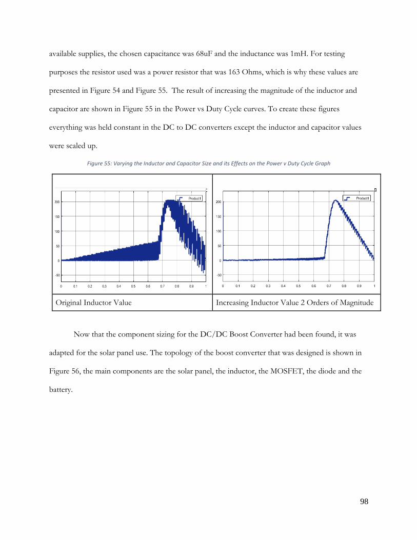
98

available supplies, the chosen capacitance was 68uF and the inductance was 1mH. For testing

purposes the resistor used was a power resistor that was 163 Ohms, which is why these values are

presented in Figure 54 and Figure 55. The result of increasing the magnitude of the inductor and

capacitor are shown in Figure 55 in the Power vs Duty Cycle curves. To create these figures

everything was held constant in the DC to DC converters except the inductor and capacitor values

were scaled up.

Figure 55: Varying the Inductor and Capacitor Size and its Effects on the Power v Duty Cycle Graph

Original Inductor Value Increasing Inductor Value 2 Orders of Magnitude

Now that the component sizing for the DC/DC Boost Converter had been found, it was

adapted for the solar panel use. The topology of the boost converter that was designed is shown in

Figure 56, the main components are the solar panel, the inductor, the MOSFET, the diode and the

battery.

99

Figure 56: Solar Charging Boost Converter Topology

In this real implementation the voltage source was replaced for the solar panel, the resistor

and capacitor was replaced for a 7.4 Volt Battery, and the last things to select were the MOSFET

and the diode that were able to meet the demands of the circuit. Because up to 340mA and 2.2

Watts could flow through the diode, a diode which was rated for those conditions needed to be

used. The IN817 diode is rated for a current up to 1A and voltage up to 20V what it is reverse

biased; additionally this diode is typically used in switching power supplies and has a low forward

voltage drop (Diodes Incorporated, ND). For the MOSFET important considerations were that the

drain to source voltage was small and that the gate be able to be triggered by a 3.3 Volt wave, this

was satisfied by the IRL2703 N-MOS (International Rectifier, ND).

In summary, maximum power point tracking is driven by the use of DC/DC converters

which act as dynamical optimizators because of their ability to change the operating point of a solar

panel through adjusting the duty cycle on the PWM pin. The parts selected to be used for the

DC/DC converter were the inductor, diode and the MOSFET.

6.3 Sensing Solar Panel Voltage, Current, Power

In order to accomplish maximum power point tracking, the voltage and current of the solar

panel must to be monitored in order to interpret the power. In this way previous values for the

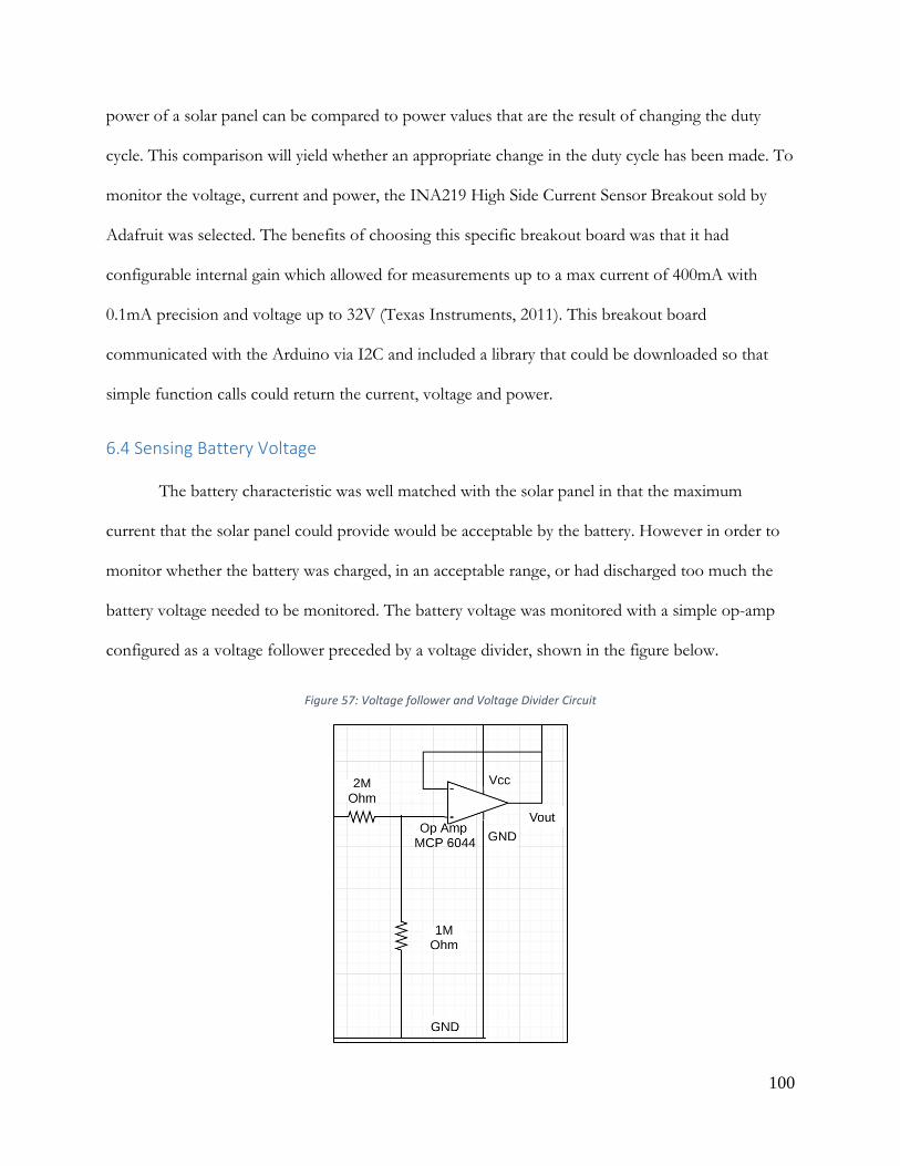
100

power of a solar panel can be compared to power values that are the result of changing the duty

cycle. This comparison will yield whether an appropriate change in the duty cycle has been made. To

monitor the voltage, current and power, the INA219 High Side Current Sensor Breakout sold by

Adafruit was selected. The benefits of choosing this specific breakout board was that it had

configurable internal gain which allowed for measurements up to a max current of 400mA with

0.1mA precision and voltage up to 32V (Texas Instruments, 2011). This breakout board

communicated with the Arduino via I2C and included a library that could be downloaded so that

simple function calls could return the current, voltage and power.

6.4 Sensing Battery Voltage

The battery characteristic was well matched with the solar panel in that the maximum

current that the solar panel could provide would be acceptable by the battery. However in order to

monitor whether the battery was charged, in an acceptable range, or had discharged too much the

battery voltage needed to be monitored. The battery voltage was monitored with a simple op-amp

configured as a voltage follower preceded by a voltage divider, shown in the figure below.

Figure 57: Voltage follower and Voltage Divider Circuit

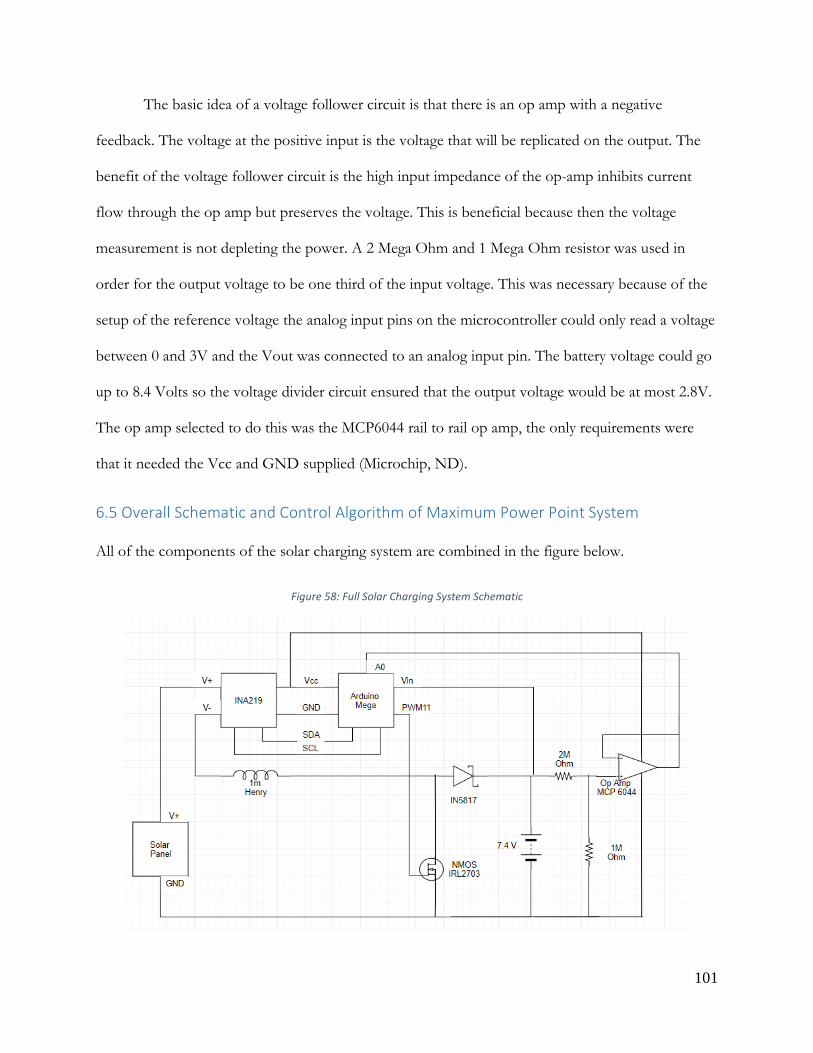
101

The basic idea of a voltage follower circuit is that there is an op amp with a negative

feedback. The voltage at the positive input is the voltage that will be replicated on the output. The

benefit of the voltage follower circuit is the high input impedance of the op-amp inhibits current

flow through the op amp but preserves the voltage. This is beneficial because then the voltage

measurement is not depleting the power. A 2 Mega Ohm and 1 Mega Ohm resistor was used in

order for the output voltage to be one third of the input voltage. This was necessary because of the

setup of the reference voltage the analog input pins on the microcontroller could only read a voltage

between 0 and 3V and the Vout was connected to an analog input pin. The battery voltage could go

up to 8.4 Volts so the voltage divider circuit ensured that the output voltage would be at most 2.8V.

The op amp selected to do this was the MCP6044 rail to rail op amp, the only requirements were

that it needed the Vcc and GND supplied (Microchip, ND).

6.5 Overall Schematic and Control Algorithm of Maximum Power Point System All of the components of the solar charging system are combined in the figure below.

Figure 58: Full Solar Charging System Schematic

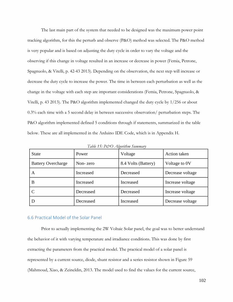
102

The last main part of the system that needed to be designed was the maximum power point

tracking algorithm, for this the perturb and observe (P&O) method was selected. The P&O method

is very popular and is based on adjusting the duty cycle in order to vary the voltage and the

observing if this change in voltage resulted in an increase or decrease in power (Femia, Petrone,

Spagnuolo, & Vitelli, p. 42-43 2013). Depending on the observation, the next step will increase or

decrease the duty cycle to increase the power. The time in between each perturbation as well as the

change in the voltage with each step are important considerations (Femia, Petrone, Spagnuolo, &

Vitelli, p. 43 2013). The P&O algorithm implemented changed the duty cycle by 1/256 or about

0.3% each time with a 5 second delay in between successive observation/ perturbation steps. The

P&O algorithm implemented defined 5 conditions through if statements, summarized in the table

below. These are all implemented in the Arduino IDE Code, which is in Appendix H.

Table 15: P&O Algorithm Summary

State Power Voltage Action taken

Battery Overcharge Non- zero 8.4 Volts (Battery) Voltage to 0V

A Increased Decreased Decrease voltage

B Increased Increased Increase voltage

C Decreased Decreased Increase voltage

D Decreased Increased Decrease voltage

6.6 Practical Model of the Solar Panel

Prior to actually implementing the 2W Voltaic Solar panel, the goal was to better understand

the behavior of it with varying temperature and irradiance conditions. This was done by first

extracting the parameters from the practical model. The practical model of a solar panel is

represented by a current source, diode, shunt resistor and a series resistor shown in Figure 59

(Mahmoud, Xiao, & Zeineldin, 2013. The model used to find the values for the current source,

103

shunt resistor, and series resistor was created by Mahmoud, Xiao, and Zeineldin and it strictly uses

the data sheet values from the solar panel. Parameterization was done using the Newton Raphson

approach to find Rs and Rsh and then the Is (short circuit current) and Ipho (photon current) could

be determined.. The two equations used for the Newtown Raphson equation that resulted in finding

Rs and Rsh are shown below and the script they are used in is in Appendix I: MATLAB Practical

Model Parameter Extraction Code.

= 0 (63)

(64)

Here q is the electron charge, K is the Boltzmann constant, T is the Temperature of the module, Ns

is the number of series cells, Iph is the photon current, I s is the saturation current, A is the ideality

factor, Rs is the series resistance, Rsh is the shunt resistor, Im is the peak power current, Vm is the

peak power voltage, and Voc is the open circuit voltage (Mahmoud, Xiao, & Zeineldin, 2013).

Figure 59: Solar Panel Practical Model

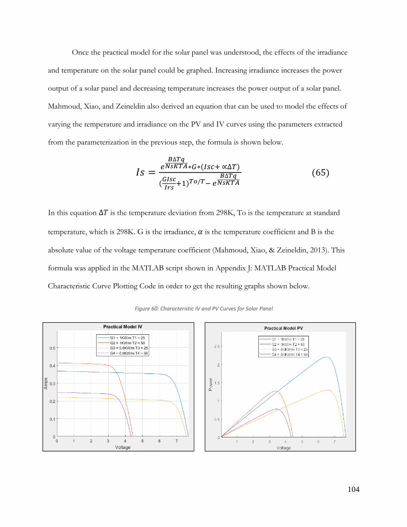
104

Once the practical model for the solar panel was understood, the effects of the irradiance

and temperature on the solar panel could be graphed. Increasing irradiance increases the power

output of a solar panel and decreasing temperature increases the power output of a solar panel.

Mahmoud, Xiao, and Zeineldin also derived an equation that can be used to model the effects of

varying the temperature and irradiance on the PV and IV curves using the parameters extracted

from the parameterization in the previous step, the formula is shown below.

𝐼𝐼𝐿𝐿 = 𝑒𝑒𝐿𝐿∆𝑇𝑇𝑇𝑇𝑁𝑁𝑁𝑁𝑁𝑁𝑇𝑇𝑁𝑁∗𝐺𝐺∗(𝐼𝐼𝑠𝑠𝐼𝐼+ ∝∆𝑇𝑇)

(𝐺𝐺𝐺𝐺𝑁𝑁𝐺𝐺𝐺𝐺𝐼𝐼𝑁𝑁 +1)𝑇𝑇𝑇𝑇/𝑇𝑇− 𝑒𝑒𝐿𝐿∆𝑇𝑇𝑇𝑇𝑁𝑁𝑁𝑁𝑁𝑁𝑇𝑇𝑁𝑁

(65)

In this equation ∆𝑇𝑇 is the temperature deviation from 298K, To is the temperature at standard

temperature, which is 298K. G is the irradiance, 𝛼𝛼 is the temperature coefficient and B is the

absolute value of the voltage temperature coefficient (Mahmoud, Xiao, & Zeineldin, 2013). This

formula was applied in the MATLAB script shown in Appendix J: MATLAB Practical Model

Characteristic Curve Plotting Code in order to get the resulting graphs shown below.

Figure 60: Characteristic IV and PV Curves for Solar Panel

105

6.7 Simulation of the Solar Charging System

After understanding the model of the solar panel itself and the DC/DC Boost Converter,

both were combined in a MATLAB Simulink Model. The model is shown in Appendix K:

MATLAB Simulink Practical Model Solar Panel with DC/DC Converter and the code for the

maximum power point tracking algorithm used in the model is in Appendix L: Maximum Power

Point Tracking Code written in MATLAB. The Simulink model was used in order to verify the

operation of the entire system. It was also used to adjust the parameters within the model and

observe their effects on the output. One test that was done in Simulink was looking at the tradeoffs

of increasing or decreasing the duty cycle step size. Two different duty cycle step sizes are shown in

the figure below along with their Voltage vs Time curves, the change in the voltage is the result of

the P&O algorithm searching for the new maximum power voltage operating point as a result of

temperature increase and irradiance decrease (when the voltage went down) and temperature

decrease and irradiance increase (when the voltage went back up).

Figure 61: Effect of Duty Cycle Step Size on Maximum Power Point Tracking

Duty Cycle Step 0.05 Duty Cycle Step 0.01

The notable observation from these graphs is that there is a tradeoff between the speed it

takes to reach the maximum power and the oscillations around the maximum power once the

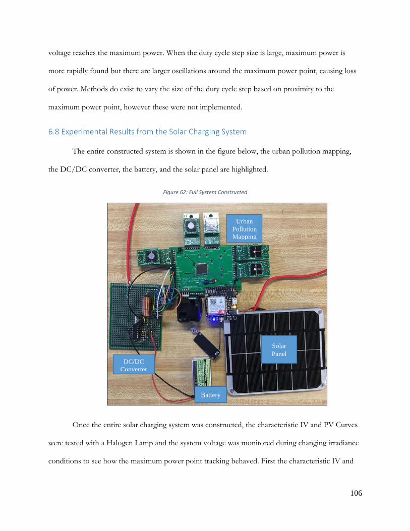
106

voltage reaches the maximum power. When the duty cycle step size is large, maximum power is

more rapidly found but there are larger oscillations around the maximum power point, causing loss

of power. Methods do exist to vary the size of the duty cycle step based on proximity to the

maximum power point, however these were not implemented.

6.8 Experimental Results from the Solar Charging System

The entire constructed system is shown in the figure below, the urban pollution mapping,

the DC/DC converter, the battery, and the solar panel are highlighted.

Figure 62: Full System Constructed

Once the entire solar charging system was constructed, the characteristic IV and PV Curves

were tested with a Halogen Lamp and the system voltage was monitored during changing irradiance

conditions to see how the maximum power point tracking behaved. First the characteristic IV and

Urban Pollution Mapping

Solar Panel

Battery

DC/DC Converter

107

PV curves were created by writing a MATLAB code that stepped through all of the possible duty

cycles and the current, voltage and power of the solar panel were monitored. The characteristic

curves are shown in the Figure 63.

Figure 63: The IV and PV Characteristic Curves for the Solar Panel

Due to the solar panel characteristics being tested under a Halogen light, the full power was

not seen in the testing. However, the main goal of the duty cycle sweeping test was to ensure that

the correct shape for the IV and PV curves were realized and they successfully were.

Next, the solar panels efforts to reach maximum power were observed. The figure below

shows successive steps where with each step 1-6 the power output increased, however from 6- 7 the

power decreased with an increase in the voltage so for the next step, 7-8, the voltage was decreased

in order for it to recover its power, then in the last step 8-9 the voltage was decreased again to lead

to a higher power output.

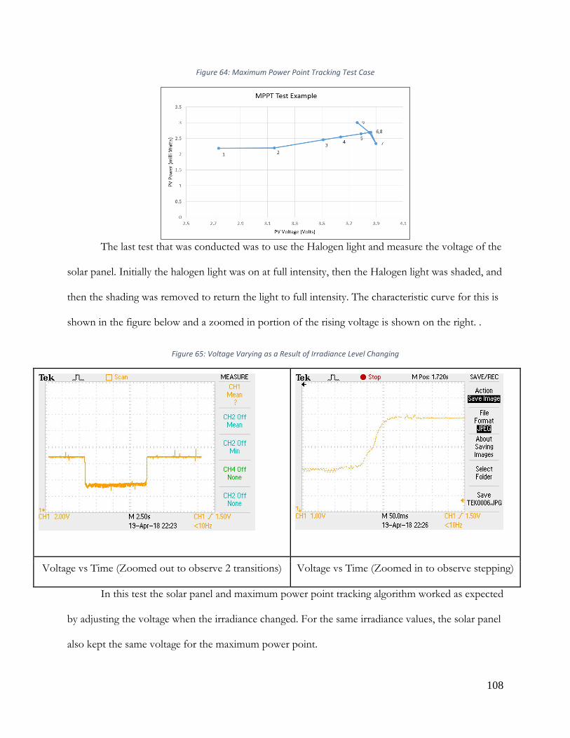
108

Figure 64: Maximum Power Point Tracking Test Case

The last test that was conducted was to use the Halogen light and measure the voltage of the

solar panel. Initially the halogen light was on at full intensity, then the Halogen light was shaded, and

then the shading was removed to return the light to full intensity. The characteristic curve for this is

shown in the figure below and a zoomed in portion of the rising voltage is shown on the right. .

Figure 65: Voltage Varying as a Result of Irradiance Level Changing

Voltage vs Time (Zoomed out to observe 2 transitions) Voltage vs Time (Zoomed in to observe stepping)

In this test the solar panel and maximum power point tracking algorithm worked as expected

by adjusting the voltage when the irradiance changed. For the same irradiance values, the solar panel

also kept the same voltage for the maximum power point.

109

6.9 Recommendations for Future Work Overall, the solar charging system was designed and implemented in order to provide the

power system to the Urban Pollution Mapping device. Improvements to the system could certainly

be made. The main areas that could be improved based on this project is the selection of the solar

panel and the battery. Theoretically the selections were valid however practically the battery actually

discharged rapidly. A solar panel that is rated for faster charging and a higher capacity battery would

improve the project’s success. Another improvement could be made would be by adjusting the

maximum power point tracking algorithm. More duty cycle step sizes and wait times could be tested

in order to select the best options for the system. The last improvement recommended is combining

the urban pollution mapping subsystem and the solar charging subsystem into one printed circuit

board to make the system a single packaged version.

110

References Chapters 1-5 American Building Components - Metal Roofing & Wall Panel Colors. (n.d.). Retrieved March 21,

2018, from http://abcmetalroofing.chameleonpower.com/ Bhargav, M. M. S. R. S., Ratna Kishore, V., Anbuudayasankar, S. P., & Balaji, K. (2016). Power

generation by high head water in a building using micro hydro turbine—a greener approach. Environmental Science and Pollution Research, 23(10), 9381–9390. https://doi.org/10.1007/s11356-015-5317-6

Cobb, B. R., & Sharp, K. V. (2013). Impulse (Turgo and Pelton) turbine performance characteristics

and their impact on pico-hydro installations. Renewable Energy, 50, 959–964. https://doi.org/10.1016/j.renene.2012.08.010

“Comparison between Impulse Turbine and Reaction Turbine” (2016). Retrieved October 14, 2017,

from https://me-mechanicalengineering.com/comparison-between-impulse-turbine-and-reactionturbine/

Gkavanasios, J. (2017, September 18). Pelton Turbine[SolidWorks Part]. GrabCad. Golder Associates. (2012). Liberty, N. E. W., Mine, G., Environmental, P., & Statement, I. Section

B: Surface Water Assessment Report. González-Eguino, M. (2015). Energy poverty: An overview. Renewable and Sustainable Energy

Reviews, 47, 377–385. https://doi.org/10.1016/j.rser.2015.03.013 Green Energy. (n.d.). Retrieved March 21, 2018, from http://www.partnerliberia.org International Energy Outlook, IEO2017 (September 14, 2017). Kanth, B. P., Ashwani., & Sharma, S. (2012). House Hold Power Generation Using Rain Water. The

International Journal of Engineering, 1(2), 77–80. Retrieved from www.theijes.com Liberia Institute of Statistics and Geo-Information Services. (2013). Liberia Demographic and

Health Survey 2013, 480. Retrieved from http://dhsprogram.com/publications/publication-fr291-dhsfinal-reports.cfm

Munson, B., Okiishi, T., Huebsch, W., Rothmayer, A. (2013). Fundamentals of Fluid Mechanics.

Hoboken, NJ: John Wiley & Sons. Okot, D. K. (2013). Review of small hydropower technology. Renewable and Sustainable Energy

Reviews, 26, 515-520. https://doi.org/10.1016/j.rser.2013.05.006 Quaranta, E., & Revelli, R. (2015). Output power and power losses estimation for an overshot water

wheel. Renewable Energy,83, 979-987. doi:10.1016/j.renene.2015.05.018 SHAH, Q. (2014, October 8). CrossFlow turbine[SolidWorks Part]. GrabCad.

http://abcmetalroofing.chameleonpower.com/

https://doi.org/10.1007/s11356-015-5317-6

https://doi.org/10.1016/j.renene.2012.08.010

https://me-mechanicalengineering.com/comparison-between-impulse-turbine-and-reactionturbine/

https://me-mechanicalengineering.com/comparison-between-impulse-turbine-and-reactionturbine/

https://doi.org/10.1016/j.rser.2015.03.013

http://www.partnerliberia.org/

http://www.theijes.com/

http://dhsprogram.com/publications/publication-fr291-dhsfinal-reports.cfm

http://dhsprogram.com/publications/publication-fr291-dhsfinal-reports.cfm


111

SMACNA. (2012). Architectural Sheet Metal Manual: Technical Publication. Chantilly, VA: Author. Still, G., & Thomas, T. (2002, December). THE OPTIMUM SIZING OF GUTTERS FOR

DOMESTIC ROOFWATER HARVESTING(Rep.). Retrieved March 21, 2018, from University of Warwick website: https://warwick.ac.uk/fac/sci/eng/research/grouplist/structural/dtu/pubs/wp/wp56/wp56.pdf

Stram, B. N. (2016). Key challenges to expanding renewable energy. Energy Policy, 96, 728–734.

https://doi.org/10.1016/j.enpol.2016.05.034 Tester, J., Drake, E., Driscoll, M., Golay, M., & Peters, W. (2016). Sustainable Energy: Choosing

Among Options (2nd ed.). Cambridge, MA: The MIT Press. Understanding D.C. Motor Characteristics. (n.d.). Retrieved March 21, 2018, from

http://lancet.mit.edu/motors/motors3.html United Nations Development Programme. (2016). Human Development Report 2016. United

Nations Development Programme. https://doi.org/eISBN: 978-92-1-060036-1 Urmee, T., & Md, A. (2016). Social, cultural and political dimensions of off-grid renewable energy

programs in developing countries, 93, 159–167. https://doi.org/10.1016/j.renene.2016.02.040

V. (2015, April 10). Waterwheel [SolidWorks Part]. GrabCad. Vieira, A. S., Beal, C. D., Ghisi, E., & Stewart, R. A. (2014). Energy intensity of rainwater harvesting

systems: A review. Renewable and Sustainable Energy Reviews, 34, 225–242. https://doi.org/10.1016/j.rser.2014.03.012

Waterwheel Design and the Different Types of Waterwheel. (2013). Retrieved October 14, 2017, from http://www.alternative-energy-tutorials.com/hydro-energy/waterwheel-design.html

World Energy Council. (2016). World Energy Resources 2016. 1-1028. Retrieved from

https://www.worldenergy.org/wp-content/uploads/2016/10/World-Energy-Resources-Full-report-2016.10.03.pdf.

WIN, Z., WIN, H., & THEIN, M. (2016). DESIGN, CONSTRUCTION AND PERFORMANCE

TEST OF CROSS-FLOW TURBINE. International Journal of Mechanical And Production Engineering,,4(12), 95-100.

Williamson, S. J., Stark, B. H., & Booker, J. D. (2014). Low head pico hydro turbine selection using a

multicriteria analysis. Renewable Energy, 61, 43–50. https://doi.org/10.1016/j.renene.2012.06.020

https://doi.org/10.1016/j.renene.2016.02.040


http://www.alternative-energy-tutorials.com/hydro-energy/waterwheel-design.html

https://www.worldenergy.org/wp-content/uploads/2016/10/World-Energy-Resources-Full-report-2016.10.03.pdf

https://www.worldenergy.org/wp-content/uploads/2016/10/World-Energy-Resources-Full-report-2016.10.03.pdf

112

Wu, W., Geng, P., Li, G., Zhau, D., Zhang, H., & Zhao, J. (2015). Influence of Layer Thickness and Raster Angle on the Mechnical Properties of 3D-Printed PEEK and a Comparative

Mechanical Study between PEEK and ABS. Materials, 8(9), 5834-5846. Doi:10.3390/ma8095271

Zhou, D., & Deng, Z. (Daniel). (2017). Ultra-low-head hydroelectric technology: A review. Renewable and Sustainable Energy Reviews, 78(March 2016), 23–30. https://doi.org/10.1016/j.rser.2017.04.086

Židonis, A., & Aggidis, G. A. (2016). Pelton turbine: Identifying the optimum number of buckets

using CFD. Journal of Hydrodynamics, Ser. B,28(1), 75-83. doi:10.1016/s1001-6058(16)60609-1

References Chapter 6 Diodes Incorporated. (ND). 1N5817 - 1N5819 1.0A Schottky Barrier Rectifier [Data Sheet] Retrieved from https://www.diodes.com/assets/Datasheets/ds23001.pdf April 24, 2018. Femia, N., Petrone, G., Spagnuolo, G., & Vitelli, M. (2013). Power electronics and control techniques for maximum energy harvesting in photovoltaic systems. CRC Press, Taylor & Francis Group. GN Batteries & Electronics, Inc. (July 30, 2011). RLI-9720 Li-Ion Polymer Battery Pack [Data Sheet] Retrieved from https://www.batterymart.com/pdfs/rli-9720.pdf April 24, 2018. International Rectifier. (ND). IRL2703 HEXFET Power MOSFET [Data Sheet] Retrieved from http://www.engr.usask.ca/classes/EE/204/labs/IRL2703_FET.pdf April 24, 2018. Mahmoud, Y. A., Xiao, W., & Zeineldin, H. H. (2013). A parameterization approach for enhancing PV model accuracy. IEEE Transactions on Industrial Electronics, 60(12), 5708-5716. doi:10.1109/TIE.2012.2230606 Microchip. (ND). MCP6041/2/3/4 600nA, Rail-to-Rail Input/Output Op Amps [Data Sheet] Retrieved from http://ww1.microchip.com/downloads/en/DeviceDoc/21669D.pdf April 24, 2018. Mohan, N., Undeland, T. M., & Robbins, W. P. (2003). Power electronics: Converters, applications, and design (3rd ed.). Hoboken, NJ: John Wiley & Sons. Texas Instruments. (August 2008. Revised September 2011). Zero Drift, Bi-Directional Current/Power Monitor with I2C Interface [Data Sheet] Retrieved from https://cdn-shop.adafruit.com/datasheets/ina219.pdf April 24, 2018. Voltaic Systems. (July 24, 2017). 2W 6V 112x136 mm Solar Panel [Data Sheet] Retrieved from https://www.voltaicsystems.com/2-watt-panel April 24, 2018.


https://www.diodes.com/assets/Datasheets/ds23001.pdf

https://www.batterymart.com/pdfs/rli-9720.pdf

http://www.engr.usask.ca/classes/EE/204/labs/IRL2703_FET.pdf

http://ww1.microchip.com/downloads/en/DeviceDoc/21669D.pdf

https://cdn-shop.adafruit.com/datasheets/ina219.pdf

https://www.voltaicsystems.com/2-watt-panel

113

Voltaic Systems. (ND). Small Solar Panels. Retrieved from https://www.voltaicsystems.com/solar-panels April 24, 2018.

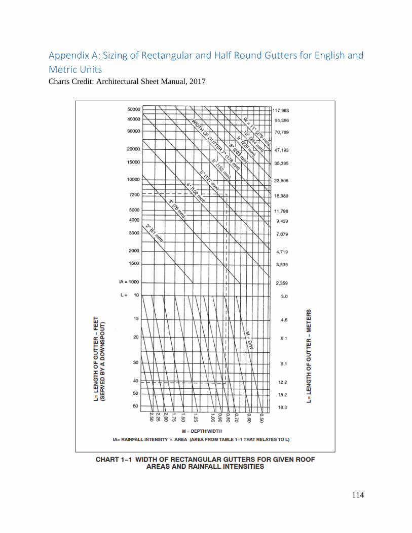
https://www.voltaicsystems.com/solar-panels

114

Appendix A: Sizing of Rectangular and Half Round Gutters for English and Metric Units Charts Credit: Architectural Sheet Manual, 2017

116

Appendix B: Overshot Water Wheel Assembly Drawings

117

Appendix C: Pelton Wheel Assembly Drawings

118

Appendix D: Crossflow Turbine Assembly Drawings

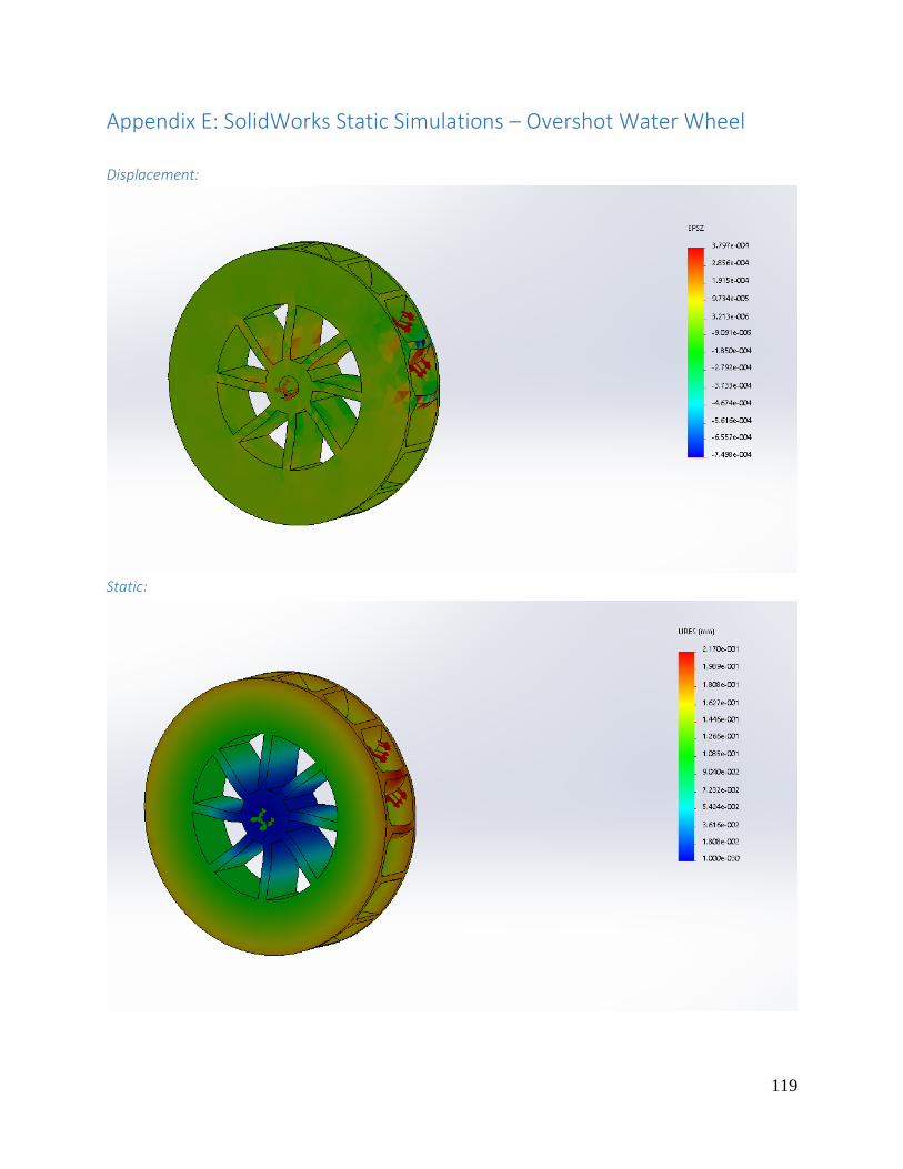
119

Appendix E: SolidWorks Static Simulations – Overshot Water Wheel Displacement:

Static:

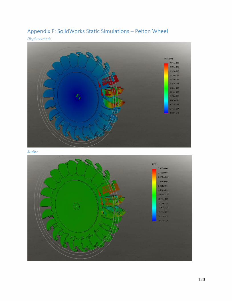
120

Appendix F: SolidWorks Static Simulations – Pelton Wheel Displacement:

Static:

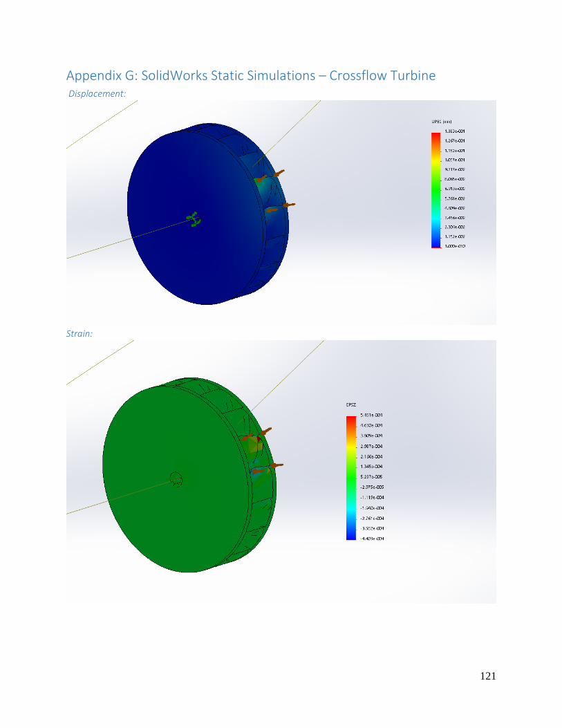
121

Appendix G: SolidWorks Static Simulations – Crossflow Turbine Displacement:

Strain:

122

Appendix H: Arduino IDE MPPT Code #include <Wire.h> #include <Adafruit_INA219.h> Adafruit_INA219 ina219_PV; //Adafruit_INA219 ina219_Battery(0x41); int pin = 11; void setup(void) { int myEraser = 7; // this is 111 in binary and is used as an eraser TCCR1B &= ~myEraser; // this operation (AND plus NOT), set the three bits in TCCR1B to 0 int myPrescaler = 1; // this could be a number in [1 , 6]. In this case, 3 corresponds in binary to 011. TCCR1B |= myPrescaler; //this operation (OR), replaces the last three bits in TCCR2B with our new value 011 Serial.begin(115200); while (!Serial) { // will pause Zero, Leonardo, etc until serial console opens delay(1); } analogReference(EXTERNAL); Serial.println("Hello!"); // Initialize the INA219. // By default the initialization will use the largest range (32V, 2A). However // you can call a setCalibration function to change this range (see comments). ina219_PV.begin(); //ina219_Battery.begin(); // To use a slightly lower 32V, 1A range (higher precision on amps): //ina219.setCalibration_32V_1A(); // Or to use a lower 16V, 400mA range (higher precision on volts and amps): ina219_PV.setCalibration_16V_400mA(); //ina219_Battery.setCalibration_16V_400mA(); Serial.println("Setup complete"); } void loop(void) { float Power; float Old_Power;

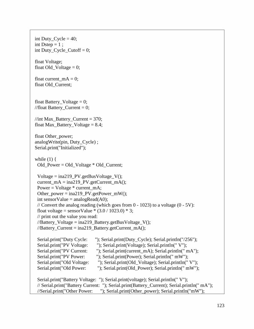
123

int Duty_Cycle = 40; int Dstep = 1 ; int Duty_Cycle_Cutoff = 0; float Voltage; float Old_Voltage = 0; float current_mA = 0; float Old_Current; float Battery_Voltage = 0; //float Battery_Current = 0; //int Max_Battery_Current = 370; float Max_Battery_Voltage = 8.4; float Other_power; analogWrite(pin, Duty_Cycle) ; Serial.print("Initialized"); while (1) { Old_Power = Old_Voltage * Old_Current; Voltage = ina219_PV.getBusVoltage_V(); current_mA = ina219_PV.getCurrent_mA(); Power = Voltage * current_mA; Other_power = ina219_PV.getPower_mW(); int sensorValue = analogRead(A0); // Convert the analog reading (which goes from 0 - 1023) to a voltage (0 - 5V): float voltage = sensorValue * (3.0 / 1023.0) * 3; // print out the value you read: //Battery_Voltage = ina219_Battery.getBusVoltage_V(); //Battery_Current = ina219_Battery.getCurrent_mA(); Serial.print("Duty Cycle: "); Serial.print(Duty_Cycle); Serial.println("/256"); Serial.print("PV Voltage: "); Serial.print(Voltage); Serial.println(" V"); Serial.print("PV Current: "); Serial.print(current_mA); Serial.println(" mA"); Serial.print("PV Power: "); Serial.print(Power); Serial.println(" mW"); Serial.print("Old Voltage: "); Serial.print(Old_Voltage); Serial.println(" V"); Serial.print("Old Power: "); Serial.print(Old_Power); Serial.println(" mW"); Serial.print("Battery Voltage: "); Serial.print(voltage); Serial.println(" V"); // Serial.print("Battery Current: "); Serial.print(Battery_Current); Serial.println(" mA"); //Serial.print("Other Power: "); Serial.print(Other_power); Serial.println("mW");

124

if ((Battery_Voltage > Max_Battery_Voltage){ Duty_Cycle = Duty_Cycle_Cutoff; Serial.println("Battery Fail Condition"); } //Increasing power, Increasing Voltage //keep increasing volgate by decreasing duty cycle if (Duty_Cycle < 0){ Duty_Cycle = 10; //resetting up a little higher to prevent negative } if ((Power > Old_Power) and (Voltage > Old_Voltage)) { Duty_Cycle = Duty_Cycle - Dstep; Serial.println("A"); } //Increasing power, Decreasing Voltage //keep decreasing volgate by increasing duty cycle else if ((Power >= Old_Power) and (Voltage <= Old_Voltage)) { Duty_Cycle = Duty_Cycle + Dstep; Serial.println("B"); } //Decreasing power, Increasing Voltage //instead decrease volgate by increasing duty cycle else if ((Power < Old_Power) and (Voltage >= Old_Voltage)) { Duty_Cycle = Duty_Cycle + Dstep; Serial.println("C"); } //Decreasing power, Decreasing Voltage //instead increase volgate by decreasing duty cycle else if ((Power < Old_Power) and (Voltage <= Old_Voltage)) { Duty_Cycle = Duty_Cycle - Dstep; Serial.println("D"); } analogWrite(pin, Duty_Cycle) ;// use pins 12 or 11 Serial.println(""); //set the olds Old_Power = Power; Old_Voltage = Voltage; Old_Current = current_mA; delay(5000); } }

125

Appendix I: MATLAB Practical Model Parameter Extraction Code

%Practical PV model %Parameters Iph, Is, Rs, and Rsh are found through 4 equations and A is %assumed to be 1.3 %CURRENT AND VOLTAGE FROM IN CLASS EXAMPLE PV MODULE function F = solving(x) %constants q = 1.60217657e-19; K = 1.3806488e-23; Voc = 7.7; Vm = 6.5; Isc = 0.370; Im = 0.340; Ns = 12; T = 25+273; A = .7; %define variables to be solved using the Newton Raphson equations Rs = x(1); Rsh = x(2); F(1)=Isc-Im-(Vm+Im*Rs)/Rsh-(Isc-Voc/Rsh)*(exp(q*(Vm+Im*Rs)/(Ns*K*T*A))-1)/(exp(q*Voc/(Ns*K*T*A))-1) ; F(2)= exp(q*(Vm+Im*Rs)/(Ns*K*T*A))*(q*Im*Rs*Voc/(Ns*K*T*A*Vm*Rsh)-q*Im*Rs*Isc/(Ns*K*T*A*Vm)-q*Voc/(Ns*K*T*A*Rsh)+q*Isc/(Ns*K*T*A))/(exp(q*Voc/(Ns*K*T*A))-1)-Im/Vm-Im*Rs/(Rsh*Vm)+1/Rsh; %printing of all the values Rs Rsh Ipho = Isc Iso = (Ipho-(Voc/Rsh))/((exp((q*Voc)/(Ns*K*T*A))-1)) end

126

Appendix J: MATLAB Practical Model Characteristic Curve Plotting Code

%Practical model %Plots of IV and PV curves at various conditions for given G and T %Parameters taken from Assig1_Practical_Model Rs = 0.5274; Rsh =331.8286; Ipho = 8.2300; Iso = 8.3538e-15; %constants q = 1.60217657e-19; K = 1.3806488e-23; Voc = 33.5; Vm = 26.3; Isc = 8.23; Im = 7.8; Ns = 54; T = 25+273; A = .7; alpha = 0.5/100*Isc; B = -0.116; %G1 = 1KW/m T1 = 25 G1= 1; T1 = 25 + 273; Iph1 = G1*(Ipho+alpha*(T1-T)); Is1 = Ipho/(exp(q*(Voc - (abs(B)*(T1-T)))/(Ns*K*T1*A))-1); %G2 = 1KW/m T2 = 50 G2 = 1; T2 = 50+ 273; Iph2 = G2*(Ipho+alpha*(T2-T)); Is2 = Ipho/(exp(q*(Voc - (abs(B)*(T2-T)))/(Ns*K*T2*A))-1); %G3 = 0.6KW/m T3 = 25 G3 = 0.6; T3 = 25+ 273; Iph3 = G3*(Ipho+alpha*(T3-T)); Is3 = Ipho/(exp(q*(Voc - (abs(B)*(T3-T)))/(Ns*K*T3*A))-1); %G4 = 0.6KW/m T3 = 50 G4 = 0.6; T4 = 50+ 273; Iph4 = G4*(Ipho+alpha*(T4-T)); Is4 = Ipho/(exp(q*(Voc - (abs(B)*(T4-T)))/(Ns*K*T4*A))-1); %plotting the results X = 0: .1: Voc; syms C; c = 8; for i = 1:length(X) %use Newton - Raphson method to find current F(C) = Iph1 - C- Is1*((exp((q*(X(i)+ C*Rs))/(Ns*K*T*A))-1)) - (X(i)+ C*Rs)/Rsh ; Fd(C) = diff(F(C));

127

ans1 = double(F(c)); ans2 = double(Fd(c)); while abs(ans1) > 1e-6 c = double(c - ans1/ans2); ans1 = double(F(c)); ans2 = double(Fd(c)); end I1(i) = c; P1(i) = c * X(i); end syms D; d = 8; for i = 1:length(X) %use Newton - Raphson method to find current F(D) = Iph2 - D- Is2*((exp((q*(X(i)+ D*Rs))/(Ns*K*T*A))-1)) - (X(i)+ D*Rs)/Rsh ; Fd(D) = diff(F(D)); ans1 = double(F(d)); ans2 = double(Fd(d)); while abs(ans1) > 1e-6 d = double(d - ans1/ans2); ans1 = double(F(d)); ans2 = double(Fd(d)); end I2(i) = d; P2(i) = d * X(i); end syms D; d = 4; for i = 1:length(X) %use Newton - Raphson method to find current F(D) = Iph3 - D- Is3*((exp((q*(X(i)+ D*Rs))/(Ns*K*T*A))-1)) - (X(i)+ D*Rs)/Rsh ; Fd(D) = diff(F(D)); ans1 = double(F(d)); ans2 = double(Fd(d)); while abs(ans1) > 1e-6 d = double(d - ans1/ans2); ans1 = double(F(d)); ans2 = double(Fd(d)); end I3(i) = d; P3(i) = d * X(i); end syms D; d = 8; for i = 1:length(X) %use Newton - Raphson method to find current F(D) = Iph4 - D- Is4*((exp((q*(X(i)+ D*Rs))/(Ns*K*T*A))-1)) - (X(i)+ D*Rs)/Rsh ; Fd(D) = diff(F(D)); ans1 = double(F(d)); ans2 = double(Fd(d)); while abs(ans1) > 1e-6 d = double(d - ans1/ans2); ans1 = double(F(d)); ans2 = double(Fd(d)); end I4(i) = d;

128

P4(i) = d * X(i); end figure(1) hold on a1 = plot(X,I1); M1 = "G1 = 1KW/m T1 = 25"; a2 = plot(X,I2); M2 = "G2 = 1KW/m T2 = 50"; a3 = plot(X,I3); M3 = "G3 = 0.6KW/m T3 = 25"; a4 = plot(X,I4); M4 = "G4 = 0.6KW/m T4 = 50"; xlim([0 Voc]) ylim([0 10]) legend([a1,a2, a3, a4], [M1, M2, M3, M4],'Location', 'South'); title('Practical Model IV') grid on xlabel('Voltage') ylabel('Amps') hold off figure(2) hold on a1 = plot(X,P1); M1 = "G1 = 1KW/m T1 = 25"; a2 = plot(X,P2); M2 = "G2 = 1KW/m T2 = 50"; a3 = plot(X,P3); M3 = "G3 = 0.6KW/m T3 = 25"; a4 = plot(X,P4); M4 = "G4 = 0.6KW/m T4 = 50"; xlim([0 Voc]) ylim([0 250]) legend([a1,a2, a3, a4], [M1, M2, M3, M4],'Location', 'South'); title('Practical Model PV') grid on xlabel('Power') ylabel('Amps') hold off

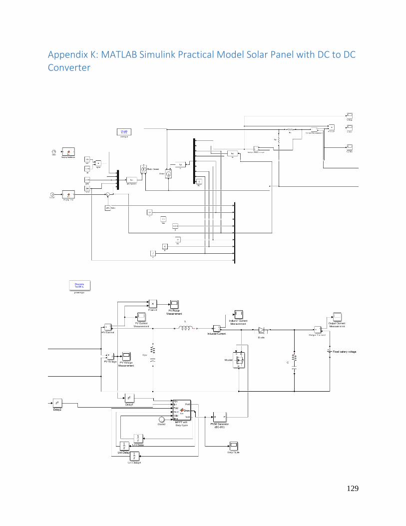
129

Appendix K: MATLAB Simulink Practical Model Solar Panel with DC to DC Converter

130

Appendix L: Maximum Power Point Tracking Code written in MATLAB

function [Pold, Dnew, Vold] = fcn(Vpv, Ipv, Pold, Dold, Vold, time) %The duty cycle actually should only range from %a maximum of 1 to a minimum of 0.665 %V = 0 at D =1 and Voc 33.5 at D = 0.665 %governing equation Vpv = Vo*(1-D) %Calculate new power using PV voltage and current Pnew = Vpv*Ipv; Dnew = 0; %because matlab and me disagree Dstep = 0.01; %Initital condition is D = 0.7 to get simulation started if time < .1 Dnew = 0.8; %Increasing power, Increasing Voltage %keep increasing volgate by decreasing duty cycle elseif (time >= .1) && (Pnew >= Pold) && (Vpv >= Vold) Dnew = Dold - Dstep; %Increasing power, Decreasing Voltage %keep decreasing volgate by increasing duty cycle elseif (time >= .1) && (Pnew >= Pold) && (Vpv <= Vold) Dnew = Dold + Dstep; %Decreasing power, Increasing Voltage %instead decrease volgate by increasing duty cycle elseif (time >= .1) && (Pnew <= Pold) && (Vpv >= Vold) Dnew = Dold + Dstep; %Decreasing power, Decreasing Voltage %instead increase volgate by decreasing duty cycle elseif (time >= .1)&& (Pnew <= Pold) && (Vpv <= Vold) Dnew = Dold - Dstep; end %set the olds Pold = Pnew; Vold = Vpv; end

Energy Harvesting from Rainwater and Maximum Power Point ... · Crossflow turbine, and Pelton wheel...

Documents

Transcript of Energy Harvesting from Rainwater and Maximum Power Point ... · Crossflow turbine, and Pelton wheel...