Energy Forecasting Methods - Purdue University -...

ENERGY CENTERState Utility Forecasting Group (SUFG)


Energy Forecasting Methods

Presented by:Douglas J. Gotham

State Utility Forecasting GroupEnergy Center

Purdue University

Presented to:Indiana Utility Regulatory Commission

Indiana Office of the Utility Consumer Counselor

November 15, 2007



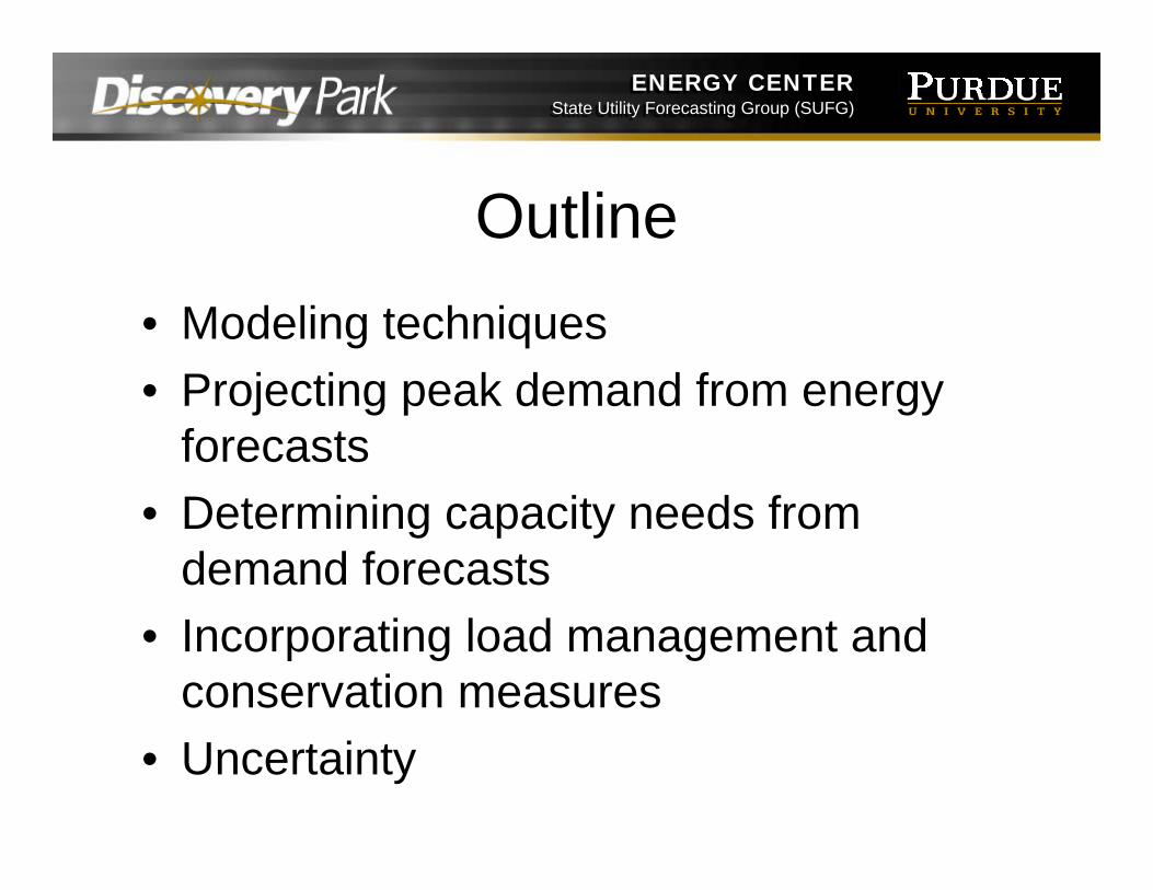
Outline• Modeling techniques• Projecting peak demand from energy

forecasts• Determining capacity needs from

demand forecasts• Incorporating load management and

conservation measures• Uncertainty



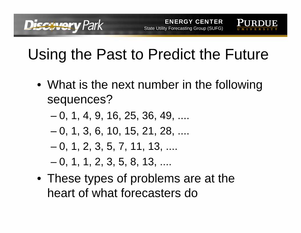
Using the Past to Predict the Future

• What is the next number in the following sequences?– 0, 1, 4, 9, 16, 25, 36, 49, ....– 0, 1, 3, 6, 10, 15, 21, 28, ....– 0, 1, 2, 3, 5, 7, 11, 13, ....– 0, 1, 1, 2, 3, 5, 8, 13, ....

• These types of problems are at the heart of what forecasters do



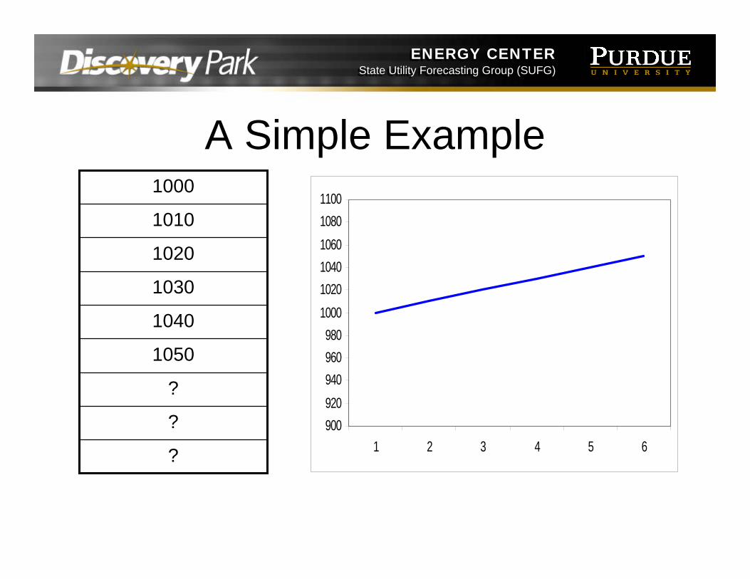
A Simple Example

900920940960980

100010201040106010801100

1 2 3 4 5 6?

?

?

1050

1040

1030

1020

1010

1000



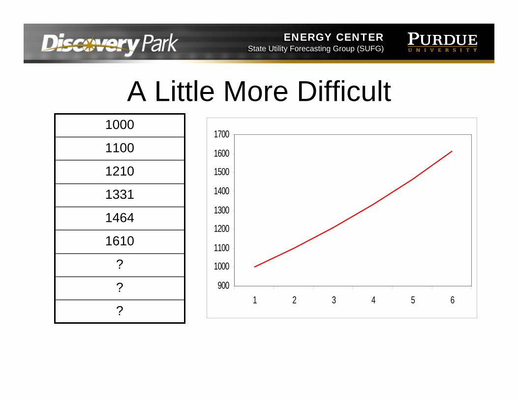
A Little More Difficult

?

?

?

1610

1464

1331

1210

1100

1000

900

1000

1100

1200

1300

1400

1500

1600

1700

1 2 3 4 5 6



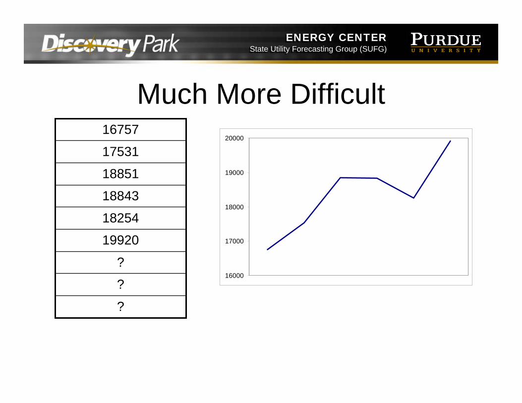
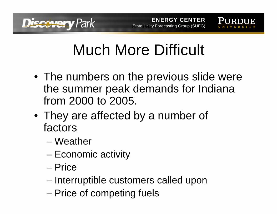
Much More Difficult

?

?

?

19920

18254

18843

18851

17531

16757

16000

17000

18000

19000

20000



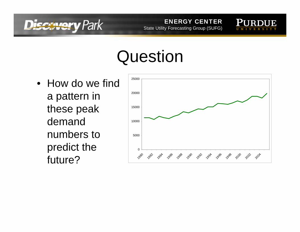
Much More Difficult• The numbers on the previous slide were

the summer peak demands for Indiana from 2000 to 2005.

• They are affected by a number of factors– Weather– Economic activity– Price– Interruptible customers called upon– Price of competing fuels



Question• How do we find

a pattern in these peak demand numbers to predict the future?

0

5000

10000

15000

20000

25000

1980

1982

1984

1986

1988

1990

1992

1994

1996

1998

2000

2002

2004



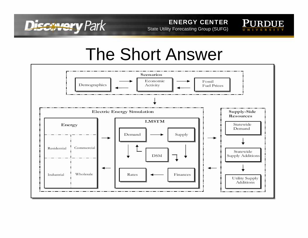
The Short Answer



Methods of Forecasting• Time Series

– trend analysis• Econometric

– structural analysis• End Use

– engineering analysis



Time Series Forecasting• Linear Trend

– fit the best straight line to the historical data and assume that the future will follow that line (works perfectly in the 1st

example)– Many methods exist for finding the best fitting line, the most

common is the least squares method.• Polynomial Trend

– Fit the polynomial curve to the historical data and assume that the future will follow that line

– Can be done to any order of polynomial (square, cube, etc) but higher orders are usually needlessly complex

• Logarithmic Trend– Fit an exponential curve to the historical data and assume

that the future will follow that line (works perfectly for the 2nd

example)



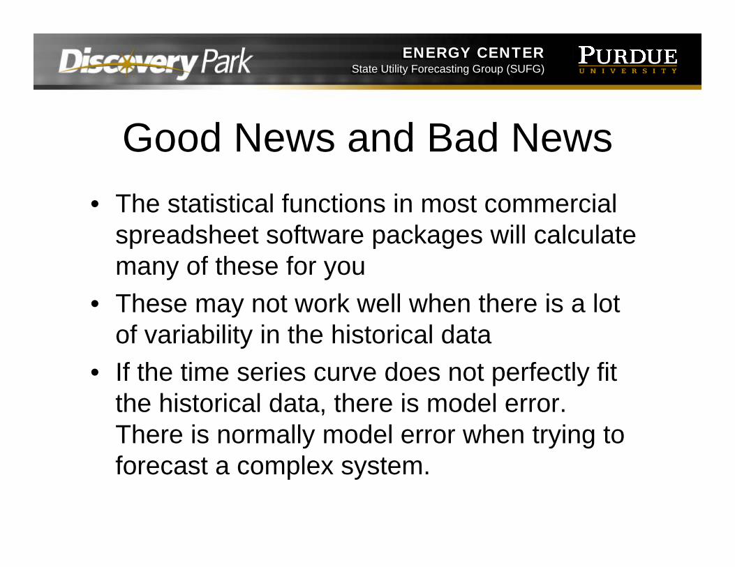
Good News and Bad News• The statistical functions in most commercial

spreadsheet software packages will calculate many of these for you

• These may not work well when there is a lot of variability in the historical data

• If the time series curve does not perfectly fit the historical data, there is model error. There is normally model error when trying to forecast a complex system.



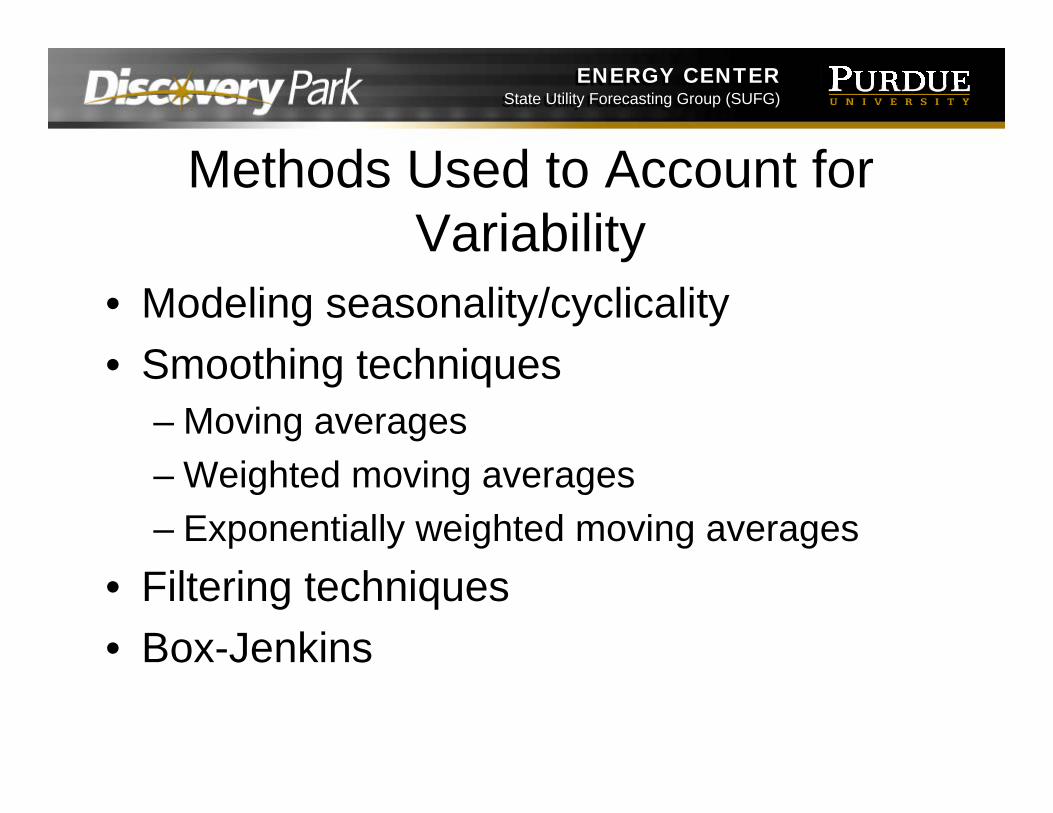
Methods Used to Account for Variability

• Modeling seasonality/cyclicality• Smoothing techniques

– Moving averages– Weighted moving averages– Exponentially weighted moving averages

• Filtering techniques• Box-Jenkins



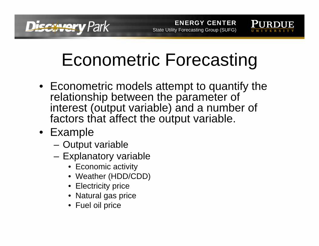
Econometric Forecasting• Econometric models attempt to quantify the

relationship between the parameter of interest (output variable) and a number of factors that affect the output variable.

• Example– Output variable– Explanatory variable

• Economic activity• Weather (HDD/CDD)• Electricity price• Natural gas price• Fuel oil price



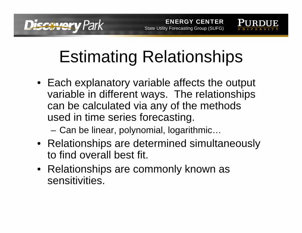
Estimating Relationships• Each explanatory variable affects the output

variable in different ways. The relationships can be calculated via any of the methods used in time series forecasting.– Can be linear, polynomial, logarithmic…

• Relationships are determined simultaneously to find overall best fit.

• Relationships are commonly known as sensitivities.



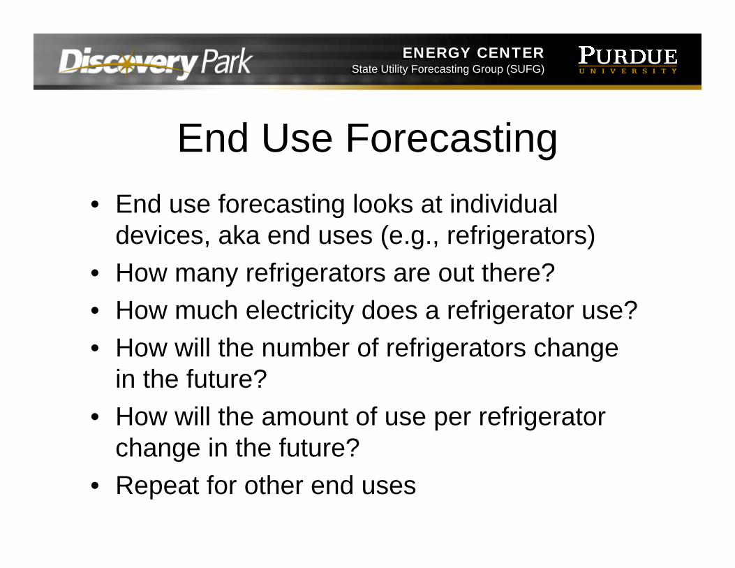
End Use Forecasting• End use forecasting looks at individual

devices, aka end uses (e.g., refrigerators)• How many refrigerators are out there?• How much electricity does a refrigerator use?• How will the number of refrigerators change

in the future?• How will the amount of use per refrigerator

change in the future?• Repeat for other end uses



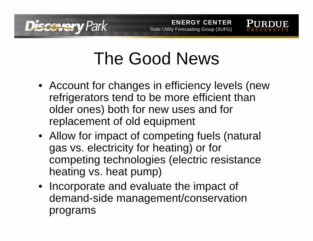
The Good News• Account for changes in efficiency levels (new

refrigerators tend to be more efficient than older ones) both for new uses and for replacement of old equipment

• Allow for impact of competing fuels (natural gas vs. electricity for heating) or for competing technologies (electric resistance heating vs. heat pump)

• Incorporate and evaluate the impact of demand-side management/conservation programs



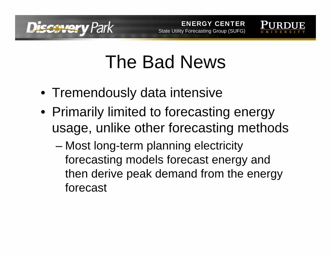
The Bad News• Tremendously data intensive• Primarily limited to forecasting energy

usage, unlike other forecasting methods– Most long-term planning electricity

forecasting models forecast energy and then derive peak demand from the energy forecast



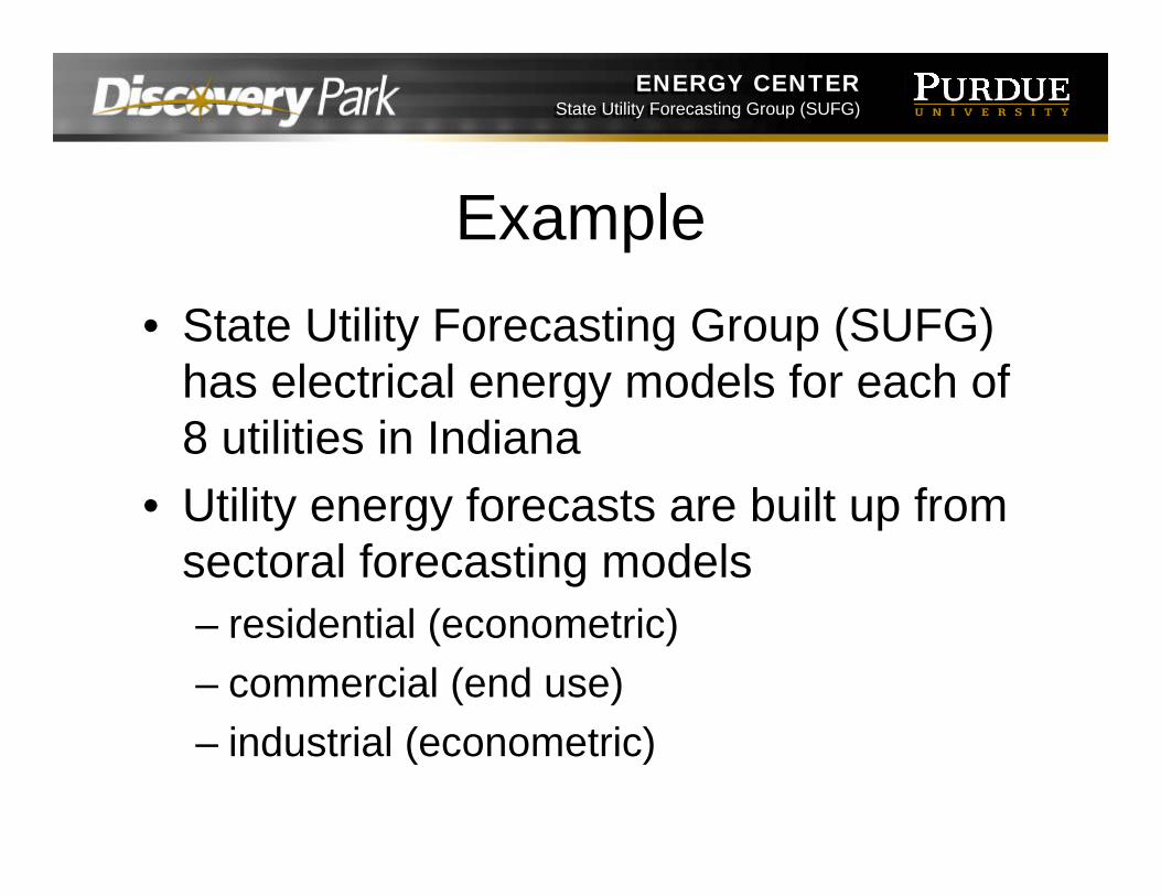
Example• State Utility Forecasting Group (SUFG)

has electrical energy models for each of 8 utilities in Indiana

• Utility energy forecasts are built up from sectoral forecasting models– residential (econometric)– commercial (end use)– industrial (econometric)



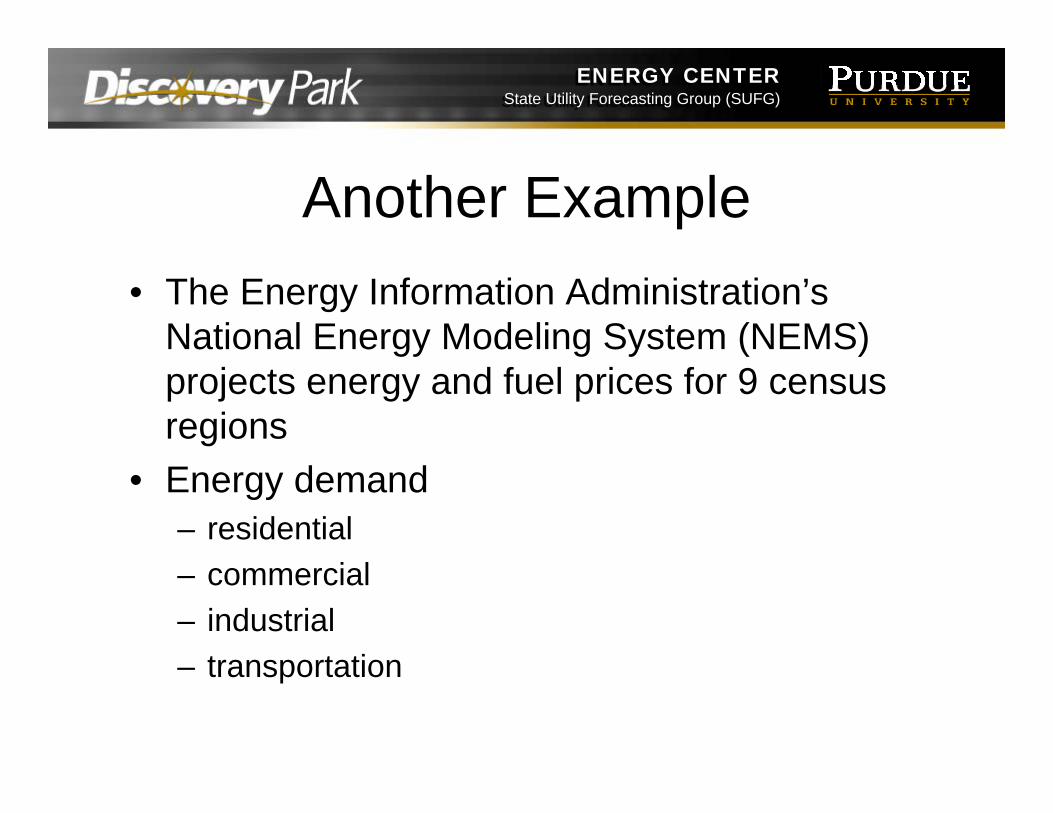
Another Example• The Energy Information Administration’s

National Energy Modeling System (NEMS) projects energy and fuel prices for 9 census regions

• Energy demand– residential– commercial– industrial– transportation



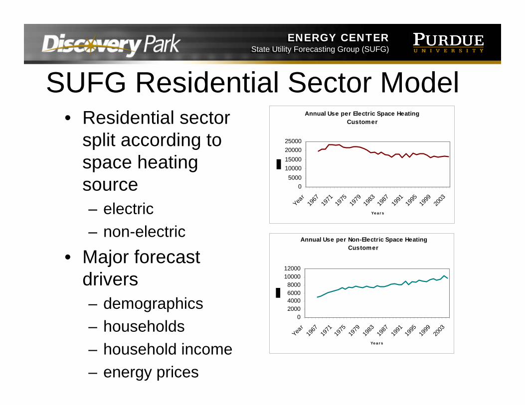
SUFG Residential Sector Model• Residential sector

split according to space heating source– electric– non-electric

• Major forecast drivers– demographics– households– household income– energy prices

Annual Use per Electric Space Heating Customer

05000

10000150002000025000

Year

1967

1971

1975

1979

1983

1987

1991

1995

1999

2003

Ye a r s

Annual Use per Non-Electric Space Heating Customer

02000400060008000

1000012000

Year

1967

1971

1975

1979

1983

1987

1991

1995

1999

2003

Ye a r s



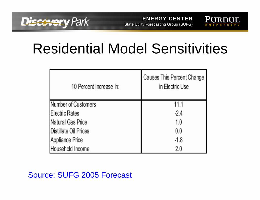
Residential Model Sensitivities

Source: SUFG 2005 Forecast



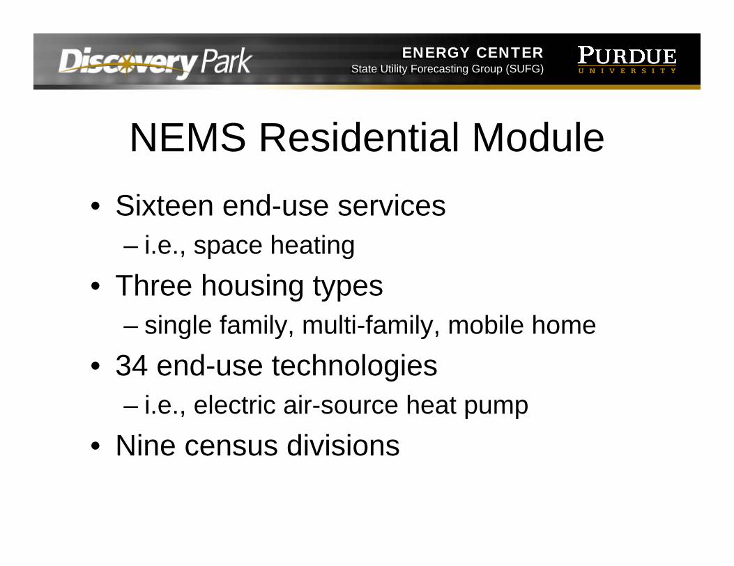
NEMS Residential Module• Sixteen end-use services

– i.e., space heating• Three housing types

– single family, multi-family, mobile home• 34 end-use technologies

– i.e., electric air-source heat pump• Nine census divisions



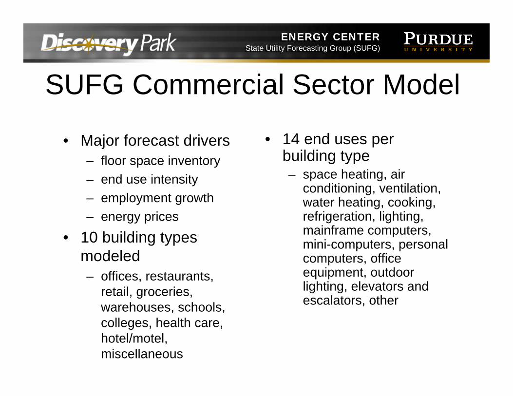
SUFG Commercial Sector Model

• Major forecast drivers– floor space inventory– end use intensity– employment growth– energy prices

• 10 building types modeled– offices, restaurants,

retail, groceries, warehouses, schools, colleges, health care, hotel/motel, miscellaneous

• 14 end uses per building type– space heating, air

conditioning, ventilation, water heating, cooking, refrigeration, lighting, mainframe computers, mini-computers, personal computers, office equipment, outdoor lighting, elevators and escalators, other



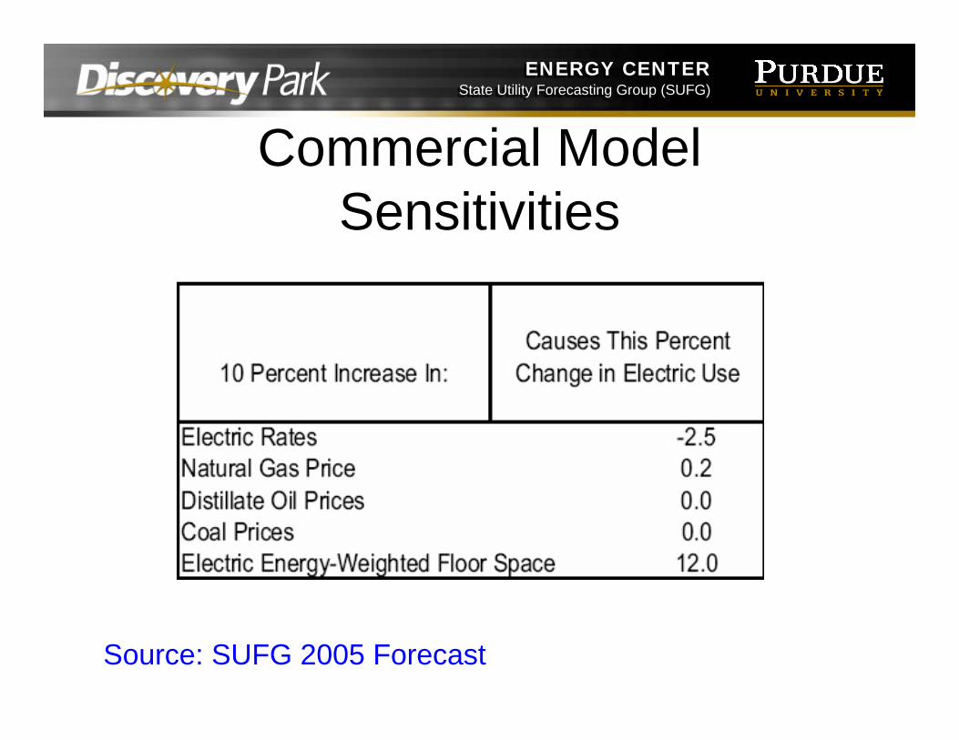
Commercial Model Sensitivities




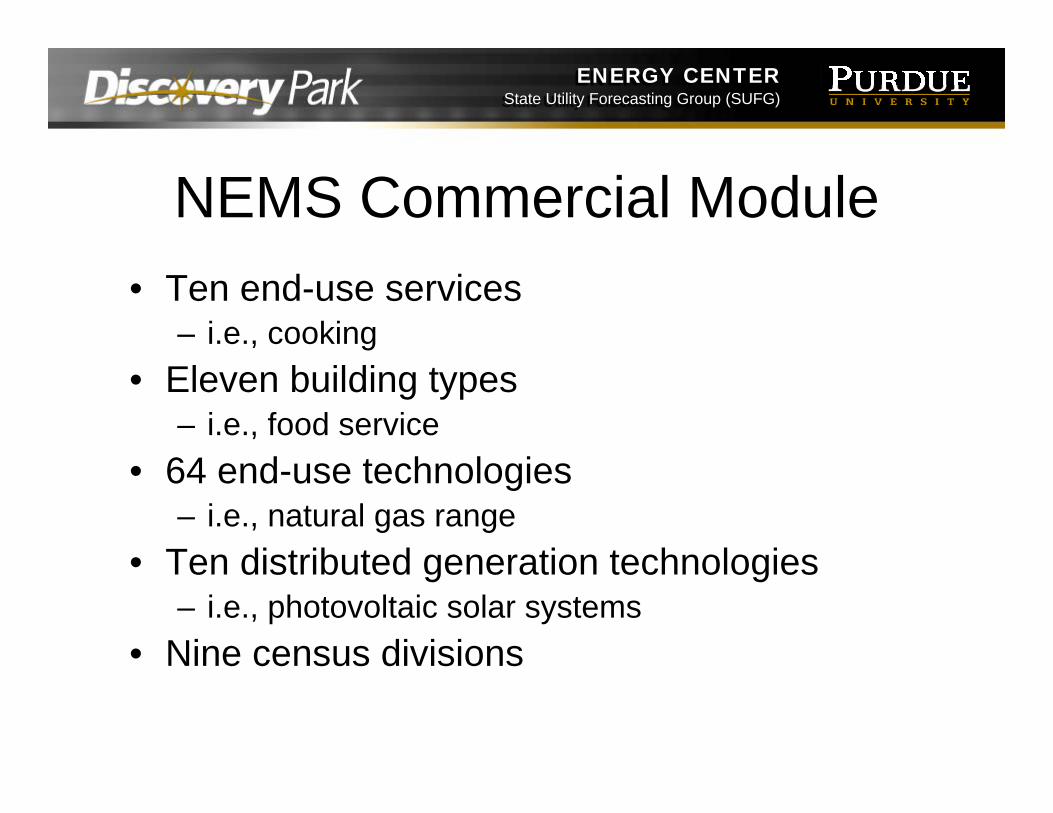
NEMS Commercial Module• Ten end-use services

– i.e., cooking• Eleven building types

– i.e., food service• 64 end-use technologies

– i.e., natural gas range• Ten distributed generation technologies

– i.e., photovoltaic solar systems• Nine census divisions



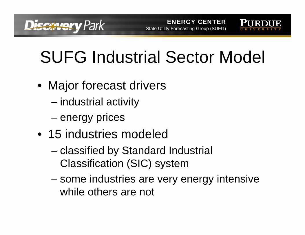
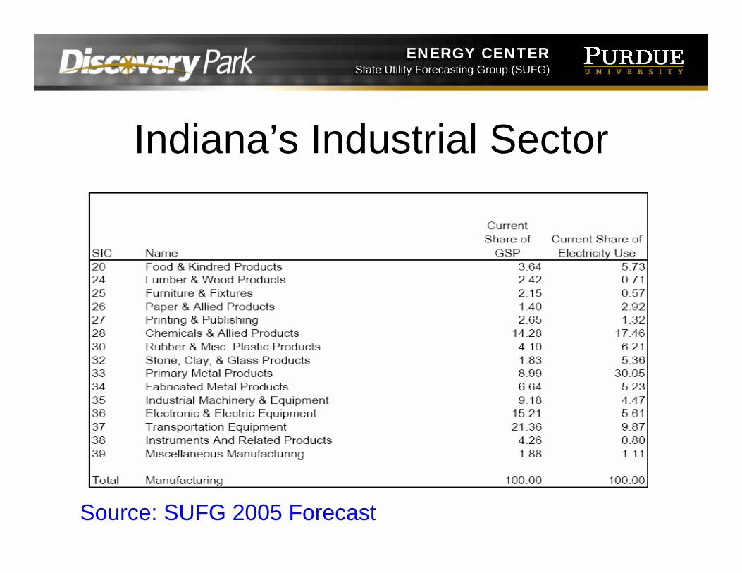
SUFG Industrial Sector Model• Major forecast drivers

– industrial activity– energy prices

• 15 industries modeled– classified by Standard Industrial

Classification (SIC) system– some industries are very energy intensive

while others are not



Indiana’s Industrial Sector




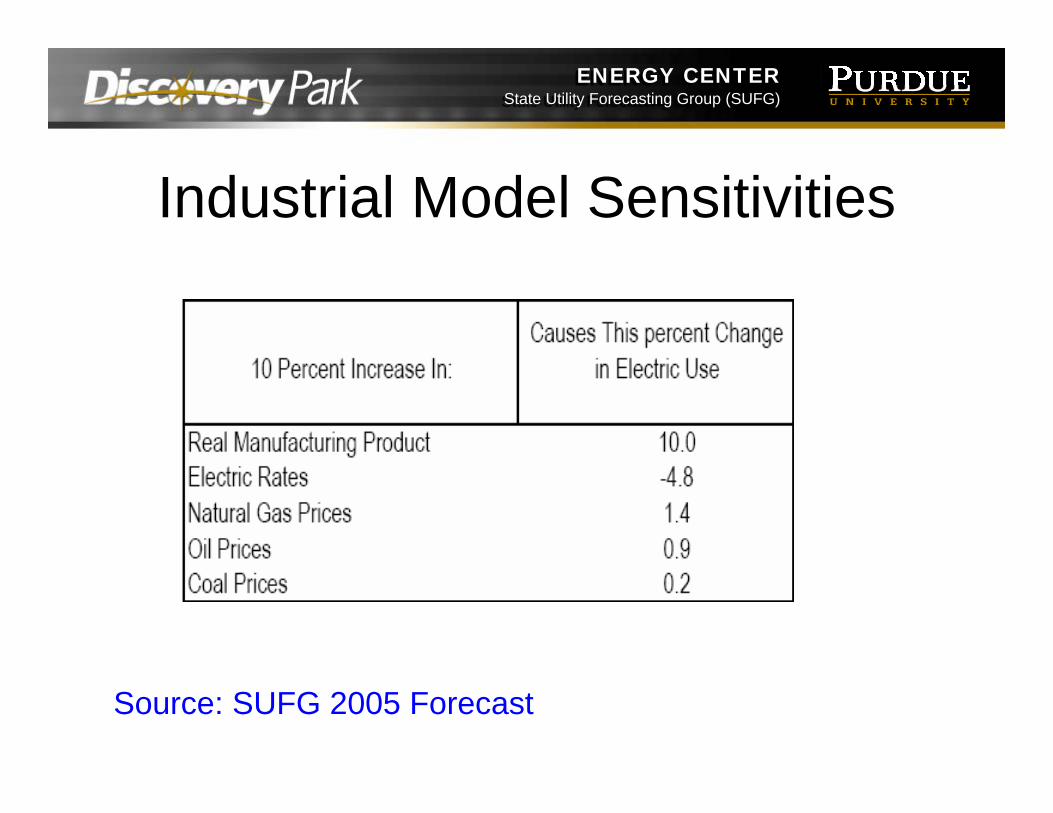
Industrial Model Sensitivities




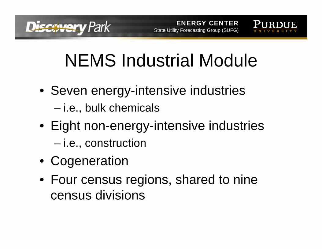
NEMS Industrial Module• Seven energy-intensive industries

– i.e., bulk chemicals• Eight non-energy-intensive industries

– i.e., construction• Cogeneration• Four census regions, shared to nine

census divisions



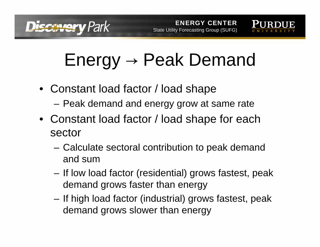
Energy → Peak Demand• Constant load factor / load shape

– Peak demand and energy grow at same rate• Constant load factor / load shape for each

sector– Calculate sectoral contribution to peak demand

and sum– If low load factor (residential) grows fastest, peak

demand grows faster than energy– If high load factor (industrial) grows fastest, peak

demand grows slower than energy



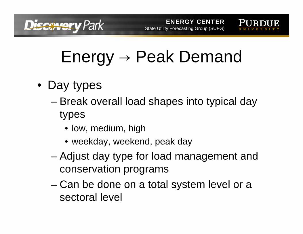
Energy → Peak Demand• Day types

– Break overall load shapes into typical day types

• low, medium, high• weekday, weekend, peak day

– Adjust day type for load management and conservation programs

– Can be done on a total system level or a sectoral level



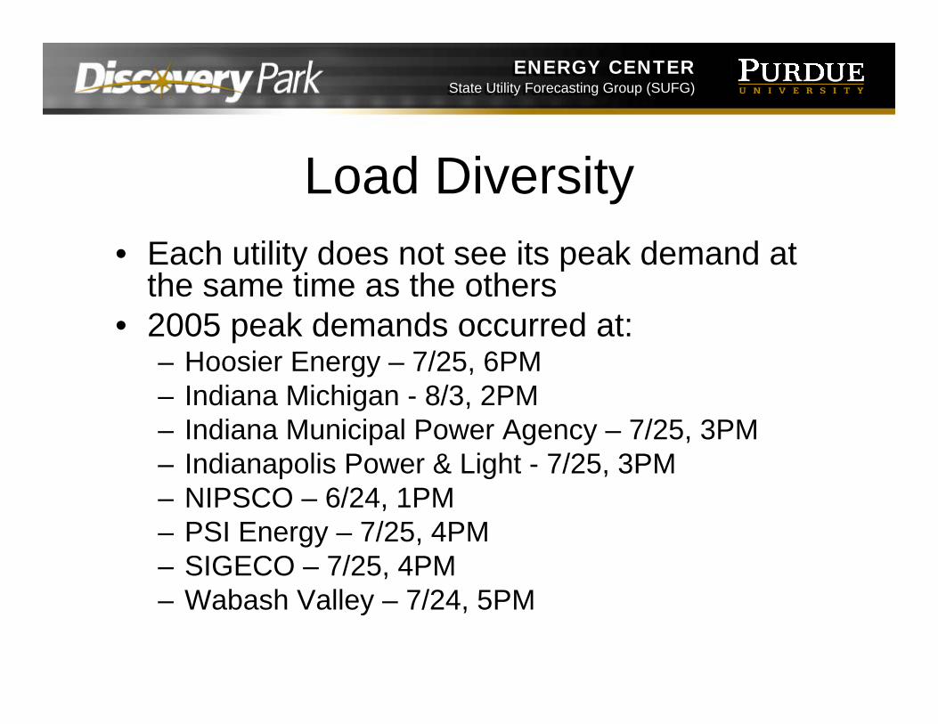
Load Diversity• Each utility does not see its peak demand at

the same time as the others• 2005 peak demands occurred at:

– Hoosier Energy – 7/25, 6PM– Indiana Michigan - 8/3, 2PM– Indiana Municipal Power Agency – 7/25, 3PM– Indianapolis Power & Light - 7/25, 3PM– NIPSCO – 6/24, 1PM– PSI Energy – 7/25, 4PM– SIGECO – 7/25, 4PM– Wabash Valley – 7/24, 5PM



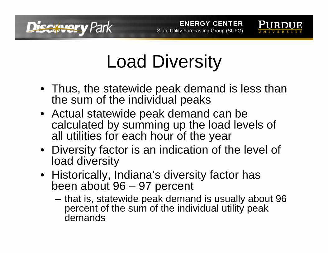
Load Diversity• Thus, the statewide peak demand is less than

the sum of the individual peaks• Actual statewide peak demand can be

calculated by summing up the load levels of all utilities for each hour of the year

• Diversity factor is an indication of the level of load diversity

• Historically, Indiana’s diversity factor has been about 96 – 97 percent– that is, statewide peak demand is usually about 96

percent of the sum of the individual utility peak demands



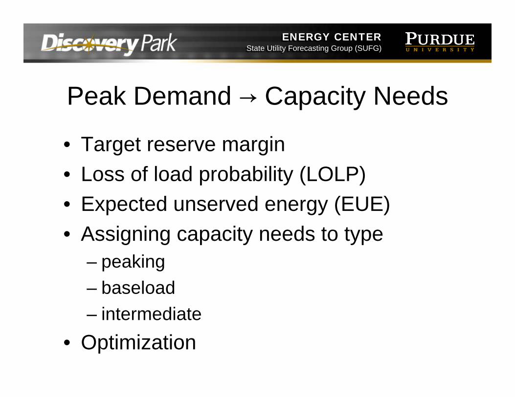
Peak Demand → Capacity Needs

• Target reserve margin• Loss of load probability (LOLP)• Expected unserved energy (EUE)• Assigning capacity needs to type

– peaking– baseload– intermediate

• Optimization



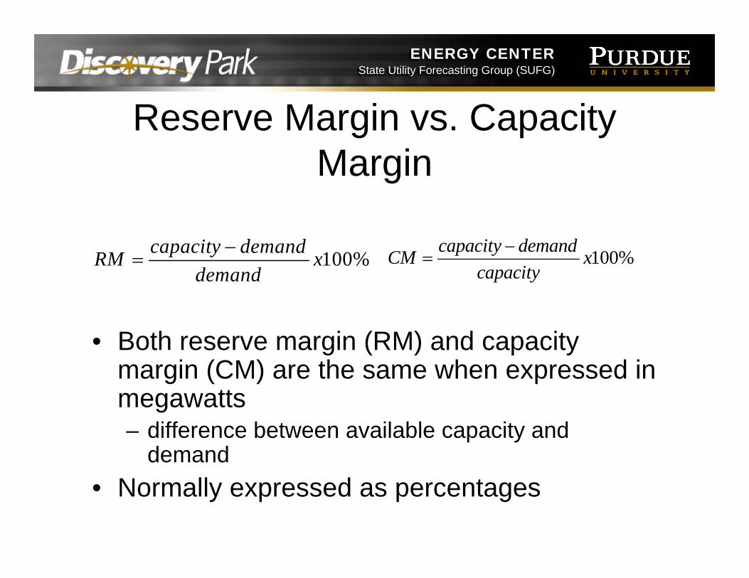
Reserve Margin vs. Capacity Margin

100%capacity demandCM xcapacity

−=

• Both reserve margin (RM) and capacity margin (CM) are the same when expressed in megawatts– difference between available capacity and

demand• Normally expressed as percentages

100%capacity demandRM xdemand

−=



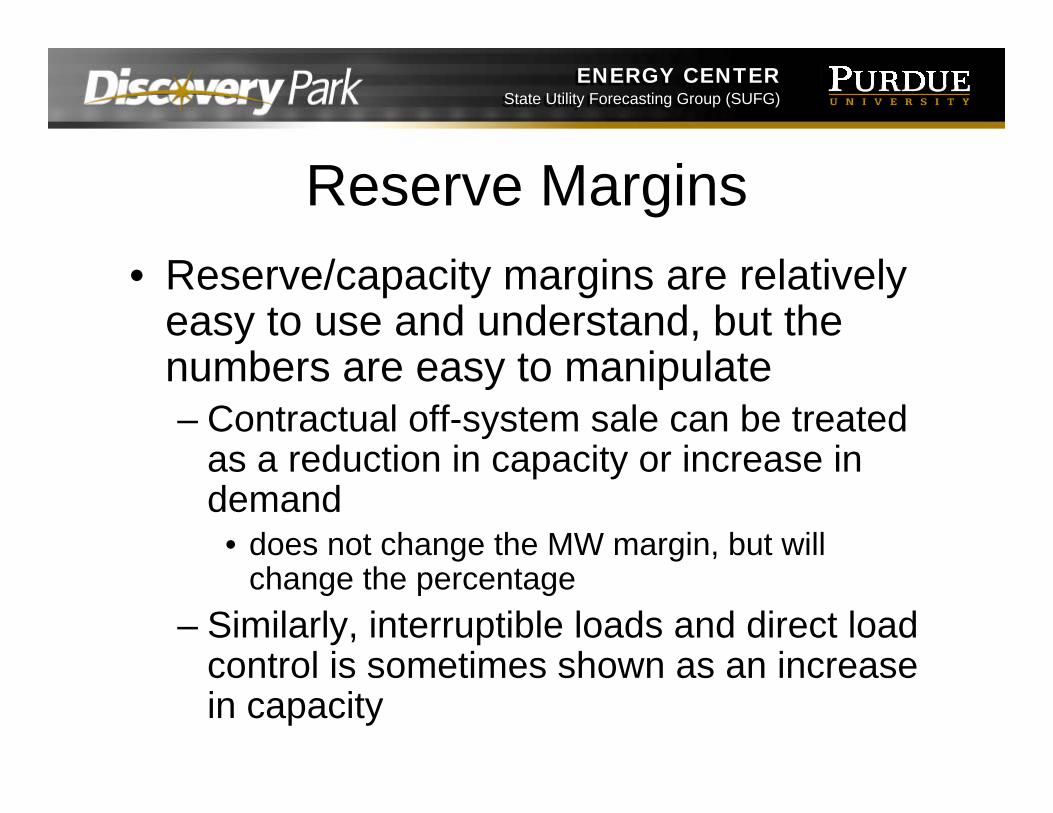
Reserve Margins• Reserve/capacity margins are relatively

easy to use and understand, but the numbers are easy to manipulate– Contractual off-system sale can be treated

as a reduction in capacity or increase in demand

• does not change the MW margin, but will change the percentage

– Similarly, interruptible loads and direct load control is sometimes shown as an increase in capacity



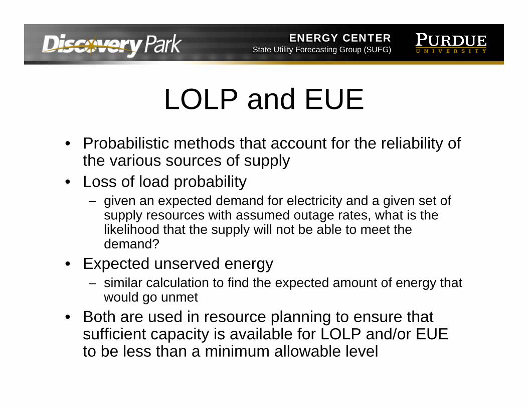
LOLP and EUE• Probabilistic methods that account for the reliability of

the various sources of supply• Loss of load probability

– given an expected demand for electricity and a given set of supply resources with assumed outage rates, what is the likelihood that the supply will not be able to meet the demand?

• Expected unserved energy– similar calculation to find the expected amount of energy that

would go unmet• Both are used in resource planning to ensure that

sufficient capacity is available for LOLP and/or EUE to be less than a minimum allowable level



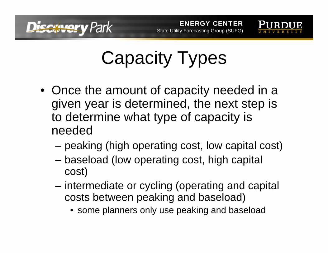
Capacity Types

• Once the amount of capacity needed in a given year is determined, the next step is to determine what type of capacity is needed– peaking (high operating cost, low capital cost)– baseload (low operating cost, high capital

cost)– intermediate or cycling (operating and capital

costs between peaking and baseload)• some planners only use peaking and baseload



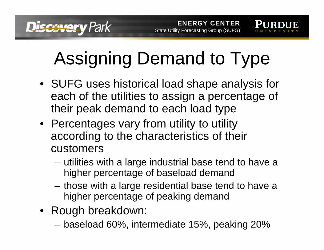
Assigning Demand to Type• SUFG uses historical load shape analysis for

each of the utilities to assign a percentage of their peak demand to each load type

• Percentages vary from utility to utility according to the characteristics of their customers– utilities with a large industrial base tend to have a

higher percentage of baseload demand– those with a large residential base tend to have a

higher percentage of peaking demand• Rough breakdown:

– baseload 60%, intermediate 15%, peaking 20%



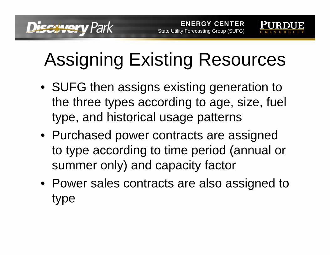
Assigning Existing Resources• SUFG then assigns existing generation to

the three types according to age, size, fuel type, and historical usage patterns

• Purchased power contracts are assigned to type according to time period (annual or summer only) and capacity factor

• Power sales contracts are also assigned to type



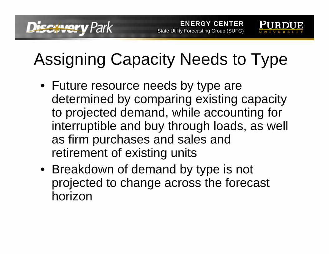
Assigning Capacity Needs to Type• Future resource needs by type are

determined by comparing existing capacity to projected demand, while accounting for interruptible and buy through loads, as well as firm purchases and sales and retirement of existing units

• Breakdown of demand by type is not projected to change across the forecast horizon



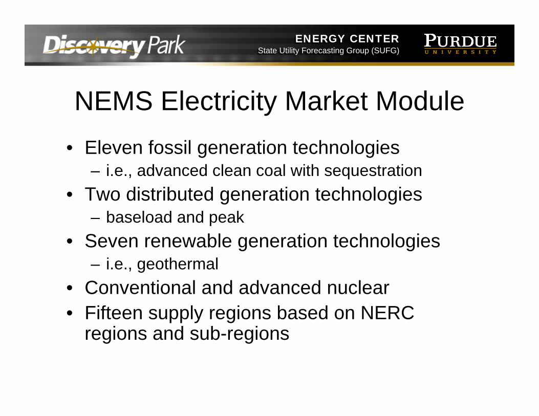
NEMS Electricity Market Module• Eleven fossil generation technologies

– i.e., advanced clean coal with sequestration• Two distributed generation technologies

– baseload and peak• Seven renewable generation technologies

– i.e., geothermal• Conventional and advanced nuclear• Fifteen supply regions based on NERC

regions and sub-regions



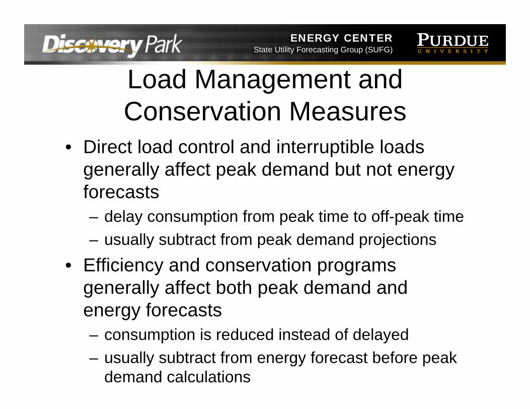
Load Management and Conservation Measures

• Direct load control and interruptible loads generally affect peak demand but not energy forecasts– delay consumption from peak time to off-peak time– usually subtract from peak demand projections

• Efficiency and conservation programs generally affect both peak demand and energy forecasts– consumption is reduced instead of delayed– usually subtract from energy forecast before peak

demand calculations



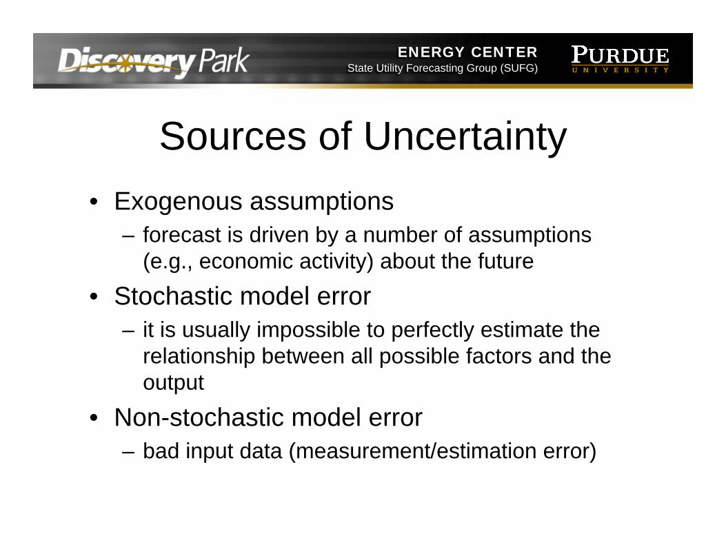
Sources of Uncertainty• Exogenous assumptions

– forecast is driven by a number of assumptions (e.g., economic activity) about the future

• Stochastic model error– it is usually impossible to perfectly estimate the

relationship between all possible factors and the output

• Non-stochastic model error– bad input data (measurement/estimation error)



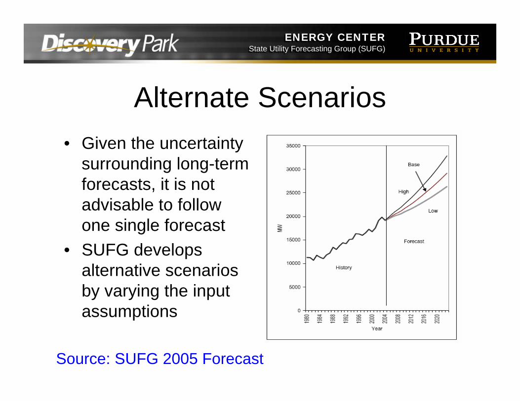
Alternate Scenarios• Given the uncertainty

surrounding long-term forecasts, it is not advisable to follow one single forecast

• SUFG develops alternative scenarios by varying the input assumptions




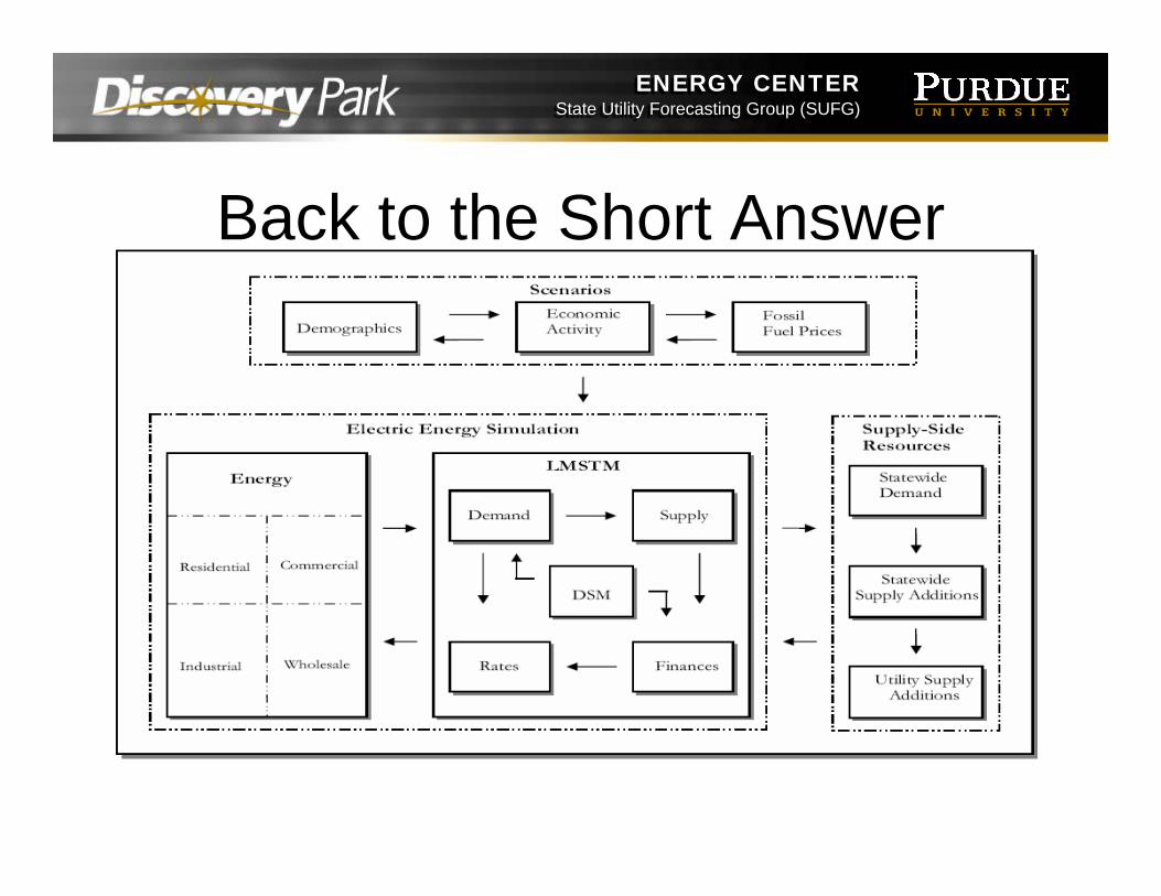
Back to the Short Answer



Further Information• State Utility Forecasting Group

– http://www.purdue.edu/dp/energy/SUFG/• Energy Information Administration

– http://www.eia.doe.gov/index.html

Energy Forecasting Methods - Purdue University -...

Documents

Transcript of Energy Forecasting Methods - Purdue University -...