ENERGY, ENVIRONMENT, BIOLOGY and BIOMEDICINE · ENERGY, ENVIRONMENT, BIOLOGY and BIOMEDICINE...

ENERGY, ENVIRONMENT, BIOLOGY and BIOMEDICINE

Proceedings of the 2014 International Conference on Energy, Environment, Ecosystems and Development II (EEED '14)

Proceedings of the 2014 International Conference on Biology and

Biomedicine II (BIO '14)

Prague, Czech Republic April 2‐4, 2014


Proceedings of the 2014 International Conference on Energy, Environment, Ecosystems and Development II (EEED '14) Proceedings of the 2014 International Conference on Biology and Biomedicine II (BIO '14)


Copyright © 2014, by the editors

All the copyright of the present book belongs to the editors. All rights reserved. No part of this publication may be reproduced, stored in a retrieval system, or transmitted in any form or by any means, electronic, mechanical, photocopying, recording, or otherwise, without the prior written permission of the editors.

All papers of the present volume were peer reviewed by no less than two independent reviewers. Acceptance was granted when both reviewers' recommendations were positive.

ISBN: 978‐1‐61804‐232‐3


Proceedings of the 2014 International Conference on Energy, Environment, Ecosystems and Development II (EEED '14)

Proceedings of the 2014 International Conference on Biology and

Biomedicine II (BIO '14)


Organizing Committee General Chairs (EDITORS)

Prof. Jan Awrejcewicz, Technical University of Lodz, Lodz, Poland

Prof. Marina Shitikova, Voronezh State University of Architecture and Civil Engineering, Voronezh, Russia

Prof. Vincenzo Niola University of Naples "Federico II" Via Claudio, 21 ‐ 80125 Naples ITALY

Prof. Thomas Panagopoulos, University of Algarve, Faro, Portugal

Prof. Wolfgang Wenzel, Institute for Nanotechnology, Germany

Prof. Florin Gorunescu, University of Medicine and Pharmacy of Craiova, Craiova, Romania

Prof. Ivana Horova, Masaryk University, Czech Republic

Prof. Andrei Korobeinikov, Centre de Recerca Matematica, Barcelona, Spain

Senior Program Chair

Prof. John Gordon Lindsay, (Professor of Medical Biochemistry) University of Glasgow, Glasgow, UK.

Prof. Seiji Shibasaki, Hyogo University of Health Sciences, Japan

Program Chairs

Prof. Bela Melegh, University of Pecs, Hungary

Prof. Gary A. Lorigan, Miami University, USA Idaho State University, USA

Prof. Ziad Fajloun, Universite Libanaise, Lebanon

Tutorials Chair

Prof. Nikolai N. Modyanov, University of Toledo, Toledo, USA

Special Session Chair

Prof. Dhavendra Kumar, University of South Wales, UK

Workshops Chair

Prof. Geoffrey Arden, European Vision Institute, UK

Local Organizing Chair

Assistant Prof. Klimis Ntalianis, Tech. Educ. Inst. of Athens (TEI), Athens, Greece

Publication Chair

Prof. Ferhan M. Atici, Department of Mathematics, Western Kentucky University, USA

Publicity Committee

Prof. Gerd Teschke, Institute for Computational Mathematics in Science and Technology, Neubrandenburg, Berlin‐Dahlem, Germany

Prof. Lucio Boccardo, Universita degli Studi di Roma "La Sapienza", Roma, Italy

International Liaisons Prof. Jia‐Jang Wu,

National Kaohsiung Marine University, Kaohsiung City, Taiwan

Prof. Giuseppe Carbone, University of Cassino and South Latium, Italy

Prof. Gilbert‐Rainer Gillich, "Eftimie Murgu" University of Resita, Romania

Prof. Yury A. Rossikhin, Voronezh State University of Architecture and Civil Engineering, Voronezh, Russia

Steering Committee Prof. Kim Choon Ng, National University of Singapore, Singapore Prof. Ravi P. Agarwal, Texas A&M University ‐ Kingsville, Kingsville, TX, USA Prof. Ahmet Selim Dalkilic, Yildiz Technical University, Besiktas, Istanbul, Turkey Prof. M. Affan Badar, Indiana State University, Terre Haute, Indiana, USA Prof. Dashan Fan, University of Wisconsin‐Milwaukee, Milwaukee, WI, USA Prof. Martin Bohner, Missouri University of Science and Technology, Rolla, Missouri, USA

Program Committee Prof. Bharat Doshi, John Hopkins University, Mayrland, USA Prof. Gang Yao, University of Illinois at Urbana ‐Champaign, USA Prof. Lu Peng, Luisian State University, Baton Rouge, LA, USA Prof. Y. Baudoin, Royal Military Academy, Brussels, Belgium Prof. Fotios Rigas, School of Chemical Engineering, National Technical University of Athens, Greece. Prof. S. Sohrab, Northwestern University, IL, USA Prof. A. Stamou, National Technical University of Athens, Greece Prof. A. I. Zouboulis, Dept. of Chemistry, Aristotle University of Thessaloniki, Greece. Prof. Z. A. Vale, ISEP ‐ Instituto Superior de Engenharia do Porto Rua Antonio Bernardino de Almeida, Portugal Prof. M. Heiermann, Dr., Department of Technology Assessment and Substance Flow, Potsdam, Germany Prof. I. Kazachkov, National Technical University of Ukraine (NTUU KPI ), Kyiv, Ukraine Prof. A. M.A. Kazim, UAE University, United Arab Emirates Prof. A. Kurbatskiy, Novosibirsk State University, Department of Physics, Russia Prof. S. Linderoth, Head of Research on Fuel Cells and Materials Chemistry at Riso National Laboratory. Denmark Prof. P. Lunghi, Dipartimento di Ingegneria Industriale, University degli Studi di Perugia, Italy Prof. J. Van Mierlo, Department of Electrotechnical Engineering and Energy Technology (ETEC) Vrije Universiteit Brussel, Belgium Prof. Pavel Loskot, Swansea University, UK Prof. N. Afgan, UNESCO Chair Holder, Instituto Superior Tecnico, Lisbon, Portugal Prof. F. Akgun, Gebze Kocaeli, Turkey Prof. Fernando Alvarez, Prof. of Economics, University of Chicago, USA Prof. Mark J. Perry, Prof. of Finance and Business Economics, University of Michigan‐Flit, USA Prof. Biswa Nath Datta, IEEE Fellow, Distinguished Research Professor, Northern Illinois University, USA Prof. Panos Pardalos, Distinguished Prof. Director, Center for Applied Optimization, University of Florida, USA Prof. Gamal Elnagar, University of South Carolina Upstate,Spartanburg, SC, USA Prof. Luis Tavares Rua, Cmte Guyubricht, 119. Conj. Jardim Costa do Sol. Atalaia, Brazil Prof. Igor Kuzle, Faculty of electrical engineering and computing, Zagreb, Croatia Prof. Maria do Rosario Alves Calado, University of Beira Interior, Portugal Prof. Gheorghe‐Daniel Andreescu, "Politehnica" University of Timisoara, Romania Prof. Jiri Strouhal, University of Economics Prague, Czech Republic Prof. Morris Adelman, Prof. of Economics, Emeritus, MIT, USA Prof. Germano Lambert‐Torres, Itajuba,MG, Brazil Prof. Jiri Klima, Technical faculty of CZU in Prague, Czech Republic Prof. Goricanec Darko, University of Maribor, Maribor, Slovenia Prof. Ze Santos, Rua A, 119. Conj. Jardim Costa do Sol, Brazil Prof. Ehab Bayoumi, Chalmers University of Technology,Goteborg, Sweden Prof. Robert L. Bishop, Prof. of Economics, Emeritus, MIT, USA Prof. Glenn Loury, Prof. of Economics, Brown University, USA Prof. Patricia Jota, Av. Amazonas 7675, BH, MG, Brazil Prof. S. Ozdogan, Marmara University, Goztepe Campus, Kuyubasi, Kadikoy, Istanbul, Turkey

Additional Reviewers Lesley Farmer California State University Long Beach, CA, USA

Kei Eguchi Fukuoka Institute of Technology, Japan

James Vance The University of Virginia's College at Wise, VA, USA

Eleazar Jimenez Serrano Kyushu University, Japan

Zhong‐Jie Han Tianjin University, China

Minhui Yan Shanghai Maritime University, China

George Barreto Pontificia Universidad Javeriana, Colombia

Tetsuya Shimamura Saitama University, Japan

Shinji Osada Gifu University School of Medicine, Japan

Genqi Xu Tianjin University, China

Jose Flores The University of South Dakota, SD, USA

Philippe Dondon Institut polytechnique de Bordeaux, France

Imre Rudas Obuda University, Budapest, Hungary

Abelha Antonio Universidade do Minho, Portugal

Tetsuya Yoshida Hokkaido University, Japan

Sorinel Oprisan College of Charleston, CA, USA

Xiang Bai Huazhong University of Science and Technology, China

Francesco Rotondo Polytechnic of Bari University, Italy

Valeri Mladenov Technical University of Sofia, Bulgaria

Stavros Ponis National Technical University of Athens, Greece

Matthias Buyle Artesis Hogeschool Antwerpen, Belgium

José Carlos Metrôlho Instituto Politecnico de Castelo Branco, Portugal

Kazuhiko Natori Toho University, Japan

Ole Christian Boe Norwegian Military Academy, Norway

Alejandro Fuentes‐Penna Universidad Autónoma del Estado de Hidalgo, Mexico

João Bastos Instituto Superior de Engenharia do Porto, Portugal

Masaji Tanaka Okayama University of Science, Japan

Yamagishi Hiromitsu Ehime University, Japan

Manoj K. Jha Morgan State University in Baltimore, USA

Frederic Kuznik National Institute of Applied Sciences, Lyon, France

Dmitrijs Serdjuks Riga Technical University, Latvia

Andrey Dmitriev Russian Academy of Sciences, Russia

Francesco Zirilli Sapienza Universita di Roma, Italy

Hessam Ghasemnejad Kingston University London, UK

Bazil Taha Ahmed Universidad Autonoma de Madrid, Spain

Jon Burley Michigan State University, MI, USA

Takuya Yamano Kanagawa University, Japan

Miguel Carriegos Universidad de Leon, Spain

Deolinda Rasteiro Coimbra Institute of Engineering, Portugal

Santoso Wibowo CQ University, Australia

M. Javed Khan Tuskegee University, AL, USA

Konstantin Volkov Kingston University London, UK

Moran Wang Tsinghua University, China

Angel F. Tenorio Universidad Pablo de Olavide, Spain

Table of Contents

Keynote Lecture 1: Interpolation and Projective Representation in Computer Graphics, Visualization and Games

11

Vaclav Skala, Rongjiang Pan

Gravity Control: Modeling and Experiments 13

Vitaly O. Groppen

Numerical Investigation of Diffusion Turbulent Propane/Air Flame 18

S. Morsli, M. El Ganaoui, A. Sabeur‐Bendehina

Indicator Based Sustainability Analysis of Future Energy Situation of Santiago de Chile 24

Volker Stelzer, Adriana Quintero, Luis Vargas, Gonzalo Paredes, Sonja Simon, Kristina Nienhaus, Jürgen Kopfmüller

A Scalable Method for Efficient Stem Cell Donor HLA Genotype Match Determination 28

D. Georgiev, L. Houdová, M. Fetter, P. Jindra

Denoising of Noisy MRI Brain Image by Using Switching‐Based Clustering Algorithm 33

Siti Noraini Sulaiman, Siti Mastura Che Ishak, Iza Sazanita Isa, Norhazimi Hamzah

Energy Efficiency of Conservative Tillage Systems in the Hilly Areas of Romania 40

Rusu Teodor

A Suggested Method for Assessing Cliff Instability Susceptibility at a Given Scale (CISA) 45

G. F. Andriani, V. Pellegrini

Sex‐Specific Effect of the LDL‐Receptor rs6511720 Polymorphism on Plasma Cholesterol Levels. Results from the Czech post‐MONICA Study

51

Jaroslav A. Hubacek, Vera Lanska, Vera Adamkova

Segmentation of Brain MRI Image Based on Clustering Algorithm 54

Siti Noraini Sulaiman, Noreliani Awang Non, Iza Sazanita Isa, Norhazimi Hamzah

Effects of Adolescent Idiopathic Scoliosis on Postural Balance and Muscle Activity 60

J. Y. Jung, C. I. Yoo, I. S. Park, Y. G. Won, B. O. Kim, S. K. Bok, J. J. Kim

The Double Reflection Control of Direct Solar Light in Deep Atrium Type Spaces 65

Ioan Borza, Claudiu Silvasan

Possible Assessment on Sustainability of Slopes by Using Electrical Resistivity: Comparison of Field and Laboratory Results

69

Syed B. Syed Osman, Fahad I. Siddiqui

Energy, Environment, Biology and Biomedicine

ISBN: 978-1-61804-232-3 9

Simple and Routinely Affordable Method for Therapeutic Monitoring of Levetiracetam: A Comparison to Often Applied HPLC Method

74

Tesfaye H., Skokanova J., Jedličkova B., Prusa R., Kotaska K., Sebronova V., Elisak M.

New Tree Species for Agroforestry and Energy Purposes 82

Andrea Vityi, Béla Marosvölgyi

Extremely Delayed Elimination of Methotrexate in a Young Man with Osteosarcoma: A Case Study Demonstrating an Association with Impaired Renal Function

85

Tesfaye H., Beyerova M., Jedlickova B., Korandova A., Linke Z., Becvarova M., Shimota M.

Transmission Corridor between Romania‐Moldova‐Ukraine 91

Udrea Oana, Gheorghe Lazaroiu

Bimarkers and Their Utlization in Clinical Medicine: A Contribution to the State of the Art 99

Tesfaye H.

Authors Index 111


ISBN: 978-1-61804-232-3 10

Keynote Lecture 1

Interpolation and Projective Representation in Computer Graphics, Visualization and Games

Vaclav Skala University of West Bohemia

Plzen, Czech Republic E‐mail: [email protected]

Rongjiang Pan Shandong University

Jinan, China E‐mail: [email protected]

Abstract: Today's engineering problem solutions are based mostly on computational packages. However the computational power doubles in 18 months. In 15 years perspective the computational power will be of 2^10 = 1024 of today's computational power. Engineering problems solved will be more complicated, complex and will lead to a numerically ill conditioned problems especially in the perspective of today available floating point representation and formulation in the Euclidean space. Homogeneous coordinates and projective geometry are mostly connected with geometric transformations only. However the projective extension of the Euclidean system allows reformulation of geometrical problems which can be easily solved. In many cases quite complicated formulae are becoming simple from the geometrical and computational point of view. In addition they lead to simple parallelization and to matrix‐vector operations which are convenient for matrix‐vector hardware architecture like GPU. In this short tutorial we will introduce "practical theory" of the projective space and homogeneous coordinates. We will show that a solution of linear system of equations is equivalent to generalized cross product and how this influences basic geometrical algorithms. The projective formulation is also convenient for computation of barycentric coordinates, as it is actually one cross‐product implemented as one clock instruction on GPU. Selected examples of engineering disasters caused by non‐robust computations will be presented as well. Brief Biography of the Speaker: Prof.Vaclav Skala is a Full professor of Computer Science at the University of West Bohemia, Plzen, Czech Republic. He received his Ing. (equivalent of MSc.) degree in 1975 from the Institute of Technology in Plzen and CSc. (equivalent of Ph.D.) degree from the Czech Technical University in Prague in 1981. In 1996 he became a full professor in Computer Science. He is the Head of the Center of Computer Graphics and Visualization at the University of West Bohemia in Plzen (http://Graphics.zcu.cz) since 1996. Prof.Vaclav Skala is a member of editorial board of The Visual Computer (Springer), Computers and Graphics (Elsevier), Machine Graphics and Vision (Polish Academy of Sciences), The International Journal of Virtual Reality (IPI Press, USA) and the Editor in Chief of the Journal of WSCG. He has been a member of several international program committees of prestigious conferences and workshops. He is a member of ACM SIGGRAPH, IEEE and Eurographics Association. He became a Fellow of the Eurographics Association in 2010.


ISBN: 978-1-61804-232-3 11

Prof.Vaclav Skala has published over 200 research papers in scientific journal and at international research conferences. His current research interests are computer graphics, visualization and mathematics, especially geometrical algebra, algorithms and data structures. Details can be found at http://www.VaclavSkala.eu Prof. Rongjiang Pan is a professor in the School of Computer Science and Technology, Shandong University, China. He received a BSc in computer science, a Msc in computer science, a PhD in computer science from Shandong University, China in 1996, 2001 and 2005, respectively. During 2006 and 2007, he was a visiting scholar at the University of West Bohemia in Plzen under a program supported by the international exchange scholarship between China and Czech governments. He is now a visiting professor at the School of Engineering, Brown University from 2014 to 2105 under the support of China Scholarship Council. He is a Member of the ACM. His research interests include 3D shape modeling and analysis, computer graphics and vision, image processing. He has published over 20 research papers in journal and at conferences


ISBN: 978-1-61804-232-3 12

Gravity control: modeling and experiments

Vitaly O. Groppen

Abstract—Paper describes statement and results of

experiments which are based on the use of high voltage for

verification of gravity control possibility. Used verification technology is based on the idea of substitution of energy

distributed in the neighborhood above the upper surface of the

plate-deployed capacitor by the material point with equivalent

mass: force of the gravitational interaction of the plate with this point has opposite direction to the force of gravitational

interaction of this plate with the Earth thus reducing this force.

Results of experiments with different samples confirm the

correctness of the proposed approach.

Keywords— Experimental verification, gravity control, high

voltage, samples, weight measurement.

I. Introduction

The equation published in England by Sir Isaac Newton in

1667 [1] can be considered as the first attempt to describe

the forces of gravity. About 250 years later, in 1915, in [2]

Albert Einstein demonstrated a new theory of gravitation

based on the Theory of Relativity. Movement of physical

objects under the influence of high voltage discovered by

Townsend Brown in 1921 cannot be considered as control

of gravitational forces because this phenomenon is known

to be caused by ionization of air atoms near acute and sharp

edges [3]. The experiments outlined below are also based

on the use of high voltage for verification of gravity control

possibility. They are based on the idea of substitution of

energy distributed in the neighborhood above the upper

surface of the plate-deployed capacitor by the material

point with equivalent mass: force of the gravitational

interaction of the plate with this point is directed opposite

to the direction of the force of gravitational interaction of

this plate with the Earth therefore reducing the plate’s

weight.

II. Main Principles

Electrodes of used in experiments plates are designed as metal

strips of deployed capacitors so that their stored energy is

distributed above the upper surface of a horizontally

positioned plate (see Fig. 2a and Fig. 3a below). This energy

Ei of i-th plate is equal to:

This work is supported by Grant of the Ministry of Education and Science of

the Russian Federation. V.O. Groppen is with the North-Caucasian Institute of

Mining and Metallurgy (State Technological University), Data Processing

Department; North Ossetia, 362021 Vladikavkaz, Russia;

phone: +79054899900; fax +78672407203; e-mail: [email protected]

(1) ,2

:2

UCEi i

i

where “Ci” is capacity of a charged plate-capacitor, “U” -

power supply voltage.

The mass of this energy is determined as follows:

(2) ,2

)(:2

2

c

UCEmi i

i

where “c” - velocity of light.

Below we use the model, in which:

a) the plates are disposed horizontally, so that the electrodes

are on their upper surface;

b) distributed above the upper surface of the i-th plate

energy is replaced by the equivalent body D, whose mass is

determined by the expression (2).

Thus the force Fi of the gravitational interaction between the i-

th plate and body D has a direction opposite to the force Fe of

gravitational interaction between this plate and the Earth (Fig.

1).

Fig.1. The forces of interaction between the body D, i-th plate

and Earth.

Force Fi value in accordance with (2), is determined by the low

of gravity:

(3) ,2

:22

2

cR

UCmFi ii

i

where “γ” - gravitational constant, “R” - distance between the

body D and the surface of the i-th plate (Fig. 1).

Denoting 0

eF the weight of a plate before experiment whereas

1

eF - its weight during experiment when the electrodes on its

surface are applied to voltage equal to U, it is easy to determine

value Fi: . :10

eei FFFi (4)

Fixing, for each plate in the experiments according to (4) all

components of the equation (3) except distance R, the latter for

i-th plate can be defined as:

R Fi

Fe

D

i-th plate

Surface of the Earth


ISBN: 978-1-61804-232-3 13

(5) .2

)( ,i

ii

iF

Cm

c

UURi

In a first approximation, the experimentally obtained values of

Ri (U) can be set by a polynomial:

(6) ,)(:2

0

,

jj

j

jii UkURi

where “ki,j “– j-th coefficient in equation (6) for i-th plate.

Substituting (6) into equation (3) it is possible to predict Fi

values outside the range of voltages U, fixed during the

experiments, using the expression:

(7) ,

2

:

2

22

0

,

2

cUk

UCmFi

jj

j

ji

iii

Using (7) it can be shown that the lifting force Fi, which is

equal to the weight of the i-th plate, corresponds to the voltage

U, being solution of the following square equation:

(8) .2

:

2

0

,g

C

c

UUki ij

j

j

ji

III. Equipment, experiments statement and

samples for gravity control

To verify the assumptions above during the first series of

experiments (see [4], [5]) we used different light and thin fiber

glass with lavsan cover plates with two groups of cooper

electrodes on the upper side of each plate (Fig. 2a) connected

to the high voltage power supply IVNR-20/10 (guarantying

voltage range 1 – 20 kV, power 200 wt., see Fig. 2b,1) and

installed on the weight table of precise electronic scale AV-

60/01-S (precision is equal to 0.0001 g, maximum weight – 60

g., the settling time of weighting mode – about 10 minutes, Fig.

2b,2).

a b

Fig. 2. Geometry of electrodes on the upper surface of the

plates (a) and equipment (b) used in the first series of gravity

control experiments.

Detailed descriptions of scheme and results of these

experiments is provided in [5], there seems to be three typical

sources of weight value mistakes during these series of

experiments:

experiments for direct weight measurement of

samples under high voltage resulted in direct

interaction of electronic circuit of the scale and its

sensor with the electric field on the upper surface of a

sample often resulting in distortions in indications of

weight by the scale (Fig. 2b, 3) and even in blocking

of electronics of the scale;

aspiration to increase the energy stored by sample-

capacitor increasing its capacity by reducing the

distance between the electrodes, resulted in downturn

of breakdown voltage, which ultimately contributed to

the opposite effect - a decrease of stored energy;

as shown in [5], any prolonged exposure of different

samples based on fibre glass with lavsan cover to high

voltage leads to its’ electrical breakdown, thus

eliminating possibility of a repetition of the

experiment.

To minimize the errors indicated above, during the

second series of experiments we used:

new samples with better resistance to electrical

breakdown made of granite with two spaced apart

parallel copper strips, attached to the top of each

granite rectangle (see below Fig. 3a and Table 1);

new precision balance AB-200 with maximum weight

equal to 200 gram and precision equal to 0.001 g (Fig

3b), which is not exposed to electromagnetic

radiation;

new scheme of experiments making use of all the

possibilities of the new equipment.

a b

Fig. 3. The copper electrodes on the upper

surface of the granite plates (a) and mechanical

scale AB-200 (b) used in the second series of

experiments.

To improve the accuracy of weighing along with the standard

metal weights were used narrow strips of paper. The scheme of

experiments for each sample was determined by the following

algorithm.

2

1

3

a

b

c


ISBN: 978-1-61804-232-3 14

Table 1. Parameters of the samples used during the

second series of experiments.

Algorithm

Step 1. A sample is installed on the left weighing

pan of precision mechanical scale AB-200 and

balanced.

Step 2. A new, previously unused voltage is

selected by the power supply IVNR-20/10 and

applied to the sample.

Step 3. As during the previous step scale was

unbalanced, we restore balance by removing part of

the weights from the right weighing pan.

Step 4. The high voltage source is turned off.

Step 5. The weights tucked away on the third step

of the current iteration are weighed by precision

electronic scales AV-60/01-S. The total weight of

these weights is shown by the scale display.

Step 6. We fix voltage, selected on the second step

of the current iteration and corresponding change of

weight of used sample.

Step 7. If experiments are carried out with all the

planned values of high voltage, then go to step 8,

otherwise mechanical scales AB-200 are balanced

again and we go to the second step.

Step 8. The series of experiments with the sample

selected at the first step is completed.

IV. Results of experiments

Voltage and corresponding change of weight for each sample

are presented in the appendix whereas equation (6) coefficients

for each sample described in the Table 3 are presented below

(distance Ri , i ϵ {a, b, c}, is given in meters, voltage U – in

volts):

Ra(U) = - 2.998478∙10-14

+ 7.847125∙10-18

∙U

- 3.021905∙10-22

∙U2; (9)

13 kV ≤ U ≤ 16 kV.

Rb(U) = 1.034423∙10-14

- 4.466534∙10-19

∙U

+ 1.060829∙10-23

∙U2; (10)

9 kV ≤ U ≤ 20 kV.

Rс(U) = 1.554385∙10-15

- 1.094039∙10-19

∙U

+ 3.561179∙10-23

∙U2; (11)

2.5 kV ≤ U ≤ 15 kV.

In the equations (9) and (10), the relative error does not exceed

five percent, with the voltage changes in the range of 9 – 20

kV, whereas in equation (11) the relative error does not exceed

29 percent if the voltage changes in the range of 2.5 - 15 kV.

The relative deviation of the calculated lifting force obtained

through the equation (9) or (10) substitution into equation (7)

from its experimental value does not exceed ten percent

whereas the upper bound of the relative deviation of the

calculated lifting force resulting equation (11) substitution into

equation (7) is equal to the 46%.

Substitution of (9) into (8) for voltage U value

determination in the case when the lifting force Fa value is

equal to the weight of the sample “a” in Fig. 3a, results in the

values equal to either 1990.744 V or to 49843.05 V. Similar

substitution of (10) into equation (8) for voltage U value

determination for the case when the lifting force Fb value is

equal to the weight of the sample “b” in Fig. 3a, results in the

values equal to either 13396.5 V or to 72788.28 V. The control

series of experiments with the lower values of voltage applied

to the both samples did not result in the corresponding lifting

forces. The efforts to predict constant voltage U value resulting

in lifting force equal to the weight of sample “c” in Fig. 3a, by

substitution of (11) into equation (8) failed: the resulting

№ Parameter

name

Labels of samples in Fig. 3a Measure-

ment

units

a b с

1 2 3 4 5 6

1 Upper

surface

area

0.0063 0.003072 0.0016 m2.

2 Total

surface

area

0.0158 0.008704 0.0048 m2.

3 Weight 211.0 85.16 55.07 gm.

4 Thickness 10.0 10.0 10.0 mm.

5 Distance

between

the electrodes

30.0 22.0 26.0 mm.

6 Width of

the

electrodes

11.0 5.0 7.0 mm.

7 Capacity 6.166 2.9 1.6 pF

8 Material

of the

plate basis

Granite

-


ISBN: 978-1-61804-232-3 15

voltage is a complex value containing real and imaginary

components.

V. Conclusions

The above presented approach allows us to make the following

conclusions:

1. Results of experiments convince of the correctness

of the proposed idea of gravity control.

2. As the lower values of voltage applied to the

samples “a” and “b” during the experiments did

not result in the corresponding lifting forces and

the efforts to predict constant voltage U value

resulting in lifting force equal to the weight of

sample “c” using dependence distance / voltage

defined by equation (6) failed, further experiments

will be focused on:

a wider range of voltages, overlapping defined

above upper voltage values;

the search of dependence distance / voltage

different from the model defined by equation (6).

Appendix

The tables below contain the results of experiments

with the samples "a", "b" and "c" whose parameters are

given above in Table 1. The first column of each table

contains the number of experiment of the current series

of experiments, the second column - the voltage applied

to the sample, and the third - the proper lifting force.

Table 2. Voltage and corresponding change of

lifting force Fa for the sample “a” (Fig. 3a)

# U (V) Fa (kg)

1 0 0

2 13000 0.0000187

3 14000 0.0000231

4 14500 0.0000268

5 15000 0.0000265

6 15500 0.000032

7 16000 0.0000393

Table 3. Voltage and corresponding change

of lifting force Fb for the sample “b” (Fig. 3a)

# U (V) Fb (kg)

1 0 0

2 9000 0.0000144

3 10000 0.0000194

4 11000 0.0000281

5 12000 0.000029

6 13000 0.0000376

7 14000 0.0000524

8 15000 0.0000540

9 16000 0.0000755

10 17000 0.0000773

11 18000 0.0000865

12 19000 0.0001108

13 20000 0.0001156

Table 4.Voltage and corresponding change of

lifting force Fc for the sample “c” (Fig. 3a).

Acknowledgment

I’m pleased to thank Ann Minevitch for assistance in preparing

of English version of this work.

References

[1] I. Newton. The mathematical principles of

natural knowledge, 1667.

[2] A. Einstein. The theory of relativity. Die Physik,

Under reduction of E. Lechner, Leipzig, V. 3,

1915, pp. 703 – 713, (in German).

# U (V) Fc (kg)

1 2500 0.0000116

2 3000 0.000013

3 4000 0.0000223

4 5000 0.0000158

5 7500 0.0000248

6 10000 0.0000182

7 14000 0.0000221

8 15000 0.000009


ISBN: 978-1-61804-232-3 16

[3] D.R. Buehler. Exploratory Research on the

Phenomenon of the Movement of High Voltage

Capacitors, Journal of Space Mixing, April

2004, vol. 2, pp. 1-22.

[4] V.O. Groppen, Spontaneous Mass Loss as a

Tool of Gravity Control. Recent Advances in

Systems Science & Mathematical Modeling, in

Proc. of the 3-rd Int. Conf. on Mathematical

Models for Engineering Science (MMES’12).

Paris, France, December 2 – 4, 2012, pp. 85 –

89.

[5] V.O. Groppen . Manifestations of Measurement

Standards Variability in the Universe Modeling,

Lambert Academic Publishing, Saarbrucken,

Germany, 2013, 76p.


ISBN: 978-1-61804-232-3 17

http://www.space-mixing-theory.com/abstract2.htm



Abstract— The turbulent diffusion flames can be found in a wide

variety of thermal energy production systems. The burners operating with this type of flames are used for example in combustion chambers. The need to understand the structure of these flames has been our motivation to carry out a numerical study of the turbulent aero thermochemistry of C3H8 / Air diffusion flames in a burner using numerical simulations. Due to the high temperature and velocity gradients in the combustion chamber; the effects of equivalence ratio (φ) and oxygen percentage (γ) in the combustion air are investigated for different values of φ between 0.5 and 1.0 and γ between 10 and 30%. In each case, combustion is simulated for the fuel mass flow rate resulting in the same heat transfer rate (Q). Numerical calculations are performed for all cases using computational fluid dynamics code (Fluent CFD code). The results shown that the increase of equivalence ratio corresponds to a significantly decrease in the maximum reaction rates and the maximum temperature increase with the increases of oxygen percentage. Mixing hydrogen with propane causes considerable reduction in temperature levels and a consequent reduction of CO emissions.

Keywords— Combustion, Computational methods, diffusion, turbulent.

I. INTRODUCTION OMBUSTION is defined as the burning of a fuel and oxidant to produce heat and/or work.

It is the major energy release mechanism in the Earth and key to humankind's existence. Combustion includes thermal, hydrodynamic, and chemical processes [1]. It starts with the mixing of fuel and oxidant, and sometimes in the presence of other species or catalysts. The fuel can be gaseous, liquid, or solid and the mixture may be ignited with a heat source.

When ignited, chemical reactions of fuel and oxidant take place and the heat release from the reaction creates self- sustained process Turbulent combustion of hydrocarbon fuels and the incineration of various industrial by products and

S.Morsli is with the Laboratoire d’Energie et Propulsion Navale, Faculty of Mechanical Engineering USTO BP 1505 El M’Naouer, Oran Algeria.(corresponding author e-mail:[email protected]).

M. El Ganaoui, is with the Laboratoire d'Etudes et de Recherche sur le Matériau Bois Université de Lorraine, Nancy France (e-mail: [email protected]).

A. Sabeur-Bendehina, is with the Laboratoire d’Energie et Propulsion Navale, Faculty of Mechanical Engineering USTO BP 1505 El M’Naouer, Oran Algeria.(corresponding author e-mail: [email protected]).

wastes are an integral part of many segments of the chemical process and power industries.

Research into transport phenomena in energy systems and applications has substantially increased during the past a few decades due to its diversity in applications. This makes the special issue a most timely addition to existing literature. The primary objectives in burner design are to increase combustion efficiency and to minimize the formation of environmentally hazardous emissions, such as CO, unburned hydrocarbons (HC) and NOx. Critical design factors that impact combustion include: the temperature and residence time in the combustion zone, the initial temperature of the combustion air, the amount of excess air and turbulence in the burner and the way in which the air and fuel streams are delivered and mixed [2].

This work considers the combustion of propane with air due to the high temperature and velocity gradients in combustion chamber using a single burner element. In order to investigate the effect of Therefore, CFD codes can serve as a powerful tool used to perform low cost parametric studies. The CFD codes solve the governing mass, momentum and energy equations in order to calculate the pressure, concentrations, velocities and temperatures fields.

II. MATHEMATICAL MODEL The purpose of this simulation is to study the effect of oxygen percentage on the combustion; the combustion of fuel with air is examined at various oxygen percentages in the air by using Fluent CFD code in the combustion chamber of a burner. For this case, the combustion of propane (C3H8) with air, in a burner was considered. The two-dimensional axisymmetric model and geometric configuration of the burner are shown in Figure 1. As apparent from this figure, the fuel and air inlets are coaxial and merge downstream. It is assumed that the burner wall is under ambient conditions and that the walls near the air and fuel inlets are isolated. The model used for the numerical calculations include the RNG(renormalization group theory) k–ε for turbulent flow however for chemical species transport and reacting flow, the eddy-dissipation model with the diffusion energy source option is adopted. the mixture (propane-air) is assumed as an ideal gas; no-slip condition is assumed at the burner element walls.

S. Morsli, M. El Ganaoui, A. Sabeur-Bendehina

Numerical investigation of diffusion turbulent propane/air flame

C


ISBN: 978-1-61804-232-3 18

http://www.eoearth.org/article/Heat

http://www.eoearth.org/article/Energy

http://www.eoearth.org/article/Heat

Fig. 1 Geometry of the burner The governing equations for mass, momentum and energy conservation, respectively, for the two-dimensional steady flow of an incompressible Newtonian fluid are:

A. Governing Equations The mass conservation equation and species transport is defined:

0i

i

ut x

ρρ ∂∂+ =

∂ ∂ (1)

And the mass conservation equation for k species is written

as follows:

,( ( ) )ki k j k k

i

Y u V Yt x

ρ ρ ω∂ ∂+ + =

∂ ∂

(2)

For K= 1; N And ,k iV is the i composant of the diffusion

velocity kV of the k species and kω is the production rate of the k species. We defined also the momentum conservation equation

,, ,

1 1

N Ni j ij

j i j k k j k k jk ki i i i

Pu u u Y f Y ft x x x x

τ σρ ρ ρ ρ

= =

∂ ∂∂ ∂ ∂+ = − + + = +

∂ ∂ ∂ ∂ ∂∑ ∑

(3)

And

23

jk iij ij

k j i

uu ux x x

τ µ δ µ ∂∂ ∂

= − + + ∂ ∂ ∂ (4)

The energy conservation equation is defined as:

( )

, ,1

( )

( )

si s T

i i i

Nj

ij k i k s kki i

H DP Tu h Qt x Dt x xu

V Y hx x

ρ ρ ω λ

τ ρ=

∂ ∂ ∂ ∂+ = + + + +

∂ ∂ ∂ ∂∂ ∂

−∂ ∂ ∑

(5)

Two additional equations for the RNG k–ε turbulence model- The turbulence kinetic energy,k, and the dissipation rate, ε, are determined using the following transport equations, respectively:

( ) ( )i k eff ki i i

kx k Gx x x

ρ α µ ρε∂ ∂ ∂= + −

∂ ∂ ∂ (6)

( ) 1 2( ) ( )i eff ki i i

kx C G Cx x x kε ε ε

ερ ε α µ ρε χ∂ ∂ ∂= + − −

∂ ∂ ∂

This model, based on the work of Magnussen and Hjertager, called the eddy-dissipation model. The net rate of production of species i due to reaction r, Ri,r, is given by the smaller of the two expressions below:

', , , '

, ,

min Ri r i r i R

R r R

YR v W Ak v Wω

ω

ε = ρ

(7)

', , , "

, ,

pi r i r i N

j r jJ

pYR v W AB

k v Wω

ω

ε = ρ

∑∑

B. Boundary conditions

• At the fuel inlet (x = 0 and 0 < r < rf ), ux = Uf , Ur = 0, and T = Tin

• At the air inlet (x = 0 and ri < r < r0), ux = Uair, ur = 0, T = Tin

• At the isolated walls (x = 0, rf < r < ri and r0 < r < R), ∂T /∂x = 0 Ur = 0

• At the burner wall (r = R, and 0 < x ≤ L)

III. COMBUSTION AND REACTION MECHANISM The simplest description of combustion is that it is a process

that converts the reactants available at the beginning of combustion into products at the end of the process.The most common combustion processes encountered in engineering are those which convert a hydrocarbon fuel (which might range from pure hydrogen to almost pure carbon (C), e.g. coal) into carbon dioxide (CO2) and water (H2O). In this study, the combustion of fuel with propane is modeled with a one-step reaction mechanism (NR=1).The reaction mechanism takes place according to the constraints of chemistry, and is defined by:

3 8 2 2 2 2

2 2

5 5 100 3 4

5 100 1005

C H O O CO H O

N O

γφ φ γ

γ φφ γ φ

−+ + → +

− −+ +

(8)

Where: .

2 2.

5[ (100 ) / ]

/( )

fuelN

airfuel

Wo W m

W m

φ γ γ= + − (9)


ISBN: 978-1-61804-232-3 19

IV. COMPUTATIONAL AND CALCULATIONS TOOLS

Fluent 6.3.26 [3] was chosen as the CFD computer code which uses a finite-volume procedure to solve the Navier–Stokes equations of fluid flow in primitive variables such as velocity, and pressure. It can also model the mixing and transport of chemical species by solving conservation equations describing convection, diffusion, and reaction sources for each component species The RNG model was used as a turbulence model in this study [4]. The constants are resumed in table I.While the simulation value and inlet velocities of air are presented in table II and III.

The solution method for this study is axisymmetric. In order to achieve higher-order accuracy at cell faces, second-order upwinding is selected.

Table I .Constant of Turbulence Model

Table II .Physical values of the simulation

Table III. Inlet velocities of air for =2.247m/s and

W

U air [m/s]

10 56.436 40.312 20.218

20 28.614 20.439 14.307

30 19.340 13.814 9.670

V. NUMERICAL RESULTS

A. Grid independence Grid tests were adopted to ensure grid independence of the calculated results. So, the total cell number of 15000 cells was adopted. The grid distributions are uniform within each region. (Figure 2)

Fig.2 Grid of the geometry

B. Result and Discussion Reactions Rates Figure 3 show the contours of reaction rates in the combustion chamber for the cases of ϕ = 0.5, 0.7, 1.0, and oxygen percentage in air γ =10, 20 and 30% respectively. The effect of reactions is apparent from these figures. We can see that with the increase of γ these regions contract in the axial direction however they expand in the radial direction. So, the reaction rate decreases significantly with the increase of ϕ. The Mass Fraction of Species The mass fraction of species (O2, C3H8 and H2O) in the combustion chamber, which are related to the distributions of reaction rates, are plotted in figure 4 for =0.5, 1 and γ =10%. The results obtained from this figure show that in the cases of φ < 1, complete combustion occurs, while in the case of φ = 1 it is very close to the complete combustion state.

0.0845

1·42

1·68

Wall Prandtl Number 0.85

0.004m

0.006m

0.01m

R 0.05m

L 0.5m

T 300k

10W/m2K

101325 Pa

1·225 kg/m3


ISBN: 978-1-61804-232-3 20

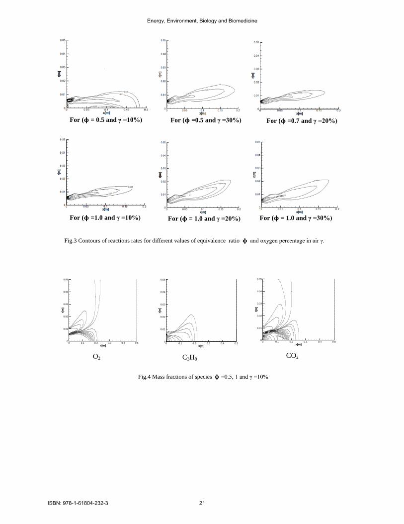
For (ϕ = 0.5 and γ =10%)

For (ϕ =0.5 and γ =30%)

For (ϕ =0.7 and γ =20%)

For (ϕ =1.0 and γ =10%)

For (ϕ = 1.0 and γ =20%)

For (ϕ = 1.0 and γ =30%)

Fig.3 Contours of reactions rates for different values of equivalence ratio ϕ and oxygen percentage in air γ.

1

34 5

6

7 8

9

9

9

10

10

11

11

12

13

14

x[m]

r[m]

0 0.1 0.2 0.3 0.4 0.50

0.01

0.02

0.03

0.04

0.05

O2

1

1

2

2

3

3

4

5

67

913

x[m]

r[m]

0 0.1 0.2 0.3 0.4 0.50

0.01

0.02

0.03

0.04

0.05

C3H8

1

2

2

3

3

3

4

4

4

5

5

5 6

6

7

7

8 8

9

10

10

11

11

12 13

14

15

15

1617 18

19

x[m]

r[m]

0 0.1 0.2 0.3 0.4 0.50

0.01

0.02

0.03

0.04

0.05

CO2

Fig.4 Mass fractions of species ϕ =0.5, 1 and γ =10%


ISBN: 978-1-61804-232-3 21

Temperature distribution

Knowing that the heat, which is released in the chemical reaction and transferred into the flowing gas including the reactant and product molecules [5], increases the temperature of this gas. In order to view the temperature distribution, the variations of temperature along the axis of burner are plotted in figure 5. It is very important to notice that the increase of φ significantly reduces the gradients so, larger temperature gradients occur in the axial direction (especially between x = 0 and about 0.20 m). The heat calculations performed for the each fuel case bring out that in the case of φ <1, the total heat per unit mass released in the combustion, Consequently, the results obtained from this figures show that in the cases of φ <1, complete combustion occurs, while in the case of φ = 1 it is very close to the complete combustion state.

VI. CONCLUSION

The combustion of propane with air in a burner was considered and the effect of the equivalence ratio and oxygen percentage in air investigated, for different numerical values. The specific conclusions derived from this study can be listed briefly as follows:

The increase of ϕ reduces significantly the reaction rate levels.

In the case of ϕ < 1, the complete combustion occurs, and the combustion in the case of ϕ = 1 is very close to the complete combustion state.

The maximum temperatures in the combustion chamber increase with the increases of γ (from 10 to 30%) and φ (from 0.5 to 1.0), respectively.

Consequently, the results of this study clearly demonstrate that Mixing hydrogen with propane causes considerable reduction in temperature levels and a consequent, reduction of CO.

REFERENCES [1] Zhou, C. Combustion. Retrieved from

http://www.eoearth.org/view/article/151315 ,(2013). [2] C.E.L. Pinho, J.M.P.Q. Delgado et al - Defect and Diffusion Forum

Vols. 273-276 pp 144-149,(2008). [3] Fluent Inc. FLUENT 6.3.26 User’s guide. (Fluent Inc), (2006). [4] Launder. B.E. and Spalding D.B. Lectures in Mathematical Models of

Turbulence. Academic Press, London, England. (1972). [5] Yapıcı, H.; Kayataş, N.; Albayrak, B.; Baştürk, Numerical study of

effect of oxygen fraction on local entropy generation in a methane–air burner .Sadhana Vol. 29, Part 6, (2004).

For (ϕ = 0.5 and γ =10%)

For (ϕ =0.5 and γ =20%)

For (ϕ =0.7 and γ =30%)

For (ϕ =1.0 and γ =10%)

For (ϕ = 1.0 and γ =20%)

For (ϕ = 1.0 and γ =30%)

Fig.5 Temperature distribution for φ = 0.5 and φ = 1.0 at different values of γ.


ISBN: 978-1-61804-232-3 22

NOMENCLATURE

Latin symbols

Greek symbols

kjδ ε

Kronecker delta turbulent energy dissipation rate

Equivalence ratio Viscous dissipation Air excess ratio Oxygen percentage in air

µ Dynamic viscosity ρ

Density Tangential direction

Kρ σij

Density of the species k Tensor of the constraint in plan i and the direction j

τ Τij

Stress tensor Tensor of the viscous constraints

CFD Cμ, Cε1, Cε2 fk,j

H

Computational fluid dynamics Coefficients in k–ε turbulence model species K in the direction i Enthalpy

,s kh K L

enthalpy of species Turbulent kinetic energy Length of burner

P

R

Pressure Heat transfer rate Universal gas constant

RNG Renormalization group r Radial distance

Inner radius of air inlet Outer radius of air inlet

T Temperature Yk Mass fraction of the species k


ISBN: 978-1-61804-232-3 23

Abstract—Up to now, the Chilean Energy system has fulfilled

the energy needs of Santiago de Chile considerably well. However, development trends of the current system impose significant future risks on the energy system. A detailed sustainability analysis of the energy sector of the Metropolitan Region of Santiago de Chile was conducted, using selected energy indicators and a distance-to-target approach. Risks for the sustainable development of the energy sector are detected, such as increasing concentration in the energy sector, import dependency for fossil fuels and increasing CO2 emissions from energy production. Options towards a more sustainable development of the Megacity of Santiago within the national Chilean energy system are asssessed, such as the enhancement of energy efficiency and an increased use of renewable energies.

Keywords—future energy situation, indicators of sustainability,

scenarios, sustainable development in developing countries

I. INTRODUCTION

Chile’s energy system is characterized by a strong growth as well as a high degree of privatization and economic concentration of energy service providers, which are controlled by the National Energy Commission (CNE) and the Energy Ministry. The total energy use in Chile (primary consumption) increased from 789 PJ (Petajoule) in 1999 to 1,593 PJ in 2012 [1], an annual average growth of 5.6%. This surge in energy consumption is for the most part a result of population growth, a highly dynamic economic development, and deficiencies in the effective use of energy resources. Approximately three quarters of the primary energy is based on fossil energy resources, which are almost completely imported from abroad.

The energy consumption of the Santiago Metropolitan Region (SMR) is dominated by the traffic sector accounting for 38% of final energy. This is followed by industry (27%), households (22%), and trade and services (13%) (data based in own calculation on [2]). By taking a closer look at the distribution of the final use of energy in terms of energy sources, it can be seen that – especially due to the energy use in the traffic sector – oil derivatives account for almost half of the final energy consumption. The other half is more or less equally distributed between gas and electricity.

The SMR can cover only 25% of its electricity demand on its own; therefore 3/4 of the electricity has to be imported. In the SMR 50% of the power is generated by fossil-fired thermal power plants, 50% by hydroelectricity.

Industry consumes the largest share of the electricity in the SMR (30%), followed by households (26%), and trade (22%). Mining accounts for 7%, agriculture for 2%, and the other sectors for 13% [3]. The power consumption per capita in the category “households” varies considerably in the different districts of Santiago. While people in Vitacura

– one of the municipalities with the highest average household income – use around 1,200 kWh electricity per capita and year, people in the “poorer” municipalities Alhué and El Monte only consume less than 360 kWh [4].

II. ENERGY SCENARIOS

In a first step two framework scenarios for the years 2030 habe been developed and the interrelations between the framework scenarios and the energy sector were analyzed. This was the starting point for the development of energy scenarios (according to [5]).

The future development of the indicators was estimated and assessed in the framework of these energy scenarios, partly based on the MESAP/PlaNet model (see [6]). The parameters which were included in the modeling are presented in table 1.

Table 1 Role of selected energy parameters in the energy scenarios 2030 (source: based on [7])

III. STAKEHOLDER INVOLVEMENT

In the course of the framing project “Risk Habitat Megacity”, a joint German-Chilean research initiative [8], 30 experts from research, federal and regional authoritities, and the industry were interviewed. These interviews provided important information on the data basis and the current situation, but also on the assessments of the future of the energy supply in Santiago and Chile and thus also for

Indicator based Sustainability Analysis of Future Energy Situation of Santiago de Chile

Volker Stelzer, Adriana Quintero, Luis Vargas, Gonzalo Paredes, Sonja Simon, Kristina Nienhaus, Jürgen Kopfmüller

Area BAU

(Business as usual)

CR (Collective

Responsibility)

MI (Market

Integration)

Role of hydropower

Realization of the large-scale

plant HidroAysen

Focus on small hydroelectric power plants

Realization of the large-scale

plant HidroAysen

Role of non-conventional renewable energy carriers

Implementation of agreed

target values (5% for 2010 / 10% for 2024)

Strong increase of

combined heat and power, wind, solar, geothermal

energy, biomass

Intensified increase in

power generation by wind and solar

panels

Role of fossil fuels

Further investments in

fossil fuel power plants

Gas as backup for renewable

energies

Further investments in

fossil fuel power plants

Transport sec-tor: share of electric vehicles in all cars registered

6% 10% 10%


ISBN: 978-1-61804-232-3 24

the further development of the scenarios. A stakeholder workshop was held at the Economic

Commission for Latin America and the Caribean (ECLAC) in Santiago. The aim of the workshop was to discuss indicators and target values as well as scenarios. During the workshop, the 20 participants from universities, authorities, and the industry entered into – in some cases very lively – discussions, especially concerning the indicators.

One of the results of the participation process was, that nuclear power is no option for Chile because

a. the high risk of disastrous earthquakes, b. the huge investment and follow up costs of the

technology and c. the very high national potential on renewable energy

with very low follow up costs. The energy results were presented in a concluding

workshop. Here especially the presented options for action were topics for discussion.

In addition, the results were included into the dialog of the regional government of the metropolitan region (GORE) for the development of a regional “politica de energies limpias”.

IV. SUSTAINABILITY ANALYSIS IN THE ENERGY SECTOR

A comprehensive set of 44 indicators was compiled on this basis of an analysies of international literature (see [9]). Then 16 “core sustainability indicators” were chosen from this list, especially regarding the appropriate representation of the rules of sustainability of the integrative concept of sustainable development [10]. Finally the following 8

indicators for the assessment of scenario results were chosen primarily based on the criteria (a) possibility to determine target values for the indicators and (b) availability of SMR data:

1. Share of rural households with no access to electricity

2. Duration of electricity supply interruptions 3. Total primary energy consumption 4. Energy intensity estimatied as: Energy per GDP 5. Share of renewable energies in electricity

production 6. Energy-related CO2 emissions per capita 7. Energy import dependency estimatied as:

Percentage of primary energy use based on imported energy

8. Degree of economic concentration in the energy sector

Where no sufficient data was available for the SMR,

national or regional values were collected for the respective indicators. Target values were identified for all indicators based on existing local, regional, or national values; if this was not possible, scientific expertise was taken as a basis.

Table 2 Scenario results = target reached, ☹ = more to do

Indicator Unit Current value

Target value 2030

BAU 2030

CR 2030

MI 2030

Share of rural households with no access to electricity in the SMR

% 0.4 (2008)

0.0 0.0 0.0 0.0

Duration of electricity supply interruptions in SMR

h 2.8 (2008)

0.0 0.6 0.2 ☹ 0.4 ☹

Total primary energy consumption

PJ 497 (2007)

As low as posible

880 ☹ 680 824 ☹

Energy per GDP 85 (2008)

≤ 40 65 ☹ 50 ☹ 60 ☹

Share of renewable energies in electricity production

% 55 (2007)

≥ 70 66 ☹ 75 76

Energy-related CO2 emissions per capita

t 4.8 (2007)

2.5 5.3 ☹ 3.1 ☹ 4.6 ☹

Percentage of primary energy use based on imported energy

% 77 (2007)

≤ 50 69 ☹ 52 ☹ 67 ☹

Degree of economic concen-tration in the energy sector

% 90 (2003)

≤ 70 90 ☹ 86 ☹ 95 ☹


ISBN: 978-1-61804-232-3 25

V. DISCUSSION OF RESULTS ACROSS SCENARIOS

The sustainability analyses of the current status and the scenario development of the indicators show a heterogeneous picture for the different scenarios. There are numerous positive developments, but also cases with large discrepancies from the target values have to be stated.

As an example, we will have a closer look at the indicator “percentage of primary energy use based on imported energy”.

One detected sustainability deficit for Chile (and the SMR) is the high dependency on fossil fuel imports, as this increases vulnerability to supply shortages and price increases. For many years Chile has been importing more than two thirds of the required energy resources. The import quota of primary energy increased from 50% in 1990 to more than 70% today. Reasons for this are the growing energy demand and the scarce reserves of conventional energy carriers in Chile.

Especially the import of natural gas from Argentina increased considerably in the past. In 2006/2007 Argentina dramatically reduced the export of natural gas to Chile by a breach of contract; this caused serious problems for Chile’s industry and private households. As a consequence, gas was to a large extent replaced by diesel and coal, which lead to a triplication of diesel imports. Also the import of oil and coal increased significantly during this period. Until 2010, approximately 1 billion US dollars were invested into two large international ports (Quintero and Mejillones) with a capacity of ca. 16 million m3 liquid gas (LNG) per day to compensate for the gas supply shortage from Argentina.

The scenario results show that different developments are possible here. Indeed the percentage share of the dependency on imports is being reduced in the BAU and MI scenarios. But the growing energy demand raises the absolute amount of imported energy raw materials. An absolute as well as a relative decrease would only be possible in CR resulting from both the significantly smaller increase of the energy demand and the stronger use of domestic renewable energies (see fig. 1) without realizing the large-scale plant HydroAisen. In this scenario a reduction of the dependency on imports to 55 % could be nearly achieved.

0100200300400500600700800900

1000

BAU CR MI BAU CR MI

2007 2020 2030

PJ

/ Y

ea

r

Imported Energy Domestic Energy

Fig. 1 Dependency of the RSM on foreign energy imports (based on [11])

VI. ENERGY POLICY FOR MORE SUSTAINABILITY

During the last years, Chile took some energy-political steps towards a more sustainable energy supply. An Energy Ministry was created on the national level, a program for energy efficiency was launched, and the regional government responsible for the SMR is working on a “politica de energía limpia” for the metropolitan region. In a future according to the CR scenario it would be possible to achieve some or come near to the sustainability target values for the selected indicators, e.g. for the indicator dependency on imports. In a world according to the BAU or MI scenario this would be different. From the foresight aspect it is therefore necessary to take further action.

One important measure is to enhance energy efficiency beyond the current activities in Chile to achieve the ojective of an efficiency increase of 20 % by 2020. In addition, in the course of the development of thermal energy production plants, gas-fired power plants should be preferred to coal-fired power plants since these can be controlled more flexibly and are therefore better suited for a continuous energy supply in combination with power plants which are based on fluctuating renewable energy carriers dependent on climatic conditions.

All in all, numerous studies conclude that non-conventional renewable energies (NCRE) in Chile have enormous potential for the future of the energy sector [12], [13] by far exceeding current policy targets. Univertsity of Chile and Technical University Federico Santa Maria estimate, that by 2025, non-conventional renewables could account for up to 30 TWh produced by almost a 6 GW installed capacity and provide more than 30 % of the total power generation [14].

The enormous potential for the use of energy from renewable sources is not equally distributed over Chile. The main reserves of energy potentials can be found for

• hydropower in the Andes • biomass in the forests in the south, in the agricultural

areas in the Central Region and the waste of the metropolitan region,

• wind power in the south, • solar energy in the north, • ocean energy in the west and • geothermal energy all over the country.

To ensure that the energy from the different regions arrives in the SMR, the infrastructure of supply lines has to be improved. Concerning the large potential of solar energy available in the north, there is the possibility of producing hydrogen or methane from solar electricity and feeding these gases into the natural gas grid which supplies the different regions of Chile coming from Argentina but is not used to capacity due to the Argentine supply shortage.

The search for and analysis of potentials from renewable energies should be started in the SMR since transport-related line losses are increasing with growing distance to the energy source. An evaluation of the suitability of existing roof areas for generating solar energy based on data


ISBN: 978-1-61804-232-3 26

from an “overflight” of the SMR would be quite easy to realize, as it is currently done in Osnabrueck (Germany) [15], but also waste material and sludge from the SMR have high potentials for a regional supply with renewable energy.

To achieve the necessary goals of increasing both the energy efficiency and the share of renewable energies in the total energy production, not only technological measures are required but also the establishment of political framework conditions which hardly exist in Chile and the SMR today. Here especially the introduction of relevant taxes and charges for the use of fossil energy carriers has to be mentioned as well as the fact that the feed-in of renewable energies into the grid should be facilitated and given priority.

Another important measure will be the analysis of the local energy resources (hydro, biomass, solar, ocean, and geothermal) of the SMR area and the two neighboring regions V and VI and to public these information for free in the internet. This could be the basis for investors to plan their energy projects for the SMR.

REFERENCES [1] Energy Ministry (2013): Balance National de Energía 2012. Santiago

de Chile. Available: http://www.minenergia.cl/documentos/balance-energetico.html.

[2] S. Simon, V. Stelzer, A. Quintero, L. Vargas, G. Paredes, K. Nienhaus, and J. Kopfmüller (2010): Thematic field: Energy. In: K. Krellenberg, J. Kopfmüller, and J. Barton (eds.): How Sustainable is Santiago de Chile? Current Performance – Future Trends – Potential Measures. Synthesis report of the Risk Habitat Megacity research initiative (2007-2011). UFZ-Report 04/2010. Leipzig

[3] National Institute of Statistics (2011): Electric generation and distribution. Historical Series: Electric distribution by sector in GWh, years 1997-2010. Available: http://www.ine.cl/canales/chile_estadistico/estadisticas_economicas/energia/series_estadisticas/series_estadisticas.php.

[4] Ministry of Planning (2006): Final Results of energy sector in Metropolitan Region, year 2006.

[5] V. Stelzer, L. Vargas, G. Parades, K. Nienhaus, and S. Simon (2009, not published): Escenarios energeticos. Backround paper: Taller ‘Sistema de Energía en Santiago 2030’. Santiago de Chile

[6] S. Simon, V. Stelzer, L. Vargas, G. Paredes, A. Quintero, and J. Kopfmüller, (2012): Energy Systems. In: D. Heinrichs, K. Krellenberg, B. Hansjürgens, and F. Martinez, (eds.): Risk Habitat Megacity: The Case of Santiago de Chile. Heidelberg. p. 183-206.

[7] S. Simon, V. Stelzer, A. Quintero, L. Vargas, G. Paredes, K. Nienhaus, and J. Kopfmüller (2010): Thematic field: Energy. In: K. Krellenberg, J. Kopfmüller, and J. Barton, (eds.): How Sustainable is Santiago de Chile? Current Performance – Future Trends – Potential Measures. Synthesis report of the Risk Habitat Megacity research initiative (2007-2011). UFZ-Report 04/2010. Leipzig. p. 12

[8] D. Heinrichs, K. Krellenberg, B. Hansjürgens, and F. Martínez, (eds.) (2012): Risk Habitat Megacity. Heidelberg.

[9] V. Stelzer, J. Kopfmüller, and S. Simon (2010): Nachhaltige Energieversorgung in Megacities. Das Beispiel Santiago de Chile. In: Technikfolgenabschätzung Theorie und Praxis, 19, 3, p. 30 - 38

[10] J. Barton, and J. Kopfmüller (2012): Sustainable Urban Development in Santiago de Chile: Background – Concept – Challenges. In: D. Heinrichs, K. Krellenberg, B. Hansjürgens, and F. Martinez (eds.): Risk Habitat Megacity. Heidelberg. p. 65-86

[11] S. Simon, V. Stelzer, L. Vargas, G. Paredes, A. Quintero, and J. Kopfmüller (2012): Energy Systems. In: D. Heinrichs, K. Krellenberg, B. Hansjürgens, and F. Martinez, (eds.): Risk Habitat Megacity: The Case of Santiago de Chile. Heidelberg. p. 183-206.

[12] International Energy Agency (2009): Chile Energy Policy Review 2009. Paris.

[13] Greenpeace International, European Renewable Energy Council, Deutsches Zentrum für Luft- und Raumfahrt, and ecofys (2009): Energy [R]evolution - a sustainable Chile energy outlook. Amsterdam.

[14] Univertsity of Chile, and Technical University Federico Santa María (2008): Estimación del aporte potencial de las Energías Renovables No Convencionales y del Uso Eficiente de la Energía Eléctrica al Sistema Interconectado Central (SIC) en el período 2008-2025. Santiago de Chile

[15] University of Aplied Science Osnabrück, and City of Osnabrück (2010): SunArea – Dachflächen für Photovoltaik in Osnabrück; Available: http://geodaten.osnabrueck.de/website/Sun_Area/viewer.htm


ISBN: 978-1-61804-232-3 27

http://www.minenergia.cl/documentos/balance-energetico.html�

http://www.minenergia.cl/documentos/balance-energetico.html�

http://www.ine.cl/canales/chile_estadistico/estadisticas_economicas/energia/series_estadisticas/series_estadisticas.php�

http://www.ine.cl/canales/chile_estadistico/estadisticas_economicas/energia/series_estadisticas/series_estadisticas.php�

http://geodaten.osnabrueck.de/website/Sun_Area/viewer.htm�

A scalable method for efficient stem cell donor HLA genotype matchdetermination

D. Georgiev, L. Houdová, M. Fetter, and P. Jindra

Abstract— Finding suitable stem cell donors comprises threeindependent processes: donor pool HLA typing, donor HLAhaplotype inference, and search for donor HLA genotypematches. For practical and technical reasons, these processesare often decoupled leading to informational losses along theway. A method is presented that eliminates some of the technicalchallenges by considering all three steps together. The methodrelies on two practical assumptions: there exists a set of commonhaplotypes and the matched target is typed at high resolution.Under these two assumptions, sufficient statistical HLA analysisof a stem cell donor pool is performed to identify donors thatmost likely match a given genotype. The presented commonhaplotype Expected-Maximization (chEM) method is scalablein the number of loci, the number of alleles, and typingambiguity, overcoming the known curse of dimensionality forthe problem of HLA haplotype inference. The practical valueis demonstrated on real world data provided by the CzechNational Marrow Donor Registry. It is shown the chEMmethod significantly reduces the field of potential matches whencompared to an existing match algorithm.

Index Terms— stem cell donors, HLA refinement, statisticalmethods

I. BACKGROUND

A brief review of the typing, resolution, and matchingprocesses is given. For the sake of simple exposition, un-necessary details are omitted. For more information see [1].

A. Typing methods and nomenclature

Donors are usually typed for up to five loci along chromo-some 6: HLA-A/B/C/DRB1/DBQ1. Typing results of donorsin a given registry bare different levels of resolution, basedon time and location of recruitment. Low level methods relyon antibody-based serological tests. Intermediate resolutionmolecular methods are based on hybridisation with sequence-specific oligonucleotide probes or PCR amplification withallele specific primers. High resolution methods are based onDNA sequencing tools, which aim to return a four digit num-ber, e.g., A*03:01 or A*03:26, describing the exact aminoacid sequence of the corresponding allelic coding region.Ambiguity regarding the amino acid sequence is possiblefor highest resolution typed donors if their chromosome paircontains an indeterminate allele combination. Decreasing thetyping resolution further increases possible allele ambiguity.

This work was supported by the grant TA CR TA01010342.D. Georgiev, L. Houdová and M. Fetter are with the Department of

Cybernetics in the Faculty of Applied Sciences, University of West Bohemiain Pilsen, Pilsen 30614, Czech Republic. [email protected],[email protected], [email protected] P. Jindra is withthe Biomedical Centre, Faculty of Medicine in Pilsen, Charles Univer-sity in Prague, Pilsen 30460, Czech Republic, and with HLA labora-tory, Czech National Marrow Donors Registry, Pilsen, Czech [email protected]

Hybridisation probes and PCR primers are targeted to aportion of the allele sequence only, and thereby merelyidentify a list of consistent alleles, e.g., A*03:01-A*30:01.Standard allele lists include entire allele groups, approxi-mately corresponding to broad antigen types, denoted by thefirst two digits in the allele number, e.g., A*03. Alternatively,specific allele sets are assigned letter codes using the WHOnomenclature [2], e.g., DRB1*15:HMYC. The following isan example typization of a donor from the Czech NationalMarrow Donor Registry (allele ambiguities, given by thenumber of possible alleles, are listed in parenthesis):

A B C DRB168:JAHD(16)

27:HMHK(13)

07(348) 11:HMXW(12)

03:JAGH(50)

07:HMGA(31)

01(90) 15:HMYC(17)

The above donor is heterozygous at the four typed loci,where the loci HLA-A/B/DRB1 are typed at intermediateresolution and HLA-C is typed at low resolution. The locusHLA-DQB1 is not typed implying it has 509 possible alleleson each chromosome. Such a donor has (at high resolution)1.9 × 1010 possible haplotypes, 5.3 × 1017 possible HLAgenotypes, and 4.3 × 1018 possible haplotype pairs. If thetyping data is truncated to low resolution, then the ambi-guity is reduced significantly: 224 possible haplotypes, 196possible genotypes, and 1568 possible haplotype pairs. If, inaddition, the haplotype is limited to the typed loci, then (atlow resolution) there are 16 possible haplotypes, 1 possiblegenotype, and 8 possible haplotype pairs.

B. Statistical methods for HLA refinementAdditional typization to increase HLA resolution and re-

duce the ambiguity (at high resolution) is rarely implementedfor a large pool of donors. Instead statistical methods areused to refine a given HLA typing. In the simplest approach,allele frequencies are calculated independently at each locusand used to compute genotype probabilities without account-ing for linkage effects. Real world populations, however,share common ancestry and exhibit nonuniform mating pat-terns that lead to linkage disequilibrium manifested in allelecorrelations across HLA haplotypes [3].

There is no gold standard for probabilistic haplotypemodelling generally accepted by the stem cell donor reg-istries. Three types of methods are available [1]. The Clark’salgorithm approaches haplotype modelling parsimoniouslybeginning with the list of homozygous haplotypes and then


ISBN: 978-1-61804-232-3 28

expanding the list in an ad hoc manner until all donorgenotypes are resolved. Expected-Maximization (EM) meth-ods consider all possible genotype deconstructions and lookfor haplotype probabilities of the general population thatmaximise the likelihood of drawing the donor pool. Bayesianmethods rely on more detailed models of population geneticsto stochastically generate population haplotypes and empiri-cally estimate haplotype frequencies [4].

Choice of method is determined by several factors. UsuallyEM and Bayesian methods outperform the Clark’s algorithm.Furthermore, EM methods have better convergence proper-ties, include simpler parametrizations, but scale poorly withthe number of loci, the number of alleles, and the alleleambiguity. Bayesian methods potentially have lower compu-tational complexity but lack the implementation simplicity ofthe EM methods. For this reason, most stem cell registriesimplement their own version of the EM method [5], [6].Below is a summary of the standard EM algorithm used forhaplotype modelling.

The haplotype probability model is iteratively computedas follows.

1) Haplotype set H = {h1, ..., hn}: let d be the numberof donors and construct a set of haplotypes by decon-structing the donor genotypes.

2) Initialization of p0 (k) , L0, s, S, ε: initialise the proba-bility p0 (k) of haplotype hk appearing in the populationand the likelihood function L0 = 0. Set the iterationcount s = 0, the maximum iteration count S, and theconvergence threshold ε.

3) Start: while s ≤ S, repeat the following steps,otherwise, terminate the algorithm without convergence.i) For k = 1, ..., n, count the occurrence nk of haplo-

type hk.

nk =

d∑i=1

n∑j=1

(1 + δkj)P (hk, hj |gi) , (1)

where δkj is the delta function, gi ={(hi11, hi12) , (hi21, hi22) , ..., (hir1, hir2)} is the ithdonor’s genotype deconstructed into all possiblehaplotype pairs, and

P (hk, hj |gi) =ps (k) ps (j)

P (gi), (2)

P (gi) =r∑j=1

ps (hij1) ps (hij2) . (3)

ii) For k = 1, ..., n, compute the next iteration of thehaplotype probabilities and the likelihood function:

ps+1 (k) =nkn, (4)

Ls+1 =d∑i=1

log (P (gi)) . (5)

iii) Check the convergence criteria: if |Ls+1 − Ls| > ε,increment s and return to (i), otherwise, terminatewith convergence.

The limitation of the standard EM algorithm is in Step 1.Only a small percentage of donors are typed at high resolu-tion. Deconstructing genotypes of donors typed at interme-diate or low resolution into all possible haplotypes generatesa prohibitively large haplotype set. Hence, computationalcomplexity attributed to typing ambiguity for actual donorpools is overly prohibitive for simple deployment of thestandard EM algorithm [1]. In practice, EM algorithmsare either executed at low resolution, where there is littleambiguity (see example above), or executed heuristically toexplore specific linkages in partial haplotypes.

C. Donor matching

A donor is a match for a given patient if they sharethe same genotype. With some exceptions, a patient istyped at high resolution and hence ambiguity arises almostexclusively on the donor side. Two steps are commonly usedto resolve this ambiguity. A simple solution is to converttyping data to a lower resolution, e.g., antigen split groups,where there is little ambiguity and common populationhaplotypes may be used to predict the missing information.Alternatively, the donor genotype is matched only across thetyped loci, generating so called 6/6, 8/8, and 10/10 matches.Such matches are of the boolean type, a donor is classifiedas a potential match if their partially genotype possiblyequals the partial genotype of the patient. Effectively, useof probabilistic haplotype models for HLA refinement isignored.

II. RESULTS

The results in this paper comprise a method that over-comes the greatest shortcoming of the EM algorithm, itscomputational complexity caused by typing ambiguity athigh resolution. Below the common haplotype EM (chEM)method is introduced and its scalability demonstrated in adeployment on a large portion of CNMRD donors typedat various loci and various resolution levels. A five-lociprobabilistic model of the Czech population is derived. Inaddition, the model and the introduced tools are shown tooutperform existing intermediate resolution methods in donormatching.

Assumption. The chEM method is based on the followingassumptions.

A1) The list of common haplotypes is known.A2) Patients are typed at high resolution.

Assumption 1 is likely considering most newly discoveredalleles are rare [7]. Sequencing methods have also becomeaffordable enough to where Assumption 2 is now generallytrue.

A. Common haplotype probability model

The derived method differs from the EM algorithm ap-proach described in Section I-B in the following fundamentalway. The haplotypes are decomposed into those that arecommon, denoted simply by H = (h1, ..., hn), and those thatare rare, denoted by HR =

{hR1 , h

R2 , ...

}. Rare haplotypes


ISBN: 978-1-61804-232-3 29

either contain rare alleles (possibly still unknown) or a rarecombination of alleles and as a result have a much lowerprobability of arising in the population.

The EM algorithm is modified and implemented in thefollowing way to efficiently compute the common haplotypeprobability model.

1) Haplotype set H = {h1, ..., hn}: the set of commonhaplotypes is given.

2) Initialization of p0 (k) , L0, s, S, ε,M : Initialise p0and L0 as above. Set the values of s, S, and ε asabove. Set M to be the number of maximum allowablehaplotypes per donor.

3) Construct the relevant donor pool D = {1, ..., d}: adonor in the general pool is deemed relevant as follows.i) Set the iteration count a = 1 and initialise the donor’s

list of potential haplotypes Hp to H .ii) Consider all alleles possible for the donor at the ath

locus and exclude from Hp any haplotype that doesnot share one of these alleles.

iii) If the size of Hp ≤ M , the donor is deemedrelevant, otherwise, if a is less than the number ofloci, increment a and return to the previous step. If ais equal to the number of loci, the donor is deemedirrelevant.

4) Construct the set of common haplotype pairs gci , i ∈{1, ..., d}: for donor i, first select one of the pre-computed common haplotypes, then search for its pair.The search is done in the same way as when identi-fying relevant donors (Step 3), the exception being thepossible alleles are now limited to the complementarychromosome copies.

5) Continue as in Step 3 of the traditional EM algorithmdescribed above with gc substituted for g.

Limiting the EM algorithm to the common haplotype listreduces the computational complexity in a number of ways.First, model complexity, i.e., the number of potential haplo-types, is explicitly bounded. As a result, the computationalcomplexity attributed to typing ambiguity (represented by themaximal number of donor haplotypes M ) can be indepen-dently controlled. In the standard EM algorithm, the numberof donor haplotypes grows with M and the number of donorsd. Hence to reduce the model complexity, one must considereither high resolution donors or limit the number of donors.Lastly, a relevant donor must not necessarily be typed at highresolution. Their genotypes must merely deconstruct into anacceptable number of common haplotypes. In the case studybelow, for M = 150 the number of relevant donors d fromCNMRD is equal to 23, 819(54%oftheentiredatabase). Inthe standard EM algorithm, any donor typed at intermediateresolution or below for 2 out of the 5 loci would be deemedirrelevant. In the present, there are only 3,339 (7.6% of theentire database) such donors in the CNMRD. Hence, limitingthe model to the common haplotypes greatly increases thestatistical relevance of the results for fixed donor ambiguity.

B. Matching genotypes

The chEM algorithm presented in Section II-A only com-putes the probability model for the common haplotypes.What isn’t yet clear is how this model is useful in matchingdonors to patients, especially when the patient has a rarehaplotype. We start by again considering the donor andpatient genotypes deconstructed into sets of all possiblehaplotype pairs gD and gP , respectively.

The standard search for a donor with a genotype thatlikely matches the patient’s genotype involves processingthe general donor pool and for each donor evaluating theconditional probability

P (gP |gD) =P (gP ∩ gD)P (gD)

, (6)

where the Hardy–Weinberg equilibrium is used to computethe probabilities on the right hand side of the equation.For this, however, we need a full probability model ofall possible haplotypes in the donor pool. The chEM al-gorithm of Section II-A only computes the probabilitiesP (hk|donor pool contains 0 rare haplotypes), written heresimply as P (hk|0).

If the occurrences of different rare haplotypes in the donorpool are equally likely and statistically independent and ξ isthe probability the donor pool has at least one rare haplotype,then the true probability is given by

P (hk) = P (hk|0) (1− ξ) +∞∑i=1

P (hk|i)(

ξ

1 + ξ

)i. (7)

Under assumptions A1 and A2, the probability ξ is small.Hence we can approximate the match probability in Equa-tion 6 by its Taylor series approximation.

P (gP |gD) =∞∑i=0

ξi

i!

∂iP (gP |gD)∂ξi

∣∣∣∣ξ=0

(8)

Three scenarios are possible and characterised by thedominant terms in the above Taylor series.

Scenario 1) If gP includes at least one common haplotypepair, then

P (gP |gD) ≈∑

(h1,h2)∈gP ∩gDP (h1|0)P (h2|0)∑

(h1,h2)∈gDP (h1|0)P (h2|0) .

Scenario 2) If gP includes no common haplotype pairs andat least one pair with one common haplotype, then

P (gP |gD) ≈∑

(h1,h2)∈gP ∩gDP (h1|0)P (h2|1)+P (h1|1)P (h2|0)∑

(h1,h2)∈gDP (h1|0)P (h2|0) .

Scenario 3) If gP includes only rare haplotype pairs, then

P (gP |gD) ≈∑

(h1,h2)∈gP ∩gDP (h1|1)P (h2|1)∑

(h1,h2)∈gDP (h1|0)P (h2|0) .

The above facts suggest that to approximate the donor matchprobabilities, all rare haplotypes would have to be appendedone at a time to the haplotype model. This is true if theprobabilities themselves are of interest, however, for thepurposes of finding the best donor, only the ordering of theprobabilities is required.


ISBN: 978-1-61804-232-3 30

Note, for any patient typed at high resolution, it is true thateither a donor’s possible haplotype pairs include ALL of thepatient’s possible haplotype pairs or NONE of the patient’shaplotype pairs. Correspondingly divide the general donorpool into the potential matches denoted by DP and the rest,where any donor i ∈ DP satisfies gi ⊇ gP and any donorj /∈ DP satisfies gj ∩ gP = ∅.

Any two donors i, j ∈ DP satisfy the equality gi ∩ gP =gj ∩ gp. As a result, the numerator of the match probabilityapproximations in the three scenarios is constant for alldonors in DP . This leads to the following fact regardingordering of matching donors.

Fact 1. Consider the set DP of donors possibly matching agiven patient’s genotype, represented by the set of haplotypepairs gP . As the probability ξ of a rare haplotype in thedonor pool approaches 0, for any two donors i, j ∈ DP ,

P (gP |gi) > P (gP |gj) if and only if P (gi|0) < P (gj |0) ,(9)

where P (gi|0) and P (gj |0) are the genotype probabilitiesconditioned on there being no rare haplotypes in the donorpool.

The above fact states that only the common haplotypemodel is required to order the potentially matching donors.The match probability can be estimated using the commonhaplotype model only when the patient genotype can bereconstructed using common haplotypes. Otherwise, the hap-lotype model would have to be expanded to include all rarehaplotypes.

C. CNMRD derived haplotype model of the Czech popula-tion

The haplotype model was derived for a CNMRD donorpool satisfying the ambiguity criterion introduced in thechEM algorithm. CNMRD includes 44,256 donors, of which39,403 (90%) are typed for HLA-A/B/DRB1 loci and 70%have some serological typization. Donor ambiguity was lim-ited to at most 150 possible common haplotypes, met by 54%of the registry’s donors. Donors deemed overly ambiguousto yield significant statistical information included many thatwere typed for only two loci, e.g., HLA-A/B, and had up to20 thousand possible common haplotypes.

The list of common haplotypes making up the derivedhaplotype model included 64, 800 entries taken from [8].This was assumed to be the list of all common haplotypescalled for by Assumption 1. In deployment, however, thepossible genotypes of numerous donors from the selecteddonor pool could not be reconstructed using the listedcommon haplotypes. All such donors had serologically typedHLA-C. Consultation with field experts revealed that olderserological typing methods for HLA-C have a 30% error rate.Once HLA-C typing was ignored for these donors, commonhaplotype pairs were successfully used to reconstruct at leasta single genotype for every donor in the selected pool.

A prototypical algorithmic implementation was built usingthe open source PosgreSQL database system. The conver-gence criterion ε was set to 3.8 × 10−4% of the finallog-likelihood value. Moreover, a threshold, below which aprobability was taken to equal zero, was set to 1× 10−8. Anaive implementation of the chEM algorithm converged in22 iterations in approximately 36 hours. While this executiontime seems excessive, the common haplotype model doesnot need to be re-computed in real time. In addition, muchfaster convergence is expected when performing only modelupdates.

The final computed model included 11,458 haplotypeswith positive probability. The following is a list of the fivemost common haplotypes and their probabilities identifiedfor the Czech population.

A B C DRB1 DQB1 Prob.01:01 08:01 07:01 03:01 02:01 0.05003:01 07:02 07:02 15:01 06:02 0.01202:01 13:02 06:02 07:01 02:01 0.01023:01 44:03 04:01 07:01 02:01 0.00901:01 57:01 06:02 07:01 03:03 0.009

D. Validation

The method was tested on real patient case studies and thematching results were compared against outputs of existingintermediate level search tools. In searching for matches, alarger donor pool was used. Any donor typed for at leastHLA-A/B/DRB1 was considered in the search (this included90% of the donors contained in the CNRMD database).The ignored database entries include 1,595 donors typedserologically only for HLA-A/B and 3,025 donors typed forHLA-A/B/C, where often the HLA-C typing is erroneous.In practice, the minimal match criterion used is 5 out of 6matching alleles. Hence, the ignored donors are most likelynot suitable candidates. Of the donors that were includedin the search, 3,168 were typed at high resolution, 22,848were typed for HLA-A/B/C/DRB1, and 13,299 were typedfor HLA-A/B/DRB1.

The search method currently in use was implementedover 15 years ago to find matching donors using theirserological typing data. The method relies on uniform typingdata in terms of resolution and HLA loci. Therefore, typingof donors obtained using molecular methods is convertedto serological format using standard conversion tables andgenotypes are only matched across HLA-A/B/DRB1 loci. Adonor with potentially matching alleles at all three loci andboth chromosomal copies is called a 6/6 match.

The chEM method presented herein searches for matchesacross all loci, doesn’t require uniform typing data, and iscapable of finding high-resolution matches. For patients withrare genotypes, the method simply ranks the potential donors.For patients with common genotypes, the method ranks thedonors and lists their match probabilities. Nonetheless, forcomparison purposes, the method was naturally reduced tosearch for matches across the HLA-A/B/DRB1 loci.


ISBN: 978-1-61804-232-3 31

The CNMRD database 6/6 matches identified by the twomethods were compared for 100 patients chosen at random.The existing method relies on serological conversion. Henceit is expected that the presented chEM method will shrinkthe set of potential donors. The table below summarises thiscomparison study.

# RESULT

41 cases where matches were found using exist-ing method

29 cases where matches were found using thechEM method

21 cases where chEM decreased the number ofmatching donors

As expected, in the majority of cases, the chEM methodreduced the set of matching donors. In no cases, the chEMmethod identified matching donors not identified by theexisting method. Out of the cases where the chEM methoddecreased the number of potential matches, the averagereduction was approximately 25.8%.

Below is an example patient and the most likely 6/6matching donor identified by the chEM method. Despite thedonor being typed only at intermediate resolution (the donorhas 2 × 1020 possible genotypes) for the three loci HLA-A/B/DRB1, the probability of a 6/6 match is equal to 0.97.Using the chEM method, a search for 10/10 matches wasalso performed. The same donor was also the most likely10/10 match with match probability equal to 0.11.

A B C DRB1 DQB1

Patient 02:01 27:05 01:02 01:01 05:0102:01 38:01 12:03 13:01 06:03

Donor

02:KDMZ

27:KCXM

13:KEGB

02:KDMZ

38:KCXZ

01:KEFC

III. DISCUSSION

One of the fundamental limitations of statistical HLAtyping resolution refinement is the computational complexity.Typing ambiguity present in donor pools is almost alwaysprohibitive forcing the use of heuristic reductions. Herein wedemonstrate that haplotype models used for refinement needto be only defined over the common haplotypes. As longas the probability of rare haplotypes is sufficiently small,potential donor matches can be identified and sorted purelyon the bases of the common haplotype model. A prototypicalimplementation of the method was proven in terms of robust-ness and computational speed for the CNMRD database ofover 40 thousand donors. The method was further validatedin matching donor search case studies, where the resultsproduced using existing donor search tools were significantlyrefined in the majority of cases.

REFERENCES

[1] J. Listgarten, Z. Brumme, C. Kadie, G. Xiaojiang, B. Walker, M. Car-rington, P. Goulder, and D. Heckerman, “Statistical resolution ofambiguous HLA typing data,” PLoS Comp. Biol., 2008.

[2] Nomenclature for Factors of the HL-A System, WHO nomeclaturecommittee, 1968.

[3] A. Degioanni, P. Darlu, and C. Raffoux, “Analysis of the french nationalregistry of unrelated bone marrow donors, using surnames as a toolfor improving geographical localisation of HLA haplotypes.” EuropeanJournal of Human Genetics, 2003.

[4] M. Stephens, N. J. Smith, and P. Donnelly, “A new statistical methodfor haplotype reconstruction from population data,” American Journalof Human Genetics, 2001.

[5] D. Steiner, “Probabilistic matching in search for unrelated hematopoi-etic probabilistic matching in search for unrelated hematopoietic stemcell donors,” Ph.D. dissertation, Czech Technical University in Prague,2013.

[6] Z. S. Qin, T. Niu, and J. S. Liu, “Partition-ligation–expectation-maximization algorithm for haplotype inference with single-nucleotidepolymorphisms,” American Journal of Human Genetics, 2002.

[7] P. Jindra, P. Venigová, L. Houdová, and K. Steinerová, “A novel HLA-Anull allele (A*02:395N) with stop codon in exon 2 generated by singlenucleotide exchange,” Tissue Antigens, 2013.

[8] L. Gragert, A. Madbouly, J. Freeman, and M. Maiers, “Six-locus highresolution hla haplotype frequencies derived from mixed-resolution dnatyping for the entire us donor registry,” Human Immunology, 2013.


ISBN: 978-1-61804-232-3 32

Abstract— Magnetic Resonance Image is one of technologies

used for diagnosing brain cancer. Radiographer use information get

from MRI images to diagnose the disease and plan further treatment

for the patient. MRI images are always corrupted with noise.

Removing noise from images is crucial but it is not an easy task.

Filtering algorithm is the most common method used to remove

noise. Segmentation technique is normally used to process image in

order to detect abnormality happen specifically for brain. But

segmentation alone would best to implement when the images is in

good condition. In the case where the images are corrupted with

noise there are pre processing steps need to be implemented first

before we can proceed to the next task. Therefore, in this project we

proposed a simpler method that can denoise and at the same time

segment the image into several significant region. The proposed

method is called switching-based clustering algorithm. The algorithm

is implemented on MRI brain images which are corrupted with

certain level of salt-and-pepper noise. During the segmentation

process, the results showed that the proposed algorithm has the

ability to minimize the effect of noise without degrading the original

images. The density of noise in the MRI images made varies from 5%

to 20%. The results are compared with conventional clustering

algorithm. Based on the experimental result obtained, switching-

based algorithm provided a better segmentation performance with

fewer noise effects than conventional clustering algorithm.

Quantitative and qualitative analysis showed positive results for the

proposed switching-based clustering algorithm.

Keywords— Magnetic Resonance Image (MRI), Image

processing, Image Segmentation, Switching-based Clustering

Algorithm, Salt-and-Pepper Noise.

I. INTRODUCTION

EDICAL imaging is an important instrument in

medicine. Magnetic Resonance Image (MRI) is an

imaging method commonly used in medical setting to generate

high quality images and provide more effective information of

the inside of the human body[1, 2]. It presents the clinician

S. N. Sulaiman is a Senior Lecturer at Faculty of Electrical Engineering,

Universiti Teknologi MARA (UiTM), 13500 Permatang Pauh Penang,

Malaysia. (Phone: +604 3822619; fax: +604 3822810; e-mail:

[email protected]).

S. M. Che-Ishak, was undergraduate student at Faculty of Electrical

Engineering, Universiti Teknologi MARA (UiTM), 13500 Permatang Pauh

Penang, Malaysia. (e-mail: [email protected]).

I. S. Isa. is a Lecturer at Faculty of Electrical Engineering, Universiti

Teknologi MARA (UiTM), 13500 Permatang Pauh Penang, Malaysia (e-mail:

[email protected]).

N. Hamzah is a Lecturer at Faculty of Electrical Engineering, Universiti


[email protected]).

with a number of corresponding quick, precise and flexible

diagnostic tools. Magnetic Resonance Image is supposed to be

very potential for precise measurement of organ anatomy in a

simply way. It is very important to obtain correct image in

order to make easy the accurate observations for a given

application in medical image processing [3]. Besides that, it

can also be used to determine the abnormal and normal types

of brain.

Unfortunately, medical images are prone to be corrupted by

noises. Noise is the unwanted signal present in original signal.

It generated in any form or any time. A noisy image can be

caused by a faulty memory, a faulty sensor in camera and noise

in a channel during transmission. In medical images, salt-and-

pepper noise is a typically noise seen on images. It is randomly

occurring black or white (or both) pixels over the images. This

degradation can be caused by errors in data transmissions and

disturbances in the images [4]. Low quality of image is a

problem for efficient feature extraction, analysis, and

quantitative measurements. Removing noise from medical

image is the major task and to denoise the image is not easy.

Denoising should be used to improve the image quality for

more precise diagnosis [5, 6].

Denoising means minimize the noise in homogenous area

without degrading the image details. Denoising is commonly

used for post processing method like restoration, segmentation,

classification, pattern analysis and others [7]. Conventionally,

noise images have to undergo pre-processing step before being

subjected further specifies to analysis. Filtering algorithm is

the most common method used to remove the noise as pre-

processing. In medical imaging, image filtering algorithm

technique is used to enhance image quality, increase visibility

which helps in the diagnostic process [5]. However those

methods are only for filtering for noise removal and applied

the further task on the images as image segmentation [8].

Denoising based segmentation method is proposed to be used

to remove the noise and at the same time segment the image

into several significant regions.

Segmentation algorithm is the method of subdivides an

image into different regions [9]. It is widely used in the field of

biomedical application [1]. The image segmentation is mainly

used to simplify or change an image into something that is

more meaningful and easier to analyse without degrading the

fine details image s[2]. The radiologists used this method to

segment the input medical image meaningful regions.

Clustering is the process classification design or pattern of

Denoising of Noisy MRI Brain Image by Using

Switching-based Clustering Algorithm

Siti Noraini Sulaiman, Siti Mastura Che Ishak, Iza Sazanita Isa, Norhazimi Hamzah

M


ISBN: 978-1-61804-232-3 33

group which is of similar characteristic for further analysis

[10] and widely used for segmentation of MRI brain images.

Besides that, clustering algorithm are planned with the

objective to create better segmentation [11]. Clustering

algorithm figure the typical each cluster in image

segmentation. Then, segments the image by categorize each

pixel in the closet cluster according to a distance metric. A

good results segmentation can be achieved through clustering

technique [9]. In MRI brain images, segmentation technique is

performed to detect abnormality in brain. It is used to identify

three normal tissue such as GM (Gray Matter), WM (White

Matter), and CSF (Cerebrospinal Fluid).

In this paper, a new method to minimize noise in the

corrupted MRI brain images is proposed i.e. by using a

clustering algorithm. The method is known as switching based

clustering algorithm [8]. Salt-and-pepper is the fix value

impulse noise. It can severely damage data embedded or the

information in the original image. For conventional method,

when salt-and-pepper noise is occur on the MRI brain images,

segmentation can only be applied after complete pre-

processing tasks such as algorithm. New clustering algorithm

for the segmentation of noisy images is proposed to tackle this

problem. The switching-based clustering algorithm allows the

clustering algorithm to segment the noise image of low-density

salt-and-pepper noise without any prior filtering stage. The

difficulty of the process can be reduced by include two

independent process (i.e. noise filter and segmentation into one

method [8, 9].

This paper organized as follow. In section II explain the

switching-based clustering algorithm. Section III describes the

proposed methodology. Section IV explains the experiments

results and analysis and section V conclusion of paper is

discussed.

II. SWITCHING-BASED CLUSTERING ALGORITHM

New method of clustering based segmentation method is

proposed for images corrupted with different level salt-and-

pepper noise. The method known as switching-based

clustering algorithm [8] which is proposed to minimize salt-

and-pepper noise sensitivity in segmentation, at the same time

increase the potency of the clustering with respect to noise.

The algorithm is chosen due to its ability to minimize the noise

during the segmentation process without corrupting the fine

details of image. The method is divided into two stages. The

first stage is the noise detection stage to scan the location of

salt-and-pepper noise and record its intensity. The second

stage is the clustering process.

In the most clustering algorithm, the algorithms are very

sensitive to noise where no spatial information of the image is

considered. To minimize the noise sensitivity of the clustering

algorithm, the spatial information of the image is commonly

considered. This concept is implemented in switching-based

AFKM clustering algorithm therefore it is implemented in

MRI brain images. The whole implementation of switching

AFKM clustering algorithm will be explain in this section as

what had stated by [8].

A. Noise Detection

The main purposed is to recognize the intensity of the

‘noise-pixels’ in this stage. Then, place the positions. In the

interval [0,255], an 8-bit gray scale digital image is considered

with 256 gray levels. Normally, the salt-and-pepper noise has

obtained on the high-end and low-end intensities [12-14]. It

can be either positive or negative value. The intensity value for

the positive impulse is close to 255 (i.e., known as the salt

appear white), and the negative impulse with the intensity

value of close to 0 (i.e., known as the pepper appears black).

‘Noise pixels’ in the image can be recognizing by these salt-

and-pepper noise intensities. According to [13, 14], a binary

noise mask N(i, j) will be produced to mark the location of

‘noise-pixels’ by the following :

where X(i, j) is the pixel at the location (i, j) with the intensity

X,N( i , j) = 1 stand for the ‘noise free pixels’ to be retained in

the next clustering stage and N(i, j) = 0 stand for ‘noise pixels’.

Lsalt and Lpepper are the local maxima representing the highest and

lowest intensities.

B. Segmentation via AFKM Clustering

After the noise and noise free pixels is being recognized and

identified, the next step i.e. segmentation via clustering is then

commence. In this paper, as mention before the AFKM

clustering algorithm [15] is chosen to be implemented on the

MRI-brain images. The steps for AFKM is explain as follows.

Consider an image with X × Y pixel as the number columns

and Y pixels as the number of rows. Let vt be the t-th data and

ck is the k-th center. The aim of AFKM algorithms is to

minimize the objective function given as follows:

where . stands for distance measure that is normally

considered as the Euclidean norm. All data are assigned to the

nearest centre based on the Euclidean distance. Then, m, the

fuzziness exponent, is an integer, m>1. The new position for

each centre is calculated using:

1

0),( jiN

otherwise

peppersalt Lor L X (i, j)if

(1)

cn

k

J

1

N

t

mk t

M

1

2

kt cv (2)

N

t

mk

N

t

tmk

k

t

t

M

vM

c

1

'

1

'

(3)


ISBN: 978-1-61804-232-3 34

The value of mk t

M is simplified in the iteration according

to [15]:

mk

mk

mk ttt

MMM '

(4)

As kk

t

ecM mk

(5)

where is a designed constant with value between 0 and 1

and typically set to 0.1. Then, the value of ke is the error

Belonging noise. The degree of Belongings, ke is the degree of

Belongingness, kB is calculated by[15]:

BBe kkkˆ (6)

where

kB is the normalized value for degree of belongingness.

mk

k

t

k

M

cB (7)

The whole implementation of switching-based AFKM can be

refer to [8] and [15].

III. PROPOSED METHODOLOGY

This project is focused on noise removal for medical images

(MRI brain) but at the same time segment the images. The

implementation of the project is simplified in flow chart

below:

Figure 1 : Methodology

The proposed method to denoise the MRI brain images is by

using switching AFKM. In this paper, five of MRI images are

chosen from the tested images and to be used to analyse the

performance of the proposed algorithm. These images are

consists normal and abnormal brain as shown in Figures 2(a)

to 2 (e) respectively. The images then are inserted with

different level of salt-and-pepper noise (by simulation) using

MATLAB 2010 image processing toolbox. The level of noise

inserted is between 5% to 20%. After that, the corrupted

images is tested with switching-AFKM and compared with the

conventional segmentation method i.e the AFKM algorithm.

The result are evaluated both qualitative and quantitative

analysis.

(a) (b) (c)

(d) (e)

Figure 2: The original image (a) Normal 1, (b) Normal 2,

(c) Normal 3, (d) Abnormal 1 and (e) Abnormal 2

IV. EXPERIMENTAL RESULTS AND ANALYSIS

Original MRI brain images were performs on the results as

a reference images. The salt-and-pepper noise is added to the

images. The corrupted images are 5% to 20% density of salt-

and-pepper noise. The noises have to remove to get better

results. Denoising is perform by using the proposed algorithm

(switching-based clustering algorithm) and compare with

conventional clustering algorithm. Comparison being made

based on the qualitative and quantitative analysis.

A. Qualitative Analysis

Segmented images are evaluated in this analysis. This

analysis is depends on the type of purpose on the MRI brain

images. The results of qualitative will be different for

different application on the images. This is because each

method has the good quality and performance of

segmentation.

In experiments, the proposed switching-based clustering

algorithm on normal and abnormal MRI brain images are

corrupted with different levels densities of salt-and-pepper

noise. Its results were compared with conventional-based

clustering algorithm. The main goal is to determine the

performance of the proposed algorithm should minimize the

effect of salt-and-pepper noise during segmentation process.

All images are segmented into three clusters.

The segmentation results for Normal 1, Normal 2, Normal

3, Abnormal 1 and Abnormal 2 images are shown in Figures 3,

4, 5, 6, and 7 respectively. Image (a) represents the original

Start

Obtain MRI brain images from website

Insert noise by simulation using

MATLAB

Switching AFKM Conventional Segmentation

(AFKM)

Compare performance

Analyse performance of the method

End


ISBN: 978-1-61804-232-3 35

image, image (b) is a noisy image, image (c) and (d) a

resultants images after applying the proposed switching

AFKM and conventional algorithm. The images show different

result of performance for different algorithm.

Figure 3: Segmentation results of Normal 1 MRI brain image with

5% to 20% density of salt and pepper noise using : (a) original

images, (b) noisy images, (c) conventional AFKM and (d) switching

AFKM

Figures 3 (a), 4 (a) and 5 (a) shows the Normal 1, 2 and 3

MRI brain image. Noisy image is show in Figures 3 (b), 4 (b)

and 5(c). The images corrupted with 5%, 10%, 15% and 20%

density of salt-and-pepper noise. The images became highly

corrupted when noise level is increase. Their results are

compared with the proposed switching-AFKM clustering

algorithm and conventional-based clustering algorithm. When

the image is processed by conventional method in Figures 3

(c), 4(C) and 5 (d), the image is not clear and cannot segment

the image in three regions which is (GM) gray matter, (WM)

white matter and CSF (Cerebrospinal Fluid). The proposed

switching-AFKM clustering algorithm mostly can minimize

the effect of salt-and-pepper noise. For the resultant images in

Figures 3(d), 4(d) and 5(d), proposed algorithm produce a

better segmentation results with salt-and-pepper noise reduced

significantly. Its provide sharper and clearer images compare

with conventional algorithm.

Let consider the segmentation results on the sample with

tumor brain images (i.e., Abnormal 1 and Abnormal 2) as

shown in Figures 6 and 7. For the images Abnormal 1 and

Abnormal 2, it can be seen the proposed clustering algorithm

produced similar result. The effect noisy on MRI brain (i.e.,

salt-and-pepper noise) can be minimizing by using a suitable

algorithm. The resultant images showed clearly when using the

proposed clustering method. It can detect the location of brain

tumor successfully. The proposed algorithm can segment the

image perfectly. It will be easy for radiographer to detect the

disease like tumor, stroke, Alzheimer and others. The

proposed switching AFKM algorithm is successfully produce a

good segmentation performance than conventional.

B. Quantitative Analysis

The quantitative analysis is applied to the MRI brain

images. All images are compared the performance between

proposed algorithm and conventional clustering algorithm. The

evaluation of quantitative is measure between two method

algorithms. The Tables 1, 2, and 3 is present the quantitative

measurement for the normal images. Tables 3 and 4 are

evaluated for the abnormal images. For Table 6, the average of

quantitative is measure.

In this paper, function F(I), proposed by Liu and Yang[16],

and F’(I) as well as Q(I), proposed by[17] used for evaluation

of performances. This function will give result match closely

to image decision. Smaller values showed better performance.

The three functions are calculated using the equation as follow

[8]:

RIF )(

R

i 1 Ai

ei

2

(8)

)(1000

1)(

MNIF

Max

A

AAR

1

/11)]([

R

i

ie1

2 (9)

RMN

IQ)(1000

1)(

R

iAi

AiR

Ai

ie

1

2)(

log1

2

(10)

Based on three formulas consideration above, I is the

resultant image to be calculate, N × M is the image size, R is

the number of region found, Ai is the size of the i-th region,

and R(Ai) is the number of region having area Ai. Furthermore,

ei is defined as the sum of Euclidean distances between the

features of pixels of region I and the corresponding region in

the segmented image. Based on reference to [18], R(A) is the

number of regions having closely area A, and Max denotes the

area of the largest region in the segmented images.

The proposed AFKM produces the value of F (I), F’(I) and

Q (I) are smaller values is better segmentation results. Based

on Table 1, the all value of proposed method is smaller than

conventional method. This value showed good segmentation

results. Referring Tables 2 and 3, the value F(I) and F’(I) on

switching AFKM is greater than conventional method when

the images is corrupted 20% salt-and-pepper noise and other

value is smaller compare both algorithm. However, the

qualitative image for proposed method is showed good

performance. The qualitative measurement for abnormal image

showed in Tables 4 and 5. The parameter proposed by

switching AFKM is better than conventional. These support

the qualitative results shown in Figure 3 to 7 where the

resultant images are showed clearly.

5%

10%

15%

20%

(b) (c) (d)


ISBN: 978-1-61804-232-3 36

5%

5%

10%

10%

15%

15%

20%

20%

(a) (b) (c) (a) (b) (c)

Figure 4 : Segmentation results of Normal 2 MRI brain image with

5% to 20% density of salt and pepper noise using : (a) noisy images,

(b) conventional AFKM and (c) switching AFKM

Figure 6 : Segmentation results of Abnormal 1 MRI brain image with

5% to 20% density of salt and pepper noise using : (a) noisy images, (b)

conventional AFKM and (c) switching AFKM

5%

5%

10%

10%

15%

15%

20%

20%

(a) (b) (c) (a) (b) (c)

Figure 5 : Segmentation results of Normal 3 MRI brain image with

5% to 20% density of salt and pepper noise using (a) noisy images,

(b) conventional AFKM and (c) switching AFKM

Figure 7. Segmentation results of Abnormal 2 MRI brain image with 5%

to 20% density of salt and pepper noise using : (a) noisy images, (b)

conventional AFKM and (c) switching AFKM


ISBN: 978-1-61804-232-3 37

TABLE 1:QUANTITATIVE ANALYSIS OF NORMAL 1

Method Noise No of

Region

F(I) F'(I) Q(I)

Conventional

AFKM

5% 2651 6292.16 632.563 18726.86

10% 4674 7885.44 791.536 26827.09

15% 6302 9198.58 923.052 37401.81

20% 7251 9255.17 928.817 39538.17

Switching

AFKM

5% 211 1348.6 142.431 3090.8

10% 489 3620.31 372.831 8641.86

15% 876 7386.6 752.355 18011.76

20% 1344 12344.5 1250.64 29667.57


Method Noise No of

Region

F(I) F'(I) Q(I)

Conventional

AFKM

5% 4981 14413.33 1446.81 57395.23

10% 8857 17380.42 1742.62 86695.49

15% 11754 18481.68 1852.63 114216.3

20% 13907 18414.13 1845.58 130384.1

Switching

AFKM

5% 501 3853.886 397.588 11814.81

10% 937 8428.225 859.581 26028.9

15% 1841 16037.48 1620.83 48877.32

20% 2943 26639.19 2683.42 81046.91


Method Noise No of

Region

F(I) F'(I) Q(I)

Conventional

AFKM

5% 4933 13991.08 1403.78 57344.21

10% 8732 17133.33 1717.44 87083.1

15% 11692 18253.96 1829.18 117286.1

20% 13875 17429.9 1746.8 129781.2

Switching

AFKM

5% 352 3042.501 317.14 9590.247

10% 844 7759.901 791.561 24423.39

15% 1711 15631.24 1580.63 49534.54

20% 2860 27197.5 2739.98 86348.29

TABLE 4:QUANTITATIVE ANALYSIS OF ABNORMAL 1

Method Noise No of

Region

F(I) F'(I) Q(I)

Conventional

AFKM

5% 1258 10362.67 1047.48 25914.64

10% 2240 14120.84 1423.2 35838.29

15% 2952 22153.52 2230.11 73907.51

20% 3590 17883.86 1800.08 46201.2

Switching

AFKM

5% 148 962.4012 102.522 2226.688

10% 381 2614.168 269.718 6149.047

15% 694 5643.765 575.518 13417.94

20% 1150 9974.313 1013.49 23986.51

TABLE 5:QUANTITATIVE ANALYSIS OF ABNORMAL 2

Method Noise No of

Region

F(I) F'(I) Q(I)

Conventional

AFKM

5% 759 2018.891 205.1329 3380.715

10% 1341 2797.752 282.8555 4829.834

15% 1825 3554.106 358.5291 6776.13

20% 2029 3845.824 388.3322 7182.858

Switching

AFKM

5% 152 506.4941 54.6148 727.6016

10% 232 1198.671 127.3773 1739.469

15% 302 2090.753 219.5768 3018.832

20% 529 3606.884 371.8551 5139.171

Lastly based on the table 6, the average quantitative analysis

is calculated. It is to support the qualitative measurement. It

tested 28 images which contains normal and abnormal images.

Based on result, the value of Q(I) parameters is lower by the

proposed algorithm. The value of F(I) and F’(I) parameters

showed the smaller when the original is corrupted with 5% and

10% salt-and-pepper noise. Although for F(I) and F’(I) for

images corrupted more than 10% is greater, but the qualitative

results for images is a better performance. These can be solve

by Euclidean distance in term F(I) and F’(I) function.

Resulting is smaller if Euclidean distance is smaller.

According to Borsotti et al. [17] the Q(I) function are

commonly important over the other functions as a guide in

regulation segmentation algorithm. The value of Q(I) is lower

for almost all images in our proposed algorithm. These can be

proving by the qualitative analyses of MRI brain images in

section I.

TABLE 6:AVERAGE QUANTITATIVE ANALYSIS ON 28 IMAGES

Method Noise No of

Region

F(I) F'(I) Q(I)

Conventional

AFKM

5% 3330.46 7125.115 716.39 27500.9

10% 5877.21 10097.43 1014.35 49264

15% 7825.35 11312.64 1135.75 67740.1

20% 9223.57 11468.92 1151.33 76860.3

Switching

AFKM

5% 483.21 2942.296 307.77 8919.55

10% 834.71 6460.74 664.493 20501.9

15% 1412 13103.27 1979.52 3857.83

20% 2131.43 20174.44 2045.94 66270.4

Note : Numbers in bolded font represent the best result

V. CONCLUSION

This paper presents a proposed algorithm named the

switching AFKM for the segmentation process and

conventional clustering algorithm. These techniques are

applied on normal and abnormal MRI brain image is corrupted

with salt-and-pepper noise. The proposed method produced

better results in a qualitative analysis. It is able to minimize the

salt-and-pepper noise. The image is clear and sharpness than

other method. Besides, the good performance of proposed

method is proven by quantitative measurement..

REFERENCES

[1] Dr. E. V. Prasad, A. Ramaswamy Reddy, Dr. L. S. S. Reddy,

"Abnormality Detection Of Brain MRI Images Using A New Spatial

FCM Algorithm," [IJESAT] International Journal of Engineering

Science & Advanced Technology, vol. 2, pp. 1-7, (2012).

[2] M. G. Sumitra, Manoj KumarV "Performance Comparison Of Different

Medical Image Segmentation Algorithms For Normal And Abnormal

Brain MRI," Nternational Journal of Latest Research in Science and

Technology, vol. 1, November-December(2012).

[3] M. N. Nobi, M. A. Yousuf, "A New Method to Remove Noise in

Magnetic Resonance and Ultrasound Images," Journal Of Scientific

Research, pp. 81-89, (2011).

[4] Y. M. Benjamin, H. K. Kwan "Impulse Noise Reduction in Brain

Magnetic Resonance Imaging Using Fuzzy Filters," World Academy of

Science, Engineering and Technology 60, pp. 1194-1197, (2011).

[5] M. A.Mohamed, A-F Ibrahim, Aziza S. Asem, Abeer S. El-Bashbishy,

"Medical Image Filtering, Fusion And Classification Techniques "

Egyption Journal of Bronchology, vol. 5, (2011).

[6] V.Kumar, A, Kumar, Pushpraj Pal, "Image Denoising Using Hybrid

Filter," International Journal of Data & Network Security, vol. 1, pp.

10-12, (2012).

[7] S. L. Das and A. Nachiappan, "Role Of Hybrid Switching Filter in

Image Denoising-A Comparative Study," pp. 1180-1183, 2012.


ISBN: 978-1-61804-232-3 38

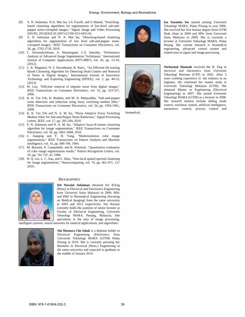
[8] S. N. Sulaiman, N.A. Mat Isa, I.A Yusoff, and F.Ahmad, "Switching-

based clustering algorithms for segmentation of low-level salt-and-

pepper noise-corrupted images," Signal, Image and Video Processing

(SIViP), 2013(DOI:10.1007/s11760-013-0455-0).

[9] S. N. Sulaiman and N. A. Mat Isa, "Denoising-based clustering

algorithms for segmentation of low level salt-and-pepper noise-

corrupted images," IEEE Transactions on Consumer Electronics, vol.

56, pp. 2702-2710, 2010.

[10] C. Sriramakrishnan, A. Shanmugam, C.S. Smruthy, "Perfomance

Analysis of Advanced Image Segmentation Techniques," International

Journal of Computer Applications (0975-8887), vol. 45, pp. 13-18,

(2012).

[11] L. K. Maguluri, N. S. Parvathanni, R. Karri,, "An Efficient De noising

Based Clustering Algorithm for Detecting Dead Centers and Removal

of Noise in Digital Images," International Journal of Innovative

Technology and Exploring Engineering (IJITEE), vol. 2, pp. 48-53,

(2013).

[12] W. Luo, "Efficient removal of impulse noise from digital images,"

IEEE Transactions on Consumer Electronics, vol. 52, pp. 523-527,

2006.

[13] K. K. Vin Toh, H. Ibrahim, and M. N. Mahyuddin, "Salt-and-pepper

noise detection and reduction using fuzzy switching median filter,"

IEEE Transactions on Consumer Electronics, vol. 54, pp. 1956-1961,

2008.

[14] K. K. Vin Toh and N. A. M. Isa, "Noise Adaptive Fuzzy Switching

Median Filter for Salt-and-Pepper Noise Reduction," Signal Processing

Letters, IEEE, vol. 17, pp. 281-284, 2010.

[15] S. N. Sulaiman and N. A. M. Isa, "Adaptive fuzzy-K-means clustering

algorithm for image segmentation," IEEE Transactions on Consumer

Electronics, vol. 56, pp. 2661-2668, 2010.

[16] L. Jianqing and Y. H. Yang, "Multiresolution color image

segmentation," IEEE Transactions on Pattern Analysis and Machine

Intelligence, vol. 16, pp. 689-700, 1994.

[17] M. Borsotti, P. Campadelli, and R. Schettini, "Quantitative evaluation

of color image segmentation results," Pattern Recognition Letters, vol.

19, pp. 741-747, 6// 1998.

[18] H. Q. Liu, L. C. Jiao, and F. Zhao, "Non-local spatial spectral clustering

for image segmentation," Neurocomputing, vol. 74, pp. 461-471, 12//

2010.

BIOGRAPHIES

Siti Noraini Sulaiman obtained her B.Eng

(Hons) in Electrical and Electronics Engineering

from Universiti Sains Malaysia in 2000, MSc

and PhD in Biomedical Engineering (focusing

on Medical Imaging) from the same university

in 2003 and 2012 respectively. Siti Noraini

currently holds the position of senior lecturer at

Faculty of Electrical Engineering, Universiti

Teknologi MARA, Penang, Malaysia. She

specializes in the area of image processing,

intelligent systems, neural networks for medical applications, and algorithms.

Siti Mastura Che Ishak is a diploma holder in

Electrical Engineering (Electronic) from

Universiti Teknologi MARA (UiTM) Pulau

Pinang in 2010. She is currently persuing her

Bachelor in Electrical (Hons.) Engineering at

the same university and expected to graduate in

the middle of January 2014.

Iza Sazanita Isa started joining Universiti

Teknologi MARA, Pulau Pinang in year 2006.

She received her first honour degree from UiTM

Shah Alam in 2004 and MSc from Universiti

Sains Malaysia in 2009. She is currently a

lecturer at Universiti Teknologi MARA, Pulau

Pinang. Her current research is biomedical

engineering, advanced control system and

related area in signal and image processing

Norhazimi Hamzah received the B. Eng in

electrical and electronics from Universiti

Teknologi Petronas (UTP) in 2002. After 3

years working experience in the industry as an

engineer, she continued her master study at

Universiti Teknologi Malaysia (UTM). She

obtained Master in Engineering (Electrical

Engineering) in 2007. She joined Universiti

Teknologi MARA (UiTM) as a lecturer in 2008.

Her research interest include sliding mode

control, nonlinear control, artificial intelligence,

automotive control, process control and

biomedical.


ISBN: 978-1-61804-232-3 39

Abstract—Conservative tillage systems, specific to sustainable

agriculture, require productivity at least equal to that of conventional technology, optimized energy efficiency and, at the same time, diminished environmental impact. An energy saving way is that of implementing optimal technology specific to each culture and pedoclimatic area. The minimum tillage and no-tillage systems represent alternatives to the conventional system of soil tillage, due to their conservation effects on soil features and to the assured productions, maize: 96-98.1% at minimum tillage and 99.8% at no-tillage, soybean: 102.9-111.9% at minimum tillage and 117.2% at no-tillage, wheat: 93.4-96.8% at minimum tillage and 106.9% at no-tillage, as compared to the conventional system. Correct choice of the right soil tillage system for the crops in rotation help reduce energy consumption, thus maize: 97.3-97.9% at minimum tillage and 91.3% at no-tillage, soybean: 98.6-98.2% at minimum tillage and 92.8% at no-tillage, wheat: 97.4-98% at minimum tillage and 91.6% at no-tillage. Energy efficiency is in relation to reductions in energy savings, but also with efficiency and impact on the tillage system on the cultivated plant. For all crops in rotation, energy efficiency (energy produced from 1 MJ consumed) was the best in no-tillage and 10.44 MJ ha-1 at maize, 6.49 MJ ha-1 at soybean, 5.66 MJ ha-1 at wheat. Energy-efficient agricultural system: the energy consumed-energy produced-energy yield, necessarily have to be supplemented by soil energy efficiency, with the conservative effect of the agricultural system. Only then the agricultural system will be sustainable, durable in agronomic, economic and ecological terms. The implementation of minimum and no-tillage soil systems have increased the organic matter content from 2 to 7.6% and water stabile aggregate content from 5.6 to 9.6%, at 0-30 cm depth, as compared to the conventional system. While the soil fertility and the wet aggregate stability have initially been low, the effect of conservation practices on the soil characteristics led to a positive impact on the water permeability in the soil. Availability of soil moisture during the crop growth led to a better plant watering condition. Subsequent release of conserved soil water regulated proper plant water condition and soil structure.

Keywords—No-tillage, minimum tillage, yield, energy efficiency, soil conservation.

I. INTRODUCTION USTAINABLE agricultural activity must be organized in a system, scheduled in a sequence and always analysed as part of the relationship: soil-plant-climate area-socio-

economic conditions-crop-efficiency [1], [4], [6], [24]. Recommendation of flexible and multifunctional technologies

Rusu, T. is a Professor of Agrotechnics in the University of Agricultural Sciences and Veterinary Medicine Cluj, 3-5 Manastur Street, Cluj-Napoca, 400372, Romania (phone: 0040724719774; fax: 0040264593792; e-mail: [email protected]).

consequently equally aims at reducing the consumption of energy, particularly in the field of aggressive soil tillage, as well as obtaining high yields, soil conservation and environmental protection [2], [8], [11], [13].

The essence of the living system consists in the unique capacity of plants to convert, through photosynthesis, the solar energy, carbon dioxide and water into biochemical alimentary energy. Therefore, a successful measure in agriculture is the quantity of energy gathered under the form of biomass, as a result of efficient human and fossil energy use [3], [5], [9], [10], [12].

The soil tillage has as main purpose a series of immediate effects (with a positive side), resulting from the objectives of the soil tillage themselves: basic tillage, germinal layer preparation, field maintenance. Still, the effects of the soil tillage can often have an immediate negative part or long lasting effects, positive or negative [13], [15], [16], [19], [23], [26], [30].

The influence of soil tillage system on soil properties and energy efficiency is proved by important factors of soil fertility conservation and evaluation of the sustainability of agricultural system [21], [25], [28], [29]. Long-term field experiments provide excellent opportunities to quantify the long-term effects of soil tillage systems on accumulated soil water [18], [20], [22]. The hydrological function of the soil (especially the capacity to retain optimum water quantity, and then gradually make this available for plant consumption) is one of the most important functions determining soil fertility, productivity and soil evolution. Intrinsic soil properties such as organic matter and texture, along with applied tillage practices combine to modify the soil structure, porosity, permeability and water capacity. This, in turn, is a critical factor in the water cycle and affects water accumulation in the soil. The conservation of soil fertility requires a tillage system that optimizes the plant needs in accordance with the soil modifications, that ensures the improvement of soil features and obtaining large and constant crops. Thus, the conservation of soil fertility is tied to maintaining and improving the soil fertility indices and to the productivity of the tillage system.

II. MATERIALS AND METHODS The experiments have been conducted at the University of

Agricultural Sciences and Veterinary Medicine in Cluj Napoca, Romania (46º46'N, 26º36'E), on a moderately fertile Fluvisoil [32]. The humus content was 3.01%, pH was 7.2, and soil texture was clay (42% clay in the arable stratum). The

Energy Efficiency of Conservative Tillage Systems in the Hilly Areas of Romania

Rusu Teodor

S


ISBN: 978-1-61804-232-3 40

experimental field has an annual temperature of 8.20C and annual rainfall of 613 mm.

Treatments used in the study were as follows: A. Conventional tillage (CT): V1-classic plough (20-25 cm) + disc harrow-2x (8 cm) (witness treatment). B. Minimum tillage (MT): V2-paraplow (18-22 cm) + rotary harrow (8 cm); V3-chisel plough (18-22 cm) + rotary harrow (8 cm); V4-rotary harrow (10-12 cm). C. No-tillage (NT): V5-direct drill with Accord Optima HD for hoeing and SUP adapted for wheat.

All soil tillage was accomplished during the autumn period for wheat; for corn and soybeans we used the plough, paraplow, chisel plough in the autumn and finally, for the germinal layer preparation, we used the disc harrow and rotary harrow in the spring. Crop rotation was: maize-Zea mays L., soy-bean-Glycine hispida L. Merr. and wheat-Triticum aestivum L.

The experimental design was a randomized complete block design with three replications. The area of a parcel was 300 m2. Except for the soil tillage system, all other variables were held constant, including the herbicide used: wheat-post emergent dicamba 120 g/l + 2.4D 300 g/l, 0.9 l ha-1; corn-pre emergent acetochlor 820-860 g/l + antidote, 2.5 l ha-1 and post emergent dicamba 120 g/l + 2.4D 300 g/l, 0.9 l ha-1; soybeans-pre emergent acetochlor 820-860 g/l + antidote, 2.5 l ha-1 and post emergent bentazon 480 g/l + Wettol 150 g/l, 2.5 l ha-1.

To quantify the change in soil properties under different tillage practices, determinations were made for each culture in four vegetative stages (spring, 5-6 leaves, bean forming and harvest). Soil parameters monitored included soil water content (gravimetric method, Aquaterr probe-Frequency domain reflectometry), soil bulk density (determined by volumetric ring method using the volume of a ring 100 cm3), water stable aggregates (Czeratzki method), soil permeability (using the Infiltrometer method) and organic matter content (Walkley-Black method). The average values obtained during the vegetal phases were statistically analysed. The results were analysed using ANOVA and Duncan's test [31]. A significance level of P ≤ 0.05 was established a priori.

Regarding energetic assessment, the most realistic means of comparison of various agricultural technologies remains energy efficiency, using the following indicators: Energy Efficiency Factor: e = (Er-Ec)/Er [MJ]; Energy Yield: γ = Er/Ec [MJ]; Energy Report r = Ec/Er [MJ]. Where: Er-energy as gathered biomass [MJ]; Ec-technologically consumed energy to produce this biomass [MJ].

Consumed and produced energy represent in fact a sum of inputs and outputs in the technological process. Consequently: Er = Erp+Ers [MJ]. Where: Erp-energy corresponding to primary harvest; Ers-energy corresponding to secondary harvest.

Technologically consumed energy has several components: Ec=Ect+Ecm+Ecs+Ecf+Ecp+Ecu+Eo [MJ]. Where: Ect-energy consumption related with the tractor [MJ]; Ecm-energy consumption related with agricultural machinery [MJ]; Ecs-energy consumption related with seeds [MJ]; Ecf-energy consumption related with fertilization [MJ]; Ecp-energy consumption related with pesticides [MJ]; Ecu-energy consumption related to human work resources [MJ]; Eo-

energy consumed in other ways [MJ]. Each component is the sum of elementary energies specific to each technological operation. Quantification of consumed energy and of the produced energy has been achieved on the basis of equivalents mentioned in specialty literature [7], [17], [27].

The equivalence indicators are: Energy consumed: basic tillage-classic plow: 1,102.98 MJ

ha-1; paraplow: 853.92 MJ ha-1; chisel: 782.76 MJ ha-1; rotary grape: 711.6 MJ ha-1; direct sowing: 978.24 MJ ha-1. Preparation of the germinative layer-disc: 426.96 MJ ha-1; rotary grape: 640.44 MJ ha-1. Fertilization-135.97 MJ ha-1. Materials-1 kg N: 92.51 MJ; 1 kg P2O5: 20.34 MJ; 1 kg K2O: 14.84 MJ; 1 l diesel oil: 35.58 MJ; 1 kg bentazone: 252.5 MJ; 1 kg acetochlorine: 101.3 MJ; 1 kg dicamba: 294 MJ; 1 kg insecticide, fungicide: 205.2 MJ. Sowing-corn: 160.11 MJ ha-

1; soy bean: 160.11 MJ ha-1; wheat: 192.13 MJ/ha. Herbicides: 46.25 MJ/ha. Harvest: 511.99 MJ ha-1. Human work force: 1.318 MJ/person/hour. Other energetic inputs: 426.96 MJ ha-1.

Energy produced-1 kg corn: 16.41 MJ; 1 kg corn cob: 15.29 MJ; 1 kg soy bean: 20.79 MJ; 1 kg soy stems: 15.42 MJ; 1 kg wheat: 16.06 MJ; 1 kg wheat straws: 15.26 MJ.

III. RESULTS AND DISCUSSION The soil tillage system influences the yields obtained in a

differentiated way, depending on the culture type (table 1). Corn crop assures the highest yield with plough and no-tillage systems. Paraplow and chisel give smaller yields (6,710-6,730 kg ha-1), with statistically ensured differences (significantly negative) and confirmed by the test of multiple comparisons, Duncan's test (ab). The smallest corn productions were obtained with rotary harrow, the differences being distinctly negative, statistically ensured (b). Soybean culture had the best reaction within the rotation, both with the no-tillage (very significant positive differences as compared to the plough), as well as with minimum soil tillage system, with paraplow and rotary harrows (ab). For wheat culture no-tillage ensure highest yield, 3,986 kg ha-1, and the lowest production has been achieved with chisel (93.4%).

The quantity of energy produced depending on soil tillage system, is related to main and secondary yield, being higher in the plough variant. Energy efficiency is influenced by the soil tillage system, being higher in no-tillage (e=0.9042, 101%), followed by the variants with chisel and paraplow (100.1%). Energetic efficiency is influenced by the energy consumed within every technologic system, the smaller the consumed energy within the system, the higher the efficiency. The high power efficiency in no-tillage (γ=10.44 MJ ha-1), chisel (γ =9.66 MJ ha-1) and paraplow (γ =9.65 MJ ha-1), as compared to the plough system (γ =9.54 MJ ha-1), shows that the energy invested in these variants has had a higher efficiency. The proportional expression between the produced and consumed energy, through energetic report, as certains the lower value of this indicator of 0.096 in no-tillage and the highest value, of 0.108 for the rotary harrow variant.

Considering the amount of produced energy, in maize culture, we can emphasize the advantages of the plough variant. The intense soil mobilization, in conjunction with the effects produced in the soil linked to the release of adequate


ISBN: 978-1-61804-232-3 41

nutrients and providing necessary conditions for maize development ensures the highest productions. Intense impact on soil does not, however, always have positive effects. Eventually, the energy efficiency demonstrates the superiority

of the no-tillage and minimum tillage systems, in terms of energy consumption reductions and optimization of agricultural technologic system.

Table 1. The influence of different soil tillage systems upon the plants yield in the case of maize, soybean and wheat crops.

Soil tillage systems Classic plough + disc-2x

Paraplow + rotary harrow

Chisel plow + rotary harrow Rotary harrow No Tillage

Maize, kg ha-1 6,860 a 6,730 ab 6,710 ab 6,583 b 6,849 a Significance (%) wt.(100) 0(98.1) 0(97.8) 00(96) ns(99.8) Soybean, kg ha-1 3,025 b 3,385 ab 3,113 b 3,313 ab 3,546 a Significance (%) wt.(100) **(111.9) ns(102.9) **(109.5) ***(117.2) Wheat, kg ha-1 3,730 ab 3,615 ab 3,486 b 3,612 ab 3,986 a Significance (%) wt.(100) ns(96.9) 0(93.4) ns(96.8) *(106.9)

Note: wt-witness, ns-not significant, *positive significance, 0negative significance, a, ab, b, c-Duncan’s classification (the same letter within a row indicates that the means are not significantly different) Maize: DL5% = 100.01 kg ha-1, DL1% = 151.45 kg ha-1, DL0.1%= 243.30 kg ha-1 Soybean: DL5% = 190.75 kg ha-1, DL1% = 271.16 kg ha-1, DL0.1%= 392.62 kg ha-1 Wheat: DL5% = 241.21 kg ha-1, DL1% = 338.57 kg ha-1, DL0.1%=477.99 kg ha-1

Table 2. The influence of the soil tillage system on energy efficiency in maize culture. Variant Energy, MJ Energy Efficiency Energy yield

(γ) Energy

report (r) Consumption (%) Produced e % Classic plough + disc-2x (wt) 22,364.09 (100) 213,417.78 0.8952 100 9.54 0.104 Paraplow + rotary harrow 21,901.55 (97.9) 211,284.48 0.8963 100.1 9.65 0.103 Chisel plow + rotary harrow 21,830.39 (97.6) 210,956.28 0.8965 100.1 9.66 0.103 Rotary harrow 21,759.23 (97.3) 200,646.19 0.8915 99.6 9.22 0.108 No-Tillage 20,425.41 (91.3) 213,237.27 0.9042 101.0 10.44 0.096

The energy required for setting up and maintaining the

soybean culture after conventional system represents 25,364.09 MJ/ha and goes down to 97.6-98.2% at MT and at 92.8% at NT. Energy efficiency is superior in all variants as

compared to the witness, soy reacting very well with MT and NT systems. Energy yield confirms this positive reaction, the results being 6.49 MJ ha-1 at NT and 5.51-5.97 MJ ha-1 at MT, for 1 MJ ha-1 consumed.

Table 3. Influence of soil tillage system on energy efficiency in soybean culture.

Variant Energy, MJ Energy Efficiency Energy Yield (γ)

Energy report (r) Consumption (%) Produced e %

Classic plough + disc-2x (wt) 25,364.09 (100) 132,858.00 0.8091 100 5.23 0.191 Paraplow + rotary harrow 24,901.55 (98.2) 148,669.20 0.8325 102.9 5.97 0.167 Chisel plow + rotary harrow 24,830.39 (97.9) 136,722.98 0.8184 101.1 5.51 0.182 Rotary harrow 24,759.23 (97.6) 145,506.96 0.8298 102.5 5.88 0.170 No-Tillage 23,545.75 (92.8) 152,740.32 0.8458 104.5 6.49 0.154

In the case of autumn wheat culture, technology is

energetically equivalent to 23,272.38 MJ ha-1 through the CT system (table 4). Application of MT reduces energy consumption to 97.4-98%, and NT to 91.6%, compared with the plough system. The influence of the soil tillage system on the amount of gathered energy reflects on the energy efficiency factor, where, in comparison with the witness, a higher efficiency at NT has been calculated (101%). Energy efficiency has been reduced in the other variants, but it does not fall below 99%. Energy yield shows that in 1 MJ ha-1

consumed a larger amount of energy is obtained with no-tillage (γ=5.66 MJ ha-1), and the lowest yield was recorded with the chisel plough variant, 5.32 MJ ha-1. The energy report has the best value in no-tillage (0.177), followed by the plough variant (0.179).

Statistical analysis of the results demonstrated that the differences in accumulated soil water depended on the variants of soil tillage (table 5). Soil texture and structure have a strong effect on the available water capacity. The results clearly demonstrate that MT and NT systems promote increased humus content (2-7.6%) and increased water constant aggregate content (5.6-9.6%) at 0-30 cm depth as compared to conventional tillage. Multiple analysis of soil classification and tillage system on the hydric stability of soil structure and water supply accumulated in soil have shown that all variants with minimum tillage are superior (b, c), having a positive influence on soil structure stability. The increase in organic matter content is due to the vegetal remnants at the soil surface (NT) or partially incorporated (MT) and adequate biological activity in this system. In the case of humus content and also in the


ISBN: 978-1-61804-232-3 42

hydro stability structure, the statistical interpretation of the data shows an increasing positive significance of the MT and NT systems application. The soil fertility and wet aggregate stability were initially low, the effect being the conservation of the soil features and also their reconstruction, with a positive influence on the permeability of the soil for water. More aggregated soils permit more water to reach the root zone. This does not only increase productivity, but it also reduces runoff, and thus the erodibility potential.

The bulk density values at 0-30 cm increased by 0.01-0.03% under minimum and no-tillage systems. This raise was not significant in any of the experimental variants. Multiple comparing and classification of experimental variants align all values on the same level of significance (a). On molic Fluvisoils, soils with good permeability, high fertility, and low susceptibility to compaction, accumulated water supply was higher (representing 12.4-15%) for all minimum and no-tillage soil systems.

Table 4. Influence of soil tillage system on energy efficiency in wheat culture.

Variant Energy, MJ Energy efficiency Energy yield (γ)

Energy report (r) Consumption (%) Produced e %

Classic plough + disc-2x (wt) 23,272.38 (100) 129,458.88 0.8202 100 5.56 0.179 Paraplow + rotary harrow 22,809.84 (98.0) 125,475.58 0.8182 99.7 5.50 0.182 Chisel plow + rotary harrow 22,738.68 (97.7) 120,992.76 0.8121 99.0 5.32 0.188 Rotary harrow 22,667.52 (97.4) 125,366.36 0.8192 99.9 5.53 0.181 No-Tillage 21,315.48 (91.6) 120,586.40 0.8232 100.4 5.66 0.177

Table 5. The influence of soil tillage system upon soil properties (0-30 cm).

Soil tillage systems Classic plough + disc –2x (wt)

Paraplow + rotary harrow

Chisel plow + rotary harrow Rotary harrow No-tillage

OM, % 3.03 a 3.12 ab 3.09 ab 3.23 b 3.26 b Significance (%) wt.(100) ns(103.1) ns(102.0) ns(106.5) ns(107.6) WSA, % 71.33 a 76.00 b 75.33 b 76.33 b 78.21 b Signification (%) wt. (100) * (106.5) *(105.6) *(107.0) *(109.6) BD, g/cm3 1.34 a 1.34 a 1.35 a 1.34 a 1.38 a Signification (%) wt..(100) ns(100.0) ns(100.6) ns(100.0) ns(102.9) W, m3/ha 878 a 1.010 c 998 b 987 b 995 b Signification (%) wt..(100) *(115.0) *(113.7) *(112.4) *(113.3)

Note: wt-witness, ns-not significant, *positive significance, 0negative significance, a, ab, b, c-Duncan’s classification (the same letter within a row indicates that the means are not significantly different). OM-organic matter. WSA-water stability of structural macro-aggregates. BD-bulk density. W-water supply accumulated in soil.

IV. CONCLUSIONS The minimum tillage and no-tillage systems represent

alternatives to the conventional system of soil tillage, due to their conservation effects on soil features and to the assured productions, maize: 96-98.1% at MT and 99.8% at NT, soybean: 102.9-111.9% at MT and 117.2% at NT, wheat: 93.4-96.8% at MT and 106.9% at NT, as compared to the conventional system.

Correct choice of the right soil tillage system for the crops in rotation help reduce energy consumption, thus maize: 97.3-97.9% at MT and 91.3% at NT, soybean: 98.6-98.2% at MT and 92.8% at NT, wheat: 97.4-98% at MT and 91.6% at NT. Energy efficiency is in relation to reductions in energy savings, but also with efficiency and impact on the tillage system on the cultivated plant, maize: 99.6-100.1% at MT and 101% at NT, soybean: 101.1-102.9% at MT and 104.5% at NT, wheat: 99-99.9% at MT and 100.4% at NT. For all crops in rotation, energy efficiency (energy produced from 1 MJ consumed) was the best in no-tillage and 10.44 MJ ha-1 at maize, 6.49 MJ ha-1

at soybean, 5.66 MJ ha-1 at wheat. Energy-efficient agricultural system: the energy consumed-

energy produced-energy yield, necessarily have to be supplemented by soil energy efficiency, with the conservative effect of the agricultural system. Only then the agricultural

system will be sustainable, durable in agronomic, economic and ecological terms.

This study demonstrated that increased organic matter content in soil, aggregation, and permeability are all promoted by minimum and no-tillage systems. The implementation of such practices ensures a greater water supply. The practice of reduced tillage is ideal for enhancing soil fertility, water accumulation capacity, and reducing erosion. The advantages of minimum and no-tillage soil systems for Romanian pedoclimatic conditions can be used to improve methods in low producing soils with reduced structural stability on sloped fields, as well as measures of water and soil conservation on the whole ecosystem.

REFERENCES [1] Afzalinia, S., A. Khosravani, A. Javadi, D. Mohammadi and

Alavimanesh, S. M. 2012. Effect of Tillage and Planting Methods on the Soil Properties, Grain Drill Performance, and Wheat Yield. Journal of Agricultural Science and Technology A2, 537-543.

[2] Ailincai, C., G. Jitareanu, D. Bucur and Mercus, A. 2011. Influence of tillage practices and fertilization on crop yields and soil properties in long-term crop rotation (soybean-wheat-maize) experiments. Journal of Food, Agriculture & Environment, Vol. 9 (1), 285-289.

[3] Akdemir, S., H. Akcaoz and Kizilay, H. 2012. An analysis of energy use and input costs for apple production in Turkey. Journal of Food, Agriculture & Environment Vol. 10 (2), 473-479.


ISBN: 978-1-61804-232-3 43

[4] Bucur, D., G. Jitareanu and Ailincai, C. 2011. Effects of long-term soil and crop management on the yield and on the fertility of eroded soil. Journal of Food, Agriculture & Environment Vol.9 (2), 207-209.

[5] Coman, M. and Rusu, T. 2010. New ways in using far-infrared radiations for agricultural production. Journal of Food, Agriculture & Environment Vol. 8, No. 3-4, 714-716.

[6] Domuta, C., M. Sandor, Gh. Ciobanu, A. Samuel, C. Ciobanu, A. Domuta, C. Borza, Cr. Domuta, R. Brejea and Gatea, M. 2012. Influence of the crop system on soil erosion and on the soil physical properties under the Romanian north-western area conditions. Journal of Environmental Protection and Ecology 13 (2), 736-745.

[7] Fluck, R.C. and Baird C.D. 1980. Agricultural energetics. AVI Publishing Co., Westport, Connecticut.

[8] Gao, S., X. Tong and Wu, L. 2012. Environmental constraints and transformation of China's export structure. Journal of Food, Agriculture and Environment 10 (1), 919-922.

[9] Glendining, M. J., A. G. Dailey, A. G. Williams, F. K. van Evert, K.W.T. Goulding and Whitmore, A. P. 2009. Is it possible to increase the sustainability of arable and ruminant agriculture by reducing inputs?. Agricultural Systems, Vol. 99, Issues 2–3, 117-125.

[10] Jackson, T. M., M. A. Hanjra, S. Khan and Hafeez, M. M. 2011. Building a climate resilient farm: A risk based approach for understanding water, energy and emissions in irrigated agriculture. Agricultural Systems, Vol. 104, Issue 9, 729-745.

[11] Jitareanu, G., C. Ailincai and Bucur, D. 2006. Influence of Tillage Systems on Soil Physical and Chemical Characteristics and Yield in Soybean and Maize Grown in the Moldavian Plain (North – Eastern Romania), p. 370-379. In International Symposium, Soil Management for Sustainability, Adavances in GeoEcology 38, Catena Verlag Ed., Germany.

[12] Jones, M. R. 1989. Analysis of the use of energy in agriculture - Approaches and problems. Agricultural Systems, Vol. 29, Issue 4, 339-355.

[13] Marin, D.I., M. Mihalache, C. Ciontu, C. Bolohan and Ilie, L. 2011. Influence of soil tillage of pea, wheat and maize crop in the Moara Domneasca-Ilfov area. 5th International Symposium - Soil Minimum Tillage System, p. 111-118, Ed. Risoprint Cluj-Napoca.

[14] Marin, D. I., T. Rusu, M. Mihalache, L. Ilie and Bolohan, C. 2012. Research on the influence of soil tillage system upon pea crop and some properties of reddish preluvosoil in the Moara Domneasca area. Annals of the University of Craiova – Agriculture, Montanology, Cadastre Series, Vol. 42, No. 2, 487-490.

[15] Molnar, A., I. Drocas, O. Ranta and Stanila, S. 2012. Development of Software for Soil Compaction Assessment. Bulletin UASVM Agriculture, 69(1-2)/2012.

[16] Moraru, P. I. and Rusu, T. 2012. Effect of tillage systems on soil moisture, soil temperature, soil respiration and production of wheat, maize and soybean crops. Journal of Food, Agriculture & Environment, Vol. 10, Issue 2, 445-448.

[17] Pimentel, D. 1992. Energy inputs in agriculture production. In Fluck, R. C. (ed.). Energy in World Agriculture. Vol. 6. Elsevier Sci. Publ. Co., Amsterdam, pp. 13-29.

[18] Ponjican, O. O., A. M. Bajkin, G. P. Jacimovic, M. D. Tomic, L. D. Savin, N. M. Dedovic and Simikic, M. D. 2012. Tillage quality affecting physical characteristics, number of plants and carrot root yield under flat and ridge cultivation. Journal of Food, Agriculture & Environment Vol.10 (2): 304-311.

[19] Ranta, O., I. Drocas, S. Stanila, A. Molnar, M.V. Muntean and Marian, O. 2012. Analysis of Working Qualitative Parameters for No-Till Machines. Bulletin UASVM Agriculture, 68(1)/2011.

[20] Romaneckas, K., V. Pilipavicius, E. Sarauskis and Sakalauskas, A. 2009. Effect of sowing depth on emergence and crop establishment of sugar beet (Beta vulgaris L.). Journal of Food, Agriculture & Environment, 7 (2), 571-575.

[21] Rusu, T. 2001. The influence of Minimum Soil Tillage upon the soil, yield and efficiency. PhD Thesis, University of Agricultural Sciences and Veterinary Medicine of Cluj-Napoca, Romania.

[22] Rusu, T., P. Gus and Bogdan, I. 2006. The influence of minimum soil tillage systems on weed density, frequency of phytopatogenous agents and crop yields of soybean, wheat, potato, rape and corn. Journal of Food, Agriculture & Environment, Vol. 4, No. 1, 225-227.

[23] Rusu, T. and Bogdan, I. 2012. Influence of Degree Infestation with Echinochloa crus–galli Species on Crop Production in Corn. In Herbicides - Properties, Synthesis and Control of Weeds, Mohammed Naguib Abd El-Ghany Hasaneen (Ed.), InTech Ed.

[24] Sadegh, A., A. Khosravani, A. Javadi, D. Mohammadi and Alavimanesh, S.M. 2012. Effect of Tillage and Planting Methods on the Soil Properties, Grain Drill Performance and Wheat Yield. Journal of Agricultural Science and Technology A 2, 537-543.

[25] Sarauskis, E., E. Vaiciukevicius, K. Romaneckas, A. Sakalauskas and Baranauskaite, R. 2009b. Economic and energetic evaluation of sustainable tillage and cereal sowing technologies in Lithuania. Rural Development 4(1), 280-285.

[26] Stanila, S., I. Drocas, O. Ranta, A. Molnar and Nagy, M. 2012. Studies regarding comparative analysis of main working indicators at primary soil tillage's. Bulletin UASVM Agriculture, 69(1-2)/2012.

[27] Tesu, I. and Baghinschi, V. 1984. Energy and Agriculture. Methodology for calculation and analysis of energy efficiency in Agriculture. Ceres Ed., Bucharest, Romania.

[28] Uhlin, H. E. 1998. Why energy productivity is increasing: An I-O analysis of Swedish agriculture. Agricultural Systems, Vol. 56, Issue 4, 443-465.

[29] Vural, H. and Efecan, I., 2012. An analysis of energy use and input costs for maize production in Turkey. Journal of Food, Agriculture & Environment Vol.10 (2): 613-616.

[30] Zhou, X.M., Z.F. Zuo and Liu, B. 2012. The dynamic distribution of Mn element between soil and plant in Northeast Leymus chinensis grassland. Journal of Food Agriculture & Environment, Vol. 10 No. 2, 891-895.

[31] PoliFact, 2010. ANOVA and Duncan's test pc program for variant analyses made for completely randomized polifactorial experiences. USAMV Cluj-Napoca, Romania.

[32] SRTS, 2003. Romanian System of Soil Taxonomy. Estfalia Ed., Bucharest, Romania.


ISBN: 978-1-61804-232-3 44

http://www.isfae.org/scientficjournal/2012/issue2/pdf/agriculture/a26.pdf



Abstract—This paper illustrates a new multidirectional method for

assessing cliff instability susceptibility at a given scale (CISA, Cliff Instability Susceptibility Assessment) through a case study along the Murgia coastline North of Bari (Apulia, SE Italy). The stretch of coastline considered in this study shows an indented rocky coast with cliffs up to 12 m high, numerous small to medium-sized caps and inlets, and a well protected tourist port. The coastal outcrops are made up of Mesozoic carbonate rocks which are thickly-bedded (0.2-1.0 m) and, moderately to highly fractured and karstified. At places, clear signs of coastal erosion are evident; they consist mainly of rock falls caused by differential erosion of rock strata of varying resistance to weathering and sea wave action on the cliff face. The CISA method is based on classifying coastal sectors using above all morphological criteria and characterising them estimating and combining 28 incidence parameters according to an heuristic approach. These parameters were divided in four categories: geomechanical (12), morphological (6), meteo-marine (8) and anthropogenic (2). For each parameter 5 classes of rating were proposed; the cliff classification, in terms of cliff instability susceptibility, was obtain from the total rating which represents the summation of the single rating of the individual parameter.

Keywords—Cliff, Carbonate, Instability, Method.

I. INTRODUCTION N many sites of Apulia (SE Italy), the coastline is gradually receding inland as a result of natural and human processes. In particular, morphologic features of the rocky coast,

mostly produced by Quaternary tectonics, are strongly conditioned by complex mechanisms involving sea waves action against the cliffs, carbonation, weathering and urbanization pressure [1]. The dominant and more visible retreat process of the cliffs consists of slope mass movements of different types and sizes, which include rockfalls, topples and slides controlling by discontinuity pattern and density, and mechanical properties of the carbonate outcrops. Actually, many are the basic factors which play an important role in the

This work was supported in part by MIUR (Italian Ministry of Education, University and Research) under Grant 2010 ex MURST 60% “Modelli geologico-tecnici, idrogeologici e geofisici per la tutela e la valorizzazione delle risorse naturali, ambientali e culturali” (Resp.: Gioacchino Francesco Andriani).

G. F. Andriani is with the Department of Earth and Geoenvironmental Science, University of Bari Aldo Moro, BA 70125 ITALY (corresponding author, phone: +39-080-5442572; fax: +39-080-5442625; e-mail: [email protected]).

V. Pellegrini is a free researcher at the Department of Earth and Geoenvironmental Science, University of Bari Aldo Moro, BA 70125 ITALY (e-mail: [email protected]).

assessment of the retreat mechanisms of the Apulian rocky cliffs and the mapping of the coastal stretches most susceptible to erosion is not a simple matter. Different methods are adopted for determining potentially instable areas or landslide hazard assessments; these techniques can be divided into three groups: expert evaluation, statistical methods, and mechanical approach [2]-[3]-[4]-[5] and references therein.

Fig.1. Geographic location of the study area.

Thus, considering advantages and disadvantages

of these approaches and the complexity of this problem as well as its economical aspect, a new multidirectional method is proposed in this paper for assessing cliff instability susceptibility at a given scale (CISA, Cliff Instability Susceptibility Assessment). In order to highlight the role and relationships of factors and eroding processes affecting the morphodynamic evolution of rocky coasts in a typical Mediterranean coastal carbonate environment, a case study along a stretch of coastline of approximately 2000 m in the territory of Giovinazzo, about 20 km NW of Bari, is carried out. The suggested method is based on the expert evaluation approach and is calibrated by morphological analysis, morphoevolutive models, geomechanical surveys, geotechnical laboratory tests, deterministic analysis (the estimate of the critical height for vertical cliffs using the lower bound theorem of limit analysis) and completed by GIS-based stability assessment and mapping.

II. SETTING The study area is located on the Adriatic side of the Murge

plateau, an emerged part of the Apulian foreland, about 20 km NW of Bari, in the territory of the Municipality of Giovinazzo (Fig. 1). The Murge plateau is characterized by a 3 km thick

A suggested method for assessing cliff instability susceptibility at a given scale (CISA)

G.F. Andriani, V. Pellegrini

I


ISBN: 978-1-61804-232-3 45

Cretaceous shallow-water succession of limestones and dolostones forming a S-SW dipping monocline slightly deformed by folds and sub-vertical normal and transtensional faults [6]. This succession consists of lagoonal and peridital carbonates mostly deposited in low-energy inner-platform environments [7]. Only few stratigraphic intervals contain more open- and deeper-marine lithofacies in which abundant and diversified associations of rudists and benthic foraminifera can be found [8]. The limestones and dolostones are bedded, jointed and subjected to karst processes, and represent a peculiar hydrogeological domain. In fact, the hydraulic base level of groundwater circulation corresponds to sea level. Several coastal springs drain groundwater along preferential pathflows where rock-mass permeability is greater [1]. The prevailing morphologic characteristic of the Apulian coastal area is the presence of a series of marine terraces linked by small scarps subparallel to the coastline. These are carved by short erosive incisions (locally named “lame” and “gravine”) in simple catchments and watersheds that are difficult to recognize, as often occurs in karst areas [9]-[10]. The marine terraces develop on wide plains from about 150 m a.s.l. to the present sea level, maintaining a gentle slope to the NE, and give the southeastern side of the Murge a typical terraced profile.

Fig. 2 - Appearance of the rock mass exposed along the

coastal stretch of Giovinazzo. The coastal stretch of Giovinazzo is characterized by the

outcropping of the lower part of the Calcare di Bari Fm. (Callovian pp.-early Turonian). This part consists of an about 25-m-thick interval characterized by rudist-dominated medium- to coarse-grained deposits. Rudists form dm- to m-thick sheetlike tabular bodies with whole shells in growth position or more commonly randomly oriented [7]-[8]. The rudist beds gradually pass upward to mud-dominated fine-grained biopeloidal mudstones/wackestones and to laminated fenestral peloidal bindstone showing microbial laminations (Fig. 2).

Morphological features along the Giovinazzo shoreline are typical of an indented rocky coastline where caps and inlets

follow each other and steep cliffs, here from about 1.0 m (microcliffs) to 10 m in height, end in subhorizontal surfaces at the top and bottom. Before the tourist port, further to NW, the cliff is protected by a subhorizontal or gently sloping inward wave-cut platform; the last extends from the base of the cliff for 5 m to 10 m and is submerged or emerged with rising and falling of the sea level. The most part of the coastal stretch is protected by a retaining wall made of carbonate stone masonry or unreinforced concrete (Fig. 3).

Fig. 3 - Retaining wall made of carbonate stone masonry along

the coastline of Giovinazzo. The wall is about 12 m at its highest part where there is the

south side of the historical center of the city which lies on a promontory overlooking the sea. The north side of the historical center overlooks the tourist port which is bordered seaward by two jetties. Large rock or concrete boulders chaotically arranged were used in the past for the protection of the cliff and the outer walls of the old city (Fig. 4).

Fig. 4 – Large square boulders used for the protection of the

old city.

To the SE, a bay characterized the whole sector that at


ISBN: 978-1-61804-232-3 46

places presents a small beach mainly formed by calcareous and concrete pebbles coming from coastal erosion processes and improvised attempts of beach nourishment (Fig. 5).

Fig. 5 – Small beach mainly formed by calcareous and

concrete pebbles.

III. METHOD The CISA method (Cliff Instability Susceptibility

Assessment) is a multidirectional method for assessing cliff instability at a given scale. The first step of the method consists of the subdivision of the coastal stretch in coastal sectors based above all on morphological criteria. Cliff height, coastal landforms (caps, inlet etc.), wave and wind exposure, coastal defence structures, natural and artificial in types (wave-cut platform, beach, rock blocks, jetties etc.), were taken into account to subdivide in 5 sectors the coastal stretch under consideration. “Regional Technical Map” (CTR) of Apulia at scale 1:5000 (www.sit.puglia.it), georeferented to WGS84/UTM zone 33N system, was used as base map to generate the Coastal Stability Map of the study area (Fig. 6).

Fig. 6 – Costal stability map of the study area.

In the second phase, a qualitative assessment of the cliff

stability integrating traditional geomechanical surveys was completed by geotechnical laboratory tests, deterministic analysis (the estimate of the critical height for vertical slope using the lower bound theorem of limit analysis), multifactor spatial GIS analysis using physical geographically-based measures with the purpose of assigning the right weight

to the parameters considered in this study. 28 incidence parameters were considered and regrouped in four categories: geomechanical (12), morphological (6), meteo-marine (8) and anthropogenic (2). For each parameter 5 classes of rating were proposed; the cliff classification, in terms of instability susceptibility, was obtain from the total rating which represents the summation of the single rating of the individual parameter (Table I). The stability classes with respect to coastal erosion are reported in Table II.

Table I – Rating of 28 parameters of the CISA method.

Table II – Stability classes as per CISA values.

Discontinuities in rock masses were described according to the ISRM standards [11]. Favorability/unfavorability of discontinuities related to cliff stability was evaluated on the basis of the ratio between discontinuity orientation and persistence, and potential failure mechanism. With respect to parallelism between joints and slope face strikes, the presence of tension cracks at the cliff-top edge was considered the most hazardous condition. The RQD estimation was carried out by the the volumetric joint count (Jv) and block sizes [12]. Notches and karst features were account as prominent natural coastal hazards. Following the standard test procedure outlined in ISRM [13]-[14], dry unit weight (γd), porosity (n) and uniaxial compressive strength in the dry state (σc) were determined on 10 cylindrical specimens (100 mm in diameter) prepared from little rock blocks fallen from the cliff face and collected along the coastline. As regards the specific gravity (G), reference was made to a value of 2.70 on the basis of the


ISBN: 978-1-61804-232-3 47

http://www.sit.puglia.it/

chemical composition of the rocks. These last, in fact, are composed mostly of carbonate with an negligible insoluble residue [15]. Dry unit weight is in the range 19.0-23.2 kN/m3, porosity between 12.2-18.1% and uniaxial compressive strength between 18.3-112.5 MPa. Rock mass hardness was measured in situ with the Schmidt hammer (type L). Higher porosity and, lower strength and density values are due to high weathering rates of a coarse-grained bed at the base of the cliff cropping out in the first coastal sector. It should be noted that in this paper the term weathering includes carbonation. For each coastal sector, the estimate of the critical height of the cliff was carried out with the lower bound theorem of limit analysis adopting the Mohr-Coulomb failure criterion. The shear strength of the rock masses was obtained with the envelope derived by [16]. A precautionary approach was adopted in the analysis so that for each lithotechnical unit estimated on the cliff the lowest value of strength was utilised. Two-dimensional cliff stability analysis was performed using the weighted mean for the geotechnical parameters of the different lithotechnical units defined on the cliff face; therefore in the vertical cliff model, shear strength and unit weight were considered as uniformly constant. A correction factor equal to RQD was applied at the weighted mean of the unit weight determined in laboratory on cylindrical samples for assessing the unit weight of the rock mass. For the submerged portion of the cliff face the buoyant unit weight was taken into account. The stability index (Is) was then calculated as the ratio between cliff height and its critical height. The stability index was first proposed by [17], but the method adopted for calculating critical height of cliff face and range of values given for defining stability classes are different from those proposed in this study.

Fig. 7 – Differential erosion of rock strata of varying

resistance to weathering on the cliff face. Strong side winds and fetch (effective length) were

measured for each coastal sector in correspondence of caps, inlets and the tourist port of Giovinazzo. The effective fetch was defined along the NW, N and NE winds using the recommended procedure of the Shore Protection Manual [18] for a mid-latitude semi-enclosed basin such as the Adriatic Sea. The bottom depth and slope were calculated from the bathymetric data determined in GIS environment

(Italian Nautical Charts). The maximum of the values of the offshore spectral height, Hs (m), and the offshore time peak, Tp (s), were obtained from the data collected at the Monopoli buoy (Lat 40°58’30’’N; Long 17°22’36’’ E; World Geodetic System 84) of the National Wave Measuring Network (RON) for the period July 1989-April 2008. Finally, the offshore wavelength Lo (m) was obtained from the term Linear (or Airy) Wave Theory [19] along the NW wind (315-0 °N), the N wind (315 – 45° N) and the NE wind (0 – 90 °N). For the CISA method, the breaking wave depth and the breaking wave height were determined with the Goda's nomographs [20], while the impact wave height was calculated with the empirical relationship developed by [21]; the type of breaking wave was obtained by the Okazaki & Sunamura’s laboratory study [22].

IV. RESULTS AND DISCUSSION First of all, long-term morphodynamic evolution of the

coastal stretch is influenced by human activities because the study area is characterized by a heavily urbanized coastline with seafront buildings and streets. Furthermore, the most part of the coastal stretch studied presents shore protection structures such as jetties and seawalls with natural stone facing (limestones) or unreinforced concrete. Therefore, clear signs of coastal recession are evident and include the breaking down and removal of material along the coastline by the movement of sea-water (sectrors IV and V) and rock falls caused by differential erosion of rock strata of varying resistance to weathering and sea wave action on the cliff face (sector I). Data from field observations indicate that the coastal recession appears not uniform with time and mainly governed by cliff collapses. Notches and their increase in size cause rising shear stresses that induce the cliff to fail, but the presence of a highly weatherable laminated bed cropping out along the cliff face is considered a hazardous condition (Fig. 7).

The basic factors controlling the sea cliff recession are the assailing forces of wave and the resisting force of the cliff-forming rock masses. The wave action consists not only of hydraulic actions (compression, tension, cavitation and wear) but also of abrasive action due to wave-moved pebbles and boulders and wedge action due to the air compressed in fissures by waves [23]. Rock mass strength is controlled by discontinuities and mechanical properties of intact rock pieces. Reduction in rock mass strength is due to weathering and fatigue caused by cyclic loading of waves at the cliff base. In particular, in the presence of an emerged wave-cut platform or rock boulders at the cliff base, weathering is the first responsible for the cliff collapses. The weathering processes include carbonation, salt weathering, water layer weathering (associated with the wetting and drying process) and biological weathering, especially by boring organisms [24]-[25]. In this case, the role of meteo-marine parameters appears to be secondary in the cliff erosion and collapses (Fig. 8).

The assailing forces of wave depend on the wave energy, in turn depending on wind strength and duration, water depth and density, and fetch. The intensity of erosive forces controlling failure mechanisms is determined by the wave type immediately in front of the cliffs and this is determined by the


ISBN: 978-1-61804-232-3 48

relationship among offshore wave characteristics (wave height, wave angle and wave period), tidal condition and nearshore submerged morphology.

Fig. 8 – Cliff erosion and collapses due to weathering

processes on the cliff face. In the study area, the influence of the tidal condition was

considered significant for the water layer weathering only and this because we are dealing with a typical situation in microtidal environment. Second, applying the CISA method, the weight of the meteo-marine parameters in establishing potential instability appears to be rather uniform in all the sectors with respect to that of the other groups of parameters. In situ observations spanning from 1992 to present allow to affirm that distance of the breaker zone, wave impact height, wave breaker type and exposure to storm wave fronts, expressed in terms of the angle between the coastline and prevailing storm wave fronts, seem to have a different but fundamental incidence on defining the nearshore wave energy for the studied coastal sectors. At the same time, the role of scattering processes induced by nearshore morphology is of great importance in coastal retreat mechanisms, so visual evidence of the wave approach has to be used wherever possible. It is self-evident that the shore-parallel storm waves hitting the coast involve higher hazard levels than shore-normal wave fronts. The wave breaker type is different in each sector: plunging waves are typical of the sector I and II, while collapsing and surging waves characterise the sector V and, the sectors III and IV respectively; the plunging waves break with more energy than the others. With regards to the exposure, the worst condition happens in the sectors I and II because they are exposed to the storms approaching from the N, NE and NW. The partial rating for each category of parameters taken into account and the total ratings for each coastal sector (CISA rating) are provided in Table III.

As a result of the analysis of the data obtained from the applications of the CISA method, it was found that the coastal stretch of Giovinazzo is unstable, although at places retreat processes are opposed by engineering protection structures (jetties, retaining walls etc.). Furthermore, the urbanization of the coastal area has de facto prevented the beach accretion at the cliff toe as a natural barrier against wave action and shoreline erosion.

Table III – Partial rating and CISA rating obtained for the

study area.

V. CONCLUSION Coastal cliff retreat is difficult to assess and model due to

the episodic nature of failures and the complexity of retreat mechanisms controlled by a number of factors dependent on the properties of rock masses and meteo-marine conditions. An ideal method for assessing cliff instability susceptibility along a coastal stretch needs for a preliminary calibration based on visual estimate, field inspections and cliff failure inventory. At same time, this method should be implemented with probabilistic and deterministic approaches. Nevertheless, it will present limitations and disadvantages in its application due to non-objective evaluations of the relative weight of the selected conditioning factors of future mass movements, difficulties of obtaining representative geotechnical data of rock masses, especially in karst areas, and because linked to a well-defined geological and environmental context.

The predictive capacity of the CISA method are not yet tested and, however, the results obtained in this study suggest that the procedure used may have a good potential for the assessment of the susceptibility of cliff failures in a typical Mediterranean coastal carbonate environment.


ISBN: 978-1-61804-232-3 49

ACKNOWLEDGMENT Many tanks to Riccardo Di Leva for the drawing in Fig. 7.

REFERENCES [1] G. F. Andriani, N. Walsh, “Rocky coast geomorphology and erosional

process: A case study along the Murgia coastline South of Bari, Apulia – SE Italy”. Geomorpholoy, vol. 87, pp. 224-238, 2007.

[2] E. Amadesi, G. Vianello, “New guidelines for mapping slope stability (Nuova guida alla realizzazione di una carta di stabilità dei versanti)”, Mem. Soc. Geol. Ital., vol. 19, pp 53-60, 1997.

[3] M. Fall, R. Azzam, C. Noubactep, “A multi-method approach to study the stability of natural slopes and landslide susceptibility mapping”, Engineering Geology, vol. 82, pp. 241-263, 2006.

[4] F. M. S. F. Marques, R. Matildes, and P. Redweik, “Sea cliff instability susceptibility at regional scale: a statistically based assessment in the southern Algarve, Portugal”, Nat. Hazards Earth Syst. Sci., vol. 13, pp. 3185–3203, 2013.

[5] P. Budetta, “Landslide Hazard Assessment of the Cilento Rocky Coasts (Southern Italy)”, International Journal of Geology, vol. 7, pp. 1-8, 2013.

[6] V. Festa, “Cretaceous structural features of the Murge area (Apulian Foreland, Southern Italy)”, Eclogae Geol. Helv., vol. 96, pp. 11-22, 2003.

[7] L. Spalluto, “Facies evolution and sequence chronostratigraphy of a “mid”-Cretaceous shallow-water carbonate succession of the Apulia Carbonate Platform from the northern Murge area (Apulia, southern Italy)”, Facies, vol. 58, pp.17–36, 2012.

[8] M. Gallo Maresca, “Taxonomic and biostratigraphic aspects of the Albian «Radiolitidae» of Murge and Gargano (Apulia, Southern Italy) (Aspetti tassonomici e biostratigrafici delle «Radiolitidae» albiane delle Murge e del Gargano (Puglia, Italia meridionale))”, Palaeopelagos, vol. 4, pp. 223-232, 1994.

[9] G. F. Andriani, N. Walsh, “An example of the effects of anthropogenic changes on natural environment in the Apulian karst (southern Italy)”, Environ. Geol., vol. 58, pp. 313-325, 2009.

[10] M. Parise, A. Federico, M. Delle Rose, M. Sammarco, “Karst terminology in Apulia (Southern Italy)”, Acta Carsologica, vol. 32, pp. 65-82. 2003.

[11] International Society for Rock Mechanics, Commission on Standardization of Laboratory and Field Tests, “Suggested Methods for the Quantitative Description of Discontinuities in Rock Masses”, Int. J. of Rock Mechanics and Mining Sciences, vol. 15, pp. 319–368, 1978.

[12] A. Palmstrom, “Measurements of and correlations between block size and rock quality designation (RQD)”. Tunnelling and Underground Space Technology, vol. 4, pp. 362–377, 2005.

[13] International Society for Rock Mechanics, Commission on Standardization of Laboratory and Field Tests, “Suggested methods for determining in situ deformability of rock”, Int. J. of Rock Mechanics and Mining Sciences, vol. 16, pp. 195-214, 1979.

[14] International Society for Rock Mechanics, Commission on Standardization of Laboratory and Field Tests, “Determining the Uniaxial Compressive Strength and Deformability of Rock Materials“, Int. J. Rock Mech. Min. Sci. & Geomech, Int. J. of Rock Mechanics and Mining Sciences, vol. 16, pp. 135-140, 1979.

[15] G.F. Andriani, L. Germinario, “Thermal decay of carbonate dimension stones: fabric, physical e mechanical changes”, Environ.Earth Sci., DOI 10.1007/s12665-014-3160-6, 2014.

[16] G. Manev, E. Avramova-Tacheva, “On the valutation of strength and resistance condition of the Rock in Natural Rock Massif.”, in Proceedings of the Second Congress of the International Society for Rock Mechanics, Beograd, 1970, pp. 59-64.

[17] G. Mastronuzzi, G. Palmentola, P. Sansò, “Some theoretic aspect of rocky coast dynamics”, Boll. di Oceanologia Teorica ed Applicata, vol. 10, pp. 109-115, 1992.

[18] Shore protection manual, Coastal Engineering Research Center (U.S.), U.S. Army Coastal Engineering Research Center Ed., Washington, 1975.

[19] T. Sarpkaya, M. Isaacson, Mechanics of Wave Forces on Offshore Structures. Van Nostrand Reinhold, New York, New York, 651, 1981.

[20] Y. Goda, “A synthesis of breaker indices”, Trans. Japan Soc. Civil Eng., vol. 2, pp. 227-230, 1970.

[21] T. Sunamura, Geomorphology of rocky coasts. Chichester (UK), John Wiley & Sons Ed, 1992.

[22] S. Okazaki, T. Sunamura, “Re-examination of breaker-type classification on uniformly inclined laboratory beach”, Jour. Coastal Res., vol. 7, pp. 559-564, 1991.

[23] T. Sunamura, “A relationship between wave-indiced cliff erosion and erosive force of waves”, journal of Geology, vol. 85, pp. 613-618, 1977.

[24] G. F. Andriani, N. Walsh, “Petrophysical and mechanical properties of soft and porous building rocks used in Apulian monuments (south Italy)”, Geological society, London, Special Publications, vol. 333, pp. 129-141, 2010.

[25] Stephenson, W.J. & Kirk R.M. 2000. Development of shore platforms on Kaikoura Peninsula, South Island, New Zeland, part I : the role of waves, p. 21-41, part II : the role of subaerial weathering, p. 43-56, Geomorphology, 32.


ISBN: 978-1-61804-232-3 50

http://www.sciencedirect.com/science/journal/08867798



https://archive.org/search.php?query=creator%3A%22Coastal+Engineering+Research+Center+%28U.S.%29%22

Abstract—Aims: Acute coronary syndrome is one of the most

common causes of death in industrialized countries. From the conventional risk factors, high plasma cholesterol and dyslipidemia are probably the most commonly analyzed. Plasma cholesterol is influenced equally both by environmental (physical activity, dietary habits) and genetic factors.

Methods: Rs6511720 (G → T) variant was analyzed by PCR-RFLP in 2,559 adult individuals (aged 28-67 years, Czech post MONICA study) with known plasma lipid parameters. ANOVA was used for statistical analyses.

Results: Genotype distribution was similar to the neighboring countries and genotype frequencies (0.085 for minor T allele) were within the Hardy-Weinberg equilibrium (P = 0.44). Polymorphism has no effect on plasma lipid levels in males. In females, carrier’s of the minor T allele has significantly lower concentration of total cholesterol (5.50 ± 1.07 mmol/L vs. 5.86 ± 1.16 mmol/L; P < 0.005) and LDL cholesterol (3.43 ± 1.00 mmol/L vs. 3.70 ± 1.05 mmol/L; P < 0.002). HDL cholesterol and triglycerides were not influenced by the analyzed polymorphism.

Conclusions: Rs6511720 (G → T) polymorphism within the LDL receptor gene has an effect on plasma cholesterol levels in Czech females, but not in males.

Keywords— Czech population, LDL-receptor, plasma lipids, polymorphism.

I. INTRODUCTION oronary artery disease (CAD) and particularly acute coronary syndromes (ACS) are among the most frequent

causes of death in developed industrial countries. Significant

This study was supported by the project No. NT/12217 - 5 from the Internal grant agency of the Ministry of Health, Czech Republic and by the project of the Ministry of Health, Czech Republic - conceptual development of research organization („Institute for Clinical and Experimental Medicine – IKEM, IN 00023001“).

J. A. H. is with the Laboratory of Molecular Genetics, Centre of Experimental Medicine, Institute for Experimental Medicine, Videnska 1958/9, Prague 4, 140 21, Czech Republic. E-mail: [email protected]; Tel: +420 261 363 379; Fax: +420 241 721 666.

V. L. is with the Statistical Unit, Institute for Experimental Medicine, Prague, Czech Republic (E-mail: [email protected]).

V. A. is with the Department of Preventive Cardiology, Institute for Experimental Medicine, Prague, Czech Republic (E-mail: [email protected]).

proportion (but definitely not all patients) of the ACS patients exhibit one on more from the five conventional risk factors (smoking, hypertension, type 2 diabetes, overweight/obesity and dyslipidemia) [1]. Dyslipidemia is characterized by high plasma total cholesterol and/or low density lipoprotein (LDL) - cholesterol, high levels of plasma triacylglyceroles (TG) and low levels of plasma high density lipoprotein (HDL) – cholesterol. Especially elevated plasma LDL cholesterol levels are associated with the ACS incidence [2].

High levels of plasma cholesterol result both from the unfavorable environmental factors (low physical activity and unhealthy dietary habits – low intake of fruits and vegetables and high intake of saturated fats) and from genetic predispositions (both in form of the common polymorphisms and rare mutations). It is estimated that both environmental and genetic factors influence final plasma cholesterol levels from 50%.

Seek for the genes (and variants) associated with plasma cholesterol levels was very successful in the case of genome wide association studies (GWAs). Couple of almost simultaneously published papers introduced dozens of variants associated with plasma lipid parameters [3]-[5]. Despite the fact, that the results were replicated on independent population, there is one major weakness of such studies. They have been performed mainly on west European populations with similar environmental influence and further replications are necessary [6].

Among the variants detected through the GWAs approach, are also variants within the LDL – receptor gene. LDL – receptor (OMIM acc. No. 606945) is the cell surface receptor which plays a very important role in cholesterol homeostasis. Binding to the apolipoprotein B, LDL – receptor internalize the cholesterol rich LDL – particles. One of the variant within the LDL – receptor gene, which was suggested by GWAs to influence significantly plasma cholesterol levels is the intronic rs6511720 polymorphism (G → T exchange).

To replicate the original finding, we have analyzed, if rs6511720 polymorphism at LDL – receptor locus is associated with plasma lipids in the adult Czech Slavonic population.

Sex-specific effect of the LDL-receptor rs6511720 polymorphism on plasma cholesterol

levels. Results from the Czech post-MONICA study.

Jaroslav A. Hubacek, Vera Lanska, Vera Adamkova

C


ISBN: 978-1-61804-232-3 51

II. MATERIAL AND METHODS

A. Analyzed individuals In our study, 2,559 adult (29 - 68 years at the time of

examination at 2000/2001, mean age 52.0 ± 10.2 years) individuals selected according to the WHO MONICA Project protocol were examined and analyzed [7]. All participants were of Caucasian ethnicity and all signed the informed consent. 1,191 males and 1,368 females were included in the study. The study was approved by the institutional Ethics committee and conducted according to the Good Clinical Practice guidelines.

B. Laboratory and clinical analyses DNA was extracted from peripheral blood white cells.

Rs6511720 was genotyped (for more details see [8]) using the nested polymerase chain reaction and restriction fragment length polymorphism (PCR – RFLP) analysis using the oligonucleotides 5´aac atc aca ttc tca gcc atc ccg g and 5´ ttg tag aga tga ggt ctc gct tgg. Product from the first PCR was diluted 1 : 50 and used as a template for the second amplification with oligonucleotides 5´ acc ggg gat gat gat gat tgc and 5´ ttg cct aag act tcc tta aca ttt g. Restriction enzyme MboI was used to distinguish the alleles. All chemicals were purchased from Fermentas (Burlington, Ontario, Canada). Common G allele was represented by uncut product (132 bp) while the presence of restriction fragments of 107 and 25 bp, represented the minor T allele.

C. Biochemical analyses Lipoprotein parameters (assessed in plasma after an

overnight fast) were measured using standard enzymatic methods in CDC Atlanta accredited laboratory.

D. Statistical analyses The Hardy-Weinberg test

(http://www.tufts.edu/~mcourt01/Documents/Court%20lab%20-%20HW%20calculator.xls) was applied to confirm the independent segregation of the alleles. ANOVA was used for analysis of the association between the genotypes and plasma lipids. Due to the low number of the minor allele homozygotes, they have been for the analysis pooled with heterozygotes. P-values less than 0.05 were considered to be significant.

III. RESULTS AND DISCUSSION The genotyping call rate was 97.7% for the entire

population and genotypes distributions were within the Hardy Weinberg equilibrium (P = 0.66 for males; P = 0.54 for females and finally P = 0.44 for entire population). The minor allele (T) frequency did not significantly differ (P = 0.32) between males and females (for more details see Table I) and in entire population is almost identical with the frequencies described in the white Western populations (0.095 in Czechs

and ~ 0.085 in Western Europeans; data from the HapMap project).

TABLE I.

Genotypes distribution of the LDL – receptor rs6511720 polymorphism in Czech general population.

Genotype Males Females

N % N % GG 943 83.2 1108 81.0 GT 180 15.9 244 17.8 TT 10 0.9 16 1.2

Among males (Table II), we have not detected any

significant association between the rs6511720 polymorphism and plasma lipids. For LDL – cholesterol, there was a trend to the lower concentrations in T allele carriers.

TABLE II.

Effect of the LDL – receptor rs6511720 polymorphism on plasma lipid concentrations in Czech general population - males. Concentrations are given in mmol/L.

Males Genotype

GG + T P N 943 190

Total cholesterol 5.77 ± 1.04 5.70 ±1.11 0.28 LDL cholesterol 3.69 ± 0.94 3.55 ± 0.89 0.07 HDL cholesterol 1.23 ± 0.34 1.22 ± 0.37 0.85

Triglycerides 1.94 ± 1.20 2.18 ± 1.88 0.20 In contrast, variant was associated with plasma cholesterol

levels in females. Both plasma concentration of total cholesterol (P < 0.005) and plasma LDL – cholesterol (P < 0.002) were significantly higher in common GG homozygotes than in carriers of the minor T allele (for more details, see Table III). Plasma levels of HDL – cholesterol and triacylglycerols were not influenced by the rs6511720 polymorphism.

TABLE III.

Effect of the LDL – receptor rs6511720 polymorphism on plasma lipid concentrations in Czech general population - females. Concentrations are given in mmol/L.

Females Genotype

GG + T P N 1108 260

Total cholesterol 5.86 ± 1.16 5.50 ± 1.07 0.001 LDL cholesterol 3.43 ± 1.00 3.43 ± 1.00 0.002 HDL cholesterol 1.50 ± 0.38 1.49 ± 0.36 0.89

Triglycerides 1.46 ± 0.80 1.46 ± 0.91 0.99 The significance of the obtained results has not changed

(neither in males, nor in females) if adjustment for body mass index, smoking status and age was performed.

The finding, that the rs6511720 polymorphism within the LDL – receptor gene influence plasma lipids in females but not in males is not in agreements with originally published results


ISBN: 978-1-61804-232-3 52

[3]-[5], however, we have already confirmed some [9] but not all [10] [11], results from GWAs studies. Surprisingly it is a common feature of genetic association studies. Positive results published in high impact journals are more likely to have high bias scores (and smaller sample sizes) [6] [12] and thus are more prone to present incomplete and also false positive results.

Our results underline the importance of the replication studies, especially if they are performed on some clearly distinguished population subgroups (males vs. females, smokers vs. never smokers, etc.). They can point on some context dependent effect of the genetic polymorphisms on analyzed biochemical or anthropometrical parameter. Also the potentially different genetic background or different environment could play an important role in expression of the effects of the different alleles.

ACKNOWLEDGMENT Authors thank all the individuals for the participation in the

study. Technical support of R. Kramna, V. Pinekerova and J. Mesanyova is gratefully acknowledged.

REFERENCES [1] P.W. Wilson, R.B. D’Agostino, D. Levy, A.M. Belanger, H. Silbershatz

and W.B. Kannel. “Prediction of coronary heart disease using risk factor categories.” Circulation. vol. 97, pp. 1837–1847, 1998.

[2] M. Hersberger and A. von Eckardstein. “Low high-density lipoprotein cholesterol: physiological background, clinical importance and drug treatment.” Drugs. vol. 63, pp. 1907-1945, 2003.

[3] D.I. Chasman, G. Paré, R.Y. Zee, A.N. Parker, N.R. Cook, J.E. Buring, et al. “Genetic loci associated with plasma concentration of low-density lipoprotein cholesterol, high-density lipoprotein cholesterol, triglycerides, apolipoprotein A1, and Apolipoprotein B among 6382 white women in genome-wide analysis with replication.” Circ Cardiovasc Genet. vol. 1, pp. 21-30, 2008.

[4] Y.S. Aulchenko, S. Ripatti, I. Lindqvist, D. Boomsma, I.M. Heid, P.P. Pramstaller, et al. “Loci influencing lipid levels and coronary heart disease risk in 16 European population cohorts.” Nat Genet. vol. 41, pp. 47-55, 2009.

[5] S. Kathiresan, C.J. Willer, G.M. Peloso, S. Demissie, K. Musunuru, E.E. Schadt EE, et al. “Common variants at 30 loci contribute to polygenic dyslipidemia.” Nat Genet. vol. 41, pp. 56-65, 2009.

[6] Munafò MR. “Reliability and replicability of genetic association studies.” Addiction. vol. 104, pp. 1439-1440, 2009.

[7] H. Tunstall-Pedoe, K. Kuulasmaa, H. Tolonen, M. Davidson and S. Mendis. “MONICA monograph and multimedia sourcebook”. (2003). Tunstal-Pedoe H, editor. Geneva: World Health Organization.

[8] M. Vrablík, J.A. Hubáček, D. Dlouhá, V. Lánská, J. Rynekrová, L. Zlatohlávek, et al. “Impact of variants within seven candidate genes on statin treatment efficacy.” Physiol Res. vol. 61, pp. 609-617, 2012.

[9] J.A. Hubacek, V. Staněk, M. Gebauerová, R. Poledne, M. Aschermann, H. Skalicka, et al. „Association between a marker on chromosome 9 and acute coronary syndrome. Confirmatory study on Czech population,“ Folia Biol. (Praha), vol. 58, pp. 203-208, 2012.

[10] J.A., Hubacek JA, J. Pitha, V. Adamkova, V. Lanska and R. Poledne. “A common variant in the FTO gene is associated with body mass index in males and postmenopausal females but not in premenopausal females. Czech post-MONICA and 3PMFs studies.” Clin Chem Lab Med. vol. 47, pp. 387-390, 2009.

[11] M. Vrablik, R. Ceska, V. Adamkova, A. Peasey, H. Pikhart, R. Kubinova, et al. “MLXIPL variant in individuals with low and high triglyceridemia in white population in Central Europe.” Hum Genet. vol. 124, pp. 553-555, 2008.

[12] M.R. Munafò, G. Stothart, J. Flint. “Bias in genetic association studies and impact factor.” Mol Psychiatry. vol. 14, pp. 119-120, 2009.


ISBN: 978-1-61804-232-3 53

Abstract— Medical images are widely used by the physicians to

find abnormalities in human bodies. The physicians used the findings

to plan further treatment for the patient. However the images

sometimes are corrupted with a noise which normally exist or occurs

during storage, or while transfer the image and sometimes while

handling the devices. Therefore the need to enhance the image is

crucial in order to improve the image quality. Segmentation

technique for Magnetic Resonance Imaging (MRI) of the brain is one

of the method used by radiographer to detect any abnormality

happened specifically for brain. The method is used to identify

important regions in brain such as white matter (WM), grey matter

(GM) and cerebrospinal fluid spaces (CSF). In this project, the image

segmentation via clustering method is used to cluster or segment the

images into three different regions which represent the white matter

(WM), grey matter (GM) and cerebrospinal fluid spaces (CSF)

respectively. These regions are significant for physician or

radiographer to analyse and diagnose the disease. The clustering

method known as Adaptive Fuzzy K-means (AFKM) is proposed to

be used in this project as a tool to classify the three regions. The

results are then compared with fuzzy C-means clustering. The

segmented image is analysed both qualitative and quantitative. The

results demonstrate that the proposed method is suitable to be used as

segmentation tools for MRI brain images using image segmentation.

Keywords— Image Processing, Image Segmentation, Brain MRI

image, Clustering.

I. INTRODUCTION

EDICAL image normally used by the physicians to

detect abnormalities in body system. It is also used for

the treatment planning. Various medical images techniques

used to sense the irregularities in human bodies such as

Magnetic Resonance Imaging (MRI), Computerized

tomography (CT), and Ultrasound (US) imaging. In such a

case, the radiographer used a tool to make the decision of

medical images analysis easier. It also helps radiographer

make accurate decision about the corresponding image. The

S. N. Sulaiman is a Senior Lecturer at Faculty of Electrical Engineering,

Universiti Teknologi MARA (UiTM), 13500 Permatang Pauh Penang,

Malaysia. (Phone: +604 3822619; fax: +604 3822810; e-mail:

[email protected]).

N. Awang-Non, was undergraduate student at Faculty of Electrical

Engineering, Universiti Teknologi MARA (UiTM), 13500 Permatang Pauh

Penang, Malaysia. (e-mail: [email protected]).

I. S. Isa. is a Lecturer at Faculty of Electrical Engineering, Universiti


[email protected]).

N. Hamzah is a Lecturer at Faculty of Electrical Engineering, Universiti


[email protected]).

radiologist use medical image to identify the tumours, tissues,

and its anatomical structures [1].But there are many problems

faced when performing MRI procedure. The problems are the

image generally have non-linear characteristics and sometimes

are corrupted with noise These problems make the radiologist

faced difficulties in identifying of tumors, tissues and its

location as well as difficulties to study the anatomical

abnormal growth of glands. Finally, these may lead to

inconveniences in making decision [1].

Many segmentation methods have been introduced in the

literature [2]. In digital image processing, segmentation refers

to the process of splitting observe image data to a serial of

non-overlapping important homogeneous region [3].

Clustering algorithm is one of the process in segmentation. In

the analysis of medical images for computer-aided diagnosis

and therapy, a preliminary processing task often required is

segmentation [3, 4]. Besides that, by using computer aided,

image processing can be applying image reconstruction. It is

very important to medical field because radiologist can

identify the abnormality happen at the brain. Since radiologist

can determine abnormality in the patient brain, they can give

the best treatment for the patient.

There various image segmentation techniques based on

clustering. For examples of clustering algorithm are K-means

(KM) clustering, Moving K-means (MKM) clustering and

Fuzzy C-means (FCM) clustering. Clustering is the process of

separating data into group of similarity [5]. It also known as

procedure of organizing objects into groups whose members

are similar in certain way, whose goal is to identify structures

or clusters existing in a group of unlabelled data[6]. Clustering

algorithm are normally being used in computer, engineering

and mathematics field [7]. In the past few decades, the uses of

clustering algorithm have been broadening to medical fields,

due to the development and advancement of medical imaging

fields. Examples of medical images are image of brain, bone,

and also chest. Clustering algorithm is suitable in biomedical

because it will make the analysis easier.

Segmentation via clustering can also be used to detect the

three regions at the brain image. Magnetic Resonance Image

(MRI) of brain is one of medical imaging tools used to detect

abnormality in brain. From the MRI brain images, the

radiologist normally interested to look for three significant

regions. The three regions are white matter (WM), grey matter

(GM) and cerebrospinal fluid spaces (CSF) [3, 6]. Figure 1

shown three regions of normal MRI brain image. The precise

Segmentation of Brain MRI Image Based on

Clustering Algorithm

Siti Noraini Sulaiman, Noreliani Awang Non, Iza Sazanita Isa, Norhazimi Hamzah

M


ISBN: 978-1-61804-232-3 54

measurement of these three regions is important for

quantitative pathological analyses and so becomes a goal of

lots of method for segmenting MRI brain image data.

Figure 1: The normal brain MRI image

In this paper segmentation via clustering method named

Adaptive Fuzzy K-means (AFKM) clustering is used to

segment the MRI brain image into three different regions. The

AFKM method is proposed to prove that it can classify and

segment the MRI brain image better than conventional

method. AFKM clustering algorithm is combination of KM,

MKM and FCM clustering. The features of AFKM are to

provide a better and more adaptive clustering process.

The remaining of the paper is organized as section II

presents about AFKM clustering algorithm is proposed.

Section III describe data analysis of MRI brain image. Section

IV presents a result analysis comparison of performance of

FCM and AFKM clustering algorithm. Besides that, the

comparison detail of qualitative and quantitative also

presented. Lastly, Section V concludes of this paper.

II. METHODOLOGY

In medical field, Medical Resonance Image (MRI) is one of

the methods used to detect abnormalities in human body. The

clustering algorithm for image segmentation was introduced to

the MRI images in order to segment the image.

In this paper, a new method of clustering algorithm based

segmentation known as technique is recommended [6]. The

segmentation technique used to be implemented medical image

like MRI. It use to exquisite soft tissue contrast between

normal tissue and pathologic tissue. The proposed method for

this paper is then comparing with conventional method known

as Fuzzy C-means (FCM). In this section algorithm FCM and

AFKM are briefly discussed in II(A) and II(B).

A. Fuzzy C-means (FCM) clustering Algorithm

Bezdek is the person who introduced Fuzzy C-means (FCM)

algorithm. The FCM is one of the most commonly used

clustering algorithm [6, 7]. FCM clustering is constructed based

on the same idea of definition cluster centers by iteratively

regulating their locations and minimizing an objective function

as K-Means (KM) algorithm [6]. The advantage of FCM is, it

allows more flexibility when dealing with multiple cluster by

introducing multiple fuzzy membership grades [6].

B. Adaptive Fuzzy K-Means (AFKM) clustering Algorithm

In this paper, AFKM method is recommended to be used to

process MRI images. It is the latest type of clustering algorithm

proposed by [7]. The AFKM is combination of fundamental

theories of conventional K-means and MKM clustering

algorithm (i.e., assigning each data to its closet centre or cluster)

and the conventional Fuzzy C-means (FCM) clustering

algorithm (i.e., allows the data to belong to two or more clusters

or centres). The objective function of AFKM is calculated using

the equation:

2

1 1

kt

n

k

N

t

m

kt cvMJc

(1)

where m

ktM the fuzzy membership function and m is the

fuzziness exponent. The degree of being in a certain cluster is

related to the inverse of the distance to the cluster. The new

position for each centroid is calculated using the equation:

(2)

where,

(3)

where 'm

ktM is the new membership and is defined as:

(4)

and ke is error of belongingness. Then, the value of ke is

calculated by

(5)

The AFKM algorithm improved the clustering with the

introduction of belongingness concept where it measures the

degree relationship between centre and its members. The degree

of belongingness, Bk is calculated using;

(6)

The objective is to minimize the objective function from

equation (1). The process is repeated iteratively until the center

is no longer moved all data have been considered.

White

matter

(WM)

Grey Matter (GM)

Cerebrospinal

fluid

(CSF)

N

t

m

kt

t

N

t

m

kt

k

M

vM

C

1

'

'

1

m

kt

m

kt

m

kt MMM '

kk

m

kt ecM

kkk BBe

m

kt

kk

M

cB


ISBN: 978-1-61804-232-3 55

Figure 2: Flow chart of the segmentation clustering algorithm

Images of brain MRI are obtained from internet database.

The images are processed with AFKM and FCM clustering

algorithm and comparison is made between the two clustering

algorithms. The flow chart for the whole process is depicted in

Figure 2.

III. DATA ACQUISITION AND ANALYSIS

The method Adaptive Fuzzy K-means (AFKM) clustering

algorithm is introduced to segment a MRI brain image but

usually the MRI brain image used computer-aided to detect

any irregularities happened. In this paper, six of MRI brain

images obtained from internet databases are chosen to be

tested the AFKM algorithm, as shown in Figures 3(a) until 3(f)

respectively.

(a) (b)

(c) (d)

(e) (f)

Figure. 3. The original image of MRI brain images: (a) image 1, (b)

image 2, (c) image 3,(d) image 4,(e) image 5,(f) image 6.

To implement the performance analysis, qualitative and

quantitative are considered. There are three evaluation

functions used in quantitative analysis obtain from Liu and

Yang [8]:

(7)

Equation F’(I) and Q(I) are proposed by Borsotti [9] where

the Q(I) is the improved version of F(I). The equations are

givens follow;

(8)

(9) (9)

For evaluation of the cluster quality, the most fundamental

benchmark is the mean squared error (MSE). It could be

described as follows:

Start

Obtain brain MRI

images from the web

Study characteristic or

features in MRI Image

Implement FCM

clustering

Algorithm to

cluster or segment

MRI Image

Implement AFKM

algorithm to cluster

or segment MRI

image

Compare the

performance

Analyse the

performance

Stop

R

i i

i

A

eRIF

1

2

R

i i

iMax

A

A

A

eAR

NxMIF

1

2

1

11'

1000

1

22

1 log11000

1

i

i

i

iR

i A

AR

A

eR

NxMIQ


ISBN: 978-1-61804-232-3 56

(10)

IV. RESULT AND DISCUSSION

From these images, the performance analysis of qualitative

and quantitative are implemented. The qualitative analysis

depends on the human visual. Human visual can interpret the

images based on capability and segmentation algorithm of

conventional method like FCM and the new method proposed

which is AFKM. It can detect the region of interest like GM,

WM and CSF. For quantitative analysis, it refers to the

performance of segmentation of the image. It produces by

proposed algorithm. The conventional algorithm will

compared with a new proposed algorithm. The result of

quantitative analysis taken based on three evaluation functions.

The three functions of quantitative analysis are F(I), F’(I) and

Q(I). The image size can calculate from N x M. For evaluation

of the cluster, the mean squared error (MSE) is the one most

fundamental benchmark. Besides that, these functions related

more to the visual judgment. For the better result of

segmentation, AFKM values of F(I), F’(I) and Q(I) are smaller

than FCM values. Both of result of qualitative and quantitative

will be presented in section IV (A) and IV (B).

A. Qualitative Analysis

For the result in qualitative analysis, six images are used.

Qualitative analysis is to examine usually whether the resultant

image is good or not. The performance is examine visually in

qualitative analysis. The segmentation performances are

compared with conventional methods of FCM and new method

proposed of AFKM. Clustering algorithm used in this paper is

to segment the MRI brain image into here regions i.e. the GM,

WM and CSF, therefore the clustering algorithm is chosen to

have three clusters. The result is then compared with FCM

algorithm. From the result shown in Figures 4 to 5, it can be

observed that quality of image is not perfect compared to the

AFKM method. The weakness of FCM method is it over

segment the image which leads to image become too bright.

But using AFKM, it can segment the image clearly and the

region of interest is sharper.

(a) (b) (c)

Figure 4: The image 1 of segmentation image with three clusters:

(a) Original image. (b) FCM. (c) AFKM

(a) (b) (c)


(a)Original image. (b) FCM. (c) AFKM

(a) (b) (c)



(a) (b) (c)



(a) (b) (c)



After implementing AFKM algorithm, the image looks

clearly in the visual compared to the conventional method of

FCM. The resultant images are shown in Figures. 6 and 7. By

FCM, the MRI brain image is brighter compared to AFKM. It

happens because the FCM have over segment of the image. It

can give effect on segmentation and three regions cannot be

2

1

1

M

j si

ji

j

cxN

MSE


ISBN: 978-1-61804-232-3 57

detected clearly. The images of AFKM become sharper and

clearer.

(a) (b) (c)



By using FCM, the image is unclear. It is because the image

becomes bright and not meets criteria of segmentation. But

when AFKM method applied, the images are sharp and the

segment of WM, GM and CSF are correctly. The resultant

images are shown in Figures. 8 and 9 respectively.

From the resultant images are shown in Figures. 4 to 9, a

new method proposed of AFKM can give better performance

of segmentation technique compare the conventional method

of FCM.

B. Quantitative Analysis

The analysis of quantitative is evaluated based on the

three benchmark functions. It is also mentioned in section III.

The analysis also evaluates by fundamental benchmark is mean

squared error (MSE).The quantitative analysis is to support the

qualitative finding in section III(A). The result of quantitative

analysis show in Tables 1 to 4. These tables summarize the

segmentation of the quantitative estimation. All the result gets

from a comparison of FCM and AFKM clustering method.

From the comparison, new method of AFKM produces the

better result compared to conventional method of FCM. The

new method proposed of AFKM produce the smaller values of

all MSE, F(I), F’(I) and Q(I) analysis. So; it can be conclude

that the AFKM method is successful segmentation. It is

because AFKM can detect the three regions at MRI brain. In

addition, the proposed AFKM manages to segment the image

successfully with less noisy pixel. Generally, these

interpretations specify that the AFKM might be a better

methodology in terms of image segmentation application.

TABLE 1. MSE Evaluation of quantitative

No of

images

MSE for three cluster

FCM AFKM

1 815.76 519.64

2 1019.61 533.69

3 890.91 398.58

4 931.96 498.74

5 935.64 560.1

6 739.44 443.61

TABLE 2. F(I) Evaluation of quantitatives

No of

images

F(I) for three cluster

FCM AFKM

1 5837.95 4088.74

2 3242.73 1259.42

3 1806.05 551.67

4 1382.49 530.84

5 1117.05 601.11

6 857.27 434.69

TABLE 3. F’(I) Evaluation of quantitatives

No of

images

F'(I) for three cluster

FCM AFKM

1 618.92 434.72

2 363.21 137.36

3 195.47 60.24

4 149.14 56.52

5 119.18 63.23

6 95.06 48.14

TABLE 4. Q(I) Evaluation of quantitaves

No of

images

Q(I) for three cluster

FCM AFKM

1 19087.99 14629.71

2 10656.03 4205.06

3 3225.98 835.36

4 1858.97 665.41

5 1353.32 620.26

6 1459.95 618.94

Note: For the rest of the Tables, bolded numbers show the best result

obtained for each analysis.

V. CONCLUSION

In this paper, the new method of AFKM clustering

algorithm is present. The AFKM clustering is combination

with MKM, KM and FCM. The result can prove that using

AFKM can get sharper and clearer of segmentation in MRI

brain image. This process is a good method for segmentation.

The technique was used to segment the three regions in MRI

brain image using clustering algorithm. The results get from

the qualitative and quantitative of MRI brain image. In the

future, AFKM method can apply in engineering field,

agriculture field and also nutrition field.

REFERENCES

[1] M. V. Kumar, and. Sumitra. M. G, "An improved clustering Based

Segmentation Algorithm For Brain MRI," vol. 2, p. 126, 2013.

[2] W. Zhi Min, S. Qing, and S. Yeng Chai, "MRI brain image

segmentation by adaptive spatial deterministic annealing clustering," in

Biomedical Imaging: Nano to Macro, 2006. 3rd IEEE International

Symposium on, 2006, pp. 299-302.

[3] T.-s. L. L. L. and. T. W. Xiao-li Jin, "Multi-Spectral MRI Brain Image

Segmentation Based On Kernel Clustering Analysis," vol. 34, 2012.

[4] S. Saha and S. Bandyopadhyay, "MRI brain image segmentation by

fuzzy symmetry based genetic clustering technique," in Evolutionary

Computation, 2007. CEC 2007. IEEE Congress on, 2007, pp. 4417-

4424.

[5] J. Sheng-Yi and L. Xia, "A Hybrid Clustering Algorithm," in Fuzzy

Systems and Knowledge Discovery, 2009. FSKD '09. Sixth International

Conference on, 2009, pp. 366-370.

[6] Limin Luo. and. Jun Ohya. Rong Xu, Segmentation of MRI Image,

2012.


ISBN: 978-1-61804-232-3 58

[7] S. N. Sulaiman and N. A. M. Isa, "Adaptive fuzzy-K-means clustering

algorithm for image segmentation," Consumer Electronics, IEEE

Transactions on, vol. 56, pp. 2661-2668, 2010.

[8] Y. H. Yang. J.Liu, "Multiresolution color image segmentation," IEEE

Transaction on Pattern Analysis and Machine Intelligence, vol. 16, pp.

689-700, 1994.

[9] P. Campadelli. M.Borsotti, R.Schettini, "Quantitative evaluation of

color image segmentation result," Pattern Recognition Letters, vol. 19,

pp. 741-747, 1998

BIOGRAPHIES

Siti Noraini Sulaiman obtained her B.Eng

(Hons) in Electrical and Electronics Engineering

from Universiti Sains Malaysia in 2000, MSc

and PhD in Biomedical Engineering (focusing

on Medical Imaging) from the same university

in 2003 and 2012 respectively. Siti Noraini

currently holds the position of senior lecturer at

Faculty of Electrical Engineering, Universiti

Teknologi MARA, Penang, Malaysia. She

specializes in the area of image processing,

intelligent systems, neural networks for medical applications, and algorithms.

Nureliani Awang Non is a diploma holder in

Electrical Engineering (Electronic) from

Universiti Teknologi MARA (UiTM) Pulau

Pinang in 2010. She is currently persuing her

Bachelor in Electrical (Hons.) Engineering at

the same university and expected to graduate in

the middle of January 2014.

Iza Sazanita Isa started joining Universiti

Teknologi MARA, Pulau Pinang in year 2006.

She received her first honour degree from UiTM

Shah Alam in 2004 and MSc from Universiti

Sains Malaysia in 2009. She is currently a

lecturer at Universiti Teknologi MARA, Pulau

Pinang. Her current research is biomedical

engineering, advanced control system and

related area in signal and image processing

Norhazimi Hamzah received the B. Eng in

electrical and electronics from Universiti

Teknologi Petronas (UTP) in 2002. After 3

years working experience in the industry as an

engineer, she continued her master study at

Universiti Teknologi Malaysia (UTM). She

obtained Master in Engineering (Electrical

Engineering) in 2007. She joined Universiti

Teknologi MARA (UiTM) as a lecturer in 2008.

Her research interest include sliding mode

control, nonlinear control, artificial intelligence,

automotive control, process control and

biomedical.


ISBN: 978-1-61804-232-3 59

Abstract—In adolescent idiopathic scoliosis, it is very important

to understand the effects of idiopathic scoliosis on postural balance and muscle function. In this paper, we assessed the correlation between inclination angle and muscle activation in static and dynamic sitting condition. Twelve subjects with idiopathic scoliosis participated in this study. Inclination angle was measured in sagittal and frontal plane by unstable board with accelerometer. Surface electrodes were attached to the external oblique, thoracic erector spinae, lumbar erector spinae, and lumbar multifidus muscles, bilaterally. In static sitting condition, subjects were instructed to sit the board comfortably for 30 seconds and then neutral tilting angle was measured. And, in dynamic sitting condition, tilting angle and muscle activity when pelvic anterior, posterior, left, and right pelvic tilting induced by the structure of the board was analyzed. The results shows that mean inclination angle in posterior and left side more increased significantly than other side in static and dynamic sitting condition. There was a difference in muscle activity pattern between both sides of abdominal and erector spinae muscles. Erector spinae muscles of subjects with AIS more increased on right side than left side when pelvic anterior, posterior, and left tilting. Especially, thoracic erector spinae muscle on right side increased in all direction. From these results, we suggested that adolescent idiopathic scoliosis affect the postural asymmetry and muscular imbalance in sitting. Furthermore, we confirmed that unstable board can facilitate to evaluate the

This research was supported by Basic Science Research Program through the National Research Foundation of Korea (NRF) funded by the Ministry of Educations, Science and Technology (NRF-2013R1A2A2A04016782).

Ji-Yong Jung is with the Department of Healthcare Engineering, Chonbuk National University, 567 Baekje-daero, Deokjin-gu, Jeonju-si, Jeollabuk-do, Republic of Korea (e-mail: [email protected]).

Chan-Il Yoo is with the Department of Healthcare Engineering, Chonbuk National University, 567 Baekje-daero, Deokjin-gu, Jeonju-si, Jeollabuk-do, Republic of Korea (e-mail: [email protected]).

In-Sik Park is with the Biomechanics Technology Co., Ltd, Baekseok-dong, Goyang-si, Ilsandong-gu, Gyeonggi-do, Republic of Korea (e-mail: [email protected]).

Yonggwan Won is with the School of Electronics and Computer Engineering, Chonnam National University, 77 Yongbong-ro, Buk-gu, Gwangju, Republic of Korea (e-mail: [email protected]).

Bong-Ok Kim is with the Department of Rehabilitation, Chungnam National University College of Medicine, 220 Gung-dong, Yuseong-gu, Daejeon-si, Chungchungnam-do, Republic of Korea (e-mail: [email protected]).

Soo-Kyung Bok is with the Department of Rehabilitation, Chungnam National University College of Medicine, 220 Gung-dong, Yuseong-gu, Daejeon-si, Chungchungnam-do, Republic of Korea (e-mail: [email protected]).

Jung-Ja Kim is with the Division of Biomedical Engineering and Research Center of Healthcare & Welfare Instrument for the Aged, Chonbuk National University, 567 Baekje-daero, De Deokjin-gu, Jeonju-si, Jeollabuk-do, Republic of Korea (corresponding author to provide phone: 82-63-270-4102; fax: 82-63-270-2247; e-mail: [email protected]).

correlation efficiently between trunk asymmetry and abnormal muscle activity caused by idiopathic scoliosis.

Keywords—Adolescent idiopathic scoliosis, inclination angle, muscle activity, unstable board.

I. INTRODUCTION DOLESCENT idiopathic scoliosis (AIS), which is defined as abnormal lateral curvature of the spine, is the most

common deformity occurring about 4% of children between the ages of 11 and 17 years of age [1]-[4]. AIS is found more frequently in females than males (sex ratio of 8:1) [5]. Although there is no clear evidence, idiopathic scoliosis has been associated with progressive loss of muscle function and balance in the sagittal and frontal plane in standing and sitting.

Previous studies have investigated the effects of idiopathic scoliosis on spinal curvature, trunk balance, and muscle activity [6]-[9]. Ireneusz, Halina, Piotr, Katarzyna, Aneta, Marek, and Juozas [10] analyzed spinal curvature in standing and sitting position in girls with left lumbar scoliosis using a three-dimensional ultrasound motion device. Nault, Allard, Hinse, Le Blanc, Caron, Labelle, and Sadeghi [11] assessed standing stability and center of pressure (COP) of subjects with AIS and identified decreasing standing stability of scoliotic group. Sahli, Rebai, Ghroubi, Yahia, Guermazi, and Elleuch [12] reported that postural change associated with spinal deformity lead to balance problems, and it could be related to lesser postural stability in standing. Odermatt, Mathieu, Bequsejour, Labelle, and Aubin [13] demonstrated muscle imbalance in the lumbar area on the convex side by measuring electromyography (EMG) signals in thoracic, lumbar, and abdominal trunk muscles of AIS patients. Cheung, Veldhuizen, Halberts, Sluiter, and Van Horn [14] found that asymmetric muscle activity on the convex side is associated with increasing cob angle and kyphosis.

Although there is evidence that how idiopathic scoliosis affect the entire skeletal system in our daily life, the correlation between postural balance and muscle activity in sitting has not been studied. It is very important to understand the association between sitting posture and muscle activity caused by idiopathic scoliosis in static and dynamic sitting condition due to sitting has become the most common posture with the increase in study time of students.

Accordingly, we proposed the efficient method for evaluating the effect of idiopathic scoliosis on postural balance and muscle activity using unstable board. Also, we evaluated the

Effects of adolescent idiopathic scoliosis on postural balance and muscle activity

J. Y. Jung, C. I. Yoo, I. S. Park, Y. G. Won, B. O. Kim, S. K. Bok., and J. J. Kim

A


ISBN: 978-1-61804-232-3 60

mailto:[email protected]







characteristics of inclination angle and EMG pattern of AIS patients for preventing degenerative scoliosis and providing useful information to treat idiopathic scoliosis in rehabilitation medicine.

II. METHODS & MATERIALS

A. Subjects Twelve female subjects with adolescent idiopathic scoliosis

were included in this study. All subjects were recruited from the Department of Rehabilitation of Chungnam National University Hospital in Daejeon, Republic of Korea. The mean age, height, body weight was 15.67±2.23 years, 16.03±4.58 mm, and 49.83±6.43 kg, respectively. The inclusion criteria for patients were posteroanterior full spine standing X-ray evidence of idiopathic scoliosis with a lumbar or thoraco-lumbar curve and no previous conservative or surgical treatment for the scoliosis. The mean cob angle was 21.6° (range: 16° to 29°) and major curve defined by a Cobb angle was to the right (convex side) as shown in Fig. 1. Exclusion criteria were pervious orthopedic surgery, central or peripheral neurologic disorders, or other spinal disorders. All subjects were informed a full explanation regarding the protocol and provided written consent prior to their participation.

B. Experimental Setup To assess the postural balance of subjects in sitting, we used

unstable board with 3-axis accelerometer which shape and appearance was hemisphere. As shown in Fig. 2, curvature radius of the board was designed to incline in the sagittal (anterior-posterior, AP) and frontal (left-right, LR) plane for evaluating the postural balance of trunk and pelvis as well as muscle activity according to trunk and pelvis movement. Accelerometer which was positioned to middle bottom of the board facilitated measurement on asymmetry sitting posture [15].

Fig. 1. AIS patients with major curve in right convex side

Fig. 2. Unstable board

Muscle activation patterns were recorded using the Noraxson

Telemyo 2400T (Noraxson Inc., Scottsdale, USA). Wireless surface electrodes (Noraxson Inc., Scottsdale, USA) were attached to the external oblique (just below the rib cage, along a line connecting the most inferior costal margin and the contralateral pubic tubercle, EO) [16], thoracic erector spinae (5-cm lateral to the T9 spinous process, TES), lumbar erector spinae (3-cm lateral to L3 spinous process, LES) [17], and lumbar multifidus (L5 level, parallel to a line connecting the posterior superior iliac spine and L1-L2 interspinous space, LM) muscle [18] bilaterally as shown in Fig. 3. Before placing electrode, the skin was shaved and cleaned with alcohol to reduce skin resistance.

C. Experimental protocol Experimental protocol was divided into two conditions: static

and dynamic sitting. First, in static sitting condition, subjects were instructed to sit in their usual manner on the board, which is located in the center of stool, with their arms crossed on contra-lateral shoulder for 30 seconds. And, lastly, in dynamic sitting condition, subjects were asked to perform pelvic anterior, posterior, left, and right tilt using curvature structure of the board, and then subjects keep the posture for 5 seconds, respectively.

From these experimental conditions, we evaluated the neutral sitting posture and correlation between postural balance and muscle activation caused by idiopathic scoliosis. A foot support was used to prevent the influence of leg movement, and it was adjusted to support the feet by keeping and ankle angles at 90° [19]. Before the experiment, all subjects had enough time to adapt to instability by inducing the board.

D. Data Analysis Inclination angles with trunk and pelvic movement in frontal

and sagittal plane under two conditions were analyzed, sampled at a rate of 100 Hz, using LabVIEW 2010 (National Instrument CO., Texas, USA).

All EMG signals from trunk muscles were amplified, bandpass filtered (passband 20-450 Hz), notch-filtered at 60 Hz, and then sampled at 1000 Hz. MyoResearch Master XP 1.07 (Noraxson Inc., scottsdale, USA) was used to analyze the measured data.

Fig. 3. Position of attached electrode


ISBN: 978-1-61804-232-3 61

To normalize the difference of muscle contraction for

individuals, EMG data was expressed as a percentage relative to the maximum voluntary contraction (MVC). Two MVC trails were conducted to obtain the maximal electromyography of abdominal and erector spinae muscles. In this procedure, subjects attempted to flex and/or extend the upper trunk in the sagittal plane with the maximum effort, and then hold it for five seconds whereas examiner pushes down shoulders of subject [20], [21].

Statistical analysis was performed using SPSS 18.0 software (SPSS Inc., Chicago, USA). Independent t-test was used to examine the difference in angle variation and pressure distribution between PA and PS group, at p < .05 level.

III. RESULTS

A. Inclination Angle In static sitting condition, mean inclination angle in AP and

LR direction was -1.58° and -1.65°, respectively, as shown in Fig. 4. Angle variation was tilted to posterior and left side.

In dynamic sitting condition, mean inclination angle between anterior and posterior as well as left and right was compared to each other as shown in Fig. 5. Anterior and posterior tilting

Fig. 4. Mean inclination angle in static sitting condition

Fig. 5. Mean inclination angle in dynamic sitting condition

angle was 5.46° and 5.50°, respectively. In addition, left and right tilting angle was 6.73° and 3.46°, respectively. Inclination angle in posterior and left side was larger than other direction, and inclination angle in left side increased more significantly compared to that of side (p < 0.001).

B. Muscle Activity Differences in muscle activity of both sides during pelvic

anterior tilting are presented in Fig. 6. External oblique, thoracic erector spinae, lumbar erector spinae muscle increased on right side whereas lumbar multifidus was reduced on that side. In contrast, all trunk muscles more increased on right than left side when pelvic posterior tilting as shown in Fig 7. Especially, differences in muscle activity of thoracic erector spinae, lumbar erector spinae, and lumbar multifidus increased significantly on right side during pelvic left tilting (p < 0.001, p < 0.000, and p < 0.001, respectively) as shown in Fig. 8. Muscle activity of external oblique, lumbar erector spinae, and lumbar multifidus increased on left side whereas thoracic erector spine only decreased on that side when pelvic right tilting as shown in Fig. 9.

Fig. 6. Muscle activity in pelvic anterior tilting

Fig. 7. Muscle activity in pelvic posterior tilting

Fig. 8. Muscle activity in pelvic left tilting


ISBN: 978-1-61804-232-3 62

Fi.g 9. Muscle activity in pelvic right tilting

IV. DISCUSSION In this study, we assessed the inclination angle and muscle

activity pattern of subjects with idiopathic scoliosis in static and dynamic sitting condition.

In static sitting condition, mean inclination angle in sagittal and frontal plane was tilted to posterior and left side. Postural asymmetry in static sitting may affect the results of inclination angle and EMG activity in dynamic sitting condition. Differences in mean inclination angle between pelvic left and right tilting was more increased significantly than anterior and posterior tilting. Wolff, Rose, Jones, Bloch, Oehlert, and Gamble [22] reported movement and balance abnormalities of adolescents in standing. It means that AIS have influence on postural imbalance in frontal plane, and it cause balance control problem in standing and sitting [12].

There was a difference in muscle activity pattern between both sides of abdominal and erector spinae muscles. Erector spinae muscles of subjects with AIS more increased on right side than left side in pelvic anterior, posterior, left tilting. Especially, thoracic erector spinae muscle on right side increased in all direction. Subjects participated in this study has major curve defined by a Cobb angle to the right side (convex side). Previous studies demonstrated that larger muscle activity has often observed on the convex side [13], [14]. Mahaudens, Raison, Banse, Mousny, and Detrembleur [23] reported that quadrates lumborum and erector spinae muscles showed a prolonged duration of activation and the co-contraction between the spinal muscles of the convex for stabilizing the spine. Guth and Abbink [24] also discovered prolonged activity of erector spine in AIS patients and this abnormal muscle activity cause the structural bony spinal deformity. In addition, muscle activity of thoracic erector spinae, lumbar erector spinae, and lumbar multifidus more increased significantly on right side than left side when pelvic posterior and left tilting. These results are associated with inclination angle which was tilted to posterior and left side. Our results showed AIS patients with major curve to the right convex side have postural asymmetry and muscular imbalance in sitting, and it is associated with loss of postural balance and muscle function.

V. CONCLUSION We evaluated the effects of idiopathic scoliosis on postural

balance and muscle activity in sitting. Inclination angle was tilted to posterior and left side in static and dynamic sitting. And, differences in mean inclination angle between pelvic left and right tilting was more increased significantly than anterior and posterior tilting. AIS patients showed larger muscle activity on the convex side of thoracic erector spinae, lumbar erector spinae, and lumbar mutlifidus. And, these muscular imbalance of erector spinae muscles are associated with inclination angle which was tilted to posterior and left side. Consequently, we concluded idiopathic scoliosis cause postural asymmetry and muscular imbalance in sitting. This paper suggested that structure of unstable board may be utilized to assess the effect of postural and muscular imbalance caused by low back pain, scoliosis, leg length discrepancy, pelvic asymmetry on the individual’s activities in daily life. Future research is required to compare the inclination angle and muscle activity between AIS patients and control subjects.

ACKNOWLEDGMENT This research was supported by Basic Science Program

through the National Research Foundation of Korea (NRF) funded by the Ministry of Educations, Science and Technology (NRF-2013R1A2A2A04016782).

REFERENCES [1] S. Sharma, X. Gao, D. Londono, S. E. Devroy, K. N. Mauldin, and J. T.

Frankel, “Genome-wide association studies of adolescent idiopathic scoliosis sugges candidate susceptibility genes,” Hum Mil Genet., vol. 20, no. 7, pp. 1456-1466, Apr. 2011.

[2] D. Wang, L. Shi, W. C. Chu, R. G. Burwell, J. C. Cheng, and A. T. Ahuja, “Abnormal cerebral cortical thinning pattern in adolescent girls with idiopathic scoliosis,” Neuroimage., vol. 59, no. 2, pp. 935-942, Jan. 2012.

[3] M. J. Slomito, M. C. Lee, and D. R. Peterson, “Using motion analysis technology to reduce radiographs in patients with scoliosis,” in 37th Annu. Conf. IEEE Bioeng, 2011, pp. 1-2.

[4] C. W. J. Cheung, S. Y. Law, and Y. P. Zheng, “Development of 3-D ultrasound system for assessment of adolescent idiopathic scoliosis (AIS): and system validation,” in 35th Annu. Int. Conf. IEEE Engineering in Medicine and Biology Society (EMBC), 2013, pp. 3-7.

[5] M. de Sèze and E. Cugy, “Pathogenesis of idiopathic scoliosis: a review,” Ann Phys Rehabil Med., vol. 55, no. 2, p. 128-138, Mar. 2012.

[6] A. J. Danielsson, K. Romberg, and A. L. Nachemson, “Spinal range of motion, muscle endurance, and back pain and function at least 20 years after fusion or brace treatment for adolescent idiopathic scoliosis: a case-control study,” Spine., vol. 31, no. 3, pp. 275-283, Feb. 2006.

[7] L. G. Lenke, J. R. Engsberg, S. A. Ross, A. Reitenbach, K. Blanke, and K. H. Bridwell, “Prospective dynamic functional evaluation of gait and spinal balance following spinal fusion in adolescent idiopathic scoliosis,” Spine., vol. 26, no. 14, pp. 330-337, Jul. 2001.

[8] J. D. Schwender and F. Denis, “Coronal plane imbalance in adolescent idiopathic scoliosis with left lumbar curves exceeding 40 degrees: the role of the lumbosacral hemicurve,” Spine., vol. 25, no. 18, pp. 2358-2363, Sep. 2000.

[9] H. F. Riddle and J. Vidal, “Muscle imbalance in the causation of scoliosis,” Lancet., vol. 268, no. 6877, pp. 1245-1247, Jun. 1955.

[10] M. K. Ireneusz, P. F. Halina, S. Piotr, Z. S. Katarzyna, D. Aneta, K. Marek, and R. Juozas, “Analysis of the sagittal plane in standing and sitting position in girls with left lumbar idiopathic scoliosis,” Pol Ann Med., vol. 21, no. 1, pp. 30-34, Sep. 2013.

[11] M. L. Nault, P. Allard, S. Hinse, R. Le Blanc, O. Caron, H. Labelle, and H. Sadeghi, “Relationship between standing stability and body posture parameters in adolescent idiopathic scoilosis,” Spine., vol. 27, no. 17, pp. 1911-1917, Sep. 2002.


ISBN: 978-1-61804-232-3 63

[12] S. Sahli, H. Rebai, S. Ghroubi, A. Yahia, M. Guermazi, and M. H. Elleuch, “The effects of backpack load and carrying method on the balance of adolescent idiopathic scoliosis subjects,” Spine., vol. 13, no. 12, pp. 1835-1842, Dec. 2013.

[13] D. Odermatt, P. A. Mathieu, M. Bequsejour, H. Labelle, and C. E. Aubin, “Electromyography of scoliotic patients treated with a brace,” J Orthop Res., vol. 21, no. 5, pp. 931-936, Sep. 2003.

[14] J. Cheung, A. G. Veldhuizen, J. P. Halberts, W. J. Sluiter, and J. R. Van Horn, “Geometric and electromypgraphic assessments in the evaluation of curve progression in idiopathic scoliosis,” Spine., vol. 31, no. 3, pp. 322-329, Feb. 2006.

[15] J. Y. Jung, I. S. Park, Y. W, T. K. Kwon, and J. J. Kim, “Development of a system for measurement on asymmetric sitting posture,” in Proc. 2013 Int. Conf. Biology, Medical Physics, Medical Chemistry, Biochemistry and Biomedical Engineering, Venice, 2013, pp. 52–56.

[16] W. Dankaerts, P. B. O’Sullivan, and A. F. Burnett, “Reliability of EMG measurements for trunk muscles during maximal and sub-maximal voluntary isometric contractions in healthy controls and CLBP patients,” J Electromyogr Kinesiol., vol. 14, no. 3, pp. 333-342, Jun. 2004.

[17] J. P. Callaghan and N. M. Dunk, “Examination of the flexion relaxation phenomenon in erector spinae muscles during short duration slumped sitting,” Clin Biomech (Bristol, Avon)., vol. 17, no. 5, pp. 353-360, Jun. 2002.

[18] J. L. De Foa, W. Forest, and H. J. Biedermann, “Muscles fiber direction of longissimus, iliocostalis and multifidus: Landmark-derived reference lines,” J Anat., vol. 163, no. 1, pp. 243-247, Apr. 1989.

[19] J. H. van Dieen, L. L. Koppes, and J. W. Twisk, “Postural sway parameters in seated balancing; their reliability and relationship with balancing performance,” Gait & Posture., vol. 31, no. 1, pp. 42-46, Jan. 2010.

[20] F. J. Vera-Garcia, J. M. Moreside, and S. M. McGill, “MVC techniques to normalize trunk muscle EMG in health women,” J Electromyogr Kinesiol., vol. 20, no. 1, pp. 10-16, Feb. 2010.

[21] C. Larivière, A. B. Arsenault, D. Gravel, D. Gagnon, and P. Loisel, “Surface electromyopraphy assessment of back muscle intrinsic properties,” J Electromyogr Kinesiol., vol. 13, no. 4, pp. 305-318, Aug. 2003.

[22] D. R. Wolff, J. Rose, and V. K. Jones, “Postural balance measurements for children and adolescents,: J Orthop Res., vol. 16, no. 2, pp. 271-275, Mar. 1998.

[23] P. Mahaudens, M. Raison, and X. Banse, “Effect of long-term orthotic treatment on gait biomechanics in adolescent idiopathic scoliosis,” Spine., to be published.

[24] V. Guth, F. Abbink, and H. Theysohn, “Electromyographic investigations on gait: methods and application in orthopaedics,” Electromygr Clin Neurophysiol., vol. 19, no. 4, pp. 305-323, Jun-Aug. 1979.

Ji-Yong Jung He received the B. S., M. S. degree from the Chonbuk National University, in 2010 and 2012, respectively. He is currently pursuing a doctorate in biomedical informatics at the university. His major research interest is the podiatry, bioinformatics, and biomechanics. Chan-Il Yoo He received the B. S. degree from the Chonbuk National University in 2013. He is currently a Master’s candidate in biomedical informatics at the university. His major research interest is the podiatry, bioinformatics, and biomechanics. In-Sik Park He received the B. S. degree from Chungang University in 1987, and B. S. Degree in Podiatric Medicine from Western Sydney University and New York College, in 1994 and 2003, respectively. And M. S. degree from the Chonbuk National University in 2013. He is currently president of Biomechanics company of Republic of Korea. His major research interest is the podiatry, clinical biomechanics of lower extremities, and biomechanical footwear.

Yonggwon Won He received the B. S. in Electronics Engineering from Hanyang Univesity in 1987, and M. S. and Ph. D. degrees in Electrical and Computer Engineering from University of Missouri-Columbia in 1991 and 1995, respectively. He worked with Electronics, and Telecommunication Research Institute (ETRI) from 1995 to 1996, and Korea Telecomm (KT) from 1996 to 1999. He is currently a professor in Chonnam National University in Korea, and the director of Korea Bio-IT Foundary Center at Gwangju. His major research interest is the computational intelligence for image analysis, pattern recognition, network and communication security, bio and medical data analysis. Bong-Ok Kim She received the B. S. degree in 1978, M. S. and Ph. D. degrees from Yeonse University, in 1985 and 1994, respectively. She is currently a professor and chairperson in the department of rehabilitation in Chungnam National University in Korea, where she teaches rehabilitation medicine, sine 1988. And she is a president of Korean Academy of Rehabilitation Medicine and Korean Academy of Orthotics and Prosthetics since 2010. Her major research interest is the orthopedic shoes, orthotic device, gait, rehabilitation engineering, and pediatric rehabilitation. Soo-Kyung Bok He received the B. S. degree in 1993, M. S. and Ph. D. degrees from Chungnam National University, in 1997 and 2000, respectively. He is currently a professor in the department of rehabilitation in Chungnam National University in Korea, where he teaches rehabilitation medicine, sine 2011. His major research interest is the orthopedic shoes, orthotic device, gait, rehabilitation engineering, and pediatric rehabilitation. Jung-Ja Kim She received the B. S., M. S. degree in 1985, 1988 and Ph.D. degree from 1997 to 2002, in Computer Science from Chonnam National University respectively. She worked with electronic telecommunication Laboratory at Chonnam National University from 2002 to 2004, and Korea Bio-IT Foundry Center at Gwangju from 2004 to 2006. She is currently an assistion professor at Chonbuk National University. Her major research interest is the bio and medical data analysis, database security, and pattern recognition.


ISBN: 978-1-61804-232-3 64

Abstract— Redirecting sunlight by double reflection in deep

atrium type space allows a better control of natural lighting to adjacent spaces . The problem resulting from a permanent change in sun angle to the horizontal plane and their azimuth . A possible solution is to use pairs of flat horizontal rotary shafts contained in a cylinder that rotates after the sun azimuth. This way we can get in the atrium the sunlight always vertical, almost vertical or scattered as desired. Additionally, by positioning the panels at specific angles can be obtained on the winter nights insulation and natural ventilation and protection from the sun in hot summer days.

Similarly, on days without sunshine is allowed to spread between diffuse light and in temperate nights the space can be ventilate.

Keywords— atrium, deep space, direct sunlight reorientation, double reflection, renewable energy.

I. INTRODUCTION sing the atrium in a building concept could increase its efficiency by using the renewable energy, thus reducing

its carbon footprint. The atrium creates an identity, a more interesting space

and it stimulates the interpersonal relations. In addition to this, the atrium can use the natural light, can ventilate the building and can contribute to the heating or cooling of the air.

Depending on the conformation, there are some improvements to be brought in order to increase the level of comfort and to decrease the level of used energy.

In high buildings, the height and width ratio of the atrium increases, thus rising to lighting problems towards the lower levels, progressively.

Inserting the natural light vertical, a great part of the artificial lighting can be replaced in a controlled way, the latter being a big energy consumer.

II. PROBLEM FORMULATION

The constant changing of azimuth and angle in vertical plane of direct solar rays creates glare problems , unequal

lighting, local superheating at higher levels and poor illumination at lower levels (Fig 1).

As seen below, in The Office Building in Barcelona [1]

(Fig. 2), there is a risk of accidental direct sunlight strips to enter in the offices. In Stuttgart’s Art Museum (2004, arch. Hascher Jehle) [2] (Fig. 3), rotating panels are used to control the sunlight. In the Youth Forum (YUFO) [3] (Fig.4) in Möglingen (Germany, arch. P. Hübner 1993), the "Solar Eye" follows the sun in winter and turns 1800 away in summer.

The Double Reflection Control of Direct Solar Light

in Deep Atrium Type Spaces Ioan Borza/Politehnica University of Timisoara, Claudiu Silvasan/Politehnica University of

Timisoara Faculty of Civil Engineering Faculty of Architecture and Urbanism

Traian Lalescu 2A st., Timisoara, Romania Traian Lalescu 2A st., Timisoara, Romania . [email protected]

U


ISBN: 978-1-61804-232-3 65

Fig. 1

Fig. 3 A solution is to dissociate the apparent movement of the

sun in the sky in two components: 1. The horizontal component 2. The vertical component

1. The horizontal component could be followed by using

horizontal spinning panels with a mirror surface in a cylinder that rotates by the sun so as to keep the panel's axis always perpendicular on the direct sun rays (Fig. 4, Fig. 5 and Fig. 6).

2. The vertical component could be followed by rotating the panels around the horizontal axis.

THIS IS WHERE THE PROBLEM OCCURS!

Due to the geometry of the system with a single row of

panel, its efficiency is low (shown by vertical stripes "V" Fig7); a great deal of the sun rays strips (marked by "G" from glare) cannot be redirected (and Fig. 8).

Fig. 7 Vertical light strips

Fig. 8 Glare strips For panel of 100 cm. width and 600 angle of incident sun

rays result 25.88 width vertical rays (29.88% from incident rays) and 54.93 width "glare rays" (63.43% from incident rays) (Fig.9)

Fig. 9 Dimensions (efficiency) for simple system.

III. PROBLEM SOLUTION

Fig. 2

Fig. 4 Axonometric perspective

Fig. 5 Exploded view

Fig. 6 Plan at different times


ISBN: 978-1-61804-232-3 66

The proposed solution is the double redirecting (or the double reflection), by mounting two panels on an axis, one is attached to the axis (the primary panel) and the other one is mobile towards the axis (the secondary panel).

Next are shown the panels positions for three particular angles (600, 450 and 300), with the efficiency measured geometrically (Fig. 10, Fig. 11 and Fig. 12). Under 300 the secondary panel is out of service (Fig. 13).

Fig. 10 System under 600 incident sun rays



Fig. 13 System under 200 incident sun rays Table 1

dimension (cm) % Incident rays 600 86.6 100 Reflected rays 52.03 60.08 Losses 34.57 39.92 Efficiency under skylight 34.57/100 34.57 Incident rays 450 70.71 100 Reflected rays 47.35 66.96 Losses 23.36 33.04 Efficiency under skylight 47.35/100 47.35 Incident rays 300 50 100 Reflected rays 36.3 72.6 Losses 13.7 27.4 Efficiency under skylight 36.3/100 36.3 Incident rays 200 34.17 100 Reflected rays 27.32 79.95 Losses 6.85 20.05 Efficiency under skylight 27.32/100 27.32

A summarization of the data. It can see that the system perform better around 450

because the real efficiency is the one under the skylight.


ISBN: 978-1-61804-232-3 67

The sun position in the sky referred to a fixed point on

Earth is known on any time, on any date in the past, present or future. Therefore the adjustment of the three subsystems: cylinder, primary panels and secondary panels becomes a space geometry matter depending on time.

The computer does the adjustments by a dedicated software having the precise location input; but there is a possibility to choose other pre-established scenarios depending on some activities.

The position update is made at regular periods of time (once every 1... 10 minutes) depending on the required accuracy and the building geometry.

The system is activated by actuators powered by solar panels on the roof, one is for the cylinder, one is for the primary panels (plus the gearing system for all the primary panels) and one is used for each secondary panel.

In addition, the cylinder has ventilating hatches,

electrically controlled, in order to insure the ventilation depending on the main direction of the wind.

The primary panels include thermal insulation; in a

horizontal position, they isolate additionally the atrium during cold nights.

The dynamic mapping of the clouds in the sky (part of an

on-going study) would co-operate interactivelly with the computer which directs the panels to get the maximum of the natural light (the panels are complete open on cloudy days and they are dynamically closed and open on partially sunny days). A short-term prediction of the clouds position is required to have the smallest fluctuations in the indoor lighting. Of course, the fluctuations are lowered by a dimmable lighting system.

There are different scenarios witch can be applied in

different situations such as: "hot summer day" when a major part of direct sun light can be reflected outside by mirror surface leaving only the diffuse light inside, "summer night" when the hatches are opened for ventilation (Fig. 14), "winter night" when the panels are in horizontal position in order to insulate the atrium (Fig. 15), "cloudy spring day" when the hatches opened for ventilation and the panels are in 900 position for diffuse light, Instead of having no panels (Fig. 16), "normal" (Fig. 17), "playful" (can be also dynamic) (Fig. 18), and so on.

Fig. 14 Ventilation in summer night

Fig. 15 Insulation in winter night

Fig. 16 Fig. 17 .

IV. CONCLUSION Controlling more accurate the movement of light in deep

spaces allows substantial contribution to reducing or even eliminating artificial lighting at cost price given only by the acquisition of the system and installation of photovoltaic panels that power them. The remaining photovoltaic panels form an "electric farm" its production can be used internally or injected into the electric network.

V. CLAIMS The double panel system with different orientation though

related of each panel. Operating scenarios: - day / night, - winter /spring-autumn / summer, - various occasional activities. Panel structure with insulation used for atrium's thermal

insulation in cold nights. The geometric "measure" of efficiency.

REFERENCES [1] J. L. Mateo Office Building in Barcelona, 2008, Map Architect, –

ARCHDOC http://archdoc.mr926.com/office-building-in-barcelona-map-architect-josep-lluis-mateo-archdoc/7943/ (03.06.2012).

[2] H. Jehle, The Art Museum in Stuttgart,2005 arch, Available: http://www.hascherjehle.de/eng-news/(03.06.2012), Available:http://es.urbarama.com/project/stuttgart-museum-of-art(10.03.2014).

[3] P. Hubner, Youth Forum (JUFO), Möglingen (Germany) (1993), Available: http://www.plus-bauplanung.de/dna/index.php?id=1894)


ISBN: 978-1-61804-232-3 68

Abstract— The stability of both natural and engineered slopes has always been a major concern of geotechnical engineers especially in recent years where an increasing number of development are encroaching into hillside areas. In tropical regions, soil slope failures due to frequent rainfall are quite common. Malaysia for example has witnessed various slope failures/landslides causing extensive loss in properties and even to the extent of causing casualties in the last two decades. These social and economic losses due to slope failures could be well minimized if identification of hazards/risks were established in early stages. One of the long term objectives of this whole research is to implement a quick method of assessing the factor of safety (FOS) in slopes by replacing the conventional soil parameters such as cohesion and internal angle of friction with electrical parameters such as resistivity. However, this paper is limited to the preliminary comparison of laboratory results obtained from controlled laboratory soil samples and results obtained from actual field samples. Results from both the laboratory controlled samples and actual field samples shows consistencies in the correlation between friction angle and electrical resistivity while correlations between moisture content and electrical resistivity shows a similar trend of decreasing moisture content with increase of electrical resistivity value.

Keywords—electrical resistivity, correlation, shear strength, slope stability.

I. INTRODUCTION

OR the past two decades or so, Malaysia has witnessed many failures in slopes and landslides causing extensive

loss in properties and even to the extend of causing casualties. With the current implementation of risk management system and standard operating procedure (SOP) for sustainable hillside development developed by the respective parties, among the required elements to be implemented in the afore mentioned systems are:

i. the identification of danger

ii. quantifying hazard

S. B. Syed Osman is with the Department of Civil Engineering, University Technology Petronas, 31750 Perak, Malaysia (e-mail: [email protected]) F. I. Siddique is currently with the Department of Mining Engineering, Mehran University of E&T, 76062 Mehran, Pakistan (e-mail: [email protected])

iii. determination of risk

One of the essential aspect to identify risk in slopes is to determine/calculate the factor of safety (FOS) which will indicate the stability of a certain slope. In the process of obtaining the FOS, among the crucial soil parameters to be obtained before calculating FOS are cohesion (c), internal frictional angle (φ), unit weight of soil (γ) etc. Since most of slope failures in Malaysia are mainly due to infiltration [1], the moisture content/pore water pressure also contributes to the FOS value. All these parameters are obtained for example through bore hole sampling. In general practice, soil investigation (SI) incorporating bore hole sampling perhaps will produce the most reliable value of the relevant soil parameters for the purpose of actual calculation on factor of safety in slopes. However, bore hole sampling is in general time consuming and very expensive. Conventional methods of soil analysis mostly require disturbing soil, removing soil samples and analyzing them in laboratory where else electrical geophysical methods on the contrary allow rapid measurement of soil electrical properties such as electrical resistivity and conductivity directly from soil surface to any depth without soil disturbance [2]. Gue [3] mentioned that among the critical element in SOP is the need of checking of slopes especially in hillside development, which could be done among others by checking the FOS. For a regular checking and calculation of FOS in a certain stretch of slopes for the purpose of identification of risk/danger for example, bore hole sampling would not be practical due to the above mentioned reasons. This is because many bore holes are required to check the factor of safety at different locations on the slopes in order to determine the risk/hazard. Hence an alternate quick and less expensive method of assessing FOS is essential so as to enable rapid and extensive measurements and calculation of FOS at different points in slopes. Therefore, this future quick assessment method which is based on electrical resistivity method is to preliminary check the factor of safety (FOS) of any slopes on initial and regular basis. Any slope could be checked and if the FOS falls within a certain range of a “prescribed values” which indicates high risk, a further confirmation of the FOS will then be conducted through the actual soil boring sampling or any other extensive method.

Possible Assessment on Sustainability of Slopes by Using Electrical Resistivity: Comparison of

Field and Laboratory Results Syed B. Syed Osman, Fahad I. Siddiqui

F


ISBN: 978-1-61804-232-3 69



The general approach behind this quick assessment system is to eliminate the usage of physical soil parameters such as cohesion (c), internal frictional angle (φ) and unit weight (γ) as is currently being practice for the calculation of FOS and replace these physical parameters with their correlated electrical parameters such as resistivity. Therefore the simplified method at site will require a few steel rods implanted in the soil/slope serving as the electrodes, a reel of electrical wires and an existing multi meter to generate the factor of safety calculated through a set of empirical formula, charts and graphs all to be determined from this research. The work of researchers in past and recent years have included correlation of electrical resistivity with various soil properties. Hassanein [4] have studied the relationship of electrical resistivity in compacted clay with hydraulic conductivity and some index properties. Earlier research had suggested the possible correlation of electrical resistivity with hydraulic conductivity which serves as a nondestructive mean for evaluating the quality of compacted soil liner [5]. An extensive work by Pozdnyakov [6] have looked into the effects of electrical resistivity in different soil types with varying water content, humus content, salt contents and several other parameters. Other researchers have also studied on estimation of water content of soil using electrical resistivity [7]. Others have used the knowledge of electrical resistivity to estimate liquefaction of soil [8], detecting and locating geomembrane failures [9], estimation of soil salinity for agricultural activities [10], etc. Syed et. al. [11] investigated the relationship of the electrical resistivity with soil parameters on homogeneous samples of sand, silt and clay at laboratory scale. Moisture content found to have strong relationship with resistivity. Poor correlations were observed between cohesion and friction angle with electrical resistivity for sand and silt samples, whereas clays samples showed a good correlations between shear strength parameters and resistivity. Syed and Zuhar [12] conducted some preliminary field work on actual slopes in the effort to find correlation of electrical resistivity and various soil parameters including friction angle and SPT. Findings from the these two previous work were quite encouraging and therefore warrants for more field and laboratory investigations in order to establish more precise relations between resistivity and soil properties. In this paper a relook into the results obtained from previous laboratory and field works are conducted, compared and presented in order to highlight the feasibilities and uncertainties of this research. Recommendations are then proposed in order to keep the momentum going hopefully in the right direction.

II. MATERIALS AND METHODS The research methodology consist of both field and laboratory investigations. The study area is located at University Technology PETRONAS, Perak, Malaysia as shown in Fig. 1. Field investigations comprise of electrical resistivity survey (VES) and soil boring. Laboratory investigations consist of soil characterization tests and electrical resistivity test.

Fig. 1 Locations of Boreholes around University Technology Petronas, Malaysia

A. Vertical Electrical Sounding The vertical electrical sounding or 1D survey was conducted at the locations of boreholes (BH-01 to BH-10), using simple equipments and accessories in acquiring the electrical resistivity value e.g. handheld multimeter, D.C. power source, insulated wires, measuring tapes, stainless steel electrodes. The electrical sounding was conducted using Wenner electrode configuration with electrode spacing ranging from 0.5 to 3 meters. The apparent electrical resistivity of soil (ρa) is determined by equation (1).

RLa πρ 2= (1) The obtained apparent electrical resistivity values were inverted to true resistivity values using Ipi2win software and were used for interpretation. IPI2win is an open-source algorithm freely distributed by Moscow State University. The procedure for inversion involves automatic and manual technique. Initially automatic inversion were selected in order to get initial model and later on inversion models were refined or fine-tune using manual method until least RMS error was obtained.

B. Soil Boring Soil boring was performed using percussion drilling set CobraTT equipped with 1meter core sampler. Depth of all boreholes (BH-01 to BH-10) was 3 meters. Prior to drilling PVC pipe was fixed in core sampler for easy and smooth recovery of soil samples from the core barrel. The obtained samples were then brought to the laboratory for soil characterization and electrical resistivity test in laboratory conditions.

C. Laboratory Tests on Index and Engineering Properties. The basic idea behind this research is to estimate various soil properties using resistivity values. Therefore various soil characterization tests were performed to determine engineering properties of soil. Laboratory tests were performed on the soil samples obtained from boreholes, such as moisture content, unit weight, direct shear, sieve analysis, hydrometer test, liquid limit, plastic limit etc. as per methods suggested in British standards (BS).

D. Laboratory Resistivity Test on Field Samples Electrical resistivity of soil samples from various depths was

measured in order to determined resistivity values in


ISBN: 978-1-61804-232-3 70

laboratory condition. Two disc electrodes were connected to both ends of cylindrical soil samples and also attached to DC power source and multi meter for current measurement. Potential difference varying from 30V, 60V, and 90V were applied and resulting variation in current were recorded. Laboratory temperature during electrical resistivity test was recorded as 240C. Fig. 2 shows experimental setup for resistivity measurement in laboratory conditions.

Fig. 2 Setup for laboratory electrical resistivity measurement

The electrical resistivity of soil samples were determined by equation (2) and (3). Where V is voltage in volts, I is current in amperes, R is the resistance in ohms, A is the cross-sectional area of soil sample in meters, L is the length of soil sample in meters and ρ is the resistivity in ohms meter

IVR = (2)

RLA

=ρ (3)

E. Laboratory Resistivity Test on Controlled Laboratory Samples.

Dry soils of separate sandy and silt size particles obtained from soil supplier were each mixed with 25%, 30%, 35% and 40% of distilled water in the laboratory. Mixing was done by means of a soil mixer and the samples were then left aside for at least 24 hours in the mixing bowl wrapped with plastic. Prior to the compaction process, the internal perimeter of the mold was lined with a thick plastic material. The specimens were then compacted in three equal layers using standard proctor hammer that delivers blows ranging from 15 to 45 blows per layer. The measurement of the electrical resistivity was done in the same manner conducted on the field samples.

III. RESULTS AND DISCUSSIONS A. Soil Samples Description A total of 79 soil samples were obtained from 10 boreholes

(BH-01 to BH-10). Resistivity results and soil boring indicates different geological profiles ranging from silty sandy soils to sandy soils. Grain size analysis shows that soil samples from BH-01 to BH-06 are classified as “silty-sand” whereas soil samples obtained from BH-07 to BH-10 are mostly “sandy” soil samples according to British Soil Classification System (BSCS). Based on grain size distribution analysis, it can be concluded that 43 soil samples are silty-sand and 36 soil samples are course-grained sandy soils.

The controlled samples which were prepared in the laboratory as mentioned earlier were comprised of separate silt and sandy size particles and later data from the two separate sizes were combined for analysis.

B. Correlations Between Friction Angle and Electrical

Resistivity In order to establish relationship between electrical

resistivity and various soil properties, simple regression analysis technique was used. Separate analysis for field and controlled laboratory samples was performed. The correlations between electrical resistivity and various properties of soil samples were evaluated using least-squares regression method. Linear, logarithmic, polynomial (quadratic and cubic), exponential and power curve fitting approximations were applied and the best approximation equation with highest correlation coefficient was selected.

The relationship between friction angle and field resistivity and laboratory resistivity (from samples obtained from field) indicates increasing logarithmic trend with R2=0.33 and R2=0.25 respectively for all soil samples as shown in Fig. 3 and Fig. 4. The obtained behavior is quite understandable due to the fact that shear strength of soil increases with decreasing moisture content [13]. This phenomenon could be clearly observed from the relationship between moisture content and electrical resistivity as shown in Fig. 5 and Fig. 6. The regression values of R2=0.59 and R2=0.54 respectively indicate the strong relationship between electrical resistivity and moisture content. Decrease in moisture content, increases electrical resistivity of soil. Hence, at higher resistivity values, higher friction angle will be observed. Another possible reason for this increasing trend might be due to the decreasing saturation of the soils. Since nearly saturated pores form bridges between particles and greater particle-to-particle contact [14], therefore decreasing saturation reduces particle-to-particle contact. Thus, lower and higher electrical resistivity associated with friction angles are results of decreasing or increasing electrical conductivity or resistivity in the pores and along the solid surface.

It should be noted here that besides being dependent to the amount of water and saturation, electrical resistivity also


ISBN: 978-1-61804-232-3 71

depends on other properties such as porosity, mineralogy, particle shape and orientation and so forth. However, the author believes that the effect of all these properties in all the above tested samples were minimal.

Fig. 3 Correlation of friction angle and laboratory resistivity for all field soil samples

Fig. 4 Correlation of friction angle and field resistivity for all field soil samples

Fig. 5 Correlation of moisture content and laboratory resistivity for all field soil samples

y = 92.862x-0.261

R² = 0.5442

0

10

20

30

40

50

60

0 1000 2000 3000 4000 5000 6000 7000

Moi

sture

Con

tent

%

Electrical Resistivity (ohm.m)

Fig. 6 Correlation of moisture content and field resistivity for all field soil samples

The relationship between friction angle and controlled

laboratory samples is shown in Fig. 7. A regression value of R2=0.22 was obtained demonstrating the same trend of increasing friction angle with increasing resistivity. Again, the effect of increase in electrical resistivity and hence friction angle due to decrease in moisture content could be clearly seen from Fig. 8 where the regression value increase to R2=0.62 as a result of variations of moisture content from 25% to 40%. The variation in the compaction blows ranging from 15 to 45 blows resulted in the changes of degree of saturation and could have certainly contributed significantly to the behavior as depicted in Fig. 8.

Fig. 7 Correlation of friction angle and laboratory resistivity for controlled laboratory soil samples

Fig. 8 Correlation of moisture content and field resistivity for controlled laboratory soil samples


ISBN: 978-1-61804-232-3 72

IV. CONCLUSIONS In this study, it was observed that the relationship between friction angle and electrical resistivity shows an increasing trend for both the field samples and controlled laboratory samples. Although the points plotted are scattered and the regression values are relatively low, nevertheless, a clear trend of increasing friction angle with increase in electrical resistivity provide an early indication of the possibility to eventually arrive to a better correlation. It is identified here that the behavior displayed is attributed to the increase in moisture content and degree of saturation in all the samples where results of moisture content versus electrical resistivity show strong correlations with significant regression values. It is suggested here that the framework and focus of the future research should include obtaining enough data covering various types of soils with different moisture content and properties. Correlations should be divided into two main types of soils which are coarse grain and fine grain soils, each having sub divisions for different range of moisture content. Correlations between cohesion and electrical resistivity should also be covered. It is hopeful that with enough data and strong correlations, friction angle (φ) and cohesion (c) values could eventually be extracted from the correlated graphs for geotechnical design purpose.

ACKNOWLEDGMENT Funding for this research is provided by University Technology Petronas, Malaysia.

REFERENCES [1] C. A. Neoh, “Slope Stabilization & Protection for Residual

Development Projects,” presented at Conference on Landslide Risk Mitigation and Hillslope Re-engineering Planning , Kuala Lumpur, March 2009.

[2] A. Pozdnyakov & L. Pozdnyakova, “ Electrical Fields and Soil Properties,” in 17th WCSS, Thailand, 2002, Paper 1558, pp. 1-11.

[3] S. S. Gue & C. M. Chow, “ Standard Operating Procedures (SOP) for Sustainable Hillside Development,” presented at Conference on Landslide Risk Mitigation and Hillslope Re-engineering Planning , Kuala Lumpur, March 2009.

[4] Z. Abu-Hassanein,C. Benson and L. Blotz, “Electrical Resisitivity of Compacted Clay,” Journal of Geotechnical Engineering, Vol. 122, No. 5, pp 397-406, May, 1996 .

[5] R. J. Kalinski &W. E. Kelly, “Electrical Resistivity Measurments for Evaluating Compacted Soil Liner,” Geotechnical Testing Journal, Vol. 120, No. 2451, pp 451-457, 1994.

[6] L. Pozdnyakova, A. Poznyakov & R. Zhang,“Application of Geophysical Methods of Evaluate Hydrology and Soil Properties in Urban Areas. London, UK,” Urban Water, vol. 3, pp. 205-216, 2001.

[7] R. J. Kalinski, W. E. & Kelly, “Estimating Water Content of Soils From Electrical Resistivity,” Geotechnical Testing Journal, Vol. 16, No. 3, pp 323-329, 1993.

[8] A. E. Ronald & C. G. Ronald, “Electrical Resistivity Used To Measure Liquefaction of Sand,” Journal of Geotechnical Engineering, Vol. 108, GT5, pp 779-782, 1982.

[9] D. W. Schultz, B. M. Duff & W. R. Peters, “Performance of An Electrical Resistivity Technique for Detecting and Locating Geomembrane Failures,” in International Conference on Geomembrane, Denver, USA, 1984, pp 445-449.

[10] P. F. Shea & J. N. Luthin, “An Investigation of The Use of The Four Electrode Probe For Measuring Soil Salinity In Situ,” Soil Science, Vol. 92, pp 331-339,1961

[11] B. S. O. Syed, M. N. Fikri, and F. I. Siddiqui, "Correlation of Electrical Resistivity with Some Soil Parameters for the Development of Possible Prediction of Slope Stability and Bearing Capacity of Soil using Electrical Parameters," Pertanika Journal of Science & Technology (JST), vol. xx, p. Accepted/Unpublished, 2012.

[12] S.B. Syed Osman and Z.T.H. Zuhar, “Correlation of Electrical Resistivity with Some Soil Properties in Predicting Factor of Safety in Slopes Using Simple Multimeter.” In Conference on Sustainable Building and Infrastructure, 15th-17th June, Kuala Lumpur, Malaysia, 2010.

[13] G. Spoor and R. J. Godwin, "Soil deformation and shear strength characteristics of some clay soils at different moisture contents," Journal of Soil Science, vol. 30, pp. 483-498, 1979.

[14] M. Sadek, "A Comparative Study of The Electrical and Hydraulic Conductivities of Compacted Clay," PhD, Dept. of Civil Engineering, University of California, Berkeley, California, 1993


ISBN: 978-1-61804-232-3 73

Abstract— Epilepsy is a chronic disease occurring in

approximately 1.0% of the world's population. About 30% of

the epileptic patients treated with availably antiepileptic drugs

(AEDs) continue to have seizures and are considered therapy-

resistant or refractory patients. The ultimate goal for the use of

AEDs is complete cessation of seizures without side effects.

Because of a narrow therapeutic index of AEDs, a complete

understanding of its clinical pharmacokinetics is essential for

understanding of the pharmacodynamics of these drugs. These

drug concentrations in biological fluids serve as surrogate

markers and can be used to guide or target drug dosing.

Because early studies demonstrated clinical and/or

electroencephalographic correlations with serum

concentrations of several AEDs, It has been almost 50 years

since clinicians started using plasma concentrations of AEDs

to optimize pharmacotherapy in patients with epilepsy.

Therefore, validated analytical method for concentrations of

AEDs in biological fluids is a necessity in order to explore

pharmacokinetics, bioequivalence and TDM in various clinical

situations. Levetiracetam is a new antiepileptic drug

prescribed for the treatment of patients with refractory partial

seizures with or without secondary generalization as well as

for the treatment of juvenile myoclonic epilepsy. A wide

variability in concentration-response relationships is expected

in individual patients. Thus,, the levetiracetam plasma

concentration measurement could be used to help clinicians

detect severe intoxication or therapy failure as well as to

verify compliance.We applied homogennic enzymatic

immunoanalysis for determination of levetiracetam plasma or

serum levels in both paediatric and adult neurology patients

on maintenance doses of oral drug.. We have also compared

concentrations measured by high performance liquid

chromatography (HPLC) method with ultraviolet

(UV)detection as a reference measuring parallelly in an

indipendant extramural laboratory with concentrations

measured using our method. We found that there is excellent

correlation as already published by some authors used other

Corresponding author: Tesfaye H, MD, PhD

E-mail:[email protected]

methods including HPLC and UPLC with tandem weight

spectrometry Potencially toxic level is considered as any

levels > 37 umol/l, but great concern should be given for

existing inter and intra individual variability.

Keywords— ADEs Blood level Determination Mthods, EMIT

versus HPLC, TDM, Levetiracetam

I. INTRODUCTION

pilepsy is a common neurological disorder in both

paediatric and adult population affecting up to one percent

of children for which the mainstay of treatment is

anticonvulsant medication. Despite the frequent use of

anticonvulsant drugs, remarkably little is known about the

safety and efficacy of most of these medications in the

paediatric epilepsy population. Many drugs have been used in

the past to releave symtoms by inducing changes in

permeability to specific ions thus to stablize membranes and

interfering with release of neurotransmiters or other

mechanisms Although there is continous emergence of new

agents, pharmacoresistant symptom and adverse reactions

including drug-drug interactions continue to challenge.

Hardly preventable adverse effects (gastrointestinal, mental,

or behavioral, neurologic or less commonly cutanious,

haematologic hepatic) by some agents may lead to reduction

of quality of life, whereas some agents are known teratogens.

Despite all developments in the field, no drug is considered as

causal therapy for epilepsy todate. Thus the aim of

antiplepitic drug prescription after management of emergency

situation like stutus epileptici is prophylactic rather than

therapeutic. Of 34 anticonvulsants currently approved for use

for instance by the US Food and Drug Administration (FDA),

only 13 have been approved for use in children being among

others since 2012 levetiracetam as an adjunctive treatment

for partial onset seizures in infants and children from one

month of age as Cormier and Chu concluded that the current

data leading to the approval of levetiracetam for use in infants

and children with partial onset seizures is encouraging,

although more work needs to be done before definitive

conclusions can be drawn about the efficacy of levetiracetam

across different paediatric age groups[1]. The purpose of this

Simple and routinely affordable method for

therapeutic monitoring of Levetiracetam: A

comparison to often applied HPLC method.

1Tesfaye H,

1Skokanova J.

1Jedličkova B,

1Prusa R,

1Kotaska K,

2Sebronova V,

3Elisak M

1Department of Medical Chemistry and Clinical Biochemistry, Division of Clinical Pharmacology,

University Hospital in Motol, 2nd

Faculty of Medicine Charles University, Prague, Czech Republic, 2Depatrtmen of Pediatric Neurology, and

3Department of Neurology, University Hospital in Motol, 2

nd

Faculty of Medicine Charles University, Prague, Czech Republic

E


ISBN: 978-1-61804-232-3 74

paper is to emphasize practical challenges and shortcomings

associated with new antiepileptic drugs (AEDs) in particular

with levetiracetam including development of routine method

for the therapeutic drug monitoring. The paper also discusses

the importance of therapeutic drug monitoring with very

qualified interpretation and close interdeciplinary work of

clinician and laboratories to improve therapy outcomes.

II. SAMPLES AND METHODS

The company ARK Diagnostics produces the set for analysis

of levetiracetam concentration in serum or plasma.The

levetiracetam assay is an enzyme multiplied imunoassay

technique (EMIT). It´s based on competition between

levetiracetam in the specimen and levetiracetam labeled with

the enzyme glucose-6-phosphate dehydrogenase (G6PDH) for

binding sites of antibodies (rabbit polyclonal antibodies). If

the labeled levetiracetam molecules bind to antibodies,

enzyme activity is decreased. The activity od G6PDH grows

with increasing concentration of the drug from specimen. This

enzyme catalyzes conversion of nicotinamide adenine

dinucleotid (NAD) to NADH whose concentration is

measured spectrophotometrically as a rate of change in

absorbance. Samples have been analysed 16 patients by

HPLC-UV and EMIT (ARK Diagnostics) and the results were

compared.

III. RESULTS

Sixteen samples were measured by EMIT method and within

the same time have been also simultaneously determined by

HPLC method. Thus, concentrations from all sixteen samples

were valid for comparison. There is very good correlation

between EMIT and HPLC-UV detection method. Pearson

correlation coefficient 0.8265 means strong correlation

dependence at 0.05 level of significance. There is also

interindividual difference , although the dosing scheduales

were the same for patients under treatment (Fig. 1).

0

20

40

60

80

100

120

140

160

180

1 2 3 4 5 6 7 8 9 10 11 12 13 14 15 16

Patients' roll number

Concentration (um

ol/L)

EMIT

HPLC

Fig. 1 Illustration of interindividual differences of Levetiracetam plasma levels,

despite thesame dosing schedule as measured by both HPLC and EMIT methods.

Fig. 1. Illustration of interindidual differences of

Levetiracetam plasma levels, despite the same dosing schedule

as mesured by both HPLC and EMIT methods.

EMIT HPLC

Number of values 16 16

Minimum 14,69 14,49

25% Percentile 42,56 40,99

Median 80,29 75,17

75% Percentile 102,8 126,7

Maximum 161 157,9

Mean 78,37 80,81

Std. Deviation 39,32 44,1

Std. Error of Mean 9,83 11,02

Lower 95% CI of mean 57,42 57,31

Upper 95% CI of mean 99,32 104,3

D'Agostino & Pearson

omnibus normality test

K2 0,5551 1,453

P value 0,7576 0,4836

Passed normality test

(alpha=0.05)? Yes Yes

P value summary ns ns

Sum 1254 1293

Table 1. Basic of basic statistical parameters

Pearson r

r 0,8265

95% confidence interval 0,5602 to 0,9379

R square 0,6831

P value

P (two-tailed) < 0,0001

P value summary ****

Significant? (alpha = 0.05) Yes

Number of XY Pairs 16


ISBN: 978-1-61804-232-3 75

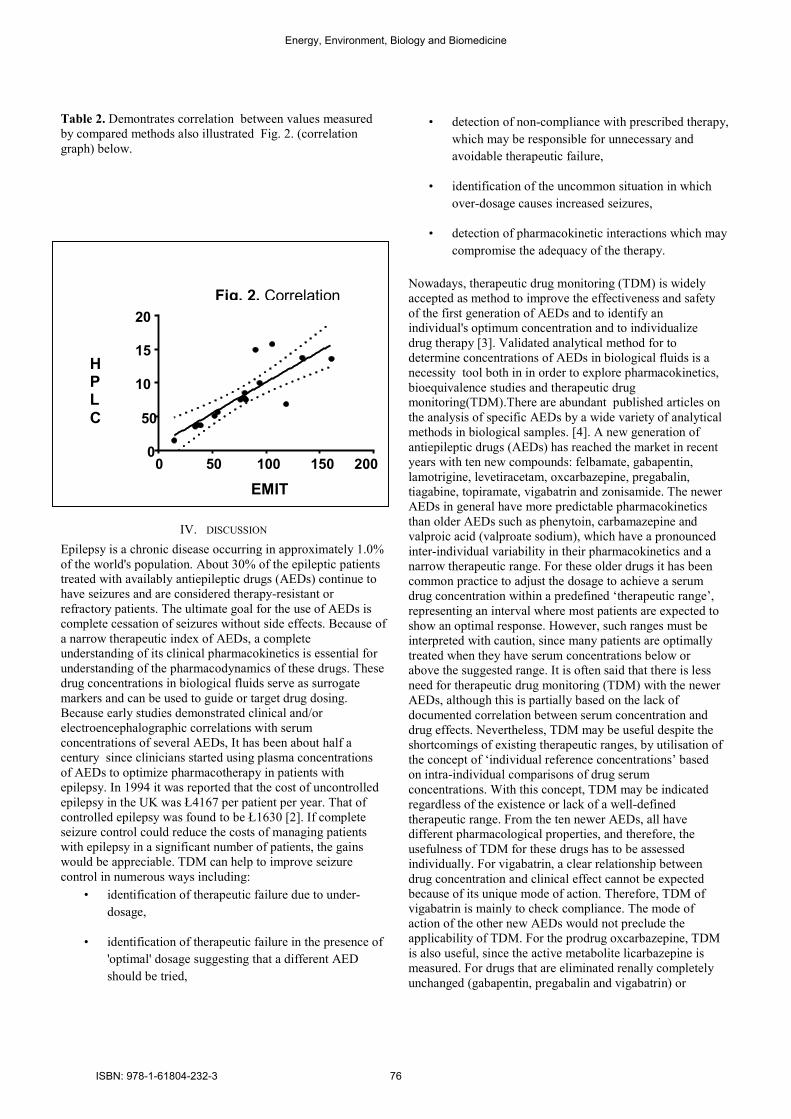
Table 2. Demontrates correlation between values measured

by compared methods also illustrated Fig. 2. (correlation

graph) below.

IV. DISCUSSION

Epilepsy is a chronic disease occurring in approximately 1.0%

of the world's population. About 30% of the epileptic patients

treated with availably antiepileptic drugs (AEDs) continue to

have seizures and are considered therapy-resistant or

refractory patients. The ultimate goal for the use of AEDs is

complete cessation of seizures without side effects. Because of

a narrow therapeutic index of AEDs, a complete

understanding of its clinical pharmacokinetics is essential for

understanding of the pharmacodynamics of these drugs. These

drug concentrations in biological fluids serve as surrogate

markers and can be used to guide or target drug dosing.

Because early studies demonstrated clinical and/or

electroencephalographic correlations with serum

concentrations of several AEDs, It has been about half a

century since clinicians started using plasma concentrations

of AEDs to optimize pharmacotherapy in patients with

epilepsy. In 1994 it was reported that the cost of uncontrolled

epilepsy in the UK was Ł4167 per patient per year. That of

controlled epilepsy was found to be Ł1630 [2]. If complete

seizure control could reduce the costs of managing patients

with epilepsy in a significant number of patients, the gains

would be appreciable. TDM can help to improve seizure

control in numerous ways including:

• identification of therapeutic failure due to under-

dosage,

• identification of therapeutic failure in the presence of

'optimal' dosage suggesting that a different AED

should be tried,

• detection of non-compliance with prescribed therapy,

which may be responsible for unnecessary and

avoidable therapeutic failure,

• identification of the uncommon situation in which

over-dosage causes increased seizures,

• detection of pharmacokinetic interactions which may

compromise the adequacy of the therapy.

Nowadays, therapeutic drug monitoring (TDM) is widely

accepted as method to improve the effectiveness and safety

of the first generation of AEDs and to identify an

individual's optimum concentration and to individualize

drug therapy [3]. Validated analytical method for to

determine concentrations of AEDs in biological fluids is a

necessity tool both in in order to explore pharmacokinetics,

bioequivalence studies and therapeutic drug

monitoring(TDM).There are abundant published articles on

the analysis of specific AEDs by a wide variety of analytical

methods in biological samples. [4]. A new generation of

antiepileptic drugs (AEDs) has reached the market in recent

years with ten new compounds: felbamate, gabapentin,

lamotrigine, levetiracetam, oxcarbazepine, pregabalin,

tiagabine, topiramate, vigabatrin and zonisamide. The newer

AEDs in general have more predictable pharmacokinetics

than older AEDs such as phenytoin, carbamazepine and

valproic acid (valproate sodium), which have a pronounced

inter-individual variability in their pharmacokinetics and a

narrow therapeutic range. For these older drugs it has been

common practice to adjust the dosage to achieve a serum

drug concentration within a predefined ‘therapeutic range’,

representing an interval where most patients are expected to

show an optimal response. However, such ranges must be

interpreted with caution, since many patients are optimally

treated when they have serum concentrations below or

above the suggested range. It is often said that there is less

need for therapeutic drug monitoring (TDM) with the newer

AEDs, although this is partially based on the lack of

documented correlation between serum concentration and

drug effects. Nevertheless, TDM may be useful despite the

shortcomings of existing therapeutic ranges, by utilisation of

the concept of ‘individual reference concentrations’ based

on intra-individual comparisons of drug serum

concentrations. With this concept, TDM may be indicated

regardless of the existence or lack of a well-defined

therapeutic range. From the ten newer AEDs, all have

different pharmacological properties, and therefore, the

usefulness of TDM for these drugs has to be assessed

individually. For vigabatrin, a clear relationship between

drug concentration and clinical effect cannot be expected

because of its unique mode of action. Therefore, TDM of

vigabatrin is mainly to check compliance. The mode of

action of the other new AEDs would not preclude the

applicability of TDM. For the prodrug oxcarbazepine, TDM

is also useful, since the active metabolite licarbazepine is

measured. For drugs that are eliminated renally completely

unchanged (gabapentin, pregabalin and vigabatrin) or

Fig. 2. Correlation

EMIT

0 50 100 150 200 0

50

100

150

200

HP L

C


ISBN: 978-1-61804-232-3 76

mainly unchanged (levetiracetam and topiramate), the

pharmacokinetic variability is less pronounced and more

predictable. However, the dose-dependent absorption of

gabapentin increases its pharmacokinetic variability. Drug

interactions can affect topiramate concentrations markedly,

and individual factors such as age, pregnancy and renal

function will contribute to the pharmacokinetic variability of

all renally eliminated AEDs. For those of the newer AEDs

that are metabolised (felbamate, lamotrigine, oxcarbazepine,

tiagabine and zonisamide), pharmacokinetic variability is

just as relevant as for many of the older AEDs. Therefore,

TDM is likely to be useful in many clinical settings for the

newer AEDs. The purpose of the present review is to discuss

individually the potential value of TDM of these newer

AEDs, with emphasis on pharmacokinetic variability. [5].

The rationale for the determination of AEDs and their

metabolites in body fluids and tissues arises from different

fields of investigations and clinical situations. Either drug or

metabolites levels are required for regular monitoring of

therapeutic drug levels, for adverse drug reactions, for drug-

drug interaction studies, for issues of toxicity concern, for

pharmacokinetic, pharmacokinetic/pharmacodynamic and

bioequivalence studies. AEDs are often used in

polypharmacy including up to three different AEDs, each of

them having several own metabolites [6]. TDM is more

important for drugs with a narrow therapeutic range, where a

correlation has been established between drug concentration

and its therapeutic and toxic effects. Although reasonably

well-defined target ranges in serum concentrations have

been determined for most of the established AEDs [7, 8]., it

should be remembered that these ranges only became

established after the development and general availability of

sensitive and reliable analytical methods. Thus, even though

phenobarbital and phenytoin became use for clinical

application in the early 1900s, after the development of

analytical methods in the 1960s, it was only since the early

1970s that target ranges were identified [9, 10].. Since then,

monitoring AEDs such as carbamazepine, vaproate and

ethosuximide has also become widely accepted in clinical

practice [11]. Although the target ranges have been defined

for some of the AEDs, the true therapeutic range is defined

for a given patient as the concentration that prevents

occurrence of epileptic episodes without causing side

effects. Since 1989, several AEDs have been have been

approved for clinical use, and because their regulatory trials

were not serum concentration controlled or designed to

investigate the relationship drug concentration and effect,

the value of monitoring these drugs is presently

controversial. However, some of the newer AEDs have

pharmacological properties suggesting that their optimal use

may be facilitated by use of TDM, and this has been the

subject of recent valuable debate [12, 13]. The AEDs have

been measured by a wide variety of analytical methods in

serum, blood, saliva, urine and tissue. For the classic AEDs

(carbamazepine, ethosuximide, phenobarbital, vaproate) and

some of the new AEDs (felbamate, topiramate, zonisamide

etc), automated enzyme-multiplied immunoassay technique

(EMIT) and fluorescence polarization immunoassays (FPIA)

are available and allow rapid and accurate determination of

concentrations in biological fluids, usually serum or plasma.

For other AEDs laboratories rely on chromatographic

methods; gas-chromatography (GC) and high-performance

liquid chromatography (HPLC) with a various detection

methods, which are more labor-intensive and relatively more

expensive. A number of simultaneous chromatographic

assays for AEDs have been developed in the past. The early

initial simultaneous AED assays, from 1970s and 1980s,

concentrated on separating the older AEDs such as

ethosuximide, primidone, carbamazepine, carbamazepine-

10,11-epoxide, phenytoin, and phenobarbital ([14-18] Many

subsequent assays separated the same compounds with the

inclusion or removal of one or more additional drugs or

metabolites such as ethylpenacemide [16], 5-

parahydroxyphenyl-5-phenylhydatoin, N-

desmethylmethsuximide [17]. and lamotrigine and phenyl-2-

theyl-malonamide [19]. Another inclusive assay separated

ethosuximide, primidone, carbamazepine, phenytoin,

Phenobarbital, carbamazepine metatabolites, phenobabital

metabolite and felbamate [20]. All of these assays employ

ultraviolet (UV) detection, thereby increasing the risk of

metabolite or metrix interferences. Assay developed over

past 15 years have focused more separating newer AEDs.

There are also new technological advance in the use of

capillary electrophoresis (CE) for TDM. Like other

chromatographic methods, CE allows simultaneous

measurement of several AEDs and can provide automation

of procedures, low cost, and rapid speed with high

specificity [21, 22]. The number of articles with the

analytical assay of AEDs in various biological matrices is

increasing in accordance with growing interest in the

situations with pharmacokinetic, TDM and bioequivalence

studies of clinical and research fields. The present review

was to focus to current technologies applied to the analysis

of AEDs in biological media for monitoring individual

AEDs or simultaneous monitoring of AEDs in recent years.

Levetiracetam is among the latest AEDs to be licensed for

clinical use indicated for adjunctive treatment of intractable

partial seizures that do not respond to other AEDs. Its

mechanism of action is not clearly defined, [23], wheras its

pharmacokinetics such as rapidly absorption from the

gastrointestinal tract, non-significant protein binding and

exhibition of linear pharmacokinetics.is well kown It is

minimally metabolised and excreted essentially unchanged

via the kidneys. Levetiracetam has no propensity to interact

with other AEDs [24].There is little published information

on levetiracetam blood levels in patients with epilepsy.

Nevertheless, audit of the clinical trials data for

levetiracetam suggests a target range of 35 - 110 µmol/L,

while blood levels can be measured by HPLC with

ultraviolet detection [25]. Levetiracetam is relatively a new

antiepileptic drug prescribed for the treatment of patients

with refractory partial seizures with or without secondary

generalization as well as for the treatment of juvenile

myoclonic epilepsy. A rapid and specific method by high-

performance liquid chromatography diode array detection

was developed to measure the concentration of levetiracetam

in human plasma. A wide variability in concentration-

response relationships was observed in patients.


ISBN: 978-1-61804-232-3 77

Nevertheless, the levetiracetam plasma concentration could

be used to help clinicians detect severe intoxication or to

verify compliance by repeating the measurement in patients

[26]. An isocratic high performance liquid chromatographic

micromethod, Ratnaraj et al. reported that no interference

from commonly prescribed antiepileptic drugs

(carbamazepine and its metabolite carbamazepine epoxide,

ethosuximide, gabapentin, lamotrigine, phenobarbitone,

phenytoin, primidone, valproic acid, and vigabatrin) was

observed, and thus the method can be used to monitor

levetiracetam in patients on polytherapy antiepileptic drug

regimens. [27]. In a study to evaluate the efficacy and

tolerability of levetiracetam (LEV) as add-on therapy in

children with refractory epilepsies and to determine the

value of LEV blood level monitoring in this population,

Giroux et al published that the most frequently observed

adverse effects were drowsiness, behavioral difficulties,

increase in seizure frequency and headaches. The majority

(60.5%) of the responders received doses between 10 and

50mg/kg/day and had a plasma concentration between 5 and

40microg/ml, however, no clear correlation between drug

plasma concentration and efficacy has been found. [28].

According to the study to evaluate the efficacy and

tolerability of Levetiracetam in a large pediatric cohort with

drug-resistant epilepsy from a prospective multicenter

observational study it has been reported that Levetiracetam

is a well-tolerated new antiepileptic drug that may

effectively improve seizure control as an add-on drug in

resistant epilepsy in childhood with good tolerability,

however, neurologically handicapped children appear at

increased risk for reversible neurocognitive side effects and

have a poorer treatment response. [29] Levetiracetam is

among the most recently licensed antiepileptic drug (AED)

for adjunctive therapy of partial seizures. Its mechanism of

action is uncertain but it exhibits a unique profile of

anticonvulsant activity in models of chronic epilepsy. [30].

Most studies suggest that levetiracetam is effective against

partial and generalized epilepsy. In resistant partial epilepsy,

the percentage of responders reaches 64%, with 8 to 23%

seizure free. Levetiracetam is used to treat symptomatic and

idiopathic epilepsies. The drug has also proven effective

against photosensitivity and epileptic and nonepileptic

myoclonus. The most frequent side effects involve the

behavioral sphere and manifest mostly in patients with a

history of behavioral problems. In some patients,

levetiracetam increases the number of seizures, but this

adverse reaction can be partially avoided with slow titration.

Doses for children should be 130 to 140% of those advised

for adults. [31]. Treatment of seizures in pediatric patients is

complicated by the fact that the etiology of the disorder and

the pharmacokinetics, efficacy, and safety of antiepileptic

drugs may differ from that in adults. With few controlled

clinical trials of AEDs in children, the selection of agents to

treat paediatric patients must be made on the basis of

information from small uncontrolled studies or the

extrapolation of clinical trial results in adults. Data from a

large number of children with a wide range of seizure

disorders who were treated in small-scale prospective

studies, or whose records were retrospectively evaluated,

indicate that levetiracetam reduces the frequency of seizures

in pediatric patients. Available data also indicate that

levetiracetam is well tolerated in pediatric patients, with a

safety profile similar to that in adults, a low potential for

behavioral disturbances, and no reported idiosyncratic

adverse reactions. As with other AEDs, children metabolize

and clear levetiracetam more rapidly than adults, and

somewhat higher doses (based on body weight) are needed

to achieve desired plasma concentrations. Several ongoing

studies will provide further information on the

pharmacokinetics, efficacy, and safety of levetiracetam in

this patient population.[32]. Some study results support the

use of a weight-based LEV dosing regimen and provide a

basis for a recommended pediatric dosage regimen, but the

relationship between LEV plasma concentrations and

clinical effect has not been evaluated fully and could differ

between adults and children and Clinical studies should be

able to validate these dosing recommendations. [33]. Some

significant covariates for pharmacokinetics of levetiracetam

were identified: (a) age on the absorption rate constant ; (b)

bodyweight, dose, clearance, and concomitant enzyme-

inducing AED on plasma oral clearance (CL/F); and (c)

bodyweight on the apparent volume of distribution after oral

administration (V(d)/F). The main explanatory covariates

were age on absorption rate constant, bodyweight on CL/F

and V(d)/F, and enzyme-inducing AED on CL/F, of which

bodyweight was the most influential covariate. However, the

most influential covariate of levetiracetam pharmacokinetics

in children is bodyweight. [34]. Both serum and CSF

levetiracetam concentrations rose essentially linearly and

dose-dependently, suggesting that transport across the

blood-brain barrier is not rate limiting over the levetiracetam

concentration range observed. However, while apparent

elimination half-life (t1/2) values for both serum and CSF

were dose-independent (mean value range 1.8-2.8 and 4.4-

4.9 h, respectively), t1/2 values for CSF were significantly

larger. As the serum free/total serum levetiracetam

concentration ratio (free fraction) was 1.01+/-0.02 (mean+/-

S.E.M.), it can be concluded that levetiracetam is not protein

bound. [35]. Levetiracetam is completely and rapidly

(Tmax, 1 h) absorbed after oral ingestion with

bioavailability of 100% [36, 37]. Although drug-food

interactions do not show on the extent of absorption, rate of

absorption is slowed in the presence of food. Administration

of a crushed LVT tablet together with 120 ml of an entral

nutrition formula has been associated with a mean 27%

decrease in peak LVT concentration, but the effect was not

statistically significant. [38]. Levetiracetam shows linear

pharmacokinetic and renal elimination with approximately

66% of a dose eliminated unchanged and 27% as inactive

metabolite [39]. The relationship between LVT serum

concentrations and clinical effect has not been ascertained,

and consequently the value of serum concentrations

measurements is not established. Because of its favorable

therapeutic index, low plasma protein binding and minimal

side-effect profile, routine monitoring of LVT serum

concentrations appears to be unnecessary for safe use of the

drug, and dosing can be readily guided by the therapeutic

response [40, 41]. Nevertheless, its use in ascertaining


ISBN: 978-1-61804-232-3 78

compliance and managing patients that are overdosed

would be helpful. Because LVT has a relatively short half-life,

sampling time in relation to dose ingestion is important for the

interpretation of the drug concentration. Ideally samples for

LVT measurements should be drawn before the morning dose.

Because LVT can undergo in vitro hydrolysis, it is important

to separate whole blood from serum as soon as possible so as

to avoid LVT hydrolysis that would result in spuriously lower

concentrations being measured [42]. Although AED

monitoring in saliva may some clinical applicability, it has not

yet come into routine use, but, a significant positive

correlation exists between LVT saliva and serum

concentrations, LVT like other AEDs, can be measures in

saliva as an alternative to blood-based assays for minotoring

the LVT therapy [43, 44]. Numerous chromatographic

methods have been reported for the quantification of LVT in

biological fluids. Different HPLC methods for the

determination of LVT in human plasma have been reported

coupled with UV [45, 46]. or diode array detection [47, 48].

mostly after sample pretreatment by expensive solid-phase

extraction or time-consuming liquid-liquid extraction

procedures [46, [48]. The availability of simple, accurate and

inexpensive analytical assays is crucial for the successful use

of TDM in clinical practice. LVT spiked plasma sample

preparation by different kinds of deproteinization before

HPLC-diode array detection was first explored by Pucci et

al[47], and subsequently applied to patient samples analysis by

HPLC-UV [49, 45, 50]. Otherwise, these involve GC-NPD

[51]. and GC-MS [52]. Most of the reported methods lack

selectivity, sensitivity, and reliability. They encounter also

problems particularly tedious and time-consuming sample

preparation as well as high sample volume. Recently, LC-

tandem MS is considered a gold standard to utilize in analysis

of drugs in biological fluids. The high sample throughput,

selectivity and sensitivity for analytes of interest may increase

the applicability of tandem MS in clinical chemistry as well as

clinical studies [53-55].

V. CONCLUSIONS

We found that there is excellent correlation as already

published by some authors used other methods including

HPLC and UPLC with tandem weight spectrometry.

Potencially toxic level is considered as any levels > 37 umol/l,

but great concern should be given for existing inter and intra

individual variability.Our method is suitable for routins

levetriracetam plasma level determination in the process of

therapeutic drug monitoring.

References

[1]. Cormier J, Chu CJ. Safety and efficacy of levetiracetam

for the treatment of partial onset seizures in children from one

month of age. Neuropsychiatr Dis Treat. 2013;9:295-306

[2]. Cockerell OC, Hart YM, Sander JWAS, et al. The cost of

epilepsy in the United Kingdom: an estimation based on two

population-based studies. Epilepsy Res 1994; 18: 249-260

[3]. Anderson GD. Pharmacokinetic, Pharmacodynamic, and

pharmacogenetic targeted therapy of antiepileptic drugs.

Ther Drug Monit 2008;30:173–180.)

[4]. Juseop Kang, Yoo-Sin Park, Shin-Hee Kim, Sang-Hyun

Kim, and Min-Young Jun. Modern Methods for

Analysis of Antiepileptic Drugs in the Biological

Fluids for Pharmacokinetics, Bioequivalence and

Therapeutic Drug Monitoring. Korean J Physiol

Pharmacol. 2011 Apr;15(2):67-81)

[5]. Svein I. Johannessen, Torbjörn Tomson.

Pharmacokinetic Variability of Newer Antiepileptic Drugs

.Clinical Pharmacokinetics November 2006, Volume 45,

Issue 11, pp 1061-1075)

[6]. Chollet DF. Determination of antiepileptic drugs in

biological material. J Chromatogr B Analyt Technol Biomed

Life Sci 2002;767:191–233

[7]. Johannessen SI. Plasma drug concentration monitoring

of anticonvulsants: practical guidelines. CNS Drugs

1997;7:349–365)

[8]. Eadie MJ. Therapeutic drug monitoring-antiepileptic

drugs. Br J Clin Pharmacol 1998;46:185–193

[9]. Buchthal F, Svensmark O. Aspects of pharmacology of

phenytoin (dilantin) and phenobarbital relevant to their

dosage in the treatment of epilepsy. Epilepsia 1960;1:373–

384.

[10]. Kutt H, Penry JK. Usefulness of blood levels of

antiepileptic drugs. Arch Neurol 1974;31:283–288

[11]. Johannessen SI, Battino D, Berry DJ, Bialer M,

Kramer G, Tomson T, Patsalos PN. Therapeutic drug

monitoring of the newer antiepileptic drugs. Ther Drug

Monit 2003;25:347–363

[12]. Patsalos PN. New antiepileptic drugs. Ann Clin

Biochem 1999;36:10–19.)

[13]. Glauser TA, Pippenger CE. Controversies in blood-

level monitoring; reexamining its role in the treatment of

epilepsy. Epilepsia 2000;41 Suppl 8:S6–S15

[14]. Soldin SJ, Hill JG. Rapid micromethod for measuring

anticonvulsant drugs in serum by high-performance liquid

chromatography. Clin Chem 1976;22:856–859.


ISBN: 978-1-61804-232-3 79

[15]. Kabra PM, Stafford BE, Marton LJ. Simultaneous

measurement of phenobarbital, phenytoin, primidone,

ethosuximide, and carbamazepine in serum by high-

performance liquid chromatography. Clin Chem

1977;23:1284–1288.

[16]. Christofides JA, Fry DE. Measurement of

anticonvulsants in serum by reversed-phase ion-pair liquid

chromatography. Clin Chem 1980;26:499–50

[17]. Ou CN, Robnerud CL. Simultaneous measurement of

ethosuximide, primidone, phenobarbital, phenytoin,

carbamazepine, and their bioactive metabolites by liquid

chromatography. Clin Chem 1984;30:1667–1670

[18]. Juergens U. Simultaneous determination of zonisamide

and none other antiepileptic drugs and metabolites in serum.

A comparison of microbore and conventional high-

performance liquid chromatography. J Chromatogr

1987;385:233–240

[19]..Lanças FM, Sozza MA, Queiroz ME. Simultaneous

plasma lamotrigine analysis with carbamazepine,

carbamazepine-10,11-epoxide, primidone, phenytoin,

phenobarbital, and PEMA by micellar electrokinetic

capillary chromatography (MECC). J Anal Toxicol

2003;27:304–308.

[20]. Romanyshyn LA, Wichmann JK, Kucharczyk N,

Shumaker RC, Ward D, Sofia RD. Simultaneous

determination of felbamate, primidone, Phenobarbital,

carbamazepine, two carbamazepine metabolites, phenytoin

and one phenytoin metabolite in human plasma by high-

performance liquid chromatography. Ther Drug Monit

1994;16:90–99

[21]. Kataoka Y, Makino K, Oishi R. Capillary

electrophoresis for therapeutic drug monitoring of

antiepileptics. Electrophoresis 1998;19:2856–2860.

[22]. Burton ME, Shaw LM, Schentag JJ. Antiepileptic

drugs. In: Garnett WR, Anderson GD, Collins RJApplied

pharmacokinetics & pharmacodynamics - principles of

therapeutic drug monitoring. 4th ed. Philadelphia: Lippincott

Williams & Wilkins; 2006. pp. 491).

[23]. Noyer M, Gillard M, Matagne A, Henichart JP,

Wulfert E. The novel antiepileptic drug levetiracetam (ucb

L059) appears to act via a specific binding site in CNS

membranes. Eur J Pharmacol 1995; 286, 137-146).

[24]. Patsalos PN Properties of antiepileptic drugs in the

treatment of idiopathic generalized epilepsies. Epilepsia

2005;46 Suppl 9:140-8.

[25]. Ratnaraj N, Doheny HC, Patsalos PN. A micromethod

for the determination of the new antiepileptic drug

levetiracetam (ucb-LO59) in serum or plasma by high

performance liquid chromatography. Ther Drug Monit 1996;

18: 154-157

[26]. Lancelin F, Franchon E, Kraoul L, et al. Therapeutic

Drug Monitoring of Levetiracetam by High-Performance

Liquid Chromatography With Photodiode Array Ultraviolet

Detection: Preliminary Observations on Correlation

Between Plasma Concentration and Clinical Response in

Patients With Refractory Epilepsy. Ther Drug Monit

2007;29:576-583

[27]. Ratnaraj N, Doheny HC, Patsalos PN. A micromethod

for the determination of the new antiepileptic drug

levetiracetam (ucb LO59) in serum or plasma by high

performance liquid chromatography. Ther Drug Monit.

1996;18:154-7

[28]. Giroux PC, Salas-Prato M, Théorêt Y, Carmant L.

Levetiracetam in children with refractory epilepsy: lack of

correlation between plasma concentration and efficacy.

Seizure. 2009;18:559-63

[29]. Opp J, Tuxhorn I, May T, Kluger G, Wiemer-Kruel A,

Kurlemann G, Gross-Selbeck G, Rating D, Brandl U,

Bettendorf U, Härtel C, Korn-Merker Levetiracetam in

children with refractory epilepsy: a multicenter open label

study in Germany. Seizure. 2005;14:476-84

[30]. 29. Pinto A, Sander JW.Levetiracetam: a new

therapeutic option for refractory epilepsy. Int J Clin Pract.

2003;57:616-21

[31]. Vigevano F. Levetiracetam in pediatrics. J Child

Neurol. 2005;20:87-93

[32]. Glauser TA, Dulac O. Preliminary efficacy of

levetiracetam in children. Epileptic Disord. 2003;5 Suppl

1:S45-50

[33]. Chhun S, Jullien V, Rey E, Dulac O, Chiron C, Pons

G. Population pharmacokinetics of levetiracetam and dosing

recommendation in children with epilepsy. Epilepsia. 2009

;50:1150-7

[34] Toublanc N, Sargentini-Maier ML, Lacroix B, Jacqmin

P, Stockis A. Retrospective population pharmacokinetic

analysis of levetiracetam in children and adolescents with

epilepsy: dosing recommendations. Clin Pharmacokinet.

2008;47:333-41

[35]. Doheny HC, Ratnaraj N, Whittington MA, Jefferys JG,

Patsalos PN. Blood and cerebrospinal fluid

pharmacokinetics of the novel anticonvulsant levetiracetam

(ucb L059) in the rat. Epilepsy Res. 1999;34:161-8.

[36]. Nash EM, Sangha KS. Levetiracetam. Am J Health

Syst Pharm 2001;58:1195–1199.

[37]. Ramael S, De Smedt F, Toublanc N, Otoul C,

Boulanger P, Riethuisen JM, Stockis A. A Single-dose

bioavailability of levetiracetam intravenous infusion relative

to oral tablets and multiple-dose pharmacokinetics and

tolerability of levetiracetam intravenous infusion compared

with placebo in healthy subjects. Clin Ther 2006;28:734–

744

[38]. Fay MA, Sheth RD, Gidal BE. Oral absorption kinetics

of levetiracetam: the effect of mixing with food or enteral

nutrition formulas. Clin Ther 2005;27:594–598.

[39]. Patsalos PN. Clinical pharmacokinetics of

levetiracetam. Clin Pharmacokinet 2004; 43:707–724

[40]. Johannessen SI, Battino D, Berry DJ, Bialer M,

Kramer G, Tomson T, Patsalos PN. Therapeutic drug

monitoring of the newer antiepileptic drugs. Ther Drug

Monit 2003;25:347–363

[41] . Tomson T, Johannessen SI. Therapeutic monitoring of

the new antiepileptic drugs. Eur J Clin Pharmacol

2000;55:697-705

[42]. Patsalos PN, Ghattaura S, Ratnaraj N, Sander JW. In situ

metabolism of levetiracetam in blood of patients with

epilepsy. Epilepsia 2006;47:1818–1821.


ISBN: 978-1-61804-232-3 80

[43]. Grim SA, Ryan M, Miles MV, Tang PH, Strawsburg

RH, deGrauw TJ, Fakhoury TA, Baumann RJ. Correlation of

levetiracetam concentrations between serum and saliva. Ther

Drug Monit 2003;25:61–66.

[44]. Mecarelli O, Li Voti P, Pro S, Romolo FS, Rotolo M,

Rulitano P, Accornero N, Vanacore N. Saliva and serum

levetiracetam concentrations in patients with epilepsy. Ther

Drug Monit 2007;29:313–318

[45]. Martens-Lobenhoffer J, Bode-Böger SM. Determination

of levetiracetam in human plasma with minimal sample

pretreatment. J Chromatogr B Analyt Technol Biomed Life

Sci 2005;819:197–200

[46]. Juenke J, Brown PI, Urry FM, McMillin GA. Drug

monitoring and toxicology: a procedure for the monitoring of

levetiracetam and zonisamide by HPLC-UV. J Anal Toxicol

2006;30:27–30

[47]. Pucci V, Bugamelli F, Mandrioli R, Ferrranti A,

Kenndler E, Raggi MA. High-performance liquid

chromatographic determination of Levetiracetam in human

plasma: comparison of different sample clean-up procedures.

Biomed Chromatogr 2004;18:37–44

[48]. Lancelin F, Franchon E, Kraoul L, Garciau I, Brovedani

S, Tabaouti K, Landr÷ E, Chassoux F, Paubel P, Piketty ML.

Therapeutic drug monitoring of levetiracetam by high-

performance liquid chromatography with photodiode array

ultraviolet detection: preliminary observations on correlation

between plasma concentration and clinical response in patients

with refractory epilepsy. Ther Drug Monit 2007;29:576-583.

[49]. Ramael S, De Smedt F, Toublanc N, Otoul C, Boulanger

P, Riethuisen JM, Stockis A. A Single-dose bioavailability of

levetiracetam intravenous infusion relative to oral tablets and

multiple-dose pharmacokinetics and tolerability of

levetiracetam intravenous infusion compared with placebo in

healthy subjects. Clin Ther 2006;28:734–744

[50]. Contin M, Mohamed S, Albani F, Riva R, Brauzzi A.

Simple and validated HPLC-UV analysis of levetiracetam in

deproteinized plasma of patients with epilepsy. J Chromatogr

B Analyt Technol Biomed Life Sci 2008;873:129–132

[51].Vermeij TA, Edelbroek PM. High-performance liquid

chromatographic and megabore gas-liquid chromatographic

determination of levetiracetam (ucb L059) in human serum

after solid-phase extraction. J Chromatogr B Biomed Appl

1994;662:134–139

[52]. Isoherranen N, Roeder M, Soback S, Yagen B, Schurig

V, Bialer M. Enantioselective analysis of levetiracetam and its

enantiomer R-alpha-ethyl-2-oxo-pyrrolidine acetamide using

gas chromatography and ion trap mass spectrometric

detection. J Chromatogr B Biomed Sci Appl 2000;745:325–

332

[53. Jain DS, Subbaiah G, Sanyal M, Pal U, Shrivastav PS.

Determination of levetiracetam in human plasma by liquid

chromatography/electrospray tandem mass spectrometry and

its application to bioequivalence studies. Rapid Commun

Mass Spectrom 2006;20:2539–2547 [54]. Guo T, Oswald LM,

Mendu D, Soldin SJ. Determination of levetiracetam in human

plasma/serum/saliva by liquid chromatography-electrospray

tandem mass spectrometry. Clin Chim Acta 2007;375:115–

118

[55]. Matar KM. Quantification of levetiracetam in human

plasma by liquid chromatography-tandem mass spectrometry:

application to therapeutic drug monitoring. J Pharm Biomed

Anal 2008;48:822–828.


ISBN: 978-1-61804-232-3 81

Abstract—Bibliographic data and the results of present domestic

experiments show that Paulownia species can be grown easily, have high biomass production, favourable energetic parameters and modest requirements as to site quality. Establishment of Paulownia plantations may support the aim to meet the growing needs for site-remediation and biomass for energy purposes. This paper gives an overlook on the relevant research activity and results of the University of West Hungary. The use of the selected species can reasonably be recommended for these purposes, since the plantations - grown from self-developed propagating material, managed and tested according to the formulated methods - have a high production of biomass and thus confirmed as suitable for energy purposes. The use of Paulownia for agroforestry pruposes may also be a prospective way of multifunctional landuse while providing beneficial ecosystem services.

Keywords— energy, biomass, Paulownia, agroforestry.

I. INTRODUCTION HE empress tree (Paulownia tomentosa) is one of the world’s most multifaceted tree species. It originates from China and are also grown throughout Asia, USA, Australia

and Europe. (AFBI, 2008) Its wide spectrum of utilization ranges from industrial use (furniture, timber, pulp and paper, energy), to medical and hive products, or decoration (eg. onamental trees and wood carvings). In recent years the awareness and business interest for Paulownia is growing fast in Central-Eastern Europe, while there is a lack of research activities in the subject of cultivation , utilization, and adoption of the best practices in these countries. However it is of utmost importance to take the local conditions into consideration when adopting new species and technologies. As no preliminary research activity can be recognized on this subject in Hungary, NyME KKK together with external partners (cooperative and farmers) started a research program on energy and agroforestry use of Paulownia.

A. Vityi is with the University of West Hungary Institute of Forestry and Environmental Techniques, and with the UWH Cooperational Research Centre Nonprofit Ltd., Bajcsy-Zs. u. 4. Sopron, H-9400, Hungary (e-mail: [email protected])

B. Marosvölgyi is with the University of West Hungary Cooperational Research Centre Nonprofit Ltd., Bajcsy-Zs. u. 4. Sopron, H-9400, Hungary (e-mail: [email protected])

II. MATERIAL AND METHOD According to the literature, Paulownia can be multiplied from seeds, cuttings or by micropropagation. (Al-Tinawi, I. A. et al., 2010, Lobona, S., 2008) (Gyuleva, V., 2008) In favourable conditions a 10 year-old tree may reach 30-40 cm in diameter, 10-12 m in height and provide 0,2-0,6 m3 volume production. (Yang, 2004)

In the first stage of our experiments we used selected mother plants and developed a special method of propagation form seeds. The method is based on a special substrate composition and strict planting protocol. In spring seedlings with 4-6 leaves were relocated into planting containers where they grew until planting out in autumn.(Image 1)

Image 1 Selected Paulownia seedlings in spring 2006. (Picture made by the Authors)

The first experimental bioenergy plantations were established from this selected material in autumn 2006. Planting and research activities were coordinatd by the Eco-energetic Research Division of NyME KKK. Plantations were located in various parts of the country with different climate conditions. Also different planting structures and cutting rotation systems were applied in order to examine the growing and other relevant parameters of the plants. In order to scan the usability of the trees in energetic processes we studied the international literature available on Paulownia, then made tests with the samples originated from our own plantations on bulk density, moisture content, ash content, and heating value, which are basic parameters concerning energetic utilization.

New tree species for agroforestry and energy purposes

Andrea Vityi, Béla Marosvölgyi

T


ISBN: 978-1-61804-232-3 82



III. RESULTS AND CONCLUSIONS

A. Experiences on propagation, planting and plant management

By the use of specifically selected Paulownia plants and self-developed propagation method we managed to realize 80% plant survival. Further experimental plantations based on the selected material are planned to be established for extended research purposes in the next years.

B. Experimental results of biomass production According to the results of the crop yield survey the

biomass production of the experimental plantation was definitely high (55 t/ha).

Image 2 The 6-year-old experimental plantation with one-/two-year cutting rotation (2012 October). Seedlings were planted in double-rows taking the needs of harvesting technology into

account. (Source: Vityi-Marosvölgyi,2012)

It has to be underlined that the given high yield volume is

only valid under the specific parameters of the experimental system (applied planting structure, site conditions, selected material, cutting rotation, site management, etc.). Furthermore, given the dimensions of the test parcel, we had to calculate with border-effect which surely had significant benefits for the biomass production volume.

Image 3 Cross-sectional view of a 4-year tree form a Hungarian bioenergy test plantation with selected

Paulownia tomentosa (replanting system) (Source: Vityi-Marosvölgyi,2011)

Image 4 Energy-wood from a Hungarian Paulownia tomentosa experimental site (from one stem)

(Source: Vityi-Marosvölgyi, 2011)

C. Results of the energetic analyses of the biomass form the Paulownia experimental site

Having studied the literature we found that the available data on certain energetic parameters of Paulownia-biomass varied, but basically were comparable with the results of our measurements.(Table 1) (Source: Vityi-Marosvölgyi,2012)

The good test results of the woody biomass from the

experimental sites - whether in annual cutting rotation or in multi-year rotation system - show that Paulownia may definitely be suitable for energy purposes.


ISBN: 978-1-61804-232-3 83

Mechanical and

combustion parameters of the one-year-old shoot of selected

Paulownia tomentosa variety

Bibliographical data on the mechanical and

combustion parameters of

Paulownia species

wood

bark mean*

Bulk density (g/cm3,, air-dry)

0,35 0,22-0,30

Moisture content (m/m%, air-dry)

11,80 10,90 11,61 7,74-10,00

Ash content (m/m%)

0,92 3,05 1,37 0,5-5,28

Heating value (MJ/kg, air-dry)

16,66 17,40 16,82

16,58-18,83

Heating value (MJ/kg, absolute dry)

18,92 19,67 19,10

*based on bark-rate of 21% measured from one-year-old shoot samples Table 1 Results of the University of West Hungary Cooperational Research Centre’s tests compared with the data available in the literature on the energetic parameters of Paulownia

D. The Use of Paulownia in agroforestry systems

Agroforestry is the practice of deliberately combining woody vegetation (trees and/or shrubs) with crop and/or livestock systems. Agroforestry practices help farmers to diversify farm income, while benefiting from the resulting ecological and economical interactions eg. improve soil and water quality, reduce erosion, pollution, or damage due to extreme weather, enhance resource efficiency, biodiversity, and the resiliency of the production system. Agroforestry systems manifest in several practices: forest buffers, windbreaks, silvopasture, alley cropping, forest farming, etc.

Based on the positive bibliographic data on the use of Paulownia in alley-cropping and the favorable results of NyME KKK’s field tests we decided to extend the examinations to the use of Paulownia for agroforestry purposes. Agroforestry experiments with Paulownia started in 2012. The initial step was the plantation of the first and so far only experimental Paulownia intercropping system in Hungary. In the next years NyME KKK plan to make investigations on crucial parameters of sustainable management of the Paulownia-intercrop systems. This activity will also be a contribution to EU FP7 project called „AGFORWARD”. This is a four-year pan-european project, with the goal of promoting appropriate agroforestry practices that advance sustainable rural development.

REFERENCES [1]. Al-Tinawi, I. A. et al.(2010): Development of In vitro

Propagation System for Paulownia tomentosa L. Using Tissue Culture Techniques. Jordan Journal of Agricultural Sciences, 6 (4), 2010

[2]. Gyuleva, V. (2008): Project “Establishment of geographical plantations of Paulownia elongata hybrids in Bulgaria” – contract No 37 with State Agency of Forests (2007–2010). Bulgarian Avademy of Sciences - News. No 12 (64), Year VI, 2008.

[3]. Lobna, S. Taha (2008): A Micropropagation Protocol of Paulownia kowakamii through in vitro culture technique. Australian Journal of Basic and Applied Sciences, 2(3): 594-600

[4]. Muthuri, C. W. et al. (2005): Tree and crop productivity in Grevillea, Alnus and Paulownia-based agroforestry systems in semi-arid Kenya. Forest Ecology and Management, 212: 23-39.

[5]. Vityi, A. – Marosvölgyi, B. (2011.): Hazai eredetű császárfa mint energianövény. Környezeti Kutatások. Környezeti Erőforrás-gazdálkodási és védelmi Kooperációs Kutatási Központ Nonprofit Kft., Ökoenergetikai Kutatási Főirány, Sopron.

[6]. Vityi, A. – Marosvölgyi, B. (2012.): A fajszi kísérleti Paulownia ültetvények újabb kutatási eredményei. Környezeti Erőforrás-gazdálkodási és védelmi Kooperációs Kutatási Központ Nonprofit Kft., Ökoenergetikai Kutatási Főirány, Sopron.

[7]. Woods, V.B. (2008): Paulownia as a novel biomass crop for Northern Ireland? A review of current knowledge. Occasional publication No. 7. Agri-Food and Biosciences Institute, Hillsborough, 2008.

[8]. Yang, X. (2004): Paulownia Agroforestry Systems in China. Poster. Preoceedings of the International Ecoagriculture Conference and Practitioners’ Fair. vol. 2: 21-22. Conference abstracts. Nairobi, 2004.


ISBN: 978-1-61804-232-3 84

Abstract— Background: Methotrexate (MTX) is one of the most widely used anti-cancer agents, and administration of high-dose methotrexate followed by leucovorin (LV) rescue therapy is an important component in the treatment of a variety of cancers. High-dose MTX is thought to be safe for administration in patients with normal renal function with concomitant alkalinization, hydration, and pharmacokinetically-guided leucovorin rescue. However, acute renal failure and other adverse outcomes are unavoidable under certain circumstances. High-dose methotrexate (HDMTX)-induced renal dysfunction can be a life threatening event, because it delays methotrexate excretion, thereby exacerbating the other toxicities of MTX. High-dose methotrexate -induced renal dysfunction continues to occur in patients with osteosarcoma who are treated on clinical protocols despite optimal supportive care. Approximately, 1.8% of patients with osteosarcoma, who received HDMTX may develope nephrotoxicity of various grade carring considerable mortality rate . High-dose methotrexate-induced renal dysfunction can be life threatening, because it delays methotrexate excretion, thereby exacerbating the other toxicities of methotrexate. HDMTX-induced nephrotoxicity

has been usually managed with high-dose leucovorin, dialysis-based methods of MTX removal, thymidine, and recently by adminstration of the recombinant enzyme, carboxypeptidase-G2 (CPDG2), which cleaves MTX to inactive metabolites. Objective: The aim of this paper is to describe the case of an adult Caucasian male patient with osteosercoma who presented with extremely delayed MTX clearance after high-dose administration conducted according to the EURAMOS protocol. In the presnt case, We discuss also the fate of the patient where delayed MTX excretion was a big challenge and finally managed using supportive measures including high doses of leucovorin and very effectively CPDG2 without having to adopt other invasive procedures like dialysis.

Keywords—Osteosarcoma,High-doseMXT, Nephro-Toxicity

I. INTRODUCTION

steosarcoma (osteogenic sarcoma) is the most common type of primary bone cancer most

occuring in children and young adults with peak incidences in adolescence and at age >60 years, but can occur at any age.[1] Methotrexate (MTX), a

Extremely delayed elimination of methotrexate in a young man with osteosarcoma:

A case study demonstrating an association with impaired renal function.

1Tesfaye H,1Beyerova M,1Jedlickova B, 2Korandova A,2Linke Z, 2Becvarova M, 3Shimota M.

1Department of Medical Chemistry and Clinical Biochemistry, Division of Clinical Pharmacology, 2Department of Oncology, Faculty Hospital in Motol, 2nd Faculty of Medicine, Charles University, Prague, Czech Republic., 3International Student (Faculty Member), 2nd Faculty of Medicine, Charles University, Prague, Czech Republic.

O


ISBN: 978-1-61804-232-3 85

classic antifolate is one of the most widely used and well studied anticancer agents, where the administration of MTX doses ≥ 1000 mg/m2 combined with leucovorin (LV) rescue is defined as high-dose methotrexate (HDMTX)and is an important component of treatment for a variety of malignancies, including osteosarcoma.[2] Todate, a very high-dose methotrexate usually >1 g/m2) administered as an intravenous infusion remains an important component in the treatment of variety of cancers inparticular for osteosarcoma, but this HDMTX treatment schedule carries a risk of nephrotoxicity among others. .[3] Data from a number of studies performed in the 1970s showed that a sustained elevation of serum MTX concentrations at 24 h (≥5 μmol/L), 48 h (≥1 μmo/L) and 72 h (≥0.1 μmo/L) after the start of the MTX infusion is considered to be toxic referring to the usual serum MTX level <0.1 μmol/L 48 h after HDMTX administration. In the era of optimal supportive care the incidence of grade 3–4 ARF after HDMTX has reportedly decreased markedly in solid-cancer patients. .[4] Although HDMTX-associated severe acute renal failure (ARF) is an infrequent, the very high doses of MTX generally used in solid-cancer patients such as with osteosarcoma , who receive a MTX dose >8 g/m2, the risk of severe ARF may be certainly higher. According to large case series, the reason why an individual patient comes prone to develop ARF after HDMTX despite modern supported care remains unexplained in the majority of cases (1-3) .[3],.[4], [5], but drug drug interactions are mostly unrecognized or overlooked.[6] In case of our patient the role of pre treatment with Cis-platin in the near past before the intial therapy with MXT may be the partial explation for the precipitation of acute renal dysfanction grade 2-3 (Renal toxicity

was graded using World Health Organization criteria (Grade 1, serum creatinine levels < 1.5 × ULN; Grade 2, 1.5–3.0 × ULN; Grade 3, 3.1–6.0 × ULN; and Grade 4, > 6.0 × ULN) Although the incidence and mortality of HDMTX-induced renal dysfunction appear to have decreased significantly since the 1970s, [7] nephrotoxicity continues to occur and may be fatal. Therefore, in situations,where usual care fails in patients with delayed MTX excretion and high plasma MTX concentrations, othermeasures like treatment by CPDG2 should be considered to lower plasma MTX concentrations rapidly and efficiently as previously recommended. [3] The median time to recovery of renal function for a numer of patients, as defined by the individual studies, was 16 days (range, 4–48 days)., where treatment of patients did not include carboxypeptidase-G2. According to published literature reviewed from 1977 to 2002 on recovery of renal function in patients with methotrexate-induced renal dysfunction, the median time to recovery of renal function for a numer of patients, as defined by the individual studies, was 16 days (range, 4–48 days)., where treatment of patients did not include carboxypeptidase-G2. [3], [8]

II. CASE DESCRIPTION

A 37-year-old Caucasian male had been treated initially had been treated initially with a combination of doxorubicin and cisplatin for proven diagnosis of osteosarcoma. Just after a month later, the patient was scheduled for methotrexate treatment according to the EURAMOS (European and American Osteosarcoma Study Group) protocol, a joint protocol of four of the world’s leading multi-institutional osteosarcoma groups; which uses a dose of 12 g/m2 over a 4-hour infusion and repeated with 11.34 g/m2. The concentration of MXT determined by fluorescent polarization immunoassay (FPIA) method 6 hours post-infusion showed levels within expected range. However,


ISBN: 978-1-61804-232-3 86

measurements taken 24 hours post-dose and later were extremely high. This indicated poor elimination and was also confirmed by significantly elevated serum creatinine (Fig. 1) as well as blood urea nitrogen. Drug plasma level monitoring was continued on a daily basis as per protocol guidelines until the level reached less than 0.1uM. This took one month +8 days from initial MXT administration.

0

200

400

600

800

1000

1200

1 3 5 7 9 11 13 15 17 19 21 23 25 27 29 31 33 35

Sampling interval (days) for the variables post methotrexate infusion

Con

cent

ratio

ns (U

mol

/L)

MXTS-CrBUN

Fig. 1. Extremely delayed methotrexate (MXT) elimination corresponding with serum creatinine levels (S-Cr) and persistence of high blood urea nitrogen (BUN) demonstrating significant renal function impairment. Taking into consideration that with high-dose methotrexate, toxic concentrations are generally considered to be: ≥ 5 µmol/L at 24 hours after the dose, ≥ 0.5 µmol/L at 48 hours, and ≥ 0.055 µmol/L at 72 hours; we declare our findings as potentially extremely toxic levels. The test results are used to guide the amount and timing of leucovorin (folinic acid) given as a "rescue" treatment, but the effect of the rescue therapy was not satisfactory in this case. Finally, carboxypeptidase-G2 (CPDG2) has been used with significant effect in reducing the drug level by 80 % of the previously recorded value. However, renal function and further drug elimination were lagging for several days. BUN and serum creatinine were not restored to normal until after a month. It took more than one month to get the drug plasma level of 0.11 umol/l as illustrated above (Fig.1). At the time of very high drug levels, the patient also manifested with significantly high activity of liver aminotransferases, namely ALT (up to 30 U/L). AST was moderately increased (4 U/L) and both were shortly thereafter restored. This was in contrast to BUN and serum creatinine levels which remained abnormal over the course of a

month. Thrombolytic and leukocyte profiles were also demonstrably unstable throughout follow-up until the elimination of the drug (Fig. 2). Prominent leukopenia was observed in the week after drug exposure; whereas thrombocytopenia was a few days earlier (Fig. 2). Both events of leukopenia and thrombocytopenia had several phases demonstrating instability of the blood count in association with a prolonged elevated level of methotrexate exposure.

Fig. 2. Thrombolytic and leukocyte profiles demonstrating instability of the blood count associated with a prolonged elevated level of methotrexate exposure.

III. DISCUSSION Some acute toxicities like liver toxicity manifesting with ALT and AST transient elevation were reported in the pas as reversible without further concern as self limited [9] as also has been observed in our patient case. Despite advanced management and care measures, high-dose MTX-induced renal dysfunction continues to occur in approximately 2% of patients with osteosarcoma treated in clinical trials. [3] Early recognition and treatment of MTX-induced renal dysfunction are essential in preventing potentially life-threatening toxicities; especially myelosuppression, renal failure, mucositis and dermatitis. In addition to conventional treatment approaches, dialysis-based methods have been used to remove MTX with limited effectiveness. More recently, CPDG2, a recombinant bacterial enzyme that rapidly hydrolyzes MTX to inactive metabolites, has become available for the treatment of MTX-induced renal dysfunction. [4] Certain circumstances like ascites and packed red blood cell infusion may


ISBN: 978-1-61804-232-3 87

function as a reservoir and enhance prolonged high level exposure to methotrexate during a high-dose regimen, but our patient had only suffered mild pleural effusion, not ascites, to serve as a possible reservoir. Some previously published studies also identified several clinical variables that influence MTX disposition that, when modified, can reduce the frequency of high-risk MTX concentrations and toxicity [10]. Clearance is exceptionally variable in individuals and association with age and gender has been also documented [11]. However, none of these variables explain the extremely delayed elimination of the drug in our patient. Similar to other antimetabolites, critical determinants of MTX cytotoxicity is not only drug concentration, but also the duration of exposure. High concentrations of MTX may be well-tolerated for brief periods of time; whereas prolonged exposure to low concentrations can result in life-threatening toxicity. The type of toxicity observed with MTX is also a function of this concentration–time dependence. Exposure to millimolar concentrations of MTX for minutes to hours may lead to acute renal, central nervous system, and liver toxicity. Exposure to MTX concentrations as low as 0.01 and 0.005 μM for > 24 hours may result in bone marrow and gastrointestinal epithelial toxicity, respectively [12]. The MTX-induced renal dysfunction is believed to be mediated by the precipitation of MTX and its metabolites in the renal tubules [13-15] or via a direct toxic effect of MTX on the renal tubules [16]. Urinary NAG:creatinine ratio in our patient after 3 weeks continued to demonstrate abnormality correlating to delayed function reversibility since more than 90% of MTX is cleared by the kidneys [17]. MTX is poorly soluble at acidic pH and its metabolites, 7-OH-MTX and DAMPA, are six- to tenfold less soluble than MTX [13, 18]. An increase in urine pH from 6.0 to 7.0 results in a five- to eightfold greater solubility of MTX and its metabolites; a finding that underlies the recommendation of i.v. hydration (2.5–3.5 litres of fluid per m2 per 24 hours, beginning 12 hours before MTX infusion and continuing for 24–48 hours) and urine alkalinization (40–50 mEq sodium bicarbonate per liter of i.v. fluid prior to, during, and after the administration of high-dose MTX as performed in the present case. Several drugs have also been associated with increased toxicity when co-administered with MTX.[6] The most significant interactions involve agents that interfere with MTX excretion, primarily by competing for renal tubular secretion, such as: probenecid, salicylates, sulfisoxazole, penicillins, and nonsteroidal anti-inflammatory agents [19], but all were excluded in the present case. MTX-induced renal dysfunction results in sustained, elevated plasma MTX

concentrations; which in turn may lead to ineffective rescue by leucovorin and a marked enhancement of MTX’s other toxicities; especially myelosuppression, mucositis, hepatitis, and dermatitis [20, 21]. Previous studies demonstrated that: (a) sustained elevation of plasma MTX concentrations at 24 hours (> 5–10 μM), 48 hours (> 1.0 μM), and 72 hours (> 0.1 μM) after administration of MTX are predictive for the development of toxicity; (b) in the absence of elevated plasma MTX concentrations, the risk for the development of MTX-associated toxicities is minimal; (c) in most circumstances, the development of MTX-associated toxicities can be ameliorated or prevented when patients with elevated plasma MTX concentrations receive pharmacokinetically-guided doses of LV rescue. These studies resulted in uniform institution of aggressive hydration, alkalinization, and pharmacokinetically-guided LV. Nomograms guiding the duration and degree of rescue with LV based upon plasma MTX concentrations as a function of time of drug administration were developed and are being used in ongoing clinical trials that administer high-dose methotrexate [22]. Goren et al., [23] found that analysis of the changes in these sensitive markers of renal tubular damage permitted detection of subclinical methotrexate-induced nephrotoxicity. According to the authors, persistent rises in NAG as well as increased serum creatinine levels in patients with osteogenic sarcoma who were receiving combination chemotherapy that included 12 doses of methotrexate (12 g/m2) was associated with doses of methotrexate that followed the administration of cisplatin (400 mg/m2), while the biphasic pattern of NAG excretion observed in patients suggests more than one mechanism of methotrexate-induced nephrotoxicity. Thus, monitoring renal tubular damage in patients who are receiving methotrexate in combined drug regimens would provide useful information. In the study to determine the risk of impaired excretion of methotrexate in patients with osteosarcoma, who were also receiving cisplatin, it has been found that MTX clearance was impaired in patients with urinary NAG concentrations greater than 1.5 U/mmol creatinine or greater than 50% increase in serum creatinine relative to the pre-therapy level, were approximately 30 times more likely to have MTX half-lives greater than 3.5 hours than were patients with lower values for these markers (i.e., MTX clearance was always impaired if both markers were elevated) [24]. These findings demonstrate that urinary NAG and serum creatinine levels, measured before MTX administration, can be used to identify patients who will have difficulty clearing the drug and thus can be used to guide


ISBN: 978-1-61804-232-3 88

rescue measures including: highly effective carboxypetidase-G2, thymidine, and leucovorin in patients at high risk for developing life-threatening methotrexate toxicity after the onset of methotrexate-induced nephrotoxicity and delayed methotrexate excretion [25]. In the case described here, the NAG:creatinine ratio was abnormal several days post-MXT exposure. Moderate hypokalemia and hyponatremia observed later on may also be explained by poor tubular function. Over all Early recognition of the failure to eliminate excess MTX may help start of more effective rescue treatment such as CPDG2 application recently published as better alternative.[5] .Based on our literature review and information available from other databases [3] , approximately 1.8% of patients with osteosarcoma who are treated with HDMTX develop significant nephrotoxicity at some time during treatment, and the mortality among these patients is estimated at 4.4%. Limitations of this estimate include the following: nephrotoxicity was not defined uniformly across studies, trials were not designed to capture data concerning nephrotoxicity comprehensively, and few published studies included a comprehensive description of MTX-related toxicities. In addition, only patients entered on clinical trials, who may be more likely to receive optimal supportive care, were included in the estimate. Therefore, the incidence of MTX-induced renal dysfunction among all patients receiving HDMTX may be higher. Myelosuppression occurs in 28 per cent of the patients and in 8 per cent of the courses and usually results from delayed MTX excretion secondary to mild reversible nephrotoxicity.[26] However , the manifestation in a present case osteosarcoma patient was not relevant for significant haematotoxicity. Aggressive hydravion, urine alkalinization aiming to keep urine pH 7 to 8.5, Leucovorin adminstration, close monitoring:of, urine output, fluid balance avoiding negative balance, serial MTX levels and Serum Cr.monitoring are among preventive measures against HDMTX potential nephrotoxicity. [27] In some individuals preventive measures sometimes fail to protect patients from MTX-induced nephrotoxicity. In such cases, standard approaches namely, hydration, urine alkalinization, and leucovorin rescue are also key to managing patients who develop HDMTX-induced renal dysfunction. Additional measures include extracorporeal interventions such as hemofiltration and dialysis, as well as pharmacotherapy with glucarpidase. Glucarpidase (carboxypeptidase G2) , which was approved by the US Food and Drug Administration (FDA) in January 2012 for the treatment of cases with plasma MTX concentrations (> 1 μM) in patients with delayed MTX clearance

due to impaired kidney function despite standard leucovorin application. [28]

IV. CONCLUSION

Based on the case demonstrated, We recommend prompt recognition of patients with poor elimination of after administration of high-dose methotrexate and to start effective rescue therapy including glucarpidase (carboxypeptidase G2 ) for its effective elimination of MXT to avoid further deterioration of health and to improve overall outcomes.

V. ACKNOWLEDGEMENTS Conflict of interest disclousure: The corresponding author declares no conflict of interest pertaining to this case report.

REFERENCES [1] .Hoang BH Wnt, Osteosarcoma, and Future Therapy. J Am Acad Orthop Surg 2012; 20:58-59 [2] .Ackland SP, Schilsky RL. High-dose methotrexate: a critical reappraisal. J Clin Oncol. 1987; 5: 2017–2031 [3] . Widemann BC, Balis FM, Kempf-Bielack B, et al. High-dose methotrexate-induced nephrotoxicity in patients with osteosarcoma. Cancer 2004;100:2222-32 [4] . Wideman BC, and Adamson PC . Understanding and Managing Methotrexate Nephrotoxicity. The Oncologist 2006;11: 694-703 [5] . Buchen S, Ngampolo D, Melton RG, et al. Carboxypeptidase G2 rescue in patients with methotrexate intoxication and renal failure. Br J Cancer 2005;92:480-487 [6] . de Miguel D, Garcia-Suarez J, Martin Y, Gil-Fernandez JJ, and Burgaleta C. Severe Acute Renal Failure following high-dose methotrexate therapy in adults with haematological malignancies: a significant number result from unrecognized co-administration of several drugs. Nephrol. Dial. Transplant. 2008;23:3762-3766 [7] . von Hoff DD, Penta JS, Helman LJ, Slavik M. Incidence of drug-related deaths secondary to high-dose methotrexate and citrovorum factor administration. Cancer Treat Rep. 1977; 61: 745–748)

[8] . Flobaum CD, Meyers PA. High-dose leucovorin as sole therapy for methotrexate toxicity. J Clin Oncol. 1999; 17: 1589–1594.)


ISBN: 978-1-61804-232-3 89

[9] .Mashhadi M, Mahammadi M, Bakhshipour A, et al. High Dose Methotrexate Liver Toxicity . IJHOSCR 2011; 5:16-19 [10] . Relling MV, Fairclough D, Ayers D, Crom WR, Rodman JH, Pui CH, Evans WE. Patient characteristics associated with high-risk methotrexate concentrations and toxicity. J Clin Oncol. 1994 ;12:1667-72. [11] . Crom WR, Glynn AM, Abromowitch M, Pui CH, Dodge R, Evans WE. Use of the automatic interaction detector method to identify patient characteristics related to methotrexate clearance Clin Pharmacol Ther. 1986 ;39:592-7. [12] . Chabner BA, Young RC. Threshold methotrexate concentration for in vivo inhibition of DNA synthesis in normal and tumorous target tissues. J Clin Invest 1973;52:1804–1811 [13] . Jacobs SA, Stoller RG, Chabner BA et al. 7-Hydroxymethotrexate as a urinary metabolite in human subjects and rhesus monkeys receiving high dose methotrexate. J Clin Invest 1976;57:534–538 [14] . Lankelma J, van der Klein E, Ramaekers F. The role of 7-hydroxymethotrexate during methotrexate anti-cancer therapy. Cancer Lett 1980; 9: 133–142 [15] . Smeland E, Fuskevåg OM, Nymann K et al. High-dose 7-hydroxymethotrexate: acute toxicity and lethality in a rat model. Cancer Chemother Pharmacol 1996;37:415–422 [16] . Messmann R, Allegra C. Antifolates. In Chabner B, Longo D, eds. Cancer Chemotherapy and Biotherapy. Philadelphia: Lippincott Williams & Wilkins, 2001:139–184. [17] . Bleyer WA. The clinical pharmacology of methotrexate: new applications of an old drug. Cancer 1978;41:36–51 [18] . Donehower RC, Hande KR, Drake JC et al. Presence of 2,4-diamino-N10-methylpteroic acid after high-dose methotrexate. Clin Pharmacol Ther 1979;26:63–72 [19] . Balis FM. Pharmacokinetic drug interactions of commonly used anticancer drugs. Clin Pharmacokinet 1986;11:223–235 [20] . Abelson HT, Fosburg MT, Beardsley GP et al. Methotrexate-induced renal impairment: clinical studies and rescue from systemic toxicity with high-dose leucovorin and thymidine. J Clin Oncol 1983;1:208–216 [21] . Stark AN, Jackson G, Carey PJ et al. Severe renal toxicity due to intermediate-dose methotrexate. Cancer Chemother Pharmacol 1989;24:243–245 [22] . Bleyer WA. Therapeutic drug monitoring of methotrexate and other antineoplastic drugs. In: Baer DM, Dita WR, eds. Interpretations in Therapeutic Drug Monitoring. Chicago,: American Society of Clinical Pathology, 1981:169–181

[23] . Goren MP, Wright RK, Horowitz ME, Meyer WH. Enhancement of methotrexate nephrotoxicity after cisplatin therapy. Cancer 1986;58: 2617-2621 [24] . Goren MP, Wright RK, Horowitz ME, Crom WR, Meyer WH. Urinary N-acetyl-beta-D-glucosaminidase and serum creatinine concentrations predict impaired excretion of methotrexate JCO 1987; 5: 804-810 [25] . Widemann BC, Balis FM, Murphy RF, Sorensen JM, Montello JM, M O'Brien and P C Adamson: Carboxypeptidase-G2, thymidine, and leucovorin rescue in cancer patients with methotrexate-induced renal dysfunction. JCO 1997;15: 2125-2134 [26] . Frei E, Blum RH, Pitman SW, et al. High dose methotrexate with leucovorin rescue. Rationale and spectrum of antitumor activity. Am J Med. 1980; 68: 370–376. [27] . Rahiem Ahmed YAA, Hasan Y. Prevention and Management of High Dose Methotrexate Toxicity. J Cancer Sci Ther 2013;5: 106-112 [28] . Estève MA, Devictor-Pierre B, Galy G, et al. Severe acute toxicity associated with high-dose methotrexate (MTX) therapy: use of therapeutic drug monitoring and test-dose to guide carboxypeptidase G2 rescue and MTX continuation European Journal of Clinical Pharmacology 2007; 63:39-42


ISBN: 978-1-61804-232-3 90

http://jco.ascopubs.org/search?author1=B+C+Widemann&sortspec=date&submit=Submit

http://jco.ascopubs.org/search?author1=F+M+Balis&sortspec=date&submit=Submit

http://jco.ascopubs.org/search?author1=R+F+Murphy&sortspec=date&submit=Submit

http://jco.ascopubs.org/search?author1=J+M+Sorensen&sortspec=date&submit=Submit

http://jco.ascopubs.org/search?author1=M+J+Montello&sortspec=date&submit=Submit

http://jco.ascopubs.org/search?author1=M+O'Brien&sortspec=date&submit=Submit

http://jco.ascopubs.org/search?author1=P+C+Adamson&sortspec=date&submit=Submit



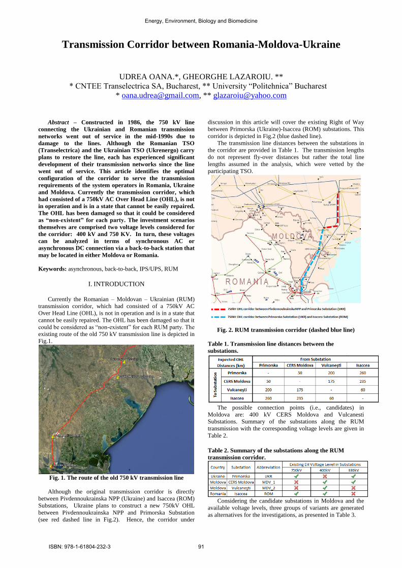
Transmission Corridor between Romania-Moldova-Ukraine

UDREA OANA.*, GHEORGHE LAZAROIU. **

* CNTEE Transelectrica SA, Bucharest, ** University “Politehnica” Bucharest

* [email protected], ** [email protected]

Abstract – Constructed in 1986, the 750 kV line

connecting the Ukrainian and Romanian transmission

networks went out of service in the mid-1990s due to

damage to the lines. Although the Romanian TSO

(Transelectrica) and the Ukrainian TSO (Ukrenergo) carry

plans to restore the line, each has experienced significant

development of their transmission networks since the line

went out of service. This article identifies the optimal

configuration of the corridor to serve the transmission

requirements of the system operators in Romania, Ukraine

and Moldova. Currently the transmission corridor, which

had consisted of a 750kV AC Over Head Line (OHL), is not

in operation and is in a state that cannot be easily repaired.

The OHL has been damaged so that it could be considered

as “non-existent” for each party. The investment scenarios

themselves are comprised two voltage levels considered for

the corridor: 400 kV and 750 KV. In turn, these voltages

can be analyzed in terms of synchronous AC or

asynchronous DC connection via a back-to-back station that

may be located in either Moldova or Romania.

Keywords: asynchronous, back-to-back, IPS/UPS, RUM

I. INTRODUCTION

Currently the Romanian – Moldovan – Ukrainian (RUM)

transmission corridor, which had consisted of a 750kV AC

Over Head Line (OHL), is not in operation and is in a state that

cannot be easily repaired. The OHL has been damaged so that it

could be considered as “non-existent” for each RUM party. The

existing route of the old 750 kV transmission line is depicted in

Fig.1.

Fig. 1. The route of the old 750 kV transmission line

Although the original transmission corridor is directly

between Pivdennoukrainska NPP (Ukraine) and Isaccea (ROM)

Substations, Ukraine plans to construct a new 750kV OHL

between Pivdennoukrainska NPP and Primorska Substation

(see red dashed line in Fig.2). Hence, the corridor under

discussion in this article will cover the existing Right of Way

between Primorska (Ukraine)-Isaccea (ROM) substations. This

corridor is depicted in Fig.2 (blue dashed line).

The transmission line distances between the substations in

the corridor are provided in Table 1. The transmission lengths

do not represent fly-over distances but rather the total line

lengths assumed in the analysis, which were vetted by the

participating TSO.

Fig. 2. RUM transmission corridor (dashed blue line)

Table 1. Transmission line distances between the

substations.

The possible connection points (i.e., candidates) in

Moldova are: 400 kV CERS Moldova and Vulcanesti

Substations. Summary of the substations along the RUM

transmission with the corresponding voltage levels are given in

Table 2.

Table 2. Summary of the substations along the RUM

transmission corridor.

Considering the candidate substations in Moldova and the

available voltage levels, three groups of variants are generated

as alternatives for the investigations, as presented in Table 3.


ISBN: 978-1-61804-232-3 91



Table 3. Substation and voltage level variants to be

investigated.

Initial assumption, was to analyze a total of 36 scenarios

(Substation Variants (4) x Voltage Level Variants (3) x

Seasonal Variants (3) = 36) as given in Table 3. However, the

initial analysis indicated a strong dependency of results to

“Connection Type Variants”. Hence “Connection Type

Variants” are also included in the analysis creating a total of

108 scenarios (108 = 36 x 3 (Connection Type Variants)) to be

analyzed.

II. METHODOLOGY

The approach in load flow and N-1 contingency analysis

will be to search for the maximum amount of power that can be

transferred safely from/to Ukraine+Moldova to/from Romania,

for each combination of Substation and Voltage Level Variants

shown in Table 3. Flowchart of this approach (i.e., algorithm) is

given in Fig. 3. OPF Data of

RUM Countries

Generate Base Case Load Flow Data for Selected

Variant

Set “Exchange

Power = 0” as

Constraint to OPF

Perform OPF

Base Case Security Violations or Convergance

Problems Exist?

Select Next Variant

Perform N-1 Security Analysis

NO

Record Any N-1 Security Violations

Increase Exchange Power

in OPF Constraints

Record the ‘Transmission

Exchange Limit’ for the

Selected Variant

Unhandled Variant Exists?

YES

YES

End of Algorithm

Repeat the Algorithm in Opposite Direction with

Proper Voltage Limit Selection

NOTotal Cost at iteration >

Total Cost at “Exchange Power

= 0”

Record the ‘Market

Exchange Limit’ for

the Selected Variant

YES

Assign or Relax Voltage Limits

Continue with Profit Calculations

Fig. 3. Flow Chart of the methodology (OPF and N-1

contingency analysis)

The reasoning behind “Assign or Relax Voltage Limits”

block can be described as follows: The OPF solution has the

ability to assign voltage constraints for individual buses. At the

data collection phase, the voltage level limits for each RUM

party is collected for high voltage network as given in Table 4.

Table 4. Voltage level limits for analysis.

Voltage constraints are indeed local problems that can be

assumed to be handled by proper operational maneuvers in the

short term (e.g., proper selection of generator voltage set

points) and relatively easy capacitor/reactor investments in the

mid-term. The economical calculations (i.e., cost/benefit

analysis) based on the results with voltage constraints might be

misleading since such voltage problems can be solved either

with reasonable investments in a plausible time frame or with

operational maneuvers in real time). Hence, for long term

decision making analysis, it is more reasonable to work with

OPF results performed ignoring local voltage constraints.

Nevertheless, the OPF and contingency analysis are performed

and results are recorded for both considering and ignoring the

voltage constraints. The effect of voltage constraints on total

generation cost and optimum power exchange amounts in

Scenario 1 is illustrated in Fig. 4, as an example.

Fig. 4. Total generation cost results of Scenario 1 (with and

without voltage constraints).

As illustrated in Fig. 4, the OPF algorithm forces the

solution to a higher cost in order to be able to satisfy the voltage

constraints. The effect is more observable as the exchange

approaches higher values at both directions. However, as the

voltage constraints are relaxed, the cost reduces as OPF does

not consider voltage constraints. The algorithm of the

methodology in Fig. 3 starts from an N-secure case with zero

exchanges and iteratively increases the exchange power through

the RUM corridor in order to find the optimum power exchange

between the parties. The algorithm repeats the followings

iteratively:

Assigns an exchange from/to Ukraine+Moldova

to/from Romania as a constraint to OPF,

Performs an OPF to determine the dispatching,

Compare total generation cost with zero power

exchange case in order to determine the realistic

transaction limit due to price difference,

Creates a load flow scenario based on OPF solution,

Performs N-1 contingency analysis,

Records the N-1 security violations of each scenario,

if any.

Power exchange is increased in 50 MW steps.

The analysis performed with and without voltage

constraints and the results are compared.

Trading scenarios between RUM countries, as predicted by

each party, are given in Table 5. The trading amounts presented

in this table are utilized as “indicative” parameters in the

analysis. As described above, the approach in OPF analysis is

to search for the “maximum” amount of power that can be

transferred N-securely between the RUM countries for each

scenario that are shown in Table 3. In other words, the

algorithm given in Fig. 3 will give the upper limit (i.e.,

maximum) for the N-secure power trading among RUM

countries. The upper limit for the N-secure power trading could

be less or more than the corresponding indicative power

transfer amounts that are shown in Table 5 (last column).

Table 5. Trading scenarios initially predicted by RUM

parties.


ISBN: 978-1-61804-232-3 92

III. COST/BENEFIT ANALYSES

The OPF analyses cover the largest part of the analysis and

create a basis for the cost/benefit analysis which is described in

this section. In this section, performance indicators for

economic and financial analysis, determination of necessary

investments for the corresponding investment scenarios, and

calculation of per unit investment and operation and

maintenance costs are described.

III.1. PERFORMANCE INDICATORS (IRR, NPV, AND B/C

RATIO)

The economic and financial analysis is based on the results

of the OPF analysis, which calculates the total savings to region

at the optimum power exchange in each loading hour (i.e.,

winter max, summer max, and summer min). The Cost/benefit

analysis was made by comparing the results of the OPF analysis

with the investment cost (Inv cost) and operational and

maintenance costs (O&M cost) of the candidate investments.

For each scenario, annual cash flow tables for 30 years

were determined to conduct the following analyses:

Internal rate of return (IRR) analysis,

Net present value (NPV) analysis,

Benefit/Cost ratio (B/C ratio) analysis.

A 30 year useful life of equipment was assumed for the

purposes of the economic/financial calculations. The following

parameters (KEPs) were utilized:

Interest rate of borrowing money for total investment

cost

Loan period

Discount rate for calculating NPVs

The costs of each investment scenario includes:

Total investment cost (TIC) at the initial year (USD),

Annual O&M cost (USD/year).

As described below, annualized savings are considered in

the economic and financial analysis. As described in Section 9,

sensitivity analyses were performed for the key economic

parameters including both AWFs and different generation

levels of wind power plants in Romania.

The year 2012 is considered to be the base year in unit costs

of the equipment. The annual cash flow table is provided in

Table 6.

It should be noted that annual savings can be negative in

some investment scenarios that correspond to the most

constrained loading conditions (e.g., winter max), even during

zero exchange among the countries. This can occur when

voltage constraints combine with high technical losses, and

higher generation levels of the most costly power plants in the

RUM countries than might be dispatched if there was no

interconnection between the RUM countries. The total saving is

assumed to be zero in such cases because the RUM

transmission corridor circuit can be opened to curtail electricity

flow in such circumstances.

Table 6. Annual cash flow table of each scenario.

In the LF and OPF analysis, the maximum savings in each

scenario are determined at three loading hours along the year

(i.e., winter max, summer max, and summer min loading

hours). The savings at these loading hours are utilized in

determining the annual average savings (i.e., annualization of

the savings). Annualization of the savings is based on the

annualized weighting factors (AWF) of these three loading

hours.

The regional system coincident annual hourly load

recordings for 2010 were utilized to determine the AWFs.

Annual hourly coincident regional load and its distribution

along one year are given in Fig. 5 and Fig. 6, respectively. The

following loading hours are indicated in the figures:

System peak (i.e., winter max)

System off-peak (i.e., summer min)

System peak during off-peak season (i.e., summer

max)

Fig. 5. Annual hourly coincident system load

Fig. 5. Distribution of the hourly loads along the year.

AWFs of these three loading hours are indicated in Fig. 6

and summarized in Table 7. Note that, total energy consumed

along the year (the area below the blue curve in Fig. 5) is equal

to (1):

4,29%*(System peak) + 27,58%*(System off-peak) +

68,13%*(System peak during off-peak season) (1)

Table 7. AWFs assumed for RUM countries.


ISBN: 978-1-61804-232-3 93

Loading condition Loading hour AWFs

System peak Winter max 4,29%

System off-peak Summer min 27,58%

System peak during off-peak season

Summer max 68,13%

This approach is analyzed below for the following

parameter and investment scenario (Case_VC-I_W30%):

Investment Scenario No: 1

o 1x400kV Ukraine-MDV_2-ROM

(connection through HVDC B2B substation

at Romania)

Wind generation level at Romania: 30%

Voltage constraints: Ignored

Loading Scenarios:

o Scenario 4: System peak (Winter max)

o Scenario 3: System off-peak (Summer min)

o Scenario 2: System peak during off-peak

season (Summer max)

The savings which are determined by OPF analyses for the

three loading scenarios are given in Table 8.

Table 8. Annualization of savings for the Scenarios 2,3 and

4

As illustrated in the table:

The maximum saving occurs at “system peak” (i.e.,

winter max).

o The room for OPF is maximum given high

generation levels of cost-ineffective power

plants in the region.

The minimum saving occurs at “system off-peak”

(i.e., summer min).

o The potential for optimization is minimal

due to system constraints at minimum

loading conditions

o The availability of cost effective generator

capacity in the system is minimum.

In order to determine the annualized total saving,

availability of the line should be estimated (downtime

for maintenance and unavailability of the line due to

faults must be estimated). An availability of 8322

hours, which corresponds to 95% of the hours in a

year, is assumed for the economic/financial analysis.

Annual saving for this investment scenario is

calculated as 43.596.276,03 USD/year, as illustrated

in Table 8.

This approach was employed in for investment scenarios to

in determine the annualized savings for cost/benefit analysis.

III.2. NECESSARY INVESTMENTS AND CORRESPONDING COSTS

This section reviews the approach to determining the total

amount of equipment that should be installed to support each

investment scenario. The following assumptions are made:

Each substation was equipped with a spare bay at the

corresponding voltage level, in case of

emergency/maintenance/etc.;

750/400 kV or 750/330 kV transformers at the

corresponding substations to satisfy n-1 reliability

criteria;

In the scenarios in which there are two substations in

Moldova, there will be only one transformer in each

substation. This meant that n-1 contingency was

satisfied by the transformer in the other substation;

and

As the intermediary substations in the corridor, the

new substations in Moldova were assumed to have

additional bays- the total number of which depends

on the connection type.

The determination of the necessary equipment for different

investment scenarios is described in the following subsections.

III.2.1. UKRAINE – ROMANIA (1X750 KV AC) In this investment scenario, the following investments are

assumed in Ukraine and Romania:

Primorska/Ukraine:

o Two 750/330 kV transformers (1250 MVA)

o Four 750 kV bay:

One for the transmission line;

Two for the connection of

transformers; and

One for spare.

o Three 330 kV bay:


transformers; and

One for spare.

Isaccea/ Romania:

o Two 750/400 kV transformers (1250

MVA).

o Four 750 kV bay:



transformers; and

One for spare.

o Three 400 kV bay:


transformers; and

One for spare.

The necessary equipment is summarized in Table 9 below.

Table 9. Total amount of equipment necessary for Scenario

1.

III.2.2. UKRAINE – MOLDOVA_1 - ROMANIA (1X750 KV

AC)

Primorska/ Ukraine:

o Two 750/330 kV transformers (1250 MVA)

o Four 750 kV bay:



transformers; and


ISBN: 978-1-61804-232-3 94

One for spare.

o Three 330 kV bay:


transformers; and

One for spare.

CERS Moldova/Moldova:


MVA).

o Five 750 kV bay:

One for the transmission line

input;


output;


transformers; and

One for spare.

o Three 400 kV bay:


transformers; and

One for spare.

Isaccea/Romania:


MVA).

o Four 750 kV bay:



transformers; and

One for spare.

o Three 400 kV bay:


transformers; and

One for spare.


Table 10. Total amount of equipment necessary for

Scenario 2.

III.2.3. UKRAINE – MOLDOVA_1 – MOLDOVA _2 -

ROMANIA (1X750 KV)

Primorska/Ukraine:


MVA).

o Four 750 kV bay:



transformers; and

One for spare.

o Three 330 kV bay:


transformers; and

One for spare.

CERS Moldova/Moldova:

o One 750/400 kV transformer (1250 MVA).

o Four 750 kV bay:


input;


output;

One for the connection of

transformers; and

One for spare.

o Two 400 kV bay:


transformer; and

One for spare.

Vulcanesti/Moldova:

o One 750/400 kV transformer (1250 MVA).

o Four 750 kV bay:


input;


output;


transformer; and

One for spare.

o Two 400 kV bay:


transformers; and

One for spare.

Isaccea/Romania:


MVA).

o Four 750 kV bay:



transformers; and

One for spare.

o Three 400 kV bay:


transformers; and

One for spare.


Table 11. Total amount of equipment necessary for

Scenario 4.


ISBN: 978-1-61804-232-3 95

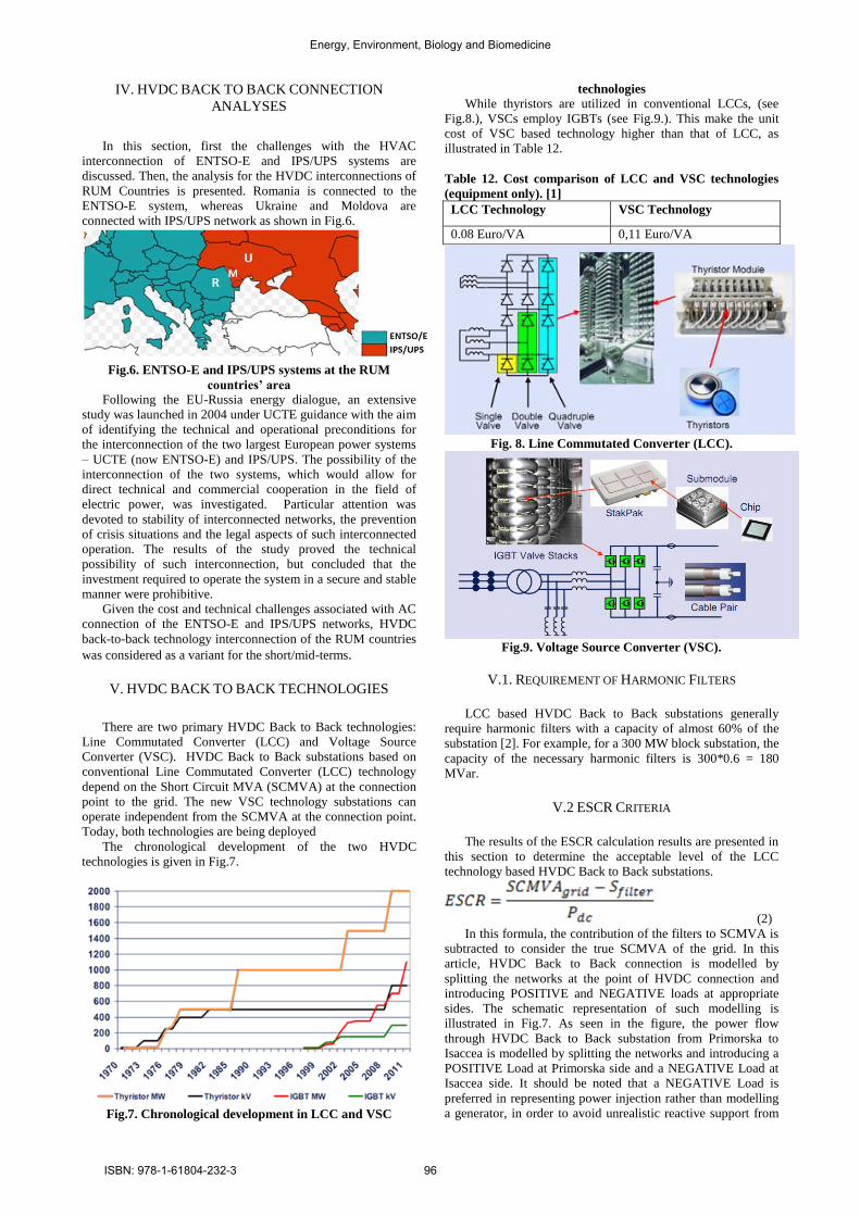
IV. HVDC BACK TO BACK CONNECTION

ANALYSES

In this section, first the challenges with the HVAC

interconnection of ENTSO-E and IPS/UPS systems are

discussed. Then, the analysis for the HVDC interconnections of

RUM Countries is presented. Romania is connected to the

ENTSO-E system, whereas Ukraine and Moldova are

connected with IPS/UPS network as shown in Fig.6.

Fig.6. ENTSO-E and IPS/UPS systems at the RUM

countries’ area

Following the EU-Russia energy dialogue, an extensive

study was launched in 2004 under UCTE guidance with the aim

of identifying the technical and operational preconditions for

the interconnection of the two largest European power systems

– UCTE (now ENTSO-E) and IPS/UPS. The possibility of the

interconnection of the two systems, which would allow for

direct technical and commercial cooperation in the field of

electric power, was investigated. Particular attention was

devoted to stability of interconnected networks, the prevention

of crisis situations and the legal aspects of such interconnected

operation. The results of the study proved the technical

possibility of such interconnection, but concluded that the

investment required to operate the system in a secure and stable

manner were prohibitive.

Given the cost and technical challenges associated with AC

connection of the ENTSO-E and IPS/UPS networks, HVDC

back-to-back technology interconnection of the RUM countries

was considered as a variant for the short/mid-terms.

V. HVDC BACK TO BACK TECHNOLOGIES

There are two primary HVDC Back to Back technologies:

Line Commutated Converter (LCC) and Voltage Source

Converter (VSC). HVDC Back to Back substations based on

conventional Line Commutated Converter (LCC) technology

depend on the Short Circuit MVA (SCMVA) at the connection

point to the grid. The new VSC technology substations can

operate independent from the SCMVA at the connection point.

Today, both technologies are being deployed

The chronological development of the two HVDC

technologies is given in Fig.7.

Fig.7. Chronological development in LCC and VSC

technologies

While thyristors are utilized in conventional LCCs, (see

Fig.8.), VSCs employ IGBTs (see Fig.9.). This make the unit

cost of VSC based technology higher than that of LCC, as

illustrated in Table 12.

Table 12. Cost comparison of LCC and VSC technologies

(equipment only). [1]

LCC Technology VSC Technology

0.08 Euro/VA 0,11 Euro/VA

Fig. 8. Line Commutated Converter (LCC).

Fig.9. Voltage Source Converter (VSC).

V.1. REQUIREMENT OF HARMONIC FILTERS

LCC based HVDC Back to Back substations generally

require harmonic filters with a capacity of almost 60% of the

substation [2]. For example, for a 300 MW block substation, the

capacity of the necessary harmonic filters is 300*0.6 = 180

MVar.

V.2 ESCR CRITERIA

The results of the ESCR calculation results are presented in

this section to determine the acceptable level of the LCC

technology based HVDC Back to Back substations.

(2)

In this formula, the contribution of the filters to SCMVA is

subtracted to consider the true SCMVA of the grid. In this

article, HVDC Back to Back connection is modelled by

splitting the networks at the point of HVDC connection and

introducing POSITIVE and NEGATIVE loads at appropriate

sides. The schematic representation of such modelling is

illustrated in Fig.7. As seen in the figure, the power flow

through HVDC Back to Back substation from Primorska to

Isaccea is modelled by splitting the networks and introducing a

POSITIVE Load at Primorska side and a NEGATIVE Load at

Isaccea side. It should be noted that a NEGATIVE Load is

preferred in representing power injection rather than modelling

a generator, in order to avoid unrealistic reactive support from


ISBN: 978-1-61804-232-3 96

the HVDC Back to Back via the generator. Given this

representation, the SCMVA contribution of the HVDC Back to

Back filters is not considered in the load flow and short circuit

analysis. Therefore, the ESCR should be calculated as in (3).

(3)

For the secure operation of HVDC Back to Back substation

that is based on LCC the

ESCR 3 (base case) [3] (4)

Essentially, the ESCR is different at each connection point

of the HVDC Back to Back substations given different

topologies. For the sake of security, the minimum value among

the SCMVA at each connection point is considered in

calculating of the ESCRs. The available HVDC Back to Back

substation capacity is calculated assuming that total capacity of

the substation is formed by 300 MW blocks, while taking into

account the ESCR criteria (4).

V.3 DETERMINATION OF TOTAL CAPACITY OF HVDC

BACK TO BACK SUBSTATION

It is assumed that the HVDC Back to Back substation

blocks will be in the order of 300 MW capacities. The

following arguments support this approach:

300 MW capacity HVDC Back to Back substations

are available in the market.

The order of 300 MW is plausible to match the

optimum substation capacity with the optimum power

exchange amounts that are determined in LF (Load

Flow) and OPF (Optimal Power Flow) analysis.

For example, the approach in determining the total capacity

of the HVDC Back to Back substation is presented below

(1x400 kV transmission line between Ukraine - Romania

through HVDC Back to Back substation in Ukraine):

Loading condition of the scenario: Summer

maximum.

Wind generation level in Romania: Normal (i.e.,

generation level of the wind power plants in

Dubrudja/ROM region is 30% of the capacity).

OPF results at base case (i.e., ignoring N-1

contingency):

o 700 MW ( Ukraine => Romania)

N-1 security exchange technical limit:

o 1.300 MW ( Ukraine => Romania)

o Since 700 < 1300, 700 MW power

exchange is feasible in the sense of N-1

security concern.

Voltage collapse power exchange limit:

o 1.500 MW ( Ukraine => Romania)

o Since 700 < 1.500, 700 MW power

exchange is feasible in the sense of voltage

collapse concern.

Assuming that HVDC Back to Back substation is

composed of 300 MW blocks, total number of block

to realize 700 MW power exchange is three (3*300 =

900 > 700)

o Total capacity of the HVDC BACK TO

BACK substation is 900 MW.

ESCR criteria:

o Maximum SCMVA of the grid at the

HVDC Back to Back substation is

calculated as 2.063 MVA

o ESCR = 2.063/900 = 2,29

o Since 2,29 < 3, total capacity of 900 MW is

NOT acceptable in the sense of ESCR

criteria.

o If one block among the three blocks is

removed, then the total capacity of the

substation is 2x300 = 600 MW

ESCR = 2.063/600 = 3,43 > 3 =>

acceptable

An HVDC Back to Back capacity of 600 MW is proven in

the summer maximum loading conditions. Similar analyses

were performed for winter maximum and summer minimum

loading conditions, as well. The total capacity of the HVDC

Back to Back substation is considered to be the maximum

capacity determined among three loading scenarios. This

approach is considered in all scenarios that include HVDC

Back to Back substation.

VI. CONCLUSIONS

Voltage constraints were local problems that could be

resolved through network operations in the short term (e.g.,

proper selection of generator voltage set points) and relatively

inexpensive capacitor/reactor investments in the mid-term.

Hence, voltage constraints are ignored in certain cases to

determine the maximum volume of power exchange among the

countries. The maximum voltage deviation at the key nodes

was observed to be +/-20%, which could be resolved by proper

compensation through the provision of additional reactors.

The increase in wind generation in Romania dramatically

limited the ability of the RUM countries to optimize the

regional generation fleet based on the cost of production. In

some investment scenarios, the flow of power changed

direction from north south to south north when the wind

power plant generation in Romania increased from 30% to 70%

and it is designated as must run. This occurs when the OPF

algorithm forced inefficient high cost generators, first in

Romania and then in Moldova and Ukraine, to reduce their

generation in favor of must run wind. This process continued

until the reduction of generation in Ukraine and Moldova

became so much more cost effective than the reduction of

generation in Romania that the power flow changed direction.

From this point onward, Romania began exporting power in a

northward direction to Moldova and Ukraine.

It is important to note that for the investment scenario of a

400 kV connection passing through a HVDC B2B substation,

the benefit/cost ratio was > 1, when Romanian must run wind

generation was modeled with a 30% capacity factor.

Connection through the HVDC Back to Back was superior

to connection through AC options in almost every investment

scenario considered. This was because the HVDC connection

reduced technical network constraints to increase power

exchange, enlarging the scope for power flows in the sub-

region.

In fact, HVDC B2B was the only investment solution which

resulted in benefit/cost > 1 when considering the scenario of

Romanian must run operating with a 30% capacity factor. And,

the technical challenges to synchronizing the current IPS/UPS

and ENTSO-E members of the RUM working group would

inhibit interconnection via high voltage AC interconnections for

the foreseeable future. Therefore, HVDC technology based

interconnection of the RUM countries seemed the most rational

solution in the short/mid-term.

There was no significant difference revealed in the

cost/benefit analyses for the different investment scenarios

related to the configuration of the corridor, i.e., either directly

from Ukraine to Romania or through Moldova. If the

interconnection between RUM countries were realized in

intermediate steps, (for example, if the connection between

Romania and Moldova were realized before all three countries

are interconnected), energy trade between Romania and

Moldova could begin before the trading among all three

countries by directing a generator in Moldova to operate

synchronously with Romania in island mode.


ISBN: 978-1-61804-232-3 97

REFERENCES

[1]. Lazaros P. Lazaridis, “Economic Comparison of HVAC and

HVDC Solutions for Large Offshore Wind Farms under Special

Consideration of Reliability”, Master’s Thesis, Royal Institute

of Technology Department of Electrical Engineering,

Stockholm 2005.

[2]. Dodds, B. Railing, K. Akman, B. Jacobson, T. Worzyk,

“HVDC VSC (HVDC light) transmission – operating

experiences,” CIGRE 2010.

[3]. “Feasibility study of the asynchronous interconnection

between the power systems of Iran and Turkey”, Interim

Report, Professor Francesco Iliceto, Consultant to TEIAS,

Rome (Italy), November 2009.

* Siemens PTI Documentation


ISBN: 978-1-61804-232-3 98

Abstract— To deal with disease, one should distinguish between the normal value and abnormal values related to disease manifestations Beside sign and symptom, biomarkers are among the milstone tools in human disease diagnosis and treatment including strategies for further drug development. Nowadays, there is significant increase in quantitriy and quality of biomarkers used in the process of diagnosis/differential diagnosis, prognosis, treatment decision making and therapy outcomes monitoring. This symposium is aimed to highlight advances and limitations of biomarkers use todate. Biomarkers have an increasingly important clinical role in managing patients with heart failure as well as those with kidney disease, both common conditions with generally poor prognostic outcomes and huge impacts on healthcare economics. For patients with chronic heart failure, biomarkers have become centre place in streamlining diagnostic pathways as well as identifying those with worse prognosis. There is much interest in the role for biomarkers in identifying patients at risk of acute kidney injury, although a number of these currently remain as research tools or are in the early stages of evaluation in clinical practice. Patients with cardiorenal syndrome represent a particular challenge to the clinician, and recent studies have suggested a valuable clinical role for certain biomarkers in this setting, either on their own or in combination. This paper is aimed to highlight advances and limitations of biomarkers use todate focusing on biomarkers with a current clinical role in patients with cardiorenal disease (natriuretic peptides and neutrophil gelatinase-associated lipocalin), although brief reference will be made to other biomarkers with potential future application including those paralleling the drug toxicity.

Keywords—Biomarkers, Diagnosis, Prognosis, Treatment Guide

I. INTRODUCTION

biomarker, or biological marker, generally refers to a measurable characteristic, which may be used

as an indicator of certain biological state or condition. The term occasionally also refers to a substance whose presence indicates the existence or absence of some signs and symptoms in living organisms or a sample drown from. Human physiology is complex and multifactorial and exhibits the properties of a system; where the endocrine system manages metabolism, which is the basis of the continuity of life and the metabolic activity managed by the endocrine system results in the output of biomarkers that reflect the functional achievement of specific aspects of metabolism; while biomarkers are related to each other in ratios, it contextualizes one type of function relative to another to which is it linked anatomically, sequentially, chronologically, biochemically, etc. [1] Thus, biomarkers are used in many scientific fields. Biomarkers in medicine are often measured and evaluated to examine normal biological processes, pathogenic processes, or pharmacologic responses to a therapeutic intervention. In medicine, a biomarker can also be a traceable substance that is introduced into an organism as a means to examine organ function or other aspects of health. For example, rubidium chloride is used as a radioactive isotope to evaluate perfusion of heart muscle. It can also be a substance whose detection indicates a particular disease state, for example, the presence of an antibody may indicate an infection. Before the develpment of dentic testing methods for example

Bimarkers and their utlization in clinical medicine:a contribution to the state of the art

Tesfaye H

A


ISBN: 978-1-61804-232-3 99

only tase of salt of baby meant that the the bayby dies soon at the time care for cystic fibrosis was not so progressive as today. Eventoday the first routine green test for diagnosis of cystic fibrosis is simple sweat-test to estimae the extent of Cl- ions loss in the sweat typycal marker for the gentical disease frequent in caucacian race. More specifically, a biomarker indicates a change in expression or state of a protein that correlates with the risk or progression of a disease, or with the susceptibility of the disease to a given treatment. Biochemical biomarkers are often used in clinical trials, where they are derived from bodily fluids that are easily available to the early phase researchers. A useful way of finding genetic causes of diseases such as schizophrenia has been the use of a special kind of biomarker called an endophenotype. Other biomarkers can be based on measures of the electrical activity of the brain (EEG) or volumetric measures of certain brain regions (using magnetic resonance imaging) or saliva testing of natural metabolites, such as saliva nitrite, a surrogate marker for nitric oxide. Bimarker is generally a molecule that is measured as a marker of normal biological processes, disease processes or the response to a diagnostic or therapeutic intervention. Kidney diseases like acute kidney injury, chronic kidney disease, diabetic nephropathy, glomerular disease, renal cancer and preeclampsia still have a high morbidity. Measurement of biomarkers in the blood or urine that detect patients at risk of kidney diseases or that detect kidney diseases in the earliest stage may ultimately result in preventative or earlier or more effective treatments for kidney diseases. The use of the term "biomarker" has been dated back to as early as 1980. [2] In relevance with its application a biomarker is defined as a characteristic that is objectively measured and evaluated as an indicator of normal biological processes, pathogenic processes, or pharmacologic responses to a therapeutic intervention.[3] Ingeneral, the use of biomarkers to aid diagnosis and treatment is increasing rapidly as genomics and proteomics help us expand the number of markers we can use and as an improved understanding of the pathophysiology of diseases guides their use. However, as with all rapidly expanding fields, there is the risk of excessive enthusiasm unless we are circumspect about the data that guide the clinical use of these new tools. This paper focuses first on

how to use several biomarkers, which at present are the best validated of the new markers, and will hopefully provide insight into how to use this biomarker more productively by distinguishing subsets of patients and by providing an understanding of the meaning of elevations in various clinical situations individually.

FIG. 1. AN IDEAL BIOMARKER SHOULD

INCORPORATE THE CHARACTERSTICS ILLUSTRATED IN THE FIGURE.

II. RENAL MARKERS

Over the past few years and with the use of innovative genomic and proteomic tools, several molecules that their urinary concentration is modified during acute kidney injury have been identified and proposed as biomarkers. Among the most studied biomarkers are neutrophil gelatinase-associated lipocalin-2, kidney injury molecule-1, interleukin-18, cystatin C, N-acetyl-β-D-glucosaminidase, liver fatty-acid binding protein, and heat shock protein 72. Recently review on several existing and recently used renal biomarkers and compared the sensitivity and specificity of each biomarker for the appropriate diagnosis of acute kidney injury, as well as its ability to stratify renal injury and to monitor a renoprotective pharmacologic strategy confirming their importance [5] Acute kidney injury (AKI) has a number of triggers, including ischaemia, nephrotoxins, radiocontrast, and bacterial endotoxins. It occurs in around one-third of patients treated in intensive care


ISBN: 978-1-61804-232-3 100

unit (ICU) and is even more prevalent in cardiac surgery patients. There is a higher mortality in patients with AKI compared with non-AKI counterparts, and in severe AKI requiring renal support, the 6 month mortality is >50%. Unlike the progressive development of biomarkers in cardiology, there have been few changes in kidney diagnostic markers. Creatinine is still used as an indicator of kidney function but not of the parenchymal kidney injury. Serum creatinine (sCr) concentration does not change until around 50% of kidney function is lost, and varies with muscle mass, age, sex, medications, and hydration status. The lag time between injury and loss of function, risks missing a therapeutic opportunity, and may explain the high associated mortality. Novel biomarkers of AKI- and failure include neutrophil gelatinase-associated lipocalin, N-acetyl-β-d-glucosaminidase, kidney injury molecule-1, interleukin-18, and cystatin C. The pathophysiology associated with accumulation of these markers in plasma and urine is not clear, but a common denominator is inflammation. Some of these new AKI biomarkers may have clinical applicability in anaesthesia and intensive care in the future. It is possible that a 'kidney biomarker panel' will become standard before and after major surgery. If elevated or positive, the anaesthetist must take special care to optimize the patients after operation on the surgical wards or ICU to avoid further nephrotoxic insults and initiate supplementary care. [6] Acute kidney injury usually refers to the rapid loss of renal function. In clinical practice, AKI is common among hospitalized patients of all age groups including neonates and remains an important cause of morbidity and mortality due to its late diagnosis and therefore delayed therapeutic intervention. Although the precise incidence of AKI in newborn is unknown, several studies have reported that 8 to 24% of all critically ill newborns in neonatal intensive care units may develop the condition. We aim at reviewing the existing literature on novel serum and urinary biomarkers and discuss their role in the early diagnosis and prognosis of AKI in newborns. Specifically, this review will focus on cystatin C (CysC), neutrophil gelatinase-associated lipocalin (NGAL) and interleukin-18 (IL-18) in serum and on CysC, NGAL, kidney injury molecule-1, and IL-18 in urine. [7] Acute graft dysfunction can be caused by ischaemic damage or

immunological injury leading to serious consequences both in the short and long term. We are in a desperate need for biomarkers of immune and nonimmune injury at different time points of the transplantation time course, beginning from a potential kidney donors where acute kidney damage can pass unnoticed, during the early post-transplant periods to predict acute transplant dysfunction due to various causes and during long term follow up to predict chronic histological changes. The implementation of these novel biomarkers could increase the sensitivity of diagnosis and monitoring of kidney injury in kidney transplant recipients. Traditionally acute graft dysfunction is diagnosed by measuring serum creatinine concentrations. Unfortunately rise in serum creatinine is a late sign of kidney damage. It indicates rather predicts the damage. The treatment, in order to be effective, must be instituted very early after the initiating insult, well before the serum creatinine even begins to rise. Fortunately, emerging technologies such as functional genomics and proteomics have uncovered novel candidates that are emerging as potentially useful biomarkers of acute kidney injury (AKI). The most promising of biomarkers in AKI for clinical use include a plasma panel consisting of Neutrophil Gelatinase-Associated Lipocalin (NGAL) and Cystatin C and a urine panel including NGAL, Il-18 and Kidney Injury Molecule 1 (KIM-1). Most of these biomarkers were developed in non-transplant AKI, yet their role in clinical transplantation has to be identified. [8] Althou heart disease is distinguished organ impairment, it is becoming increasingly recognized that manifestations of congenital heart disease (CHD) extend beyond the cardiovascular system. The factors contributing to renal dysfunction in patients with CHD are multifactorial, with acute kidney injury at time of cardiac surgery playing a major role. Acute kidney injury is often diagnosed based on changes in serum creatinine and estimated glomerular filtration rate (eGFR). Such measurements are often late and imprecise. Recent data indicate that urinary biomarkers interleukin-18 (IL-18) and neutrophil gelatinase-associated lipocalin (NGAL) are earlier markers of AKI. We sought to determine the efficacy of urinary IL-18 and NGAL for detecting early acute kidney injury in patients undergoing surgical pulmonary valve replacement, where both NGAL and IL-18 are


ISBN: 978-1-61804-232-3 101

early predictive biomarkers of acute kidney injury, and both increase in tandem after surgical PVR. Importantly, both rise before an increase in creatinine or a decrease in eGFR is present and it has been concluded that monitoring both biomarkers may allow for earlier detection and subsequent interventions to prevent AKI at time of surgery for CHD.[9] Neutrophil gelatinase-associated lipocalin (NGAL) appears to be a promising biomarker for the early diagnosis of acute kidney injury (AKI); however, a wide range in its predictive value has been reported. Meta-analysis of diagnostic test studies using custom-made standardized data sheets recording plasma/serum and urine NGAL within 6 hours from the time of insult (if known) or 24-48 hours before the diagnosis of acute kidney injury if the time of insult was not known were analysed. The primary outcome was acute kidney injury, defined as an increase in serum creatinine level > 50% from baseline within 7 days or contrast-induced nephropathy (creatinine increase > 25% or concentration > 0.5 mg/dL in adults or > 50% increase in children within 48 hours). Other outcomes predicted using NGAL were renal replacement therapy initiation and in-hospital mortality, and the results using a hierarchical bivariate generalized linear model to calculate the diagnostic odds ratio (DOR) and sample size-weighted area under the curve for the receiver-operating characteristic (AUC-ROC), indicated that NGAL level appears to be of diagnostic and prognostic value for acute kidney injury. [10] The early detection of acute kidney injury (AKI) may be become possible by several promising early biomarkers which may facilitate the early detection, differentiation and prognosis prediction of AKI. In this study, we investigated the value of urinary liver-type fatty acid-binding protein (L-FABP), neutrophil gelatinase-associated lipocalin (NGAL) and their combination in predicting the occurrence and the severity of AKI following cardiac surgery. Urinary L-FABP and NGAL increased at an early stage after cardiac surgery indicating that the combination of the two biomarkers enhanced the accuracy of the early detection of postoperative acute kidney injury after cardiac surgery before a rise in SCr. [11]. In some conditions related to exposure to nephrotoxic drugs like aminoglycosides and glycopeptides antibiotics ,

ofcourse the most guding biomarker may be elevation of serum creatinine level.[12], [13] In rare circumstances serum creatinine may paradoxically decline so that one may overlook the underlying renal toxicity hanging on low serum creatinine level, unless the drug level is promptely monitored.[14] Therefore, serum creatinine should carefully evaluated within the context of state of hydration, underlying disease, and nephrotoxic agents exposure in the past or at present.

III. LIVER BIOMARKERS Liver as the largest metabolically active organ has its own relatively specific biomarkers regarding acute and chronic isults or toxic injury. Serum bilirubin level and several enzaymes including aminotrasferases are used to assess liver cells integrity. Albumin and other liver products can also mark liver fucinal or ysynthetic capacity state. The liver markers mybe associated also with extrahepaic disorders requiring careful interpretation.

Table 1. Short summary of some liver biomarkers and their localization

IV. CURRENTLY USEDCARDIAC SPECIFIC BIOMARKERS

Despite better establishment of currently used cardiac-specific serum markers unfortunately non- meets all the criteria for an "ideal" marker of acute myocardial infarction (AMI). No test is both highly


ISBN: 978-1-61804-232-3 102

sensitive and highly specific for acute infarction within 6 hours following the onset of chest pain, the timeframe of interest to most emergency physicians in making diagnostic and therapeutic decisions. Patients presenting to the emergency departments (ED) with chest pain or other symptoms suggestive of acute cardiac ischemia therefore cannot make a diagnosis of AMI excluded on the basis of a single cardiac marker value obtained within a few hours after symptom onset. The total CK level is far too insensitive and nonspecific a test to be used to diagnose AMI. It retains its value, however, as a screening test, and serum of patients with abnormal total CK values should undergo a CK-MBmass assay. Elevation in CK-MB is a vital component of ultimate diagnosis of AMI, but levels of this marker are normal in one fourth to one half of patients with AMI at the time of ED presentation. The test is highly specific, however, and an abnormal value (particularly when it exceeds 5% of the total CK value) at any time in a patient with chest pain is highly suggestive of an AMI. There have been several improvements of CK-MB assay timing and subform quantification that appear highly useful for emergency physicians. Rapid serial CK-MB assessment greatly increases the diagnostic value of the assay in a timeframe suitable for ED purposes but unfortunately still misses about 10% of patients ultimately diagnosed with acute MI. Assays of CK-MB subforms have very high sensitivity, and, although unreliable within 4 hours of symptom onset, have excellent diagnostic value at 6 or more hours after chest pain begins. Automated test assays recently have become available and could prove applicable to ED settings. The cardiac troponins are highly useful as markers of acute coronary syndromes, rather than specifically of AMI, and abnormal values at any time following chest pain onset are highly predictive of an adverse cardiac event. The ED applicability of the troponins is severely limited, however, because values remain normal in most patients with acute cardiac events as long as 6 hours following symptom onset. Myoglobin appeared promising as a marker of early cardiac ischemia but appears to be only marginally more sensitive than CK-MB assays early after symptom onset and less sensitive than CK-MB at 8 hours or more after chest pain starts. Rapid serial myoglobin assessment, however, appears highly useful as an early marker of AMI. The marker has a

very narrow diagnostic window. The clinician is left with several tests that are highly effective in correctly identifying patients with AMI (or at high risk for AMI), but none that can dependably exclude patients with acute coronary syndromes soon after chest pain onset. A prudent strategy when assessing ED patients with chest pain and nondiagnostic ECGs is to order CK-MB and troponin values on presentation in the hope of making an early diagnosis of AMI or unstable coronary syndrome. Although it is recognized that normal values obtained within 6 hours of symptom onset do not exclude an acute coronary syndrome, patients at low clinical risk and having normal cardiac marker tests could be provisionally admitted to low-acuity hospital settings or ED observation. After 6 to 8 hours of symptom duration has elapsed, the cardiac-specific markers are highly effective in diagnosing AMI, and such values obtained can be used more appropriately to make final disposition decisions. At no time should results of serum marker tests outweigh ECG findings or clinical assessment of the patient's risk and stability.[15] Biochemical markers provide clinicians with an important tool for the assessment of acute coronary syndromes. Biochemical markers, including total creatine kinase (total CK), creatine kinase-MB (CK-MB), the MB isoforms, and myoglobin, as well as the troponins--cardiac troponin T (cTnT) and cardiac troponin I (cTnI)--are all used for assessment of the suspected acute myocardial infarction (AMI) patient. In the context of myocardial infarction (MI) diagnosis, total CK is a relatively sensitive marker, but it lacks myocardial specificity because skeletal muscle contains high concentrations of CK. CK-MB is the benchmark for biochemical markers and has both high sensitivity and specificity; however, CK-MB is also present in skeletal muscle and is not diagnostic until eight to twelve hours after onset of symptoms. The MB isoforms are diagnostic earlier but have the same cardiac specificity issues as CK-MB. Myoglobin becomes abnormal about one hour after onset of symptoms and is a sensitive marker for MI; however, myoglobin is cleared quickly and is not cardiac specific. Furthermore myglobin together with CK may be significantly elevated in association to some drug overdose leading severe hypokalaemia leading to lifethreatening arrhythmia. [16] Both cTnT and cTnI are cardiac specific and


ISBN: 978-1-61804-232-3 103

show high sensitivity and specificity for MI. Risk stratification of acute coronary syndrome patients is another role for biochemical markers; CK-MB, cTnT and cTnI have all been proposed for this function. Compared with CK-MB, both cTnT and cTnI are better able to predict short-term mortality following the index event. Analysis using a logistic regression model that included the electrocardiogram, cTnT, and cTnI showed that cTnT is the most useful marker for risk stratification and cTnT was reported to be able to predict which patients will benefit from treatment with regimens of low molecular weight heparin. [17] In the past decade studies have suggested that immunoassay of cardiac troponin T (cTnT) provides a more sensitive measurement of myocardial necrosis than creatine kinase MB (CK-MB) mass concentration. Abbas et al. who, compared the release of cTnT and CK-MB isoenzyme in patients undergoing percutaneous coronary angioplasty, and investigated the clinical, procedural, and angiographic correlates of abnormal elevations of both of these markers concluded that > 40% of patients undergoing coronary angioplasty have evidence of minor degrees of myocardial damage, as evidenced by cTnT release. Thus, high-risk coronary lesions and both minor and major complications of angioplasty are associated with cTnT release. cTnT appears to be a more sensitive marker of myocardial injury than CK-MB under these circumstances. In comparison with isolated cTnT rise, elevation of both CK-MB and cTnT may be indicative of greater levels of myocardial injury. [18] Variable degrees of myocardial cell injury during PTCA and stent insertion have been observed, based on rises in creatine kinase MB isoenzyme (CK-MB) and cardiac troponin T (cTnT) 6-24 h post-procedure. As there are many variations in technique within each procedure it would be helpful to be able to determine objectively the degree of myocardial damage in order to optimize technique. Harris et al. who measured CK-MB, cTnT and cardiac troponin I (cTnI) to ascertain which is the most sensitive marker for minor myocardial damage in this setting demonstrated that cTnI was the most sensitive indicator of minor myocardial damage. [19] In the study performed to determine the most sensitive biochemical marker for the detection of cardiac myocyte damage potentially sustained during percutaneous coronary intervention (PCI) and to assess whether such a

marker can be used to identify patients at increased risk of poor subsequent clinical outcome, Nageh et al. revealed that cTnI proved to be the most sensitive marker in detecting myocardial necrosis following PCI. CK-MB, cTnT and cTnI all provided similarly reliable prognostic information, with cTnT and cTnI being marginally superior in predicting MACE at follow up. [20] The explosion in cardiovascular biomarkers has been stimulated in large part by proteomics, genomics and an improved understanding of the pathophysiology of cardiovascular disease. In the past few years, major changes have evolved in clinicians‘ ability to use cardiac troponin, BNP and CRP which will markedly impact on their clinical utility. The recent changes including greater sensitivity, a better understanding of what specific fragments are being measured and now these markers are used clinically as obligatory, but the search for better markers must continue. [21] Jaffe et al discussed the use of troponin as well as the knowledge gaps associated with emerging biomarkers such as B-type natriuretic peptide and C-reactive protein, which are increasingly moving toward more productive clinical use and reflected on some of the large number of markers that are still in development. [22] The prognostic significance of elevations in creatine kinase-MB and troponin T (cTnT), which have been conventionally measured 6 to 8 h after percutaneous coronary intervention (PCI), has been established. but, the time to peak biomarker appearance in the circulation has not been well defined. Later studey revealed that more cTnT than CK-MB elevations occur after PCI; however, both biomarkers demonstrate a longer time to peak value than anticipated in clinical practice. Early surveillance monitoring (< 12 h) does not detect peak biomarker levels, especially in patients with normal baseline values. If peak levels are to be used to determine prognosis, then longer time intervals should be used for post-PCI surveillance. The timing of peak elevations appears to be influenced by baselines values as well. Early elevations may reflect the conjoint effects of injury associated with the disease process and the intervention itself. [23] The adverse prognostic significance of biomarker elevations after percutaneous coronary intervention (PCI) is well established. However, often baseline troponin values are not included in the analysis or sensitive criteria are not employed till Miller et al.


ISBN: 978-1-61804-232-3 104

assessed the timing and magnitude of post-PCI troponin T (cTnT) levels and their relationships to outcomes in patients with and without pre-PCI baseline cTnT elevations using a sensitive assay and sensitive cut-off values and finally revealed that long-term prognosis is most often related to the baseline pre-PCI troponin value and not the biomarker response to the PCI.[24]

V. EARLY NEURON DAMGE BIOMARKERS

Severe brain disorders can be expressed as markedly abnormal encephalopathic EEG patterns in neonates who are usually neurologically depressed, with abnormal levels of reactivity and tone. EEG sleep study can serve as a useful neurophysiologic screening procedure for the child suspected of having a subclinical presentation of an emerging static encephalopathy; longitudinal studies will then document deviations from expected ontogeny in the vulnerable child who is later stressed by environmental and socioeconomic factors. [25] Encephalopathy consequent on perinatal hypoxia-ischemia occurs in a number of newborns and frequently leads to serious and tragic consequences that devastate lives and families, with huge financial burdens for society. Brain pH changes are closely involved in the control of cell death after injury: an alkalosis enhances excitability while a mild acidosis has the opposite effect. Brain alkalosis in babies with neonatal encephalopathy serially studied using phosphorus-31 magnetic resonance spectroscopy studies during the first year after birth (151 studies throughout the year including 56 studies of 50 infants during the first 2 weeks after birth) proved that an alkaline brain pH was associated with severely impaired outcome; the degree of brain alkalosis was related to the severity of brain injury on MRI and brain lactate concentration; and a persistence of an alkaline brain pH was associated with cerebral atrophy on MRI. [26] Although intenssive fetal and neonatal resuscitative efforts have reduced the severe expression of the neonatal brain disorder termed hypoxic-ischemic encephalopathy, neonates may alternatively express altered EEG-sleep organization over the first days of life after asphyxia which may mimic mild or moderate hypoxic-ischemic encephalopathy. EEG-sleep studies can assist in a more accurate classification of newborn

encephalopathy that does not satisfy the criteria for hypoxic-ischemic encephalopathy. [27] Hypoxic ischemic encephalopathy after perinatal asphyxia is a major cause of mortality and morbidity in infants. Asphyxiated infants displayed neuronal cell damage and reactive glial changes with strong aquaporin-4 immunoreactivity on astroglial cells within hippocampi in 50% of cases, whereas in patients with seizures, the expression of metabotropic glutamate receptors was increased in glial cells, where cases with seizures displayed increased microglial activation and greater expression of the inflammatory markers interleukin 1β and complement 1q compared with those in cases without seizures confirming the complex cascade of cellular and molecular changes occurring in the human neonatal hippocampus after perinatal asphyxia. [28] Anticonvulsant therapy has been used in infants with perinatal asphyxia in order to prevent seizures. However, long term anticonvulsant therapy may lead to inhibition of brain development. Therefore, the routine use of anticonvulsant therapy to prevent seizures following perinatal asphyxia needs to be evaluated. At the present time, anticonvulsant therapy to term infants in the immediate period following perinatal asphyxia cannot be recommended for routine clinical practice, other than in the treatment of prolonged or frequent clinical seizures. Any future studies should be of sufficient size to have the power to detect clinically important reductions in mortality and severe neurodevelopmental disability. [29]

VI. CANCER BIOMARKERS

Among pioners in the biomarker area of malignant (cancer) diseases, alpha-fetoprotein (AFP) is a well-known diagnostic biomarker used in medicine to detect fetal developmental anomalies such as neural tube defects or Down’s syndrome is also used to date to follow up the development of tumors such as hepatocellular carcinomas todate since its discovery more than half a century ago. [30] Tumor markers in general are endogenous proteins or metabolites whose amounts or modifications are indicative of tumor state, progression characteristics, and response to therapies. They are present in tumor tissues or body fluids and encompass a wide variety of molecules, including


ISBN: 978-1-61804-232-3 105

transcription factors, cell surface receptors, and secreted proteins. Effective tumor markers are in great demand since they have the potential to reduce cancer mortality rates by facilitating diagnosis of cancers at early stages and by helping to individualize treatments. During the last decade, improved understanding of carcinogenesis and tumor progression has revealed a large number of potential tumor markers. It is predicted that even more will be discovered in the near future with the application of current technologies such as tissue microarrays, antibody arrays, and mass spectrometry. To apply these discoveries to patient care, vigorous validation and assay development for many tumor markers is currently underway. The reason behind so few biomarkers reaching the clinic can largely be explained by the inability of current technologies to consistently and quantitatively verify the presence of the candidates in patient samples and the failure, thus far, to identify biomarkers with high specificity for a particular disease as some times none of the cancer biomarkers demonstrate the specificity required for diagnosis when used alone. Therefore, the development of panels of proteins further may be crucial to achieve the specificity required for early cancer diagnosis, and is interesting to speculate that members of such panels are likely to have already been identified but not yet implemented. [31] A There were study results confirming that the combination of age at onset and tumor phenotype can provide an efficient model for identifying individuals with a high probability of carrying BRCA mutations and supporting the hypothesis that breast cancer in BRCA carriers is qualitatively distinct from other early-onset breast cancers and from late-onset, sporadic, breast carcinomas.[32] Tumors with mutations in the gene encoding the serine-threonine protein kinase BRAF are dependent on the MAPK signaling pathway for their growth, what offers an opportunity to test oncogene-targeted therapy. Mutations at the position V600 of BRAF were described in approximately 8% of all solid tumors, including 50% of melanomas, 30 to 70% of papillary thyroid carcinomas and 5 to 8% of colorectal adenocarcinomas. Specific BRAF kinase inhibitors are undergoing rapid clinical development and promising data on efficacy have been demonstrated in activated mutant BRAF V600 melanomas. This

review article will address: (a) preclinical data on the antitumor activity of BRAF inhibitors in cell lines/ in vivo models and their opposing functions [33] The advent of targeted therapies has revolutionized the treatment of certain types of cancer. Identification of molecular targets on cancer cells has led to the design of novel drugs, which either used as single agents or in combination with chemotherapy, has prolonged survival in metastatic disease, or contributed to curative treatment in the adjuvant setting. A literature review was conducted to identify and present current knowledge on the molecular function of the HER2 receptor, its role in the pathogenesis of breast cancer and anti-HER2 targeted drugs in use or under development. Many molecular targets have been identified in breast cancer, with the HER family of receptors being the ones most extensively studied [34] There was published study results suggest that circulating plasma sKIT levels seem to function as a surrogate marker for TTP in gastrointestinal stromal tumor patients although additional studies are warranted to confirm and expand these findings[35] According to some study, it is reasonable to suggest that PSA density, velocity, doubling time and free to total PSA ratio or combining PSA with Gleason score shall greatly increase PSA specificity in detecting PC cases. Radioisotopic bone scan by SPET or PET can demonstrate osseous metastases at later stages of PC, but should also be applied in cases falsely considered as an early stage of PC, for better staging and for periodic follow-up of the disease. [36] The protein S-100B seems to be the best analyzed biomarker in melanoma and tt has the potential to identify high-risk stage III melanoma patients who may benefit from adjuvant systematic treatment. Since an effective (adjuvant) therapy for loco-regional metastatic and disseminated melanoma is recently introduced, the use of S-100B seems to alter dramatically in the near future [37] Despite advances in genomics, proteomics and molecular pathology have generated many candidate biomarkers with potential clinical value, their use for cancer staging and personalization of therapy at the time of diagnosis could improve patient care. The challenge of translation from bench to bedside outside of the research setting has proved more difficult than might have been expected. Thus, understanding how and when


ISBN: 978-1-61804-232-3 106

biomarkers can be integrated into clinical care is crucial if to translate the promise into reality as repoted already. [38] Biomarkers present the normal and/or disease state in humans. Genetic and epigenetic biomarkers assessed in easily accessible biological materials are useful in diagnosis, early onset or risk of developing cancer or to predict the treatment efficacy or clinical outcome of different human malignancies. Some of these markers are also expressed during early stages of the tumor development and hence provide an opportunity to develop intervention and treatment strategies. Withthe advances of research in clinical genetic and epigenetic, once validated, these markers can be utilized in clinical settings and to identify high risk populations through their implication in cancer diagnosis and risk assessment. [39] Tissue inhibitor of metalloproteinase-1 (TIMP-1) was evaluated in the pre-treatment serum of newly diagnosed patients with symptomatic myeloma and revealed that pre-treatment serum TIMP-1 is associated with advanced myeloma suggestsing further evaluation of this molecule to better determine its prognostic potential in MM. [40] Significant number of metastases from hormone receptor-positive primary breast cancer do not respond to endocrine therapy. A study to assess how often hormone receptor status changes between primary and recurrent tumors and whether such a change might explain unresponsiveness to endocrine therapy indicated that loss of estrogen receptor (ER) expression in recurrent breast cancer should be considered as a cause for poor response to endocrine therapy in primarily ER-positive patients. [41] According to a review from thirteen categories of breast tumor markers considered, not all applications for these markers were supported due some demonstrated insufficient evidence to support routine use in clinical practice [42] The therapeutic strategy for breast cancer with the use of targeted drugs is, at present, mainly focused on coping with HER2 as currently for instance lapatinib and trastuzumab are in widespread use. [43] Treatment decisions for patients with lung cancer have historically been based on tumour histology. Mutations in EGFR and KRAS have been extensively studed, but the application of treatment according to the genetic potential of individual tumours may lead to substantial therapeutic improvements as stated in recent review. [44] The tissue concentrations of

specific miRNAs have been associated with tumor invasiveness, metastatic potential, and other clinical characteristics for several types of cancers, including chronic lymphocytic leukemia, and breast, colorectal, hepatic, lung, pancreatic, and prostate cancers. The biologic roles of miRNAs in cancer also suggest a correlation with prognosis and therapeutic outcome indicating further investigation of these roles to lead to new approaches for the categorization, diagnosis, and treatment of human cancers. [45]

Table 2. Breif list of some molecular cancer biomarkers

Beyound the breif list above, other examples of biomarkers also include: Tumor suppressors lost in cancer (Examples: BRCA1, BRCA2), RNA (Examples: mRNA, microRNA), and proteins found in body fluids or tissue like prostate-specific antigen, and CA-125). [46]

VII. CONCLUSION

Today we have several biomarkers used in major fields and specialities of medicine. These are not only to help disease diagnosis and differential diagnosis, also to develope new drugs to target certain pathologies and to rationally use treatment measures available at the right time for the right patient. Keeping on utilizing the well established markers, we can also develope the newer and more sensitive and specific ones based on the present knowledge deepening supported by further clinical application and evidences collected from multicentere settings.


ISBN: 978-1-61804-232-3 107

http://en.wikipedia.org/wiki/BRCA1

http://en.wikipedia.org/wiki/BRCA2

http://en.wikipedia.org/wiki/MRNA

http://en.wikipedia.org/wiki/MicroRNA

http://en.wikipedia.org/wiki/Prostate-specific_antigen

http://en.wikipedia.org/wiki/Prostate-specific_antigen

http://en.wikipedia.org/wiki/CA-125

conclusion section is not required. Although a conclusion may review the main points of the paper, do not replicate the abstract as the conclusion. A conclusion might elaborate on the importance of the work or suggest applications and extensions.

REFERENCES

[1]. LAPRAZ JC, HEDAYAT KM, PAULY P. ENDOBIOGENY: A GLOBAL APPROACH TO SYSTEMS BIOLOGY (PART 2 OF 2). GLOB ADV HEALTH MED.

2013;2:32-44.

[2]. Aronson J. Biomarkers and surrogate endpoints. British Journal of Clinical Pharmacology 2005; 59 : 491–494

[3]. Biomarkers Definitions Working Group. Biomarkers and surrogate endpoints: preferred definitions and conceptual framework. Clinical Pharmacology & Therapeutics 2001; 69: 89–95.

[4]. Strimbu, K, Jorge T. What are Biomarkers? Current Opinion in HIV and AIDS 2010;5 : 463–466.

[5]. Barrera-Chimal J, Bobadilla NA. Are recently reported biomarkers helpful for early and accurate diagnosis of acute kidney injury? Biomarkers 2012; 17:385-93

[6]. Mårtensson J, Martling CR, Bell M. Novel biomarkers of acute kidney injury and failure: clinical applicability. Br J Anaesth. 2012;109:843-50 [7]. Argyri I, Xanthos T, Varsami M, Aroni F, Papalois A, Dontas I, Fanos V, Iacovidou N.The role of novel biomarkers in early diagnosis and prognosis of acute kidney injury in newborns. Am J Perinatol. 2013;30:347-52 [8]. Halawa A. The early diagnosis of acute renal graft dysfunction: a challenge we face. The role of novel biomarkers. Ann Transplant. 2011;16:90-8 [9]. Buelow MW, Dall A, Regner K, Weinberg C, Bartz PJ, Sowinski J, Rudd N, Katzmark L, Tweddell JS, Earing MG.Urinary interleukin-18 and urinary neutrophil gelatinase-associated lipocalin predict acute kidney injury following pulmonary

valve replacement prior to serum creatinine. Congenit Heart Dis. 2012;7:441-7. [10]. Haase M, Bellomo R, Devarajan P, Schlattmann P, Haase-Fielitz A; NGAL Meta-analysis Investigator Group. Accuracy of neutrophil gelatinase-associated lipocalin (NGAL) in diagnosis and prognosis in acute kidney injury: a systematic review and meta-analysis. Am J Kidney Dis. 2009;54:1012-24 [11]. Liu S, Che M, Xue S, Xie B, Zhu M, Lu R, Zhang W, Qian J, Yan Y. Urinary L-FABP and its combination with urinary NGAL in early diagnosis of acute kidney injury after cardiac surgery in adult patients. Biomarkers. 2013;18:95-101 [12]. Tesfaye H., Jedličková B., Průša R. Evidence of renal function deterioration on once-daily administration of amikacin in an elderly patient: a warning case Klin. Biochem. Metab., 2007;15: 49–52 [13]. Tesfaye H, Lukášková J, Hořínková J.Sudden renal function deterioration in an elderly patient on vancomycin therapy for endocarditis. Cas Lek Cesk 2012;151:531-4 [14]. Tesfaye H., Průša R., Kolařova J., Šimonek J., Lischke R. Rapid decline of serum creatinine and a challenge of aminoglycoside dosing: a case of post bilateral lung transplantation cystic fi brosis patient Klin. Biochem. Metab;2009, 17: 256–259

[15]. Karras DJ, Kane DL. Serum markers in the emergency department diagnosis of acute myocardial infarction. Emerg Med Clin North Am. 2001;19:321-37

[16]. Tesfaye H, Průsa R, Doupovcová J. Hypokalaemia in a suicide attempt of an adolescent girl. Cas Lek Cesk 2008;147:333-6

[17]. Christenson RH, Newby LK, Ohman EM. Cardiac markers in the assessment of acute coronary syndromes. Md Med J. 1997;Suppl:18-24

[18]. Abbas SA, Glazier JJ, Wu AH, Dupont C, Green SF, Pearsall LA, Waters DD, McKay RG. Factors associated with the release of cardiac troponin T following percutaneous transluminal coronary angioplasty. Clin Cardiol. 1996;19:782-6.

[19]. Harris BM, Nageh T, Marsden JT, Thomas MR, Sherwood RA. Comparison of cardiac troponin


ISBN: 978-1-61804-232-3 108

http://www.ncbi.nlm.nih.gov/pubmed?term=M%C3%A5rtensson%20J%5BAuthor%5D&cauthor=true&cauthor_uid=23048068

http://www.ncbi.nlm.nih.gov/pubmed?term=Martling%20CR%5BAuthor%5D&cauthor=true&cauthor_uid=23048068

http://www.ncbi.nlm.nih.gov/pubmed?term=Bell%20M%5BAuthor%5D&cauthor=true&cauthor_uid=23048068

http://www.ncbi.nlm.nih.gov/pubmed?term=Argyri%20I%5BAuthor%5D&cauthor=true&cauthor_uid=23023560

http://www.ncbi.nlm.nih.gov/pubmed?term=Xanthos%20T%5BAuthor%5D&cauthor=true&cauthor_uid=23023560

http://www.ncbi.nlm.nih.gov/pubmed?term=Varsami%20M%5BAuthor%5D&cauthor=true&cauthor_uid=23023560

http://www.ncbi.nlm.nih.gov/pubmed?term=Aroni%20F%5BAuthor%5D&cauthor=true&cauthor_uid=23023560

http://www.ncbi.nlm.nih.gov/pubmed?term=Papalois%20A%5BAuthor%5D&cauthor=true&cauthor_uid=23023560

http://www.ncbi.nlm.nih.gov/pubmed?term=Dontas%20I%5BAuthor%5D&cauthor=true&cauthor_uid=23023560

http://www.ncbi.nlm.nih.gov/pubmed?term=Fanos%20V%5BAuthor%5D&cauthor=true&cauthor_uid=23023560

http://www.ncbi.nlm.nih.gov/pubmed?term=Iacovidou%20N%5BAuthor%5D&cauthor=true&cauthor_uid=23023560

http://www.ncbi.nlm.nih.gov/pubmed/23023560



http://www.ncbi.nlm.nih.gov/pubmed?term=Halawa%20A%5BAuthor%5D&cauthor=true&cauthor_uid=21436782


http://www.ncbi.nlm.nih.gov/pubmed?term=Buelow%20MW%5BAuthor%5D&cauthor=true&cauthor_uid=22537138

http://www.ncbi.nlm.nih.gov/pubmed?term=Dall%20A%5BAuthor%5D&cauthor=true&cauthor_uid=22537138

http://www.ncbi.nlm.nih.gov/pubmed?term=Regner%20K%5BAuthor%5D&cauthor=true&cauthor_uid=22537138

http://www.ncbi.nlm.nih.gov/pubmed?term=Weinberg%20C%5BAuthor%5D&cauthor=true&cauthor_uid=22537138

http://www.ncbi.nlm.nih.gov/pubmed?term=Bartz%20PJ%5BAuthor%5D&cauthor=true&cauthor_uid=22537138

http://www.ncbi.nlm.nih.gov/pubmed?term=Sowinski%20J%5BAuthor%5D&cauthor=true&cauthor_uid=22537138

http://www.ncbi.nlm.nih.gov/pubmed?term=Rudd%20N%5BAuthor%5D&cauthor=true&cauthor_uid=22537138

http://www.ncbi.nlm.nih.gov/pubmed?term=Katzmark%20L%5BAuthor%5D&cauthor=true&cauthor_uid=22537138

http://www.ncbi.nlm.nih.gov/pubmed?term=Tweddell%20JS%5BAuthor%5D&cauthor=true&cauthor_uid=22537138

http://www.ncbi.nlm.nih.gov/pubmed?term=Earing%20MG%5BAuthor%5D&cauthor=true&cauthor_uid=22537138


http://www.ncbi.nlm.nih.gov/pubmed?term=Haase%20M%5BAuthor%5D&cauthor=true&cauthor_uid=19850388

http://www.ncbi.nlm.nih.gov/pubmed?term=Bellomo%20R%5BAuthor%5D&cauthor=true&cauthor_uid=19850388

http://www.ncbi.nlm.nih.gov/pubmed?term=Devarajan%20P%5BAuthor%5D&cauthor=true&cauthor_uid=19850388

http://www.ncbi.nlm.nih.gov/pubmed?term=Schlattmann%20P%5BAuthor%5D&cauthor=true&cauthor_uid=19850388

http://www.ncbi.nlm.nih.gov/pubmed?term=Haase-Fielitz%20A%5BAuthor%5D&cauthor=true&cauthor_uid=19850388

http://www.ncbi.nlm.nih.gov/pubmed?term=NGAL%20Meta-analysis%20Investigator%20Group%5BCorporate%20Author%5D

http://www.ncbi.nlm.nih.gov/pubmed?term=NGAL%20Meta-analysis%20Investigator%20Group%5BCorporate%20Author%5D


http://www.ncbi.nlm.nih.gov/pubmed?term=Liu%20S%5BAuthor%5D&cauthor=true&cauthor_uid=23167703

http://www.ncbi.nlm.nih.gov/pubmed?term=Che%20M%5BAuthor%5D&cauthor=true&cauthor_uid=23167703

http://www.ncbi.nlm.nih.gov/pubmed?term=Xue%20S%5BAuthor%5D&cauthor=true&cauthor_uid=23167703

http://www.ncbi.nlm.nih.gov/pubmed?term=Xie%20B%5BAuthor%5D&cauthor=true&cauthor_uid=23167703

http://www.ncbi.nlm.nih.gov/pubmed?term=Zhu%20M%5BAuthor%5D&cauthor=true&cauthor_uid=23167703

http://www.ncbi.nlm.nih.gov/pubmed?term=Lu%20R%5BAuthor%5D&cauthor=true&cauthor_uid=23167703

http://www.ncbi.nlm.nih.gov/pubmed?term=Zhang%20W%5BAuthor%5D&cauthor=true&cauthor_uid=23167703

http://www.ncbi.nlm.nih.gov/pubmed?term=Qian%20J%5BAuthor%5D&cauthor=true&cauthor_uid=23167703

http://www.ncbi.nlm.nih.gov/pubmed?term=Yan%20Y%5BAuthor%5D&cauthor=true&cauthor_uid=23167703


T and I and CK-MB for the detection of minor myocardial damage during interventional cardiac procedures. Ann Clin Biochem. 2000;37 ( Pt 6):764-9.

[20]. Nageh T, Sherwood RA, Harris BM, Byrne JA, Thomas MR. Cardiac troponin T and I and creatine kinase-MB as markers of myocardial injury and predictors of outcome following percutaneous coronary intervention. Int J Cardiol. 2003;92:285-93

[21]. Jaffe AS. Cardiovascular biomarkers: the state of the art in 2006. Clin Chim Acta. 2007;381:9-13.

[22]. Jaffe AS, Babuin L, Apple FS. Biomarkers in acute cardiac disease: the present and the future. J Am Coll Cardiol. 2006;48:1-11.

[23]. Miller WL, Garratt KN, Burritt MF, Reeder GS, Jaffe AS. Timing of peak troponin T and creatine kinase-MB elevations after percutaneous coronary intervention. Chest 2004 ;125:275-80.

[24]. Miller WL, Garratt KN, Burritt MF, Lennon RJ, Reeder GS, Jaffe AS. Baseline troponin level: key to understanding the importance of post-PCI troponin elevations. Eur Heart J. 2006 ;27:1061-9.

[25]. Scher MS. Neurophysiological assessment of brain function and maturation. II. A measure of brain dysmaturity in healthy preterm neonates. Pediatr Neurol. 1997;16:287-9

[26]. Uria-Avellanal C, Robertson NJ. Na(+)/H (+) Exchangers and Intracellular pH in Perinatal Brain Injury. Transl Stroke Res. 2014;5:79-98.

[27]. Scher MS, Steppe DA, Beggarly ME, Salerno DG, Banks DL Neonatal EEG-sleep disruption mimicking hypoxic-ischemic encephalopathy after intrapartum asphyxia. Sleep Med. 2002 ;3:411-5.

[28]. Schiering IA, De Haan TR, Niermeijer JM, Koelman JH, Majoie CB, Reneman L, Aronica E. Correlation Between Clinical and Histologic Findings in the Human Neonatal Hippocampus After Perinatal Asphyxia. (abstract) J Neuropathol

Exp Neurol. 2014 Mar 6. [Epub ahead of print) PMID:24607964

[29]. Evans DJ, Levene MI, Tsakmakis M Anticonvulsants for preventing mortality and morbidity in full term newborns with perinatal asphyxia. Cochrane Database Syst Rev. 2007;18;:CD001240.

[30]. Christelle De Mees, Julie Bakker, Josiane Szpirer, and Claude Szpirer Alpha-Fetoprotein: From a Diagnostic Biomarker to a Key Role in Female Fertility. Biomark Insights. 2006; 1: 82–85.

[31]. Rhea, Jeanne; Ross J. Molinaro . Cancer biomarkers: surviving the journey from bench to bedside. Medical Laboratory Observer. 2011;43:10-2

[32]. Musolino, A; Bella, MA; Bortesi, B; Michiara, M; Naldi, N; Zanelli, P; Capelletti, M; Pezzuolo, D; Camisa, R; Savi, M; Neri, TM; Ardizzoni, A . BRCA mutations, molecular markers, and clinical variables in early-onset breast cancer: a population-based study. Breast 2007;16 : 280–92.)

[33]. Dienstmann, R; Tabernero, J. BRAF as a target for cancer therapy. Anti-cancer agents in medicinal chemistry 2011;11: 285–95.

[34]. Orphanos, G; Kountourakis, P. Targeting the HER2 receptor in metastatic breast cancer. Hematology/oncology and stem cell therapy2012;5 : 127–37.

[35]. DePrimo, S. E.; Huang, X.; Blackstein, M. E.; Garrett, C. R.; Harmon, C. S.; Schoffski, P.; Shah, M. H.; Verweij, J.; Baum, C. M.; Demetri, G. D. Circulating Levels of Soluble KIT Serve as a Biomarker for Clinical Outcome in Gastrointestinal Stromal Tumor Patients Receiving Sunitinib following Imatinib Failure". Clinical Cancer Research 2009;15: 5869–5877.

[36]. Bantis, A; Grammaticos, P. Prostatic specific antigen and bone scan in the diagnosis and follow-up of prostate cancer. Can diagnostic significance of PSA be increased? Hellenic journal of nuclear medicine 2012; 15 : 241–6.


ISBN: 978-1-61804-232-3 109

[37]. Kruijff, S; Hoekstra, HJ. The current status of S-100B as a biomarker in melanoma.". European journal of surgical oncology : the journal of the European Society of Surgical Oncology and the British Association of Surgical Oncology 2012;38 : 281–5.

[38]. Ludwig, JA; Weinstein, JN. Biomarkers in cancer staging, prognosis and treatment selection.". Nature Reviews Cancer 2005;5: 845–56.

[39]. Verma, M; Manne, U. Genetic and epigenetic biomarkers in cancer diagnosis and identifying high risk populations.". Critical reviews in oncology/hematology 2006;60 : 9–18.

[40]. Terpos E, Dimopoulos MA, Shrivastava V, et al. Leuk. Res. 2010;34: 399–402.

[41]. Kuukasjärvi, T; Kononen, J; Helin, H; Holli, K; Isola, J. Loss of estrogen receptor in recurrent breast cancer is associated with poor response to endocrine therapy.". Journal of clinical oncology : official journal of the American Society of Clinical Oncology 1996;14 : 2584–9.

[42]. Harris, L; Fritsche, H; Mennel, R; Norton, L; Ravdin, P; Taube, S; Somerfield, MR; Hayes, DF; Bast RC, Jr; American Society of Clinical Oncology 2007 update of recommendations for the use of tumor markers in breast cancer. Journal of clinical oncology 2007;25 : 5287–312.

[43]. Vrbic, S; Pejcic, I; Filipovic, S; Kocic, B; Vrbic, M (2013 Jan-Mar). "Current and future anti-HER2 therapy in breast cancer.". Journal of B.U.ON. : official journal of the Balkan Union of Oncology 2013;18 : 4–16.

[44]. Pao W, Girard N. New driver mutations in non-small-cell lung cancer. Lancet Oncol 2011;12:175-80 [45]. Bartels CL, Tsongalis GJ. MicroRNAs: novel biomarkers for human cancer". Clin. Chem. 2009;55 : 623–31.

[46]. Mishra, Alok; Verma, Mukesh. Cancer Biomarkers: Are We Ready for the Prime Time? Cancers 2010;2 : 190–208.


ISBN: 978-1-61804-232-3 110

http://www.clinchem.org/cgi/pmidlookup?view=long&pmid=19246618



Authors Index

Adamkova, V. 51 Marosvölgyi, B. 82 Andriani, G. F. 45 Morsli, S. 18 Becvarova, M. 85 Nienhaus, K. 24 Beyerova, M. 85 Non, N. A. 54 Bok, S. K. 60 Oana, U. 91 Borza, I. 65 Osman, S. B. S. 69 El Ganaoui, M. 18 Paredes, G. 24 Elisak, M. 74 Park, I. S. 60 Fetter, M. 28 Pellegrini, V. 45 Georgiev, D. 28 Prusa, R. 74 Groppen, V. O. 13 Quintero, A. 24 Hamzah, N. 33, 54 Rusu, T. 40 Houdová, L. 28 Sabeur-Bendehina, A. 18 Hubacek, J. A. 51 Sebronova, V. 74 Isa, I. S. 33, 54 Shimota, M. 85 Ishak, S. M. C. 33 Siddiqui, F. I. 69 Jedličkova, B. 74, 85 Silvasan, C. 65 Jindra, P. 28 Simon, S. 24 Jung, L. Y. 60 Skokanova, J. 74 Kim, B. O. 60 Stelzer, V. 24 Kim, J. J. 60 Sulaiman, S. N. 33, 54 Kopfmüller, J. 24 Tesfaye, H. 74, 85, 99 Korandova, A. 85 Vargas, L. 24 Kotaska, K. 74 Vityi, A. 82 Lanska, V. 51 Won, Y. G. 60 Lazaroiu, G. 91 Yoo, C. I. 60 Linke, Z. 85


ISBN: 978-1-61804-232-3 111

ENERGY, ENVIRONMENT, BIOLOGY and BIOMEDICINE · ENERGY, ENVIRONMENT, BIOLOGY and BIOMEDICINE...

Documents

Transcript of ENERGY, ENVIRONMENT, BIOLOGY and BIOMEDICINE · ENERGY, ENVIRONMENT, BIOLOGY and BIOMEDICINE...