
Energy Demand Forecasting in an Automotive Manufacturing Plant
24
Clemson University TigerPrints Publications Automotive Engineering 2016 Energy Demand Forecasting in an Automotive Manufacturing Plant Lujia Feng Clemson University Laine Mears Clemson University, [email protected] Joerg Schulte BMW Manufacturing Co. Follow this and additional works at: hps://tigerprints.clemson.edu/auto_eng_pub is Article is brought to you for free and open access by the Automotive Engineering at TigerPrints. It has been accepted for inclusion in Publications by an authorized administrator of TigerPrints. For more information, please contact [email protected]. Recommended Citation Feng, Lujia; Mears, Laine; and Schulte, Joerg, "Energy Demand Forecasting in an Automotive Manufacturing Plant" (2016). Publications. 2. hps://tigerprints.clemson.edu/auto_eng_pub/2
Transcript of Energy Demand Forecasting in an Automotive Manufacturing Plant

Clemson UniversityTigerPrints
Publications Automotive Engineering
2016
Energy Demand Forecasting in an AutomotiveManufacturing PlantLujia FengClemson University
Laine MearsClemson University, [email protected]
Joerg SchulteBMW Manufacturing Co.
Follow this and additional works at: https://tigerprints.clemson.edu/auto_eng_pub
This Article is brought to you for free and open access by the Automotive Engineering at TigerPrints. It has been accepted for inclusion in Publicationsby an authorized administrator of TigerPrints. For more information, please contact [email protected].
Recommended CitationFeng, Lujia; Mears, Laine; and Schulte, Joerg, "Energy Demand Forecasting in an Automotive Manufacturing Plant" (2016).Publications. 2.https://tigerprints.clemson.edu/auto_eng_pub/2

1
Energy Demand Forecasting in an Automotive Manufacturing Plant
Lujia Fenga,*, Laine Mearsa, Joerg Schulteb
a Department of Automotive Engineering, Clemson University. 4 Research Drive, Greenville, SC 29607, USA
b BMW Manufacturing Co. Greer, South Carolina, USA
*Corresponding author. Email address: [email protected] Phone number: +1(607)379-4495
ABSTRACT
Energy analysis is an essential topic within a sustainable manufacturing strategy. To better understand the energy
demand in a manufacturing plant, consideration of trends and patterns of energy consumption, and making predictions
based on historical data is a promising approach. Time series analysis is a favorable method to be used; because of the
rapid development in metering/sensor technology and computational systems, time series analysis can now be
deployed on larger-scale systems. However, the application of time series models to manufacturing plant energy
modeling is rare due to complexity. This paper augments traditional time series forecasting for manufacturing energy
study, with the consideration of data trend and patterns, exogenous influential inputs, and potential overfitting issues.
Automotive manufacturing plant electricity demand was used as a study case for the proposed modeling approach
validation. In this research, time series analysis is shown to effectively capture the increasing trend and seasonal
patterns in the energy demand of a vehicle manufacturing plant. Models with exogenous inputs show a better accuracy
as measured by Mean Square Error, and are more robust to sudden deviations.
1 INTRDUCTION
Consideration of energy prediction is an essential topic in sustainable manufacturing. Energy consumption
in the production plant is not only expensive, but also environmentally alarming. Manufacturers are eager to act on
energy conservation because of the pressure from public image, financial budgets, regulations, and internal strategies.
Understanding the energy demand in the manufacturing plant is the first step for further smart energy management.
To better understand the energy demand in a manufacturing plant, a promising approach is studying the trends
and patterns of the energy consumption and making predictions based on historical data. With accurate demand
forecasting, manufacturers can better operate an on-site energy supply system [1], further realize the situational
intelligence (integrated historical and real-time data to implement near-future situational awareness), and guarantee
the supply stability. It can also assist to intelligently schedule production and manage the working conditions to avoid
peak load, and to create deeper knowledge on how the manufacturing plants affect the local energy distribution. In
addition, the results of forecasting can support budget and investment decisions, and aid negotiation with utility
suppliers; therefore, cutting down the energy cost.

2
The application of time series models to manufacturing plant energy modeling has not been deeply
investigated. However, because of the recent attention to the energy consumption on the manufacturing plant as well
as the quick development in metering/sensor and computational systems, time series analysis is emerging as a solution
to deal with the large-scale energy database [2]. This investigation centers on how to apply time series analysis
effectively to manufacturing plant energy consumption, and address the challenge of integrating mathematical models
of physical phenomena into manufacturing energy forecasting, considering the manufacturing plant energy
consumption has known (e.g., scheduled production volume), predictable (e.g., weather condition), and uncertain
variables (e.g., unexpected production line breakdown). The questions of how to properly introduce influential factors
into a time series model, what model forms to select, what variables to include, and how to avoid overfitting problems
are investigated. This paper intends to augment time series forecasting and improve its applicability in manufacturing
energy study by investigating these questions.
In the next section, the authors review time series forecasting background and the efforts made in energy
application. Then according to the unique features of the manufacturing plants, the authors introduce an approach in
model construction and evaluation. In Section 3, an automotive assembly plant is introduced as a study case for
approach validation. Finally, main results and potential future work are summarized.
2 BACKGROUND AND LITERATURE REVIEW
Time series analysis and forecasting methods are widely used in many fields, such as finance and marketing
[3, 4]. Recently, they have begun to be applied to energy prediction.
Researchers from Lebanon studied the electric energy consumption in their country, which had several
intermittent power outages and increasing demand during the studied period [5]. In their study, they established three
univariate models, namely, the autoregressive (AR) model, autoregressive integrated moving average (ARIMA)
model, and combination process from AR(1) and highpass filter. By comparing the mean absolute errors (MEA) and
mean square errors (MSE), the authors claim the AR(1)/high-pass was the best performing among the three classes.
However, the modeling processes did not consider any other possible influential effects on electricity usage. Even
though the fitted model performed well in the selected period of time, it is delicate to the disturbance and uncertainty
in electricity consumption. In 1996, R. E. Abdel-Aal and A. Z. Al-Garni used the univariate Box-Jenkins time-series
analysis to model and forecast the domestic electric energy monthly consumption in the East Provinces of Saudi
Arabia. Though data plotting, ACF and PACF analysis, the authors developed a multiplicative combination of seasonal
and non-seasonal autoregressive integrated moving average (ARIMA) models to forecast the sixth year’s energy
consumption based on the previous five years’ data. Authors also compared the results with regression and adductive
network machine-learning models. According to their results, they proved that the ARIMA models require less data,
have fewer coefficients, and are more accurate [6]. Time series approaches with multiple seasonal patterns were
discussed in 2008 [7]. In this paper, authors built a state space model and used an innovation approach to explicitly
model the system, considering multiple seasonal cycles. The authors used the utility demand data, and observed both
daily and weekly seasonality in the series. A Holt-Winters (HW) method was used to decompose the original data ty

3
into noise, steady state level, trend, and seasonal components. In the conventional HW method, it can only include
one seasonal term. The paper observed two seasonal patterns in the data series, and developed HW methods into multi-
seasonal models. In the paper, the authors used examples from utility loads and traffic flows to illustrate how the
method can be used to include both hourly and daily patterns; the forecasting results show the actual values are within
the 80% confidence intervals. These papers indicate that the time series models can be used on energy modeling and
forecasting. Advanced time series models were developed to fit the energy demand features, and they were used to
compare with many other models. All these papers claim time series models are more accurate, require smaller data
set, and have less coefficients/parameters need to be estimated.
However, these papers did not discuss the problems of over-fitting, uncertainty, variance from exogenous
factors, or the forecasting horizon. These problems were studied in the following reviewed papers. The overfitting
problem should be avoided to guarantee an accurate forecasting. Pappas and his team use the time series approach to
model the national electricity demand load in Greece [8]. They de-seasonalized and fitted and an autoregressive
moving average model by minimizing the Akaike Corrected Information Criterion (AICC). AICC gives a penalty to
models with higher order, and therefore balances the model between high variance and high bias. In this paper, the
model selection through AICC is not only based on the accuracy of data fitting (through maximum likelihood
estimation), but also considers the problem of high order model over-fitting through an order penalty term. The main
contribution of this work was to prove the electricity loads in the power market can be modeled by an ARMA process,
and it addressed the problem of overfitting by comparing model order selection criteria. Besides the problem of
overfitting, sudden changes in the data training series and forecasting periods also call attention from researchers. The
sudden changes are represented by the descent or ascent steps in a data series. Researchers found that the most sudden
deviations from steady state series were caused by the influential factors’ input changes. For example, Asbury studied
how the weather affects the electric demand [9]. In his work, the heat sensitive portion of the load is separated from
base load. The author established an energy model utilizing a summer weather load model, which takes into account
the probability variation of weather factors. Historical information was used to establish the system load characteristics
and process the regression analysis of electric load and weather information. Another challenge is from uncertainty.
The power generation from solar and wind sources is difficult to predict because of their high uncertainty. Yanting Li
and his colleagues use the time series to analyze the power output of a photovoltaic system [10]. The photovoltaic
system uses solar energy as the source energy input, which highly depends on the weather condition. Due to the high
uncertainty, the authors introduced multiple exogenous inputs into the traditional time series model to increase the
model accuracy. The authors also use the Bayesian information criterion (BIC) to avoid the problem of over-fitting.
As a result, the ARMA model with exogenous inputs (ARMAX) of daily average temperature, precipitation amount,
insolation duration and humidity is believed to be the most accurate model as compared with other model in strategies.
Thus, the ARMAX is shown to be efficient in modeling processes with high uncertainties. As to short-term energy
forecasting, a Spanish group discussed the (one day) electricity load forecasting of a Spanish system operator [11]. In
their model, the exogenous inputs like weather information and special days are incorporated with the electricity
consumption seasonality and trend. The authors assumed the model is additive in logarithmic form and further
separated the model into two parts – basic consumption, and joint contribution of special days and weather variables.

4
The authors compared the developed method with other two benchmarks, and claimed that the proposed time series
models were more accurate in terms of mean absolute percentage errors (MAPE).
3 PROPOSED MODELING APPROACH
In the previous section, the authors reviewed the relative works related to the mathematical time series
approach to energy modeling. These reviewed papers show that the time series can be effectively used for energy
demand forecasting. However, the manufacturing energy demand, especially the plant level energy consumption
demand has not been deeply studied. Except for the common features of data trend and patterns in the of energy
demand, manufacturing energy consumption is highly related to the production planning and to the plant’s local
environment weather condition. Therefore, introduction of exogenous inputs to the traditional ARMA model is critical
to increase the model robustness and accuracy. In order to select key influential variables, both top-down and bottom-
up models of the manufacturing plants can be built to fully understand the energy consumption in manufacturing
processes. Also, analyzing the correlation, sensitivity, and significance of the variables in the plant level to select the
most representative and influential variables is important. Though the process of influential variables screening is
essential, it is not the focus of this paper. The key influential variables of automotive manufacturing plant were
developed in a previous paper, and will be used here [12]. The paper reviewed main energy consumers, and built detail
physical models to discuss the potential variables, and summarized all these variables into three categories – weather,
product, and production information. These key influential variables can be used in this paper as exogenous feature
inputs.
The detailed process for augmenting the traditional approach is summarized here. First, we collect the
historical data of the studied energy forms and relative exogenous inputs from manufacturing plants, remove the
outliers, and align the date and time. Then, we split the data series into training and testing parts. Next, we test the
series for stationarity. If not stationary, the data series must be transformed to a stationary form for later analysis.
is called weakly stationary, if 1) the expectation of the data series does not depends on time ; and 2) the
auto-covariance of the series does not depend on time . The stationarity of classes of time
series models can also be tested through variation in the fitted parameters across the data set. The series is stable if the
roots of the characteristic equation lie outside of the unit circle, where the characteristic equation of ARMAX model
can be written as
, (1)
where the , …, are parameter constants of the auto-regressive part with order . The autocorrelation
function (ACF, as equation (2)) and partial autocorrelation function (PACF, as equation (3)) are two functions that
help identify the autocorrelation at different time lags ( ).
(2)
{ }tX
[ ]tE X µ= t
cov( , ) ( )t h tX X hg+ = t
1 21 2( ) ...p p p
pL L L L Lf f f f- -= - - - -
1f pf 1, , p…
h
( )( ) ( , )
(0)x
x t h tx
hh corr X X
gr
g += =

5
(3)
Here, is the projection of onto the space spanned by the sub-series between the time and
. A time series can be decomposed to be stationary. One way is to simply subtract the trend and seasonality:
, (4)
where represents the trend, represents the seasonality, is the original series, and the is new stationary
series. Differencing is another method that can be easily applied. Here, the difference operator is defined as
, (5)
where is the backward shift operator,
. (6)
While the power of and is defined as
(7)
. (8)
The polynomial of and are manipulated as the polynomial functions of real variables. Once the stationary data
series are obtained, different forms of a time series model can be selected. Here are some traditional additive time
series models.
is a moving-average process of order ( ), if
, (9)
where and , …, are constants.
is an auto-regressive process of order ( ), if
, (10)
where and , …, are constants.
The process is said to be an auto-regressive moving average process if is
stationary and if for every ,
. (11)
, ,( ) ( ( ), ( ))t h t h t h t t h th Corr X P X X P Xa + += - -
, ( )t h tP X tX ( 1)t +
( 1)t h+ -
t t t tY X m s= - -
tm ts tX tY
Ñ
1 (1 )t t t tX X X B X-
Ñ = - = -
B
1t tBX X-
=
Ñ B
( )j
t t jB X X-
=
1( ( ))j j
tX-Ñ = Ñ Ñ
Ñ B
{ }tX q ( )MA q
1 1 t t t q t qX Z Z Zq q- -
= + + +!
2{ } ~ (0, )tZ WN s 1q qq
{ }tX p ( )AR p
1 1 2 2t t t p t p tX X X X Zf f f- - -
= + + + +!
2{ } ~ (0, )tZ WN s 1f pf
{ }tX ( ),ARMA p q { }tXt
1 1 1 1t t p t p t t q t qX X X Z Z Zf f q q- - - -
- - - = + + +! !

6
It is noticed that have no inputs. The autoregressive moving average model
including exogenous variances, is described as:
, (12)
where and , and are constants, and are exogenous variables. After selection of the
form, the model is fitted through a variety of algorithms such as Yule-Walker, innovation algorithm, and maximum
likelihood estimation [13]. Finally, models can be compared and selected through criteria such as AIC (Akaike
Information Criterion), AICC (Akaike Corrected Information Criterion), and MSE (Mean Square Error) of both
training and testing data series.
4 CASE STUDY
BMW Spartanburg automotive manufacturing plant is the studied case. The plant uses energy for both
building environment control and for production processes. The time series analysis requires a set of historical data
from the past for model training. There are four main electrical feeders in the plant; the data provided are the total
electricity consumption of the plant, which is the summation of the four feeders’ energy (as Equation (13)).
(13)
4.1 Data
Daily data on plant electricity consumption from May 28th, 2013 to July 16th, 2015 were collected. There are
780 data points in total. Occasional outliers from meter malfunction in the data series were identified and removed.
Due to the large number of data points, outliers were directly removed from the data series without significantly
impairing the series trend and seasonality. In this particular series, the outliers were very obvious – extremely larger
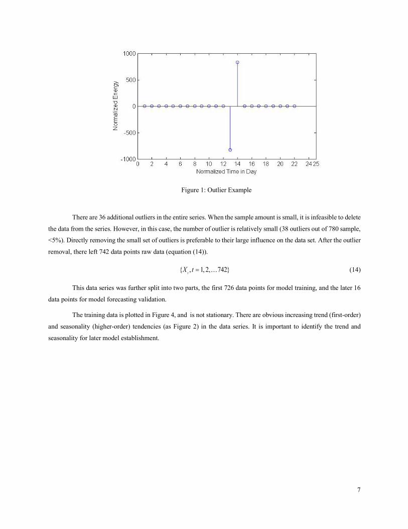
than the normal electricity consumption, so authors were confident in their exclusion from the analysis. Figure 1 is
the plot of subset of the data series with outliers. The x-axis represents the normalized time ( ) from 1 to 22, extending
daily from January 22nd 2014 to February 12th 2014. The y-axis represents the electrical energy, which has been
normalized to protect the information of the studied plant. It is obvious that there are two outliers at and .
( ), ( ), and ( , )MA q AR p ARMA p q( , , )ARMAX p d q
1 1 1
p qr
t i t i k t k t j t ji k j
X X U Z Zf b q- - -
= = =
= + + +å å å
2{ } ~ (0, )tZ WN s sf sq sb tU
4
1
( / ) ii
Electricity kWh Day Feeder=
=å
t
13t = 14t =
7
Figure 1: Outlier Example
There are 36 additional outliers in the entire series. When the sample amount is small, it is infeasible to delete
the data from the series. However, in this case, the number of outlier is relatively small (38 outliers out of 780 sample,
<5%). Directly removing the small set of outliers is preferable to their large influence on the data set. After the outlier
removal, there left 742 data points raw data (equation (14)).
(14)
This data series was further split into two parts, the first 726 data points for model training, and the later 16
data points for model forecasting validation.
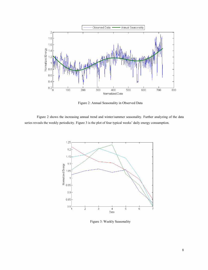
The training data is plotted in Figure 4, and is not stationary. There are obvious increasing trend (first-order)
and seasonality (higher-order) tendencies (as Figure 2) in the data series. It is important to identify the trend and
seasonality for later model establishment.
{ , 1, 2, 742}tX t = !
8
Figure 2: Annual Seasonality in Observed Data
Figure 2 shows the increasing annual trend and winter/summer seasonality. Further analyzing of the data
series reveals the weekly periodicity. Figure 3 is the plot of four typical weeks’ daily energy consumption.
Figure 3: Weekly Seasonality

9
Figure 3 x-axis represent the days 1 as Monday, 2 as Tuesday, and so on. The y-axis represents the normalized
energy consumption. The figure shows a relatively stable energy consumption during the weekdays, and lower energy
consumption on Saturdays and Sundays, as expected for the given production schedule.
The amount of available historical data (training data) will affect the model in two main ways. 1) Training
computational time. More training data will require more computation time to estimate the model parameters. 2) Trend
and seasonality. The larger the data set is, the better for trend and seasonality analysis. Take the example from our
studied case. Figure 4 shows more than two years of data. From this figure, we can clearly visualize the increasing
trend and annual seasonality in the data (see fitting increasing trend and annual seasonality in Figure 2). If we zoom
into weeks of data, it is also obvious to see the 7 days (weekly) seasonality (as Figure 3).
Figure 4: Historical Data Plot
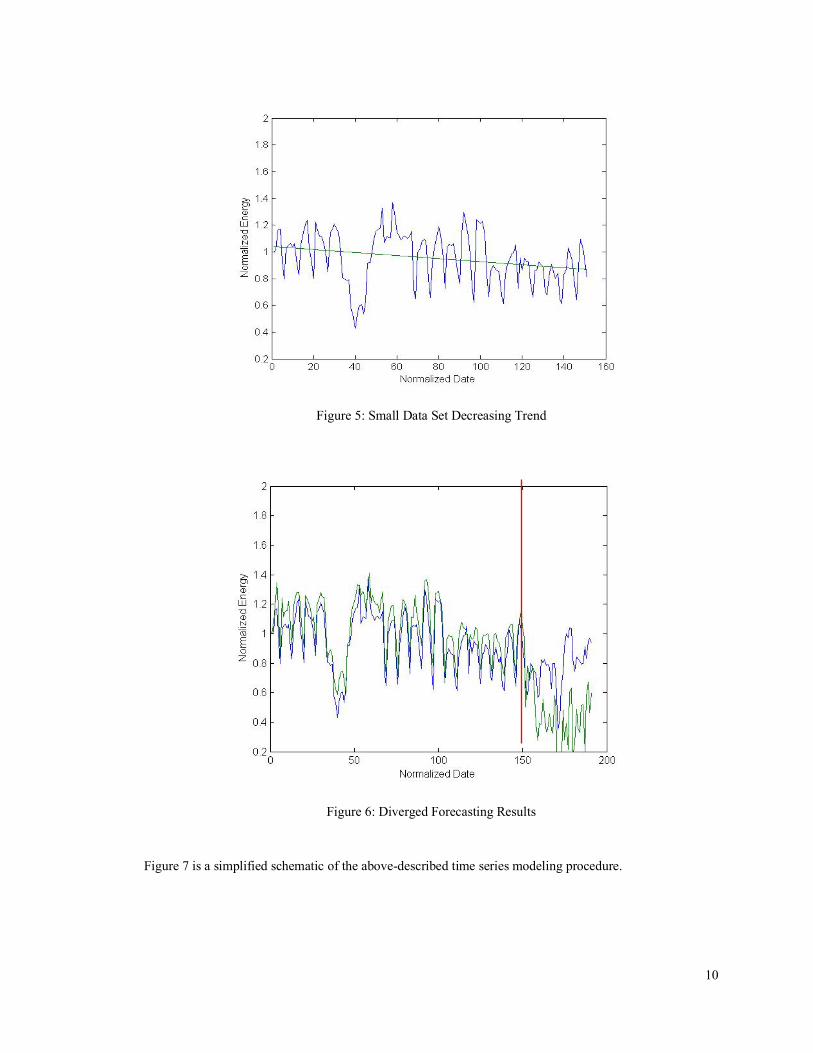
However, if the training data set is limited to a smaller data set, these features may not be so readily observed.
If we select only part of the data (e.g., smaller data set from t=1 to t=150, in this period of time, the training data set
shows a linear decreasing trend. Meanwhile, since the data only includes 150 days, it is impossible to get the annual
seasonality from it. Thus, when training, the model will be fitted with a simple decreasing linear trend (as Figure 5).
The fitted model may also behave well in forecasting the next few days’ results. However, if the fitted model is used
in the long run (selected model class with trained parameters), the results will diverge from the observed data (as
Figure 6).
10
Figure 5: Small Data Set Decreasing Trend
Figure 6: Diverged Forecasting Results
Figure 7 is a simplified schematic of the above-described time series modeling procedure.

11
Figure 7: Time Series Modeling Procedure
These two considerations of computation time and data length for periodicity identification can be solved in
the future with the help of big data analytics. With a big data system, it is expected to have a more efficient data
fetching and computational time. Updating the stored model parameters frequently by training the model with larger
data sets and more recent data inputs (i.e., frequently repeat the training procedures in Figure 7) will continue to make
forecasting results more accurate.
4.2 Model
By establishing a time series model, we can reveal the energy demand variation phenomenon in the
manufacturing plant; therefore, we can better understand the energy usage and plan for the next steps’ energy operation
and control strategy. Unlike the national electricity consumption example reviewed in the previous section, a local
manufacturing system is believed to have more predictable periodic factors based on working conditions. For example,
the energy used for the automotive assembly plant is shown to be related to the weather condition. Adding the
exogenous input of weather conditions into the time series model makes the forecasting result more robust and
interpretable. On the other hand, the known variables such as national holidays and vehicle production plan (i.e.,
number of vehicles being produced) can also be taken into the model for a better understanding the phenomenon in
the time series. More information of the key influential variables of automotive manufacturing plant was discussed in
paper [12].
Stationary Data Series Preparation
The observed training data are plotted in Figure 2 and are shown to be non-stationary. Before fitting the
model, the data need to be transformed into a stationary series. Autocorrelation function (ACF) and partial
autocorrelation function (PACF) are two functions that help identify the autocorrelation at different time lags (given
as equations (2) and (3)).

12
Figure 8: Training Data ACF
Figure 9: Training Data PACF
Figure 8 and Figure 9 are the ACF and PACF plot of training data respectively. Figure 8 shows a slow
degradation trend in the ACF value, with a first order trend effect, and strong correlation at time lag 7 and its harmonics.
This verifies the previously-described observations on the data trend and seasonality. Figure 9 also supports lag 7
seasonality.
In order to achieve a stationary time series, the trend and seasonality need to be removed from the original
data series; for this step a number of different techniques can be applied. Here, we assume the data series can be

13
represented as the additive form of the stationary series with trend and seasonality. Thus the new stationary series ,
can be written as Equation (4). One of the typical methods used to obtain the trend and seasonality is through
regression modeling and least squares estimation.
The original data series trend and seasonality can be represented in terms of regression fitting. By subtracting
the best fit given through least square estimation, a new data series without trend and seasonality can be achieved.
There are other approaches to detect and remove the trend and seasonality. Differencing is another
straightforward method in de-trending and de-seasonality, given as equations (5) – (8). To remove the trend and
seasonality, the difference as equation (15) can be applied to the training data series.
(15)
In Equation (15), the first order difference is to get rid of the increasing trend, the seventh order difference is
to remove the weekly seasonality, while the 365th order difference is to remove the annual seasonality.
No matter what de-trending and de-seasonality methods were use, a new stationary data series plot should
not show obvious trend and seasonality. After processing, the new data series is plotted as Figure 10, where has no
apparent trend and seasonality. Further examination of the expectation and covariance values (as Figure 11 and Figure
12), the new data series is qualified as weakly stationary (as defined in [13]).
Figure 10: New Data Series
tY
365 7 1
365 7(1 )(1 )(1 )
t t
t
Y X
B B B X
= Ñ Ñ Ñ
= - - -
tY

14
Figure 11: New Data Series Expectation Values
Figure 12: New Data Series Covariance Values
ACF and PACF can be applied to further examine the stationary data set. The new data series ACF and PACF
plots are in Figure 13 and Figure 14 respectively. The fast decreasing rate of ACF and PACF suggest there is no
obvious trend, but a relatively strong correlation at the time lag 7 suggests a possible MA(7) or AR(7) model.
tY
tY

15
Figure 13: ACF of
Figure 14: PACF of
Once the model is selected and the parameters estimated, the unit circle method (as equation (1)) can also be
used to help identify stationarity.
tY
tY

16
Model Selection
After the models are fitted, different criteria can be used to evaluate them. The Mean Square Error (MSE)
can be used to measure the accuracy. Beyond accuracy analysis, the problem of overfitting can be avoided by the
Akaike information criterion (AIC), Akaike information corrected criterion (AICC), and Bayesian information
criterion (BIC). AIC, AICC, and BIC, as well as the MSE can be calculated as:
(16)
(17)
(18)
(19)
From Equation (16) to (19), is the likelihood of models, are the parameters for auto-
regressive and moving average models respectively, are the orders of auto-regressive and moving average
models respectively, denotes the number of training data, is the training data, and is the estimated data.
All these four criteria can be used to aid in the model selection. The lower values of these criteria, the better
accuracy, and less likely the problem of overfitting. However, the AIC has a tendency to overestimate the order
[13]. The AICC and BIC has a greater penalty for large-order models, thus these two are more commonly used for
model selection; AICC is used in this work.
Both AICC is used as indicators to avoid the problem of overfitting. Table 1 provides the AICC indicators,
as well as the MSE of training data and MSE of the next 16 days’ forecasting. From this table, we can see the ARMA(7,
7) model has the smallest AICC, training MSE, and forecasting MSE, so it can be selected as a stationary
representation of the series.
Table 1: ARMA Model Test Results AICC Training MSE Forecasting MSE
AR(1) 683 1.75 0.88
( , )2 ln , , 2( 1)p q
p q
SAIC L p q
n
f qf q= - + + +æ öç ÷è ø
( , ) 2 ( 1)2 ln , ,
( 2)p q
p q
S n p qAICC L
n n p q
f qf q
+ += - +
- - -
æ öç ÷è ø
22
2
1( ) ln (1 ln 2 ) ( ) ln
n
tt
X nn
BIC n p q n p qn p q p q
ss
p =
-= - - + + + +
- - +
é ùê úé ùê úê úë û ê úë û
å !
! 2
1
1( )
n
i ii
MSE X Xn =
= -å
( )L × and i jf q
and p q
n tX ˆtX
p

17
AR(7) 651 7.32 2.09 MA(7) 581 1.71 0.26
ARMA(7,7) 412 0.97 0.16
Figure 15: ARMA Model Comparison
Figure 15 compares the forecasting results from four ARMA models. As the figure shows, ARMA(7, 7)
model is better in flowing the data.
Exogenous Inputs
As stated before, the automotive manufacturing plant has many features that can be taken as exogenous inputs
into the time series model to make it more robust and interpretable. From the previous lower-level analysis, the
sensible variables are from three main aspects – weather, productivity, and working days. These three aspects were
further developed into the following vector representation:
, (20)
where is the exogenous inputs/sensible variables matrix, and
, (21)
tY
[ ]Weather Productivity Working Days=u
u
[ ]avg Max Min Max MinWeather T T T CDD HDD rH rH= !

18
where represents the temperature, represents the relative humidity, the cooling degree days,
heating degree days; subscript denotes the average value in one day, denotes the maximum value in one
day, and denotes the minimum value in one day.
(22)
where represents the number of vehicles produced in one day; subscript
denotes the vehicle model from department .
, (23)
where represents the day in a week, represents the non-working/working days condition, and
represents the maintenance condition. Other variables can also be included in the matrixes. Then the exogenous inputs
in (20) can be written as (24).
(24)
where represents the exogenous input at time .
In this studied case, four independent variables ( ) were selected – CDD ( ), working/nonworking
days ( ), total number of Vehicle Type I made in one day ( ), and total number of Vehicle Type II made in
one day ( ) (as Equation (25)).
T rH CDD HDD
avg Max
Min
1,1 2,1 3,1 ,Productivity [ ]m nV V V V= !
V (i, j)={(1, 1) (2, 1) (3, 1) ... (m, n)}
i j
Working Days [ ]D NW MT= !
D thi NW MT
1,1 1,2 1,
2,1 2,2 2,
,1 ,2 ,
j
j
t t t j
u u u
u u u
u u u
=
é ùê úê úê úê úë û
!
!
" " # "
!
u
,i juthj t
u iCDD
iNWD iVA
iVB

19
(25)
ARMAX with different orders were tested (as Equation (12)). The model with the given exogenous inputs
shows improvements in AIC and MSE (as Table 2). The fitted models have an absolute value of auto-regressive
parameters smaller than 1, which means the unit roots tested stationary. Among all the ARMAX model, ARMAX(7,
7, 5) performs best with AIC of 21.91 and forecasting MSE of 0.0154.
Table 2: ARMAX Model Test Results AIC Training MSE Forecasting MSE
ARMAX(7,7,5) 21.91 0.0068 0.0154 ARMAX(0,7,5) 21.99 0.0072 0.0327 ARMAX(7,0,5) 21.92 0.0069 0.0195
4.3 Model Comparison
The models with exogenous inputs and the best fit of ARMA model are shown here for comparison.
Figure 16: Model Forecasting Results Comparison
1 1 1 1
2 2 2 2
t t t t
CDD NWD VA VB
CDD NWD VA VB
CDD NWD VA VB
=
é ùê úê úê úê úë û
! ! ! !u

20
Figure 16 shows how the time series model performs better with exogenous inputs, especially in days with a
sudden change with assignable cause. ARMAX is much better at forecasting when . This is because, during this
period of time, the plant begins to produce after a long shutdown. The ARMAX model follows the sudden energy
increase right after the shutdown ( ), while it takes ARMA(7, 7) model a longer time (after ) to follow the
increase.
It is obvious that the traditional time series models cannot quickly follow the sudden energy consumption
change, nor are they more accurate than the ARMAX model. With the exogenous inputs from the ARMAX model the
accuracy is much improved (in terms of MSE) and more robust to the predicable and scheduled changes.
Residual Randomness
The residuals from the ARMAX(7, 7, 5) were also tested.
Figure 17: Scatterplot of Residuals
Figure 17 is the scatter plot of residuals. This figure does not show obvious mean and variation value change
over the orders, i.e., the residual values are independent on orders.
Figure 18 shows a histogram distribution of the residuals. It indicates randomness and distribution about 0,
so we can assume no unmodeled effects remain.
5t ³
5t = 11t =

21
Figure 18: Residual Normally Distributed
Further analyses of ACF and PACF of the residuals (as Figure 19 and Figure 20) indicates no correlations
among the residuals, i.e., the residuals are random.
Figure 19: ACF of Residuals
0.450.300.150.00-0.15-0.30-0.45
250
200
150
100
50
0
Mean 0.002810StDev 0.08246N 726
Residual
Freq
uenc
y
Histogram of ResidualNormal

22
Figure 20: PACF of Residuals
5 CONCLUSION AND FUTURE WORK
In this research work, time series models from the mathematical domain were introduced to forecast the
energy demand in the manufacturing domain. Influential variables for an automotive manufacturing plant were
introduced into time series models as exogenous inputs to increase the model accuracy and robustness. The ARMAX
models with exogenous inputs show a better accuracy in MSE and are more robust to the sudden deviations. From the
results of the time series models developed in this paper, it is observable that the energy demand of this plant has kept
increasing and is highly seasonal (annual and weekly seasonality in the energy consumption showed in the studied
case). The energy demand forecasting results are essential to intelligently schedule the production, manage the
working conditions, and stabilize energy supply. It can also assist in the understanding on how the manufacturing
plants affect the local energy distribution.
Regarding future work, time series promises to be further applied into real-time forecasting. The real time
outputs can be used as constraints for on-site energy conversion and transmission optimization. It would also be
interesting to augment the proposed modeling approach to include other types of resources, such as natural gas, steam,
water, and even the flow of parts materials.
ACKNOWLEDGMENT
The authors would like to thank BMW Manufacturing Co. for their project sponsorship and access to the
manufacturing facility.
References

23
[1] L. Feng, L. Mears, C. Beaufort and J. Schulte. Energy, economy, and environment analysis and optimization on
manufacturing plant energy supply system. Energy Conversion and Management 117pp. 454-465. 2016. . DOI:
http://dx.doi.org/10.1016/j.enconman.2016.03.031.
[2] T. Samak, C. Morin and D. Bailey. Energy consumption models and predictions for large-scale systems. Presented
at Parallel and Distributed Processing Symposium Workshops & PhD Forum (IPDPSW), 2013 IEEE 27th
International. 2013, . DOI: 10.1109/IPDPSW.2013.228.
[3] S. J. Taylor, Modelling Financial Time Series (Second Edition). World Scientific Publishing, 2007.
[4] H. Kömm and U. Küsters. Forecasting zero-inflated price changes with a markov switching mixture model for
autoregressive and heteroscedastic time series. Int. J. Forecast. 31(3), pp. 598-608. 2015. . DOI:
http://dx.doi.org/10.1016/j.ijforecast.2014.10.008.
[5] S. Saab, E. Badr and G. Nasr. Univariate modeling and forecasting of energy consumption: The case of electricity
in lebanon. Energy 26(1), pp. 1-14. 2001. . DOI: http://dx.doi.org/10.1016/S0360-5442(00)00049-9.
[6] R. E. Abdel-Aal and A. Z. Al-Garni. Forecasting monthly electric energy consumption in eastern saudi arabia
using univariate time-series analysis. Energy 22(11), pp. 1059-1069. 1997. . DOI: http://dx.doi.org/10.1016/S0360-
5442(97)00032-7.
[7] P. G. Gould, A. B. Koehler, J. K. Ord, R. D. Snyder, R. J. Hyndman and F. Vahid-Araghi. Forecasting time series
with multiple seasonal patterns. Eur. J. Oper. Res. 191(1), pp. 207-222. 2008. . DOI:
http://dx.doi.org/10.1016/j.ejor.2007.08.024.
[8] S. S. Pappas, L. Ekonomou, D. C. Karamousantas, G. E. Chatzarakis, S. K. Katsikas and P. Liatsis. Electricity
demand loads modeling using AutoRegressive moving average (ARMA) models. Energy 33(9), pp. 1353-1360. 2008. .
DOI: http://dx.doi.org/10.1016/j.energy.2008.05.008.
[9] C. E. Asbury. Weather load model for electric demand and energy forecasting. Power Apparatus and Systems,
IEEE Transactions On 94(4), pp. 1111-1116. 1975. . DOI: 10.1109/T-PAS.1975.31945.
[10] Y. Li, Y. Su and L. Shu. An ARMAX model for forecasting the power output of a grid connected photovoltaic
system. Renewable Energy 66pp. 78-89. 2014. . DOI: http://dx.doi.org/10.1016/j.renene.2013.11.067.
[11] J. R. Cancelo, A. Espasa and R. Grafe. Forecasting the electricity load from one day to one week ahead for the
spanish system operator. Int. J. Forecast. 24(4), pp. 588-602. 2008. . DOI:
http://dx.doi.org/10.1016/j.ijforecast.2008.07.005.
[12] L. Feng, L. Mears and J. and Schulte, "Key variable analysis and identification on energy consumption of
automotive manufacturing plant," in 4Th Annual IEEE Conference on Technologies for Sustainability, 2016, .
[13] P. J. Brockwell and R. A. Davis, Introduction to Time Series and Forecasting. New York: Springer-Verlag, 2002.