San Jose State University San Jose State University

SJSU ScholarWorks SJSU ScholarWorks

Master's Theses Master's Theses and Graduate Research

Spring 2011

Energy and Exergy Analysis of Data Center Economizer Systems Energy and Exergy Analysis of Data Center Economizer Systems

Michael Elery Meakins San Jose State University

Follow this and additional works at: https://scholarworks.sjsu.edu/etd_theses

Recommended Citation Recommended Citation Meakins, Michael Elery, "Energy and Exergy Analysis of Data Center Economizer Systems" (2011). Master's Theses. 3944. DOI: https://doi.org/10.31979/etd.bf7d-khxd https://scholarworks.sjsu.edu/etd_theses/3944

This Thesis is brought to you for free and open access by the Master's Theses and Graduate Research at SJSU ScholarWorks. It has been accepted for inclusion in Master's Theses by an authorized administrator of SJSU ScholarWorks. For more information, please contact scholarworks@sjsu.edu.

ENERGY AND EXERGY ANALYSIS OF

DATA CENTER ECONOMIZER SYSTEMS

A Thesis

Presented to

The Faculty of the Department of Mechanical and Aerospace Engineering

San José State University

In Partial Fulfillment

of the Requirements for the Degree

Master of Science

By

Michael E. Meakins

May 2011

© 2011

Michael E. Meakins

ALL RIGHTS RESERVED

The Designated Thesis Committee Approves the Thesis Titled

ENERGY AND EXERGY ANALYSIS OF DATA CENTER ECONOMIZER SYSTEMS

by

Michael E. Meakins

APPROVED FOR THE DEPARTMENT OF MECHANICAL AND AEROSPACE ENGINEERING

SAN JOSÉ STATE UNIVERSITY

May 2011

Dr. Nicole Okamoto Department of Mechanical and Aerospace Engineering

Dr. Jinny Rhee Department of Mechanical and Aerospace Engineering

Mr. Cullen Bash Hewlett Packard Labs

ABSTRACT

ENERGY AND EXERGY ANALYSIS OF DATA CENTER ECONOMIZER SYSTEMS

By Michael E. Meakins

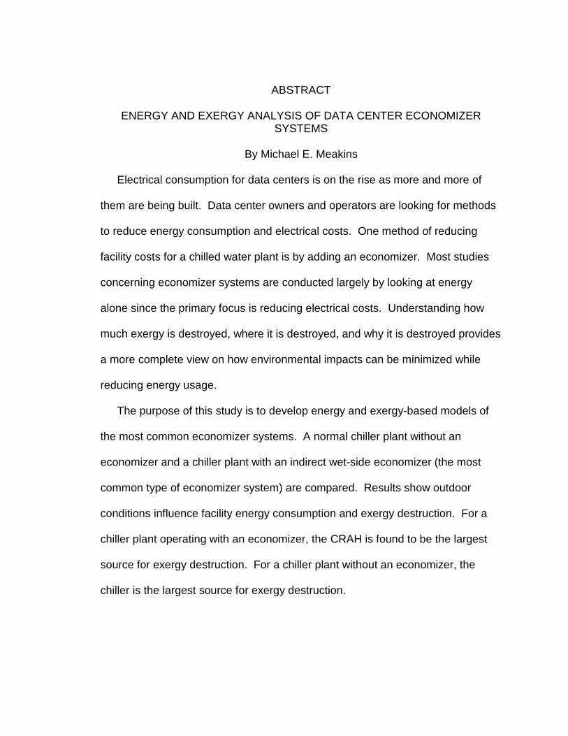
Electrical consumption for data centers is on the rise as more and more of

them are being built. Data center owners and operators are looking for methods

to reduce energy consumption and electrical costs. One method of reducing

facility costs for a chilled water plant is by adding an economizer. Most studies

concerning economizer systems are conducted largely by looking at energy

alone since the primary focus is reducing electrical costs. Understanding how

much exergy is destroyed, where it is destroyed, and why it is destroyed provides

a more complete view on how environmental impacts can be minimized while

reducing energy usage.

The purpose of this study is to develop energy and exergy-based models of

the most common economizer systems. A normal chiller plant without an

economizer and a chiller plant with an indirect wet-side economizer (the most

common type of economizer system) are compared. Results show outdoor

conditions influence facility energy consumption and exergy destruction. For a

chiller plant operating with an economizer, the CRAH is found to be the largest

source for exergy destruction. For a chiller plant without an economizer, the

chiller is the largest source for exergy destruction.

v

ACKNOWLEDGEMENTS

It is my pleasure to thank the many people who made this thesis possible.

I would like to express my sincere thanks to my committee chair, Dr. Nicole

Okamoto, for her continuous guidance throughout the development and

completion of the thesis. My sincere thanks to my committee members, Mr.

Cullen Bash and Dr. Jinny Rhee for their advice and suggestions during the

development throughout the course of the thesis. Lastly, and most importantly, I

wish to thank my wife and sons for their patience and support all the way through

my thesis. Without their devoted support, this thesis would have not been

possible.

vi

CONTENTS

NOMENCLATURE ............................................................................................ VIII

LIST OF FIGURES .............................................................................................. XI

LIST OF TABLES .............................................................................................. XIII

CHAPTER 1 INTRODUCTION ......................................................................... 1

1.1 Motivation ........................................................................................ 1

1.2 Literature Review ............................................................................ 2

CHAPTER 2 METHODOLOGY ...................................................................... 12

2.1 Simulation Overview ..................................................................... 12

2.2 Cooling Tower Component ........................................................... 13

2.3 Chiller Component ........................................................................ 17

2.4 Plate and Frame Heat Exchanger ................................................. 23

2.5 Makeup Air Handler ...................................................................... 26

2.6 Computer Room Air Handler ......................................................... 27

2.7 General Exergy Theory - Air Side ................................................. 28

2.8 General Exergy Theory – Open Systems ...................................... 30

2.9 Simulation Modeling ...................................................................... 31

2.10 Data Center Heat Load ................................................................. 32

2.11 Data Center Facility Modeling Inputs ............................................ 34

CHAPTER 3 RESULTS .................................................................................. 37

3.1 Make-up Air Handler ..................................................................... 37

3.2 Cooling Tower ............................................................................... 41

vii

3.3 Economization Hours .................................................................... 43

3.4 Energy Consumption ..................................................................... 43

3.5 Energy Efficiency .......................................................................... 46

3.6 Exergy Destruction ........................................................................ 51

CHAPTER 4 CONCLUSION ........................................................................... 58

4.1 Future Work .................................................................................. 59

REFERENCES ................................................................................................... 60

APPENDICES .................................................................................................... 68

A.1 Indirect Wet-side Economizer (IWE) ............................................. 68

A.2 EES CODE ................................................................................... 69

viii

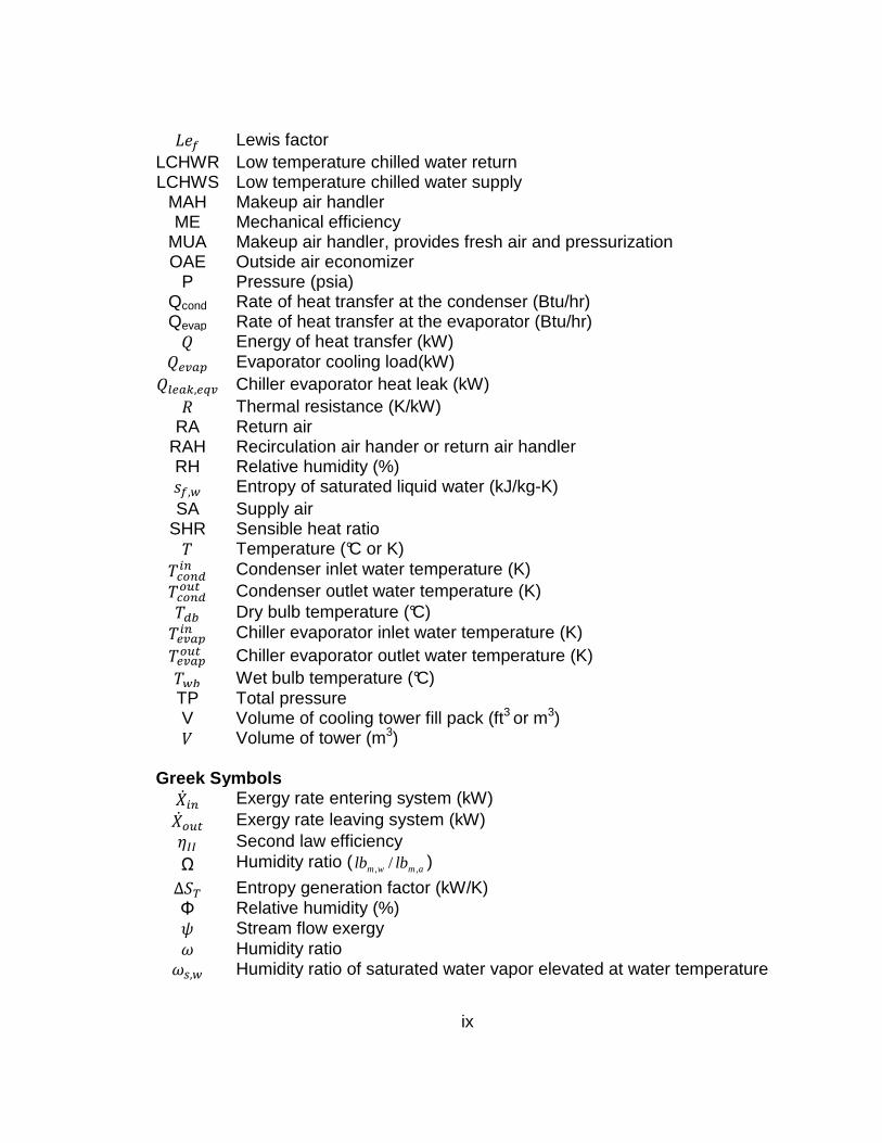
NOMENCLATURE

A Cross sectional area of fill pack (m2) AHU Air handler unit BHP Brake horsepower CD Condensate drain

CFM Cubic feet per minute (ft3/min) CHWR Chilled water return CHWS Chilled water supply COP Coefficient of performance (W/W)

CRAC Computer room air conditioner CRAH Computer room air handler

CT Cooling tower CWR Condenser water return CWS Condenser water supply CV Control valve Cp Specific heat (btu/lbm-R) or (kJ/kg-K) , Specific heat of dry air at constant pressure (kJ/kg-K) , Specific heat of water vapor at constant pressure (kJ/kg-K) , Specific heat of water at constant pressure (kJ/kg-K) Differential enthalpy (kJ/kg) Differential height of cooling tower fill (m)

DWE Direct wet-side economizer ESP External static pressure EWT Entering water temperature Exergy FHP Fan horsepower Dry air mass flow rate (kg/s)

H Height of cooling tower fill pack (m) Enthalpy (kJ/kg) , Enthalpy of water vapor (kJ/kg) , Enthalpy of liquid water (kJ/kg) HUW Humidification water HWR Hot water return HWS Hot water supply HVAC Heating ventilation air-conditioning

IW Industrial water IWE Indirect wet-side economizer Tower characteristic (kg/m3-s)

kW/ton Power consumption per ton of useful refrigeration (kW/Ton) LWT Leaving water temperature Water mass flow rate (kg/s)

ix

Lewis factor LCHWR Low temperature chilled water return LCHWS Low temperature chilled water supply

MAH Makeup air handler ME Mechanical efficiency

MUA Makeup air handler, provides fresh air and pressurization OAE Outside air economizer

P Pressure (psia) Qcond Rate of heat transfer at the condenser (Btu/hr) Qevap Rate of heat transfer at the evaporator (Btu/hr) Energy of heat transfer (kW) Evaporator cooling load(kW) , Chiller evaporator heat leak (kW) Thermal resistance (K/kW) RA Return air

RAH Recirculation air hander or return air handler RH Relative humidity (%) , Entropy of saturated liquid water (kJ/kg-K) SA Supply air

SHR Sensible heat ratio Temperature (°C or K) Condenser inlet water temperature (K) ! Condenser outlet water temperature (K) " Dry bulb temperature (°C) Chiller evaporator inlet water temperature (K) ! Chiller evaporator outlet water temperature (K) " Wet bulb temperature (°C) TP Total pressure V Volume of cooling tower fill pack (ft3 or m3) # Volume of tower (m3)

Greek Symbols $% Exergy rate entering system (kW) $% ! Exergy rate leaving system (kW) &'' Second law efficiency

Ω Humidity ratio ( amwm lblb ,, / )

Δ)* Entropy generation factor (kW/K) Φ Relative humidity (%) + Stream flow exergy , Humidity ratio ,-, Humidity ratio of saturated water vapor elevated at water temperature

x

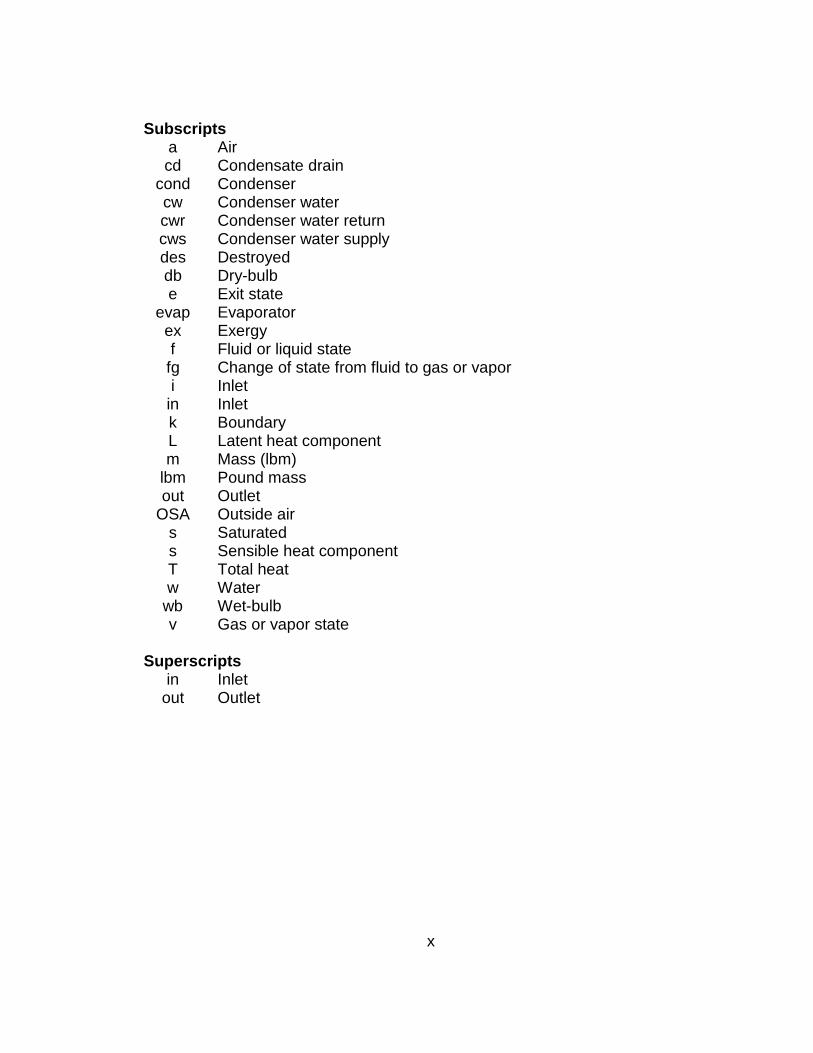
Subscripts a Air cd Condensate drain

cond Condenser cw Condenser water cwr Condenser water return cws Condenser water supply des Destroyed db Dry-bulb e Exit state

evap Evaporator ex Exergy f Fluid or liquid state fg Change of state from fluid to gas or vapor i Inlet

in Inlet k Boundary L Latent heat component m Mass (lbm)

lbm Pound mass out Outlet

OSA Outside air s Saturated s Sensible heat component T Total heat w Water

wb Wet-bulb v Gas or vapor state

Superscripts

in Inlet out Outlet

xi

LIST OF FIGURES

Figure 1.1: Water cooled chiller plant ................................................................... 4

Figure 1.2: Integrated indirect wet-side economizer ............................................. 6

Figure 1.3: Cooling system examples for a generic chiller plant and

different types of economizers ....................................................................... 8

Figure 2.1: Differential element of mass and energy balance for a counter

flow wet cooling tower ................................................................................. 14

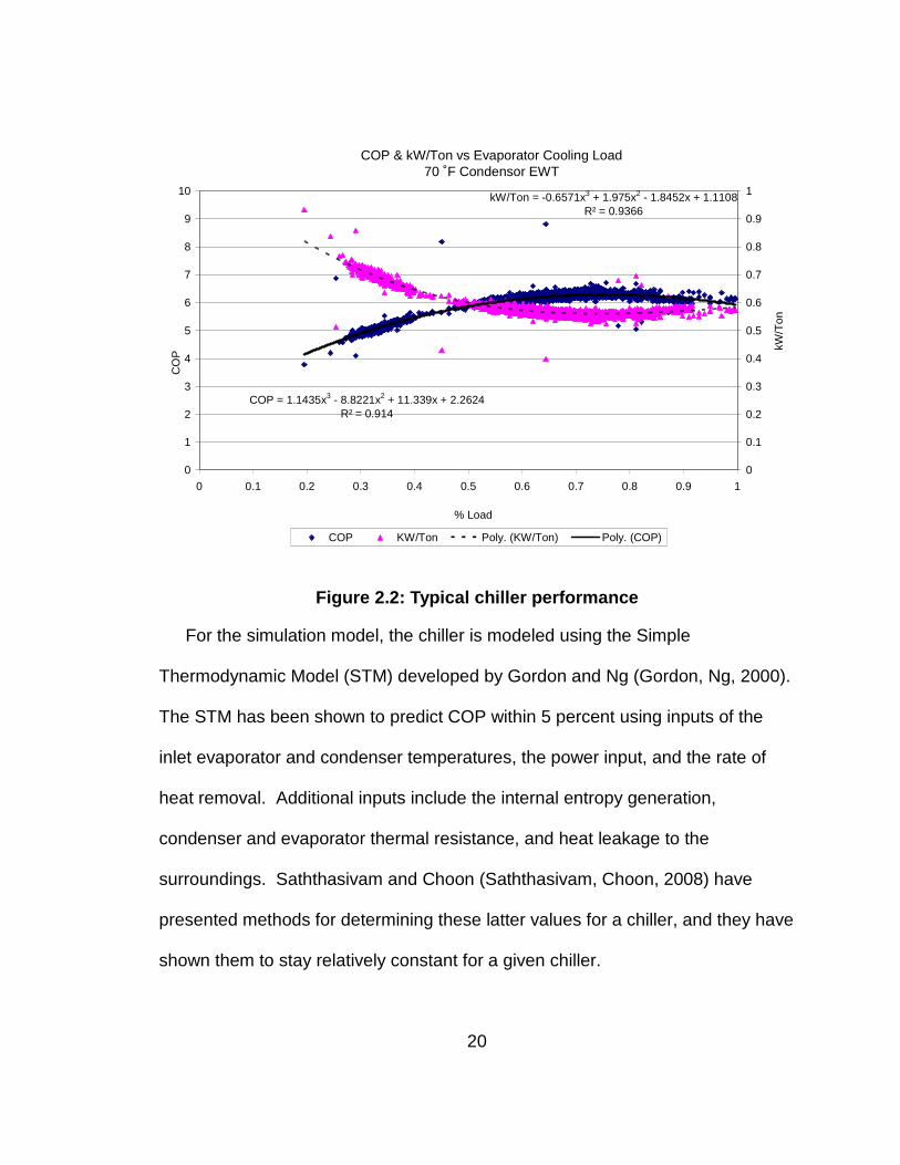
Figure 2.2: Typical chiller performance ............................................................... 20

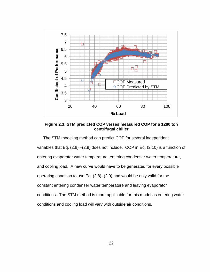
Figure 2.3: STM predicted COP verses measured COP for a 1280 ton

centrifugal chiller.......................................................................................... 22

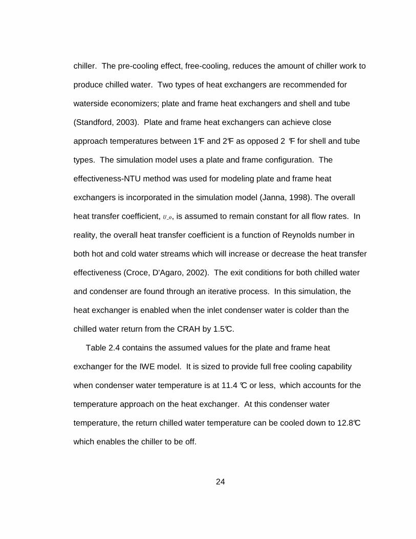
Figure 2.4: Plate and frame heat exchanger performance ................................. 26

Figure 2.5: Makeup air handler schematic .......................................................... 27

Figure 2.6: Computer room air handler (CRAH) model ...................................... 28

Figure 3.1: Makeup air absolute energy usage for different dry bulb and

relative humidity conditions ......................................................................... 38

Figure 3.2: Makeup air handler absolute total energy usage for a 24-hour

period with varying wet bulb conditions ....................................................... 39

Figure 3.3: San Francisco weather bin data and projected MUA energy

usage ........................................................................................................... 40

Figure 3.4: MUA energy transfer on warmest day in San Francisco ................... 41

Figure 3.5: Evaporative cooling tower energy usage on warmest day for

San Francisco ............................................................................................. 42

xii

Figure 3.6: Chiller plant with an integrated indirect wet-side economizer

energy efficiency performance (kW/ton) versus outside air dry-bulb

temperature ................................................................................................. 47

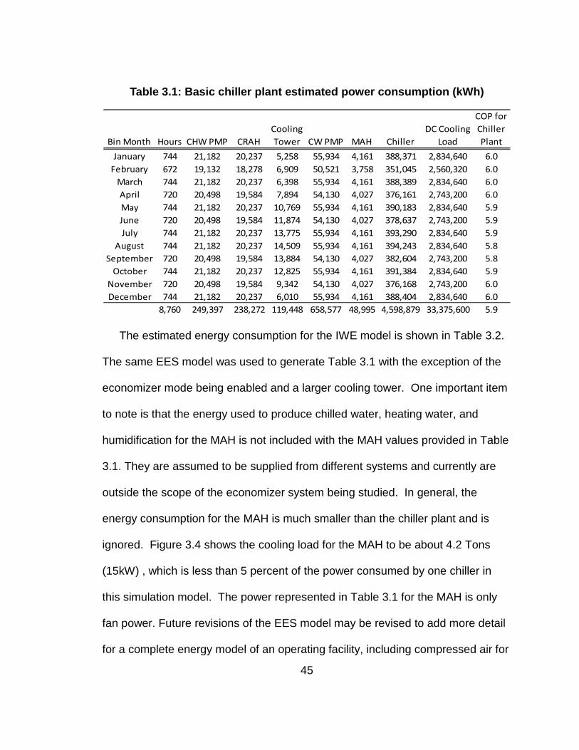
Figure 3.7: Chiller plant with an integrated indirect wet-side economizer

energy efficiency performance (kW/ton) versus outside air wet-bulb

temperature ................................................................................................. 49

Figure 3.8: Total exergy destroyed versus outdoor dry-bulb temperature

for chilled water plant with IWE ................................................................... 56

Figure 3.9: 2nd Law efficiency plot for wet-bulb temperature for chilled

water plant with IWE .................................................................................... 57

xiii

LIST OF TABLES

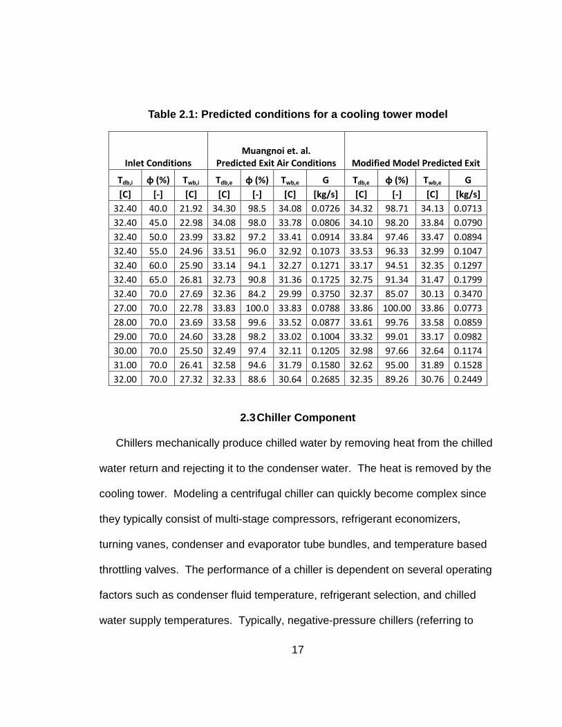
Table 2.1: Predicted conditions for a cooling tower model ................................. 17

Table 2.2: ARI standard rating conditions for a water-cooled chiller ................... 18

Table 2.3: Simple thermodynamic model parameters ........................................ 23

Table 2.4: Plate and frame model parameters.................................................... 25

Table 2.5: Example of data center heat load calculations .................................. 33

Table 2.6: Data center facility modeling inputs ................................................... 35

Table 3.1: Basic chiller plant estimated power consumption (kWh) .................... 45

Table 3.2: Estimated power consumption with an integrated wet-side

economizer (kWh) ....................................................................................... 46

Table 3.3: Exergy destroyed without an economizer (kWh) ............................... 52

Table 3.4: Exergy destroyed with an economizer (kWh) .................................... 54

1

CHAPTER 1 INTRODUCTION

1.1 Motivation

According to an Environmental Protection Agency (EPA) report on energy

efficiency in data centers, their electrical power demand could double from 2007

to 2011 in the United States (United States Environmental Protection Agency,

2007). The report indicates that electrical demand for data centers in 2006 was

1.5 percent of the total of all electrical demand in the US and will increase to 2.5

percent. The EPA report emphasizes that there are opportunities for data

centers to improve their efficiencies, both on the facility and server sides of data

center infrastructure. The average data center facility will use about 0.83 Watts

of power for facility infrastructure, including cooling, for every 1 Watt of critical

information technology (IT) power demand (Greenberg, 2007; United States

Environmental Protection Agency, 2007). Chiller systems are typically the

largest consumer of electrical demand, second only to critical IT demands

(Koomey, 2004). The use of economizer systems is one method to reduce

energy consumption for data centers by significantly lowering cooling cost.

The purpose of this study has been to develop energy and exergy-based

models of one of the most common economizer systems. The models

incorporate weather bin data, which will allow users to determine the energy and

cost savings for the most common of economizer system for their locale. The

models can also be used to determine which components result in the most

exergy losses, allowing researchers to better focus their efforts to improve these

2

systems. They can also be used to analyze the electrical energy and exergy

savings under a variety of conditions such as raising the data center supply or

return air temperatures or changing the cooling load. In this paper, a normal

chiller plant without an economizer and a chiller plant with an indirect wet-side

economizer (the most common type of economizer system) are compared.

1.2 Literature Review

The simulation of cooling system performance in the past was largely energy

based. Now studies are being published that perform exergy-based analysis to

determine maximum efficiency and evaluate the quality of energy conversions

(Harutunian, 2003; Liu, 1994; Paulus, 2000; Wang, 2005; Wu, 2004). An exergy

analysis (also called availability analysis) determines the maximum useful work

than can result when a system goes through a process between two specific

states or the minimum required for cooling between two states. Applying exergy

balances to a system allows for a direct comparison of the amount of work

potential supplied to the amount of that has been consumed (Kotas, 1995). A

measurement of exergy destruction allows one to determine the work potential

destroyed by each system or component due to irreversibility.

A significant amount of work has been published utilizing exergy analysis to

evaluate heating ventilation air-conditioning (HVAC) system performance for

general components and configurations. Reference texts have been published

on the exergy method (Bejan, 2006; Bejan, Tsatsaronis, Moran, 1996) and

evaluation of thermal plant efficiencies (Kotas, 1995). Moist air exergy balances

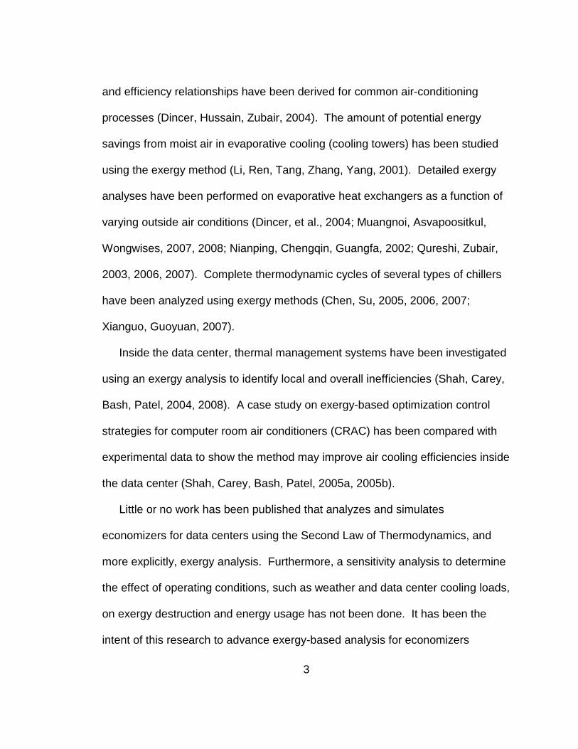
3

and efficiency relationships have been derived for common air-conditioning

processes (Dincer, Hussain, Zubair, 2004). The amount of potential energy

savings from moist air in evaporative cooling (cooling towers) has been studied

using the exergy method (Li, Ren, Tang, Zhang, Yang, 2001). Detailed exergy

analyses have been performed on evaporative heat exchangers as a function of

varying outside air conditions (Dincer, et al., 2004; Muangnoi, Asvapoositkul,

Wongwises, 2007, 2008; Nianping, Chengqin, Guangfa, 2002; Qureshi, Zubair,

2003, 2006, 2007). Complete thermodynamic cycles of several types of chillers

have been analyzed using exergy methods (Chen, Su, 2005, 2006, 2007;

Xianguo, Guoyuan, 2007).

Inside the data center, thermal management systems have been investigated

using an exergy analysis to identify local and overall inefficiencies (Shah, Carey,

Bash, Patel, 2004, 2008). A case study on exergy-based optimization control

strategies for computer room air conditioners (CRAC) has been compared with

experimental data to show the method may improve air cooling efficiencies inside

the data center (Shah, Carey, Bash, Patel, 2005a, 2005b).

Little or no work has been published that analyzes and simulates

economizers for data centers using the Second Law of Thermodynamics, and

more explicitly, exergy analysis. Furthermore, a sensitivity analysis to determine

the effect of operating conditions, such as weather and data center cooling loads,

on exergy destruction and energy usage has not been done. It has been the

intent of this research to advance exergy-based analysis for economizers

4

systems by developing specific mathematical models for data center HVAC

systems. Figure 1.1 is a simple facility diagram used for this study, it represents

a chiller plant without any economization features. Figure 1.2 is a simple facility

diagram of a chiller plant with an integrated wet-side economizer.

Figure 1.1: Water cooled chiller plant

For this type of integrated wet-side economizer in Figure 1.2, the heat

exchanger indirectly produces chilled water or pre-cool chilled water before

reaching the chiller. As servers produce heat in the data center, a return air

handler (RAH) removes the heat and then rejects the unwanted heat to the

5

chilled water system. The RAH performs many useful functions to maintain the

environmental conditions inside the data center, such as filtering air

contaminants, latent and sensible cooling, moving the air, and humidity controls.

The chilled water is moved by a chilled water pump through the heat exchanger,

water-cooled chiller and back to the RAH.

The condenser water loop has a pump that moves condenser water from the

cooling tower to the heat exchanger. If the condenser water returning from the

cooling tower is colder than the chilled water returning from the RAH, the heat

exchanger provides a means to transfer heat to the condenser water while

bypassing and therefore avoiding mixing the two water streams. Open cooling

tower water is generally considered dirty because it is exposed to outdoor

elements that may contain solids that cause fouling in RAH heat exchangers

coils and chiller bundle tubes. In general, open loop cooling tower water is not

allowed to mix with a closed loop chilled water system because of this fouling

and other operational issues. The heat that the heat exchanger removes

ultimately reduces the cooling load on the chiller.

The chiller utilizes a vapor refrigeration cycle to remove heat from the chilled

water and then transfers the heat to the condenser water loop. Pumps move the

condenser water to the cooling tower where it can then be rejected to the outside

air by means of evaporative cooling. The warm condenser water cools down and

then returns back to the heat exchanger and chiller. These systems operate

together to remove heat from the data center to the outside air. The wet-side

6

economizer feature, utilizing a heat exchanger to pre-cool warm chilled water

return, reduces the amount of cooling required from the chiller. The make-up air

handler (MAH) in Figure 1.2 provides fresh air to the data center. The MAH can

also be used to positively pressurize the data center relative to other areas in the

building. Dust and air infiltration is minimized. Since the MAH brings in outside

air, it has components to condition the outside air before it is allowed to mix with

inside air. These components provide filtration, heating, humidification control,

cooling, and moving the air.

Figure 1.2: Integrated indirect wet-side economizer

7

Economizers, or “free-cooling,” are mechanical systems that save energy by

reducing the amount of refrigeration compressor work required to provide cooling

when outside air conditions are favorable. The energy consumed for a waterside

economizers, only pumps and fan energy, is 15 to 20 percent of the energy

required from refrigeration cooling (Standford, 2003). The use of economizers to

save energy for various cooling applications is not new, and several case studies

have been published (Imperatore, 1975; Starr, 1984; Telecky, 1985; Tobias,

Schade, 1976; Zmeureanu, 1988). The use of economizers (free cooling) and

raising supply or return air temperatures are only two of many possible methods

of reducing the cooling costs for data centers (Garday, 2007; Kurkjian, Glass,

Routsen, 2007; Schmidt, Beaty, Dietrich, 2007; Sorell, 2007; Tschudi, Fok,

2007). These systems may use outside air, direct wet-side evaporative heat

exchangers, or indirect wet-side chilled water loops for cooling (Taras, 2005).

When it is more economical to bring in fresh supply air rather than to cool the hot

return air, the outside air economizer (OAE) uses partial to 100% outside air to

provide cooling. In both direct wet-side (DWE) and indirect wet-side economizer

(IWE) systems, a cooling tower can directly provide the production of chilled

water when the outdoor wet bulb temperature is below the desired chilled water

supply set point temperature. The DWE system circulates the cooling fluid

directly to the cooling tower and back to the air handler, which directly or partially

produces chilled water. The IWE system uses an intermediate heat exchanger

between the cooling tower, chiller, and air handler, which indirectly produces

8

chilled water. The IWE can pre-cool chilled water return prior to reaching the

chiller to save energy or operate in 100 percent free-cooling mode that bypasses

the chiller completely. Figure 1.3 illustrates the OAE, DWE, and IWE typical

system configurations (Taras, 2005).

Figure 1.3: Cooling system examples for a generic c hiller plant and different types of economizers

9

The use of these economizing systems is gaining traction worldwide because

case studies have shown them to be economical (Fisk, Seppänen, Faulkner,

Huang, 2005; Garday, 2007; Taras, 2005). Rising electrical rates, higher heat

load densities, increasing cooling requirements, and energy conscious rebate

programs are improving the payback on capital outlays required to install

potentially more complicated facility systems (United States Environmental

Protection Agency, 2007). Some local and state governments have adopted

energy codes that require the use of economizers (Department of Planning and

Development, 2006; Oregon Department of Energy, 2007).

The simulations of cooling systems’ performance have been largely energy

based, and now studies are being published that perform exergy-based analysis

to determine maximum efficiency and evaluate the quality of energy conversions.

Exergy is defined as “the maximum useful work than can be obtained as a

system undergoes a process between two specific states” (Cengel, Boles, 2006).

Availability analysis is another name commonly used to describe exergy analysis.

Applying exergy balances to a system allows for comparison of direct

measurement of the amount of work potential supplied to the amount of that has

been consumed (Kotas, 1995). Exergy analysis measures the amount of work

potential or the quality of different forms of energy relative to the environment. It

is also used for designing, improving, and optimizing thermal fluid system

designs.

10

A significant amount of work has been published utilizing exergy analysis to

evaluate heating ventilation air-conditioning (HVAC) system performance for

general components and configurations. Reference texts have been published

on the exergy method (Bejan, 2006; Bejan, et al., 1996) and evaluating thermal

plant efficiencies (Kotas, 1995). Moist air exergy balances and efficiency

relationships have been derived for common air-conditioning processes

(Kanoglu, Dincer, Rosen, 2007). Exergy analysis has been conducted on

evaporative heat exchangers, also known as cooling towers (Qureshi, 2004).

The amount of potential energy savings from moist air in evaporative cooling has

been studied using exergy method (Li, et al., 2001). Detailed chiller exergy

analyses have been performed on evaporative heat exchangers as a function of

varying outside air conditions (Muangnoi, et al., 2007; Naphon, 2005; Nianping,

et al., 2002; Qureshi, 2004; Qureshi, Zubair, 2007). Others have studied the

refrigeration cycle in detail for different types of configurations. The vapor

compression refrigeration plant cycle has been analyzed by trending compressor

speeds and selecting different types of refrigerants (Aprea, Rossi, Greco, Renno,

2003). Complete thermodynamic cycles of several types of chillers have been

analyzed using exergy methods (Chen, Su, 2005; Tsaros, 1987; Tschudi, Fok,

2007; Xianguo, Guoyuan, 2007). A modified coefficient of performance (COP)

has been developed to be exergy based (Hasabnis, Bhagwat, 2007).

Inside the data center, thermal management systems have been investigated

using exergy analysis to identify local and overall inefficiencies (Shah, Carey,

11

Bash, Patel, 2003). Case studies on exergy-based optimization control

strategies for computer room air conditioners (CRAC) have been compared with

experimental data to show the method may improve air cooling efficiencies inside

the data center (Shah, et al., 2004). Post-processing code for computational fluid

dynamics (CFD) models have been created to study exergy and thermal

performance in data center applications (Shah, et al., 2004). However, little work

has been published that analyzes and simulates data center specific economizer

systems as shown in Figure 1.2 using the 2nd Law of Thermodynamics, and more

explicitly, exergy analysis. Furthermore, economic sensitivity analysis of Second

Law efficiencies by varying operating conditions, such as weather and varying

data center cooling loads, have not been well documented. It is the intent of this

thesis to advance exergy-based analysis for economizers systems by developing

specific mathematical models for data center HVAC systems.

12

CHAPTER 2 METHODOLOGY

2.1 Simulation Overview

Each mechanical component is simulated using mass, energy, entropy, and

exergy balances to show how it would perform under varying conditions. Each

mechanical component is modeled as a steady-state module that produces

output states with given inlet conditions, e.g., air handlers, chillers, coils, cooling

towers, heat exchangers, pumps. The components are linked together and

function as a complete thermal system by connecting the states through an

airflow path or piping distribution. This allows each component to react to

outside air conditions and with other mechanical equipment in the facility system,

much as they would function in a true facility.

The main inputs to the simulation model are as follows: historical hourly

weather bin data, data center heat load, operating set points, and performance

characteristics of each mechanical component, such as fan and pump curves.

Since temperature and humidity both must be controlled in data centers, all

analyses involve moist air. Kanoglu and colleagues documented sensible

cooling and heating, heating with humidification, cooling with dehumidification,

evaporative cooling, and adiabatic mixing processes (Kanoglu, et al., 2007).

Moist air is modeled as a combination of dry air and water vapor components

using ideal gas laws.

The Engineering Equation Solver (EES) provides enthalpy and entropy values

of moist air from a property database based on National Institute of Standards

13

and Technology (NIST) JANAF thermo-chemical tables (Klein, 2007). EES is a

simultaneous equation solver based on the Newton-Raphson method and is

used for all simulations. This program is widely available, and commercial

licenses are inexpensive. Component model details are discussed in the next

section.

Exergy analysis requires choosing a dead state. The dead state occurs when

the system is in equilibrium with the environment and serves as a reference point

to calculate the work potential. Because data centers condition outside air and

reject waste heat to the outside air, the dead state should be the current outdoor

environmental conditions. An exergy analysis of each component is performed

using standard practices as discussed by Bejan (Bejan, 2006) and Kanoglu et al.

(Kanoglu, et al., 2007). The second-law efficiency of the entire data center can

be defined using the sum of the rates of exergy entering and exiting each

component, as shown below in Equation (2.1).

Second Law Efficiency (Exergy Efficiency):

&'' . ∑ 0%123∑ 0% 45 . 1 7 ∑ 0% 89:∑ 0% 45 Eq. (2.1)

2.2 Cooling Tower Component

Cooling towers provide a means to reject condenser water heat to outside air.

Muangnoi et al. (2007) outline a mathematical model for a counter-flow cooling

tower where the water flows downward through the fill pack while air is induced

upward by a fan as shown in Figure 2.1. An initial guess at leaving water mass

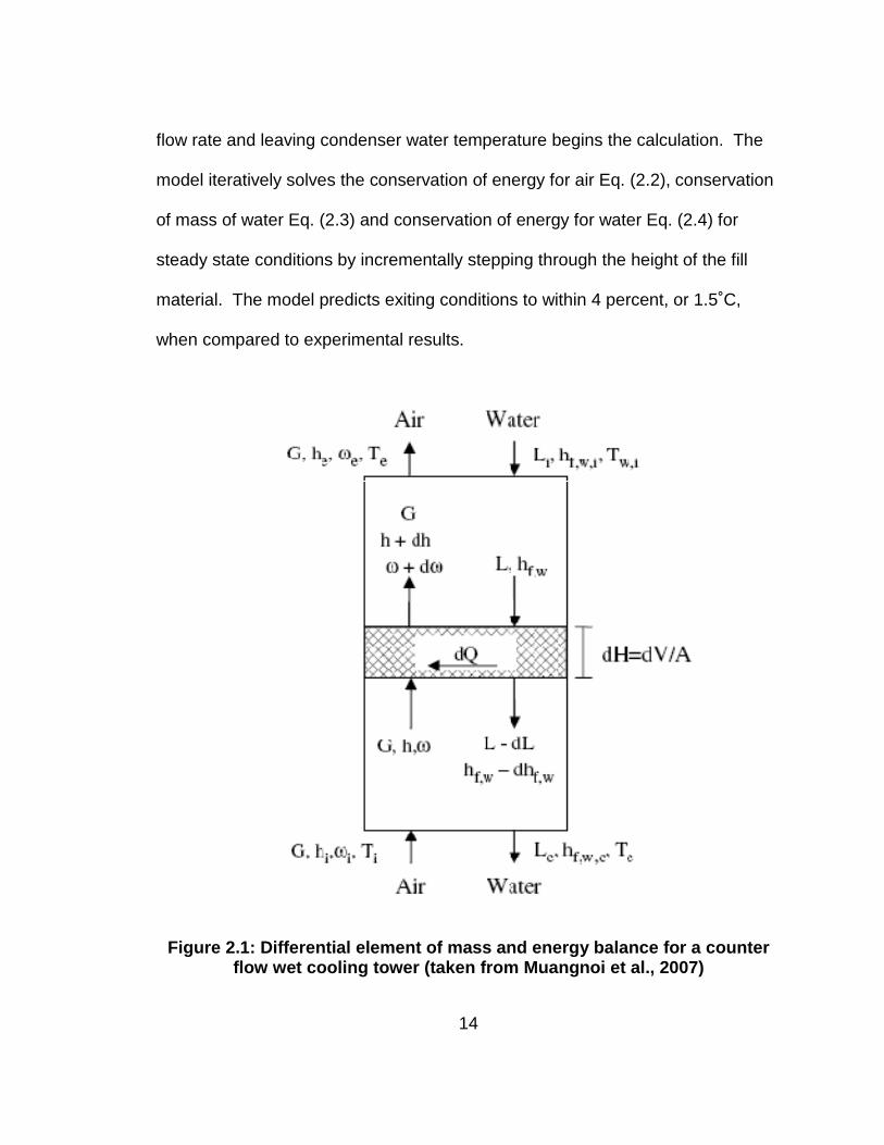
14

flow rate and leaving condenser water temperature begins the calculation. The

model iteratively solves the conservation of energy for air Eq. (2.2), conservation

of mass of water Eq. (2.3) and conservation of energy for water Eq. (2.4) for

steady state conditions by incrementally stepping through the height of the fill

material. The model predicts exiting conditions to within 4 percent, or 1.5˚C,

when compared to experimental results.

Figure 2.1: Differential element of mass and energy balance for a counter flow wet cooling tower (taken from Muangnoi et al., 2007)

15

;< . =>

? @A 7 B C ,D,-, 7 ,EF Eq. (2.2)

G< . =>

? D,-, 7 ,E Eq. (2.3)

*H< . ?

IJ,H D 7 ,,E Eq. (2.4)

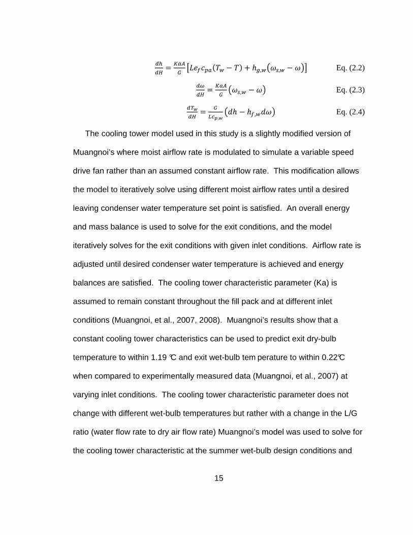
The cooling tower model used in this study is a slightly modified version of

Muangnoi’s where moist airflow rate is modulated to simulate a variable speed

drive fan rather than an assumed constant airflow rate. This modification allows

the model to iteratively solve using different moist airflow rates until a desired

leaving condenser water temperature set point is satisfied. An overall energy

and mass balance is used to solve for the exit conditions, and the model

iteratively solves for the exit conditions with given inlet conditions. Airflow rate is

adjusted until desired condenser water temperature is achieved and energy

balances are satisfied. The cooling tower characteristic parameter (Ka) is

assumed to remain constant throughout the fill pack and at different inlet

conditions (Muangnoi, et al., 2007, 2008). Muangnoi’s results show that a

constant cooling tower characteristics can be used to predict exit dry-bulb

temperature to within 1.19 °C and exit wet-bulb tem perature to within 0.22°C

when compared to experimentally measured data (Muangnoi, et al., 2007) at

varying inlet conditions. The cooling tower characteristic parameter does not

change with different wet-bulb temperatures but rather with a change in the L/G

ratio (water flow rate to dry air flow rate) Muangnoi’s model was used to solve for

the cooling tower characteristic at the summer wet-bulb design conditions and

16

manufacturer data from GEA Power Cooling Incorporated (GEA, 2009). The

Lewis factor is assumed to be unity (Muangnoi, et al., 2007). After the required

air mass flow rate is determined, it is used to estimate fan brake power for the

given inlet conditions. This result simulates a cooling tower with a variable speed

drive (VSD) over a wide range of air inlet conditions.

If the VSD reaches 100 percent and cannot maintain leaving water

temperature set point, then the leaving water temperature is adjusted upward

incrementally until air velocity through the cooling tower fill pack is below 2.5 m/s.

Air flow rate above 2.5m/s will exceed the brake horse power for the fan being

modeled and selected cooling tower make and model. The valid range for air

velocity through a fill pack is between 1.5 m/s to 2.75 m/s for the GEA counter-

flow towers. This is in agreement with ASHRAE’s typical limits of 300 to 700 fpm

(1.5 to 3.5 m/s) (ASHRAE, 2008). Results from this modified component model

are shown in Table 2.1 are nearly within +/- 0.2°C o f Muangoi’s models, which is

within the uncertainty of his model when compared to experimental data.

17

Table 2.1: Predicted conditions for a cooling tower model

Inlet Conditions

Muangnoi et. al.

Predicted Exit Air Conditions Modified Model Predicted Exit

Tdb,i φ (%) Twb,i Tdb,e φ (%) Twb,e G Tdb,e φ (%) Twb,e G

[C] [-] [C] [C] [-] [C] [kg/s] [C] [-] [C] [kg/s]

32.40 40.0 21.92 34.30 98.5 34.08 0.0726 34.32 98.71 34.13 0.0713

32.40 45.0 22.98 34.08 98.0 33.78 0.0806 34.10 98.20 33.84 0.0790

32.40 50.0 23.99 33.82 97.2 33.41 0.0914 33.84 97.46 33.47 0.0894

32.40 55.0 24.96 33.51 96.0 32.92 0.1073 33.53 96.33 32.99 0.1047

32.40 60.0 25.90 33.14 94.1 32.27 0.1271 33.17 94.51 32.35 0.1297

32.40 65.0 26.81 32.73 90.8 31.36 0.1725 32.75 91.34 31.47 0.1799

32.40 70.0 27.69 32.36 84.2 29.99 0.3750 32.37 85.07 30.13 0.3470

27.00 70.0 22.78 33.83 100.0 33.83 0.0788 33.86 100.00 33.86 0.0773

28.00 70.0 23.69 33.58 99.6 33.52 0.0877 33.61 99.76 33.58 0.0859

29.00 70.0 24.60 33.28 98.2 33.02 0.1004 33.32 99.01 33.17 0.0982

30.00 70.0 25.50 32.49 97.4 32.11 0.1205 32.98 97.66 32.64 0.1174

31.00 70.0 26.41 32.58 94.6 31.79 0.1580 32.62 95.00 31.89 0.1528

32.00 70.0 27.32 32.33 88.6 30.64 0.2685 32.35 89.26 30.76 0.2449

2.3 Chiller Component

Chillers mechanically produce chilled water by removing heat from the chilled

water return and rejecting it to the condenser water. The heat is removed by the

cooling tower. Modeling a centrifugal chiller can quickly become complex since

they typically consist of multi-stage compressors, refrigerant economizers,

turning vanes, condenser and evaporator tube bundles, and temperature based

throttling valves. The performance of a chiller is dependent on several operating

factors such as condenser fluid temperature, refrigerant selection, and chilled

water supply temperatures. Typically, negative-pressure chillers (referring to

18

refrigerant below atmospheric pressure) operate at a peak loading of 0.5kW/ton

efficiency or less as opposed to positive-pressure chillers that commonly operate

at 0.55kW/ton efficiency or greater (Standford, 2003).

The capacity of the chiller is determined by a series of tests, rating

requirements, and operating parameters such as 29.4 ºC (85 ºF) entering

condenser water temperature and 6.7 ºC (44 ºF) exiting evaporator water

temperature as shown in Table 2.2 (Air-Conditioning and Refrigeration Institute,

2003). The rated capacities found in supplier catalogs are usually certified

ratings based on Air-Conditioning and Refrigeration Institute (ARI) testing

requirements and not the maximum true capacity. The simulation model requires

the capacity of the chiller to be specified for the given operating range.

Table 2.2: ARI standard rating conditions for a wat er-cooled chiller

ARI Standard Rating Conditions Condenser Evaporator Temperature Entering 85 ˚F Leaving 44 ˚F Flow Rate 3.0 gpm/ton 2.4 gpm/ton Water-side Fouling 0.00025 hr-ft2-˚F/Btu 0.0001 hr-ft2-˚F/Btu

Chiller load is determined based on entering evaporator temperature and

mass flow rate, and exiting chilled water set point. Chiller efficiencies may

increase by 1 to 3 percent for every one degree increase of evaporator water

temperature (Taras, 2005). The chiller efficiency improves when exiting chilled

water evaporator temperatures can be elevated.

Performance parameters for typical centrifugal chillers can be found by curve

fitting a 3rd order polynomial using Microsoft Excel as shown in Figure 2.2 and Eq

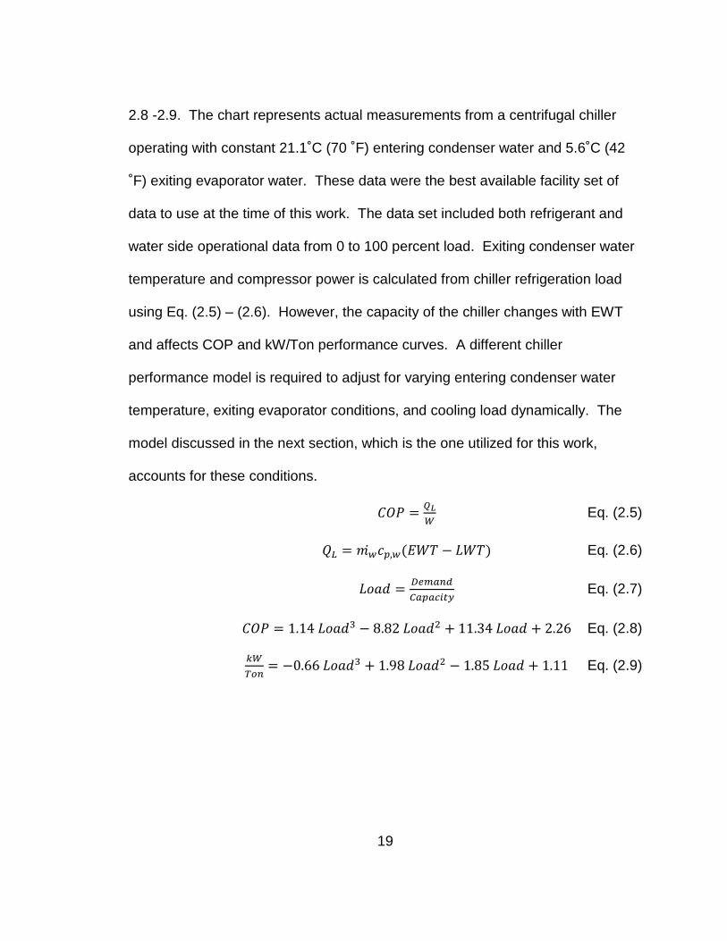
19

2.8 -2.9. The chart represents actual measurements from a centrifugal chiller

operating with constant 21.1˚C (70 ˚F) entering condenser water and 5.6˚C (42

˚F) exiting evaporator water. These data were the best available facility set of

data to use at the time of this work. The data set included both refrigerant and

water side operational data from 0 to 100 percent load. Exiting condenser water

temperature and compressor power is calculated from chiller refrigeration load

using Eq. (2.5) – (2.6). However, the capacity of the chiller changes with EWT

and affects COP and kW/Ton performance curves. A different chiller

performance model is required to adjust for varying entering condenser water

temperature, exiting evaporator conditions, and cooling load dynamically. The

model discussed in the next section, which is the one utilized for this work,

accounts for these conditions.

KLM . NOP Eq. (2.5)

I . Q% ,AR 7 RB Eq. (2.6)

S . TUV!W Eq. (2.7)

KLM . 1.14 S[ 7 8.82 S^ C 11.34 S C 2.26 Eq. (2.8)

P* . 70.66 S[ C 1.98 S^ 7 1.85 S C 1.11 Eq. (2.9)

20

Figure 2.2: Typical chiller performance

For the simulation model, the chiller is modeled using the Simple

Thermodynamic Model (STM) developed by Gordon and Ng (Gordon, Ng, 2000).

The STM has been shown to predict COP within 5 percent using inputs of the

inlet evaporator and condenser temperatures, the power input, and the rate of

heat removal. Additional inputs include the internal entropy generation,

condenser and evaporator thermal resistance, and heat leakage to the

surroundings. Saththasivam and Choon (Saththasivam, Choon, 2008) have

presented methods for determining these latter values for a chiller, and they have

shown them to stay relatively constant for a given chiller.

COP & kW/Ton vs Evaporator Cooling Load70 ˚F Condensor EWT

kW/Ton = -0.6571x3 + 1.975x2 - 1.8452x + 1.1108R² = 0.9366

COP = 1.1435x3 - 8.8221x2 + 11.339x + 2.2624R² = 0.914

0

1

2

3

4

5

6

7

8

9

10

0 0.1 0.2 0.3 0.4 0.5 0.6 0.7 0.8 0.9 1

% Load

CO

P

0

0.1

0.2

0.3

0.4

0.5

0.6

0.7

0.8

0.9

1

kW/T

on

COP KW/Ton Poly. (KW/Ton) Poly. (COP)

21

Operation data were collected from a building management system (BMS) for

a nominal 1,280 ton chiller with a condenser water supply temperature of 70°F,

which is the same chiller used to produce Figure 2.2. STM values for a 1280 ton

centrifugal chiller have been determined utilizing the same technique for curve

fitting COP data and are used as inputs to the current models. Table 2.3 is the

result of modeling Eq. (2.10) – (2.16) using a statistical software package, JMP

(SAS, 2009), to calibrate STM values with measured chiller data. Figure 2.3 is

an overlay plot of measured COP (red square) and the predicted COP (blue

diamond) from the STM model. The graph shows good correlation between

predicted COP by STM and the actual measured COP. The predicted COP

found from the STM model is used to calculate power consumption of the chiller,

Eq. (2.5) – (2.6), for varying loads. Gordon and Ng (Gordon, Ng, 2000) provides

tables for other chiller sizes and types.

22

Figure 2.3: STM predicted COP verses measured COP f or a 1280 ton centrifugal chiller

The STM modeling method can predict COP for several independent

variables that Eq. (2.8) –(2.9) does not include. COP in Eq. (2.10) is a function of

entering evaporator water temperature, entering condenser water temperature,

and cooling load. A new curve would have to be generated for every possible

operating condition to use Eq. (2.8)- (2.9) and would be only valid for the

constant entering condenser water temperature and leaving evaporator

conditions. The STM method is more applicable for this model as entering water

conditions and cooling load will vary with outside air conditions.

3

3.5

4

4.5

5

5.5

6

6.5

7

7.5

20 40 60 80 100

Coe

ffici

ent o

f Per

form

ance

% Load

COP MeasuredCOP Predicted by STM

23

d1 C 1KLMe 7 1

. Δ)* C , f 7

g

C h d1 C 1KLMei

Eq.

(2.10)

j . *9klJ45*m15845 n1 C o

Vpqr 7 1 Eq. (2.11)

$o . *9klJ45N9klJ Eq. (2.12)

$^ . d*m15845 s*9klJ45*m15845 N9klJ e Eq. (2.13)

$[ . N9klJ*m15845 n1 C oVpqr Eq. (2.14)

j . $oΔ)* C $^Quvwx,vyz C $[ Eq. (2.15)

KLM . N9klJq Eq. (2.16)

Table 2.3: Simple thermodynamic model parameters

Parameter Estimate Approximate Standard Error

∆)* 0.9372 kW/K 0.01 kW/K

0.0045 K/kW 2.2E-5 K/kW

Quvwx,vyz -1532 kW 92 kW

2.4 Plate and Frame Heat Exchanger

The plate and frame heat exchanger in the IWE is used to pre-cool the chilled

water return from the data center before entering the evaporator bundle of the

24

chiller. The pre-cooling effect, free-cooling, reduces the amount of chiller work to

produce chilled water. Two types of heat exchangers are recommended for

waterside economizers; plate and frame heat exchangers and shell and tube

(Standford, 2003). Plate and frame heat exchangers can achieve close

approach temperatures between 1°F and 2°F as opposed 2 °F for shell and tube

types. The simulation model uses a plate and frame configuration. The

effectiveness-NTU method was used for modeling plate and frame heat

exchangers is incorporated in the simulation model (Janna, 1998). The overall

heat transfer coefficient, |_S, is assumed to remain constant for all flow rates. In

reality, the overall heat transfer coefficient is a function of Reynolds number in

both hot and cold water streams which will increase or decrease the heat transfer

effectiveness (Croce, D'Agaro, 2002). The exit conditions for both chilled water

and condenser are found through an iterative process. In this simulation, the

heat exchanger is enabled when the inlet condenser water is colder than the

chilled water return from the CRAH by 1.5°C.

Table 2.4 contains the assumed values for the plate and frame heat

exchanger for the IWE model. It is sized to provide full free cooling capability

when condenser water temperature is at 11.4 °C or less, which accounts for the

temperature approach on the heat exchanger. At this condenser water

temperature, the return chilled water temperature can be cooled down to 12.8°C

which enables the chiller to be off.

25

Table 2.4: Plate and frame model parameters

Parameter Value Description N 500 Number of plates

| 2.2 kW/m2-K Overall heat transfer coefficient A 1.5 m2 Surface area of a single plate

A plot of predicted leaving water temperatures is shown in

Figure 2.4 as a function of the temperature difference at the inlets; temperature

difference between chilled water return temperature (T_w[1]) from the RAH and

condenser water supply temperature (T_c[1]) from the cooling tower. Assuming

that the entering chilled water return temperature remains constant, the amount

of heat that can be transferred to the condenser water increases with decreasing

entering condenser water supply temperature.

0500100015002000250030003500400045005000

0

5

10

15

20

25

0 2 4 6 8 10 12

Hea

t Tra

nsfe

r (kW

)

Wat

er T

empe

ratu

re (

C)

Inlet Temperature Difference ( C)

T_w[1] T_w[2] T_c[1] T_c[2] Q (kW)

26

Figure 2.4: Plate and frame heat exchanger performa nce

2.5 Makeup Air Handler

The purpose of the make-up air handler (MUA) is to provide pressurization

and fresh air to the data center (Taras, 2005). The pressurization requirement

helps keep the data center clean of air particles by keeping the space differential

pressure positive in relation to the surrounding space. This ensures that no

outside particles infiltrate the data center space. The MUA simulation model

contains a pre-filter, preheat coil, humidifier, single cooling coil, fan, final filter,

and dampers, as shown in Figure 2.5. A reheat coil is not modeled since the air

will be reheated by the hot return air plenum and narrow temperature and

humidity control is not required. The exiting air from the MUA will mix with the

hot return air from the data center. The preheat section provides sensible heating

through the use of a coil. The humidification section assumes adiabatic

evaporation that will cool the preheated air to the final set condition if the

humidity ratio is below the set point. If needed, the humidified air is cooled to the

final set point. The cooling coil also dehumidifies the air when required. Hourly

weather bin data used for the fresh air in the simulation is from EnergyPlus

Energy Simulation Software (United States Department of Energy, 2008) website

or from HDBinWeather Software (Hana, 2008). Energy required to produce

chilled water, humidification water, and hot water for the MUA are not included

with the analysis and outside of the scope to study the economizer. The the

MUA energy requirements are small compared to the total system energy used.

27

Figure 2.5: Makeup air handler schematic

2.6 Computer Room Air Handler

The primary function of the computer room air handler (CRAH) or return air

handler (RAH) is to provide sensible cooling for the hot return air. However, if

the surface of the cooling coil is below the dew point, dehumidification will occur.

Dry, partially dry, and wet coil surfaces require different calculations, and the

model follows ASHRAE’s recommended calculation procedure (Owen, 2004).

The RAH simulation model consists of a filter, cooling coil, fan, and humidifier

sections. The simulation model for the RAH component assumes no

dehumidification for a 12.8°C (55 °F) high tempera ture chilled water supply

because humidity control is maintained by the MUA. The dew-point of the air is

lower than 12.8°C and therefore will not condense moi sture out the air. If the coil

surface is below the dew point of moist air, the dehumidification process cannot

be ignored in energy and exergy balances. Chilled water demand, or flow rate

and temperature, are set by this component. If the datacenter heat load

increases, then the chilled water flow increases. Figure 2.6 shows a CRAH

Tdb,OSA = 47.37 [F]

RHOSA = 0.2 [-]

Tdb,setpoint = 72 [F]

RHsetpoint = 0.5 [-]

Tdb,1 = 47.4 [F]

Tdb,3 = 83.9 [F]

Tdb,4 = 66.0 [F]

Tdb,5 = 66.0 [F]

Tdb,6 = 67.5 [F]

Tdb,7 = 67.5 [F]Tdb,2 = 47.4 [F]

MAKE-UP AIR HANDLER

Qpreheat = 165038 [Btu/hr] Qcooling,coil = -18 [Btu/hr]

RH7 = 0.380 [-]

Qhumidify = -80318 [Btu/hr]

28

where the cooling coils are removing latent heat and estimates the amount of

condensate.

Figure 2.6: Computer room air handler (CRAH) model

2.7 General Exergy Theory - Air Side

Kanoglu et al. documented sensible cooling and heating, heating with

humidification, cooling with dehumidification, evaporative cooling, and adiabatic

mixing processes (Kanoglu, et al., 2007). Moist air is modeled as a combination

of dry air and water vapor components using ideal gas laws. Engineering

Equation Solver (EES) provides enthalpy and entropy values of moist air from a

property database based on National Institute of Standards and Technology

(NIST) JANAF Thermo-chemical tables (Klein, 2007). Using a property database

Tdb,1 = 78 [F]

Twb,1 = 65.2 [F]

Twb,2 = 56.56 [F]

Tchws = 45 [F]

Tdb,2 = 58.6 [F]

Tchwr = 57.8 [F]

Airflow = 33300 [CFM]

RH2 = 88.5 [-]

Tdp,1 = 58.19 [F]

QT = 877526 [Btu/hr]

QL = 181845 [Btu/hr]

QS = 695681 [Btu/hr]

∆TCHW = 12.8 [F]

Vcondensate,3 = 18.95 [gal/hr]

E = 0.8955 [-]

ME = 0.72 [-]BHP = 7.46 [kW]

FHP = 2.089 [kW]

RH1 = 50.58 [-]

∆Pchw = 87.19 [psia]

Vchws = 150 [gpm]

Tcoil,ave = 51.4 [F]

SHR = 79.3 [%]

30% ASHRAE Filter ESP = 0.3 [inch·WC]

TP = 0.5 [inch·WC]

29

simplifies the following equations without needing to calculate dry air and water

vapor properties separately.

Exergy analysis requires choosing a dead state. The dead state occurs when

the system is in equilibrium with the environment and serves as a reference point

to calculate amount of work potential. Because data centers condition outside air

and reject waste heat to the outside air, the dead state will be the current outdoor

environmental conditions.

Mass Balance for Dry Air:

∑ Q% . ∑ Q% ! Eq. (2.17)

Mass Balance for Water Vapor:

∑ Q% . ∑ Q% ! Eq. (2.18)

Mass Balance for Water Vapor as a Ratio of Dry Air (Assuming no humidification

or dehumidification, , . 0):

∑ Q% , . ∑ Q% ! , Eq. (2.19)

Q% . Q% A, 7 , !B Eq. (2.20)

Energy Balance (Assuming no work, R . 0):

C ∑ Q% . ! C ∑ Q% ! Eq. (2.21)

Entropy Balance:

)% 7 )% ! C )% . 0 Eq. (2.22)

∑ )%N% C ∑ Q% 7 ∑ )%N% ! 7 ∑ Q% ! C )% . 0 Eq. (2.23)

∑ N%

* C ∑ Q% 7 ∑ N%* ! 7 ∑ Q% ! C )% . 0

where: k.boundary Eq. (2.24)

30

Exergy Balance:

∑ N%% C ∑ Q% + 7 ∑ N%% ! 7 ∑ Q% + ! 7 % - . 0 Eq. (2.25)

∑ % n1 7 **r C ∑ Q% + 7 ∑ % ! n1 7 **r 7 ∑ Q% + ! 7 % - . 0

: . S

Eq. (2.26)

Stream Flow Exergy:

( )000 ssThh −−−=ψ Eq. (2.27)

Exergy Destruction:

% -! . )% Eq. (2.28)

Second Law Efficiency (Exergy Efficiency):

& . % 123% 45 . 1 7 % 89:% 45 Eq. (2.29)

2.8 General Exergy Theory – Open Systems

In general, thermal plants are open systems and are not evaluated based on

closed system models. The following set of equations generally governs most

components of the thesis simulation model. In subsequent sections, each piece

of mechanical equipment is uniquely modeled to show how it would perform at

varying conditions.

31

First Law of Thermodynamics:

! 7 ∑ % 7 R% C ∑ Q% 7 ∑ Q% !

: . C #^

2 C

Eq. (2.30)

Second Law of Thermodynamics:

)% . ! 7 ∑ N% 4*4

7 ∑ Q% C ∑ Q% ! 0 Eq. (2.31)

Steady State Exergy Balance

% . ∑ n1 7 **4ro % C ∑ Q% A 7 B 7 ∑ Q% A 7 B ! 7 )%

Eq. (2.32)

2.9 Simulation Modeling

Each mechanical component for the IWE is modeled as a module that

produces output states with given inlet conditions; e.g. air handlers, chillers, coils,

cooling towers, heat exchangers, pumps, etc. The components are linked

together and function as a complete thermal system by connecting the states

through an airflow path or piping distribution. This allows each component to

react to outside air conditions and with other mechanical equipment in the facility

system, much as they would function in a true facility. Currently, a mass flow

balance and corresponding temperature for each state interconnects the thesis

32

model components. The model excludes pressure losses through the piping

distribution and components because the amount of energy loss is negligible

when compared to other energy losses in the system. Each state is calculated at

steady-state conditions.

The main inputs to the simulation model are as follows: hourly weather bin

data, data center heat load, operating set points, and performance characteristics

of each mechanical component. For example, the chiller performance curve is

an input to the model that will determine how much energy the chillers will

consume at partial load conditions. In addition, fan and pump characteristic

curves is implemented in the simulation model. The EES code is included in the

appendix starting on page 69.

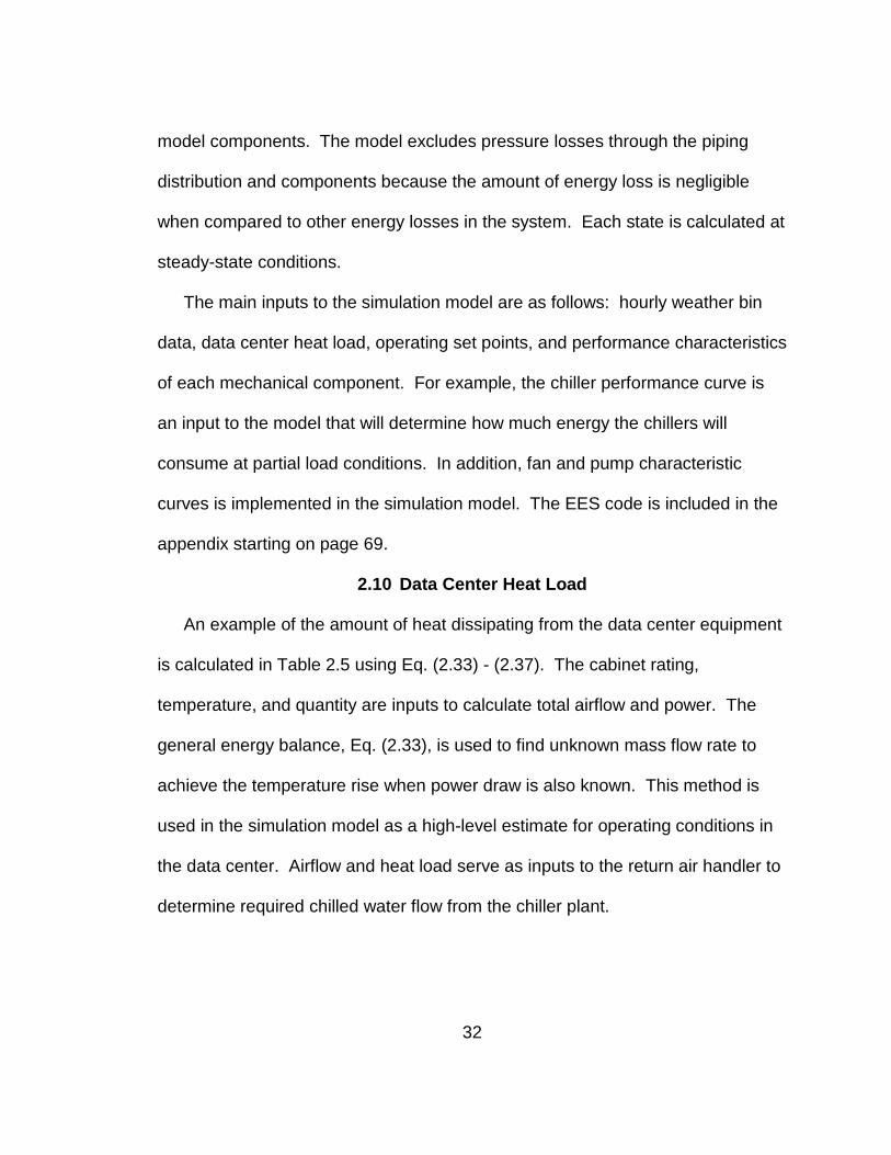
2.10 Data Center Heat Load

An example of the amount of heat dissipating from the data center equipment

is calculated in Table 2.5 using Eq. (2.33) - (2.37). The cabinet rating,

temperature, and quantity are inputs to calculate total airflow and power. The

general energy balance, Eq. (2.33), is used to find unknown mass flow rate to

achieve the temperature rise when power draw is also known. This method is

used in the simulation model as a high-level estimate for operating conditions in

the data center. Airflow and heat load serve as inputs to the return air handler to

determine required chilled water flow from the chiller plant.

33

Table 2.5: Example of data center heat load calcula tions

Cabinet

Description

Cabinet

Rating

Temperature

Rise Quantity CFM/Cabinet Total CFM

Total

Power

[-] [kW] [F] [-] [ft^3/min] [ft^3/min] [kW]

Row 1 HP BLADES 16.5 45 440 1160 510,532 7,260

Row 2 NET APP 7 30 20 738 14,767 140

Not all air supplied from the air handler is used to cool the servers. The

servers will draw in supply air, and excess supply air will bypass the servers and

return to the air handler. The air temperature delta across the RAH coil is less

than the temperature rise across the servers. A bypass flow factor of 20 percent

is applied to the airflow calculations to account for adiabatic mixing. The amount

of air that bypasses the server does vary by air distribution design, where air is

delivered by overhead or under the floor, and can be found using CFD modeling

tools (Herrlin, 2005; Sorell, Abougabal, Khankari, Gandhi, Watve, 2006; Sorell,

Escalante, Yang, 2005). In some cases, air is undersupplied which leads to

virtually no bypass factor but the server inlet conditions are within allowable

specifications. In other cases, more air is supplied than what is required by the

servers to insure inlet temperatures are within the server manufacture’s range or

the data center owner’s allowable range. The air delivered by CRAH can be 80

percent to 120 percent or more of the total server air flow.

34

General Energy Balance:

7 Q% A ! 7 B Eq. (2.33)

inout TTT −=∆ Eq. (2.34)

Volumetric Flow Rate Relationship with Mass and Density:

#% . U% Eq. (2.35)

Volumetric Flow Rate given Heat Dissipation and Change in Temperature:

# . N J¡* Eq. (2.36)

Properties Evaluated at the Average Temperature:

2

inoutave

TTT

+= Eq. (2.37)

2.11 Data Center Facility Modeling Inputs

Additional modeling assumptions have been provided in Table 2.6 that were

used to generate the data set for this analysis. There are many possible

permutations of a facility designs for a data center, and this represents one of

many possible design options. Where possible, equipment sizes such as the

cooling tower, cooling tower fans, and plate and frame heat exchangers, were

cross-referenced with available supplier catalogs (GEA, 2009; Polaris, 2009).

35

Table 2.6: Data center facility modeling inputs

Description Value

Location San Francisco

Data Center Cooling Load 3.8 MW

Total Air Flow 176 m3/s

Qty of Air Handlers 8

Fan Brake Power 25.3kW each

Chilled Water System

Chilled Water Supply Temperature 12.8 °C, 8.9 ∆T

Chilled Water Flow 121.1 l/s

Nominal Chiller Capacity 4.5MW

Cooling Tower, Non Free Cooling

Condenser Water Supply Temperature 17.8 °C, 5.6 ∆T

Condenser Water Flow 212 l/s

Wet-bulb design approach 5.6 °C

Cooling tower characteristic (Ka) 2.219 kg/m3-s

Cooling Tower, Sized for Free Cooling

Wet-bulb design approach 2.2 °C

Approximate Size Relative to Non-Free Cooling 275%

Cooling tower characteristic (Ka) 2.165 kg/m3-s

Data Center Temperature Set point 22.5 +/- 2.5°C

Data Center Relative Humidity Set point 40-55%

There are many permutations of chilled water and condenser water systems

with each of them having their advantages and disadvantages. The modeled

chilled water system is based on a variable primary only flow distribution system.

The condenser water is assumed to be constant flow with variable speed drives

for the fans in the cooling tower. The pump head for both chilled water and

36

condenser water are assumed to be 30.5 m for the simulation. The pump head

is dependent on chilled and condenser water system design, such as pressure

drop through cooling coils, chiller tube bundles, piping scheme, etc. This pump

head value is only used to generate pump power curves for this simulation. The

counter-flow cooling tower requires pressurized nozzles to function verses a

cross-flow tower which does not need spray heads. The cooling tower could be

located on a rooftop with chillers in the basement, which would require more

pumping energy than if the cooling towers were located on the same elevation.

The data center environment is assumed to represent a fully utilized high-

density design with hot aisle containment (Garday, 2007). The hot aisle

containment allows for hotter return air temperatures and potentially increases

the number of partial or full free cooling hours. Each of these assumed values

can be easily changed to run the model under different conditions and for site-

specific design requirements.

37

CHAPTER 3 RESULTS

The EES simulation model calculated energy usage and exergy destroyed for

each mechanical component shown in Figure 1.1 and Figure 1.2. Energy usage

for the MUA and cooling tower in San Francisco is discussed for varying inlet

conditions. As the cooling tower and MUA interact with outdoor air conditions,

the other mechanical equipment adjusts accordingly to the changing conditions.

The energy and exergy plots demonstrate the influence of dry-bulb, wet-bulb,

and relative humidity on mechanical components that do not directly interact,

mix, or share boundaries with the outdoor air.

3.1 Make-up Air Handler

MUA energy requirements have been modeled and trended based on San

Francisco weather bin data. Illustrated in Figure 3.1, the absolute energy of heat

transferred to incoming outside air is plotted from the EES results. Each point in

the chart represents the starting outside conditions for dry bulb temperature and

relative humidity and then the air is conditioned to the required set point

conditions exiting the MUA. The operating set point plus an allowable range

permits the MUA to float with outside air conditions as an energy savings

method. When the set point of 72 ±6°F and 50 +5/-1 0 percent RH was modeled,

as shown in Figure 3.1, the MUA uses the least amount of energy because OSA

conditions are near the set points. Therefore, greater energy savings can be

achieved when the set point operating allowable range is widened. Likewise, the

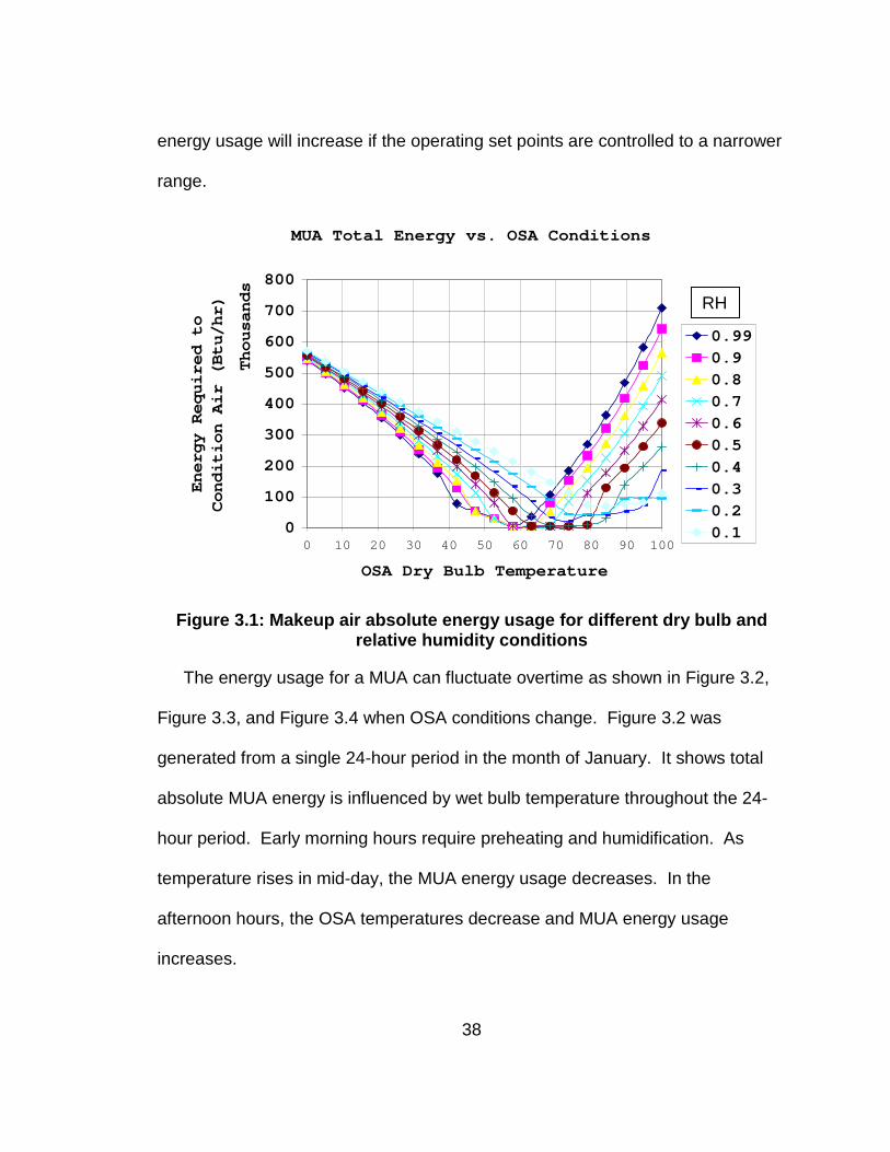
38

energy usage will increase if the operating set points are controlled to a narrower

range.

Figure 3.1: Makeup air absolute energy usage for di fferent dry bulb and relative humidity conditions

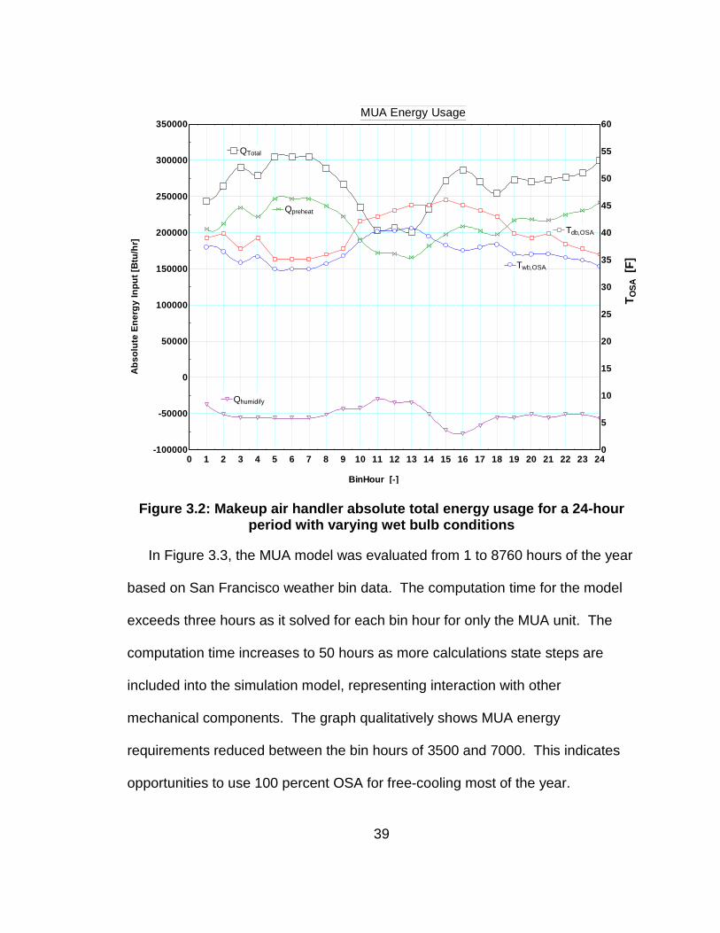
The energy usage for a MUA can fluctuate overtime as shown in Figure 3.2,

Figure 3.3, and Figure 3.4 when OSA conditions change. Figure 3.2 was

generated from a single 24-hour period in the month of January. It shows total

absolute MUA energy is influenced by wet bulb temperature throughout the 24-

hour period. Early morning hours require preheating and humidification. As

temperature rises in mid-day, the MUA energy usage decreases. In the

afternoon hours, the OSA temperatures decrease and MUA energy usage

increases.

MUA Total Energy vs. OSA Conditions

0

100

200

300

400

500

600

700

800

0 10 20 30 40 50 60 70 80 90 100

Thousands

OSA Dry Bulb Temperature

Energy Required to

Condition Air (Btu/hr)

0.99

0.9

0.8

0.7

0.6

0.5

0.4

0.3

0.2

0.1

RH

39

Figure 3.2: Makeup air handler absolute total energ y usage for a 24-hour period with varying wet bulb conditions

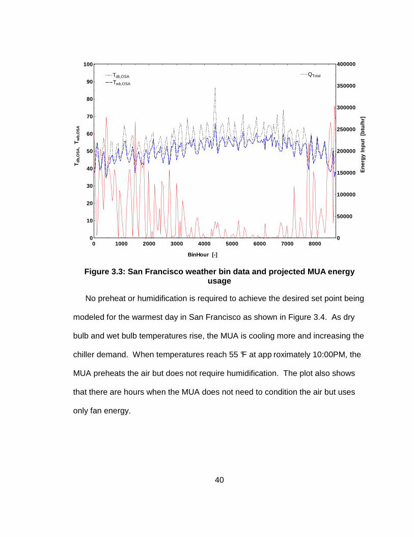
In Figure 3.3, the MUA model was evaluated from 1 to 8760 hours of the year

based on San Francisco weather bin data. The computation time for the model

exceeds three hours as it solved for each bin hour for only the MUA unit. The

computation time increases to 50 hours as more calculations state steps are

included into the simulation model, representing interaction with other

mechanical components. The graph qualitatively shows MUA energy

requirements reduced between the bin hours of 3500 and 7000. This indicates

opportunities to use 100 percent OSA for free-cooling most of the year.

0 1 2 3 4 5 6 7 8 9 10 11 12 13 14 15 16 17 18 19 20 21 22 23 24-100000

-50000

0

50000

100000

150000

200000

250000

300000

350000

0

5

10

15

20

25

30

35

40

45

50

55

60

BinHour [-]

Abs

olut

e E

nerg

y In

put [

Btu

/hr]

QTotalQTotal

TO

SA [

F]

Twb,OSATwb,OSA

MUA Energy Usage

Tdb,OSATdb,OSA

QpreheatQpreheat

QhumidifyQhumidify

40

Figure 3.3: San Francisco weather bin data and proj ected MUA energy usage

No preheat or humidification is required to achieve the desired set point being

modeled for the warmest day in San Francisco as shown in Figure 3.4. As dry

bulb and wet bulb temperatures rise, the MUA is cooling more and increasing the

chiller demand. When temperatures reach 55 °F at app roximately 10:00PM, the

MUA preheats the air but does not require humidification. The plot also shows

that there are hours when the MUA does not need to condition the air but uses

only fan energy.

0 1000 2000 3000 4000 5000 6000 7000 80000

10

20

30

40

50

60

70

80

90

100

0

50000

100000

150000

200000

250000

300000

350000

400000

BinHour [-]

Tdb

,OS

A,

Tw

b,O

SA

Tdb,OSATdb,OSA

Twb,OSATwb,OSA

Ene

rgy

Inpu

t [b

tu/h

r]

QTotalQTotal

41

Figure 3.4: MUA energy transfer on warmest day in S an Francisco

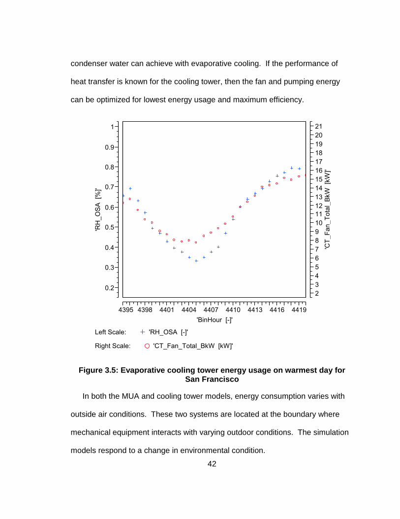
3.2 Cooling Tower

The cooling tower fan energy usage was modeled and was found to vary with

relative humidity as shown in Figure 3.5. The less humid the air, the easier it is

for adiabatic vaporization to occur and requires less air flow. As a result, fan

brake horsepower consumption is reduced. When humidity increases, it

becomes more difficult to evaporate water and therefore more airflow is needed

to evaporate the condenser water. Control logic must be modeled to regulate fan

speed based on exiting condenser water temperature and entering OSA wet-bulb

temperatures. The wet-bulb temperature represents the coldest state that the

4395 4400 4405 4410 4415 44200

5

10

15

20

25

30

35

40

45

50

55

60

65

70

75

80

85

90

-50000

-30000

-10000

10000

30000

50000

BinHour [-]

Tdb

,OS

A,

Tw

b,O

SA

[F

]Tdb,OSATdb,OSA

Twb,OSATwb,OSA

QpreheatQpreheat

QhumidifyQhumidify

Qcooling,coilQcooling,coil

QTotalQTotal

Ene

rgy

[bt

u/hr

]

42

condenser water can achieve with evaporative cooling. If the performance of

heat transfer is known for the cooling tower, then the fan and pumping energy

can be optimized for lowest energy usage and maximum efficiency.

Figure 3.5: Evaporative cooling tower energy usage on warmest day for San Francisco

In both the MUA and cooling tower models, energy consumption varies with

outside air conditions. These two systems are located at the boundary where

mechanical equipment interacts with varying outdoor conditions. The simulation

models respond to a change in environmental condition.

0.2

0.3

0.4

0.5

0.6

0.7

0.8

0.9

1

'RH

_O

SA

[%

]'

2

3

4

5

6

7

8

9

10

11

12

13

14

15

16

17

18

19

20

21

'CT

_F

an

_T

ota

l_B

kW

[k

W]'

4395 4398 4401 4404 4407 4410 4413 4416 4419

'BinHour [-]'

Left Scale: 'RH_OSA [-]'

Right Scale: 'CT_Fan_Total_BkW [kW]'

43

3.3 Economization Hours

The following charts and graphs are the result of running the normal chiller

plant and IWE models developed using Engineering Equation Solver (EES)

(Klein, 2007). A statistical software package, JMP , was utilized to analyze the

data set and determine which parameters have the most influence for a given

variable. Hourly weather bin data used in the simulation is based on San

Francisco, California, USA.

Based on the results of the IWE model and assumed operating set points,

there are 2659 hours/year of full free cooling (chiller completely bypassed) and

6063 hrs/year of partial free cooling. The remaining 38 hours indicate no partial

free cooling is possible because the leaving condenser water temperature from

the cooling tower is greater than the chilled water return temperature from the

CRAH. If the chilled water set point were lower, i.e. 7.2 °C versus 12.7°C, then

the number of full free cooling hours is reduced to around 322 hours/year, 7334

partial free cooling hours/year, and full load on the chiller for 1104 hours/year.

Therefore, choosing the right set points, elevating chilled water return

temperatures, can significantly influence the number of available economizer

hours.

3.4 Energy Consumption

Table 3.1 estimates the power consumption for this system design scenario if

the economizer were off throughout the year. The data center load was

assumed constant. However, in real world operation this would vary. Since the

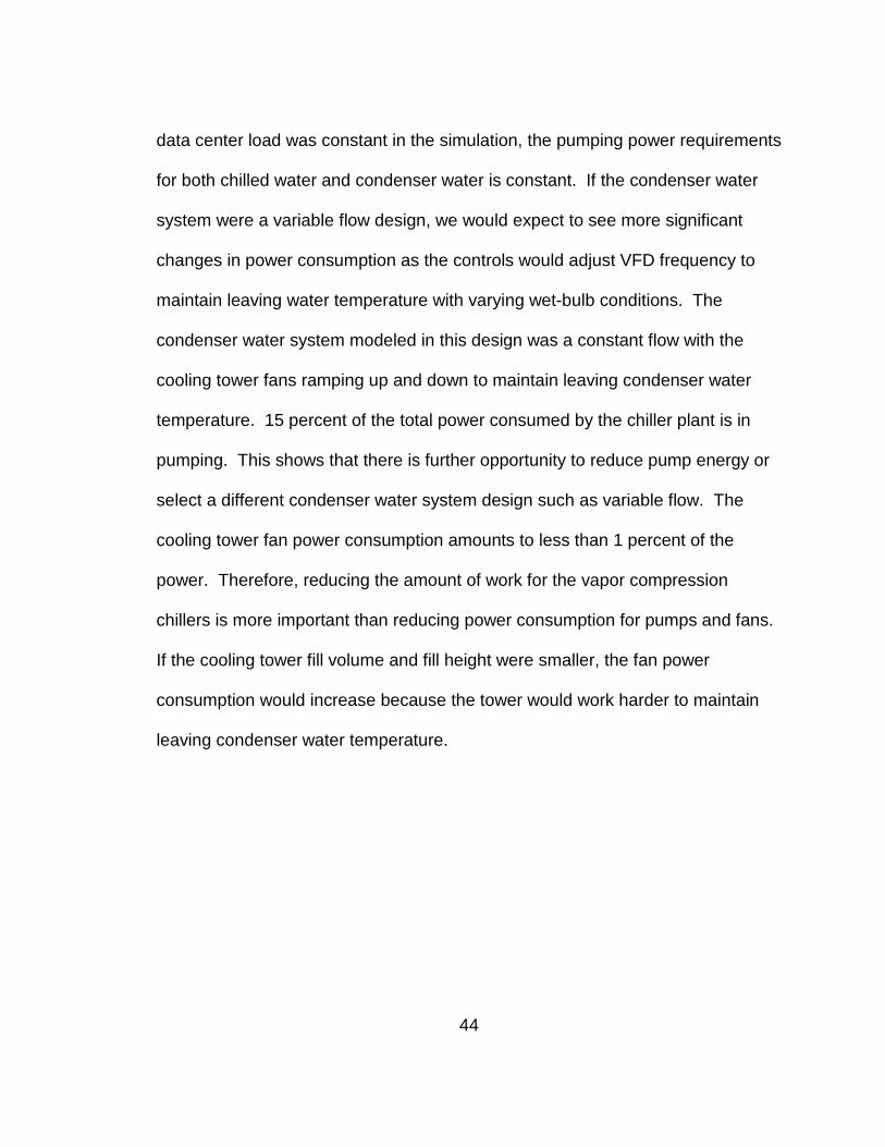
44

data center load was constant in the simulation, the pumping power requirements

for both chilled water and condenser water is constant. If the condenser water

system were a variable flow design, we would expect to see more significant

changes in power consumption as the controls would adjust VFD frequency to

maintain leaving water temperature with varying wet-bulb conditions. The

condenser water system modeled in this design was a constant flow with the

cooling tower fans ramping up and down to maintain leaving condenser water

temperature. 15 percent of the total power consumed by the chiller plant is in

pumping. This shows that there is further opportunity to reduce pump energy or

select a different condenser water system design such as variable flow. The

cooling tower fan power consumption amounts to less than 1 percent of the

power. Therefore, reducing the amount of work for the vapor compression

chillers is more important than reducing power consumption for pumps and fans.

If the cooling tower fill volume and fill height were smaller, the fan power

consumption would increase because the tower would work harder to maintain

leaving condenser water temperature.

45

Table 3.1: Basic chiller plant estimated power cons umption (kWh)

Bin Month Hours CHW PMP CRAH

Cooling

Tower CW PMP MAH Chiller

DC Cooling

Load

COP for

Chiller

Plant

January 744 21,182 20,237 5,258 55,934 4,161 388,371 2,834,640 6.0

February 672 19,132 18,278 6,909 50,521 3,758 351,045 2,560,320 6.0

March 744 21,182 20,237 6,398 55,934 4,161 388,389 2,834,640 6.0

April 720 20,498 19,584 7,894 54,130 4,027 376,161 2,743,200 6.0

May 744 21,182 20,237 10,769 55,934 4,161 390,183 2,834,640 5.9

June 720 20,498 19,584 11,874 54,130 4,027 378,637 2,743,200 5.9

July 744 21,182 20,237 13,775 55,934 4,161 393,290 2,834,640 5.9

August 744 21,182 20,237 14,509 55,934 4,161 394,243 2,834,640 5.8

September 720 20,498 19,584 13,884 54,130 4,027 382,604 2,743,200 5.8

October 744 21,182 20,237 12,825 55,934 4,161 391,384 2,834,640 5.9

November 720 20,498 19,584 9,342 54,130 4,027 376,168 2,743,200 6.0

December 744 21,182 20,237 6,010 55,934 4,161 388,404 2,834,640 6.0

8,760 249,397 238,272 119,448 658,577 48,995 4,598,879 33,375,600 5.9

The estimated energy consumption for the IWE model is shown in Table 3.2.

The same EES model was used to generate Table 3.1 with the exception of the

economizer mode being enabled and a larger cooling tower. One important item

to note is that the energy used to produce chilled water, heating water, and

humidification for the MAH is not included with the MAH values provided in Table

3.1. They are assumed to be supplied from different systems and currently are

outside the scope of the economizer system being studied. In general, the

energy consumption for the MAH is much smaller than the chiller plant and is

ignored. Figure 3.4 shows the cooling load for the MAH to be about 4.2 Tons

(15kW) , which is less than 5 percent of the power consumed by one chiller in

this simulation model. The power represented in Table 3.1 for the MAH is only

fan power. Future revisions of the EES model may be revised to add more detail

for a complete energy model of an operating facility, including compressed air for

46

controls and boilers for hot water. The chilled water produced for the MAH

requires a colder supply temperature, i.e., less than 7.2°C for dehumidification,

verses 12.7 °C sensible only cooling. The chilled water supply temperature for

this analysis assumes 12.7 °C.

Table 3.2: Estimated power consumption with an inte grated wet-side economizer (kWh)

Bin Month Hours

CHW

PMP CRAH

Cooling

Tower CW PMP MAH Chiller

DC Cooling

Load

COP for

Chiller

Plant

January 744 21,162 20,237 7,804 55,934 4,161 44,007 2,834,640 21.3

February 672 19,117 18,278 9,730 50,521 3,758 94,077 2,560,320 14.4

March 744 21,163 20,237 10,084 55,934 4,161 70,661 2,834,640 17.5

April 720 20,483 19,584 11,328 54,130 4,027 112,402 2,743,200 13.6

May 744 21,170 20,237 11,488 55,934 4,161 177,635 2,834,640 10.5

July 744 21,174 20,237 10,226 55,934 4,161 242,296 2,834,640 8.5

August 744 21,175 20,237 9,720 55,934 4,161 249,386 2,834,640 8.3

June 720 20,489 19,584 10,837 54,130 4,027 211,920 2,743,200 9.1

September 720 20,492 19,584 9,274 54,130 4,027 244,675 2,743,200 8.2

October 744 21,173 20,237 10,951 55,934 4,161 221,567 2,834,640 9.0

November 720 20,486 19,584 10,329 54,130 4,027 137,192 2,743,200 12.1

December 744 21,164 20,237 8,949 55,934 4,161 71,226 2,834,640 17.6

8,760 249,249 238,272 120,719 658,577 48,995 1,877,044 33,375,600 11.3

3.5 Energy Efficiency

COP is calculated for the chiller plant as the total data center cooling load

divided by total power consumed by the chiller plant. An average yearly COP

was found to be 11.3 for the IWE design and 5.9 without an economizer. As

expected, power consumption to provide useful cooling is reduced in colder

months compared to the summer months because the economizer is pre-cooling

the return water prior to reaching the chiller, effectively reducing amount of

compressor work for the chiller. Cooling tower fan energy is increased in the

47

IWE because more air is required to provide cold condenser water temperature

with a smaller approach temperature to the wet-bulb. Approach temperature is

the difference between leaving condenser water temperature and entering wet-

bulb temperature.

A common metric used to measure chilled water plant efficiency is kW/ton or

electrical power required per unit of useful cooling. It is the sum of all electrical

power used by the chiller plant divided by the amount of useful cooling generated

in the evaporator of the chiller. The lower the kW/ton or kW/kW results in higher

energy efficiency. Figure 3.6 is a plot of calculated energy efficiency as a

function of dry-bulb temperature for all 8760 hours of the year.

Figure 3.6: Chiller plant with an integrated indire ct wet-side economizer energy efficiency performance (kW/ton) versus outsi de air dry-bulb

temperature

0

0.1

0.2

0.3

0.4

0.5

0.6

0.7

En

erg

y E

ffici

en

cy (

kW/to

n)

0 10 20 30 40

Dry-bulb Temperature (°C)

Full Free Cooling

No Free Cooling

Partial Free Cooling

Bin

0.175

0.275

0.375

0.475

0.575

0.675

0.775

0.875

0.975

RH

48

Figure 3.6 shows that the economizer is very efficient when the

economizer is enabled, full or partial. In full free cooling mode, only the pump

and fan energy is used to transport heat from the data center to the environment.

The energy efficiency was less than 0.15kW/ton in full free cooling mode. This

value represents the best case scenario if nothing else in the chiller plant were

required to operate. The 0.15kW/ton does not include ancillary loads to support

the chiller plant, such as conditioning the chiller room (if required), controls,

refrigerant oil heaters, and redundant chillers in standby. Ideally, full free cooling

is the preferred mode of operation year round, but it is not physically possible

because chilled water cannot be produced without the assistance of the vapor

compression chiller.

Figure 3.7 is a plot of calculated energy efficiency as a function of wet-bulb

temperature. Figure 3.7 shows the same data as Figure 3.6. The wet-bulb

temperature can be found using dry-bulb temperature and relative humidity. It

shows that there is a strong relationship between wet-bulb temperature and

chiller plant kW/ton performance. The wet-bulb temperature can be used to

predict evaporative chiller plant performance better than knowing dry-bulb

temperature and relative humidity as separate variables.

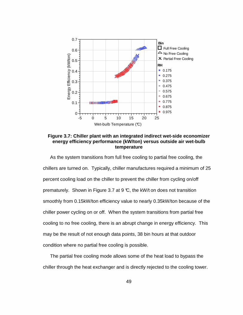
49

Figure 3.7: Chiller plant with an integrated indire ct wet-side economizer energy efficiency performance (kW/ton) versus outsi de air wet-bulb

temperature

As the system transitions from full free cooling to partial free cooling, the

chillers are turned on. Typically, chiller manufactures required a minimum of 25

percent cooling load on the chiller to prevent the chiller from cycling on/off

prematurely. Shown in Figure 3.7 at 9 °C, the kW/t on does not transition

smoothly from 0.15kW/ton efficiency value to nearly 0.35kW/ton because of the

chiller power cycling on or off. When the system transitions from partial free

cooling to no free cooling, there is an abrupt change in energy efficiency. This

may be the result of not enough data points, 38 bin hours at that outdoor

condition where no partial free cooling is possible.

The partial free cooling mode allows some of the heat load to bypass the

chiller through the heat exchanger and is directly rejected to the cooling tower.

0

0.1

0.2

0.3

0.4

0.5

0.6

0.7

Ene

rgy

Effi

cien

cy (

kW/to

n)

-5 0 5 10 15 20 25

Wet-bulb Temperature (°C)

Full Free Cooling

No Free CoolingPartial Free Cooling

Bin

0.175

0.275

0.3750.475

0.575

0.675

0.775

0.8750.975

RH

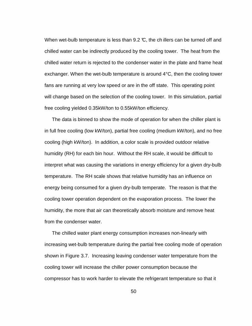
50

When wet-bulb temperature is less than 9.2 °C, the ch illers can be turned off and

chilled water can be indirectly produced by the cooling tower. The heat from the

chilled water return is rejected to the condenser water in the plate and frame heat

exchanger. When the wet-bulb temperature is around 4°C, then the cooling tower

fans are running at very low speed or are in the off state. This operating point

will change based on the selection of the cooling tower. In this simulation, partial

free cooling yielded 0.35kW/ton to 0.55kW/ton efficiency.

The data is binned to show the mode of operation for when the chiller plant is

in full free cooling (low kW/ton), partial free cooling (medium kW/ton), and no free

cooling (high kW/ton). In addition, a color scale is provided outdoor relative

humidity (RH) for each bin hour. Without the RH scale, it would be difficult to

interpret what was causing the variations in energy efficiency for a given dry-bulb

temperature. The RH scale shows that relative humidity has an influence on

energy being consumed for a given dry-bulb temperate. The reason is that the

cooling tower operation dependent on the evaporation process. The lower the

humidity, the more that air can theoretically absorb moisture and remove heat

from the condenser water.

The chilled water plant energy consumption increases non-linearly with

increasing wet-bulb temperature during the partial free cooling mode of operation

shown in Figure 3.7. Increasing leaving condenser water temperature from the

cooling tower will increase the chiller power consumption because the

compressor has to work harder to elevate the refrigerant temperature so that it

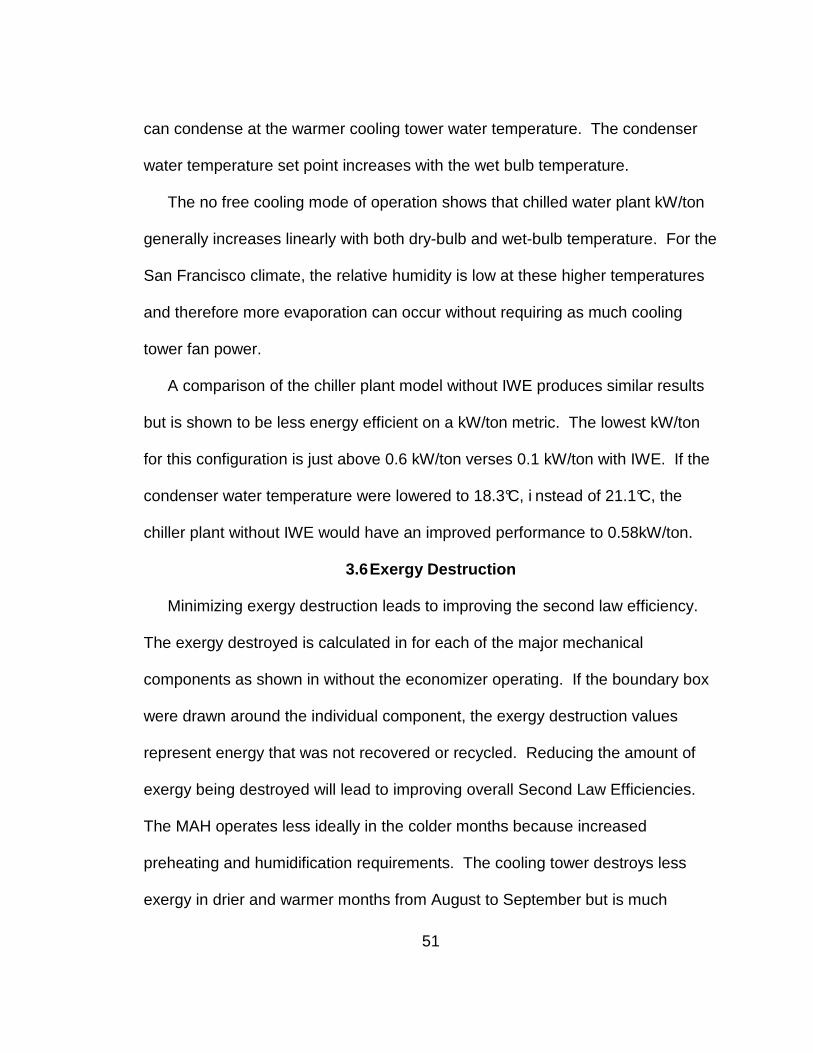
51

can condense at the warmer cooling tower water temperature. The condenser

water temperature set point increases with the wet bulb temperature.

The no free cooling mode of operation shows that chilled water plant kW/ton

generally increases linearly with both dry-bulb and wet-bulb temperature. For the

San Francisco climate, the relative humidity is low at these higher temperatures

and therefore more evaporation can occur without requiring as much cooling

tower fan power.

A comparison of the chiller plant model without IWE produces similar results

but is shown to be less energy efficient on a kW/ton metric. The lowest kW/ton

for this configuration is just above 0.6 kW/ton verses 0.1 kW/ton with IWE. If the

condenser water temperature were lowered to 18.3°C, i nstead of 21.1°C, the

chiller plant without IWE would have an improved performance to 0.58kW/ton.

3.6 Exergy Destruction

Minimizing exergy destruction leads to improving the second law efficiency.

The exergy destroyed is calculated in for each of the major mechanical

components as shown in without the economizer operating. If the boundary box

were drawn around the individual component, the exergy destruction values

represent energy that was not recovered or recycled. Reducing the amount of

exergy being destroyed will lead to improving overall Second Law Efficiencies.

The MAH operates less ideally in the colder months because increased

preheating and humidification requirements. The cooling tower destroys less

exergy in drier and warmer months from August to September but is much

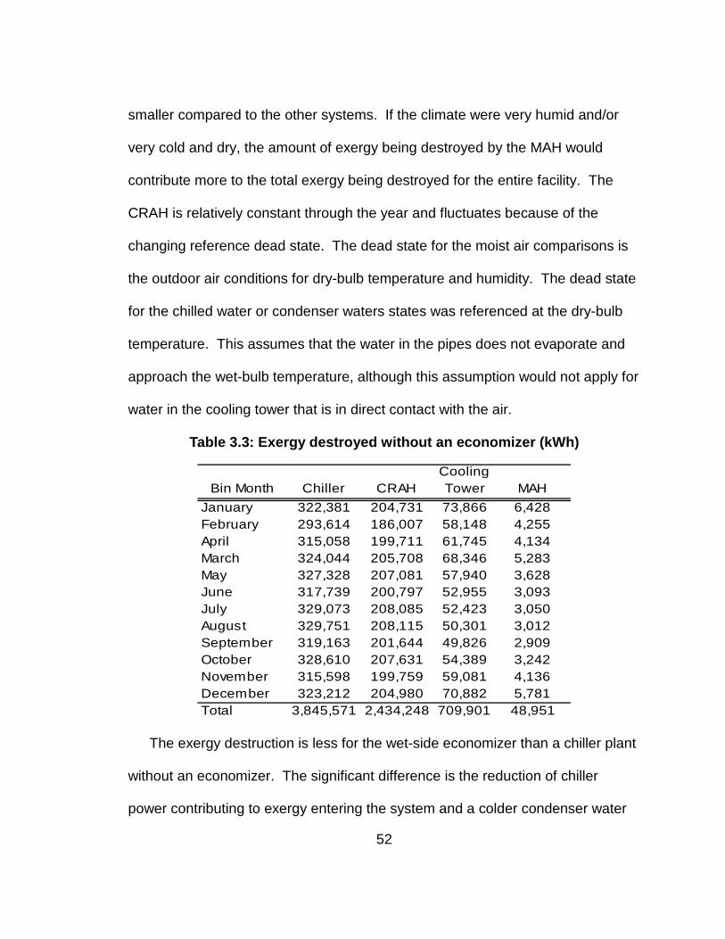
52

smaller compared to the other systems. If the climate were very humid and/or

very cold and dry, the amount of exergy being destroyed by the MAH would

contribute more to the total exergy being destroyed for the entire facility. The

CRAH is relatively constant through the year and fluctuates because of the

changing reference dead state. The dead state for the moist air comparisons is

the outdoor air conditions for dry-bulb temperature and humidity. The dead state

for the chilled water or condenser waters states was referenced at the dry-bulb

temperature. This assumes that the water in the pipes does not evaporate and

approach the wet-bulb temperature, although this assumption would not apply for

water in the cooling tower that is in direct contact with the air.

Table 3.3: Exergy destroyed without an economizer (k Wh)

Bin Month Chiller CRAHCooling Tower MAH

January 322,381 204,731 73,866 6,428February 293,614 186,007 58,148 4,255April 315,058 199,711 61,745 4,134March 324,044 205,708 68,346 5,283May 327,328 207,081 57,940 3,628June 317,739 200,797 52,955 3,093July 329,073 208,085 52,423 3,050August 329,751 208,115 50,301 3,012September 319,163 201,644 49,826 2,909October 328,610 207,631 54,389 3,242November 315,598 199,759 59,081 4,136December 323,212 204,980 70,882 5,781Total 3,845,571 2,434,248 709,901 48,951

The exergy destruction is less for the wet-side economizer than a chiller plant

without an economizer. The significant difference is the reduction of chiller

power contributing to exergy entering the system and a colder condenser water

53

temperature leaving the cooling tower. In the IWE model, the CRAH destroys

more exergy on a yearly average than the chiller. This occurs because of the

large temperature differences between the air and chilled water as heat is

transferred from the air to the chilled water, and the chiller power consumption is

reduced because of the economizer. Under these conditions, improving the

efficiency of the CRAH becomes as important as reducing cooling load on the

chiller as found in the energy only analysis. The exergy results show reducing

exergy destruction with CRAH is an area of important focus to minimize exergy

being destroyed if the chiller plant already has an economizer.

In both models, the total exergy destroyed for the CRAH is nearly the same.

The differences are from a minor change in chilled water temperature return

below exiting the plate and frame heat exchanger. In some cases, the chilled

water supply temperature was colder than in the model with the economizer

turned off. The exergy for the cooling tower is less in the IWE model because of

the closer approach assumption for leaving condenser water temperature and its

system temperature is operating closest to the outside air conditions; exergy

entering on the airside of the cooling tower is zero because it is already at the

dead state. In the model without the economizer, the leaving condenser water

was constant for the majority of the year with the exception when the condenser

water temperature was adjusted to a higher leaving water temperature set point

because the approach exceeded the design of the cooling tower. The heat

exchanger destroys exergy also because the heat transfer process generates

54

entropy. Most of the entering exergy is recovered but the temperature

differences between the condenser water and chilled water still causes exergy to

be destroyed. This indicates that heat transfer between fluids across boundaries

should be reduced as much as possible in the facility design or as differential

temperature between hot and cold should approach zero degrees, which is not

practical because of a very large heat exchanger. Some exergy destroyed

because of heat transfer is not that important since in reality it will never be

recovered. This may be an indicator that for the same climate, a direct wet-side

economizer might destroy less exergy because the chiller and heat exchanger

are eliminated during full free cooling mode. The exergy destroyed by the MAH

in the IWE is exactly the same as the model with the economizer turned off.

Table 3.4: Exergy destroyed with an economizer (kWh)

Bin Month Chiller CRAHCooling Tower

Heat Exchanger MAH

January 41,657 207,755 36,554 29,388 6,428February 88,239 187,700 29,367 23,972 4,255March 66,959 208,196 34,796 28,677 5,283April 105,475 201,286 33,608 25,334 4,134May 162,948 207,773 32,832 20,348 3,628June 193,148 200,898 30,644 16,364 3,093July 217,121 208,085 31,383 12,945 3,050August 221,699 208,115 29,610 11,063 3,012September 216,564 201,663 30,833 10,243 2,909October 201,089 207,764 32,625 15,917 3,242November 126,939 200,984 31,389 22,170 4,136December 67,388 207,395 35,400 28,327 5,781Total 1,709,226 2,447,614 389,041 244,748 48,951

Figure 3.8 shows that exergy destruction increases with lower humidity, but

second law efficiency increases as well. Although counter-intuitive, this is

55

because the sum of the rates of exergy entering the components has increased

more than the increase in rate of exergy destroyed, leading to an increase in

efficiency. More cooling tower water is being evaporated, which increases the

amount of makeup water exergy entering the system, but fan energy has been

reduced. The exergy destroyed in these figures is for the CRAH, MAH cooling

tower, cooling tower makeup, data center air leakage, chiller, and heat

exchanger.

The exergy destruction is plotted for all bin hours. Exergy destruction is

minimized for the system in Figure 3.8 when the cooling tower exergy destruction

is at its minimum. This occurs when the wet-bulb temperature is near 9.2°C and

when the economizer is in full free cooling mode. When the wet-bulb

temperature is greater than 9.2°C, the economizer swi tches from full to partial

free cooling. The higher relative humidity corresponds to a larger wet-bulb

temperature at the same dry-bulb temperature. The current condenser water

temperature adjusts its set point to a higher temperature because the leaving

cooling tower water is unable to maintain leaving water temperature. This occurs

because the evaporation process is not removing enough heat to adequately

cool down the leaving water to the set point. In partial free cooling, the exergy

destruction increases non-linearly with increasing dry-bulb similarly for the same

reason as that shown than in Figure 3.8 for the partial free cooling mode.

Increasing the temperature of the condenser water entering the chiller also

increases the work for the chiller and therefore energy efficiency decreases.

56

The STM model accounts for efficiency losses with elevating condenser water

temperature and decreasing chilled water return temperature. Figure 3.8 also

shows that it actually may be beneficial to switch over from partial free cooling to

no free cooling mode sooner to reduce the amount of exergy being destroyed.

Figure 3.8: Total exergy destroyed versus outdoor d ry-bulb temperature for chilled water plant with IWE

The 2nd Law efficiency is calculated for each bin hour of the year in Figure

3.9. Each mode of operation for the economizer has its most efficient and least

efficient operating point. The full free cooling mode has its best efficiency of 56

percent when moist air conditions are cold and dry, 15.6°C dry-bulb and 20

percent RH. When the economizer switches from full to partial free cooling mode

at about 9°C wet-bulb, system efficiency noticeably dro ps because the chiller is

operating to produce chilled water to meet the desired chilled water supply

300

400

500

600

700

800

900

1000

De

stro

yed

(kW

h)

0 10 20 30 40

Dry-bulb Temperature (°C)

Full Free Cooling

No Free Cooling

Partial Free Cooling

Bin

0.175

0.275

0.375

0.475

0.575

0.675

0.775

0.875

0.975

RH

Dry-Bulb Temperature (°C)

57

temperature set point. When no free cooling is possible at higher wet-bulb

temperature, the average efficiency drops again but this represents only 38 hours

of data points. Further research is required to show that an economizer can be

controlled by maximizing 2nd Law Efficiency, but it may be easier to use exergy

destroyed calculations to optimize the economizer system.

Figure 3.9: 2nd Law efficiency plot for wet-bulb te mperature for chilled water plant with IWE

0

0.1

0.2

0.3

0.4

0.5

0.6

0.7

2n

d L

aw

Effi

cien

cy

-5 0 5 10 15 20 25

Wet-bulb Temperature (°C)

Full Free Cooling

No Free Cooling

Partial Free Cooling

Bin

0.175

0.275

0.375

0.475

0.5750.675

0.775

0.875

0.975

'RH_OSA [-]'

58

CHAPTER 4 CONCLUSION

A simulation model for predicting the response of a chiller plant with an

economizer was developed to investigate where the most exergy was destroyed

and where most energy was consumed for every hour of the year. For a chiller

plant operating with an economizer, the CRAH was the largest source for exergy

destruction. For a chiller plant operating without an economizer, the chiller was

the largest source for exergy destruction. In addition, it was shown that Second

Law efficiencies would vary significantly throughout a given year in San

Francisco.

According to the 1st Law of Thermodynamics, reducing the amount of

parasitic losses, such as friction, will make mechanical components more energy

efficient. Since electrical power consumed is exergy destroyed, reducing overall

energy consumption will minimize exergy destruction.

Second Law analysis will indicate when, where, and how the exergy is

destroyed. Reducing the amount of heat transfer between fluids and reducing

the temperature difference should reduce the amount of exergy destroyed in the

system since entropy is a function of energy transferred and effective boundary

temperatures. For the outside air economizer, indoor air is directly mixed with

outside air. This eliminates one more energy transfer between system

boundaries. This may be an indication that a system with an outside air

economizer will yield the least amount of exergy destroyed.

59

4.1 Future Work

Additional simulation models should be developed to compare energy and

exergy results other designs, such as OAE and DWE, for other climates. The

exergy analysis may show which type of economizer is suited best for a given

climate. The programming environment that EES provides, easy access to fluid

properties, allows engineers to quickly evaluate designs and predict performance

of a system under varying conditions. Listed below are a few areas that could

improve the simulation model:

1. Modify cooling coil algorithms for partial and wet surfaces to account for

the dehumidification process.

2. Modify plate and frame heat exchanger calculations to adjust heat transfer

coefficients based on changes with the Reynold’s number, because flow

rates and temperatures are not constant.

3. Modify MUA and RAH for OSA economizer operation.

4. Expand simulation for a DWE system.

5. Expand energy and exergy analysis for supporting systems that were

excluded from this analysis such as the hot water system.

6. Improve the solver calculation method to use a technique other than the

Newton-Raphson technique.

60

REFERENCES

Air-Conditioning and Refrigeration Institute (2003) ARI 550/590-2003: performance rating of water chilling packages using the vapor compression cycle. Retrieved from http://www.ari.org

Aprea, C., Rossi, F. d., Greco, A., Renno, C. (2003) Refrigeration plant exergetic analysis varying the compressor capacity. International Journal of Energy Research 27(7), 653-669.

ASHRAE (2008) HVAC systems and equipment ASHRAE Handbook (pp. 39.19).

Bejan, A. (2006) Advanced engineering thermodynamics (3rd ed.): John Wiley & Sons, Inc.

Bejan, A., Tsatsaronis, G., Moran, M. (1996) Thermal design and optimization: John Wiley & Sons, Inc.

Cengel, Y. A., Boles, M. A. (2006) Thermodynamics: an engineering approach, 5th edition: McGraw Hill.

Chen, C. K., Su, Y. F. (2005) Application of exergy method to an irreversible inter-cooled refrigeration cycle. Proceedings of the Institution of Mechanical Engineers, Part A, Power & Energy 219(8), 661-667.

Chen, C. K., Su, Y. F. (2006) Exergetic efficiency optimization of a refrigeration system with multi-irreversibilities. Proceedings of the Institution of Mechanical Engineers, Part C, Journal of Mechanical Engineering Science 220(8), 1179-1187.

Chen, C. K., Su, Y. F. (2007) Application of exergy method to a two-stage irreversible combined refrigeration system. Proceedings of the Institution of Mechanical Engineers, Part C, Journal of Mechanical Engineering Science 221(7), 807-813.

61

Croce, G., D'Agaro, P. (2002) Numerical analysis of forced convection in plate and frame heat exchangers. International Journal of Numerical Methods for Heat and Fluid Flow 12, 756-771.

Department of Planning and Development (2006) Washington State Non-residential Energy Code Retrieved from http://www.seattle.gov/DPD/Codes/Energy_Code/Nonresidential/Chapter_14/default.asp.

Dincer, I., Hussain, M. M., Zubair, S. M. (2004) A feasibility study of using thermal energy storage in a conventional air-conditioning system. International Journal of Energy Research 28(11), 955-967.

Fisk, W. J., Seppänen, O., Faulkner, D., Huang, J. (2005) Economic benefits of an economizer system: energy savings and reduced sick leave. ASHRAE Transactions 111(2), 673-679.

Garday, D. (2007) Reducing data center energy consumption with wet side economizers Intel Information Technology White Paper.

GEA (2009). Cooling tower calculator Retrieved 1/18/2009, from http://gea-energytechnology.com/opencms/opencms/gem/en/calculators/CT_Calculator.html

Gordon, J. M., Ng, K. C. (2000) Cool thermodynamics: the engineering and physics of predictive, diagnostic and optimization methods for cooling systems: Cambridge International Science Publishing.

Greenberg, S. (2007) Data center energy use, metrics, and rating systems. ENERGY STAR Industry Focus Discussion: Development of Energy Performance Benchmark for Data Centers, (October 31, 2007). Retrieved from http://www.energystar.gov/ia/partners/prod_development/downloads/DC_Energy_Metrics.pdf

Hana, B. (2008) HDBinWeather: Hands Down Software.

62

Harutunian, V. (2003) Functional model and second law analysis method for energy efficient process design: applications in HVAC systems design. Ph.D., The University of Texas at Austin, Texas, United States. Retrieved from http://proquest.umi.com/pqdweb?did=765218911&

Hasabnis, Y. C., Bhagwat, S. S. (2007) Performance evaluation of ammonia absorption refrigeration cycle based on exergetic coefficient of performance. International Journal of Exergy 4(1), 19-37.

Herrlin, M. K. (2005) Rack cooling effectiveness in data centers and telecom central offices: the rack cooling index (RCI). Paper presented at the American Society of Heating, Refrigerating and Air-Conditioning Engineers, ASHRAE 2005 Annual Meeting, June 25, 2005 - June 29, 2005, Denver, CO, United States.

Imperatore, T. (1975) Proven ways to save energy in commercial buidlings. Heating, Piping & Air Conditioning 47(5), 48-53.

Janna, W. S. (1998) Design of fluid thermal systems (2nd ed.): PWS Publishing Company.

Kanoglu, M., Dincer, I., Rosen, M. A. (2007) Exergy analysis of psychrometric processes for HVAC&R applications. ASHRAE Transactions 113(2), 172-180.

Klein, S. A. (2007) Engineering Equations Solver (EES): F-Chart Software. Retrieved from www.fchart.com

Koomey, J. G. (2004, March 2, 2004) Data center power use: a review of the historical data. Paper presented at the IBM Austin Conference on Energy-Efficient Design, Austin, Texas.

Kotas, T. J. (1995) The exergy method of thermal plant analysis: Krieger Publishing Company.

Kurkjian, C., Glass, J., Routsen, G. (2007) Efficiency plus reliability. ASHRAE Journal 49(12), 26-31.

63

Li, N., Ren, C., Tang, G., Zhang, G., Yang, J. (2001) Exergy analysis of moist air and energy saving potential in HVAC by evaporative cooling or energy recovery. Paper presented at the Proceedings of the International Conference on Energy Conversion and Application (ICECA'2001), Wuhan, China.

Liu, G. (1994) Second law analysis of thermal systems. Ph.D., University of Nevada, Reno, Reno, Nevada, United States. Retrieved from http://proquest.umi.com/pqdweb?did=741188181&

Muangnoi, T., Asvapoositkul, W., Wongwises, S. (2007) An exergy analysis on the performance of a counterflow wet cooling tower. Applied Thermal Engineering 27(5-6), 910-917.

Muangnoi, T., Asvapoositkul, W., Wongwises, S. (2008) Effects of inlet relative humidity and inlet temperature on the performance of counterflow wet cooling tower based on exergy analysis. Energy Conversion and Management 49(10), 2795-2800.

Naphon, P. (2005) Study on the heat transfer characteristics of an evaporative cooling tower. International Communications in Heat and Mass Transfer 32(8), 1066-1074.

Nianping, L., Chengqin, R., Guangfa, T. (2002) Principles of exergy analysis in HVAC and evaluation of evaporative cooling schemes. Building and Environment 37(11), 1045-1055.

Oregon Department of Energy (2007) Oregon non-residential building energy code. Retrieved from http://www.oregon.gov/ENERGY/CONS/Codes/docs/16-Economizers.pdf.

Owen, M. S. (2004) Air-cooling and dehumidifying coils HVAC Systems and Equipment (2004 ed.). Atlanta, Georgia, United States: ASHRAE.

Paulus, D. M., Jr. (2000) Second law applications in modeling, design and optimization. Ph.D., Marquette University, Wisconsin, United States. Retrieved from http://proquest.umi.com/pqdweb?did=727833381&

64

Polaris (2009). Polaris plate heat exchangers Retrieved 02/05/2009, from http://www.polarisphe.com/pages.aspx?pid=29&name=Plate-Frame-Heat-Exchangers

Qureshi, B. A. (2004) Design, rating and exergy analysis of evaporative heat exchangers. M.S., King Fahd University of Petroleum and Minerals (Saudi Arabia), Saudi Arabia. Retrieved from http://proquest.umi.com/pqdweb?did=997886281&

Qureshi, B. A., Zubair, S. M. (2003) Application of exergy analysis to various psychrometric processes. International Journal of Energy Research 27(12), 1079-1094.

Qureshi, B. A., Zubair, S. M. (2006) An improved non-dimensional model of wet-cooling towers. Proceedings of the Institution of Mechanical Engineers, Part E (Journal of Process Mechanical Engineering) 220(E1), 31-41.

Qureshi, B. A., Zubair, S. M. (2007) Second-law-based performance evaluation of cooling towers and evaporative heat exchangers. International Journal of Thermal Sciences 46(2), 188-198.

SAS (2009) JMP statistical discovery software (Version 8.0.2). Retrieved from www.jmp.com

Saththasivam, J., Choon, N. K. (2008) Predictive and diagnostic methods for centrifugal chillers. ASHRAE Transactions 114(1), 282-287.

Schmidt, R., Beaty, D., Dietrich, J. (2007) Increasing energy efficiency in data centers. ASHRAE Journal 49(12), 18-24.

Shah, A. J., Carey, V. P., Bash, C. E., Patel, C. D. (2003) Exergy analysis of data center thermal management systems. Paper presented at the Proceedings of the ASME Advanced Energy Systems Division - 2003, Washington, DC., United States.

65

Shah, A. J., Carey, V. P., Bash, C. E., Patel, C. D. (2004) An exergy-based control strategy for computer room air-conditioning units in data centers. Paper presented at the Proceedings of the ASME Heat Transfer Division - 2004, Anaheim, CA, United States.

Shah, A. J., Carey, V. P., Bash, C. E., Patel, C. D. (2005a) Exergy-based optimization strategies for multi-component data center thermal management: part I, analysis. Paper presented at the Proceedings of the ASME/Pacific Rim Technical Conference and Exhibition on Integration and Packaging of MEMS, NEMS, and Electronic Systems: Advances in Electronic Packaging 2005, San Francisco, CA, United States.

Shah, A. J., Carey, V. P., Bash, C. E., Patel, C. D. (2005b) Exergy-based optimization strategies for multi-component data center thermal management: part II, application and validation. Paper presented at the Proceedings of the ASME/Pacific Rim Technical Conference and Exhibition on Integration and Packaging of MEMS, NEMS, and Electronic Systems: Advances in Electronic Packaging 2005, San Francisco, CA, United States.

Shah, A. J., Carey, V. P., Bash, C. E., Patel, C. D. (2008) Exergy analysis of data center thermal management systems. Journal of Heat Transfer 130.

Sorell, V. (2007) OA economizers for data centers. ASHRAE Journal 49(12), 32-37.

Sorell, V., Abougabal, Y., Khankari, K., Gandhi, V., Watve, A. (2006) An analysis of the effects of ceiling height on air distribution in data centers. Paper presented at the 2006 Winter Meeting of the American Society of Heating, Refrigerating and Air-Conditioning Engineers, ASHRAE, January 21, 2006 - January 25, 2006, Chicago, IL, United States.

Sorell, V., Escalante, S., Yang, J. (2005) Comparison of overhead and underfloor air delivery systems in a data center environment using CFD modeling. Paper presented at the American Society of Heating, Refrigerating and Air-Conditioning Engineers, ASHRAE 2005 Annual Meeting, June 25, 2005 - June 29, 2005, Denver, CO, United States.

66

Standford, H. W. (2003) HVAC water chillers and cooling towers: fundamentals, application, and operation: Marcel Dekker, Inc.

Starr, G. E. (1984) Computer facility 'free' cooling. Heating, Piping & Air Conditioning 56(5), 99-102.

Taras, M. F. (2005) Is economizer cycle justified for AC applications. ASHRAE Journal 47(7), 38-44.

Telecky, D. J. (1985). Free cooling - wet side. Paper presented at the New Directions in Energy Technology, Proceedings of the 7th World Energy Engineering Congress, Atlanta, GA, USA.

Tobias, J. R., Schade, G. R. (1976) Energy savings in building by using an air economiser and night setback. Paper presented at the 1976 Joint Automatic Control Conference, West Lafayette, IN, United States.

Tsaros, T. L. (1987) Exergy analysis of heat pumps and heat pump heat exchangers. M.S., University of Massachusetts Lowell, Massachusetts, United States. Retrieved from http://proquest.umi.com/pqdweb?did=754448801&Fmt=7&clientId=17867&RQT=309&VName=PQD

Tschudi, W., Fok, S. (2007) Best practices for energy-efficient data centers identified through case studies and demonstration projects. ASHRAE Transactions 113(1), 450-456.

United States Department of Energy. (2008). EnergyPlus energy simulation software weather data. Retrieved April 11, 2008 http://www.eere.energy.gov/buildings/energyplus/

United States Environmental Protection Agency (2007) Report to congress on server and data center energy efficiency public law 109-431. Retrieved from http://www.energystar.gov/ia/partners/prod_development/downloads/EPA_Datacenter_Report_Congress_Final1.pdf.

67

Wang, W. (2005) A simulation-based optimization system for green building design. Ph.D., Concordia University (Canada), Canada. Retrieved from http://proquest.umi.com/pqdweb?did=932404551&

Wu, X. (2004) Second law analysis of residential heating systems. M.A.Sc., Concordia University (Canada), Canada. Retrieved from http://proquest.umi.com/pqdweb?did=845743421&

Xianguo, L., Guoyuan, M. (2007) Exergetic optimization of a key design parameter in heat pump systems with economizer coupled with scroll compressor. Energy Conversion and Management 48(4), 1150-1159.

Zmeureanu, R. (1988) Energy savings in HVAC systems in Montreal due to natural cooling. International Journal of Ambient Energy 9(2), 75-82.

A.1

68

APPENDICES

Indirect Wet-side Economizer (IWE)

69

A.2 EES CODE

$UnitSystem SI MASS DEG KPA C KJ 1 $TABSTOPS 0.25 0.5 0.75 1.0 1.25 in 2 3 "! --------------------------BEGIN CHILLER FUNCTIONS--------------------------" 4 5 PROCEDURE CHILLER2(T_chws_setpoint,T_db_OSA, T_wb_OSA, P_OSA,T_evap_i,T_cond_i, 6 m_dot_chw, DELTAS_T,Q_leak_eqv,R, m_dot_cw,Chiller_KW_Demand_Trigger: 7 T_cond_e,T_evap_e, 8 Power_chillers,Ex_dot_dest,Ex_dot_in,Ex_dot_out,eta_chiller,X_dot_chw[1..2],X_dot_cw[1..2],Q_9 evap_demand) 10 "Saththasivam, J., & Kim Choon, N. (2008). Predictive and Diagnostic Methods for 11 Centrifugal Chillers. ASHRAE Transactions, 114(1), 282-287" 12 "Units must be in Kelvin" 13 T_evap_e:=convertTemp(C,K,T_chws_setpoint) 14 cp_e:=Cp(Water,T=T_chws_setpoint,x=0) 15 16 Q_evap_demand:=m_dot_chw*cp_e*(T_evap_i-T_evap_e) 17 N_Demand:=Ceil(Q_evap_demand/Chiller_KW_Demand_Trigger) 18 19 Q_evap:=Q_evap_demand/N_Demand 20 21 COP_pred:=((1+(T_evap_i/Q_evap)*DELTAS_T+Q_leak_eqv*(T_cond_i-22 T_evap_i)/(T_cond_i*Q_evap))/(T_evap_i/T_cond_i-R*Q_evap/T_cond_i)-1)^(-1) 23 24 Power_chiller:=Q_evap/COP_pred 25 26 Q_cond:=(Q_evap+Power_chiller)*N_Demand 27 cp_c:=Cp(Water,T=convertTemp(K,C,T_cond_i),x=0) 28 29 T_cond_e:=Q_cond/(m_dot_cw*cp_c)+T_cond_i 30 31 DELTAT_cond:=T_cond_e-T_cond_i 32 33 Power_chillers:=Power_chiller*N_Demand 34 35 "! Exergy Calculations" 36 "Condensor Water Side" 37 T_0:=convertTemp(C,K,T_wb_OSA) 38 T_cw[1]:=convertTemp(K,C,T_cond_i) 39 T_cw[2]:=convertTemp(K,C,T_cond_e) 40 x_cw[1]:=ENTHALPY(WATER,T=T_cw[1],x=0)-ENTHALPY(WATER,T=T_db_OSA,x=0)-41 T_0*(Entropy(Water,T=T_cw[1],x=0)-Entropy(Water,T=T_db_OSA,x=0)) 42 x_cw[2]:=ENTHALPY(WATER,T=T_cw[2],x=0)-ENTHALPY(WATER,T=T_db_OSA,x=0)-43 T_0*(Entropy(Water,T=T_cw[2],x=0)-Entropy(Water,T=T_db_OSA,x=0)) 44 X_dot_cw[1]:=m_dot_cw*x_cw[1] 45 X_dot_cw[2]:=m_dot_cw*x_cw[2] 46 47 "Chilled Water Side" 48 T_chw[1]:=convertTemp(K,C,T_evap_i) 49 T_chw[2]:=convertTemp(K,C,T_evap_e) 50

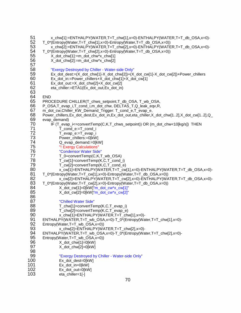
70

x_chw[1]:=ENTHALPY(WATER,T=T_chw[1],x=0)-ENTHALPY(WATER,T=T_db_OSA,x=0)-51 T_0*(Entropy(Water,T=T_chw[1],x=0)-Entropy(Water,T=T_db_OSA,x=0)) 52 x_chw[2]:=ENTHALPY(WATER,T=T_chw[2],x=0)-ENTHALPY(WATER,T=T_db_OSA,x=0)-53 T_0*(Entropy(Water,T=T_chw[2],x=0)-Entropy(Water,T=T_db_OSA,x=0)) 54 X_dot_chw[1]:=m_dot_chw*x_chw[1] 55 X_dot_chw[2]:=m_dot_chw*x_chw[2] 56 57 "Exergy Destroyed by Chiller - Water-side Only" 58 Ex_dot_dest:=(X_dot_chw[1]-X_dot_chw[2])+(X_dot_cw[1]-X_dot_cw[2])+Power_chillers 59 Ex_dot_in:=Power_chillers+X_dot_chw[1]+X_dot_cw[1] 60 Ex_dot_out:=X_dot_chw[2]+X_dot_cw[2] 61 eta_chiller:=ETA1(Ex_dot_out,Ex_dot_in) 62 63 END 64 PROCEDURE CHILLER(T_chws_setpoint,T_db_OSA, T_wb_OSA, 65 P_OSA,T_evap_i,T_cond_i,m_dot_chw, DELTAS_T,Q_leak_eqv,R, 66 m_dot_cw,Chiller_KW_Demand_Trigger: T_cond_e,T_evap_e, 67 Power_chillers,Ex_dot_dest,Ex_dot_in,Ex_dot_out,eta_chiller,X_dot_chw[1..2],X_dot_cw[1..2],Q_68 evap_demand) 69 IF (T_evap_i<=convertTemp(C,K,T_chws_setpoint)) OR (m_dot_chw<10[kg/s]) THEN 70 T_cond_e:=T_cond_i 71 T_evap_e:=T_evap_i 72 Power_chillers:=0[kW] 73 Q_evap_demand:=0[kW] 74 "! Exergy Calculations" 75 "Condensor Water Side" 76 T_0=convertTemp(C,K,T_wb_OSA) 77 T_cw[1]=convertTemp(K,C,T_cond_i) 78 T_cw[2]=convertTemp(K,C,T_cond_e) 79 x_cw[1]=ENTHALPY(WATER,T=T_cw[1],x=0)-ENTHALPY(WATER,T=T_db_OSA,x=0)-80 T_0*(Entropy(Water,T=T_cw[1],x=0)-Entropy(Water,T=T_db_OSA,x=0)) 81 x_cw[2]=ENTHALPY(WATER,T=T_cw[2],x=0)-ENTHALPY(WATER,T=T_db_OSA,x=0)-82 T_0*(Entropy(Water,T=T_cw[2],x=0)-Entropy(Water,T=T_db_OSA,x=0)) 83 X_dot_cw[1]=0[kW]"m_dot_cw*x_cw[1]" 84 X_dot_cw[2]=0[kW]"m_dot_cw*x_cw[2]" 85 86 "Chilled Water Side" 87 T_chw[1]=convertTemp(K,C,T_evap_i) 88 T_chw[2]=convertTemp(K,C,T_evap_e) 89 x_chw[1]=ENTHALPY(WATER,T=T_chw[1],x=0)-90 ENTHALPY(WATER,T=T_wb_OSA,x=0)-T_0*(Entropy(Water,T=T_chw[1],x=0)-91 Entropy(Water,T=T_wb_OSA,x=0)) 92 x_chw[2]=ENTHALPY(WATER,T=T_chw[2],x=0)-93 ENTHALPY(WATER,T=T_wb_OSA,x=0)-T_0*(Entropy(Water,T=T_chw[2],x=0)-94 Entropy(Water,T=T_wb_OSA,x=0)) 95 X_dot_chw[1]=0[kW] 96 X_dot_chw[2]=0[kW] 97 98 "Exergy Destroyed by Chiller - Water-side Only" 99 Ex_dot_dest=0[kW] 100 Ex_dot_in=0[kW] 101 Ex_dot_out=0[kW] 102 eta_chiller=1[-] 103

71

ELSE 104 CALL CHILLER2(T_chws_setpoint,T_db_OSA, T_wb_OSA, 105 P_OSA,T_evap_i,T_cond_i, m_dot_chw, DELTAS_T,Q_leak_eqv,R, 106 m_dot_cw,Chiller_KW_Demand_Trigger: T_cond_e,T_evap_e, 107 Power_chillers,Ex_dot_dest,Ex_dot_in,Ex_dot_out,eta_chiller,X_dot_chw[1..2],X_dot_cw[1..2],Q_108 evap_demand) 109 ENDIF 110 111 END 112 113 "! --------------------------END CHILLER FUNCTIONS--------------------------" 114 115 "! --------------------------BEGIN MAH FUNCTIONS--------------------------" 116 FUNCTION HUMIDIFY(omega_1, P1,T_db1,T_db_setpoint, T_db_setpoint_low, 117 T_db_setpoint_high, RH_setpoint, RH_setpoint_low, RH_setpoint_high) 118 “Calculates how much humidity is required for MAH” 119 omega|star=0[-] 120 omega_setpoint_min=HUMRAT(AIRH2O,T=T_db_setpoint_low,r= RH_setpoint_low,P=P1) 121 omega_setpoint_inter=HUMRAT(AIRH2O,T=T_db_setpoint_high,r= RH_setpoint_low,P=P1) 122 omega_setpoint_max=HUMRAT(AIRH2O,T=T_db_setpoint_high,r=RH_setpoint_high,P=P1) 123 T_wb_setpoint_min=WETBULB(AIRH2O,T=T_db_setpoint_low, r=RH_setpoint_low,P=P1) 124 T_wb_setpoint_inter=WETBULB(AIRH2O,T=T_db_setpoint_high, r=RH_setpoint_low,P=P1) 125 T_wb_setpoint_max=WETBULB(AIRH2O,T=T_db_setpoint_high,r=RH_setpoint_high,P=P1) 126 T_wb=WETBULB(AIRH2O,T=T_db1,w=omega_1,P=P1) 127 128 "Only humidify if W_osa is below minimum." 129 IF (omega_1<=omega_setpoint_min) THEN 130 IF(T_wb<=T_wb_setpoint_inter) THEN 131 omega_2=HUMRAT(AIRH2O,B=T_wb,r= RH_setpoint_low,P=P1) 132 ELSE 133 IF(T_wb<=T_wb_setpoint_max) THEN 134 omega_2=HUMRAT(AIRH2O,T=T_db_setpoint_high,B=T_wb,P=P1) 135 ELSE 136 IF(T_wb>T_wb_setpoint_max) THEN 137 omega_2=omega_setpoint_min 138 ENDIF 139 ENDIF 140 ENDIF 141 ELSE 142 omega_2=0[-] 143 ENDIF 144 omega|star=omega_2-omega_1 145 "Error Cache" 146 IF(omega|star<0) THEN 147 omega|star=0 148 ENDIF 149 150 HUMIDIFY:=omega|star 151 END 152 153 FUNCTION DEHUMIDIFY(omega_1,P1,T_db, T_db_setpoint, T_db_setpoint_low, 154 T_db_setpoint_high, RH_setpoint, RH_setpoint_low, RH_setpoint_high) 155 Calculates how much dehumidification is required for MAH 156

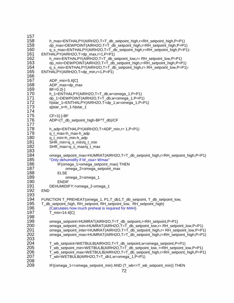
72

157 h_max=ENTHALPY(AIRH2O,T=T_db_setpoint_high,r=RH_setpoint_high,P=P1) 158 dp_max=DEWPOINT(AIRH2O,T=T_db_setpoint_high,r=RH_setpoint_high,P=P1) 159 q_s_max=ENTHALPY(AIRH2O,T=T_db_setpoint_high,r=RH_setpoint_high,P=P1)-160 ENTHALPY(AIRH2O,T=dp_max,r=1,P=P1) 161 h_min=ENTHALPY(AIRH2O,T=T_db_setpoint_low,r= RH_setpoint_low,P=P1) 162 dp_min=DEWPOINT(AIRH2O,T=T_db_setpoint_high,r=RH_setpoint_high,P=P1) 163 q_s_min=ENTHALPY(AIRH2O,T=T_db_setpoint_high,r= RH_setpoint_low,P=P1)-164 ENTHALPY(AIRH2O,T=dp_min,r=1,P=P1) 165 166 ADP_min=5.6[C] 167 ADP_max=dp_max 168 BF=0.2[-] 169 h_1=ENTHALPY(AIRH2O,T=T_db,w=omega_1,P=P1) 170 dp_1=DEWPOINT(AIRH2O,T=T_db,w=omega_1,P=P1) 171 h|star_1=ENTHALPY(AIRH2O,T=dp_1,w=omega_1,P=P1) 172 q|star_s=h_1-h|star_1 173 174 CF=1[-]-BF 175 ADP=(T_db_setpoint_high-BF*T_db)/CF 176 177 h_adp=ENTHALPY(AIRH2O,T=ADP_min,r= 1,P=P1) 178 q_t_max=h_max-h_adp 179 q_t_min=h_min-h_adp 180 SHR_min=q_s_min/q_t_min 181 SHR_max=q_s_max/q_t_max 182 183 omega_setpoint_max=HUMRAT(AIRH2O,T=T_db_setpoint_high,r=RH_setpoint_high,P=P1) 184 "Only dehumidify if W_osa> Wmax" 185 IF(omega_1>omega_setpoint_max) THEN 186 omega_2=omega_setpoint_max 187 ELSE 188 omega_2=omega_1 189 ENDIF 190 DEHUMIDIFY:=omega_2-omega_1 191 END 192 193 FUNCTION T_PREHEAT(omega_1, P1,T_db1,T_db_setpoint, T_db_setpoint_low, 194 T_db_setpoint_high, RH_setpoint, RH_setpoint_low, RH_setpoint_high) 195 Calculates how much preheat is required for MAH 196 T_min=14.4[C] 197 198 omega_setpoint=HUMRAT(AIRH2O,T=T_db_setpoint,r=RH_setpoint,P=P1) 199 omega_setpoint_min=HUMRAT(AIRH2O,T=T_db_setpoint_low,r= RH_setpoint_low,P=P1) 200 omega_setpoint_inter=HUMRAT(AIRH2O,T=T_db_setpoint_high,r= RH_setpoint_low,P=P1) 201 omega_setpoint_max=HUMRAT(AIRH2O,T=T_db_setpoint_high,r=RH_setpoint_high,P=P1) 202 203 T_wb_setpoint=WETBULB(AIRH2O,T=T_db_setpoint,w=omega_setpoint,P=P1) 204 T_wb_setpoint_min=WETBULB(AIRH2O,T=T_db_setpoint_low, r=RH_setpoint_low,P=P1) 205 T_wb_setpoint_max=WETBULB(AIRH2O,T=T_db_setpoint_high,r=RH_setpoint_high,P=P1) 206 T_wb=WETBULB(AIRH2O,T=T_db1,w=omega_1,P=P1) 207 208 IF((omega_1<=omega_setpoint_min) AND (T_wb<=T_wb_setpoint_min)) THEN 209

73

T_db|star=TEMPERATURE(AIRH2O,B=T_wb_setpoint_min,w=omega_1,P=P1) 210 ELSE 211 IF((omega_1<=omega_setpoint_max) AND (T_db1<=T_min)) THEN 212 T_db|star=T_min 213 ELSE 214 T_db|star=T_db1 "no preheat" 215 ENDIF 216 ENDIF 217 T_PREHEAT:=T_db|star 218 END 219 220 FUNCTION T_COOL(omega_1, P1, T_db1, T_db_setpoint, T_db_setpoint_low, 221 T_db_setpoint_high, RH_setpoint, RH_setpoint_low, RH_setpoint_high) 222 Calculates how much cooling is required for MAH 223 224 omega_setpoint=HUMRAT(AIRH2O,T=T_db_setpoint,r=RH_setpoint,P=P1) 225 omega_setpoint_min=HUMRAT(AIRH2O,T=T_db_setpoint_low,r= RH_setpoint_low,P=P1) 226 omega_setpoint_inter=HUMRAT(AIRH2O,T=T_db_setpoint_high,r= RH_setpoint_low,P=P1) 227 omega_setpoint_max=HUMRAT(AIRH2O,T=T_db_setpoint_high,r=RH_setpoint_high,P=P1) 228 229 T_wb_setpoint=WETBULB(AIRH2O,T=T_db_setpoint,w=omega_setpoint,P=P1) 230 T_wb_setpoint_min=WETBULB(AIRH2O,T=T_db_setpoint_low, r=RH_setpoint_low,P=P1) 231 T_wb_setpoint_inter=WETBULB(AIRH2O,T=T_db_setpoint_high, r=RH_setpoint_low,P=P1) 232 233 T_wb_setpoint_max=WETBULB(AIRH2O,T=T_db_setpoint_high,r=RH_setpoint_high,P=P1) 234 235 T_dp_max=DEWPOINT(AIRH2O,T=T_db_setpoint_high,r=RH_setpoint_high,P=P1) 236 omega_setpoint_inter=HUMRAT(AIRH2O,T=T_db_setpoint_high,r= RH_setpoint_low,P=P1) 237 238 239 ADP_min=5.6[C] 240 ADP_max=T_dp_max 241 BF=0.2[-] 242 243 CF=1[-]-BF 244 ADP=(T_db_setpoint_high-BF*T_db1)/CF 245 246 "W < Wmax, Then process is SHR=1" 247 IF(omega_1<=omega_setpoint_max) THEN 248 IF((omega_1>=omega_setpoint_inter) AND (T_db1 >=T_db_setpoint_high)) THEN 249 250 T_db|star=T_db_setpoint_high 251 ELSE 252 T|star=TEMPERATURE(AIRH2O,w=omega_1,r= RH_setpoint_low,P=P1) 253 IF((omega_1>=omega_setpoint_min) AND (T_db1 >=T|star)) THEN 254 T_db|star=T|star 255 ELSE 256 T_db|star=T_db1 257 ENDIF 258 ENDIF 259 ELSE 260 IF(omega_1>omega_setpoint_max) THEN 261 T_db|star=T_dp_max 262

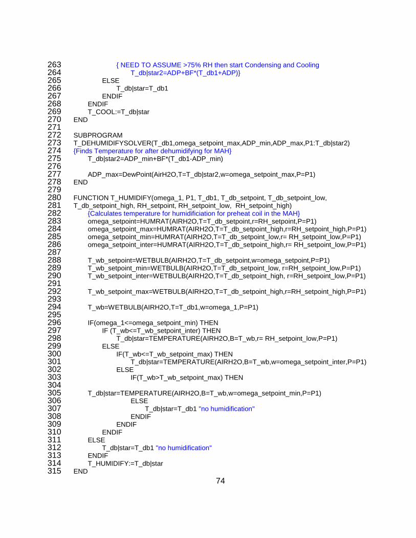
74

NEED TO ASSUME >75% RH then start Condensing and Cooling 263 T_db|star2=ADP+BF*(T_db1+ADP) 264 ELSE 265 T_db|star=T_db1 266 ENDIF 267 ENDIF 268 T_COOL:=T_db|star 269 END 270 271 SUBPROGRAM 272 T_DEHUMIDIFYSOLVER(T_db1,omega_setpoint_max,ADP_min,ADP_max,P1:T_db|star2) 273 Finds Temperature for after dehumidifying for MAH 274 T_db|star2=ADP_min+BF*(T_db1-ADP_min) 275 276 ADP_max=DewPoint(AirH2O,T=T_db|star2,w=omega_setpoint_max,P=P1) 277 END 278 279 FUNCTION T_HUMIDIFY(omega_1, P1, T_db1, T_db_setpoint, T_db_setpoint_low, 280 T_db_setpoint_high, RH_setpoint, RH_setpoint_low, RH_setpoint_high) 281 Calculates temperature for humidificiation for preheat coil in the MAH 282 omega_setpoint=HUMRAT(AIRH2O,T=T_db_setpoint,r=RH_setpoint,P=P1) 283 omega_setpoint_max=HUMRAT(AIRH2O,T=T_db_setpoint_high,r=RH_setpoint_high,P=P1) 284 omega_setpoint_min=HUMRAT(AIRH2O,T=T_db_setpoint_low,r= RH_setpoint_low,P=P1) 285 omega_setpoint_inter=HUMRAT(AIRH2O,T=T_db_setpoint_high,r= RH_setpoint_low,P=P1) 286 287 T_wb_setpoint=WETBULB(AIRH2O,T=T_db_setpoint,w=omega_setpoint,P=P1) 288 T_wb_setpoint_min=WETBULB(AIRH2O,T=T_db_setpoint_low, r=RH_setpoint_low,P=P1) 289 T_wb_setpoint_inter=WETBULB(AIRH2O,T=T_db_setpoint_high, r=RH_setpoint_low,P=P1) 290 291 T_wb_setpoint_max=WETBULB(AIRH2O,T=T_db_setpoint_high,r=RH_setpoint_high,P=P1) 292 293 T_wb=WETBULB(AIRH2O,T=T_db1,w=omega_1,P=P1) 294 295 IF(omega_1<=omega_setpoint_min) THEN 296 IF (T_wb<=T_wb_setpoint_inter) THEN 297 T_db|star=TEMPERATURE(AIRH2O,B=T_wb,r= RH_setpoint_low,P=P1) 298 ELSE 299 IF(T_wb<=T_wb_setpoint_max) THEN 300 T_db|star=TEMPERATURE(AIRH2O,B=T_wb,w=omega_setpoint_inter,P=P1) 301 ELSE 302 IF(T_wb>T_wb_setpoint_max) THEN 303 304 T_db|star=TEMPERATURE(AIRH2O,B=T_wb,w=omega_setpoint_min,P=P1) 305 ELSE 306 T_db|star=T_db1 "no humidification" 307 ENDIF 308 ENDIF 309 ENDIF 310 ELSE 311 T_db|star=T_db1 "no humidification" 312 ENDIF 313 T_HUMIDIFY:=T_db|star 314 END 315

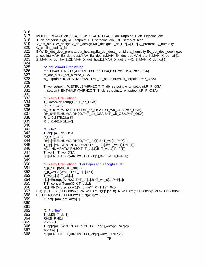
75

316 MODULE MAH(T_db_OSA, T_wb_OSA, P_OSA, T_db_setpoint, T_db_setpoint_low, 317 T_db_setpoint_high, RH_setpoint, RH_setpoint_low, RH_setpoint_high, 318 V_dot_air,BkW_design,V_dot_design,ME_design: T_db[1..7],w[1..7],Q_preheat, Q_humidify, 319 Q_cooling_coil,Q_fan, 320 BkW,Ex_dot_dest_preheat,eta_heating,Ex_dot_dest_humid,eta_humidify,Ex_dot_dest_cooling,et321 a_cooling,MAH_Ex_dot_dest,MAH_Ex_dot_in,MAH_Ex_dot_out,MAH_eta_II,MAH_X_dot_air[1..322 2],MAH_X_dot_hw[1..2], MAH_X_dot_huw[1],MAH_X_dot_chw[1..2],MAH_X_dot_cd[1]) 323 324 "V_dot_air=4000[ft^3/min]" 325 rho_OSA=DENSITY(AIRH2O,T=T_db_OSA,B=T_wb_OSA,P=P_OSA) 326 m_dot_air=V_dot_air*rho_OSA 327 w_setpoint=HUMRAT(AIRH2O,T=T_db_setpoint,r=RH_setpoint,P=P_OSA) 328 329 T_wb_setpoint=WETBULB(AIRH2O,T=T_db_setpoint,w=w_setpoint,P=P_OSA) 330 h_setpoint=ENTHALPY(AIRH2O,T=T_db_setpoint,w=w_setpoint,P=P_OSA) 331 332 "! Exergy Calculation" 333 T_0=convertTemp(C,K,T_db_OSA) 334 P_0=P_OSA 335 w_0=HUMRAT(AIRH2O,T=T_db_OSA,B=T_wb_OSA,P=P_OSA) 336 RH_0=RELHUM(AIRH2O,T=T_db_OSA,B=T_wb_OSA,P=P_OSA) 337 R_a=0.287[kJ/kg-K] 338 R_v=0.461[kJ/kg-K] 339 340 "1. Inlet" 341 T_db[1]=T_db_OSA 342 P[1]=P_OSA 343 RH[1]=RELHUM(AIRH2O,T=T_db[1],B=T_wb[1],P=P[1]) 344 T_dp[1]=DEWPOINT(AIRH2O,T=T_db[1],B=T_wb[1],P=P[1]) 345 w[1]=HUMRAT(AIRH2O,T=T_db[1],B=T_wb[1],P=P[1]) 346 T_wb[1]=T_wb_OSA 347 h[1]=ENTHALPY(AIRH2O,T=T_db[1],B=T_wb[1],P=P[1]) 348 349 "! Exergy Calculation" "Per Bejan and Kanoglu et.al." 350 c_p_a=Cp(Air,T=T_db[1]) 351 c_p_w=Cp(Water,T=T_db[1],x=1) 352 T_wb_s[1]=T_wb[1] 353 s[1]=Entropy(AirH2O,T=T_db[1],B=T_wb_s[1],P=P[1]) 354 T[1]=convertTemp(C,K,T_db[1]) 355 x[1]=RND((c_p_a+w[1]*c_p_w)*T_0*(T[1]/T_0-1-356 LN(T[1]/T_0))+(1+1.608*w[1])*R_a*T_0*LN(P[1]/P_0)+R_a*T_0*((1+1.608*w[1])*LN((1+1.608*w_357 0)/(1+1.608*w[1]))+1.608*w[1]*LN(w[1]/w_0)),3) 358 X_dot[1]=m_dot_air*x[1] 359 360 361 "2. Prefilter" 362 T_db[2]=T_db[1] 363 RH[2]=RH[1] 364 P[2]=P[1] 365 T_dp[2]=DEWPOINT(AIRH2O,T=T_db[2],w=w[2],P=P[2]) 366 w[2]=w[1] 367 h[2]=ENTHALPY(AIRH2O,T=T_db[2],w=w[2],P=P[2]) 368

76

T_wb[2]=WETBULB(AIRH2O,T=T_db[2],w=w[2],P=P[2]) 369 370 "! Exergy Calculation" 371 T_wb_s[2]=T_wb[2] 372 s[2]=Entropy(AirH2O,T=T_db[2],B=T_wb_s[2],P=P[2]) 373 T[2]=convertTemp(C,K,T_db[2]) 374 x[2]=RND((c_p_a+w[2]*c_p_w)*T_0*(T[2]/T_0-1-375 LN(T[2]/T_0))+(1+1.608*w[2])*R_a*T_0*LN(P[2]/P_0)+R_a*T_0*((1+1.608*w[2])*LN((1+1.608*w_376 0)/(1+1.608*w[2]))+1.608*w[2]*LN(w[2]/w_0)),3) 377 X_dot[2]=m_dot_air*x[2] 378 379 "3. Preheat" 380 P[3]=P[2] 381 w[3]=w[2] 382 T_db[3]=T_PREHEAT(w[3],P[3],T_db[2],T_db_setpoint, T_db_setpoint_low, 383 T_db_setpoint_high, RH_setpoint, RH_setpoint_low, RH_setpoint_high) 384 h[3]=ENTHALPY(AIRH2O,T=T_db[3],w=w[3],P=P[3]) 385 RH[3]=RELHUM(AIRH2O,T=T_db[3],w=w[3],P=P[3]) 386 T_dp[3]=DEWPOINT(AIRH2O,T=T_db[3],w=w[3],P=P[3]) 387 T_wb[3]=WETBULB(AIRH2O,T=T_db[3],w=w[3],P=P[3]) 388 Q_preheat=m_dot_air*(h[3]-h[2]) 389 390 "Determine flow rate for Hot water assuming 20F difference between supply and return" 391 "This should be enhanced using NTU or LMTD method" 392 "Assumed T_wb_OSA as reference point" 393 T_hw[1]=convertTemp(F,C,180[F]) 394 T_hw[2]=convertTemp(F,C,180[F]-20[F]) 395 c_p_hw=Cp(Water,T=T_hw[1],x=0) 396 Q_preheat=m_dot_hw*c_p_hw*(T_hw[1]-T_hw[2]) 397 T_wb_0=convertTemp(C,K,T_wb_OSA) 398 399 x_hw[1]=ENTHALPY(WATER,T=T_hw[1],x=0)-ENTHALPY(WATER,T=T_db_OSA,x=0)-400 T_0*(Entropy(Water,T=T_hw[1],x=0)-Entropy(Water,T=T_db_OSA,x=0)) 401 x_hw[2]=ENTHALPY(WATER,T=T_hw[2],x=0)-ENTHALPY(WATER,T=T_db_OSA,x=0)-402 T_0*(Entropy(Water,T=T_hw[2],x=0)-Entropy(Water,T=T_db_OSA,x=0)) 403 404 X_dot_hw[1]=m_dot_hw*x_hw[1] 405 X_dot_hw[2]=m_dot_hw*x_hw[2] 406 407 "! Exergy Calculation" 408 T_wb_s[3]=T_wb[3] 409 s[3]=Entropy(AirH2O,T=T_db[3],B=T_wb_s[3],P=P[3]) 410 T[3]=convertTemp(C,K,T_db[3]) 411 x[3]=RND((c_p_a+w[3]*c_p_w)*T_0*(T[3]/T_0-1-412 LN(T[3]/T_0))+(1+1.608*w[3])*R_a*T_0*LN(P[3]/P_0)+R_a*T_0*((1+1.608*w[3])*LN((1+1.608*w_413 0)/(1+1.608*w[3]))+1.608*w[3]*LN(w[3]/w_0)),3) 414 X_dot[3]=m_dot_air*x[3] 415 416 "Exergy Destroyed by Preheating Air - Sensible Only" 417 Ex_dot_dest_preheat=RND(X_dot[2]+X_dot_hw[1]-X_dot[3]-X_dot_hw[2],3) 418 Ex_dot_out_preheat=RND(X_dot[3]+X_dot_hw[2],3) 419 Ex_dot_in_preheat=RND(X_dot[2]+X_dot_hw[1],3) 420 eta_heating=ETA1(Ex_dot_out_preheat,Ex_dot_in_preheat) 421

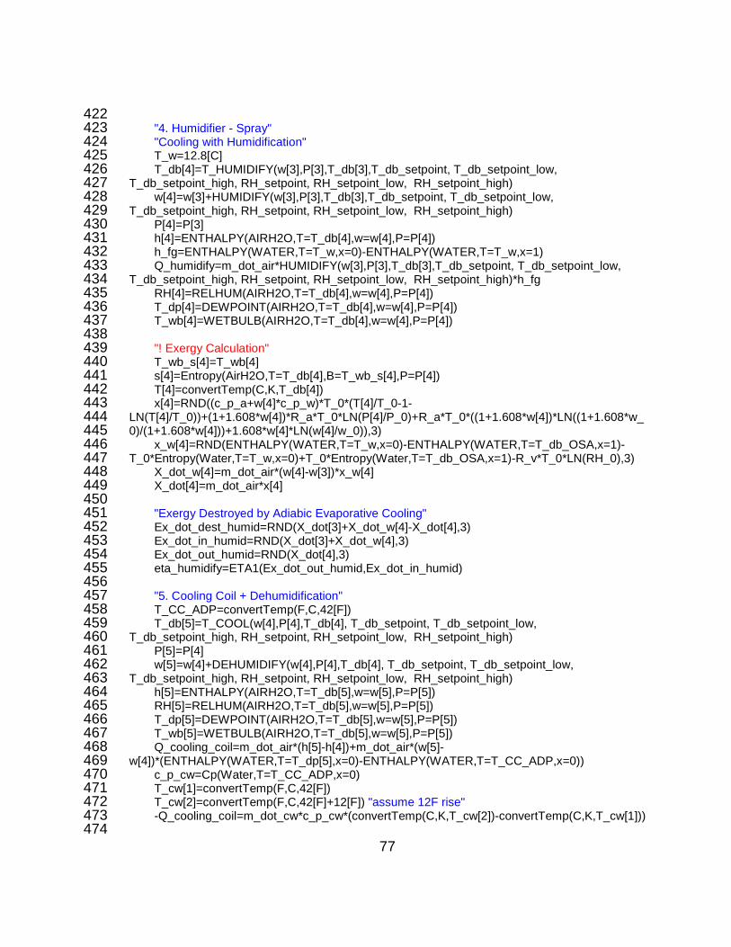
77

422 "4. Humidifier - Spray" 423 "Cooling with Humidification" 424 T_w=12.8[C] 425 T_db[4]=T_HUMIDIFY(w[3],P[3],T_db[3],T_db_setpoint, T_db_setpoint_low, 426 T_db_setpoint_high, RH_setpoint, RH_setpoint_low, RH_setpoint_high) 427 w[4]=w[3]+HUMIDIFY(w[3],P[3],T_db[3],T_db_setpoint, T_db_setpoint_low, 428 T_db_setpoint_high, RH_setpoint, RH_setpoint_low, RH_setpoint_high) 429 P[4]=P[3] 430 h[4]=ENTHALPY(AIRH2O,T=T_db[4],w=w[4],P=P[4]) 431 h_fg=ENTHALPY(WATER,T=T_w,x=0)-ENTHALPY(WATER,T=T_w,x=1) 432 Q_humidify=m_dot_air*HUMIDIFY(w[3],P[3],T_db[3],T_db_setpoint, T_db_setpoint_low, 433 T_db_setpoint_high, RH_setpoint, RH_setpoint_low, RH_setpoint_high)*h_fg 434 RH[4]=RELHUM(AIRH2O,T=T_db[4],w=w[4],P=P[4]) 435 T_dp[4]=DEWPOINT(AIRH2O,T=T_db[4],w=w[4],P=P[4]) 436 T_wb[4]=WETBULB(AIRH2O,T=T_db[4],w=w[4],P=P[4]) 437 438 "! Exergy Calculation" 439 T_wb_s[4]=T_wb[4] 440 s[4]=Entropy(AirH2O,T=T_db[4],B=T_wb_s[4],P=P[4]) 441 T[4]=convertTemp(C,K,T_db[4]) 442 x[4]=RND((c_p_a+w[4]*c_p_w)*T_0*(T[4]/T_0-1-443 LN(T[4]/T_0))+(1+1.608*w[4])*R_a*T_0*LN(P[4]/P_0)+R_a*T_0*((1+1.608*w[4])*LN((1+1.608*w_444 0)/(1+1.608*w[4]))+1.608*w[4]*LN(w[4]/w_0)),3) 445 x_w[4]=RND(ENTHALPY(WATER,T=T_w,x=0)-ENTHALPY(WATER,T=T_db_OSA,x=1)-446 T_0*Entropy(Water,T=T_w,x=0)+T_0*Entropy(Water,T=T_db_OSA,x=1)-R_v*T_0*LN(RH_0),3) 447 X_dot_w[4]=m_dot_air*(w[4]-w[3])*x_w[4] 448 X_dot[4]=m_dot_air*x[4] 449 450 "Exergy Destroyed by Adiabic Evaporative Cooling" 451 Ex_dot_dest_humid=RND(X_dot[3]+X_dot_w[4]-X_dot[4],3) 452 Ex_dot_in_humid=RND(X_dot[3]+X_dot_w[4],3) 453 Ex_dot_out_humid=RND(X_dot[4],3) 454 eta_humidify=ETA1(Ex_dot_out_humid,Ex_dot_in_humid) 455 456 "5. Cooling Coil + Dehumidification" 457 T_CC_ADP=convertTemp(F,C,42[F]) 458 T_db[5]=T_COOL(w[4],P[4],T_db[4], T_db_setpoint, T_db_setpoint_low, 459 T_db_setpoint_high, RH_setpoint, RH_setpoint_low, RH_setpoint_high) 460 P[5]=P[4] 461 w[5]=w[4]+DEHUMIDIFY(w[4],P[4],T_db[4], T_db_setpoint, T_db_setpoint_low, 462 T_db_setpoint_high, RH_setpoint, RH_setpoint_low, RH_setpoint_high) 463 h[5]=ENTHALPY(AIRH2O,T=T_db[5],w=w[5],P=P[5]) 464 RH[5]=RELHUM(AIRH2O,T=T_db[5],w=w[5],P=P[5]) 465 T_dp[5]=DEWPOINT(AIRH2O,T=T_db[5],w=w[5],P=P[5]) 466 T_wb[5]=WETBULB(AIRH2O,T=T_db[5],w=w[5],P=P[5]) 467 Q_cooling_coil=m_dot_air*(h[5]-h[4])+m_dot_air*(w[5]-468 w[4])*(ENTHALPY(WATER,T=T_dp[5],x=0)-ENTHALPY(WATER,T=T_CC_ADP,x=0)) 469 c_p_cw=Cp(Water,T=T_CC_ADP,x=0) 470 T_cw[1]=convertTemp(F,C,42[F]) 471 T_cw[2]=convertTemp(F,C,42[F]+12[F]) "assume 12F rise" 472 -Q_cooling_coil=m_dot_cw*c_p_cw*(convertTemp(C,K,T_cw[2])-convertTemp(C,K,T_cw[1])) 473 474

78

"! Exergy Calculation" 475 T_wb_s[5]=T_wb[5] 476 s[5]=Entropy(AirH2O,T=T_db[5],B=T_wb_s[5],P=P[5]) 477 T[5]=convertTemp(C,K,T_db[5]) 478 x[5]=RND((c_p_a+w[5]*c_p_w)*T_0*(T[5]/T_0-1-479 LN(T[5]/T_0))+(1+1.608*w[5])*R_a*T_0*LN(P[5]/P_0)+R_a*T_0*((1+1.608*w[5])*LN((1+1.608*w_480 0)/(1+1.608*w[5]))+1.608*w[5]*LN(w[5]/w_0)),3) 481 X_dot[5]=m_dot_air*x[5] 482 483 x_cw[1]=ENTHALPY(WATER,T=T_cw[1],x=0)-ENTHALPY(WATER,T=T_db_OSA,x=0)-484 T_0*(Entropy(Water,T=T_cw[1],x=0)-Entropy(Water,T=T_db_OSA,x=0)) 485 x_cw[2]=ENTHALPY(WATER,T=T_cw[2],x=0)-ENTHALPY(WATER,T=T_db_OSA,x=0)-486 T_0*(Entropy(Water,T=T_cw[2],x=0)-Entropy(Water,T=T_db_OSA,x=0)) 487 488 X_dot_cw[1]=RND(m_dot_cw,3)*x_cw[1] 489 X_dot_cw[2]=RND(m_dot_cw,3)*x_cw[2] 490 491 x_w[5]=ENTHALPY(WATER,T=T_CC_ADP,x=0)-ENTHALPY(WATER,T=T_db_OSA,x=1)-492 T_0*Entropy(Water,T=T_CC_ADP,x=0)+T_0*Entropy(Water,T=T_db_OSA,x=1)-493 R_v*T_0*LN(RH_0) 494 495 X_dot_w[5]=RND(m_dot_air*(w[5]-w[4])*x_w[5],3) 496 497 "Exergy Destroyed by Cooling Air" 498 Ex_dot_dest_cooling=RND(X_dot[4]+X_dot_cw[1]-X_dot_cw[2]-X_dot[5]-X_dot_w[5],3) 499 Ex_dot_in_cooling=RND(X_dot[4]+X_dot_cw[1],3) 500 Ex_dot_out_cooling=RND(X_dot_cw[2]+X_dot[5]+X_dot_w[5],3) 501 eta_cooling=ETA2(Ex_dot_out_cooling,Ex_dot_in_cooling) 502 503 "6. Fan" 504 V_dot_air[6]=m_dot_air/Density(AirH2O,T=T_db[5],w=w[5],P=P[5]) 505 "BkW_design=7.5[hp]*convert(hp,kW)""!LINK TO MAH SETTINGS" 506 "V_dot_design=4000[cfm]*convert(cfm,m^3/s)""!LINK TO MAH SETTINGS" 507 "ME_design=0.93[-]""!LINK TO MAH SETTINGS" 508 AkW=ME_design*BkW_design*(V_dot_air[6]/V_dot_design)^3"!LINK TO MAH SETTINGS" 509 BkW=BkW_design*(V_dot_air[6]/V_dot_design)^3"!LINK TO MAH SETTINGS" 510 DELTAT_FkW=(BkW-AkW)/(m_dot_air*c_p_a)"!LINK TO MAH SETTINGS" 511 512 T_db[6]=convertTemp(K,C,convertTemp(C,K,T_db[5])+DELTAT_FkW) 513 w[6]=w[5] 514 P[6]=P[5] 515 516 RH[6]=RELHUM(AIRH2O,T=T_db[6],w=w[6],P=P[6]) 517 h[6]=ENTHALPY(AIRH2O,T=T_db[6],w=w[6],P=P[6]) 518 Q_fan=m_dot_air*(h[6]-h[5]) 519 T_dp[6]=DEWPOINT(AIRH2O,T=T_db[6],w=w[6],P=P[6]) 520 T_wb[6]=WETBULB(AIRH2O,T=T_db[6],w=w[6],P=P[6]) 521 522 "! Exergy Calculation" 523 T_wb_s[6]=T_wb[6]-.0001[C]"offset T_wb by -.01C because EES can not solve when 524 Tdb=Twb for entrophy" 525 s[6]=Entropy(AirH2O,T=T_db[6],B=T_wb_s[6],P=P[6]) 526 T[6]=convertTemp(C,K,T_db[6]) 527

79

x[6]=(c_p_a+w[6]*c_p_w)*T_0*(T[6]/T_0-1-528 LN(T[6]/T_0))+(1+1.608*w[6])*R_a*T_0*LN(P[6]/P_0)+R_a*T_0*((1+1.608*w[6])*LN((1+1.608*w_529 0)/(1+1.608*w[6]))+1.608*w[6]*LN(w[6]/w_0)) 530 X_dot[6]=m_dot_air*x[6] 531 "Exergy Destroyed by Cooling Air " 532 Ex_dot_dest_fan=RND(X_dot[6]-X_dot[5],3) 533 Ex_dot_in_fan=RND(X_dot[5]+BkW,3) 534 Ex_dot_out_fan=RND(X_dot[6]+X_dot_w[5],3) 535 eta_fan=ETA1(Ex_dot_out_fan,Ex_dot_in_fan) 536 537 "7. Final Filter" 538 T_db[7]=T_db[6] 539 P[7]=P[6] 540 w[7]=w[6] 541 T_dp[7]=DEWPOINT(AIRH2O,T=T_db[7],w=w[7],P=P[7]) 542 RH[7]=RELHUM(AIRH2O,T=T_db[7],w=w[7],P=P[7]) 543 h[7]=ENTHALPY(AIRH2O,T=T_db[7],w=w[7],P=P[7]) 544 T_wb[7]=WETBULB(AIRH2O,T=T_db[7],w=w[7],P=P[7]) 545 546 MAH_Ex_dot_dest=Ex_dot_dest_fan+Ex_dot_dest_cooling+Ex_dot_dest_humid+Ex_dot_de547 st_preheat+BkW 548 MAH_Ex_dot_in=X_dot[1]+X_dot_hw[1]+X_dot_w[4]+X_dot_cw[1]+BkW 549 MAH_Ex_dot_out=X_dot[6]+X_dot_hw[2]+X_dot_cw[2]+X_dot_w[5] 550 MAH_eta_II=ETA1(MAH_Ex_dot_out,MAH_Ex_dot_in) 551 MAH_X_dot_air[1..2]=[X_dot[1],X_dot[6]] 552 MAH_X_dot_hw[1..2]=[X_dot_hw[1],X_dot_hw[2]] 553 MAH_X_dot_huw[1]=X_dot_w[4] 554 MAH_X_dot_chw[1..2]=[X_dot_cw[1],X_dot_cw[2]] 555 MAH_X_dot_cd[1]=X_dot_w[5] 556 557 END 558 "! --------------------------END MAH FUNCTIONS--------------------------" 559 "! --------------------------BEGIN CRAH FUNCTIONS--------------------------" 560 561 MODULE CRAH(T_db_OSA, T_wb_OSA, 562 P_OSA,Airflow,omega_RA,T_RA,T_SA,T_chws,P_RA,P_chw,DELTAT_CHW,CRAH_Qty,CRAH563 _AirFLow,CRAH_BkW:m_dot_chws,T_chwr,Total_BkW,Ex_dot_dest_cooling,Ex_dot_in_cooling,564 Ex_dot_out_cooling,eta_cooling,CRAH_X_dot_air[1..2],CRAH_X_dot_chw[1..2]) 565 566 Things to do 567 1) Convert logic for precision conditioning, 568 2) Add bypass flow around coil 569 3) Add ESP (~0.3 in WC) and SP (0.5 in WC) calcs to estimate BHP 570 4) Add Pressure drop accross filter - 30% ASHRAE 571 5) Add Humidification 572 573 "! Exergy Calculation" 574 T_0=convertTemp(C,K,T_db_OSA) 575 P_0=P_OSA 576 w_0=HUMRAT(AIRH2O,T=T_db_OSA,B=T_wb_OSA,P=P_OSA) 577 RH_0=RELHUM(AIRH2O,T=T_db_OSA,B=T_wb_OSA,P=P_OSA) 578 R_a=0.287[kJ/kg-K] 579 R_v=0.461[kJ/kg-K] 580

80

581 "Air Side Properties - State 1" 582 T_db[1]=T_RA 583 w[1]=omega_RA 584 P[1]=P_RA 585 RH[1]=RELHUM(AIRH2O,T=T_db[1],w=w[1],P=P[1]) 586 T_dp[1]=DEWPOINT(AIRH2O,T=T_db[1],w=w[1],P=P[1]) 587 h[1]=ENTHALPY(AIRH2O,T=T_db[1],w=w[1],P=P[1]) 588 rho_ra[1]=Density(AirH2O,T=T_db[1],w=w[1],P=P[1]) 589 FlowRate_ra=Airflow 590 m_dot_air=FlowRate_ra*rho_ra[1] 591 Q[1]=m_dot_air*h[1] 592 593 "! Exergy Calculation" "Per Bejan and Kanoglu et.al." 594 c_p_a=Cp(Air,T=T_db[1]) 595 c_p_w=Cp(Water,T=T_db[1],x=1) 596 s[1]=Entropy(AirH2O,T=T_db[1],w=w[1],P=P[1]) 597 T[1]=convertTemp(C,K,T_db[1]) 598 x[1]=RND((c_p_a+w[1]*c_p_w)*T_0*(T[1]/T_0-1-599 LN(T[1]/T_0))+(1+1.608*w[1])*R_a*T_0*LN(P[1]/P_0)+R_a*T_0*((1+1.608*w[1])*LN((1+1.608*w_600 0)/(1+1.608*w[1]))+1.608*w[1]*LN(w[1]/w_0)),3) 601 X_dot[1]=m_dot_air*x[1] 602 603 "State 2" 604 P[2]=P[1] 605 T_db[2]=T_SA-DELTAT_motor 606 w[2]=w[1] "Assume no dehumidification" 607 h[2]=Enthalpy(AirH2O,T=T_db[2],w=w[2],P=P[2]) 608 Q[2]=m_dot_air*h[2] 609 Q_coil=Q[1]-Q[2]-Q_m 610 611 "! Exergy Calculation" "Per Bejan and Kanoglu et.al." 612 s[2]=Entropy(AirH2O,T=T_db[2],w=w[2],P=P[2]) 613 T[2]=convertTemp(C,K,T_db[2]) 614 x[2]=RND((c_p_a+w[2]*c_p_w)*T_0*(T[2]/T_0-1-615 LN(T[2]/T_0))+(1+1.608*w[2])*R_a*T_0*LN(P[2]/P_0)+R_a*T_0*((1+1.608*w[2])*LN((1+1.608*w_616 0)/(1+1.608*w[2]))+1.608*w[2]*LN(w[2]/w_0)),3) 617 X_dot[2]=m_dot_air*x[2] 618 619 "Motor Heat" 620 BkW_per_CRAH=CRAH_BkW*((FlowRate_ra/CRAH_Qty)/(CRAH_AirFLow*convert(L/s,m^3621 /s)))^3 622 ME=0.72[-] 623 AkW=ME*BkW_per_CRAH 624 FkW=BkW_per_CRAH*(1-ME) 625 Q_m=FkW*CRAH_Qty 626 Total_BkW=CRAH_Qty*BkW_per_CRAH 627 DELTAT_motor=BkW_per_CRAH*(1-ME)/(c_p_a*m_dot_air/CRAH_Qty) 628 "Q_T=Q_coil+Q_m" 629 630 "Chilled Water Flow" 631 P_chw[1]=P_chw 632 "P_chw[2]=P_chw[1]+DELTAP_chw" 633

81

T_chwr=T_chws+DELTAT_CHW 634 cp_chw=Cp(Water,T=T_chws,x=0) 635 Q_coil=m_dot_chws*(Enthalpy(Water,T=T_chwr,x=0)-Enthalpy(Water,T=T_chws,x=0)) 636 637 "! Exergy Calculation" "Per Bejan and Kanoglu et.al." 638 T_cw[1]=T_chws 639 T_cw[2]=T_chwr 640 x_cw[1]=ENTHALPY(WATER,T=T_cw[1],x=0)-ENTHALPY(WATER,T=T_db_OSA,x=0)-641 T_0*(Entropy(Water,T=T_cw[1],x=0)-Entropy(Water,T=T_db_OSA,x=0)) 642 x_cw[2]=ENTHALPY(WATER,T=T_cw[2],x=0)-ENTHALPY(WATER,T=T_db_OSA,x=0)-643 T_0*(Entropy(Water,T=T_cw[2],x=0)-Entropy(Water,T=T_db_OSA,x=0)) 644 X_dot_cw[1]=m_dot_chws*x_cw[1] 645 X_dot_cw[2]=m_dot_chws*x_cw[2] 646 647 T_CC_ADP=T_cw[1] 648 x_w[3]=ENTHALPY(WATER,T=T_CC_ADP,x=0)-ENTHALPY(WATER,T=T_db_OSA,x=1)-649 T_0*Entropy(Water,T=T_CC_ADP,x=0)+T_0*Entropy(Water,T=T_db_OSA,x=1)-650 R_v*T_0*LN(RH_0) 651 X_dot_w[3]=RND(m_dot_air*(w[2]-w[1])*x_w[3],3) 652 653 CRAH_X_dot_air[1]=X_dot[1] 654 CRAH_X_dot_air[2]=X_dot[2] 655 CRAH_X_dot_chw[1]=X_dot_cw[1] 656 CRAH_X_dot_chw[2]=X_dot_cw[2] 657 "Exergy Destroyed by Cooling Air" 658 Ex_dot_dest_cooling=(X_dot[1]-X_dot[2])+(X_dot_cw[1]-X_dot_cw[2])+Total_BkW 659 Ex_dot_out_cooling=X_dot_cw[2]+X_dot[2]+X_dot_w[3] 660 Ex_dot_in_cooling=X_dot[1]+X_dot_cw[1]+Total_BkW 661 eta_cooling=ETA2(Ex_dot_dest_cooling,Ex_dot_in_cooling) 662 "rho_chw=Density(Water,T=T_chws,P=P_chw[1])" 663 "V_dot_chws=(m_dot_chws/rho_chw)*convert(ft^3/hr,gpm)" 664 665 "Curve Fitted Pressure drop as a function of GPM, based on FH600C" 666 "DELTAP_chw=0.0087*V_dot_chws^1.8386" 667 668 END 669 670 "! --------------------------END CRAH FUNCTIONS--------------------------" 671 672 "! --------------------------BEGIN WEATHER BIN FUNCTIONS--------------------------" 673 PROCEDURE WEATHERBINDATAMAXTEMP(P_OSA: T_db_OSA_max, 674 T_wb_OSA_max,RH_OSA_max, BinMonth$, BinDay,BinHourMax) 675 Retrieves selected data from lookup table and calculates RH 676 i:=0 677 NRows:=8760 678 T_db_OSA_max:=-999 679 T_wb_OSA_max:=-999 680 Repeat 681 i:=i+1 682 T_db_OSA=Lookup('WEATHER',i,'Dry Bulb') 683 IF(T_db_OSA>T_db_OSA_max) THEN 684 T_db_OSA_max:=T_db_OSA 685 T_wb_OSA_max:=Lookup('WEATHER',i,'Wet Bulb') 686

82

RH_OSA_max:=RelHum(AirH2O,T=T_db_OSA,B=T_wb_OSA_max,P=P_OSA) 687 BinMonth$:=Lookup$('WEATHER',i,'Month') 688 BinDay:=Lookup('WEATHER',i,'Day') 689 BinHourMax:=i 690 ENDIF 691 until (i>=NRows) 692 693 END 694 PROCEDURE WEATHERBINDATA(City$,BinHour, P_OSA: T_db_OSA, T_wb_OSA,RH_OSA, 695 BinMonth$, BinDay) 696 Retrieves selected data from lookup table and calculates RH 697 Data from Table is in ENG units. This program converts to SI 698 T_db_OSA:=convertTemp(F,C,Lookup(City$,BinHour,'Dry Bulb')) 699 T_wb_OSA:=convertTemp(F,C,Lookup(City$,BinHour,'Wet Bulb')) 700 IF (T_db_OSA<=T_wb_OSA) THEN "EES CANNOT SOLVE IF TWB>=TDB" 701 T_wb_OSA:=T_db_OSA-.0001[C] 702 ENDIF 703 RH_OSA:=RelHum(AirH2O,T=T_db_OSA,B=T_wb_OSA,P=P_OSA) 704 BinMonth$:=Lookup$(City$,BinHour,'Month') 705 BinDay:=Lookup(City$,BinHour,'Day') 706 END 707 FUNCTION GETALTITUDEDATA(City$) 708 Retrieves selected data from lookup table and returns altitude 709 i=0 710 N=15 711 Repeat 712 i:=i+1 713 CityName$=Lookup$('CITYLIST',i,'City') 714 IF (CityName$=City$) THEN 715 GETALTITUDEDATA:=Lookup('CITYLIST',i,'Altitude') 716 ENDIF 717 Until (i>=N) 718 END 719 FUNCTION BAROMETRICPRESSURE(ALTITUDE) 720 ASHRAE 2005 FUNDAMENTALS CHAPTER 6., equation 6.3 721 BAROMETRICPRESSURE:=14.696*(1-6.8754*10^(-6)*ALTITUDE)^(5.2559) 722 END 723 "! --------------------------END WEATHER BIN FUNCTIONS--------------------------" 724 725 "! --------------------------BEGIN COOLING LOAD CALCULATIONS-------------------------" 726 PROCEDURE DATACENTERLOAD(NRows, T_db_setpoint, P_OSA, RH_setpoint: Airflow, 727 HeatLoad,Racks) 728 729 Calculates and sets values for the DC equipment lookup table 730 Future: Add PDU Heat loads, Lighting, and people. 731 732 733 P=P_OSA 734 cp=Cp(AirH2O,T=T_db_setpoint,r=RH_setpoint,P=P) 735 rho=Density(AirH2O,T=T_db_setpoint,r=RH_setpoint,P=P) 736 737 i:=0 738 Airflow:=0 739

83

HeatLoad:=0 740 Racks:=0 741 repeat 742 i:=i+1 743 744 Power=Lookup('DC Equipment',i,'Cabinet Rating') 745 DeltaT=Lookup('DC Equipment',i,'Temperature Rise') 746 Qty=Lookup('DC Equipment',i,'Quantity') 747 748 Lookup('DC Equipment',i,'Airflow/Cabinet')=Power/(rho*cp*DeltaT) 749 Lookup('DC Equipment',i,'Total Airflow')=Power*Qty/(rho*cp*DeltaT) 750 Lookup('DC Equipment',i,'Total Power')=Power*Qty 751 Airflow:=Airflow+Power/(rho*cp*DeltaT)*Qty 752 HeatLoad:=HeatLoad+Power*Qty 753 Racks:=Racks+Qty 754 until (i>=NRows) 755 END 756 "! --------------------------END COOLING LOAD CALCULATIONS-------------------------" 757 "! --------------------------BEGIN EXERGY FUNCTIONS-------------------------" 758 FUNCTION FLOWEXERGY(T_o, T_wb_o, P_o,s,h) 759 omega_o=HumRat(AirH2O,T=T_o,B=T_wb_o,P=P_o) 760 h_o=ENTHALPY(AirH2O,T=T_o,B=T_wb_o,P=P_o) 761 s_o=Entropy(AirH2O,T=T_o,B=T_wb_o,P=P_o) 762 Flow Exergy 763 FLOWEXERGY:=(h-h_o)-ConvertTemp(F,R,T_o)*(s-s_o) 764 END 765 766 FUNCTION WATERFLOWEXERGY(T_o, T_wb_o, P_o,T) 767 h_o=ENTHALPY(Water,T=T_wb_o,P=P_o) 768 s_o=Entropy(Water,T=T_wb_o,P=P_o) 769 h=ENTHALPY(Water,T=T,x=0) 770 s=Entropy(Water,T=T,x=0) 771 Flow Exergy 772 WATERFLOWEXERGY:=(h-h_o)-ConvertTemp(F,R,T_o)*(s-s_o) 773 END 774 "! --------------------------END EXERGY FUNCTIONS-------------------------" 775 776 "! --------------------------BEGIN COOLING TOWER FUNCTIONS--------------------------" 777 778 "! --------------------------BEGIN COOLING TOWER FUNCTIONS--------------------------" 779 780 PROCEDURE 781 Muangnoi(L,T_db_i,T_wb_i,T_w_i,T_cw_setpoint,A,Ka,P1,Le,Z,N:G,T_db_e,T_wb_e,T_w_e,X_d782 es,X_w_i,X_w_e,X_air_i,X_air_e,Q_rejected,IW_makeup) 783 ! An exergy analysis on the performance of a counterflow wet cooling tower 784 T. Muangnoi et al. / Applied Thermal Engineering 27 (2007) 910-917 785 786 "Set Step Size to intgrate through Tower Hieght" 787 dZ=Z/(N-1[-]) 788 789 "Specific Heats" 790 cp_a=Cp(Air,T=T_db_i) "Dry Air" 791 cp_w=Cp(Water,T=T_w_i,x=0) "Water" 792

84

cp_v=Cp(Water,T=T_db_i,x=1) "Water Vapor" 793 T_w_inlet=T_w_i 794 T_db[1]=T_db_i 795 T_wb[1]=T_wb_i 796 w[1]=HumRat(AirH2O,T=T_db_i,B=T_wb_i,P=P1) 797 h[1]=Enthalpy(AirH2O,T=T_db_i,B=T_wb_i,P=P1) 798 rh[1]=RelHum(AirH2O,T=T_db_i,B=T_wb_i,P=P1) 799 rho[1]=Density(AirH2O,T=T_db_i,B=T_wb_i,P=P1) 800 801 "Convergence Criteria" 802 eta|star_L=5E-9[kg/s] 803 eta|star_G=5E-9[kg/s] 804 MaxIter=100 805 806 "Exergy Calculations" 807 "Restricted Dead State" 808 T_0=T_db_i 809 P_0=P1 810 rh_0=RelHum(AirH2O,T=T_db_i,B=T_wb_i,P=P_0) 811 w_0=HumRat(AirH2O,T=T_db_i,r=rh[1],P=P_0) 812 813 h_f_0=Enthalpy(Water,T=T_0,x=0) 814 s_f_0=Entropy(Water,T=T_0,x=0) 815 "Gas Constants" 816 R_v=0.4615[kJ/kg-K] "Water Vapor" 817 R_a=0.28703[kJ/kg-K] "Dry Air" 818 819 "Dead State" 820 "T_00=T_wb_i" 821 "rh_00=0.8[-]" 822 rh_00=rh_0 823 "w_00=HumRat(AirH2O,T=T_0,r=rh_00,P=P_0)" 824 w_00=w_0 825 "Initial Guess" 826 L[1]=L-.01[kg/s] 827 Z[1]=0 828 j=1 829 REPEAT 830 Z[j+1]=Z[j]+dZ 831 j=j+1 832 UNTIL (j>N) 833 834 T_cw_setpoint_new=T_cw_setpoint 835 "LG=2" 836 "Initital Guess at G" 837 G_max=A*rho[1]*1.75[m/s] 838 839 "REPEAT" 840 k=1 841 T_w[1]=T_cw_setpoint_new 842 Q_w=L*cp_w*(T_w_i-T_w[1]) 843 h[N]=Enthalpy(AirH2O,T=T_w_i,B=T_w_i,P=P1) 844 G=Q_w/(h[N]-h[1]) 845

85

IF G_guess>G_max THEN 846 G=G_max 847 ELSE 848 G=G_guess 849 ENDIF 850 REPEAT 851 852 i=1 853 854 REPEAT 855 856 j=1 857 858 REPEAT 859 860 "Saturated humidity ratio elevated at T_w" 861 w_s_w[j]=HumRat(AirH2O,T=T_w[j],B=T_w[j],P=P1) 862 "Saturated enthalpy of water vapor elevated at T_w" 863 h_g_w[j]=Enthalpy(Water,T=T_w[j],x=1) 864 865 "Equation 5: Change of Air Enthalpy" 866 dh[j]=(Ka*A)/G*(Le*cp_a*(T_w[j]-T_db[j])+h_g_w[j]*(w_s_w[j]-w[j]))*dZ 867 h[j+1]=h[j]+dh[j] 868 869 "Equation 6: Change of Humidity Ratio" 870 dw[j]=(Ka*A)/G*(w_s_w[j]-w[j])*dZ 871 w[j+1]=w[j]+dw[j] 872 873 "Equation 7: Change of Water Temperature" 874 h_f_w=Enthalpy(Water,T=T_w[j],x=0) 875 "cp_w=Cp(Water,T=T_w[j],x=0)" 876 dT_w[j]=G/(L[j]*cp_w)*(dh[j]-h_f_w*dw[j]) 877 T_w[j+1]=T_w[j]+dT_w[j] 878 879 T_db[j+1]=Temperature(AirH2O,h=h[j+1],w=w[j+1],P=P1) 880 T_wb[j+1]=WetBulb(AirH2O,T=T_db[j+1],w=w[j+1],P=P1) 881 882 T_wb[j+1]=WetBulb(AirH2O,h=h[j+1],w=w[j+1],P=P1) 883 T_db[j+1]=Temperature(AirH2O,B=T_wb[j+1],w=w[j+1],P=P1) 884 885 rh[j+1]=RelHum(AirH2O,T=T_db[j+1],B=T_wb[j+1],P=P1) 886 L[j+1]=L[j]+G*(w[j+1]-w[j]) 887 888 "Exergy Calculations" 889 T0=convertTemp(C,K,T_0) 890 891 "Water Side" 892 s_f_w[j]=Entropy(Water,T=T_w[j],x=0) 893 X_w[j]=L[j]*((h_f_w-h_f_0)-T0*(s_f_w[j]-s_f_0)-R_v*T0*ln(rh_00)) 894 895 "Air Side" 896 T=convertTemp(C,K,T_db[j]) 897 T0=convertTemp(C,K,T_0) 898

86

X_air[j]=G*((cp_a-w[j]*cp_v)*(T-T0-899 T0*ln(T/T0))+R_a*T0*((1+1.608*w[j])*ln((1+1.608*w_00)/(1+1.608*w[j]))+1.608*w[j]*ln(w[j]/w_00))900 ) 901 902 IF (T_w[j]>T_w_i) THEN 903 T_w[j]=T_w_i 904 ENDIF 905 906 j=j+1 907 908 UNTIL(j>N) 909 910 dL_error=L-L[N] 911 L[1]=L[1]+dL_error 912 i=i+1 913 914 UNTIL (abs(L[N]-L)<=eta|star_L) 915 916 T_error=T_w[N]-T_w_i 917 Q_error=L*cp_w*T_error 918 dh_error=h[1]-h[N] 919 dw_error=w[1]-w[N] 920 h_f_w=Enthalpy(Water,T=average(T_w[N],T_w[1]),x=0) 921 G_error=Q_error/(dh_error-h_f_w*dw_error) 922 "G_error=Q_error/dh_error" 923 924 G=G+G_error/2 925 926 IF G>G_Max THEN 927 G=G_Max 928 G_error=0 929 ENDIF 930 931 k=k+1 932 UNTIL ((ABS(G_error)<=eta|star_G) OR (k>MaxIter)) 933 Reset Leaving Water Temperature because Fan is Maxed out 934 935 "T_cw_setpoint_new=T_w[1]+0.1[C]" 936 IF (T_cw_setpoint_new+1.5)>T_w_i THEN 937 G=G_Max 938 T_w_i=T_w_inlet+2 939 T_cw_setpoint_new=T_cw_setpoint 940 ENDIF 941 "UNTIL (G<G_Max)" 942 943 X_w_i=X_w[N] 944 X_w_e=X_w[1] 945 X_air_i=X_air[1] 946 X_air_e=X_air[N] 947 X_des=((X_w_i-X_w_e)+(X_air_i-X_air_e)) 948 949 T_db_e=T_db[N] 950 T_wb_e=T_wb[N] 951

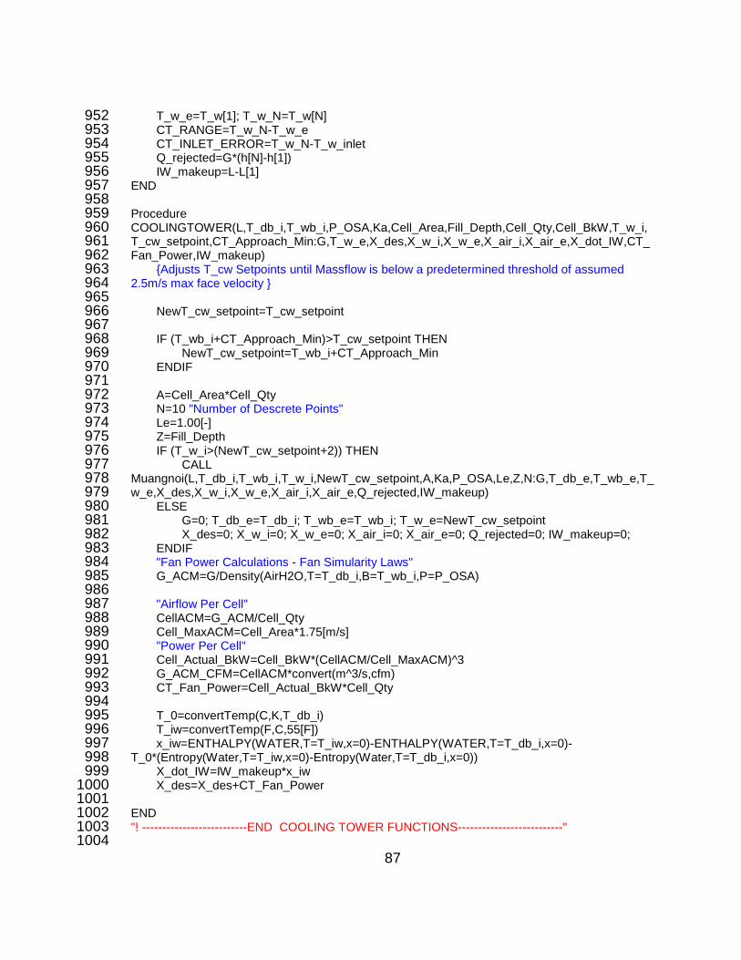
87

T_w_e=T_w[1]; T_w_N=T_w[N] 952 CT_RANGE=T_w_N-T_w_e 953 CT_INLET_ERROR=T_w_N-T_w_inlet 954 Q_rejected=G*(h[N]-h[1]) 955 IW_makeup=L-L[1] 956 END 957 958 Procedure 959 COOLINGTOWER(L,T_db_i,T_wb_i,P_OSA,Ka,Cell_Area,Fill_Depth,Cell_Qty,Cell_BkW,T_w_i,960 T_cw_setpoint,CT_Approach_Min:G,T_w_e,X_des,X_w_i,X_w_e,X_air_i,X_air_e,X_dot_IW,CT_961 Fan_Power,IW_makeup) 962 Adjusts T_cw Setpoints until Massflow is below a predetermined threshold of assumed 963 2.5m/s max face velocity 964 965 NewT_cw_setpoint=T_cw_setpoint 966 967 IF (T_wb_i+CT_Approach_Min)>T_cw_setpoint THEN 968 NewT_cw_setpoint=T_wb_i+CT_Approach_Min 969 ENDIF 970 971 A=Cell_Area*Cell_Qty 972 N=10 "Number of Descrete Points" 973 Le=1.00[-] 974 Z=Fill_Depth 975 IF (T_w_i>(NewT_cw_setpoint+2)) THEN 976 CALL 977 Muangnoi(L,T_db_i,T_wb_i,T_w_i,NewT_cw_setpoint,A,Ka,P_OSA,Le,Z,N:G,T_db_e,T_wb_e,T_978 w_e,X_des,X_w_i,X_w_e,X_air_i,X_air_e,Q_rejected,IW_makeup) 979 ELSE 980 G=0; T_db_e=T_db_i; T_wb_e=T_wb_i; T_w_e=NewT_cw_setpoint 981 X_des=0; X_w_i=0; X_w_e=0; X_air_i=0; X_air_e=0; Q_rejected=0; IW_makeup=0; 982 ENDIF 983 "Fan Power Calculations - Fan Simularity Laws" 984 G_ACM=G/Density(AirH2O,T=T_db_i,B=T_wb_i,P=P_OSA) 985 986 "Airflow Per Cell" 987 CellACM=G_ACM/Cell_Qty 988 Cell_MaxACM=Cell_Area*1.75[m/s] 989 "Power Per Cell" 990 Cell_Actual_BkW=Cell_BkW*(CellACM/Cell_MaxACM)^3 991 G_ACM_CFM=CellACM*convert(m^3/s,cfm) 992 CT_Fan_Power=Cell_Actual_BkW*Cell_Qty 993 994 T_0=convertTemp(C,K,T_db_i) 995 T_iw=convertTemp(F,C,55[F]) 996 x_iw=ENTHALPY(WATER,T=T_iw,x=0)-ENTHALPY(WATER,T=T_db_i,x=0)-997 T_0*(Entropy(Water,T=T_iw,x=0)-Entropy(Water,T=T_db_i,x=0)) 998 X_dot_IW=IW_makeup*x_iw 999 X_des=X_des+CT_Fan_Power 1000 1001 END 1002 "! --------------------------END COOLING TOWER FUNCTIONS--------------------------" 1003 1004

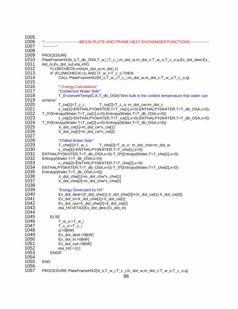
88

1005 "! --------------------------BEGIN PLATE AND FRAME HEAT EXCHANGER FUNCTIONS---------------1006 -----------" 1007 1008 PROCEDURE 1009 PlateFrameHX(N_s,T_db_OSA,T_w_i,T_c_i,m_dot_w,m_dot_c:T_w_o,T_c_o,q,Ex_dot_dest,Ex_1010 dot_in,Ex_dot_out,eta_HX) 1011 FLOWCHECK=min(m_dot_w,m_dot_c) 1012 IF (FLOWCHECK>1) AND (T_w_i>T_c_i) THEN 1013 CALL PlateFrameHX2(N_s,T_w_i,T_c_i,m_dot_w,m_dot_c:T_w_o,T_c_o,q) 1014 1015 "! Exergy Calculations" 1016 "Condensor Water Side" 1017 T_0=convertTemp(C,K,T_db_OSA)"Wet bulb is the coldest temperature that water can 1018 achieve" 1019 T_cw[1]=T_c_i; T_cw[2]=T_c_o; m_dot_cw=m_dot_c 1020 x_cw[1]=ENTHALPY(WATER,T=T_cw[1],x=0)-ENTHALPY(WATER,T=T_db_OSA,x=0)-1021 T_0*(Entropy(Water,T=T_cw[1],x=0)-Entropy(Water,T=T_db_OSA,x=0)) 1022 x_cw[2]=ENTHALPY(WATER,T=T_cw[2],x=0)-ENTHALPY(WATER,T=T_db_OSA,x=0)-1023 T_0*(Entropy(Water,T=T_cw[2],x=0)-Entropy(Water,T=T_db_OSA,x=0)) 1024 X_dot_cw[1]=m_dot_cw*x_cw[1] 1025 X_dot_cw[2]=m_dot_cw*x_cw[2] 1026 1027 "Chilled Water Side" 1028 T_chw[1]=T_w_i; T_chw[2]=T_w_o; m_dot_chw=m_dot_w 1029 x_chw[1]=ENTHALPY(WATER,T=T_chw[1],x=0)-1030 ENTHALPY(WATER,T=T_db_OSA,x=0)-T_0*(Entropy(Water,T=T_chw[1],x=0)-1031 Entropy(Water,T=T_db_OSA,x=0)) 1032 x_chw[2]=ENTHALPY(WATER,T=T_chw[2],x=0)-1033 ENTHALPY(WATER,T=T_db_OSA,x=0)-T_0*(Entropy(Water,T=T_chw[2],x=0)-1034 Entropy(Water,T=T_db_OSA,x=0)) 1035 X_dot_chw[1]=m_dot_chw*x_chw[1] 1036 X_dot_chw[2]=m_dot_chw*x_chw[2] 1037 1038 "Exergy Destroyed by HX" 1039 Ex_dot_dest=(X_dot_chw[1]-X_dot_chw[2])+(X_dot_cw[1]-X_dot_cw[2]) 1040 Ex_dot_in=X_dot_chw[1]+X_dot_cw[1] 1041 Ex_dot_out=X_dot_chw[2]+X_dot_cw[2] 1042 eta_HX=ETA2(Ex_dot_dest,Ex_dot_in) 1043 1044 ELSE 1045 T_w_o:=T_w_i 1046 T_c_o:=T_c_i 1047 q:=0[kW] 1048 Ex_dot_dest:=0[kW] 1049 Ex_dot_in:=0[kW] 1050 Ex_dot_out:=0[kW] 1051 eta_HX:=1[-] 1052 ENDIF 1053 1054 END 1055 1056 PROCEDURE PlateFrameHX2(N_s,T_w_i,T_c_i,m_dot_w,m_dot_c:T_w_o,T_c_o,q) 1057

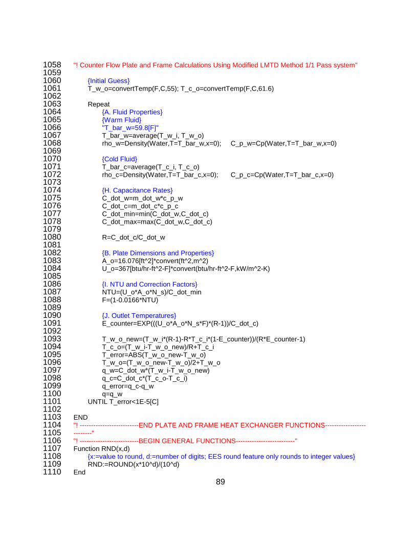
89

"! Counter Flow Plate and Frame Calculations Using Modified LMTD Method 1/1 Pass system" 1058 1059 Initial Guess 1060 T_w_o=convertTemp(F,C,55); T_c_o=convertTemp(F,C,61.6) 1061 1062 Repeat 1063 A. Fluid Properties 1064 Warm Fluid 1065 "T_bar_w=59.8[F]" 1066 T_bar_w=average(T_w_i, T_w_o) 1067 rho_w=Density(Water,T=T_bar_w,x=0); C_p_w=Cp(Water,T=T_bar_w,x=0) 1068 1069 Cold Fluid 1070 T_bar_c=average(T_c_i, T_c_o) 1071 rho_c=Density(Water,T=T_bar_c,x=0); C_p_c=Cp(Water,T=T_bar_c,x=0) 1072 1073 H. Capacitance Rates 1074 C_dot_w=m_dot_w*c_p_w 1075 C_dot_c=m_dot_c*c_p_c 1076 C_dot_min=min(C_dot_w,C_dot_c) 1077 C_dot_max=max(C_dot_w,C_dot_c) 1078 1079 R=C_dot_c/C_dot_w 1080 1081 B. Plate Dimensions and Properties 1082 A_o=16.076[ft^2]*convert(ft^2,m^2) 1083 U_o=367[btu/hr-ft^2-F]*convert(btu/hr-ft^2-F,kW/m^2-K) 1084 1085 I. NTU and Correction Factors 1086 NTU=(U_o*A_o*N_s)/C_dot_min 1087 F=(1-0.0166*NTU) 1088 1089 J. Outlet Temperatures 1090 E_counter=EXP(((U_o*A_o*N_s*F)*(R-1))/C_dot_c) 1091 1092 T_w_o_new=(T_w_i*(R-1)-R*T_c_i*(1-E_counter))/(R*E_counter-1) 1093 T_c_o=(T_w_i-T_w_o_new)/R+T_c_i 1094 T_error=ABS(T_w_o_new-T_w_o) 1095 T_w_o=(T_w_o_new-T_w_o)/2+T_w_o 1096 q_w=C_dot_w*(T_w_i-T_w_o_new) 1097 q_c=C_dot_c*(T_c_o-T_c_i) 1098 q_error=q_c-q_w 1099 q=q_w 1100 UNTIL T_error<1E-5[C] 1101 1102 END 1103 "! --------------------------END PLATE AND FRAME HEAT EXCHANGER FUNCTIONS------------------1104 --------" 1105 "! --------------------------BEGIN GENERAL FUNCTIONS--------------------------" 1106 Function RND(x,d) 1107 x:=value to round, d:=number of digits; EES round feature only rounds to integer values 1108 RND:=ROUND(x*10^d)/(10^d) 1109 End 1110

90

Function ETA2(Xdes,Xin) 1111 Checks to see if Exergy in is not zero to prevent division by zero 1112 IF (RND(Xin,3)=<0) Then 1113 ETA2:=1 1114 ELSE 1115 ETA2:=1-Xdes/Xin 1116 ENDIF 1117 End 1118 Function ETA1(Xout,Xin) 1119 Checks to see if Exergy in is not zero to prevent division by zero 1120 IF (RND(Xin,3)=<0) Then 1121 ETA1:=1 1122 ELSE 1123 ETA1:=Xout/Xin 1124 ENDIF 1125 End 1126 "! --------------------------END GENERAL FUNCTIONS--------------------------" 1127 1128 "! --------------------------BEGIN ECONOMIZER FUNCTIONS--------------------------" 1129 FUNCTION HXTCV(T_CW,T_CHW) 1130 Bypass valving for Heat Exchanger. 1.5[C] is the minimum approach for the HX 1131 IF((T_CW+1[C])<T_CHW) THEN 1132 HXTCV:=0 1133 ELSE 1134 HXTCV:=1 1135 ENDIF 1136 End 1137 FUNCTION CHTCV(T_CHW,T_chws_setpoint) 1138 Bypass valving for Chiller. 1.0[C] is assumed for a deadband range 1139 IF((T_CHW+1[C])<T_chws_setpoint) THEN 1140 CHTCV:=1 1141 ELSE 1142 CHTCV:=0 1143 ENDIF 1144 End 1145 "! --------------------------END ECONOMIZER FUNCTIONS--------------------------" 1146 1147 "! --------------------------BEGIN PROCEEDURE-------------------------" 1148 1149 "Call Modules and Subprograms before main programs" 1150 CALL 1151 MAH(T_db_OSA,T_wb_OSA,P_OSA,T_db_setpoint,T_db_setpoint_low,T_db_setpoint_high, 1152 RH_setpoint,RH_setpoint_low,RH_setpoint_high,MakeUpAir_Min,MAH_BkW_Design,MAH_V_do1153 t_design,MAH_ME_design: MAH_T_db[1..7],MAH_omega[1..7],MAH_Q_preheat, 1154 MAH_Q_humidify, 1155 MAH_Q_cooling_coil,MAH_Q_fan,MAH_FAN_BkW,MAH_X_preheat,MAH_eta_heating,MAH_X_1156 humidify,MAH_eta_humidify,MAH_X_Cooling,MAH_eta_cooling,MAH_X_dest,MAH_X_in,MAH_1157 X_out,MAH_eta_II,MAH_X_dot_air[1..2],MAH_X_dot_hw[1..2], 1158 MAH_X_dot_huw[1],MAH_X_dot_chw[1..2],MAH_X_dot_cd[1]) 1159 1160 CALL CRAH(T_db_OSA, T_wb_OSA, P_OSA,Airflow_RA, MAH_omega[7], T_RA, T_SA, 1161 CRAH_T_chws, P_RA, P_chw, DELTAT_CHW, CRAH_Qty, CRAH_AirFLow, CRAH_BkW: 1162 CRAH_m_dot_chwr, 1163

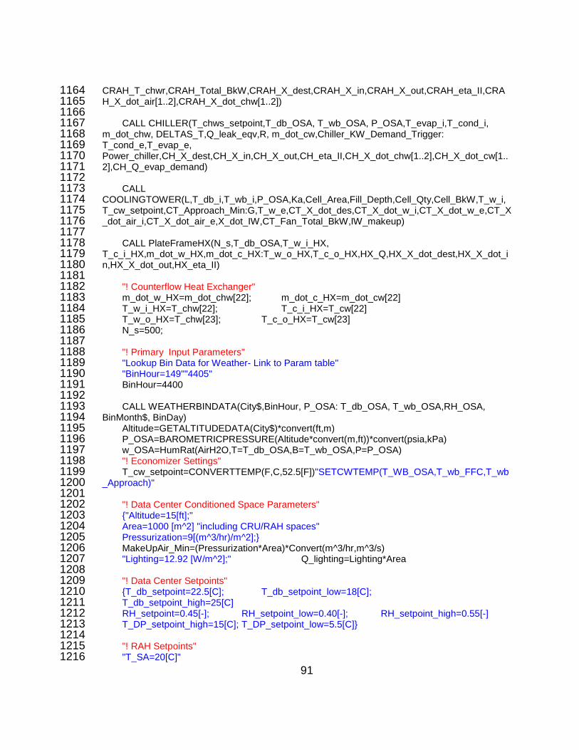
91

CRAH_T_chwr,CRAH_Total_BkW,CRAH_X_dest,CRAH_X_in,CRAH_X_out,CRAH_eta_II,CRA1164 H_X_dot_air[1..2],CRAH_X_dot_chw[1..2]) 1165 1166 CALL CHILLER(T_chws_setpoint,T_db_OSA, T_wb_OSA, P_OSA,T_evap_i,T_cond_i, 1167 m_dot_chw, DELTAS_T,Q_leak_eqv,R, m_dot_cw,Chiller_KW_Demand_Trigger: 1168 T_cond_e,T_evap_e, 1169 Power_chiller,CH_X_dest,CH_X_in,CH_X_out,CH_eta_II,CH_X_dot_chw[1..2],CH_X_dot_cw[1..1170 2],CH_Q_evap_demand) 1171 1172 CALL 1173 COOLINGTOWER(L,T_db_i,T_wb_i,P_OSA,Ka,Cell_Area,Fill_Depth,Cell_Qty,Cell_BkW,T_w_i,1174 T_cw_setpoint,CT_Approach_Min:G,T_w_e,CT_X_dot_des,CT_X_dot_w_i,CT_X_dot_w_e,CT_X1175 _dot_air_i,CT_X_dot_air_e,X_dot_IW,CT_Fan_Total_BkW,IW_makeup) 1176 1177 CALL PlateFrameHX(N_s,T_db_OSA,T_w_i_HX, 1178 T_c_i_HX,m_dot_w_HX,m_dot_c_HX:T_w_o_HX,T_c_o_HX,HX_Q,HX_X_dot_dest,HX_X_dot_i1179 n,HX_X_dot_out,HX_eta_II) 1180 1181 "! Counterflow Heat Exchanger" 1182 m_dot_w_HX=m_dot_chw[22]; m_dot_c_HX=m_dot_cw[22] 1183 T_w_i_HX=T_chw[22]; T_c_i_HX=T_cw[22] 1184 T_w_o_HX=T_chw[23]; T_c_o_HX=T_cw[23] 1185 N_s=500; 1186 1187 "! Primary Input Parameters" 1188 "Lookup Bin Data for Weather- Link to Param table" 1189 "BinHour=149""4405" 1190 BinHour=4400 1191 1192 CALL WEATHERBINDATA(City$,BinHour, P_OSA: T_db_OSA, T_wb_OSA,RH_OSA, 1193 BinMonth$, BinDay) 1194 Altitude=GETALTITUDEDATA(City$)*convert(ft,m) 1195 P_OSA=BAROMETRICPRESSURE(Altitude*convert(m,ft))*convert(psia,kPa) 1196 w_OSA=HumRat(AirH2O,T=T_db_OSA,B=T_wb_OSA,P=P_OSA) 1197 "! Economizer Settings" 1198 T_cw_setpoint=CONVERTTEMP(F,C,52.5[F])"SETCWTEMP(T_WB_OSA,T_wb_FFC,T_wb1199 _Approach)" 1200 1201 "! Data Center Conditioned Space Parameters" 1202 "Altitude=15[ft];" 1203 Area=1000 [m^2] "including CRU/RAH spaces" 1204 Pressurization=9[(m^3/hr)/m^2]; 1205 MakeUpAir_Min=(Pressurization*Area)*Convert(m^3/hr,m^3/s) 1206 "Lighting=12.92 [W/m^2];" Q_lighting=Lighting*Area 1207 1208 "! Data Center Setpoints" 1209 T_db_setpoint=22.5[C]; T_db_setpoint_low=18[C]; 1210 T_db_setpoint_high=25[C] 1211 RH_setpoint=0.45[-]; RH_setpoint_low=0.40[-]; RH_setpoint_high=0.55[-] 1212 T_DP_setpoint_high=15[C]; T_DP_setpoint_low=5.5[C] 1213 1214 "! RAH Setpoints" 1215 "T_SA=20[C]" 1216

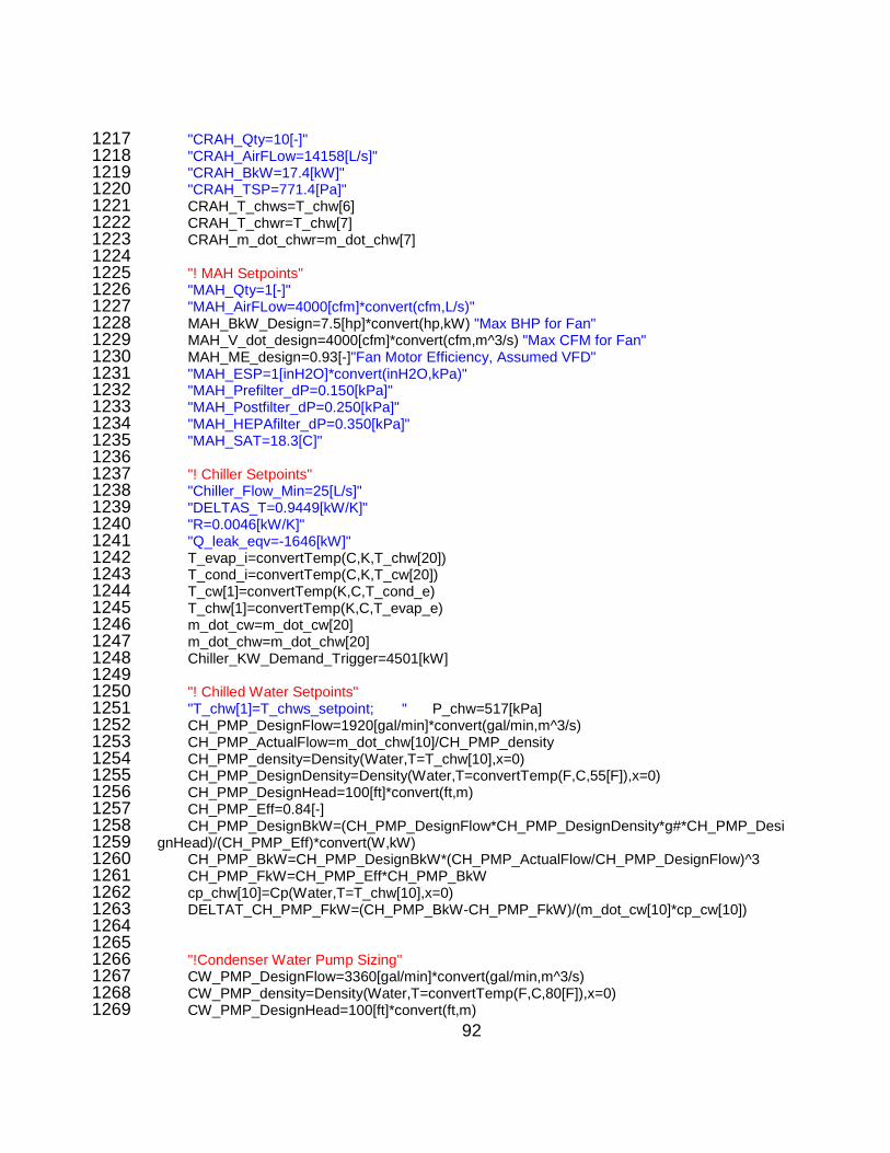
92

"CRAH_Qty=10[-]" 1217 "CRAH_AirFLow=14158[L/s]" 1218 "CRAH_BkW=17.4[kW]" 1219 "CRAH_TSP=771.4[Pa]" 1220 CRAH_T_chws=T_chw[6] 1221 CRAH_T_chwr=T_chw[7] 1222 CRAH_m_dot_chwr=m_dot_chw[7] 1223 1224 "! MAH Setpoints" 1225 "MAH_Qty=1[-]" 1226 "MAH_AirFLow=4000[cfm]*convert(cfm,L/s)" 1227 MAH_BkW_Design=7.5[hp]*convert(hp,kW) "Max BHP for Fan" 1228 MAH_V_dot_design=4000[cfm]*convert(cfm,m^3/s) "Max CFM for Fan" 1229 MAH_ME_design=0.93[-]"Fan Motor Efficiency, Assumed VFD" 1230 "MAH_ESP=1[inH2O]*convert(inH2O,kPa)" 1231 "MAH_Prefilter_dP=0.150[kPa]" 1232 "MAH_Postfilter_dP=0.250[kPa]" 1233 "MAH_HEPAfilter_dP=0.350[kPa]" 1234 "MAH_SAT=18.3[C]" 1235 1236 "! Chiller Setpoints" 1237 "Chiller_Flow_Min=25[L/s]" 1238 "DELTAS_T=0.9449[kW/K]" 1239 "R=0.0046[kW/K]" 1240 "Q_leak_eqv=-1646[kW]" 1241 T_evap_i=convertTemp(C,K,T_chw[20]) 1242 T_cond_i=convertTemp(C,K,T_cw[20]) 1243 T_cw[1]=convertTemp(K,C,T_cond_e) 1244 T_chw[1]=convertTemp(K,C,T_evap_e) 1245 m_dot_cw=m_dot_cw[20] 1246 m_dot_chw=m_dot_chw[20] 1247 Chiller_KW_Demand_Trigger=4501[kW] 1248 1249 "! Chilled Water Setpoints" 1250 "T_chw[1]=T_chws_setpoint; " P_chw=517[kPa] 1251 CH_PMP_DesignFlow=1920[gal/min]*convert(gal/min,m^3/s) 1252 CH_PMP_ActualFlow=m_dot_chw[10]/CH_PMP_density 1253 CH_PMP_density=Density(Water,T=T_chw[10],x=0) 1254 CH_PMP_DesignDensity=Density(Water,T=convertTemp(F,C,55[F]),x=0) 1255 CH_PMP_DesignHead=100[ft]*convert(ft,m) 1256 CH_PMP_Eff=0.84[-] 1257 CH_PMP_DesignBkW=(CH_PMP_DesignFlow*CH_PMP_DesignDensity*g#*CH_PMP_Desi1258 gnHead)/(CH_PMP_Eff)*convert(W,kW) 1259 CH_PMP_BkW=CH_PMP_DesignBkW*(CH_PMP_ActualFlow/CH_PMP_DesignFlow)^3 1260 CH_PMP_FkW=CH_PMP_Eff*CH_PMP_BkW 1261 cp_chw[10]=Cp(Water,T=T_chw[10],x=0) 1262 DELTAT_CH_PMP_FkW=(CH_PMP_BkW-CH_PMP_FkW)/(m_dot_cw[10]*cp_cw[10]) 1263 1264 1265 "!Condenser Water Pump Sizing" 1266 CW_PMP_DesignFlow=3360[gal/min]*convert(gal/min,m^3/s) 1267 CW_PMP_density=Density(Water,T=convertTemp(F,C,80[F]),x=0) 1268 CW_PMP_DesignHead=100[ft]*convert(ft,m) 1269

93

CW_PMP_Eff=0.84[-] 1270 CW_PMP_DesignBkW=(CW_PMP_DesignFlow*CW_PMP_density*g#*CW_PMP_DesignHe1271 ad)/(CW_PMP_Eff)*convert(W,kW) 1272 CW_PMP_BkW=CW_PMP_DesignBkW*(CW_PMP_DesignFlow/CW_PMP_DesignFlow)^3 1273 CW_PMP_FkW=CH_PMP_Eff*CH_PMP_BkW 1274 cp_cw[10]=Cp(Water,T=T_cw[10],x=0) 1275 DELTAT_CW_PMP_FkW=(CW_PMP_BkW-CW_PMP_FkW)/(m_dot_cw[10]*cp_cw[10]) 1276 1277 "!Cooling Tower Setpoint" 1278 CT_Approach_Min=2.8[C] 1279 CT_Approach=T_w_e-T_wb_i 1280 CT_Range=T_w_i-T_w_e 1281 T_db_i=T_db_OSA "Inlet dry-bulb temperature" 1282 T_wb_i=T_wb_OSA "Inlet wet-bulb temperature" 1283 T_w_i=T_cw[6] "Inlet water temperature" 1284 T_w_e=T_cw[7]"T_cw_setpoint" "Exit water temperature" 1285 LG=L/G 1286 1287 CT_X_dot_in=CT_X_dot_air_i+CT_X_dot_w_i+CT_Fan_Total_BkW+X_dot_IW 1288 CT_X_dot_out=CT_X_dot_air_e+CT_X_dot_w_e 1289 CT_eta_II=ETA1(CT_X_dot_out,CT_X_dot_in) 1290 G_ACM=G/Density(AirH2O,T=T_db_i,B=T_wb_i,P=P_OSA) 1291 G_CFM=G_ACM*convert(m^3/s,cfm) 1292 V=Cell_Area*Fill_Depth*Cell_Qty 1293 KaVL=Ka*V/L 1294 m_dot_cw[20]=L "L is set in the Cooling Tower Dialog" 1295 Ka=0.3528 "Cooling Tower Characteristic" 1296 Fill_Depth=7.01[m]"2.4224" 1297 Cell_Area=49.1[m^2] 1298 Cell_Qty=2[-] 1299 Cell_bkW=23[kW] 1300 Cell_MaxACM=2.5[m/s]*Cell_Area; 1301 1302 "! Data Center Airflow Parameters" 1303 "Airflow_bypass=0.30[-]" "Percentage of Air that is bypassed for every CFM of server air" 1304 1305 "! Calculate Heat Load to be Removed" 1306 NRows=4 "Specify number or rows to use in calculating DC Load. Table must be complete" 1307 CALL DATACENTERLOAD(NRows, T_db_setpoint,P_OSA, RH_setpoint: Airflow_Server, 1308 CoolingLoad_DC,Rack) 1309 1310 "! Performance Metrics" 1311 WPSM=CoolingLoad_DC*convert(kW,W)/Area 1312 WPSF=CoolingLoad_DC*convert(kW,W)/(Area*convert(m^2,ft^2)) 1313 Total_Airflow_bypass=Airflow_Server*convert(m^3/s,L/s)*Airflow_bypass 1314 kWPerRack=CoolingLoad_DC/Rack 1315 1316 "! Air Side Flow" 1317 P_RA=P_OSA 1318 Airflow_RA=Airflow_Server+Airflow_bypass 1319 DELTAT_coil=CoolingLoad_DC/(Airflow_RA*Cp(AirH2O,T=T_db_setpoint,w=MAH_omega[71320 ],P=P_RA)*Density(AirH2O,T=T_db_setpoint,w=MAH_omega[7],P=P_RA)) 1321 T_RA=convertTemp(K,C,convertTemp(C,K,T_db_setpoint)+DELTAT_coil) 1322

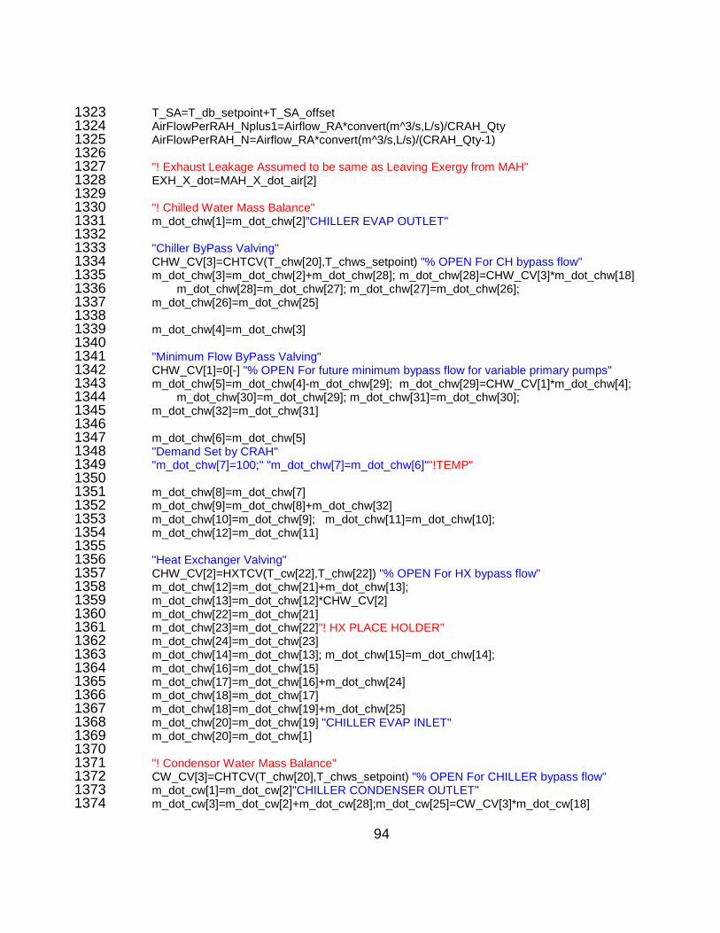
94

T_SA=T_db_setpoint+T_SA_offset 1323 AirFlowPerRAH_Nplus1=Airflow_RA*convert(m^3/s,L/s)/CRAH_Qty 1324 AirFlowPerRAH_N=Airflow_RA*convert(m^3/s,L/s)/(CRAH_Qty-1) 1325 1326 "! Exhaust Leakage Assumed to be same as Leaving Exergy from MAH" 1327 EXH_X_dot=MAH_X_dot_air[2] 1328 1329 "! Chilled Water Mass Balance" 1330 m_dot_chw[1]=m_dot_chw[2]"CHILLER EVAP OUTLET" 1331 1332 "Chiller ByPass Valving" 1333 CHW_CV[3]=CHTCV(T_chw[20],T_chws_setpoint) "% OPEN For CH bypass flow" 1334 m_dot_chw[3]=m_dot_chw[2]+m_dot_chw[28]; m_dot_chw[28]=CHW_CV[3]*m_dot_chw[18] 1335 m_dot_chw[28]=m_dot_chw[27]; m_dot_chw[27]=m_dot_chw[26];1336 m_dot_chw[26]=m_dot_chw[25] 1337 1338 m_dot_chw[4]=m_dot_chw[3] 1339 1340 "Minimum Flow ByPass Valving" 1341 CHW_CV[1]=0[-] "% OPEN For future minimum bypass flow for variable primary pumps" 1342 m_dot_chw[5]=m_dot_chw[4]-m_dot_chw[29]; m_dot_chw[29]=CHW_CV[1]*m_dot_chw[4]; 1343 m_dot_chw[30]=m_dot_chw[29]; m_dot_chw[31]=m_dot_chw[30];1344 m_dot_chw[32]=m_dot_chw[31] 1345 1346 m_dot_chw[6]=m_dot_chw[5] 1347 "Demand Set by CRAH" 1348 "m_dot_chw[7]=100;" "m_dot_chw[7]=m_dot_chw[6]""!TEMP" 1349 1350 m_dot_chw[8]=m_dot_chw[7] 1351 m_dot_chw[9]=m_dot_chw[8]+m_dot_chw[32] 1352 m_dot_chw[10]=m_dot_chw[9]; m_dot_chw[11]=m_dot_chw[10];1353 m_dot_chw[12]=m_dot_chw[11] 1354 1355 "Heat Exchanger Valving" 1356 CHW_CV[2]=HXTCV(T_cw[22],T_chw[22]) "% OPEN For HX bypass flow" 1357 m_dot_chw[12]=m_dot_chw[21]+m_dot_chw[13];1358 m_dot_chw[13]=m_dot_chw[12]*CHW_CV[2] 1359 m_dot_chw[22]=m_dot_chw[21] 1360 m_dot_chw[23]=m_dot_chw[22]"! HX PLACE HOLDER" 1361 m_dot_chw[24]=m_dot_chw[23] 1362 m_dot_chw[14]=m_dot_chw[13]; m_dot_chw[15]=m_dot_chw[14];1363 m_dot_chw[16]=m_dot_chw[15] 1364 m_dot_chw[17]=m_dot_chw[16]+m_dot_chw[24] 1365 m_dot_chw[18]=m_dot_chw[17] 1366 m_dot_chw[18]=m_dot_chw[19]+m_dot_chw[25] 1367 m_dot_chw[20]=m_dot_chw[19] "CHILLER EVAP INLET" 1368 m_dot_chw[20]=m_dot_chw[1] 1369 1370 "! Condensor Water Mass Balance" 1371 CW_CV[3]=CHTCV(T_chw[20],T_chws_setpoint) "% OPEN For CHILLER bypass flow" 1372 m_dot_cw[1]=m_dot_cw[2]"CHILLER CONDENSER OUTLET" 1373 m_dot_cw[3]=m_dot_cw[2]+m_dot_cw[28];m_dot_cw[25]=CW_CV[3]*m_dot_cw[18] 1374

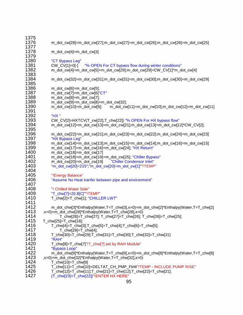
95

1375 m_dot_cw[28]=m_dot_cw[27];m_dot_cw[27]=m_dot_cw[26];m_dot_cw[26]=m_dot_cw[25] 1376 1377 m_dot_cw[4]=m_dot_cw[3] 1378 1379 "CT Bypass Leg" 1380 CW_CV[1]=0[-] "% OPEN For CT bypass flow during winter conditions" 1381 m_dot_cw[4]=m_dot_cw[5]+m_dot_cw[29];m_dot_cw[29]=CW_CV[1]*m_dot_cw[4] 1382 1383 m_dot_cw[32]=m_dot_cw[31];m_dot_cw[31]=m_dot_cw[30];m_dot_cw[30]=m_dot_cw[29] 1384 1385 m_dot_cw[6]=m_dot_cw[5]; 1386 m_dot_cw[7]=m_dot_cw[6]"CT" 1387 m_dot_cw[8]=m_dot_cw[7]; 1388 m_dot_cw[9]=m_dot_cw[8]+m_dot_cw[32]; 1389 m_dot_cw[10]=m_dot_cw[9]; m_dot_cw[11]=m_dot_cw[10];m_dot_cw[12]=m_dot_cw[11] 1390 1391 "HX " 1392 CW_CV[2]=HXTCV(T_cw[22],T_chw[22]) "% OPEN For HX bypass flow" 1393 m_dot_cw[12]=m_dot_cw[13]+m_dot_cw[21];m_dot_cw[13]=m_dot_cw[12]*CW_CV[2]; 1394 1395 m_dot_cw[22]=m_dot_cw[21];m_dot_cw[23]=m_dot_cw[22];m_dot_cw[24]=m_dot_cw[23] 1396 "HX Bypass Leg" 1397 m_dot_cw[14]=m_dot_cw[13];m_dot_cw[15]=m_dot_cw[14];m_dot_cw[16]=m_dot_cw[15] 1398 m_dot_cw[17]=m_dot_cw[16]+m_dot_cw[24]; "HX Return" 1399 m_dot_cw[18]=m_dot_cw[17] 1400 m_dot_cw[18]=m_dot_cw[19]+m_dot_cw[25]; "Chiller Bypass" 1401 m_dot_cw[20]=m_dot_cw[19] "Chiller Condensor Inlet" 1402 "m_dot_cw[20]=215";"m_dot_cw[20]=m_dot_cw[1]""!TEMP" 1403 1404 "!Energy Balance" 1405 "Assume No Heat tranfer between pipe and environment" 1406 1407 "! Chilled Water Side" 1408 "T_chw[7]=20.8[C]""!TEMP" 1409 T_chw[2]=T_chw[1]; "CHILLER LWT" 1410 1411 m_dot_chw[3]*Enthalpy(Water,T=T_chw[3],x=0)=m_dot_chw[2]*Enthalpy(Water,T=T_chw[2]1412 ,x=0)+m_dot_chw[28]*Enthalpy(Water,T=T_chw[28],x=0) 1413 T_chw[28]=T_chw[27]; T_chw[27]=T_chw[26]; T_chw[26]=T_chw[25]; 1414 T_chw[25]=T_chw[18]; 1415 T_chw[4]=T_chw[3];T_chw[5]=T_chw[4];T_chw[6]=T_chw[5]; 1416 T_chw[29]=T_chw[4];1417 T_chw[30]=T_chw[29];T_chw[31]=T_chw[30];T_chw[32]=T_chw[31] 1418 "RAH" 1419 T_chw[8]=T_chw[7]"!T_chw[7] set by RAH Module" 1420 "Bypass Loop" 1421 m_dot_chw[9]*Enthalpy(Water,T=T_chw[9],x=0)=m_dot_chw[8]*Enthalpy(Water,T=T_chw[8]1422 ,x=0)+m_dot_chw[32]*Enthalpy(Water,T=T_chw[32],x=0) 1423 T_chw[10]=T_chw[9] 1424 T_chw[11]=T_chw[10]+DELTAT_CH_PMP_FkW"!TEMP - INCLUDE PUMP RISE" 1425 T_chw[12]=T_chw[11];T_chw[21]=T_chw[12];T_chw[22]=T_chw[21]; 1426 T_chw[23]=T_chw[22]"!ENTER HX HERE" 1427

96

T_chw[24]=T_chw[23]; 1428 1429 T_chw[13]=T_chw[12];T_chw[14]=T_chw[13];T_chw[15]=T_chw[14];T_chw[16]=T_chw[15]; 1430 m_dot_chw[17]*Enthalpy(Water,T=T_chw[17],x=0)=m_dot_chw[16]*Enthalpy(Water,T=T_ch1431 w[16],x=0)+m_dot_chw[24]*Enthalpy(Water,T=T_chw[24],x=0) 1432 T_chw[18]=T_chw[17];T_chw[19]=T_chw[18];T_chw[20]=T_chw[19] 1433 1434 "! Condenser Water Side" 1435 T_cw[2]=T_cw[1] 1436 m_dot_cw[3]*Enthalpy(Water,T=T_cw[3],x=0)=m_dot_cw[2]*Enthalpy(Water,T=T_cw[2],x=0)1437 +m_dot_cw[28]*Enthalpy(Water,T=T_cw[28],x=0) 1438 T_cw[28]=T_cw[27]; T_cw[27]=T_cw[26]; T_cw[26]=T_cw[25];1439 T_cw[25]=T_cw[18]; 1440 T_cw[4]=T_cw[3]; T_cw[5]=T_cw[4];T_cw[6]=T_cw[5] 1441 T_cw[29]=T_cw[4];T_cw[30]=T_cw[29];T_cw[31]=T_cw[30];T_cw[32]=T_cw[31]; 1442 "CT" 1443 T_cw[8]=T_cw[7] 1444 m_dot_cw[9]*Enthalpy(Water,T=T_cw[9],x=0)=m_dot_cw[8]*Enthalpy(Water,T=T_cw[8],x=0)1445 +m_dot_cw[32]*Enthalpy(Water,T=T_cw[32],x=0) 1446 T_cw[10]=T_cw[9] 1447 T_cw[11]=T_cw[10]+DELTAT_CW_PMP_FkW"!TEMP - INCLUDE PUMP RISE" 1448 T_cw[12]=T_cw[11] 1449 T_cw[13]=T_cw[12]; T_cw[14]=T_cw[13]; T_cw[15]=T_cw[14]; T_cw[16]=T_cw[15]; 1450 T_cw[21]=T_cw[12]; T_cw[22]=T_cw[21] 1451 T_cw[23]=T_cw[22] "!ENTER HX HERE" 1452 T_cw[24]=T_cw[23] 1453 m_dot_cw[17]*Enthalpy(Water,T=T_cw[17],x=0)=m_dot_cw[16]*Enthalpy(Water,T=T_cw[16]1454 ,x=0)+m_dot_cw[24]*Enthalpy(Water,T=T_cw[24],x=0) 1455 T_cw[18]=T_cw[17];T_cw[19]=T_cw[18]; 1456 T_cw[20]=T_cw[19] 1457 "T_cw[7]=30;""T_cw[1]=35""!TEMP" 1458 1459 "! Exergy Calculations" 1460 Input=CH_PMP_BkW+CW_PMP_BkW+Power_chiller+CT_Fan_Total_BkW+CRAH_Total_B1461 kW+CT_X_dot_air_i+X_dot_IW+CRAH_X_dot_air[1]+MAH_X_dot_air[1]+MAH_X_dot_hw[1]+MA1462 H_X_dot_huw[1]+MAH_X_dot_chw[1] 1463 Output=CT_X_dot_air_e+EXH_X_dot+MAH_X_dot_hw[2]+MAH_X_dot_chw[2]+MAH_X_dot1464 _cd[1]+CRAH_X_dot_air[2] 1465 eta_II=ETA1(Output,Input) 1466 eta_II_CH_Plant=ETA1(CRAH_X_dot_chw[1]+CT_X_dot_air_e,CH_PMP_BkW+CW_PMP_1467 BkW+Power_chiller+CT_Fan_Total_BkW+X_dot_IW+CRAH_X_dot_chw[2]+CT_X_dot_air_i) 1468 1469 "!SAVE RESULTS TO A TABLE PER SPECIFIED PATH" 1470 "City$='SFO'" 1471 "FileLocation$='X:\SJSU\ME299\Models\'" 1472 1473 FileType$='.LKT ' 1474 FileNameString$=concat$(City$,FileType$) 1475 1476 FileString$=concat$(FileLocation$,FileNameString$) 1477 $SaveTable 'Parametric:AllHours' FileString$ /F 1478