Energy and Carbon Embodied in Exports of Taiwan:

An Input-Output Structural Decomposition Analysis

Shih-Mo Lin, Ya-Tang Chang, Jin-Xu Lin*

This paper computes the energy and carbon intensities of the Taiwanese

economy in 1996, 2001 and 2006 to figure out the changes of energy and carbon

embodied in products and exports and their contributing factors. We use the

structural decomposition analysis to find out the relative contribution of five factors

causing the changes in the energy and carbon embodied in exports. From 1996 to

2001, the changes in the direct energy efficiency, the structure of intermediate inputs

and the structure of exports are the most important factors contributed to the changes

of energy and carbon embodied in exports in Taiwan. On the other hand, the structure

of exports has been the most important factor between 2001 and 2006. This paper

also explores whether energy policy could have effectively reduced the energy and

carbon embodied in exports in Taiwan. Our results of imposing carbon tax on using

fossil fuels reveal that the carbon embodied in exports would have decreased only

moderately from 1996 to 2001 after taxation. However, the carbon embodied in

exports would have decreased significantly from 2001 to 2006 after taxation,

implying that carbon tax would have been a more effective policy in the latter period.

Keywords: embodied carbon, input-output, structural decomposition analysis, carbon

tax

JEL classification: Q48, Q56, F18

* The authors are Professor of Department of International Business, Chung Yuan Christian University, Secretary to Vice

Chairman, Industrial Bank of Taiwan, Associate Professor of Department of International Business, Chung Yuan

Christian University, respectively. Correspondence: Shih-Mo Lin, e-mail: shihmolin@gmail.com; shihmo@cycu.edu.tw.

We are grateful to two anonymous referees and executive editor for their helpful comments. All remaining errors are

ours.

1

1. Introduction

There is an increasing concern about climate change around the world. CO2 is one of the major

greenhouse gases (GHG) causing global warming. According to the 4th

assessment report of the

International Panel on Climate Change (IPCC), CO2 is 76% of the global GHG emissions in 2004

(Lin and Li, 2011). The Taiwan Environmental Protection Administration (EPA) also indicates that

the country’s per capita CO2 emissions are three times higher than that of the global average. Of the

world’s total CO2 emissions, Taiwan is currently ranked 21st in the world (EIA, 2013). Therefore,

efforts to reduce CO2 emissions have become imperative and are gaining momentum all around the

world. Nations are becoming more conscious of their carbon footprints.1 They now compute the

CO2 emissions in the production process of a product.

Due to Taiwan’s geographical position and lack of natural resources, the country has been

focusing on international trade as a source of income. According to the Directorate General of

Budget, Accounting and Statistics (DGBAS), the country’s export earnings in proportion to its GDP

has been increasing from 1981 to 2011. This shows that international trade is becoming a major

economic activity in Taiwan.

A majority of Taiwan's industries rely on fossil fuels which have led to increasing CO2

emissions. IPCC reveals that fossil fuel consumption contributes 56.6% of the CO2 emissions in

Global anthropogenic greenhouse gas emissions in 2004 (4th

Assessment Report of the IPCC; IPCC,

2007). Hence, the environmental impact of fuel combustion has become the main focus in studies

concerning CO2 emissions.

Due to increasing concerns over CO2 emissions, many countries have entered into agreements

to reduce their CO2 emissions. Consequently, if a country is not a signatory of such an agreement,

the member countries can impose a carbon tariff on goods exported by them. Embodied carbon in

commodities may become one of the competitive factors that importing countries will consider in

1 Carbon footprint can be defined as the total direct and indirect CO2 emissions resulting from an activity, organization,

person, or product.

2

the future. Looking at the case of Korea, they are the world’s 10th

largest emitter of energy-related

CO2 as of 2005 (International Energy Agency, 2007). Because of this, they are focusing their efforts

on carbon mitigation initiatives. Such initiatives include putting product labels that indicate how

much carbon was emitted in the manufacturing process, and giving “green cards2” to consumers in

order to encourage the purchase of green products (Low Carbon Green Growth Roadmap for Asia

and the Pacific; United Nations, 2012).

Given the factors mentioned above, the purpose of this paper is to estimate the energy and

carbon embodied in exports of Taiwan and to determine what factors cause the fluctuation of energy

and carbon embodied in exports. Furthermore, this paper aims to simulate the imposition of a

carbon tax on commodities of industries as part of the government’s energy policy, and test whether

it lowers carbon embodied in exports. Previous literatures dealing with the above-mentioned issues

have mostly applied the index decomposition analysis (IDA) or structural decomposition analysis

(SDA). IDA has been applied mainly to aggregate analysis. For example, Greening et al. (1998)

applied the Adaptive Weighted Divisia rolling base year index to figure out the major factors

attributing to the changes of total carbon emissions of the manufacturing sector of 10 OECD

countries for the period 1971-1991. Greening et al. (2001) further applied the same approach to

examine the most important factors which have caused carbon emissions from the residential sector

of 10 OECD countries to change over the 1970-1993 periods. IDA can also be formulated under the

input-output framework. For instance, Chung (1998) and Chung and Rhee (2000) developed

methods to decompose sources of carbon dioxide emissions using a combined index and input–

output approach. The method used by Chung and Rhee (2001) used ‘mean rate-of-change index’ for

weights of the decomposed terms. They claimed that it is particularly useful for decomposing

sources of changes in emissions using the input–output framework, which often involves data set

with negative values (i.e. inventory). However, the major shortcoming of this method is that

2 The Korean Ministry of Environment introduced a green credit card in 2011 to encourage consumers to adopt a more

sustainable lifestyle by providing economic incentives. Points are accumulated as rewards for saving on utility use (tap

water, electricity and gas heating), using public transport, or purchasing eco-friendly products.

3

subjective judgement has inevitably involved in the specification of the weights of the index.

SDA has mostly been specified under the input-output framework to take into account the

direct and indirect industrial linkages among industries of the economy. Different from the IDA

approach, SDA usually does not involve a subjective specification of weights for decomposed terms.

Over the past decades, SDA has been widely applied in energy analysis (Chen and Rose, 1990;

Rose and Chen, 1991), and many studies have even extended it to study the driving forces of carbon

dioxide and other emissions within economies (Casler and Rose, 1998; Chang and Lin, 1998; Liu

and Ang, 2007; Wood and Lenzen, 2009; Liu et al., 2010). In this paper, we follow this trend by

using SDA together with input-output models to conduct our analysis.

The remainder of this paper is organized as follows: Section 2 describes the background of the

energy and carbon embodied in international trade. Section 3 explains the possible effect of a

carbon tax on CO2 emissions. Section 4 shows some methods adopted to calculate the energy and

carbon embodied event. Finally, Section 5 and 6 discusses the empirical results and conclusions,

respectively.

2. Energy and Carbon Embodied in Trade

There has been long-lasting argument regarding the relationship between trade and the environment

over the last several decades. Some analysts argue that trade is inherently good for the environment.

The core of this thought revolves around the law of comparative advantage (Buterbaugh, 2008).

Every region or country is endowed with different mixes of resources, capital and labor. Then, these

different mixes make each region or country better at producing some specific things than others.

However, some analysts advocate trade is bad for the environment. Buterbaugh (2008) listed several

reasons for this inherent conflict. First of all, trade leads to economic growth and which causes a

greater demand for resources, thus harming the environment. Then, free-trade goods are always

shipped over long distances. It is also regarded as damaging the environment. Moreover, many

developing countries do not have the governmental capacity to manage the actions of their citizens

4

or domestic and foreign firms appropriately. Then, free trade may also be seen as one of the reason

for the despoliation of vast area of the developing world. Finally, free trade may arouse the conflict

over resources. Many countries have competed fiercely with each other for controlling different

various resources. All of the reasons above are seen as responsible for harming the environment.

According to the World Trade Organization (WTO), international trade might accelerate the

depletion of natural resources and the degradation of the environment (Nordström and Vaughan,

1999). All goods and services in an economy are directly and/or indirectly associated with energy

use and pollution (Lenzen, 1998; Machado et al., 2001; Peters and Hertwich, 2006). Some studies

also identified three kinds of impacts on the environment and on natural resource related to

international trade.3 These are: scale, composition and technical effects. The energy and pollutant

flows towards and from a country are affected by the mix of exported and imported products, and

the technical efficiency in processing the products and their inputs (Machado et al., 2001).

Furthermore, a country’s fast-growing economy and increased international trade might cause the

over exploitation of resources (Liu et al., 2010). Therefore, a more complete and balanced

information on energy use associated with international trade is needed for all countries across the

globe (Mäenpää and Siikavirta, 2007).

Input-output analysis which has been widely used in analyzing the energy embodied in goods

and services is first designed by Wassily Leontief (1936). Each industry’s production can be

represented by a transaction matrix of intermediate input and final demand through this model.

Then, the application of input-output techniques allows one to trace the direct and indirect

energy/environmental impacts of changes in the final demand (Miller and Blair, 2009; Hawdon and

Pearson, 1995; Kondo et al., 1998; Machado et al., 2001; Liu et al., 2010).

Input-output structural decomposition analysis is a major analytical tool used to study the

observed changes in the level and mix of output. The basic rationale for input-output structural

3 There are three kinds of impacts on the environment and on natural resources related to international trade: scale,

composition and technical effects (OECD, 1997; Nordström and Vaughan, 1999).

5

decomposition analysis is splitting an identity into its components (Rose and Casler, 1998). The

application of structural decomposition analysis is aimed at identifying the driving factors for

change in key variables over time (Casler and Rose, 1998; Ang and Liu, 2001; Wood and Lenzen,

2009). The first formal decomposition of the sources of change in air pollution emissions known to

us is performed by Leontief and Ford in 1972. After Leontief’s pioneering work, energy analysis

has been focused on structural decomposition analysis investigation (Chen and Rose, 1990; Rose

and Chen, 1991), and has examined the mix of output (Pløger, 1984), technology and demand

change (Gowdy and Miller, 1987). Extension of SDA to carbon dioxide emission analysis has since

become a popular field of study (e.g., Casler and Rose, 1998; Chang and Lin, 1998; Liu and Ang,

2007; Wood and Lenzen, 2009; Liu et al., 2010).

3. The Effect of Carbon Tax on CO2 Emissions

Most economists and international organizations have recommended carbon taxes as a

cost-effective instrument for reducing CO2 emissions. Once the tax rate has been set,

emissions-intensive goods will have higher market prices and/or lower profits (Baranzini et al.,

2000). Some researchers estimated the impact of carbon taxes with the different settings of tax rates

on global CO2 emissions (Nordhaus, 1990; Manne and Richels, 1990; Whalley and Wigle, 1991).

All of their results showed that the mitigating effects of carbon taxes are significant. Aasness et al.

(1996) found that a carbon tax rate of $65 per ton of CO2 could let Norway’s CO2 emissions stay at

the 1989 level in 2020 through the general equilibrium approach. Symons et al. (1994) simulated

levying carbon taxes in Britain. The result indicated that carbon taxes would affect the price of

fossil fuels, consumer price, and the level and structure of the UK’s final demand. Nakata and

Lamont (2000), applying the partial equilibrium method, found that carbon and energy taxes would

reduce CO2 emissions to achieve their mitigation goal. It would also encourage the use of gas

instead of coal. Wissema and Dellink (2007) found that levying of carbon tax could also promote

the development of renewable energy. Siriwardena et al. (2007) examined the total extent of CO2

6

mitigation using different levels of price elasticity of demand, and considered the case of Sri

Lanka’s energy and carbon taxes. Using this simulation, they are able to calculate the most effective

carbon tax rate to reduce using carbon-intensive products. Lu et al. (2010) found that carbon taxes

could cut down the carbon emissions in China with the dynamic general equilibrium model, and it

is effective with minimal impact on GDP.

However, the claim that carbon taxes reduce CO2 emissions is controversial. Other studies

show that the mitigating effects of carbon taxes are insignificant due to the tax exemption policies in

certain energy intensive industries (Lin and Li, 2011; Bohlin, 1998). Carbon taxes would induce an

unbalanced burden on industries in countries across Europe (Bordigoni et al., 2012). Morgenstern et

al. (2004) looked at the impacts of a carbon emissions reduction policy on manufacturing industries

in the United States. They found that variations of the tax effect among industries are large which

may be caused by very different tax policies. Furthermore, the simulation yielded a greater

mitigation effect when there's no tax exemption or tax revenue redistribution (Liang et al., 2007).

Nevertheless, if we remove carbon tax exemptions, this may lead to rising levels of global

emissions. It may also influence foreign trade and even social welfare (Harrison and Kristrom, 1997;

Baranzini et al., 2000).

Based on the results of existing studies, the effect of carbon taxes on the international

competitiveness of industries is still controversial. Hence, it is urgent that Taiwan learn more about

energy embodied in exports, and the structure of energy-intensive products or energy efficiency, etc.

so that we can reinforce our energy mitigation policies.

4. Methodology

4.1 Energy Input-Output Analysis

Wassily Leontief integrated the concept of the interaction between industries and the general

equilibrium theory into the input-output analysis. It has been commonly used to analyze the energy

embodied in goods and services and factors causing the changes of energy embodied in industries

7

(Casler and Hannon, 1989; Wu and Chen, 1990; Kagawa and Inamura, 2001; Pan et al., 2008; Liu

et al., 2010).

In the input-output model, total output of an economy is the sum of the intermediate

requirements and the final demand of the economy. Let X represents the total output (column)

vector, A represent the input coefficients matrix, AX is then the sum of the intermediate demand.

With Y being the final demand (column) vector, the following relationship holds (Leontief, 1970):

𝑿 = 𝑨𝑿 + 𝒀 = (𝑰 − 𝑨)−𝟏𝒀 = 𝑳𝒀, (1)

where (I-A)-1

is the Leontief inverse matrix.

The objective of this paper is to analyze the interaction between energy and the economy.

However, if we continue using the original input-output model which uses a standard monetary unit

to express the condition of industries’ energy input, it may have the following drawbacks:

1. Energy prices are highly unstable. Hence, when there are extreme fluctuations in energy prices,

we will not be able to get the actual energy demand of industries under the original model with

the standard monetary units (Chang and Lin, 1998).

2. Using the model with monetary units may not be able to meet the desired level of energy

conservation when calculating industries’ energy input (Chen and Rose, 1990).

This paper adopts the hybrid-unit input-output model developed by Bullard and Herendeen

(1975) to calculate the energy/carbon intensity, which is energy/carbon consumption per unit of

total output of the economy. Under the hybrid-unit input-output analysis, all industrial sectors of the

economy are separated into energy sectors and non-energy sectors. The former is represented by a

physical unit, and the latter is represented by a monetary unit (Bullard and Herendeen, 1975;

Bullard et al., 1978; Miller and Blair, 2009; Park and Heo, 2007).

In the hybrid-unit input-output model, we can define the new transactions matrix Z*, total

output vector X*, and final demand vector Y*. The corresponding matrices are as follows:

𝑨∗ = 𝒁∗(�̂�∗)−𝟏

, (2)

8

𝑳∗ = (𝑰 − 𝑨∗)−𝟏, (3)

where any element in A* is the direct energy/carbon input per unit of total output, elements in Z*

are interindustry transactions, and (�̂�∗)−𝟏

is the inverse of the diagonalized matrix whose diagonal

elements are total output. L* is the total energy/carbon input per unit of total output. Therefore, total

energy/carbon intensity ( ) can be expressed as follows:

𝜶 = 𝑮(�̂�∗)−𝟏𝑳∗, (4)

where 𝑮 is the total output of energy sectors and it is nonzero only for energy sectors. While

𝑮(�̂�∗)−𝟏 is a tool for isolating the energy rows.

4.2 Input-Output Structural Decomposition Analysis

There are a variety of reasons causing the fluctuation of a country’s indirect energy exportation,

such as the growth in the exportation, changes in the international trade structure, technology

progression, and energy efficiency advancement (Hoekstra and van den Bergh, 2002; Liu and Ang,

2007). In this paper, we use the input-output structural decomposition analysis (SDA) to identify

five factors which have contributed to the changes in the energy embodied in exports over time

(Wood and Lenzen, 2009; Liu et al., 2010).

The changes in the energy embodied in exports (∆ 𝑬𝒆𝒙) for sectors can be decomposed into

the changes in total energy intensities (∆𝜶) and changes in exports (∆𝒀𝒆𝒙), as follows:

∆ 𝑬𝒆𝒙 = 𝑬𝒕𝒆𝒙 − 𝑬𝒕−𝟏

𝒆𝒙

= 𝜶𝒕𝒀𝒕𝒆𝒙 − 𝜶𝒕−𝟏𝒀𝒕−𝟏

𝒆𝒙

= (𝜶𝒕𝒀𝒕𝒆𝒙 − 𝜶𝒕−𝟏𝒀𝒕−𝟏

𝒆𝒙 ) − 𝜶𝒕−𝟏𝒀𝒕𝒆𝒙 + 𝜶𝒕−𝟏𝒀𝒕

𝒆𝒙

= (𝜶𝒕 − 𝜶𝒕−𝟏) 𝒀𝒕𝒆𝒙 + 𝜶𝒕−𝟏(𝒀𝒕

𝒆𝒙 − 𝒀𝒕−𝟏𝒆𝒙 )

= ∆𝜶𝒀𝒕−𝟏𝒆𝒙 + 𝜶𝒕∆𝒀𝒆𝒙. (5)

We can find that structure decomposition is additive and non-unique, and it does not include

interaction terms. Therefore, we use the simple average of only two decomposition forms, polar

forms (Dietzenbacher and Los, 1998; Miller and Blair, 2009), to solve the non-uniqueness problem.

9

The changes in the energy embodied in exports are then as follows:

∆ Eex =1

2(∆𝜶)(𝒀𝒕

𝒆𝒙 + 𝒀𝒕−𝟏𝒆𝒙 ) +

1

2(𝜶𝒕 + 𝜶𝒕−𝟏)(∆𝒀𝒆𝒙). (6)

We can use this same method to decompose other fluctuating factors. The changes in the total

energy intensities (∆𝜶) can be decomposed into the changes in direct energy intensities (∆𝒆) and the

Leontief inverse (∆𝑳).

∆𝜶 = 𝒆𝒕𝑳𝒕 − 𝒆𝒕−𝟏𝑳𝒕−𝟏

= ∆𝒆𝑳𝒕−𝟏 + 𝒆𝒕∆𝑳

=𝟏

𝟐(∆𝒆)(𝑳𝒕 + 𝑳𝒕−𝟏) +

𝟏

𝟐(𝒆𝒕 + 𝒆𝒕−𝟏)(∆𝑳). (7)

The changes in the Leontief inverse (∆𝑳) can be further decomposed into the changes in the direct

input-coefficients (∆𝑨𝒕). ∆𝑨𝒕 can also represent the change effects of the structure of intermediate

inputs.

∆𝑳 = 𝑳𝒕 − 𝑳𝒕−𝟏

= (𝑰 − 𝑨𝒕)−𝟏 − (𝑰 − 𝑨𝒕−𝟏)−𝟏

= 𝑳𝒕[(𝑰 − 𝑨𝒕−𝟏) − (𝑰 − 𝑨𝒕)]𝑳𝒕−𝟏

= 𝑳𝒕(𝑨𝒕 − 𝑨𝒕−𝟏)𝑳𝒕−𝟏

= 𝑳𝒕(∆𝑨𝒕)𝑳𝒕−𝟏 . (8)

The structure of exports (𝑭𝒆𝒙) can be expressed as follows:

𝐅𝐞𝐱 =𝐘𝐢

𝐞𝐱

∑ 𝐘𝐢𝐞𝐱 , (9)

where 𝒀𝒊𝒆𝒙 represents the export of the i sector.

Hence, the changes in exports can be decomposed into the changes in the total volume of

exports (∆𝒀𝒔𝒆𝒙) and the structure of exports (∆𝑭𝒆𝒙).

∆𝒀𝒆𝒙 = 𝒀𝒕𝒆𝒙 − 𝒀𝒕−𝟏

𝒆𝒙

= 𝒀𝒔,𝒕𝒆𝒙𝑭𝒕

𝒆𝒙 − 𝒀𝒔,𝒕−𝟏𝒆𝒙 𝑭𝒕−𝟏

𝒆𝒙

= ∆𝒀𝒔𝒆𝒙𝑭𝒕

𝒆𝒙 + 𝒀𝒔,𝒕−𝟏𝒆𝒙 ∆𝑭𝒆𝒙

10

=𝟏

𝟐(∆𝒀𝒔

𝒆𝒙)(𝑭𝒕𝒆𝒙 + 𝑭𝒕−𝟏

𝒆𝒙 ) +𝟏

𝟐(𝒀𝒔,𝒕

𝒆𝒙 + 𝒀𝒔,𝒕−𝟏𝒆𝒙 )(∆𝑭𝒆𝒙). (10)

Direct energy intensity can be expressed (𝒆) as follows:

𝒆 = 𝒅𝒊𝒂𝒈(𝒆𝒔)(𝒅𝒊𝒂𝒈(𝒆𝒔)−𝟏)𝒆 = 𝒅𝒊𝒂𝒈(𝒆𝒔)𝑹, (11)

where 𝑒𝑠 is the sum of direct energy intensity over all industries, and R is the energy intensity

share matrix.

The changes in direct energy intensities (∆𝒆) can be decomposed into the changes in the

energy consumption level (∆𝒆𝒔) and the structure of the energy consumption (∆𝑹):

∆𝒆 = 𝒆𝒕 − 𝒆𝒕−𝟏

= 𝒆𝒔,𝒕′ 𝑹𝒕 − 𝒆𝒔,𝒕−𝟏

′ 𝑹𝒕−𝟏

= ∆𝒆𝒔′ 𝑹𝒕 + 𝒆𝒔,𝒕−𝟏

′ ∆𝑹 = ∆𝒆𝒔′ 𝑹𝒕−𝟏 + 𝒆𝒔,𝒕

′ ∆𝑹

=𝟏

𝟐(∆𝒆𝒔

′ )(𝑹𝒕 + 𝑹𝒕−𝟏) +𝟏

𝟐(𝒆𝒔,𝒕

′ + 𝒆𝒔,𝒕−𝟏′ )(∆𝑹). (12)

As suggested by Dietzenbacher and Los (1998), using the average of two polar forms (as in

(12)) is often an acceptable approach, because using other approaches will inevitably create

additional “interaction” terms, which are usually very difficult to interpret their economic meanings.

Finally, we combined all the separate parts and obtained the following equation for the

decomposition of the energy embodied in exports:

∆ 𝑬𝒆𝒙 = 𝟏𝟖⁄ (∆𝒆𝒔

′ )(𝑹𝒕 + 𝑹𝒕−𝟏)(𝑳𝒕 + 𝑳𝐭−𝟏)(𝒀𝒕𝒆𝒙 + 𝒀𝒕−𝟏

𝒆𝒙 )

+ 𝟏𝟖⁄ (𝒆𝒔,𝒕

′ + 𝒆𝒔,𝒕−𝟏′ )(∆𝑹)(𝑳𝒕 + 𝑳𝒕−𝟏)(𝒀𝒕

𝒆𝒙 + 𝒀𝒕−𝟏𝒆𝒙 )

+ 1 4⁄ (et + et-1) Lt(∆At*)Lt-1 (Yt

ex + Yt-1ex)

+ 𝟏𝟒⁄ (𝜶𝒕 + 𝜶𝒕−𝟏)(∆𝒀𝒔

𝒆𝒔)(𝑭𝒕𝒆𝒙 + 𝑭𝒕−𝟏

𝒆𝒙 )

+ 𝟏𝟒⁄ (𝜶𝒕 + 𝜶𝒕−𝟏)(𝒀𝑺,𝒕

𝒆𝒙 + 𝒀𝑺,𝒕−𝟏𝒆𝒙 )∆𝑭𝒆𝒙 . (13)

According to the above decomposition, the changes in the energy embodied in exports are

caused by the following factors. The changes in the direct energy use of each industry can be

11

shown in the first term on the right-hand side of Eq. (13) and which indicate that the changes in the

energy efficiency of industries. The second term of that equation is shown that the fluctuation of

the share of each energy used directly in each industry which indicate the changes in the structure

of energy consumption of industries. The third term shows that the changes in the structure of

intermediate inputs for each industry. Then, the fourth term shows that the fluctuation of total

volume of exports of industries. Finally, the fluctuation of the share of export volume for each

industry to the total export volume for the whole economy can be shown in fifth term which

represents that the changes in the structure of exports.

4.3 Carbon Tax Analysis

In the input-output price model, we assume that the price of each product is expressed as an index.

In other words, the base year price of each sector is expressed as a percentage. According to the

assumption of input-output analysis, the sum of the supply is equal to the sum of the demand.

Hence, the market price of commodities (𝒑𝒋) is the sum of the input cost (Lee, 2005), as follows:

𝒂𝟏𝟏𝒑𝟏 + 𝒂𝟐𝟏𝒑𝟐 + ⋯ + 𝒂𝒏𝟏𝒑𝒏 + 𝒗𝟏 = 𝒑𝟏

𝒂𝟏𝟐𝒑𝟏 + 𝒂𝟐𝟐𝒑𝟐 + ⋯ + 𝒂𝒏𝟐𝒑𝒏 + 𝒗𝟐 = 𝒑𝟐

𝒂𝟏𝒏𝒑𝟏 + 𝒂𝟐𝒏𝒑𝟐 + ⋯ + 𝒂𝒏𝒏𝒑𝒏 + 𝒗𝒏 = 𝒑𝒏 , (14)

where 𝒂𝒊𝒋 is the input coefficient, 𝒗𝒋 is the primary input coefficient (value added per unit). We

divide the above equations by the commodity prices (𝒑𝒋) on the right-hand side and arrive at the

equation (∑ 𝒂𝒊𝒋𝒊 + 𝒂𝒋𝒗 = 𝟏) represented as the total output, which is equal to the sum of the

intermediate inputs and the primary inputs.

The imposition of the carbon tax would cause the commodity’s price to increase and then

may indirectly cause the change in the input coefficients. This research referred to previous studies

to simulate the fluctuation after the tax imposition with Sweden tax rates ($22.2 U.S. dollars / CO2

per ton) (Liang, 2009; Yang, 2009). We used this carbon tax rate with Leontief price model to

12

calculate the changes in the commodity price after taxation. On the other hand, we also have to

count on energy’s price elasticity of demand with the assumption of fix-total output in order to

calculate the changes in the production quantity of industries.

The primary goal of this section is to measure the energy-demand relationship to revise the

input coefficients of the model after taxation. The methodology of the elasticity estimation referred

to the study of Houthakker et al. (1974), the model is as follows:

𝑸𝒕𝑫 = 𝑸𝒕−𝟏

𝑫 𝜸 + 𝑿𝒕𝜷 + 𝑿𝒕−𝟏𝜶 + 𝜺𝒕 , (15)

where 𝑸𝒕𝑫 is log energy demand in year t, 𝑸𝒕−𝟏

𝑫 is the lag value of log energy demand, 𝑿𝒕 is a set

of measured covariates (e.g. energy prices, population, income, and climate) that affect energy

demand, 𝑿𝒕−𝟏 is the lag values of the covariates, and 𝜺𝒕 is a random error term. The application

study of Bernstein and Griffin (2006) sets demand as a function of prices, income, population and

climate, as follows:

𝑸𝒕𝑫∗

= 𝒇(𝑷𝒕, 𝒀𝒕, 𝑷𝒐𝒑𝒕, 𝑪𝒍𝒊𝒎𝒂𝒕𝒆𝒕) , (16)

where 𝑸𝒕𝑫∗

denotes desired demand in year t. Empirically, due to the possible non-stationarity

property of the variables and the potential cointegrating relationships existing among them, we

conducted unit root and cointegration tests to obtain the long-run price elasticity measures for our

further analysis.4 Please see Table A3-A6 for the variable and data used for estimation, unit root

test results, conintegration test results, as well as the elasticity estimates.

This study used the price elasticity of demand to adjust energy input coefficients in order to

compute the changes in the energy use after taxation. We assumed that the prices of non-energy

sectors were unchanged and the energy use is normally decreasing after tax imposition. Therefore,

we combined the price elasticity of demand and the new commodity prices after taxation to figure

out the fluctuation of industries’ production quantities.

4 In this study, we applied the long-run price elasticity to measure the effects of price change on quantity demand.

The reasons are: (1) input-output tables are annual estimates of the transaction flows of the economy, and the tables we used are those at producers’ prices, which are usually used to capture longer run effects; and (2) our carbon tax analysis is a comparative static one, which measures the completed effects of a policy change.

13

5. Results and Discussions

5.1 Data

Three sets of data are needed for our analysis: input-output tables, energy balance sheets, and CO2

emission coefficients for energies. Input-output tables used in this study are those measured at

producers’ prices and were originally developed by The Directorate General of Budget, Accounting

and Statistics (DGBAS) of Taiwan. The tables have 45, 49, and 52 sectors respectively for year

1996, 2001 and 2006. All the original tables are in current prices. For the purposes of this study,

which intends to analyze the changes in energy and carbon embodied in exports, we need to convert

the tables into constant-price tables. We set year 2006 as our benchmark year and convert the other

two years’ tables into 2006 prices tables.5 To convert the tables into constant-price ones, we did it

separately for domestic and import tables first, and then combine them together. The price indices

used for domestic tables are sectoral output price indices, and the price indices for import ones are

import price indices, all published by DGBAS. However, for primary sectors, construction, and

service industry sectors, there have no published import price indices available. As such, we relied

on sectoral output price indices to complete the conversion process.

In addition to converting all input-output tables into constant-price tables, we also need to

convert the tables with monetary units into hybrid-unit tables, in which all energy inputs to all

sectors are converted from monetary terms into numbers with physical units (BTU in this paper). In

order to compile hybrid-unit input-output tables, we first match up the tables’ sector classification

with those of energy balance sheets and end up with a 33 sectors classification, which comprises 3

primary energy sectors (crude oil, coal, and natural gas), 2 secondary energy sectors (petroleum

products and electricity) and 28 non-energy sectors. Then, we take the energy use data from the

5 After initially converted the tables into constant-price tables, the tables would not be balanced. We further used RAS

method to balance the tables. The boundary conditions used for performing RAS are that all column sums of

intermediate demands are proportionally adjusted to make sure that the sum of all sums is exactly the same as the sum

of all row sums.

14

energy balance sheets to replace the monetary values in input-output tables.6

Energy balance sheets used in the construction of hybrid-unit input-output tables were

developed by the Bureau of Energy (BOE), under the Ministry of Economic Affairs (MOEA) of

Taiwan. After we have constructed our hybrid-unit input-output tables for 1996, 2001 and 2006, we

are ready to perform energy input-output analysis and calculate the energy embodied in exports for

Taiwan for the three years. However, to further calculate carbon embodied in exports, we need to

convert the energy input numbers in the tables from BTU into the volume of CO2 emissions, with

the help of CO2 emission coefficients for all energy types.7 These coefficients are developed by the

GHG8 Emissions Registry of the Environmental Protection Administration (EPA), Taiwan.

5.2 Energy Embodied in Exports

According to the theory of energy input-output analysis presented in previous chapter, the direct and

total energy intensities are the direct and total energy coefficients (A* and L*) in hybrid units

respectively. The direct and total energy coefficients are the direct and total energy inputs per unit of

total output of sectors.

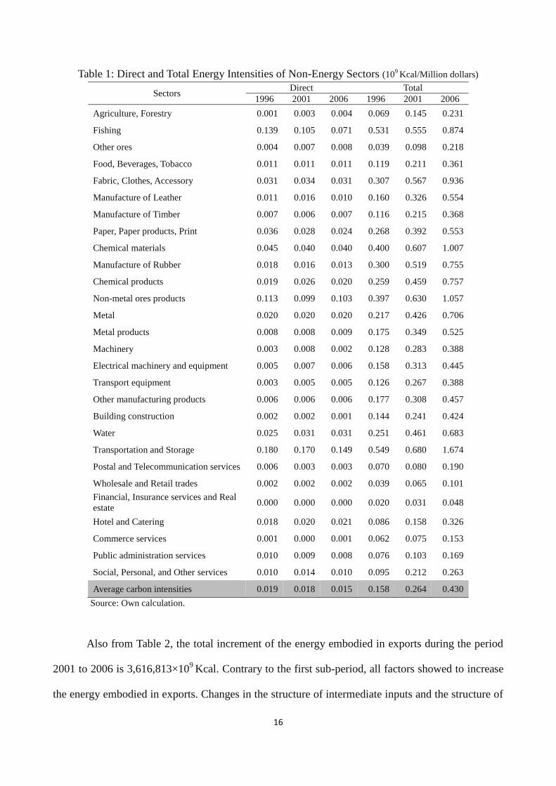
The direct and total energy intensities of sectors for Taiwan in 1996, 2001 and 2006 shown in

Table 1 are measured in 109Kcal/Million dollars.

9 As shown in Table 1, for most of the sectors the

average direct energy intensities of 28 non-energy sectors decreased continuously from 1996 to

2006. The average direct energy inputs is 0.019×109Kcal per unit of total output of the Taiwanese

economy in 1996, 0.018×109Kcal per unit of total output in 2001 and down to 0.015×10

9Kcal per

unit of total output in 2006. On the contrary, the average total energy intensities of 28 non-energy

sectors increased from 1996 to 2001, and increased again from 2001 to 2006. The total energy

inputs is 0.158×109Kcal per unit of total output in 1996, 0.264×10

9Kcal in 2001 and 0.430×10

9Kcal

6 When compiling hybrid-unit input-output tables, it is very important to distinguish between primary and secondary

energy and not to double count the energy used by sectors. Basically, we follow the methodology mentioned in Miller

and Blair (2009) to compile our hybrid-unit tables. 7 In calculating the CO2 emissions, we take into account only those used for generating energy, while those for

non-energy uses are not considered here following the typical rules and steps suggested by EPA and BOE. 8 This stands for greenhouse gases.

9 As mentioned earlier, all results are in 2006 prices.

15

in 2006.

Direct energy intensity decreases and, at the same time, total energy intensity increases means

that the economy is using less energy directly but consuming more energy indirectly. We can see

from Table 1 that chemical materials, non-metal ores and products, and transportation and storage

are the top three sectors with highest total energy intensities. Generally speaking, agricultural

sectors and service sectors have lower total energy intensities, while manufacturing sectors have

higher total energy intensities, which conform to our general intuition.

Using the energy intensity results obtained from the previous section, we are able to calculate

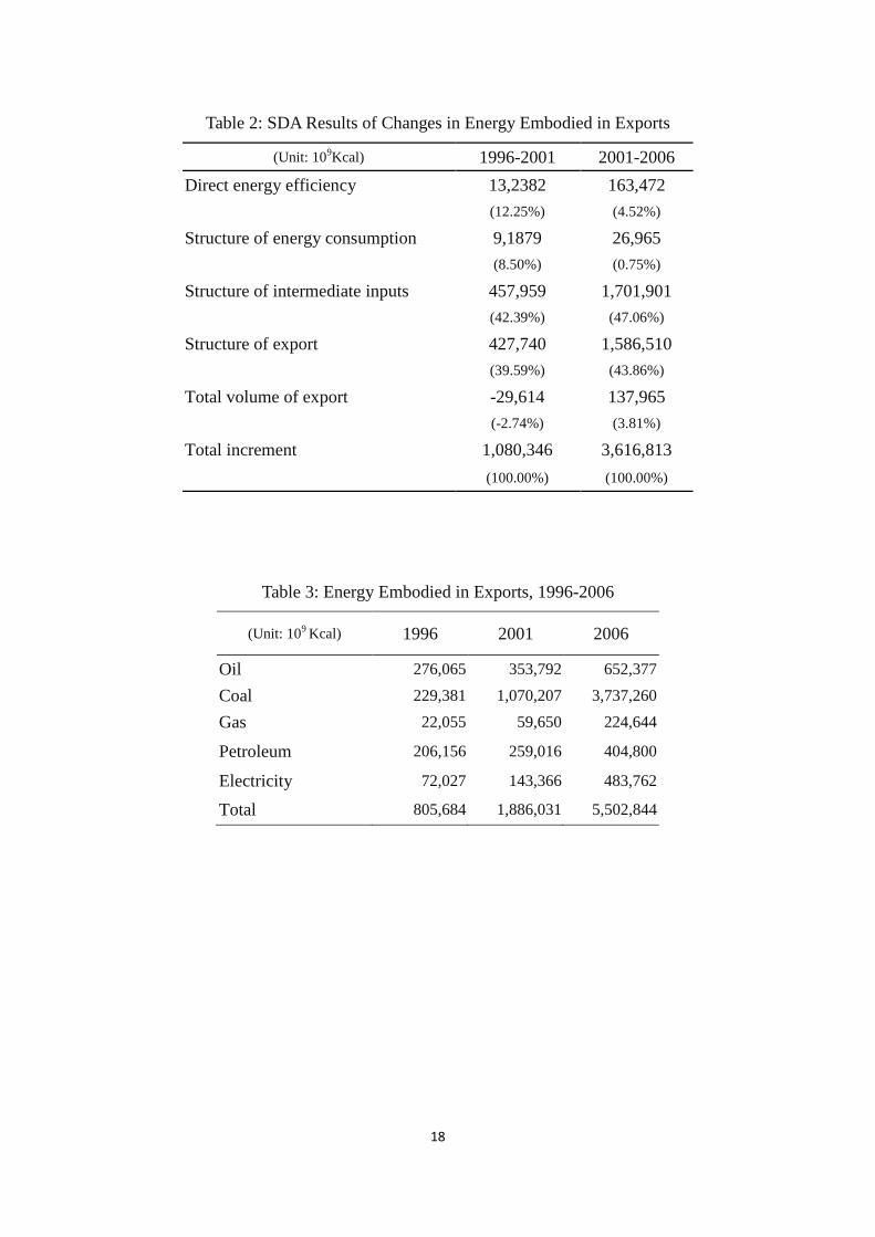
the energy embodied in exports for each of the three years, 1996, 2001 and 2006. According to the

results showed in Table 3, the energy embodied in exports are 805,684×109

Kcal in 1996,

1,886,031×109

Kcal in 2001 and 5,502,884×109

Kcal in 2006, respectively. Energy embodied in

exports for Taiwan increased from 1996 to 2001, and then increased again from 2001 to 2006.

Among those energy used in Taiwan, coal has increased most significantly from 1996 to 2006.

The SDA models presented in the previous section are then applied to analyze the relative

contributions of factors that are responsible for the changes in energy embodied in exports during

the two sub-periods between 1996 and 2006. Results of structural decomposition are shown in Table

2. As revealed in Table 2, the total increment of the energy embodied in exports during 1996 to

2001 is 1,080,346×109

Kcal. Among the five factors, changes in the structure of intermediate inputs

and the structure of exports are the major factors that have contributed to the change of energy

embodied in exports, and the accumulated changes are 42.39% and 39.59%, respectively. The

changes in total volume of exports showed to decrease the energy embodied in exports, and the

accumulated change is -2.74%. This is because that a significant decline in economic outputs was

encountered in 2001 and so did the exports. Moreover, changes in the direct energy efficiency and

energy consumption structure have contributed 12.25% and 8.50% to the accumulated changes,

respectively.

16

Table 1: Direct and Total Energy Intensities of Non-Energy Sectors (109 Kcal/Million dollars)

Sectors Direct Total

1996 2001 2006 1996 2001 2006

Agriculture, Forestry 0.001 0.003 0.004 0.069 0.145 0.231

Fishing 0.139 0.105 0.071 0.531 0.555 0.874

Other ores 0.004 0.007 0.008 0.039 0.098 0.218

Food, Beverages, Tobacco 0.011 0.011 0.011 0.119 0.211 0.361

Fabric, Clothes, Accessory 0.031 0.034 0.031 0.307 0.567 0.936

Manufacture of Leather 0.011 0.016 0.010 0.160 0.326 0.554

Manufacture of Timber 0.007 0.006 0.007 0.116 0.215 0.368

Paper, Paper products, Print 0.036 0.028 0.024 0.268 0.392 0.553

Chemical materials 0.045 0.040 0.040 0.400 0.607 1.007

Manufacture of Rubber 0.018 0.016 0.013 0.300 0.519 0.755

Chemical products 0.019 0.026 0.020 0.259 0.459 0.757

Non-metal ores products 0.113 0.099 0.103 0.397 0.630 1.057

Metal 0.020 0.020 0.020 0.217 0.426 0.706

Metal products 0.008 0.008 0.009 0.175 0.349 0.525

Machinery 0.003 0.008 0.002 0.128 0.283 0.388

Electrical machinery and equipment 0.005 0.007 0.006 0.158 0.313 0.445

Transport equipment 0.003 0.005 0.005 0.126 0.267 0.388

Other manufacturing products 0.006 0.006 0.006 0.177 0.308 0.457

Building construction 0.002 0.002 0.001 0.144 0.241 0.424

Water 0.025 0.031 0.031 0.251 0.461 0.683

Transportation and Storage 0.180 0.170 0.149 0.549 0.680 1.674

Postal and Telecommunication services 0.006 0.003 0.003 0.070 0.080 0.190

Wholesale and Retail trades 0.002 0.002 0.002 0.039 0.065 0.101

Financial, Insurance services and Real

estate 0.000 0.000 0.000 0.020 0.031 0.048

Hotel and Catering 0.018 0.020 0.021 0.086 0.158 0.326

Commerce services 0.001 0.000 0.001 0.062 0.075 0.153

Public administration services 0.010 0.009 0.008 0.076 0.103 0.169

Social, Personal, and Other services 0.010 0.014 0.010 0.095 0.212 0.263

Average carbon intensities 0.019 0.018 0.015 0.158 0.264 0.430

Source: Own calculation.

Also from Table 2, the total increment of the energy embodied in exports during the period

2001 to 2006 is 3,616,813×109

Kcal. Contrary to the first sub-period, all factors showed to increase

the energy embodied in exports. Changes in the structure of intermediate inputs and the structure of

17

exports are still the major factors that contributed to the change of energy embodied in exports, and

the accumulated changes are 47.06% and 43.86%, respectively. Moreover, it is also very interesting

to see from Table 2 that, the change in energy consumption structure has contributed 8.5% to the

accumulated changes of energy embodied in export during the first sub-period, but only 0.75%

during the second sub-period.

For both the two sub-periods, our results show that the contribution of direct energy

efficiency and structure of intermediate inputs have contributed to reduce the energy embodied in

exports, indicating that energy efficiency has improved and production of industries has been

changed towards using more energy-saving technologies in Taiwan. Nevertheless, the contributions

of the structure of exports and total volume of exports have shown to increase the energy embodied

in exports. In particular, the changes in the structure of exports for the two periods have had a big

effect on energy embodied in exports for Taiwan.

While the total increment of energy embodied in exports in the second period (2001 to 2006)

is more than 3 times that of the first period (1996 to 2001), and the changes in the structure of

exports is demonstrated to be the most important factor that has contributed to this change, it would

be needed to check further which sectors are the most responsible ones. To this end, we examined

the structure of exports for the three years, together with the results of total energy intensity of

sectors, to figure out the major sectors causing the change in the energy embodied in exports As

shown in Table 4, the electrical machinery and equipment and the chemical materials sectors are the

two sectors that have significant changes in the share of exports of the economy. Although the total

energy intensity of the former sector is not among the highest, the latter has already been shown to

be one of the most important sectors with high total energy intensity.

18

Table 2: SDA Results of Changes in Energy Embodied in Exports

(Unit: 109Kcal) 1996-2001 2001-2006

Direct energy efficiency 13,2382 163,472

(12.25%) (4.52%)

Structure of energy consumption 9,1879 26,965

(8.50%) (0.75%)

Structure of intermediate inputs 457,959 1,701,901

(42.39%) (47.06%)

Structure of export 427,740 1,586,510

(39.59%) (43.86%)

Total volume of export -29,614 137,965

(-2.74%) (3.81%)

Total increment 1,080,346 3,616,813

(100.00%) (100.00%)

Table 3: Energy Embodied in Exports, 1996-2006

(Unit: 109 Kcal) 1996 2001 2006

Oil 276,065 353,792 652,377

Coal 229,381 1,070,207 3,737,260

Gas 22,055 59,650 224,644

Petroleum 206,156 259,016 404,800

Electricity 72,027 143,366 483,762

Total 805,684 1,886,031 5,502,844

19

Table 4: Structure of Exports in Taiwan, 1996-2006

(Unit: Percent) 1996 2001 2006

Agriculture, Forestry 0.18 0.10 0.06

Fishing 0.80 0.86 0.42

Oil 0.00 0.00 0.00

Coal 0.00 0.00 0.00

Natural gas 0.00 0.00 0.00

Petroleum 0.78 1.63 4.10

Electricity 0.01 0.01 0.00

Other ores 0.04 0.02 0.02

Food, Beverages, Tobacco 2.02 0.70 0.39

Fabric, Clothes, Accessory 9.40 6.72 3.28

Manufacture of Leather 0.90 0.51 0.37

Manufacture of Timber 1.01 0.60 0.23

Paper, Paper products, Print 0.80 0.66 0.61

Chemical materials 3.83 7.13 7.61

Manufacture of Rubber 4.43 2.91 2.56

Chemical products 1.84 1.62 1.11

Non-metal ores products 0.81 0.72 0.38

Metal 2.79 5.18 5.04

Metal products 5.03 5.27 3.72

Machinery 6.33 5.61 5.33

Electrical machinery and equipment 32.56 35.15 42.01

Transport equipment 3.93 2.89 2.99

Other manufacturing products 4.97 2.79 2.83

Building construction 0.10 0.08 0.00

Water 0.00 0.00 0.00

Transportation and Storage 7.15 6.18 4.75

Postal and Telecommunication services 0.53 0.27 0.13

Wholesale and Retail trades 5.12 7.86 8.88

Financial, Insurance services and Real estate 0.38 0.50 0.35

Hotel and Catering 1.42 1.36 0.82

Commerce services 1.89 1.61 0.73

Public administration services 0.00 0.00 0.12

Social, Personal, and Other services 0.95 1.08 1.13

Source: Input-output tables, various years, DGBAS.

20

5.3 Carbon Embodied in Exports

Similar to energy input-output analysis, we perform our carbon embodied in exports and SDA

analysis based on the theory described in previous sections. With the hybrid-unit environmental

input-output tables, the direct and total carbon intensities are the direct and total carbon coefficients

(A* and L*) in hybrid units respectively. The direct and total carbon coefficients are shown as the

direct and total carbon input of per unit of total output of sectors. The results of direct and total

carbon intensities of industries for Taiwan in 1996, 2001 and 2006, shown in tons/Million dollars,10

are presented in Table 5.11

As shown in Table 5, for most of the sectors the average direct carbon intensities of 28

non-energy sectors increased from 1996 to 2001, but decreased from 2001 to 2006. The average

direct carbon embodied is 5.07 tons per unit of total output of the Taiwanese economy in 1996, 5.96

tons per unit of total output in 2001 and down to 5.24 tons per unit of total output in 2006. On the

contrary, the average total carbon intensities of 28 non-energy sectors increased from 1996 to 2001,

and increased again from 2001 to 2006. The total carbon embodied is 45.91 tons per unit of total

output in 1996, 121.64 tons per unit of total output in 2001 and 164.06 tons per unit of total output

in 2006.

Finally, we can see from Table 5 that chemical materials, non-metal ores and products, and

transportation and storage are the top three sectors with highest total carbon intensities. Just like the

results of energy input-output analysis, agricultural sectors and service sectors have lower while

manufacturing sectors have higher total carbon intensities, which also conform to our general

intuition.

10

Again, all results are in 2006 prices. It is very important to know that the CO2 emissions attributable to Taiwan’s

exports for a particular year might not be the numbers shown in the tables. As a recently developed approach by Wang

et al. (2013) suggests, due to the significant increase in intermediate trade, the proportion of domestic value added

embodied in exports has been decreasing. According to Dinh’s (2015) recent research results for Taiwan, the proportion

of domestic value added embodied in exports has decreased from 66.63% in 1995 to 52.24% in 2011. Readers are

advised to take this into account when interpreting our results. Readers are also suggested to consult the detailed

proportions for each sector as shown in Table A2 in the Appendices. 11

Table A1 in Appendices shows the sectoral exports and carbon emissions for all three years. As shown in the table,

electrical machinery and equipment is the most important exporting sector for Taiwan, while Transportation and

Storage sector is the sector emitting most carbon dioxide in Taiwan.

21

Table 5: Direct and Total Carbon Intensities of Non-Energy Sectors (Ton/Million NTD)

Sectors Direct Total

1996 2001 2006 1996 2001 2006

Agriculture, Forestry 0.31 1.06 1.39 18.62 60.99 82.84

Fishing 22.10 32.86 22.45 84.94 213.47 325.51

Other ores 1.34 2.45 2.83 12.22 44.36 82.01

Food, Beverages, Tobacco 3.23 3.54 3.74 35.53 91.62 135.40

Fabric, Clothes, Accessory 9.46 11.35 10.28 106.67 259.12 355.25

Manufacture of Leather 2.97 5.30 5.13 47.67 148.45 223.79

Manufacture of Timber 2.16 2.55 2.51 37.06 117.39 140.74

Paper, Paper products, Print 10.31 9.93 8.71 73.11 175.46 211.01

Chemical materials 14.22 17.37 14.92 119.48 334.26 392.03

Manufacture of Rubber 4.98 5.60 5.44 82.77 253.38 319.97

Chemical products 5.47 8.71 5.13 77.56 223.12 254.64

Non-metal ores products 32.73 36.95 38.67 116.02 303.60 408.94

Metal 5.51 7.39 7.29 62.00 200.93 271.22

Metal products 2.42 2.85 3.23 50.73 161.40 200.76

Machinery 1.01 2.43 0.71 40.50 127.61 148.00

Electrical machinery and equipment 1.52 2.42 2.23 47.46 147.08 173.08

Transport equipment 0.98 1.59 1.74 36.98 129.93 148.63

Other manufacturing products 1.80 1.80 2.11 52.27 144.44 177.27

Building construction 0.50 0.55 0.33 40.11 112.20 161.82

Water 7.76 11.65 11.39 76.02 206.96 265.06

Transportation and Storage 39.73 51.20 45.49 119.98 244.99 614.85

Postal and Telecommunication services 1.15 1.09 1.21 12.18 32.40 69.11

Wholesale and Retail trades 0.60 0.80 0.59 12.82 28.59 37.68

Financial, Insurance services and Real

estate 0.13 0.18 0.15 6.45 14.55 17.73

Hotel and Catering 5.33 5.99 6.20 28.71 65.38 122.27

Commerce services 0.21 0.26 0.31 20.49 48.65 52.87

Public administration services 3.24 2.95 2.66 26.17 43.38 63.85

Social, Personal, and Other services 3.88 3.53 3.66 35.22 71.55 101.61

Average carbon intensities 5.07 5.96 5.24 45.91 121.64 164.06

Source: Own calculation.

Using the carbon intensity results obtained from the previous section, we are able to calculate

the carbon embodied in exports for each of the three years, 1996, 2001 and 2006. According to the

results shown in Table 7, the carbon embodied in exports are 268.54 million tons in 1996, 697.98

million tons in 2001 and 2,103.17 million tons in 2006, respectively. Carbon embodied in exports

22

for Taiwan increased from 1996 to 2001, and then increased again from 2001 to 2006. Among those

energy that emit CO2 in Taiwan, coal has increased significantly from 1996 to 2006. The SDA

models are then applied to analyze the relative contributions of factors that are responsible for the

changes in carbon embodied in exports during the two sub-periods between 1996 and 2006. Results

of structural decomposition are shown in Table 6.

As revealed in Table 6, the total increment of the carbon embodied in exports during 1996 to

2001 is 429.44 million tons. Among the five factors, the structure of intermediate inputs and the

structure of exports are the major factors that have contributed to the change of carbon embodied in

exports, and the accumulated changes are 43.00% and 35.58%, respectively. Also from Table 6, the

changes in total volume of exports revealed to decrease the carbon embodied in exports, and the

accumulated change is -0.05%. Moreover, it is also very interesting to see from Table 6 that, the

change in energy consumption structure has contributed 6.27% to the changes in carbon embodied

in exports during the first sub-period. However, this contribution significantly reduced to -2.37% in

the second sub-period, indicating that energy consumption structure has evolved toward consuming

less energy in the second sub-period.

It can also be seen from Table 6, the total increment of the carbon embodied in exports during

the period 2001 to 2006 is 1,405.19 million tons. Contrary to the first sub-period, the export volume

shown to increase the carbon embodied in exports. Changes in the structure of intermediate inputs

and the structure of exports are still the major factors that have contributed to the change of carbon

embodied in exports, and the accumulated changes are 48.19% and 41.73%, respectively.

Comparing with the results for the two sub-periods, we can see that direct energy efficiency,

energy consumption structure, and structure of intermediate inputs have contributed to the decrease

of the carbon embodied in exports and this indicates that energy efficiency, low carbon energy

development, and production technology of Taiwan have all improved which have led the economy

towards using less energy and, hence, less CO2 emissions. However, the structure of exports and

total volume of exports have shown to have negative effect on the carbon embodied in exports. In

23

particular, the changes in the structure of exports for the two periods have had a big effect on carbon

embodied in exports for Taiwan.

While the total increment of carbon embodied in exports in the second period (2001 to 2006)

is about 3 times that of the first period (1996 to 2001), and the changes in the structure of exports is

demonstrated to be the most important factor that has contributed to this change, it would be helpful

to check further which sectors are most responsible. To this end, we can once again refer to the

structure of exports (Table 4). We can see from the table that the electrical machinery and

equipment and the chemical materials sectors are the two sectors that have significant changes in

the share of exports of the economy. Although the total carbon intensity of the former sector is not

among the highest, the latter has already been shown to be one of the most important sectors with

high total carbon intensity.

5.4 The Effect of Carbon Tax on Carbon Embodied in Exports

In this paper, we would also like to explore how government policy could reduce the energy and

carbon embodied in exports and to what extent. The policy we are considering here is carbon tax.

Levying carbon tax on energy use based on the carbon content of energies will discourage energy

consumption, as the energy cost will go high for almost all sectors of the economy.12

With regard to the level of the carbon tax, we refer to the Sweden carbon tax rate ($22.2 US

dollars/ton CO2) and apply it to the use of primary energy for all sectors. We then use Leontief price

model to calculate the changes in the prices of outputs of all sectors after taxation. We would expect

that imposing carbon tax will lead to an increase in prices for all sectors’ outputs.

12

When the government decides to tax on energy use to comply with international climate change agreements,

expectations arise and agents of the economy will try to adjust beforehand by changing their production and

consumption behavior. With these expectations, the results of taxing on energy use might not exactly the same as we

analyzed, unless we could incorporate expectation behavior into our models. Input-output SDA, being a static analysis

is not suitable to specify the expectation behavior directly into the models. This limitation might thus cause our results

to be slightly overestimated.

24

Table 6: SDA Results of Changes in Carbon Embodied in Exports

(Unit: Million tons CO2) 1996-2001 2001-2006

Direct energy efficiency 65.26 110.35

(15.20%) (7.85%)

Structure of energy consumption 26.94 -33.23

(6.27%) (-2.37%)

Structure of intermediate inputs 184.68 677.19

(43.00%) (48.19%)

Structure of export 152.79 586.38

(35.58%) (41.73%)

Total volume of export -0.22 64.50

(-0.05%) (4.59%)

Total increment 429.44 1405.19

(100.00%) (100.00%)

Table 7: Carbon Embodied in Exports, 1996-2006

(Unit: Million tons CO2) 1996 2001 2006

Oil 80.46 108.57 200.21

Coal 93.98 442.80 1,546.31

Gas 5.08 14.01 52.76

Petroleum 62.36 78.90 123.31

Electricity 26.66 53.69 180.58

Total 268.54 697.98 2,103.17

With the results of price changes for all sectors, we then need to calculate how these changes

will change the direct usage of energy by sectors in their production process. To this end, we make

use of the price elasticities of energy demand for all energy types.13

13

We estimated the price elasticities of demand for oil, coal, natural gas, electricity, and refined petroleum products for

Taiwan, and the data description and estimate results can be found in Table A3, A4, A5, and A6. As can be found in

Table A6, some estimates of price elasticity are not significant (ex. Natural gas). As such, when applying the elasticities

to our calculation of effects we might slightly overestimate the effects. Readers are advised to take this into account

when interpreting the results.

25

Using the percentage change in energy prices together with the price elasticities of energy

demand for all energy types, we can calculate, under the assumption that sectoral outputs remain

constant, the changes in energy inputs by sectors. When total output remains constant and energy

input reduces, the input coefficient of energy for sectors will reduce. This result, combined with the

assumption that other non-energy input coefficients and export levels remain constant, will lead to a

results that the production levels of sectors will decline.

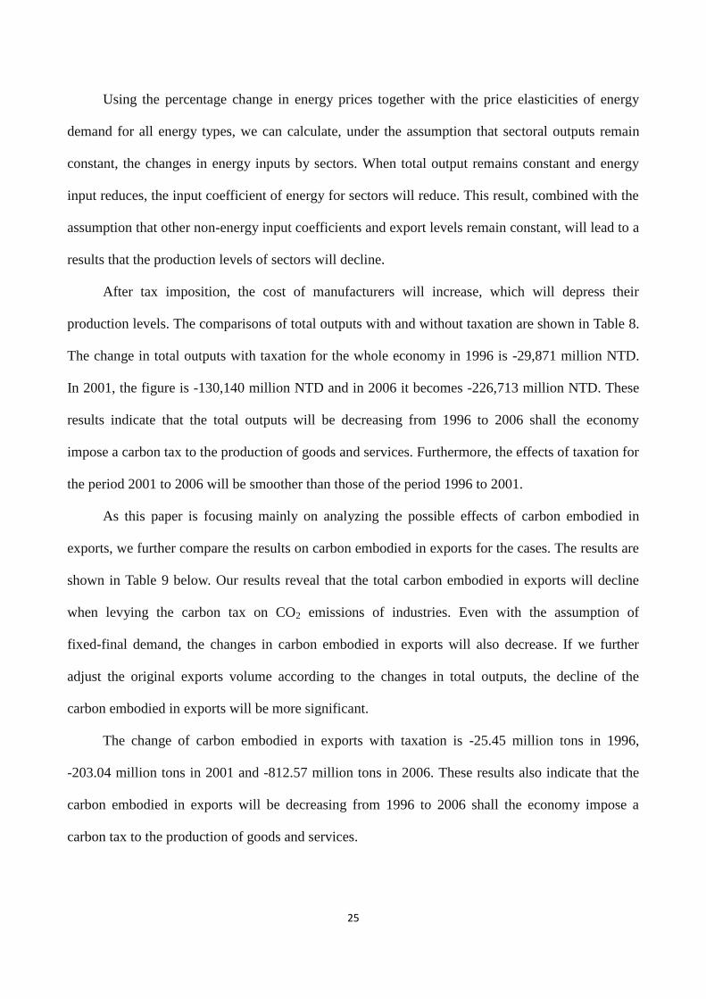
After tax imposition, the cost of manufacturers will increase, which will depress their

production levels. The comparisons of total outputs with and without taxation are shown in Table 8.

The change in total outputs with taxation for the whole economy in 1996 is -29,871 million NTD.

In 2001, the figure is -130,140 million NTD and in 2006 it becomes -226,713 million NTD. These

results indicate that the total outputs will be decreasing from 1996 to 2006 shall the economy

impose a carbon tax to the production of goods and services. Furthermore, the effects of taxation for

the period 2001 to 2006 will be smoother than those of the period 1996 to 2001.

As this paper is focusing mainly on analyzing the possible effects of carbon embodied in

exports, we further compare the results on carbon embodied in exports for the cases. The results are

shown in Table 9 below. Our results reveal that the total carbon embodied in exports will decline

when levying the carbon tax on CO2 emissions of industries. Even with the assumption of

fixed-final demand, the changes in carbon embodied in exports will also decrease. If we further

adjust the original exports volume according to the changes in total outputs, the decline of the

carbon embodied in exports will be more significant.

The change of carbon embodied in exports with taxation is -25.45 million tons in 1996,

-203.04 million tons in 2001 and -812.57 million tons in 2006. These results also indicate that the

carbon embodied in exports will be decreasing from 1996 to 2006 shall the economy impose a

carbon tax to the production of goods and services.

26

Table 8: Outputs with and without Carbon Tax

(Unit: Million NTD) 1996 2001 2006

Before tax 16,486,630 20,669,308 26,910,831

After tax 16,456,759 20,539,168 26,684,117

Total increment -29,871 -130,140 -226,713

Table 9: Carbon Embodied in Exports with and without Carbon Tax

(Unit: Million tons CO2) 1996 2001 2006

Before tax 268.54 697.98 2,103.17

After tax 243.10 494.94 1,290.60

total increment -25.44 -203.04 -812.57

In addition to the above, we can also calculate the carbon embodied in exports for each of the

three years, 1996, 2001 and 2006. As the results in Table 11 indicate, the carbon embodied in

exports after taxation are 237.01 million tons in 1996, 485.70 million tons in 2001 and 1,248.56

million tons in 2006, respectively. Carbon embodied in exports after taxation still matches the

previous trend which increased from 1996 to 2006. Among the energy emitting CO2, coal has

increased most significantly from 1996 to 2006. Comparing with the carbon embodied in exports

before taxation, CO2 emissions of each year all decrease when imposing carbon tax. In order to see

the responsible factors that contribute to the level of carbon embodied in exports after levying

carbon tax, we decompose the change of carbon embodied in exports to analyze the relative

contributions of factors that are responsible for the changes in carbon embodied in exports during

the two sub-periods between 1996 and 2006. Results of structural decomposition are shown in Table

10.

27

Table 10: SDA Results of Factors in Carbon Embodied in Exports with Carbon Tax

(Unit: Million tons CO2) 1996-2001 2001-2006

Direct energy efficiency 33.58 84.58

(13.50%) (11.09%)

Structure of energy consumption 11.31 -38.36

(4.55%) (-5.03%)

Structure of intermediate inputs 86.51 303.78

(34.79%) (39.82%)

Structure of export 116.32 369.26

(46.77%) (48.41%)

Total volume of export 0.97 43.59

(0.39%) (5.71%)

Total increment 248.69 762.86

(100.00%) (100.00%)

Table 11: Carbon Embodied in Exports with Carbon Tax

(Unit: Million tons CO2) 1996 2001 2006

Oil 71.55 91.47 162.57

Coal 80.55 269.46 805.47

Gas 4.75 12.58 42.87

Petroleum 55.28 64.69 92.83

Electricity 24.87 47.50 144.82

Total 237.01 485.70 1,248.56

As revealed in Table 10, the total increment of the carbon embodied in exports after taxation

during 1996 to 2001 is 248.69 million tons. Among the five factors, changes in the structure of

intermediate inputs and the structure of exports are the major factors that have contributed to the

change of carbon embodied in exports, and the accumulated changes are 34.79% and 46.77%,

respectively. The change in total volume of exports is shown to increase slightly by 0.39%. Also

from Table 10, the total increment of the carbon embodied in exports after taxation during the

period 2001 to 2006 is 762.86 million tons. Contrary to the first sub-period, all factors shown to

increase the carbon embodied in exports. Changes in the structure of intermediate inputs and the

28

structure of exports are still the major factors that have contributed to the change of carbon

embodied in exports, and the accumulated changes are 39.82% and 48.41%, respectively.

Furthermore, the change in energy consumption structure has positive contribution to the changes in

carbon embodied in exports during the first sub-period but negative during the second sub-period.

6. Conclusions

International trade is a major economic activity in Taiwan. While there is an increasing concern

about climate change around the world and CO2 has been one of the major greenhouse gases (GHG)

causing global warming, having a good understanding of the energy and carbon embodied in trade

is very important to the government agencies of Taiwan. This paper computed the energy and

carbon intensities of the Taiwanese economy in 1996, 2001 and 2006 to figure out the changes of

energy and carbon embodied in trade and their contributing factors. Our results show that the

chemical materials, non-metal ore and products, and transportation and storage are the top three

sectors with highest total carbon intensities. In particular, direct energy intensity decreases and, at

the same time, total energy intensity increases means that the economy is using less energy directly

but consuming more energy indirectly.

This paper also decomposed the changes into factors causing the changes in the energy and

carbon embodied in exports. Among the five factors considered, changes in the structure of

intermediate inputs and the structure of exports are the major factors that have contributed to the

change of energy and carbon embodied in exports during 1996 to 2001. However, the changes in

energy consumption structure has negative contribution to the changes in carbon embodied in

exports during 2001 and 2006, indicating that the energy consumption structure in Taiwan had

toward more clean energy structure during 1996 and 2006.

The changes in the structure of exports in 2001to 2006 is demonstrated to be the most

important factor that has contributed to the changes in energy and carbon embodied in exports for

that period. After examining the structure of exports, combined with the results for total energy and

29

carbon intensity of sectors, we found that the electrical machinery and equipment and the chemical

materials sector are the two sectors that have significant changes in the share of exports of the

economy. Although the total energy and carbon intensity of the former sector is not among the

highest, the latter has already been shown to be one of the most important sectors with high total

carbon intensity.

The concept of sustainability has been well-taken all over the world. Therefore, the

government should always find out the best way to achieve this goal. In this paper, we also explore

how government policy could have reduced the energy and carbon embodied in exports and to what

extent for Taiwan. Obviously, levying carbon tax on energy use based on the carbon content of

energies will discourage energy consumption, as the energy cost will go high for almost all sectors

of the economy. Our results show that the total outputs would decrease and the carbon embodied in

exports would also decrease from 1996 to 2006. In addition, the SDA results of carbon embodied in

exports after taxation conform to those without taxation between 1996 and 2006.

References

Aasness, Jørgen, Torstein Bye, and Hans Terje Mysen (1996), “Welfare effects of emission taxes in

Norway,” Energy Economics, 18(4), 335-346.

Ang, Beng Wah and Feng Ling Liu (2001), “A new energy decomposition method: perfect in

decomposition and consistent in aggregation, ” Energy, 26(6), 537-548.

Baranzini, Andrea, José Goldemberg, and Stefan Speck (2000), “A future for carbon taxes,”

Ecological Economics, 32(3), 395-412.

Bernstein, Mark A. and James Griffin (2006), Regional Differences in the Price-Elasticity of

Demand for Energy, NREL report.

Bohlin, Folke (1998), “The Swedish carbon dioxide tax: effects on biofuel use and carbon dioxide

emissions,” Biomass and Bioenergy, 15(4-5), 283-291.

Bordigoni, Mathieu, Alain Hita, and Gilles Le Blanc (2012), “Role of embodied energy in the

30

European manufacturing industry: Application to short-term impacts of a carbon tax,”

Energy Policy, 43, 335-350.

Bullard, Clark W. and Robert A. Herendeen (1975), “The energy cost of goods and services,”

Energy Policy, 3(4), 268-278.

Bullard, Clark W., Peter S. Penner, and David A. Pilati (1978), “Net energy analysis: Handbook for

combining process and input-output analysis,” Resources and Energy, 1(3), 267-313.

Buterbaugh, Kevin (2008), “Trade and the environment,” Trade and the Environment, 3, 571-578.

Casler, Stephen D. and Adam Rose (1998), “Carbon dioxide emissions in the US economy: a

structural decomposition analysis,” Environmental and Resource Economics, 11(3-4),

349-363.

Casler, Stephen and Bruce Hannon (1989), “Readjustment potentials in industrial energy efficiency

and structure,” Journal of Environmental Economics and Management, 17(1), 93-108.

Lee, Chang F. and Sue J. Lin (1998), “Structural decomposition of industrial CO2 emission in

Taiwan: an input-output approach,” Energy Policy, 26(1), 5-12.

Chang, Ya-Tang (2013), Energy and Carbon Embodied in International Trade of Taiwan: An

Input-Output Structural Decomposition Analysis, Master Thesis, Department of

International Business, Chung Yuan Christian University.

Chen, Chia-Yon and Adam Rose (1990), “A structural decomposition analysis of changes in energy

demand in Taiwan: 1971-1984,” The Energy Journal, 11(1), 127-146.

Chung, Hyun-Sik (1998), “Industrial structure and source of carbon dioxide emissions in East Asia:

estimation and comparison,” Energy and Environment, 9(5), 509–34.

Chung, Hyun-Sik and Hae-Chun Rhee (2001), “A residual-free decomposition of the sources of

carbon dioxide emissions: a case of the Korean industries,” Energy, 26, 15–30.

Directorate-General of Budget, Accounting and Statistics, Various Years, Input-Output Tables,

Taiwan.

Dietzenbacher, Erik and Bart Los (1998), “Structural decomposition techniques: Sense and

31

sensitivity,” Economic Systems Research, 10, 307-323.

Dinh, Hong Linh (2015), “The value chain transition in east Asian production networks – the view

from value-added decomposition of gross exports,” PhD dissertation, Chung-Li, Taiwan:

PhD Program in Business, Chung Yuan Christian University.

Energy Information Administration/US Department of Energy (2013), “Total carbon dioxide

emissions from the consumption of energy,”

http://www.eia.gov/cfapps/ipdbproject/IEDIndex3.cfm?tid=90&pid=44&aid=8.

Gowdy, John M. and Jamie L. Miller (1987), “Technological and demand change in energy use: an

input-output analysis,” Environment and Planning A, 19(10), 1387-1398.

Greening, Loran A., Willian B. Davis, and Lee Schipper (1998), “Decomposition of aggregate

carbon intensity for the manufacturing sector: comparison of declining trends from 10

OECD countries for the period 1971-1991,” Energy Economics, 20, 43-65.

Greening, Lorna A., Michael Ting, and Thomas J. Krackler (2001), “Effects of changes in

residential end-uses and behavior on aggregate carbon intensity: comparison of 10 OECD

countries for the period 1970 through 1993,” Energy Economics, 23, 153-178.

Harrison, Gleen W. and Bengt Kriström (1997), “Carbon taxes in Sweden,” Institutionen för

Skogsekonomi.

Hawdon, David and Peter Pearson (1995), “Input-output simulations of energy, environment,

economy interactions in the UK,” Energy Economics, 17(1), 73-86.

Hoekstra, Rutger and Jeroen C.J.M. van den Bergh (2002), “Structural decomposition analysis of

physical flows in the economy,” Environmental and Resource Economics, 23(3), 357-378.

Hoekstra, Rutger and Jeroen C.J.M. van den Bergh (2003), “Comparing structural decomposition

analysis and index,” Energy Economics, 25(1), 39-64.

Houthakker, H. S., Philip K. Verleger, Jr., and Dennis P. Sheehan (1974), “Dynamic demand

analyses for gasoline and residential electricity,” American Journal of Agricultural

Economics, 56, 412-418.

32

IEA (2007). Energy Use in the New Millennium: Trends in IEA Countries, IEA, Paris.

Intergovernmental Panel on Climate Change (2007), Climate Change 2007: Synthesis Report,

IPCC, Geneva, Switzerland.

Kagawa, Shigemi and Hajime Inamura (2001), “A structural decomposition of energy consumption

based on a hybrid rectangular input-output framework: Japan's case,” Economic Systems

Research, 13(4), 339-363.

Kondo, Yoshinori, Y. Moriguchi, and H. Shimizu (1998), “CO2 Emissions in Japan: Influences of

imports and exports,” Applied Energy, 59(2), 163-174.

Lee, Kao-Chao (2005), Practices of the input-output analysis (in Chinese), Council for Economic

Planning and Development.

Lenzen, Manfred (1998), “Primary energy and greenhouse gases embodied in Australian final

consumption: an input–output analysis,” Energy Policy, 26(6), 495-506.

Leontief, Wassily (1936), “Quantitative Input and Output Relations in the Economic Systems of

the United States,” The Review of Economics and Statistics, 18(3), 105-125.

Leontief, Wassily (1970), “Environmental repercussions and the economic structure: an

input-output approach,” The Review of Economics and Statistics, 52(3), 262-271.

Liang, Chi-Yuan, (2009), “The effect of energy tax on energy demand and the economy of Taiwan

(in Chinese),” Taiwan Economic Forecast and Policy, 40, 45-78.

Liang, Qiao-Mei, Ying Fan, and Yi-Ming Wei (2007), “Carbon taxation policy in China: How to

protect energy-and trade-intensive sectors? ” Journal of Policy Modeling, 29(2), 311-333.

Lin, Boqiang and Xuehui Li (2011), “The effect of carbon tax on per capita CO2 emissions,”

Energy Policy, 39(9), 5137-5146.

Liu, Hongtao, Youmin Xi, Ju’e Guo, and Xia Li (2010), “Energy embodied in the international

trade of China: An energy input–output analysis,” Energy Policy, 38(8), 3957-3964.

Liu, Na, and Beng Wah Ang (2007), “Factors shaping aggregate energy intensity trend for industry:

Energy intensity versus product mix,” Energy Economics, 29(4), 609-635.

33

Lu, Chuanyi, Qing Tong, and Xuemei Liu (2010), “The impacts of carbon tax and complementary

policies on Chinese economy,” Energy Policy, 38(11), 7278-7285.

Machado, Giovani, Roberto Schaeffer, and Ernst Worrell (2001), “Energy and carbon embodied in

the international trade of Brazil: an input–output approach,” Ecological Economics, 39(3),

409-424.

Madlener, Reinhard, Ronald Bernstein, and Miguel Á ngel Alva González (2011), “Econometric

Estimation of Energy Demand Elasticities,” E.ON Energy Research Center Series, 3(8),

Germany: E.ON Energy Research Center.

Mäenpää, Ilmo and Hanne Siikavirta (2007), “Greenhouse gases embodied in the international

trade and final consumption of Finland: an input–output analysis,” Energy Policy, 35(1),

128-143.

Manne, Alan S. and Richard G. Richels (1990), “CO2 emission limits: an economic cost analysis

for the USA,” The Energy Journal, 11(2), 51-74.

Metz, Bert (2007), Contribution of Working Group III to the Fourth Assessment Report of the

Intergovernmental Panel on Climate Change, Cambridge University Press.

Miller, Ronald E., and Peter D. Blair (2009), Input-output analysis: foundations and extensions,

Cambridge: Cambridge University Press.

Morgenstern, Richard D., Mun Ho, Jhih-Shyang Shih, and Xuehua Zhang (2004), “The near-term

impacts of carbon mitigation policies on manufacturing industries,” Energy Policy, 32(16),

1825-1841.

Nakata, Toshihiko and Alan Lamont (2000), “Analysis of the impacts of carbon taxes on energy

systems in Japan,” Energy Policy, 29(2), 159-166.

Nordhaus, Willian D. (1990), “Global warming: slowing the greenhouse express,” Setting National

Priorities, 192-209.

Nordströmm, Håkan and Scott Vaughan (1999), Trade and the Environment, Special Studies 4,

World Trade Organization.

34

Organization for Economic Co-operation and Development (1997), The Environmental Effects of

Freight, OECD Report.

Pan, Jiahua, Jonathan Phillips, and Ying Chen (2008), “China's balance of emissions embodied in

trade: approaches to measurement and allocating international responsibility,” Oxford

Review of Economic Policy, 24(2), 354-376.

Park, Hi-Chun and Eunnyeong Heo (2007), “The direct and indirect household energy requirements

in the Republic of Korea from 1980 to 2000—an input-output analysis,” Energy Policy,

35(5), 2839-2851.

Peters, Glen P. and Edgar G. Hertwich (2006), “Pollution embodied in trade: The Norwegian case,”

Global Environmental Change, 16(4), 379-387.

Pløger, Ellen (1984), “The effects of structural changes on Danish energy consumption,”

Proceedings of the Fifth IIASA (International Institute for Applied Systems Analysis) Task

Force Meeting on Input–Output Modeling, Laxenburg, Austria, Berlin: Springer-Verlag.

Rose, Adam and Stephen Casler (1996), “Input–output structural decomposition analysis: a critical

appraisal,” Economic Systems Research, 8(1), 33-62.

Rose, Adam and Chia-Yon Chen (1991), “Sources of change in energy use in the US economy,

1972–1982: a structural decomposition analysis,” Resources and Energy, 13(1), 1-21.

Siriwardena, Kanchana, Priyantha D. C. Wijayatunga, W.J.L.S. Fernando, Ran M. Shrestha, and

Rahula A. Attalage (2007), “Economy wide emission impacts of carbon and energy tax in

electricity supply industry: A case study on Sri Lanka,” Energy Conversion and

Management, 48(7), 1975-1982.

Symons, Elizabeth, John Proops, and Philip Gay (1994), “Carbon taxes, consumer demand and

carbon dioxide emissions: a simulation analysis for the UK,” Fiscal Studies, 15(2), 19-43.

United Nations (2012), Low Carbon Green Growth Roadmap for Asia and the Pacific, UN ESCAP

Report.

Wang. Zhi, Shang-Jin Wei, and Kunfu Zhu (2013), “Quantifying international production sharing at

35

the bilateral and sector levels,” NBER Working Paper Series 19677.

Whalley, John and Randall Wigle (1991), “Cutting CO2 emissions: The effects of alternative policy

approaches,” The Energy Journal, 12(1), 109-124.

Wissema, Wiepke and Rob Dellink (2007), “AGE analysis of the impact of a carbon energy tax on

the Irish economy,” Ecological Economics, 61(4), 671-683.

Wood, Richard and Manfred Lenzen (2009), “Structural path decomposition,” Energy Economics,

31(3), 335-341.

Wu, Rong-Hwa and Chia-Yon Chen (1990), “On the application of input-output analysis to energy

issues,” Energy Economics, 12(1), 71-76.

Yang, Hao-Yen (2009), “Economic effects of energy taxation: A computable general equilibrium

analysis in the presence of parameter uncertainty (in Chinese),” Taiwan Economic Forecast

and Policy, 40, 79-125.

36

Appendices

Table A1: Exports and Direct Carbon Emission of Non-Energy Sectors

Sectors

Export

(Billion NTD in 2006 prices)

Direct Carbon Emission

(Thousand tons CO2)

1996 2001 2006 1996 2001 2006

1 Agriculture, Forestry 6 5 5 146 393 507

2 Fishing 29 44 35 3,306 2,731 1,941

3 Other ores 1 1 2 146 215 221

4 Food, Beverages, Tobacco 73 36 33 2,259 2,207 2,153

5 Fabric, Clothes, Accessory 340 342 272 6,287 6,841 5,147

6 Manufacture of Leather 32 26 31 186 204 175

7 Manufacture of Timber 36 30 19 209 170 168

8 Paper, Paper products, Print 29 34 50 3,596 3,035 3,121

9 Chemical materials 139 363 633 12,314 18,955 24,223

10 Manufacture of Rubber 160 148 213 2,124 2,224 2,091

11 Chemical products 67 82 92 1,655 2,390 2,059

12 Non-metal ores products 29 36 32 10,631 8,468 10,151

13 Metal 101 264 419 7,060 9,158 10,735

14 Metal products 182 268 310 1,532 1,721 2,214

15 Machinery 229 286 444 542 1,278 591

16 Electrical machinery and

equipment

1,177 1,791 3,494 2,387 6,119 9,856

17 Transport equipment 142 147 249 545 723 1,066

18 Other manufacturing products 180 142 236 465 384 636

19 Building construction 4 4 0 669 624 415

20 Water 0 0 0 300 374 423

21 Transportation and Storage 258 315 395 35,133 39,755 44,836

22 Postal and

Telecommunication services

19 14 11 239 412 491

23 Wholesale and Retail trades 185 401 739 1,008 1,616 2,010

24 Financial, Insurance services

and Real estate

14 25 29 239 427 396

25 Hotel and Catering 51 69 68 1,234 1,851 2,874

26 Commerce services 68 82 60 93 179 312

27 Public administration services 0 0 10 2,972 2,998 3,204

28 Social, Personal, and Other

services

34 55 94 5,682 7,188 8,940

37

Table A2: Proportion of Domestic Value Added Embodied in Exports, by Sector

1996 2001 2006 2011

Agriculture, Hunting, Forestry and Fishing 83.26 81.94 76.32 73.73

Mining and Quarrying 83.83 85.05 81.18 92.69

Food, Beverages and Tobacco 76.51 77.39 72.65 66.60

Textiles and Textile Products 70.94 75.17 68.62 64.24

Leather, Leather and Footwear 73.36 81.19 69.24 64.31

Wood and Products of Wood and Cork 64.43 65.24 63.27 61.62

Pulp, Paper, Paper , Printing and Publishing 72.98 72.60 65.58 63.86

Coke, Refined Petroleum and Nuclear Fuel 53.30 48.10 26.92 20.96

Chemicals and Chemical Products 63.12 60.77 48.12 49.17

Rubber and Plastics 69.23 69.98 57.76 54.71

Other Non-Metallic Mineral 77.67 74.18 65.37 58.10

Basic Metals and Fabricated Metal 68.82 68.81 55.35 49.84

Machinery, Nec 70.13 70.76 60.75 57.30

Electrical and Optical Equipment 57.90 56.51 49.11 51.06

Transport Equipment 70.84 71.10 61.67 59.57

Manufacturing, Nec; Recycling 75.57 81.92 65.29 60.14

Electricity, Gas and Water Supply 78.96 71.93 52.00 32.69

Construction 74.85 72.14 67.12 61.95

Wholesale and Retail Trade 95.85 93.82 93.93 93.72

Hotels and Restaurants 95.38 95.26 91.47 89.90

Transport 74.65 70.54 57.85 54.93

Other Services 88.49 87.07 85.80 84.60

Weighted average 67.64 65.40 53.58 52.24

38

Table A3: Data Description and Sources for Elasticity Estimation

Variable Description Unit Source

Q_OIL Imported volume of

crude oil

1000 barrels Bureau of Foreign Trade

(BOFT), Ministry of

Economic Affairs

Q_GAS Imported volume of

liquid natural gas

1000 m3

BOFT

Q_COAL Imported volume of

coal

metric ton (mt) BOFT

Q_PETRO Refined petroleum

products consumption

KLOE Bureau of Energy (BOE),

Ministry of Economic

Affairs

Q_ELEC Electricity

consumption

Million kWh BOE

P_OIL Imported crude oil

price

NT$/barrel BOFT

P_GAS Imported gas price NT$/ m3 BOFT

P_COAL Imported Coal price NT$/mt BOFT

P_PETRO Domestic petroleum

price index

index BOE

P_ELEC Domestic electricity

price

NT$/kWh Taipower company

INCOME National income million NT$ DGBAS

POP Population person Directorate General of

Budget, Accounting and

Statistics (DGBAS)

Note: Annual data is from 1991 to 2014. In the study, we use logarithmic transformed variables when estimating the

price elasticity.

39

Figure A1: Population and national income of Taiwan

Figure A2: Import volume and import price of crude oil for Taiwan

Figure A3: Import volume and import price of liquid natural gas for Taiwan

0

2

4

6

8

10

12

14

16

18

19

20

21

22

23

24

1990 1995 2000 2005 2010

Trillion NTD Million people Population National Income

0

20

40

60

80

100

120

0

50

100

150

200

250

300

350

400

450

1990 1995 2000 2005 2010

USD/ barrel Million barrel Q_OIL P_OIL

0

100

200

300

400

500

600

700

800

900

0

2

4

6

8

10

12

14

1990 1995 2000 2005 2010

USD/m3 Billion m3 Q_GAS P_GAS

40

Figure A4: Import volume and import price of coal for Taiwan

Figure A5: Consumption volume and price of electricity for Taiwan

Figure A6: Consumption volume and price index of refined petroleum products for Taiwan

0

20

40

60

80

100

120

140

0

10

20

30

40

50

60

1990 1995 2000 2005 2010

USD/t Million ton Q_COAL P_COAL

0

0.5

1

1.5

2

2.5

3

3.5

0

50

100

150

200

250

300

1990 1995 2000 2005 2010

NTD/kWh Billion kWh Q_ELEC P_ELEC

0

20

40

60

80

100

120

140

0

2

4

6

8

10

12

14

16

1990 1995 2000 2005 2010

index Million KLOE Q_PETRO P_PETRO

41

Estimation Results for Price Elasticities

To estimate the price elasticities for energy products, we test the stationarity of the variables

first and the results are shown in Table A4. As the table indicates, all variables (in logarithmic form)

are integrated of degree one (except for POP using DF-GLS). Based on these results, we then

conduct cointegration tests to examine whether there are cointegrating relationships existing among

variables. The method we used is the typical Trace and Maximum Eigenvalue tests based on

maximum likelihood estimation. Our results are shown in Table A5. According to the results, all

energy products revealed to have at least one cointegrating vector, which allows us to examine the

long-run price elasticity based on the estimated coefficients of the vector (Madlener et al., 2011).

The elasticity estimates are shown in Table A6. It can be seen from Table A6 that two out of the five

elasticities are insignificant (i.e. gas and electricity). However, all elasticities have correct sign and

a magnitude which is less than 1, indicating that energy demands are inelastic with respect to price

changes.

Table A4: Unit Root Test Results

ADF test DF-GLS test

Variable Level differences Level differences

Q_OIL -1.985(0) -5.533**

(0) -0.983 (0) -5.190**

(0)

Q_GAS -2.491 (5) -16.919**

(0) 0.438 (4) -5.879**

(0)

Q_COAL 0.271 (3) -4.694**

(1) -1.213 (3) -5.598**

(0)

Q_PETRO 0.724 (1) -2.371* (0) -1.785 (1) -3.068

* (0)

Q_ELEC -0.988 (0) -5.674**

(0) -1.476 (4) -5.932**

(0)

P_OIL -0.207 (0) -4.458**

(0) -2.488 (0) -4.733**

(1)

P_GAS -0.307 (0) -4.614**

(2) -0.392 (0) -4.350**

(0)

P_COAL -0.451 (0) -4.316**

(0) -1.634 (0) -4.454**

(0)

P_PETRO -0.171 (2) -4.495* (1) -1.102 (0) -5.347

** (0)

P_ELEC 3.477 (5) -7.398**

(0) 0.528 (1) -6.410**

(0)

INCOME -2.169 (3) -3.572**

(0) -1.809 (0) -4.609**

(0)

POP -2.154 (4) -3.185**

(0) -1.471 (1) -2.739 (3)

Notes: 1. Annual data is from 1991 to 2014. 2. * denotes significant at the 5% level, ** denotes significant at the 1%

level. 3. Lag lengths (in parentheses) are selected based on the Schwarz criterion (SC). 4. ELEC, OIL, COAL, GAS,

PETRO, INCOME, POP denote Electricity, Crude oil, Coal, Natural gas, petroleum products, GDP, and population,

respectively.

42

Table A5: Cointegration Test Results

Energy product Null hypothesis λTrace λMaximum Eigenvalue

OIL r = 0

r ≤ 1

r ≤ 2

29.49**

9.88

0.14

19.61*

9.75

0.13

GAS r = 0

r ≤ 1

r ≤ 2

71.45**

36.08*

17.52

35.37**

18.56

13.38

COAL r = 0

r ≤ 1

r ≤ 2

61.96**

30.16**

9.07

27.97*

22.00*

9.81

PETRO r = 0

r ≤ 1

r ≤ 2

29.42*

8.00

0.66

21.42*

7.35

0.66

ELEC r = 0 66.15**

37.81**

18.66*

9.48

r ≤ 1 28.34*

r ≤ 2 9.68

Notes: 1. * denotes significant at the 5% level, ** denotes significant at the 1% level. 2. ELEC, OIL, COAL, GAS,

PETRO denote Electricity, Crude oil, Coal, Natural gas, and petroleum products, respectively.

Table A6: Estimated long-run relationships

Energy

product

Cointegrating vector

Ln(Q_) Ln(P_) Ln(Income) Ln(POP) Ln(P_OIL) C

OIL 1.000 0.649**

(0.127)

-0.953**

(0.037)

GAS 1.000 0.393

(0.784)

-2.064**

(0.193)

-0.577

(0.583)

17.796**

(3.833)

COAL 1.000 0.620**

(0.115)

-1.128**

(0.016)

-0.442**

(0.08)

PETRO 1.000 0.388**

(0.139)

-1.107**

(0.037)

ELEC 1.000 0.097

(0.857)

-1.088**

(0.040)

-0.328**

(0.094)

Notes: 1. * denotes significant at the 5% level, ** denotes significant at the 1% level. 2. (．) indicates the standard

errors. 3. ELEC, OIL, COAL, GAS, PETRO denote Electricity, Crude oil, Coal, Natural gas, and petroleum products,

respectively. 4. The choice of whether to add a constant to the cointegrating vector for different energy products is

mainly based on the Schwarz criterion (SC). 5. For OIL, we replace Ln(income) with Ln(POP) to obtain better

estimates, as Ln(income) and Ln(POP) are closely related. 6. Similarly for GAS, PETRO, and ELEC, we add Ln(P_OIL)

(the log of the price of oil) to take into account the substitutability among energy products and to obtain better estimates

of price elasticities.

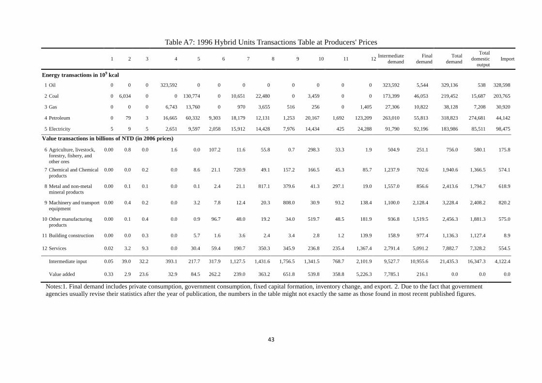
43

Table A7: 1996 Hybrid Units Transactions Table at Producers' Prices

1 2 3 4 5 6 7 8 9 10 11 12 Intermediate

demand

Final

demand

Total

demand

Total

domestic output

Import

Energy transactions in 109 kcal

1 Oil 0 0 0 323,592 0 0 0 0 0 0 0 0 323,592 5,544 329,136 538 328,598

2 Coal 0 6,034 0 0 130,774 0 10,651 22,480 0 3,459 0 0 173,399 46,053 219,452 15,687 203,765

3 Gas 0 0 0 6,743 13,760 0 970 3,655 516 256 0 1,405 27,306 10,822 38,128 7,208 30,920

4 Petroleum 0 79 3 16,665 60,332 9,303 18,179 12,131 1,253 20,167 1,692 123,209 263,010 55,813 318,823 274,681 44,142

5 Electricity 5 9 5 2,651 9,597 2,058 15,912 14,428 7,976 14,434 425 24,288 91,790 92,196 183,986 85,511 98,475

Value transactions in billions of NTD (in 2006 prices)

6 Agriculture, livestock,

forestry, fishery, and

other ores

0.00 0.8 0.0 1.6 0.0 107.2 11.6 55.8 0.7 298.3 33.3 1.9 504.9 251.1 756.0 580.1 175.8

7 Chemical and Chemical

products

0.00 0.0 0.2 0.0 8.6 21.1 720.9 49.1 157.2 166.5 45.3 85.7 1,237.9 702.6 1,940.6 1,366.5 574.1

8 Metal and non-metal mineral products

0.00 0.1 0.1 0.0 0.1 2.4 21.1 817.1 379.6 41.3 297.1 19.0 1,557.0 856.6 2,413.6 1,794.7 618.9

9 Machinery and transport

equipment

0.00 0.4 0.2 0.0 3.2 7.8 12.4 20.3 808.0 30.9 93.2 138.4 1,100.0 2,128.4 3,228.4 2,408.2 820.2

10 Other manufacturing products

0.00 0.1 0.4 0.0 0.9 96.7 48.0 19.2 34.0 519.7 48.5 181.9 936.8 1,519.5 2,456.3 1,881.3 575.0

11 Building construction 0.00 0.0 0.3 0.0 5.7 1.6 3.6 2.4 3.4 2.8 1.2 139.9 158.9 977.4 1,136.3 1,127.4 8.9

12 Services 0.02 3.2 9.3 0.0 30.4 59.4 190.7 350.3 345.9 236.8 235.4 1,367.4 2,791.4 5,091.2 7,882.7 7,328.2 554.5

Intermediate input 0.05 39.0 32.2 393.1 217.7 317.9 1,127.5 1,431.6 1,756.5 1,341.5 768.7 2,101.9 9,527.7 10,955.6 21,435.3 16,347.3 4,122.4

Value added 0.33 2.9 23.6 32.9 84.5 262.2 239.0 363.2 651.8 539.8 358.8 5,226.3 7,785.1 216.1 0.0 0.0 0.0

Notes:1. Final demand includes private consumption, government consumption, fixed capital formation, inventory change, and export. 2. Due to the fact that government

agencies usually revise their statistics after the year of publication, the numbers in the table might not exactly the same as those found in most recent published figures.

44

Table A8: 2001 Hybrid Units Transactions Table at Producers' Prices

1 2 3 4 5 6 7 8 9 10 11 12 Intermediate

demand

Final

demand

Total

demand

Total

domestic output

Import

Energy transactions in 109 kcal

1 Oil 0 0 0 397,673 0 0 0 0 0 0 0 0 397,673 1,469 399,142 366 398,777

2 Coal 0 14,998 0 0 234,379 0 21,717 20,928 0 2,513 0 0 294,534 44,679 339,213 21,561 317,652

3 Gas 0 0 0 4,529 41,276 0 703 3,713 2,356 424 0 1,848 54,850 7,828 62,677 6,793 55,884

4 Petroleum 0 97 0 21,236 55,811 8,318 17,576 10,351 4,795 20,037 1,487 137,643 277,351 67,490 344,841 327,129 17,711

5 Electricity 17 3 471 3,054 12,020 2,150 24,194 17,778 16,286 14,947 467 33,200 124,586 95,122 219,708 127,231 92,478

Value transactions in billions of NTD (in 2006 prices)

6 Agriculture, livestock,

forestry, fishery, and

other ores

0.00 2.5 0.0 1.5 0.0 100.1 14.9 73.5 0.4 243.0 51.0 1.8 488.9 243 732 541 191

7 Chemical and Chemical

products

0.00 0.0 0.7 6.3 6.8 24.1 1,086.3 55.2 299.7 215.4 45.0 122.1 1,861.6 742 2,603 1,940 663

8 Metal and non-metal mineral products

0.00 0.1 0.4 1.5 0.3 4.0 33.0 1,112.3 539.6 66.8 330.2 24.1 2,112.2 550 2,663 2,060 603

9 Machinery and transport

equipment

0.00 0.7 0.3 1.7 15.3 9.2 19.0 26.6 1,377.5 34.1 107.6 173.0 1,764.9 3,233 4,998 3,604 1,395

10 Other manufacturing products

0.00 0.1 0.6 0.5 1.0 77.6 35.4 15.0 39.7 502.1 29.0 207.4 908.4 1,524 2,433 1,838 595

11 Building construction 0.00 0.0 0.9 0.5 7.3 1.6 4.2 3.2 6.6 3.5 1.0 147.5 176.4 968 1,145 1,135 10

12 Services 0.02 3.2 4.6 24.3 19.6 57.1 205.4 289.9 516.4 241.4 184.1 2,055.1 3,601.0 6,605 10,206 9,551 655

Intermediate input 0.07 50.2 39.3 645.4 273.8 307.5 1,702.8 1,704.9 2,827.3 1,367.1 780.4 3,046.2 12,745.1 13,713 26,922 20,000 5,031

Value added 0.22 2.8 18.5 71.2 119.4 233.9 237.6 354.7 776.2 470.9 354.4 6,505.2 9,145.1 191 0 0 0

Note: Final demand includes private consumption, government consumption, fixed capital formation, inventory change, and export.

45

Table A9: 2006 Hybrid Units Transactions Table at Producers' Prices

1 2 3 4 5 6 7 8 9 10 11 12 Intermediate

demand

Final

demand

Total

demand

Total

domestic output

Import

Energy transactions in 109 kcal

1 Oil 0 0 0 522,438 0 0 0 0 0 0 0 0 522,438 -233 522,204 212 521,992

2 Coal 0 16,226 0 0 309,332 0 28,265 24,623 0 2,987 0 0 381,434 43,302 424,736 22,235 402,500

3 Gas 0 0 0 2,592 70,517 0 1,401 4,653 1,947 483 0 3,099 84,693 10,490 95,184 3,704 91,480

4 Petroleum 0 177 0 22,657 45,845 5,638 16,522 11,366 1,751 14,822 805 155,026 274,610 182,409 457,018 430,068 26,951

5 Electricity 72 1 670 3,032 13,909 2,554 30,296 22,380 28,178 14,828 464 41,661 158,044 110,313 268,358 164,455 103,903

Value transactions in billions of NTD (in 2006 prices)

6 Agriculture, livestock,

forestry, fishery, and

other ores

0.00 0.0 0.0 1.1 0.0 93.5 14.9 80.8 0.2 210.6 33.5 17.6 452.1 256 708 529 179

7 Chemical and Chemical

products

0.00 0.1 0.3 6.5 3.9 21.2 1,404.5 71.2 401.2 196.8 42.9 189.7 2,338.3 1,043 3,381 2,394 987

8 Metal and non-metal mineral products

0.00 0.1 0.2 2.7 0.5 2.3 35.2 1,308.6 570.8 58.4 409.7 56.7 2,445.3 847 3,292 2,421 872

9 Machinery and transport

equipment

0.01 1.4 0.5 3.3 13.0 8.8 14.4 25.7 2,555.7 72.2 134.3 230.5 3,059.8 5,531 8,591 5,865 2,725

10 Other manufacturing products

0.00 0.1 0.1 1.0 0.4 69.0 26.4 12.9 53.2 484.3 32.8 316.8 997.2 1,576 2,574 1,852 722

11 Building construction 0.00 0.1 0.6 4.0 1.1 1.7 10.0 9.9 10.6 4.3 1.2 151.2 194.6 1,064 1,259 1,259 0

12 Services 0.02 1.9 4.0 28.9 22.7 58.1 212.1 325.0 843.6 316.2 240.6 2,701.2 4,754.3 8,647 13,402 12,591 811

Intermediate input 0.19 32.4 44.8 908.7 337.1 295.4 2,057.9 1,968.5 4,520.4 1,405.8 912.6 4,094.5 16,578.4 19,553 36,132 28,555 7,577

Value added 0.11 6.6 14.3 128.3 171.5 233.8 336.3 452.1 1,344.8 446.2 346.0 8,496.3 11,976.5 267 0 0 0

Note: Final demand includes private consumption, government consumption, fixed capital formation, inventory change, and export.

46

台灣出口品之能源及碳隱含量：投入產出結構分解分析

林師模．張雅棠．林晉勗*

本文估算台灣 1996、2001 及 2006 年出口品的能源及碳隱含量，以衡量

能源及碳隱含量的變化情形及其影響因素。文中利用結構分解分析將出口品能

源及碳隱含量變化的影響因子區分為五個因子，結果發現在 1996至 2001年間，

能源使用效率、中間財的投入結構，以及出口結構的變化是造成台灣出口品能

源及碳隱含量變化的主要因素；而在 2001 至 2006 年間則是以出口結構的變化

為主要影響因子。此外，本文也同時評估台灣能源政策對減少出口品之能源及

碳隱含量的有效性，研究結果顯示，在 1996 年至 2001 年間，若對化石能源課

徵碳稅僅能微幅降低出口品之能源及碳隱含量，但在 2001 年至 2006 年間卻能

使出口品之能源及碳隱含量明顯的減少，亦即在 2001 年至 2006 年間碳稅政策

較前一段期間來得更有效。

關鍵詞: 碳隱含量、投入產出、結構分解分析、能源稅

JEL 分類代號: Q48, Q56, F18

* 作者分別為中原大學國際經營與貿易學系教授、台灣工業銀行副董事長秘書，與中原大學國際經營與貿易學

系副教授。聯繫作者：林師模，e-mail: shihmolin@gmail.com、shihmo@cycu.edu.tw。作者感謝兩位匿名審查人

及執行編輯的諸多寶貴意見。文中如有任何疏漏，悉屬作者之責。