California Institute for

Energy and Environment

California Institute for

Energy and Environment

E n e r g y R e s e a r c h a n d De v e l o p m e n t Di v i s i o n F I N A L P R O J E C T R E P O R T

ENABLING TECHNOLOGIES DEVELOPMENT GRANT PROGRAM Final Report 2002-2015 Appendices N-R

JUNE 2015 CEC-500-2016 -011-APN -R

Prepared for: California Energy Commission Prepared by: California Institute for Energy and Environment University of California

APPENDIX N Appendix N: Appendix 7: Demand Response Analysis And Control System Phase 1

1.0 Executive Summary

1.1. Project in Brief This document meets the deliverable requirement for Task 5, Develop Final Report for a Demand Response Analysis and Control System (DRACS) for Research Opportunity DR ETD-02-01. The grant was provided to the EnerNex team to address two research topics and questions identified in the opportunity notice:

• “Using a military (or another, such as air traffic control) C3I (Command, Control, Communication, and Information) system as a model, adapt it to conceptually deal with C2I electricity applications such as dispatching DER to keep the lights on. Compare and contrast the chosen C3I model with the requirements for implementing a C2I strategy for integrating utility control, communications and information systems. Are there analogies that indicate utilities can operate in a similar fashion? If not, what are the gaps that need to be filled and is it feasible to fill the gaps?

• Given current utility systems and assuming the systems are integrated, how would the CAISO or an UDC operate its control centers in a military (or another) C3I style? With up-to-date real-time information and the ability to control all of its available assets, given a particular operational scenario, how would a plan to address the scenario be executed using strategies based on military (or another) C3I?”

This report is based on careful studies, close interaction with San Diego Gas & Electric stakeholders, and coordinated efforts between EnerNex Demand Response experts, the Open Smart Grid AMI Enterprise team, and C3I system engineers at Oak Ridge National Laboratories (ORNL).

1.2. Project Approach This project was broken into two phases. The first phase is the research portion of the effort, and this report is directed towards the efforts conducted during the phase one activities. The second phase is proposed for the future, and is discussed in more detail in the Recommendations section of this document.

The first phase of this project consisted of the following tasks and deliverables:

1.2.1. Task 1 – Develop Requirements for a Demand Response Analysis and Control System (DRACS) This task involved the development of traceable and defensible requirements for command and control systems capable of operating systems with high penetrations of demand responsive load. This task utilized the use case based methodology for requirements capture developed by the EPRI IntelliGrid Consortium, the same methodology used at Southern California Edison for the AMI requirements development. The EnerNex team conducted a workshop with utility and industry demand response stakeholders. Where possible, existing use cases, message traffic models, and related information developed for SCE’s AMI project were utilized.

7

Deliverable: DRACS Requirements Document

1.2.2. Task 2 – Develop Requirements for a platform to simulate the behavior of the DRACS This task utilized the same methods for requirements capture applied in Task 1 but for the purpose of determining what information, models, and algorithms are necessary to simulate the behavior of the DRACS. The platform is intended to be used to evaluate the overall stability of the power system when large amounts of demand responsive load change state in short time periods under the control of communication networks with large and highly variable latencies.

Deliverable: DRACS Simulator Requirements Document

1.2.3. Task 3 – DRACS Architecture and Reference Design Development This task involved the creation of an architecture and reference design for a generic DRACS based on the requirements captured in Task 1. The reference design provides discussions of the Demand Response Management System (DRMS) parent system, DRACS design considerations, architectural strategies, the reference architecture and design, and architectural policies and tactics.

Deliverable: DRACS Reference Architecture Document

1.2.4. Task 4 – Simulation and Stability Analysis Platform Framework Development This task developed the framework for a simulation and stability analysis platform suitable for testing a DRACS and evaluating its performance based on the requirements captured in Task 2. This platform will consist of a combination of commercial and freely available software to be configured in a laboratory environment in Phase 2. The document resulting from this task will describe the simulation platform framework, the tools and components that constitute the framework..

Deliverable: DRACS Simulation Framework Document

1.2.5. Task 5 – Phase I Report The Phase 1 report documents the key findings of the Phase 1 research. The focus of the report is to provide background on the activities conducted, provide details on what was learned, and make recommendations for going forward with a Phase 2 effort.

Deliverable: Phase I Final Report Document

8

2.0 Findings and Results The DRACS Phase 1 project provided EnerNex team members with the opportunity to talk with many demand response experts and incorporate the EPRI IntelliGrid use case analysis methodology to deeply explore and analyze DRACS requirements, reference architecture, simulation requirements, and simulation framework. The results and findings of this effort are captured below, some profound, others fairly obvious, but all architecturally-significant or at least worthy of mention.

2.1. DRACS Relationship to Demand Response Management The DRACS system can be viewed as a sub-system or module within the Demand Response Management System (DRMS).

2.1.1. DRACS Module Components

Visualization

Real Time Data

DR Topology

Demand Resource Situational Understanding

Baseline Calculator

Scenario Analyzer

Network Awareness

Demand Resource & Behavior Database

Demand Resource Attributes

Behavior History

DR Participant Programs*

*Not managed by DRACS

Figure 1: DRACS components

There are three (3) primary components within the conceptual DRACS architecture as depicted in Figure 1 above:

1. Demand Resources and behavior database – this relational database houses Demand Resource information such as the device type, service type, customer ID, path/topology information, enrolled customer programs, maximum load, normal load, GPS location, and any other attributes pertinent to understanding the location and load profile of the resource. In addition, the database also houses behavioral patterns of the resource based on historical data. Also, DR event data is stored to understand the system’s expected response vs. the actual response for each DR event. The existence and required maintenance of this database implies an import capability that periodically

9

captures behavior, and provides a mechanism for adding and removing Demand Resources.

2. Demand Resource Situational Understanding – this analytical tool is the heart of the DRACS system. It receives a scenario from the DRMS system, analyzes the scenario requirements against the Baselines and current network environment, historical behavior, and real time conditions, and then returns the probability of success to the DRMS system.

3. Visualization – the visualization component provides the operator with a real time topological view of the demand response landscape. It also provides the operator with a view of real time network events and a drill up/down capability for any Demand Resource that exists in the DR topology.

2.1.2. DRACS Information and Decision Flow Figure 2, below, depicts a simplified DRACS architecture provided to show the critical functionality, and decision and communication flow that occurs within DRACS. There are 3 different information and decision flows within DRACS. They include:

1. Network Status and Load Information 2. Demand Resource Attribute and Behavior Information 3. Scenario Confidence Information

Figure 2: DRACS Block Diagram - Information and Decision Flow

10

2.1.3. Demand Response Management System (DRMS) Relationship

Demand Response Management System (DRMS)Demand Response

Analysis and Control System (DRACS)

Other DRMS Functionality/Modules

Demand Resources

SCADA

Historian

Business Rules

Engine

Market Information /

Signals(CAISO)

Generation Capacity

DR Provider AMI Load Curtailment

Demand ResourceSituational Understanding

Engine

Demand Resource &

Behavior Database

Load Information

Demand ResourceAttributes

and Behavior

Load Management and Pricing Commands

Commands and Price Signals

Addresses of DR DevicesTotal capacity of Package

Confidence Data

Grid ConditionsAre Not Normal

ScenarioConfidenceInformation

Network Status &Load Information

Visualization

Business RulesAnalyzer

Supply

Demand

MarketParticipation

Load Management

CommunicationDR Participant ProgramsDR Participant

Programs

Scenario Development

DR Event Planning

Change Load

How much<generation/shed>

Is needed?

Figure 3: DRMS Block Diagram – Information and Decision Flow

The DRMS was out of scope for the DRACS project. However, it is important to understand the parental relationship of DRMS to DRACS. The DRMS is the overall management system for the demand response environment. It is responsible for balancing the energy supply and demand over a portion of the grid. In fact, a better description from Demand Response Management System might be an “Energy Balance Management System”, or it might also be combined with existing Distribution Management Systems (DMS). In addition to the situational understanding functionality supported by DRACS, this includes making business decisions based on business rules on how, who, what, when, and where demand events occur. These business rules can be used for both real time DR events or in planning for day-ahead events. Based on these business rules, the DRMS is responsible for developing the optimal scenarios/combinations of demand resources for addressing each demand response event. Additionally, the DRMS communicates with these demand resources through systems such as AMI, legacy load control systems, and contracted DR providers.

11

DRMSBusiness Rules

Market Participation

DR Event Planning

Situational Understanding

(DRACS)

Load Management Communication

Scenario Development

DR Participant Programs

DRACS (Situational Understanding)

Visualization

Baseline Calculation

Scenario Analysis

Network Awareness

Demand Resource & Behavior Database

Demand Resource Attributes Behavior History DR Participant

Programs*

Figure 4: DRMS-DRACS conceptual relationship

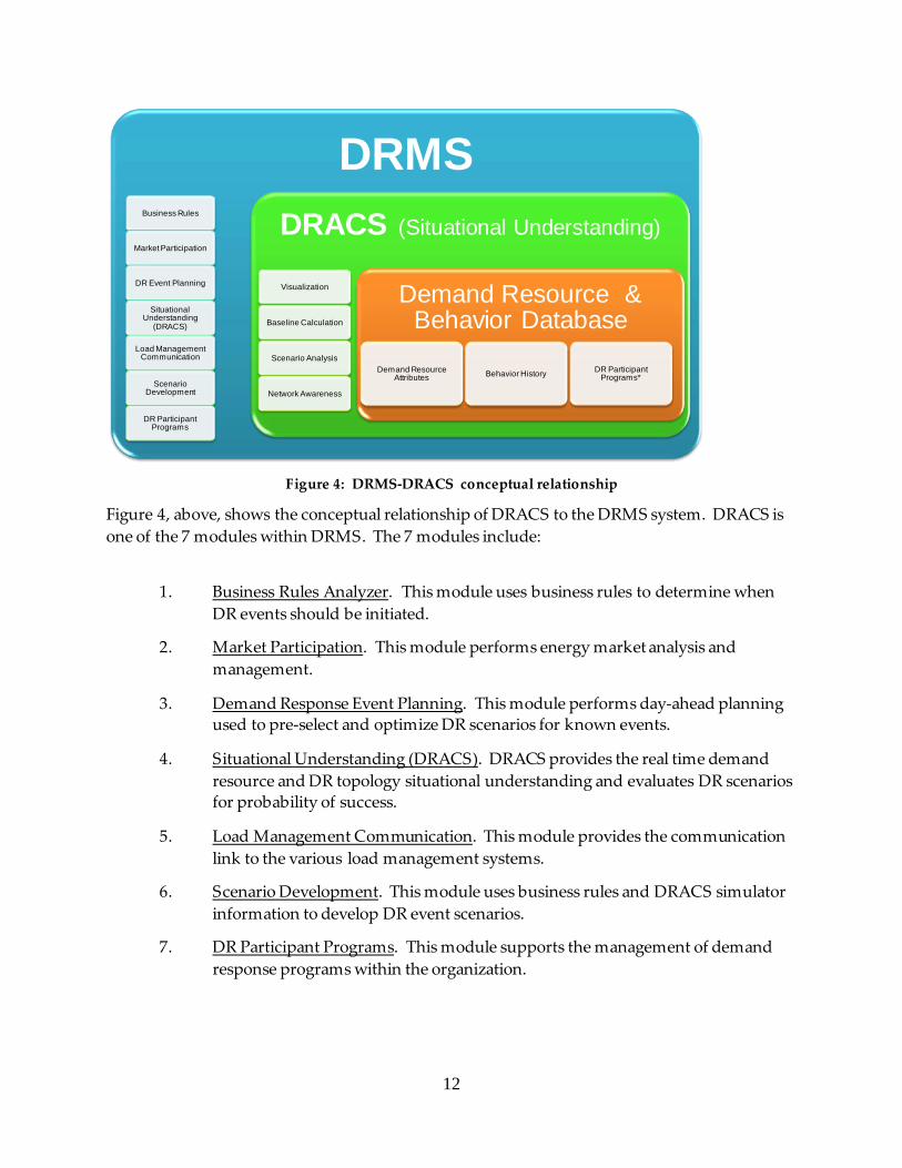
Figure 4, above, shows the conceptual relationship of DRACS to the DRMS system. DRACS is one of the 7 modules within DRMS. The 7 modules include:

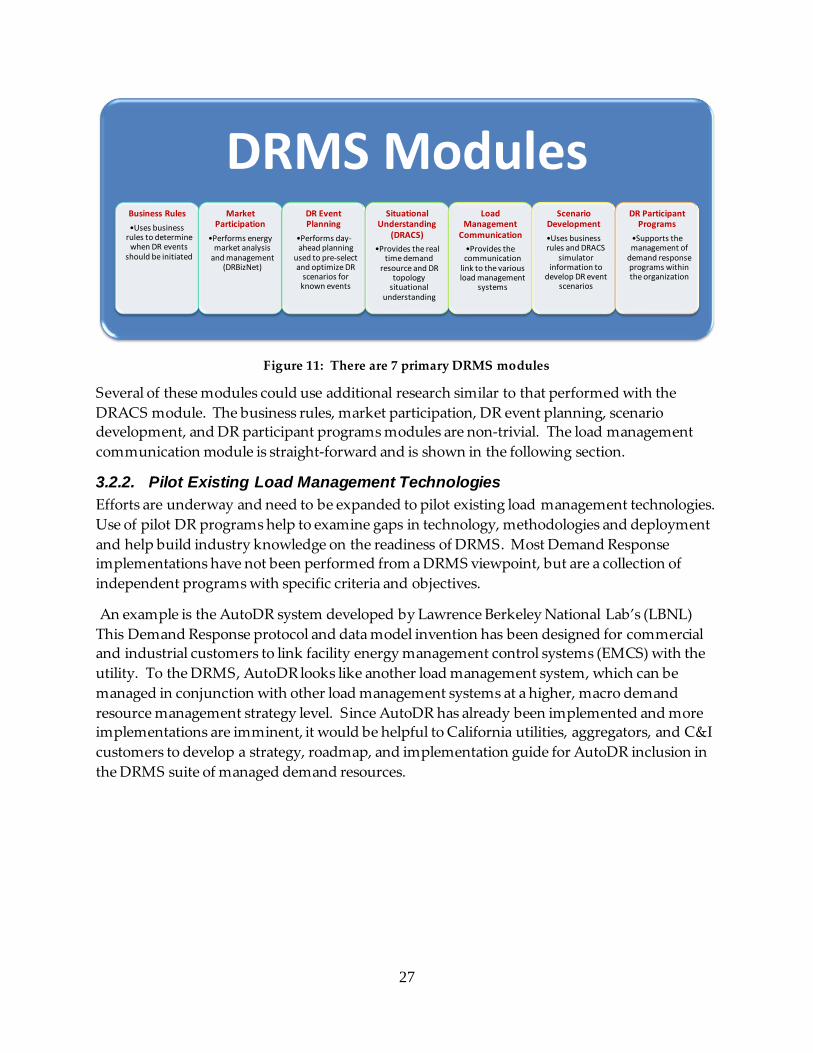
1. Business Rules Analyzer. This module uses business rules to determine when DR events should be initiated.

2. Market Participation. This module performs energy market analysis and management.

3. Demand Response Event Planning. This module performs day-ahead planning used to pre-select and optimize DR scenarios for known events.

4. Situational Understanding (DRACS). DRACS provides the real time demand resource and DR topology situational understanding and evaluates DR scenarios for probability of success.

5. Load Management Communication. This module provides the communication link to the various load management systems.

6. Scenario Development. This module uses business rules and DRACS simulator information to develop DR event scenarios.

7. DR Participant Programs. This module supports the management of demand response programs within the organization.

12

2.2. DRACS Visualization

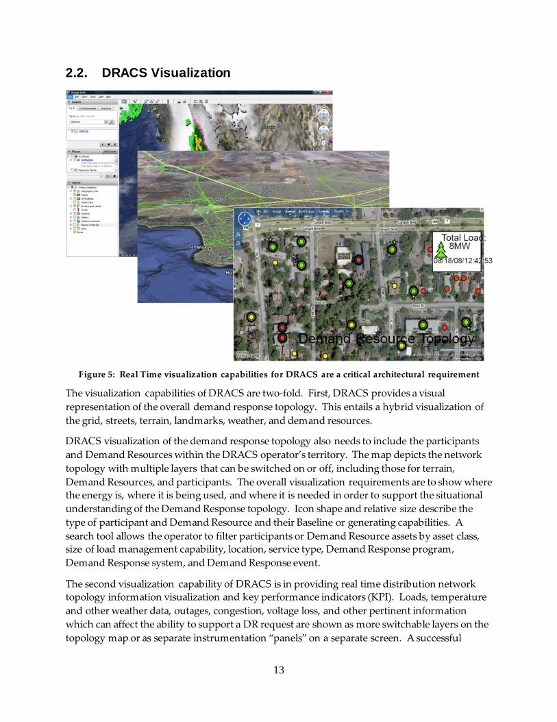
Figure 5: Real Time visualization capabilities for DRACS are a critical architectural requirement

The visualization capabilities of DRACS are two-fold. First, DRACS provides a visual representation of the overall demand response topology. This entails a hybrid visualization of the grid, streets, terrain, landmarks, weather, and demand resources.

DRACS visualization of the demand response topology also needs to include the participants and Demand Resources within the DRACS operator’s territory. The map depicts the network topology with multiple layers that can be switched on or off, including those for terrain, Demand Resources, and participants. The overall visualization requirements are to show where the energy is, where it is being used, and where it is needed in order to support the situational understanding of the Demand Response topology. Icon shape and relative size describe the type of participant and Demand Resource and their Baseline or generating capabilities. A search tool allows the operator to filter participants or Demand Resource assets by asset class, size of load management capability, location, service type, Demand Response program, Demand Response system, and Demand Response event.

The second visualization capability of DRACS is in providing real time distribution network topology information visualization and key performance indicators (KPI). Loads, temperature and other weather data, outages, congestion, voltage loss, and other pertinent information which can affect the ability to support a DR request are shown as more switchable layers on the topology map or as separate instrumentation “panels” on a separate screen. A successful

13

DRACS visualization tool merges the demand response topology and the pertinent real time data.

2.3. DRACS Scenario Analysis

STEP 1: Receive Scenario from DRMS with desired confidence level

STEP 2: Calculate necessary statistical sample size of Scenario Demand Resources

STEP 3: Calculate Expected Load Response mean and standard deviation for the Demand Resource sample (Baseline – historical response)

STEP 4: Multiply mean by total number of Scenario Demand Resources for expected Load Response

STEP 5: Calculate confidence interval for total Load Response

Figure 6: DRACS computes confidence intervals using statistical methodologies in evaluating

scenarios

One of the primary objectives of the DRACS operational system is to provide scenario confidence intervals for meeting DR event requirements in real time. Figure 6 shows the steps for creating Baseline Confidence Intervals for evaluating Demand Response scenarios. DRACS receives a scenario, population total, and expected Confidence Level from other modules within the DRMS. DRACS determines the statistically-significant sample size. Next it calculates or retrieves Baseline information for the sample set and calculates the expected Load Response based on historical or empirical data. The expected Load Response calculation is the “secret sauce” and the reason DRACS requires a true “situational understanding” of the Demand Response landscape. It will use historical data, current electrical network status, weather, social response algorithms, communication loss and latencies, and any number of other proprietary algorithms to accurately predict the expected Load Response for the scenario. DRACS uses all this information to calculate the expected Load Response mean and standard deviations. The final step returns the total expected Load Response and Confidence Interval to the requesting module in DRMS. This may also include metering guidance (frequency of readings, locations, etc.) to verify the required load response.

14

2.4. DERs and Demand Resources 2.4.1. Nomenclature confusion with DERs and Demand Resources One of the revealing aspects of the DRACS project analysis was observing simple nomenclature conflicts. The team settled on the North American Energy Standards Board’s (NAESB) terminology, not because it was the best or most accepted, but because it was published and relatively defensible. Unfortunately, even with this approach, there is still confusion. According to NAESB, the following definitions apply:

• Demand Resource. A Load or aggregation of Loads capable of measurably and verifiably providing Demand Response.

• Demand Response. A temporary change in electricity consumption by a Demand Resource in response to market or reliability conditions.

Our interpretation of Distributed Energy Resources (DERs) in the NAESB nomenclature is that Demand Resources are the opposite of DERs, where DERs provide energy generation capabilities (dispatchable renewable energy resources, small generators, stored energy) and Demand Resources provide load reduction capabilities. Clearly, this is not everyone’s understanding of DERs, where many feel that Demand Resources and Distributed Generation (DG) devices are different forms of DERs. But, for the purposes of the following discussions, we consider DERs as dispatchable supply resources (electricity generators) and Demand Resources as dispatchable loads.

2.4.2. Managing DERs and Demand Resources with the Same DRMS System One of the interesting findings from the DRACS project is that all Demand Resources and Supply Resources (DERs) may be managed within the same system and set of applications, regardless of what you call them.

Curtail LoadsDispatch DER

Electricity Balance

Supply Demand

Increase Price Curtail DERDispatch Loads

Decrease Price

Figure 7: Electricity balance may be controlled by price or direct control signals

As depicted in Figure 5, above, electricity balance of supply and demand may be achieved through price or direct control signals. Most Demand Response discussions focus around the

15

load management side of the equation, and the supply side is either ignored or is considered a different problem, set of systems, and set of applications. This is not at all accurate, and when considering whether to increase or decrease demand, business rules, market conditions, or other constraints (such as weather, grid conditions, societal benefits, etc.) may better support the exact opposite – the decrease or increase of supply.

The concept of using a single set of systems and applications to manage both Demand Resources and DERs is both sound and practical. If all dispatchable resources are managed through the same systems, the likelihood of generating device and load device systems counteracting one another is eliminated. Perhaps even more important is the fact that as these systems mature and historical behavior patterns emerge, energy managers and providers can “learn” from that history and develop optimized approaches for energy balancing situations over time.

The mix of DER and Demand Resource device management under one roof allows 6 different means for balancing the energy supply and demand; 2 pricing mechanisms and 4 direct control mechanisms:

1. Decrease Price. A reduction in price will have the effect of increasing demand and decreasing supply. Energy consumers will want to buy more electricity at lower prices. Energy suppliers will have less incentive to sell at the lower prices.

2. Increase Price. An increase in price will have the effect of decreasing demand and increasing supply. Energy consumers will want to buy less electricity at higher prices. Energy suppliers will have more incentive to sell at the higher prices.

3. Curtail Loads. A direct load curtailment signal will decrease the electricity demand. This is the most common way people think about demand response. It is direct controls to demand resources requesting/demanding energy usage reduction.

4. Curtail DERs. A direct curtailment of DERs will decrease electricity supply. In the event there is too much supply, DERs may be signaled to stop feeding supply into the grid.

5. Dispatch Loads. A direct load dispatch signal will increase demand. This is particularly useful in situations where renewable resources such as Photo-Voltaic (PV) or Wind generators are present and increased loads are needed to optimize their usage.

6. Dispatch DERs. A direct DER dispatch signal will increase supply. In the event of traditional bulk generation losses or shortfalls, direct signals may be sent to dispatch DERs to provide additional electricity supply to the grid.

2.5. Active versus Passive Demand Response Management One of the early debates of the DRACS project was whether the system should perform a handshake with Demand Resources when initiating a Demand Response event. This was a highly debated topic, and after much discussion, the team with help from California utility partners agreed that a passive system made the most sense.

16

With the vast number of demand resources expected to enter the marketplace (with large quantities of demand resource consumer device sales at retail stores a distinct possibility), and with the expectation that bi-directional communication may occur between the DRMS and some of the devices out in the field, we think that in the nearer term such systems are likely to first move through a passive rather than an active management phase. It is also unlikely initially that a 100% accurate list of devices, their capabilities, baselines, and their addresses will exist when DR events are kicked off. To date the implementation of real-time feedback of customer loads from a large number of smart meters is not supported by current technology.

Finally, past behavioral information will certainly help in predicting DR event responses, but there are many variables that will induce uncertainty into the response predictions. Therefore, it makes sense to have a DRMS system that sends DR commands, then using the DRACS module, passively monitors the system on how it responds, at least for residential customers (with potentially millions of demand resources and small per unit load reduction capabilities). The DRMS should not send commands, wait for responses from all the devices, then react based on those responses. There are simply too many devices and too many communications and human behavior issues that will make this level of handshaking overly complex and potentially error-ridden in the beginning. Instead, the DRMS should observe the system’s reaction to the DR event commands and fine tune and send additional signals based on actual response.

The exception to this line of thinking is where large consumption/supply changes may occur, such as C&I customers or an energy service provider/aggregator. In instances such as these, it is logical and practical to have the full handshake and tightly coordinated approach to the DR event in order to avoid over or under-shooting DR event needs by large amounts. AutoDR is a likely candidate technology to utilize in this situation, and can be incorporated into the overall DRMS system and event strategy as one of potentially several load management systems it oversees.

2.6. DRACS Scenario Analyzer/Simulator 2.6.1. Simulator Operation Modes A key component of DRACS is the simulation engine. By clarifying the role of this component, we provide designers insight into the construction of the engine. The “simulator” within DRACS performs scenario analysis and provides design simulation capabilities. The scenario analysis function in DRACS is a “run-time” operational feature responsible for evaluating DR scenarios against DR events in real time. It is responsible for analyzing requests for blocks of energy, capacity, reserves, or ancillary services and providing a predictive confidence level for success in meeting the requested DR event with the set of available mechanisms and real-time state.

There is also an “off-line” simulation feature that evaluates expected DR penetration, scope of dispatch strategies, range of behaviors, etc. in varied scenarios (including worst-case). Here the goal is to determine what strategies need to be designed and made available within the system prior to the actual DR event. This simulation feature is useful when there are planned DR events, and multiple scenario responses may be simulated and evaluated. The simulator

17

functionality overlaps with the scenario analysis run-time module. The run-time module must handle a specific case, and thus needs more accurate current event information. The off-line simulator exercises a broad set of response scenarios and hence some of the inputs may be generalized and the event conditions are predicted, rather than actual. Both the “off-line” and “run-time” simulator have the same sub-modules and operate effectively in the same manner, but their functions are different in that the “run-time” simulator evaluates one scenario at a time in real time, and the “off-line” simulator evaluates multiple scenarios and “scores” them for their ability to meet a future DR event’s requirements.

To summarize:

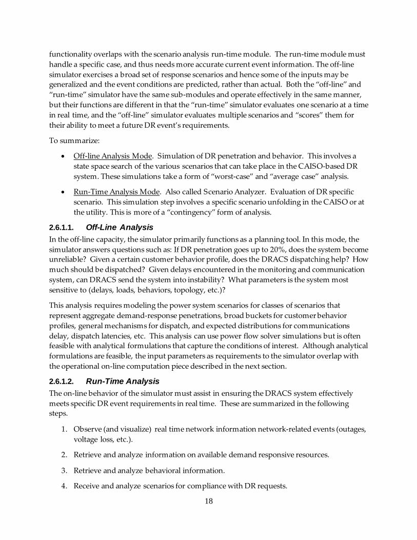
• Off-line Analysis Mode. Simulation of DR penetration and behavior. This involves a state space search of the various scenarios that can take place in the CAISO-based DR system. These simulations take a form of “worst-case” and “average case” analysis.

• Run-Time Analysis Mode. Also called Scenario Analyzer. Evaluation of DR specific scenario. This simulation step involves a specific scenario unfolding in the CAISO or at the utility. This is more of a “contingency” form of analysis.

2.6.1.1. Off-Line Analysis In the off-line capacity, the simulator primarily functions as a planning tool. In this mode, the simulator answers questions such as: If DR penetration goes up to 20%, does the system become unreliable? Given a certain customer behavior profile, does the DRACS dispatching help? How much should be dispatched? Given delays encountered in the monitoring and communication system, can DRACS send the system into instability? What parameters is the system most sensitive to (delays, loads, behaviors, topology, etc.)?

This analysis requires modeling the power system scenarios for classes of scenarios that represent aggregate demand-response penetrations, broad buckets for customer behavior profiles, general mechanisms for dispatch, and expected distributions for communications delay, dispatch latencies, etc. This analysis can use power flow solver simulations but is often feasible with analytical formulations that capture the conditions of interest. Although analytical formulations are feasible, the input parameters as requirements to the simulator overlap with the operational on-line computation piece described in the next section.

2.6.1.2. Run-Time Analysis The on-line behavior of the simulator must assist in ensuring the DRACS system effectively meets specific DR event requirements in real time. These are summarized in the following steps.

1. Observe (and visualize) real time network information network-related events (outages, voltage loss, etc.).

2. Retrieve and analyze information on available demand responsive resources.

3. Retrieve and analyze behavioral information.

4. Receive and analyze scenarios for compliance with DR requests.

18

The simulator’s operation in real-time takes data collected and stored in the first three steps listed above (supported by the overall DRACS system) and gives the results and guidance for step 4.

2.6.2. Simulator Functional Components Figure 6, below, shows the DRACS Scenario Analyzer/Simulator.

Figure 8: DRACS Architecture Components

The conceptual framework within the simulator is illustrated in the figure below:

C2 Latency Estimates

Dispatch Rules Engine

Response Estimates

Priority Assignment

Topology Customer Behavior

Weather, CZ, TOD

SCADA and State-Estimates

Power Flow Estimates

Impact Estimates

Operator Input and Guidance Resource Dispatch Candidates

Figure 9: Operational Flow in Simulator Components

The operational flow of the run-time simulator function is illustrated by the flow of data from the databases through the solver and into an operator feedback and control tool.

19

The DRMS generates scenarios for managing each DR event. These scenarios are built based on business rules and from a collection of Demand Resources in the Demand Resource Attribute and Behavior database that meets both the business rules and DR event requirements. DRACS receives a scenario from the DRMS. The simulator’s on-line analysis function evaluates the scenario against the collection of Demand Resources Baseline estimates and previous behavior, current electrical network events, and topology communication and social response algorithms and calculates the likelihood of success in meeting the DR event objectives. DRACS compares against “Baseline” values which are estimates of the electricity that would have been consumed by a Demand Resource in the absence of a Demand Response Event. Depending on the type of Demand Response product or service (one of energy, capacity, reserve, or regulation service), baseline calculations may be performed in real-time or after-the-fact. The baseline is compared to the desired metered electricity consumption during the Demand Response Event to determine the Demand Reduction Value. There are three Types of Baseline Models:

1. Baseline Type 1 (Interval Metered) - A Baseline model based on a Demand Resource’s historical interval meter data which may also include but is not limited to other variables such as weather and calendar data.

2. Baseline Type 2 (Non-interval Metered) - A Baseline model that uses statistical sampling to estimate the electricity consumption of an Aggregated Demand Resource where interval metering is not available on the entire population.

3. Behind-The-Meter Generation - A performance evaluation methodology, used when a generation asset is located behind the Demand Resource’s revenue meter, in which the Demand Reduction Value is based on the output of the generation asset. Distributed generation resources are considered “behind-the-meter” generators, such as combined heat and power (CHP) systems, wind turbines, and photovoltaic generators that generate electricity on site.

The DRACS simulator uses baseline values and estimates of the dispatched load or available ancillary service to provide statistical confidence levels for the DRMS system to go forward with the implementation of the control decisions.

2.6.2.1. Simulator Components The simulator sub-modules are shown in Figure 9: Operational Flow in Simulator . In addition to those sub-modules, there are support components that ingest or convert between data representations to support the operations of other sub-modules. We list those as well – a complete list of sub-modules in each of its two modes of operation is as follows:

1. Offline analysis mode

a. Input parameter ingest engine

b. Topology mapping module

c. Power flow solver

20

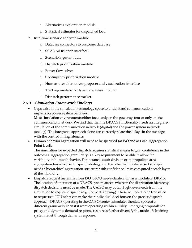
d. Alternatives exploration module

e. Statistical estimator for dispatched load

2. Run-time scenario analyzer module

a. Database connectors to customer database

b. SCADA/Historian interface

c. Scenario ingest module

d. Dispatch prioritization module

e. Power flow solver

f. Contingency prioritization module

g. Human-user alternatives proposer and visualization interface

h. Tracking module for dynamic state-estimation

i. Dispatch performance tracker

2.6.3. Simulation Framework Findings • Gaps exist in the simulation technology space to understand communications

impacts on power system behavior. Most simulation environments either focus only on the power system or only on the communication network. We find that that the DRACS functionality needs an integrated simulation of the communication network (digital) and the power system network (analog). The integrated approach alone can correctly relate the delays in the message with the control timing latencies.

• Human behavior aggregation will need to be specified (at ISO and at Load Aggregation Point level). The simulation for expected dispatch requires statistical means to gain confidence in the outcomes. Aggregation granularity is a key requirement to be able to allow for variability in human behavior. For instance, a sub-division or metropolitan area aggregation has a focused dispatch strategy. On the other hand a dispersed strategy needs a hierarchical aggregation structure with confidence limits computed at each layer of the hierarchy.

• Dispatch request hierarchy from ISO to IOU needs clarification as a module in DRMS. The location of operation of a DRACS system affects where in the distribution hierarchy dispatch decisions must be made. The CAISO may obtain high-level needs from the simulation to request dispatch (e.g., for peak shaving). These will need to be translated to requests to IOU’s that can make their individual decisions on the precise dispatch approach. DRACS operating in the CAISO context simulates the state space at a different granularity than if it were operating within a utility. Emerging proposals for proxy and dynamic demand response resources further diversify the mode of obtaining system relief through demand response.

21

• Statistical aggregation approach are effective but estimates (for operators) will need to be validated with monitoring signals during operation There are emerging recommendations to monitor the system for Demand Resources status. With statistical estimation, although the appropriate levels of confidence limits may be achieved, the reliability of the power system will require sampling of the set of demand resources. Thus there is an aggregation of the probabilistic estimate of dispatch, and an estimate of the actual system status by sampling. More pervasive sampling, possibly integrated with emerging metering infrastructures will fill any confidence gaps. The confidence gaps in the interim must be maintained within the margin of tolerance for reliability.

• Delay vs. Control tradeoff differs for different technology mix for dispatch. Integrating technology alternatives in one bag for dispatch will need a lot of simulation to get confidence. Current simulations abstract load behavior. These will need to be refined according to the technologies dispatched. The delays in obtaining the response (to, e.g., Time-Of-Day pricing related thermostat settings vs. critical peak price signals) affect the stability of the system. The dispatch strategy must simulate the response time based on the technology dispatched.

2.6.4. Simulator Framework Case-Study Example

Controllable load can in part replace generation for frequency regulation and spinning reserve. How this is done depends on the time scales available for control. Control of frequency in an emergency, to prevent under frequency failures for example, requires action in seconds to minutes. Load acting as spinning reserve has minutes to act. The potential for dynamic control can be understood with a very simple model, which we evaluate by simulation of a detailed model of a centralized control process operating on the IEEE 118 bus test system. The details of this case-study may be found in the results of Task 4 (see Section 1.2.4). This scenario uses the IEEE 118 bus test case. There are 34 generators, each modeled with uniform dynamic parameters. To emphasize the role of the load control in damping frequency oscillations, the control parameters of the generators are set to give the system an under-damped response to a step change in load. For this experiment, there is a 30% reduction in the electrical load at t=1 second. Figure 10 (a) shows the response of the 34 generating units when active load control is not used; the under-damped response is obvious in the large, initial swings between 61 and 58.5 Hertz. Figure 10 (b) shows the improved response for the same experiment but with active control of the loads; superimposed on the frequency plot is the load reduction effected by the control center. In this case, the control center is notified of every 0.2 Hz change in frequency at the terminals of the generators. These measurements arrive via the communication network, and, upon receipt, the control center uses the average value of its frequency measurements to determine the quantity of demand-responsive load to be dispatched (shed). The adjusted load level is then transmitted to the load busses via the communication network, each bus acting on the request when it is received.

22

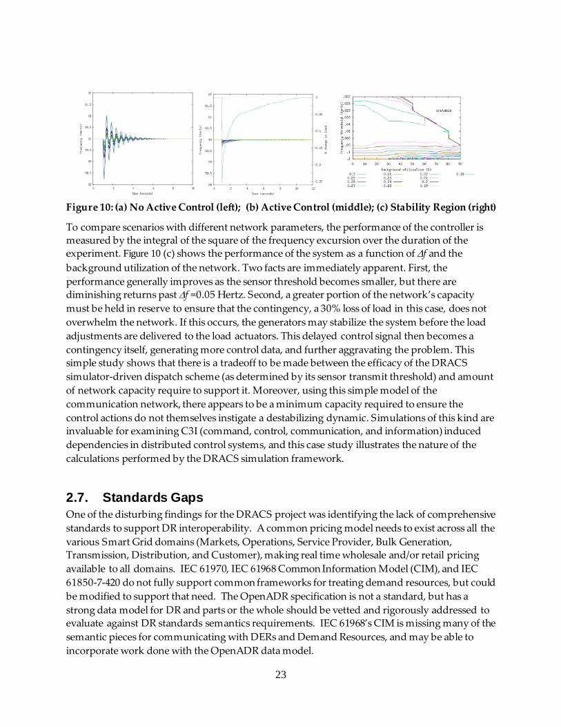
Figure 10: (a) No Active Control (left); (b) Active Control (middle); (c) Stability Region (right)

To compare scenarios with different network parameters, the performance of the controller is measured by the integral of the square of the frequency excursion over the duration of the experiment. Figure 10 (c) shows the performance of the system as a function of ∆f and the background utilization of the network. Two facts are immediately apparent. First, the performance generally improves as the sensor threshold becomes smaller, but there are diminishing returns past ∆f =0.05 Hertz. Second, a greater portion of the network’s capacity must be held in reserve to ensure that the contingency, a 30% loss of load in this case, does not overwhelm the network. If this occurs, the generators may stabilize the system before the load adjustments are delivered to the load actuators. This delayed control signal then becomes a contingency itself, generating more control data, and further aggravating the problem. This simple study shows that there is a tradeoff to be made between the efficacy of the DRACS simulator-driven dispatch scheme (as determined by its sensor transmit threshold) and amount of network capacity require to support it. Moreover, using this simple model of the communication network, there appears to be a minimum capacity required to ensure the control actions do not themselves instigate a destabilizing dynamic. Simulations of this kind are invaluable for examining C3I (command, control, communication, and information) induced dependencies in distributed control systems, and this case study illustrates the nature of the calculations performed by the DRACS simulation framework.

2.7. Standards Gaps One of the disturbing findings for the DRACS project was identifying the lack of comprehensive standards to support DR interoperability. A common pricing model needs to exist across all the various Smart Grid domains (Markets, Operations, Service Provider, Bulk Generation, Transmission, Distribution, and Customer), making real time wholesale and/or retail pricing available to all domains. IEC 61970, IEC 61968 Common Information Model (CIM), and IEC 61850-7-420 do not fully support common frameworks for treating demand resources, but could be modified to support that need. The OpenADR specification is not a standard, but has a strong data model for DR and parts or the whole should be vetted and rigorously addressed to evaluate against DR standards semantics requirements. IEC 61968’s CIM is missing many of the semantic pieces for communicating with DERs and Demand Resources, and may be able to incorporate work done with the OpenADR data model.

23

2.8. Human Behavior and Plug-n-Play Human behavior is the most unpredictable aspect of DR event scenario generation. It will take time for models of human behavior and anticipated reaction to DR events to mature. A statistical representation will need to be incorporated and refined over time (due to changing economic and social environment conditions) in a realistic DRMS. The DRMS and its operator will need to be nimble, observing grid activities and DR responses, and be prepared to “fine tune” DR signals and commands until the grid conditions meet acceptable tolerance levels.

Another aspect of human behavior here that influences these systems is the current inclinations in society and demographics (as different from consumption patterns which utilities handle well). Factors such as peer pressure and vaguely defined social responsiveness are likely to be enablers of DR adoption, and the potential rush of DERs and Demand Resources into the American home will probably have a much more dramatic effect on the level of DR event support than anticipated – especially once DERs and Demand Resources are available in retail stores as plug-n-play consumer devices, and they automatically respond to event signals with little or no human interaction.

Plug-n-play interoperability will be a necessity once DERs and Demand Resources become purchases consumers can make easily. How this will be done, whether the devices will auto-register themselves in some “global device registry”, or whether the utility/ISO even needs to be aware of a particular device’s presence on the grid has not been decided. It is not even clear where the lines of demarcation between the consumer and the grid are. At what point does the consumer electronics industry assume control and the electric power industry relinquish control to the consumer? Does it end at the meter or premise gateway? Or, can the utility/service provider/ISO enter the customer premise and talk directly to the devices? Or, is there some hybrid solution where some devices are directly controlled by an outside entity or service provider, but others are managed only by the consumer himself? It is a challenge that is certainly solvable, but it has profound implications for how DRACS and the DRMS manage DERs and Demand Resources (and how many).

24

3.0 Summary, Conclusions, and Recommendations In comparing a utility operation with military mission, military organizational requirements call for tight coordination of multiple command structures controlling individual resources and assets integrated in a coordinated action to achieve an objective in support of a mission. Similarity with a utility organization is the multiplicity of individual resources and assets controlled by individual departments. Unlike military organizations, a utility’s mission is singular (lowest cost electricity at highest reliability) and non-changing although objectives are evolving and changing with the advent of new Smart Grid technologies such as

• integration of distributed generation especially renewables

• implementation of smart metering

• providing customer access to energy usage

• integration of advanced grid control devices

• integration of demand response resources

• serving plug-in electric vehicles (PEVs)

What constitutes C3I in the military directly maps to C2I in the utility world dropping “Command” functionality which is not applicable. This project has developed a Control Communication and Information (C2I ) system architecture that provides utilities the ability to identify, organize, analyze, forecast and execute demand response resources.

Classical military C3I systems have evolved that integrate real time data sources with behavior analysis and decision making toolsets. This capability is just now appearing in the utility industry. With real time up-to-date information available from all customers and across distribution grid and distributed resources, utilities can now use C2I methodologies to develop operational strategies that are built upon high performance computational platforms.

The findings identified in the previous sections lead to the conclusion that further research is needed around DRACS and the DRMS. Demand Response is still quite immature. This is evident in the various different ways that the California utility companies are approaching Demand Response deployments. Like many other Smart Grid technologies, California is out in the lead with Demand Response technologies. There is obviously risk associated with being the early adopter and trailblazer, but also opportunities to lead the industry, set a precedent, and help find solutions that not only work well in California, but also in the rest of the US and beyond. This risk can be mitigated by using layered software technology and loose coupling, ensuring firmware is remote-upgradeable, and by objectively reviewing the DR landscape, standards development requirements and timelines, regulatory and policy inertia, and consumer products plans around Demand Resources and DERs. In fact, a comprehensive risk analysis may suggest that California closely track NIST Interoperability

25

Standards adoption. Nevertheless, there are unique regulatory demands and critical peak power conditions experienced by California grid participants that require aggressive action. There is a critical need to perform additional technology, policy, risk, security, process, and peer analyses before DR strategies and systems are committed. California should invest in these types of studies and work to ensure that the large IOU utilities’ DR systems can interoperate with each other and the CAISO for the overall benefit of the utilities and grid partners, and consumers.

3.1. DRACS Follow-on Recommendations Research is needed in the following areas that will result in technologies that are embodied in C2I offerings:

• Development of a full prototype simulator for creating and evaluating DR scenarios

• Automatic device registry mechanism for demand resources

• Demand Resource behavior models for each customer class and device class

• Input into industry groups such at Open Smart Grid AMI Enterprise Working Group. (See AMI Ent Use Cases 1.0 http://osgug.ucaiug.org/utilityami/AMIENT/Shared%20Documents/Forms/AllItems.aspx?RootFolder=%2futilityami%2fAMIENT%2fShared%20Documents%2fUse%20Cases&FolderCTID=&View=%7bAE210767%2d1957%2d42A0%2dA6B4%2d46E383ED6114%7d )

• Support industry standardization of Demand Response business processes at NAESB. (See NAESB Demand Side Management and Energy Efficiency Working Group http://www.naesb.org/dsm-ee.asp )

3.2. DRMS Research Recommendations 3.2.1. DRMS Module Elaboration There are many questions to answer about what the optimal DRMS system should look like, the modules necessary, requirements and reference architecture for each module, the internal and external interfaces, and the system information flow. Is it a separate Enterprise system? Is it multiple systems? Or, is it part of the Distribution Management System (DMS)?

The EnerNex team needed a mid-level understanding of the overall DRMS system in order to properly carve out and address the requirements and reference architecture for DRACS. We spent the first two months of the DRACS project working internally and then with SDGE and Lockheed Martin system engineers to establish and agree upon the DRACS/DRMS relationship discussed in section 2.1.3. The result of this collaborative effort was the identification of seven (7) primary modules and a high level functional description of each.

26

DRMS ModulesBusiness Rules•Uses business

rules to determine when DR events

should be initiated

Market Participation

•Performs energy market analysis

and management (DRBizNet)

DR Event Planning

•Performs day-ahead planning

used to pre-select and optimize DR

scenarios for known events

Situational Understanding

(DRACS)•Provides the real

time demand resource and DR

topology situational

understanding

Load Management

Communication•Provides the communication

link to the various load management

systems

Scenario Development•Uses business rules and DRACS

simulator information to

develop DR event scenarios

DR Participant Programs

•Supports the management of

demand response programs within the organization

Figure 11: There are 7 primary DRMS modules

Several of these modules could use additional research similar to that performed with the DRACS module. The business rules, market participation, DR event planning, scenario development, and DR participant programs modules are non-trivial. The load management communication module is straight-forward and is shown in the following section.

3.2.2. Pilot Existing Load Management Technologies Efforts are underway and need to be expanded to pilot existing load management technologies. Use of pilot DR programs help to examine gaps in technology, methodologies and deployment and help build industry knowledge on the readiness of DRMS. Most Demand Response implementations have not been performed from a DRMS viewpoint, but are a collection of independent programs with specific criteria and objectives.

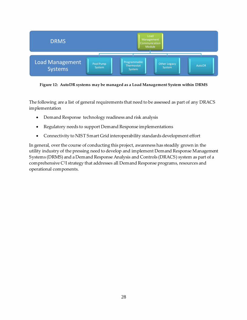
An example is the AutoDR system developed by Lawrence Berkeley National Lab’s (LBNL) This Demand Response protocol and data model invention has been designed for commercial and industrial customers to link facility energy management control systems (EMCS) with the utility. To the DRMS, AutoDR looks like another load management system, which can be managed in conjunction with other load management systems at a higher, macro demand resource management strategy level. Since AutoDR has already been implemented and more implementations are imminent, it would be helpful to California utilities, aggregators, and C&I customers to develop a strategy, roadmap, and implementation guide for AutoDR inclusion in the DRMS suite of managed demand resources.

27

Load Management Systems

DRMSLoad

Management Communication

Module

Pool Pump System

Programmable Thermostat

System

Other Legacy System AutoDR

Figure 12: AutoDR systems may be managed as a Load Management System within DRMS

The following are a list of general requirements that need to be assessed as part of any DRACS implementation

• Demand Response technology readiness and risk analysis

• Regulatory needs to support Demand Response implementations

• Connectivity to NIST Smart Grid interoperability standards development effort

In general, over the course of conducting this project, awareness has steadily grown in the utility industry of the pressing need to develop and implement Demand Response Management Systems (DRMS) and a Demand Response Analysis and Controls (DRACS) system as part of a comprehensive C2I strategy that addresses all Demand Response programs, resources and operational components.

28

APPENDIX O Appendix O: Appendix 8: Decision Support for Demand Response Triggers: Methodology Development and Proof of Concept Demonstration

CHAPTER 1: Introduction This report describes a project conceptualized to address the prevalent disconnect between retail and wholesale electricity markets that persists in regions that have undergone restructuring of the electric power industry, including California. A decision support tool is needed to inform energy retailers of wholesale settlement costs that demand response can help avoid. The report describes an innovative methodology for triggering demand response to capture value for wholesale market participants, embodied in a Demand Response Triggers Decision Support tool. Such a tool could be used in operational timeframes to establish a financial link between retail incentives for demand response and actual wholesale market conditions.

1.1 Background and Foundation for the Work Since the early 1980s, EPRI has managed collaborative RD&D programs to support demand-side integration, including the electric power industry’s migration towards load management and demand-side response. Despite the growing recognition of the importance of demand-side response, widespread implementation has yet to be realized, including in restructured electricity markets.

Enabling technology initiatives exist to target needed metering, communications, and control infrastructure for measuring and actuating demand response. Moreover, dynamic pricing initiatives address retail tariff structures that encourage demand response through time-varying prices. The California Energy Commission (CEC) and the California Public Utility Commission (CPUC) are targeting Critical Peak Pricing (CPP), Real-time Pricing (RTP), and Time of Use (TOU) as default tariffs for California end-use customers. These tariff structures are envisioned to provide a financial mechanism to incentivize demand response according to dynamic triggers, price signals, or pre-designated hours of the day. Careful design of such dynamic triggers or information signals is critical in connecting financial consequences of wholesale electricity markets with retail incentives for demand response. Nevertheless, a prevalent disconnect exists between retail and wholesale electricity markets. This situation is particularly evident in restructured regions, where wholesale electricity costs vary with wholesale market and grid conditions, yet retail customers are disconnected from wholesale conditions and lack incentive to respond in a timely manner.

Furthermore, present implementations of demand response (DR) are limited. Under status quo as depicted in Figure 1, demand response is predominantly triggered based on pre-set physical system conditions (e.g., emergency stage alerts, temperature, weather, etc.) or pre-set market-driven economic conditions (e.g., spot energy price, heat rate, etc.). In contrast, the project described in this report investigates a combination of both wholesale market and system conditions for triggering demand response, which together determine overall wholesale costs. That is, the project investigates a broader scope of costs by analyzing various components that comprise costs (e.g., prices and quantities from a series of markets). In contrast to the status quo, project findings have the potential of supporting both dynamic pricing and traditional demand response programs by providing a tool for energy retailers to coordinate the triggering of demand response considering an array of wholesale costs.

7

Previous work in [1] suggests enhanced benefits to be captured from applying real-time information technology tools to dispatch resources based on latest power system and market conditions. It follows that benefits can also be derived from triggering demand-side resources based on latest information available on the day of operations. Furthermore, [2] suggests demand response may be applied to avoid premiums in wholesale costs during times of supply shortfall in competitive electricity markets. This report details execution of a plan to investigate the suggested financial connection between demand response and wholesale market costs, and to investigate supporting information technology that enables capture of avoided costs. By enhancing the energy retailers’ understanding of wholesale cost impacts of demand response and how to capture wholesale cost savings, the project is designed to reveal benefits that can be passed onto end-use customers to help incentivize demand response.

Figure 1: Status quo for triggering demand response contrasted with proposed research investigation

1.2 Project Objectives The project seeks to devise and demonstrate a method of triggering demand response that captures value for market participants that schedule load. To do so, EPRI envisioned bringing together a collaborative project team from retail and wholesale organizations across the electric power industry to define a decision support tool for informing energy retailers of various wholesale settlement costs that demand response can help avoid. Such a tool would be used in operational timeframes to provide a financial link between retail incentives for demand response and actual wholesale market conditions.

The project addressed these objectives by investigating the following underlying research questions:

End-Use Customer

CAISO

Energy Retailer

Emergency or Economic Signal • Reduction Request • Emergency Stage Alert • Wholesale Price

Wholesale Market and System Conditions • Wholesale Costs • Wholesale Prices • Metered Quantities • System Congestion, Reserves, etc.

CAISO

DR Trigger • Dispatch/Notification based on Stage Alert,

Weather, Heat Rate or Wholesale Spot Price • Ad-hoc Retail Price Signal

Demand Response Resource

Actuation Method • Manual Switching • Control Signal • Retail Price Signal

Energy Retailer

End-Use Customer

Demand Response Resource

DR Trigger • Dispatch/Notification based on

Wholesale Costs • Retail Price Signal based on Wholesale

Costs

STATUS QUO RESEARCH INVESTIGATION

Actuation Method • Manual Switching • Control Signal • Retail Price Signal

8

• What operational approach to triggering demand response will enable energy retailers to mitigate wholesale market settlement charges?

• What decision support tool will enable energy retailers to create demand response triggers based on impact to wholesale settlement costs?

Overall, the purpose of the project is to develop an operational approach and supporting information technology that will substantially bridge the current disconnect between wholesale and retail electricity markets. The outcome envisioned is a new operational methodology and decision support tool enabling energy retailers to coordinate the triggering of demand response based on impact to wholesale settlement costs.

1.3 Project Funders The project is a joint effort funded by the California Energy Commission’s PIER Program and CIEE, as well as EPRI. Substantial in-kind services were provided by Southern California Edison, Pacific Gas & Electric, the California Independent System Operator, the California Department of Water Resources, and other project participants. The rationale of co-funding the research reported in this document is to leverage the extensive body of work and personnel expertise required for the development of a DR Triggers Decision Support Tool.

1.4 Report Structure Section 1 introduces the background and objective of the project. The project team’s approach to addressing the objectives are structured into tasks described in Section 2. The development of the DR Trigger methodology is captured in Sections 3 and 4. The information technology specification is summarized in Section 5 and potential benefits in Section 6. Section 7 describes the proof of concept development and demonstration. Section 8 identifies the project’s next steps. Section 9 outlines project conclusions.

9

CHAPTER 2: Project Approach 2.1 Cross-Functional Team EPRI assembled a cross-functional group of wholesale market participants, energy retailers, and information technologists to inform stages of the project as appropriate. Engaging the industry experts who possessed targeted expertise and information access was a critical factor to the success of the project. The resulting team of project participants included personnel from the four largest load-serving entities (LSEs) in California and the California Independent System Operator (CAISO). The project approach to engage personnel from both procurement and retail organizations of the LSEs resulted in a team exceptionally well qualified to bridge gaps between wholesale and retail operations. Besides EPRI technical development resources, the principal investigator was assisted by subcontractors with targeted expertise in wholesale settlements.

2.2 Top-Down Approach The project team executed Phase 1 of a two-phased approach for the overall DR Triggers project. Phase I of the project, the subject of this report, was to develop and prove feasibility of the concept. Major project tasks included trigger methodology design, information technology specification, and proof of concept development and demonstration. A future Phase II of the project would focus on implementation and demonstration of the decision support tool specified in Phase I.

A systematic, four-step approach was followed in executing the project to achieve the stated objectives. Major project tasks included:

• DR Trigger Methodology Development

• Information Technology Specification

• Proof-of-Concept Demonstration

• Reporting and Publication

10

Figure 2 depicts the process steps followed in executing the project under three major project stages.

Figure 2: Process followed in the DR Triggers project

In Stage 1, DR Trigger Methodology Development, the project team identified and classified charge codes allocable to loads and relevant to demand response (DR). The team assessed the potential impact of DR and ranked each one by high to low value application of DR. DR impact assessment was performed utilizing aggregated historic settlement data from market participants that schedule load. Charge codes were ranked based the combination of 1) relevance of DR and 2) significance of the charge code on actual settlements charged to market participants that schedule load. Charge code ranking was an essential step for establishing priorities for further investigation in Task 2 of methodologies to reduce the most problematic charges. Prerequisite data and other requirements for estimating the impact of demand response by charge code were also identified, along with concrete examples of the potential impact of DR on settlement charges.

In Stage 2, Information Technology Specification, the team specified and prioritized software requirements based on input from project participants and potential users of the DR Trigger Decision Support tool. Substantial in-kind services were provided by utility personnel to support this task. Requirements were gathered on desired functionality and user interface contents. Sample input data was collected revealing useful data formats. Project participants also prioritized the resulting specified requirements.

In Stage 3, Proof of Concept Demonstration, the project team targeted a limited subset of the specified requirements for proof-of-concept development, testing, and demonstration. The team discussed various scenarios for demonstration. A subset of scenarios was selected to demonstrate value-added capabilities during a live demonstration of the prototyped decision support tool. The demonstration was given at a final project workshop held with project participants and funders at a face-to-face meeting hosted by the Energy Commission in

Stage 1 Stage 2 Stage 3

11

Sacramento. The final project workshop presentation and demonstration were also shared through a live webcast that was open to public participation.

At the conclusion of the final workshop, EPRI led a meeting with the project participants to discuss next steps. The next steps form the basis for a detailed implementation plan being proposed for a subsequent phase of the project. The implementation plan and findings from each task of the project are shared in this report.

2.3 Value Capture for Energy Retailers The project approach emphasizes developing a methodology and tool to support value capture for energy retailers that schedule load and can trigger demand response in day-to-day operations. By focusing on value-add for market participants on the demand-side of electricity markets, the approach has the potential of revealing value at anytime during the year based on latest market conditions.

As market participants positioned between end-use customers and wholesale electricity markets, energy retailers (or their affiliates that schedule load) are well-positioned to facilitate a connection between retail load and wholesale markets. However, these market participants may require tools to augment their decision-making capabilities and to clarify what value can be derived from triggering demand response. The project approach focuses on clarifying the financial impact of triggering demand response and resulting benefits to energy retailers that schedule load in wholesale markets.

By triggering demand response to achieve savings on wholesale electricity market charges (in both ISO and bilateral markets), retail markets become inherently integrated with wholesale markets. Savings discovered at the wholesale level in turn provide a source of retail incentives for demand response. This is unlike traditional demand response programs that require an external source to fund demand response incentive payments. In contrast, the project approach has the potential of revealing persistent strategies for wholesale cost reductions, by identifying market-based financial incentives for demand response. Strategies with such a market connection are applicable on an ongoing 24x7 basis for revealing incentives for demand response. Therefore, the project approach focuses on devising a flexible tool that enables energy retailers to connect retail load to wholesale markets, by clarifying the impact of demand response on wholesale settlement charges.

12

CHAPTER 3: Settlement Charge Code and Data Analyses This section summarizes findings from analyses conducted under Stage 1 of the project. The project commenced with analyses of charge codes and settlement data. The goal was to prioritize charge codes for further investigation.

The charge code and data analyses work followed the process depicted in Figure 3. The process began with identifying the charge codes most sensitive to demand response and information sources required as inputs to their calculations. The analyses focused on charge codes that were in effect prior to the California Market Redesign and Technology Upgrade (MRTU) in April 2009. A mapping was also performed between existing (pre-MRTU) and new charge codes introduced by MRTU that are relevant to DR. The task continued with aggregation of settlement data in order to determine the most significant charge codes based on historical data. The final step of the analyses was to rank charge codes based on sensitivity to demand response and significance on settlements for market participants that schedule load. The next four subsections detail findings from the analyses.

Figure 3: Charge code and data analysis process

3.1 Charge Code Identification and Categorization The project team identified and categorized pre-MRTU and MRTU charge codes relevant to Demand Response. Charge codes can be identified by identification number, name, category grouping, and billable quantity, as illustrated in Figure 4. Pertinent information captured also includes time period the charge code is in effect, status of the charge code (i.e., active or inactive at the time of analyses), and status under MRTU (i.e., charge code to be replaced, retired, or newly introduced with MRTU). Results are summarized in the table in Appendix B-1. The table includes a list of billable quantities that serve as inputs to the calculations of charges per charge code. Results also include a preliminary mapping between existing and new charge code introduced by MRTU that are relevant to demand response. Figure 4 provides a partial listing of charge codes as an example of how they can be identified and categorized. Appendix B-1 provides a full list of charge codes identified and categorized at the time of investigation before the California market transitioned to MRTU.

13

Figure 4: Example table structure for identifying and categorizing charge codes

The charge code identification list also indicates which charge codes are relevant to demand response. Different charge codes are applicable to different resource types. The charge codes relevant to demand response are those allocable to dispatchable participating load and non-participating load, as indicated by an “X” in Figure 4 and in the table under Appendix B-1. A full list of resource types is given below, with the types relevant to demand response shown in italics.

• Generators

• Pump Storage Gen

• Dispatchable participating load

• Non-participating load

• Import

• Dynamic Import

• Export

• INTER-SC Trade

• Metered Subsystem

• Participating Transmission Owner

• UDC

• FTR/CRR

• Transmission Ownership Rights

Column three of the charge code listing captures the outcome of grouping charge codes by category. This column shows the grouping that each charge code falls under. A full list of charge code categories and their associated abbreviated term is shown below.

* MD02 Charge Code

Number

MD02 Charge Code Name Group MD02 Status

MRTU Status Billable Quantity

Dispatchable-Participating Load:

- Pump Storage Load- Single Pump

- Aggregated Pump

Non-Dispatchable / Non-Participating LOAD

Prior Charge Code

Start End

2 Day Ahead Non-Spinning Reserve due SC AS Active Replaced Day Ahead Non Spin Capacity Awarded X 4/1/1998 Open

4 Day Ahead Replacement Reserve due SC AS Active Retired Replacement Reserve Accepted Bid Quantity X 4/1/1998 Open

24Dispatched Replacement Reserve (Bid-In) Capacity

WithholdAS Active Retired Amount of 'bid-in' Replacement Reserve

capacity that has been dispatched by ISO X 8/1/2001 Open

52 Hour Ahead Non-Spinning Reserve due SC AS Active Replaced Hour Ahead Awarded NonSpinBid Capacity X 4/1/1998 Open

54 Hour Ahead Replacement Reserve AS Active Retired Hour-Ahead additional Replacement Reserve

accepted Bid Quantity X 4/1/1998 Open

111 Spinning Reserve due ISO AS Active Replaced Spinning Reserve Obligation MW X X 101 8/18/1999 Open112 Non-Spinning Reserve due ISO AS Active Replaced Non-Spinning Reserve Obligation MW X X 102 8/18/1999 Open114 Replacement Reserve due ISO AS Active Retired Replacement Reserve Obligation X X 303 8/18/1999 Open115 Regulation Up Due ISO AS Active Replaced Regulation Up Oblig MW X X 103 8/18/1999 Open116 Regulation Down Due ISO AS Active Replaced Regulation Down Obligation MW X X 8/18/1999 Open

124

Dispatched Replacement Reserve (Self-Provided)

Capacity WithholdAS Active Retired

Amount of Excess Self-Provided Replacement Reserve capacity that has

been dispatched by ISOX X 8/1/2001 Open

14

• AS - Ancillary Service related charges

• IE - Imbalance energy related charges

• GMC - Grid Management Charges

• BCR - Bid Cost Recovery or Unit Cost Recovery related charges

• CONG - Transmission Congestion related charges

• HVAC - High Voltage Access related charges

• FERC - FERC related fees

• Neutrality –CAISO charges to remain cash neutral

• Uplift - Market Uplift related charges

• RMR - Reliability Must Run related charges

• DRP - Demand Response Program related charges

• Penalty - Interest and Penalty related charges

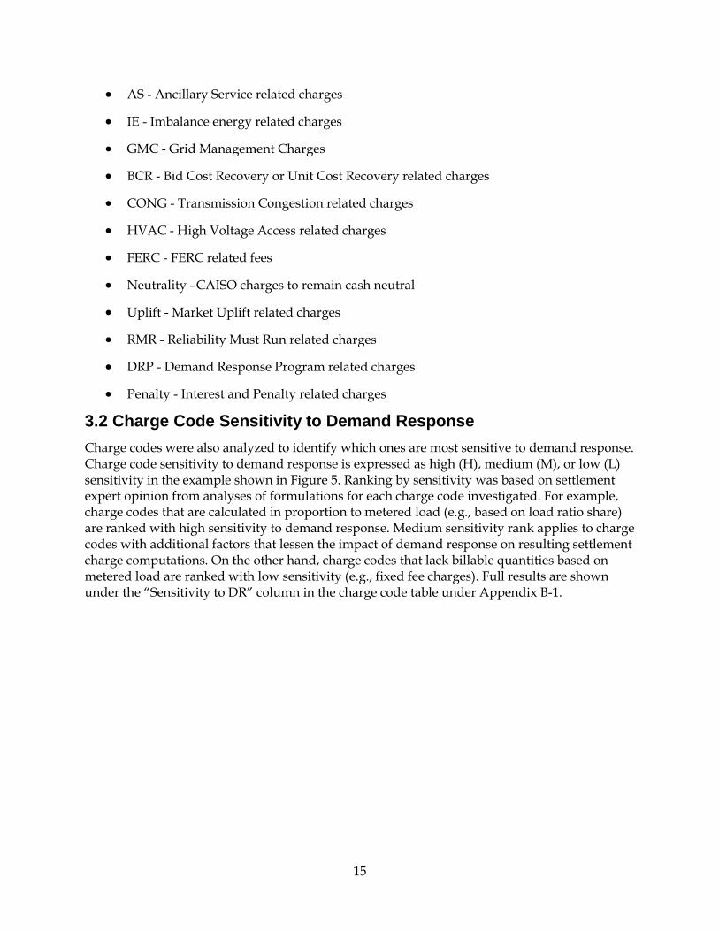
3.2 Charge Code Sensitivity to Demand Response Charge codes were also analyzed to identify which ones are most sensitive to demand response. Charge code sensitivity to demand response is expressed as high (H), medium (M), or low (L) sensitivity in the example shown in Figure 5. Ranking by sensitivity was based on settlement expert opinion from analyses of formulations for each charge code investigated. For example, charge codes that are calculated in proportion to metered load (e.g., based on load ratio share) are ranked with high sensitivity to demand response. Medium sensitivity rank applies to charge codes with additional factors that lessen the impact of demand response on resulting settlement charge computations. On the other hand, charge codes that lack billable quantities based on metered load are ranked with low sensitivity (e.g., fixed fee charges). Full results are shown under the “Sensitivity to DR” column in the charge code table under Appendix B-1.

15

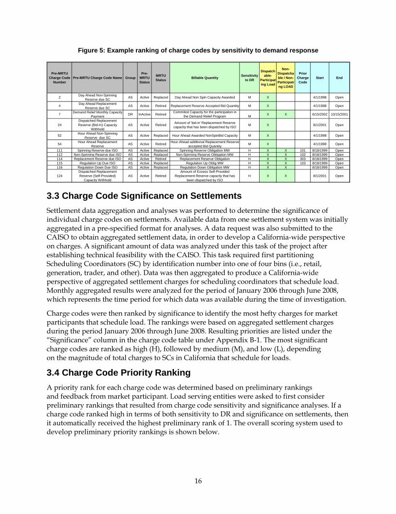
Figure 5: Example ranking of charge codes by sensitivity to demand response

Pre-MRTU Charge Code

NumberPre-MRTU Charge Code Name Group

Pre-MRTU Status

MRTU Status Billable Quantity Sensitivity

to DR

Dispatchable-

Participating Load

Non-Dispatchable / Non-Participating LOAD

Prior Charge Code

Start End

2 Day Ahead Non-Spinning Reserve due SC AS Active Replaced Day Ahead Non Spin Capacity Awarded M X 4/1/1998 Open

4 Day Ahead Replacement Reserve due SC AS Active Retired Replacement Reserve Accepted Bid Quantity M X 4/1/1998 Open

7 Demand Relief Monthly Capacity Payment DR InActive Retired Commited Capacity for the participation in

the Demand Relief Program M X X 6/15/2002 10/15/2001

24Dispatched Replacement Reserve (Bid-In) Capacity

WithholdAS Active Retired Amount of 'bid-in' Replacement Reserve

capacity that has been dispatched by ISO M X 8/1/2001 Open

52 Hour Ahead Non-Spinning Reserve due SC AS Active Replaced Hour Ahead Awarded NonSpinBid Capacity M X 4/1/1998 Open

54 Hour Ahead Replacement Reserve AS Active Retired Hour-Ahead additional Replacement Reserve

accepted Bid Quantity M X 4/1/1998 Open

111 Spinning Reserve due ISO AS Active Replaced Spinning Reserve Obligation MW H X X 101 8/18/1999 Open112 Non-Spinning Reserve due ISO AS Active Replaced Non-Spinning Reserve Obligation MW H X X 102 8/18/1999 Open114 Replacement Reserve due ISO AS Active Retired Replacement Reserve Obligation H X X 303 8/18/1999 Open115 Regulation Up Due ISO AS Active Replaced Regulation Up Oblig MW H X X 103 8/18/1999 Open116 Regulation Down Due ISO AS Active Replaced Regulation Down Obligation MW H X X 8/18/1999 Open

124Dispatched Replacement Reserve (Self-Provided)

Capacity WithholdAS Active Retired

Amount of Excess Self-Provided Replacement Reserve capacity that has

been dispatched by ISOH X X 8/1/2001 Open

3.3 Charge Code Significance on Settlements Settlement data aggregation and analyses was performed to determine the significance of individual charge codes on settlements. Available data from one settlement system was initially aggregated in a pre-specified format for analyses. A data request was also submitted to the CAISO to obtain aggregated settlement data, in order to develop a California-wide perspective on charges. A significant amount of data was analyzed under this task of the project after establishing technical feasibility with the CAISO. This task required first partitioning Scheduling Coordinators (SC) by identification number into one of four bins (i.e., retail, generation, trader, and other). Data was then aggregated to produce a California-wide perspective of aggregated settlement charges for scheduling coordinators that schedule load. Monthly aggregated results were analyzed for the period of January 2006 through June 2008, which represents the time period for which data was available during the time of investigation.

Charge codes were then ranked by significance to identify the most hefty charges for market participants that schedule load. The rankings were based on aggregated settlement charges during the period January 2006 through June 2008. Resulting priorities are listed under the “Significance” column in the charge code table under Appendix B-1. The most significant charge codes are ranked as high (H), followed by medium (M), and low (L), depending on the magnitude of total charges to SCs in California that schedule for loads.

3.4 Charge Code Priority Ranking A priority rank for each charge code was determined based on preliminary rankings and feedback from market participant. Load serving entities were asked to first consider preliminary rankings that resulted from charge code sensitivity and significance analyses. If a charge code ranked high in terms of both sensitivity to DR and significance on settlements, then it automatically received the highest preliminary rank of 1. The overall scoring system used to develop preliminary priority rankings is shown below.

16

Sensitivity Significance Priority Rank

H H 1 (highest)

M H 2

H M 3

M M 4

other other 5 (lowest)

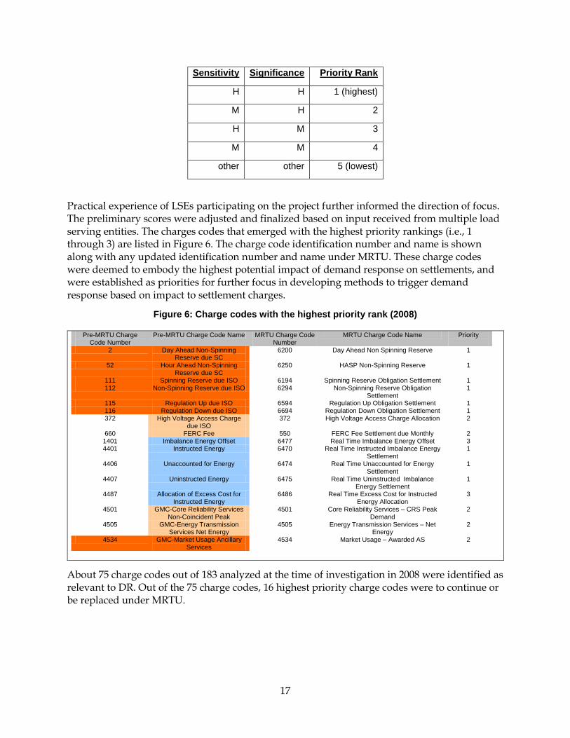
Practical experience of LSEs participating on the project further informed the direction of focus. The preliminary scores were adjusted and finalized based on input received from multiple load serving entities. The charges codes that emerged with the highest priority rankings (i.e., 1 through 3) are listed in Figure 6. The charge code identification number and name is shown along with any updated identification number and name under MRTU. These charge codes were deemed to embody the highest potential impact of demand response on settlements, and were established as priorities for further focus in developing methods to trigger demand response based on impact to settlement charges.

Figure 6: Charge codes with the highest priority rank (2008)

Pre-MRTU Charge Code Number

Pre-MRTU Charge Code Name MRTU Charge Code Number

MRTU Charge Code Name Priority

2 Day Ahead Non-Spinning Reserve due SC

6200 Day Ahead Non Spinning Reserve 1

52 Hour Ahead Non-Spinning Reserve due SC

6250 HASP Non-Spinning Reserve 1

111 Spinning Reserve due ISO 6194 Spinning Reserve Obligation Settlement 1 112 Non-Spinning Reserve due ISO 6294 Non-Spinning Reserve Obligation

Settlement 1

115 Regulation Up due ISO 6594 Regulation Up Obligation Settlement 1 116 Regulation Down due ISO 6694 Regulation Down Obligation Settlement 1 372 High Voltage Access Charge

due ISO 372 High Voltage Access Charge Allocation 2

660 FERC Fee 550 FERC Fee Settlement due Monthly 2 1401 Imbalance Energy Offset 6477 Real Time Imbalance Energy Offset 3 4401 Instructed Energy 6470 Real Time Instructed Imbalance Energy

Settlement 1

4406 Unaccounted for Energy 6474 Real Time Unaccounted for Energy Settlement

1

4407 Uninstructed Energy 6475 Real Time Uninstructed Imbalance Energy Settlement

1

4487 Allocation of Excess Cost for Instructed Energy

6486 Real Time Excess Cost for Instructed Energy Allocation

3

4501 GMC-Core Reliability Services Non-Coincident Peak

4501 Core Reliability Services – CRS Peak Demand

2

4505 GMC-Energy Transmission Services Net Energy

4505 Energy Transmission Services – Net Energy

2

4534 GMC-Market Usage Ancillary Services

4534 Market Usage – Awarded AS 2

About 75 charge codes out of 183 analyzed at the time of investigation in 2008 were identified as relevant to DR. Out of the 75 charge codes, 16 highest priority charge codes were to continue or be replaced under MRTU.

17

CHAPTER 4: Demand Response Trigger Methodology Development

4.1 Foundation This section describes the theoretical foundation for a method developed under the project to trigger demand response in a way that connects retail load to latest wholesale cost conditions. Based on the priorities identified earlier, the project team developed a methodology for determining the impact of demand response on highest priority charges. The methodology applies a basic definition of demand response. Namely, “demand response is a dynamic change in electricity usage coordinated with power system or market conditions” [3]. Therefore, the impact of demand response on any particular settlement charge is the derivative of the charge with respect to demand (or metered load).

To determine the impact of demand response on overall market settlements for any particular SC that schedules load, one would compute the derivative of the sum of settlement charges allocable to the SC with respect to the SC’s metered load. Since the derivative of a sum is equal to the sum of the derivatives (as in Equation 1), it follows that the impact of demand response on an SC’s settlements can be computed as the sum of demand response impacts on each charge code allocable to the SC.

Utilizing a top-down approach to direct further project focus, the project team proceeded according to the priorities identified in the previous project task. That is, the team derived analytical formulations for computing the derivatives of highest priority charge codes that received a ranking of 1. As indicated in Figure 6, these highest priority charge codes include Ancillary Service related charge codes (e.g., Charge Code 2, 52, 111, 112, 115, 116, and 4534) and Imbalance Energy charge codes (e.g., Charge Code 4401, 4406, and 4407). The remainder of this section summarizes the resulting derived formulations.

The basic principle from Calculus shown in Equation 1 is applied in subsequent derivations. In words, the equation states that the derivative of a sum of charges, denoted by Ci and expressed as a function of metered load L, is equal to sum of the derivatives with respect to metered load L.

Equation 1: The derivative of a sum of is the sum of the derivatives

)(

)(

∑∑

∂∂

=∂

∂

i

iii

LLC

L

LC

4.2 Analytical Derivations Analytical derivations for ancillary service charge codes are given next. The formulas identified below can be used to compute “a change in charge due to a change in metered load” for the charge codes specified. These formulas were derived through careful analyses and domain expert knowledge of the operations and settlements process of the California electricity

18

markets. The derivations were distributed to personnel on the wholesale side of participant organizations for a second opinion as well. Results are summarized below.

The impact of demand response on Ancillary Service charges, as a collective category of charges, can be computed as follows.

That is, the impact of demand response on each Ancillary Service charge is first computed taking derivatives. The results are then summed. The resulting analytical formulations for approximating the derivative of each Ancillary Service charge code are shown below for Charge Codes 111, 112, 115, 116, and 4534. Assumptions that were made to simplify the derivative computations are also listed. Detailed step-by-step derivations are provided in the Appendix of this report.

The formulations below were derived before the California market transitioned under Market Redesign and Technology Upgrade (MRTU) in April 2009. They are provided here as examples of applying the DR trigger methodology to determine the impact of triggering demand response based on Ancillary Service charges. Additional formulations have been subsequently derived for charge codes that have come into effect under MRTU, in order to support proof-of-concept development stages of the project.

s"derivative theof sum theis sum a of derivative The" )()(

Since ∑∑

∂∂

=∂

∂

i

iii

LLC

L

LC

.

Then

LoadCharge

LoadCharge

LoadCharge

LoadCharge

LoadCharge

LoadCharge eASGMCMktUsagRegDownRegUpNSpinSpinASGroup

∆

∆+

∆

∆+

∆

∆+

∆

∆+

∆

∆=

∆

∆

.Let eASGMCMktUsagRegDownRegUpNSpinSpinASGroup ChargeChargeChargeChargeChargeCharge ++++=

19

Equation 2: Derivation for Charge Code 111 (“Spinning Reserve due ISO”)

Assumption made in the derivation above include:

1. The following variables assumed to be independent of demand response: SpinRate, InterSCSpinSold, InterSCSpinBought, EffectiveSelfProvidedSpin, SpinReqHA, SpinReqDA, TotalEffSelfProvSpin

2. The change in SC’s BaseOpReserveReq due to a change in its Load is negligible compared to the sum of the BaseOpReserveReq of all other SCs.

Equation 3: Derivation for Charge Code 112 (“Non Spinning Reserve due ISO”)

Assumption made in the derivation above include:

( )Load

rveReqBaseOpReseqpReserveReTotalBaseO

lfProvSpinTotalEffSeSpinReqHASpinReqDASpinRateLoad

Charge∆

∆∗

++≈

∆∆ *111

( ) 07.0* ∗

++≈

∆∆

qpReserveReTotalBaseOlfProvSpinTotalEffSeSpinReqHASpinReqDASpinRate

LoadCharge

.Let ImportExportdMeteredLoaNetload −+=

then, If HydroNetload >=

( ) 05.0* ∗

++≈

∆∆

qpReserveReTotalBaseOlfProvSpinTotalEffSeSpinReqHASpinReqDASpinRate

LoadCharge

then, If HydroNetload <

( )Load

rveReqBaseOpReseqpReserveReTotalBaseO

nlfProvNSpiTotalEffSeNSpinReqHANSpinReqDANSpinRateLoad

Charge∆

∆∗

++≈

∆∆ *112

( ) 07.0 *∗

++≈

∆∆

qpReserveReTotalBaseOnlfProvNSpiTotalEffSeNSpinReqHANSpinReqDANSpinRate

LoadCharge

.Let ImportExportdMeteredLoaNetload −+=

then, If HydroNetload >=

( ) 05.0* ∗

++≈

∆∆

qpReserveReTotalBaseOnlfProvNSpiTotalEffSeNSpinReqHANSpinReqDANSpinRate

LoadCharge

then, If HydroNetload <

20

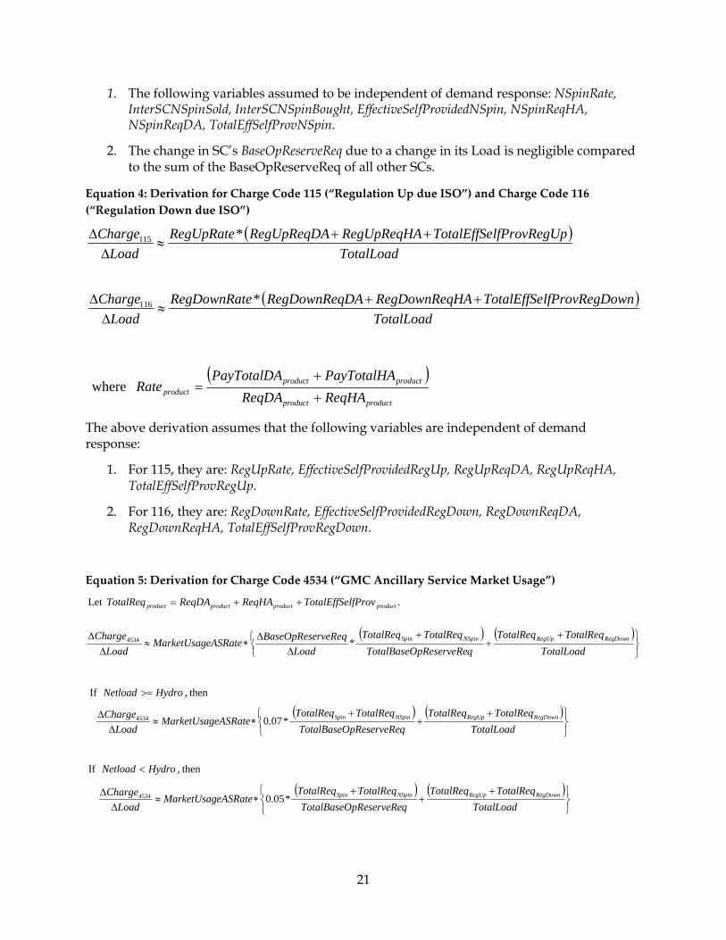
1. The following variables assumed to be independent of demand response: NSpinRate, InterSCNSpinSold, InterSCNSpinBought, EffectiveSelfProvidedNSpin, NSpinReqHA, NSpinReqDA, TotalEffSelfProvNSpin.

2. The change in SC’s BaseOpReserveReq due to a change in its Load is negligible compared to the sum of the BaseOpReserveReq of all other SCs.

Equation 4: Derivation for Charge Code 115 (“Regulation Up due ISO”) and Charge Code 116 (“Regulation Down due ISO”)

The above derivation assumes that the following variables are independent of demand response:

1. For 115, they are: RegUpRate, EffectiveSelfProvidedRegUp, RegUpReqDA, RegUpReqHA, TotalEffSelfProvRegUp.

2. For 116, they are: RegDownRate, EffectiveSelfProvidedRegDown, RegDownReqDA, RegDownReqHA, TotalEffSelfProvRegDown.

Equation 5: Derivation for Charge Code 4534 (“GMC Ancillary Service Market Usage”)

( )TotalLoad

plfProvRegUTotalEffSeRegUpReqHARegUpReqDARegUpRateLoad

Charge ++≈

∆∆ *115

( )TotalLoad

ownlfProvRegDTotalEffSeHARegDownReqDARegDownReqeRegDownRatLoad

Charge ++≈

∆∆ *116

( )productproduct

productproductproduct ReqHAReqDA

PayTotalHAPayTotalDARate

+

+= where

then, If HydroNetload >=

then, If HydroNetload <

( ) ( )+

++

∆∆

∗≈∆

∆TotalLoad

TotalReqTotalReqqpReserveReTotalBaseO

TotalReqTotalReqLoad

rveReqBaseOpReseeASRateMarketUsagLoad

Charge RegDownRegUpNSpinSpin *4534

.Let productproductproductproduct lfProvTotalEffSeReqHAReqDATotalReq ++=

( ) ( )

+

++

∗≈∆

∆TotalLoad

TotalReqTotalReqqpReserveReTotalBaseO

TotalReqTotalReqeASRateMarketUsag

LoadCharge RegDownRegUpNSpinSpin

*07.04534

( ) ( )

+

++

∗≈∆

∆TotalLoad

TotalReqTotalReqqpReserveReTotalBaseO

TotalReqTotalReqeASRateMarketUsag

LoadCharge RegDownRegUpNSpinSpin

*05.04534

21

Assumptions used in the derivation above include:

1. The same assumptions used in the derivations for Charge Codes 111,112,115,116.

2. Billable Quantities for Spin, NonSpin, RegUp, RegDown are all non-negative.

Equation 6: Derivation for Charge Code 4407 (“Uninstructed Energy”)

For this derivation, the variables assumed to be independent of demand response included: Hour-Ahead Schedules (S), Instructed Imbalance Energy (IIE), Instructed Imbalance Regulation Energy, Total Instructed Imbalance Energy, 5-min Zonal Price, Resource Specific Price, and Zonal Ex-Post Price.

4.3 Summary of Demand Response Trigger Method The charge codes of interest are the ones most sensitive to demand response and most significant on settlements. Having reviewed results of the settlement and data analyses conducted, market participants informing the project identified Imbalance Energy charges and Ancillary Service charges as the highest priority categories of charges for further investigation under Phase 1 of the project. This section summarizes the methodology developed for triggering based on imbalance energy charges (e.g., Charge Code 4407) and Ancillary Service charges (i.e., Charge Codes 111, 112, 115, 116, 4534).

Although Charge Codes 4401, 2, and 52 also fall under the highest priority categories, the project team decided to not include them in developing a trigger method, given that these charge codes are used to account for revenue sources to market participants. Since these charge codes account for revenues “due SC”, they rely on other factors like bidding strategy of market participants, which was decided not the focus under Phase 1. Rather, the team focused on actual charges that can be avoided through demand response coordinated with system or market conditions.

After determining the highest priority charge codes to develop a trigger methodology for, the project team then considered availability of information sources required as inputs to the derivative calculations. Input data available in operational timeframes was also assessed and identified in order to support operational decision-making. The resulting demand response trigger methodology is summarized in algorithm form below, using the highest priority charge code categories as examples.

Triggering based on Ancillary Service Charges

1. Understand settlement charge formula for each priority Ancillary Service charge code

4407ex post

Charge PLoad −

∆= −

∆

22

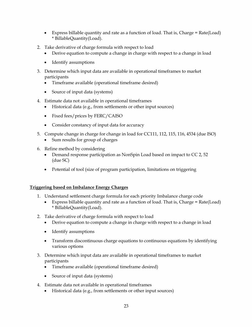
• Express billable quantity and rate as a function of load. That is, Charge = Rate(Load) * BillableQuantity(Load).

2. Take derivative of charge formula with respect to load • Derive equation to compute a change in charge with respect to a change in load

• Identify assumptions

3. Determine which input data are available in operational timeframes to market participants • Timeframe available (operational timeframe desired)

• Source of input data (systems)

4. Estimate data not available in operational timeframes • Historical data (e.g., from settlements or other input sources)

• Fixed fees/prices by FERC/CAISO

• Consider constancy of input data for accuracy

5. Compute change in charge for change in load for CC111, 112, 115, 116, 4534 (due ISO) • Sum results for group of charges

6. Refine method by considering • Demand response participation as NonSpin Load based on impact to CC 2, 52

(due SC)

• Potential of tool (size of program participation, limitations on triggering

Triggering based on Imbalance Energy Charges

1. Understand settlement charge formula for each priority Imbalance charge code • Express billable quantity and rate as a function of load. That is, Charge = Rate(Load)

* BillableQuantity(Load).

2. Take derivative of charge formula with respect to load • Derive equation to compute a change in charge with respect to a change in load

• Identify assumptions

• Transform discontinuous charge equations to continuous equations by identifying various options

3. Determine which input data are available in operational timeframes to market participants • Timeframe available (operational timeframe desired)

• Source of input data (systems)

4. Estimate data not available in operational timeframes • Historical data (e.g., from settlements or other input sources)

23

• Fixed fees/prices by FERC/CAISO

• Consider constancy of input data for accuracy

5. Compute change in charge for change in load for CC4407, 6475 (under MRTU) • Sum results for group of charges

6. Refine method by considering • Demand response participation based on impact to CC 4401 (due SC)

• Potential of tool (size of program participation, limitations on triggering

24

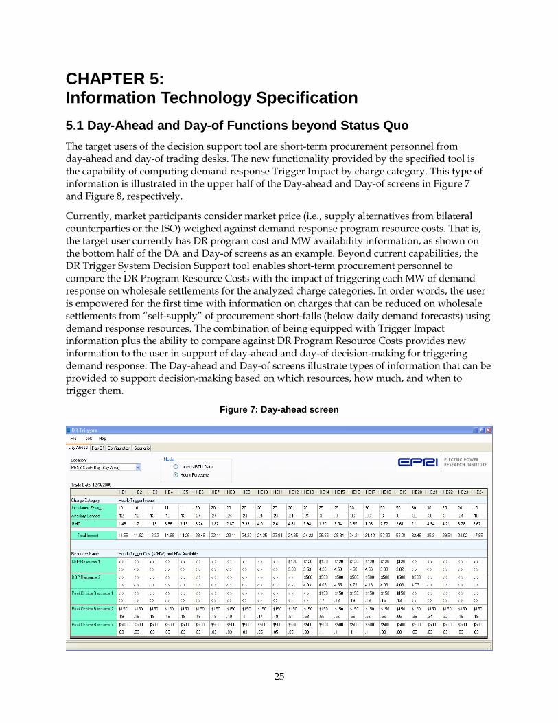
CHAPTER 5: Information Technology Specification 5.1 Day-Ahead and Day-of Functions beyond Status Quo The target users of the decision support tool are short-term procurement personnel from day-ahead and day-of trading desks. The new functionality provided by the specified tool is the capability of computing demand response Trigger Impact by charge category. This type of information is illustrated in the upper half of the Day-ahead and Day-of screens in Figure 7 and Figure 8, respectively.

Currently, market participants consider market price (i.e., supply alternatives from bilateral counterparties or the ISO) weighed against demand response program resource costs. That is, the target user currently has DR program cost and MW availability information, as shown on the bottom half of the DA and Day-of screens as an example. Beyond current capabilities, the DR Trigger System Decision Support tool enables short-term procurement personnel to compare the DR Program Resource Costs with the impact of triggering each MW of demand response on wholesale settlements for the analyzed charge categories. In order words, the user is empowered for the first time with information on charges that can be reduced on wholesale settlements from “self-supply” of procurement short-falls (below daily demand forecasts) using demand response resources. The combination of being equipped with Trigger Impact information plus the ability to compare against DR Program Resource Costs provides new information to the user in support of day-ahead and day-of decision-making for triggering demand response. The Day-ahead and Day-of screens illustrate types of information that can be provided to support decision-making based on which resources, how much, and when to trigger them.

Figure 7: Day-ahead screen

25

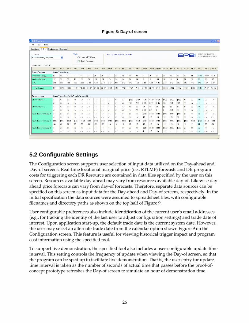
Figure 8: Day-of screen

5.2 Configurable Settings The Configuration screen supports user selection of input data utilized on the Day-ahead and Day-of screens. Real-time locational marginal price (i.e., RTLMP) forecasts and DR program costs for triggering each DR Resource are contained in data files specified by the user on this screen. Resources available day-ahead may vary from resources available day-of. Likewise day-ahead price forecasts can vary from day-of forecasts. Therefore, separate data sources can be specified on this screen as input data for the Day-ahead and Day-of screens, respectively. In the initial specification the data sources were assumed to spreadsheet files, with configurable filenames and directory paths as shown on the top half of Figure 9.

User configurable preferences also include identification of the current user’s email addresses (e.g., for tracking the identity of the last user to adjust configuration settings) and trade date of interest. Upon application start-up, the default trade date is the current system date. However, the user may select an alternate trade date from the calendar option shown Figure 9 on the Configuration screen. This feature is useful for viewing historical trigger impact and program cost information using the specified tool.

To support live demonstration, the specified tool also includes a user-configurable update time interval. This setting controls the frequency of update when viewing the Day-of screen, so that the program can be sped up to facilitate live demonstration. That is, the user entry for update time interval is taken as the number of seconds of actual time that passes before the proof-of-concept prototype refreshes the Day-of screen to simulate an hour of demonstration time.

26

Figure 9: Configuration screen

5.3 What-if Analyses The What-if screen supports decision-making through user definition and comparison of distinct scenarios. What-if calculations consider DR program incentive costs versus market price for resources procured through bilateral or ISO market alternatives, given the trigger impact for user-selected DA or Day-of timeframes.

The location option in the upper right hand corner of the screen allows selection of the location of resources that will show on the screen. This option determines the location for the Hourly Trigger Impact calculations as well.

As illustrated on the lower half of Figure 10, the What-if screen allows the user to define multiple scenarios. The user selects the name of resources to consider under each scenario and the MW quantity of each resource. The user clicks on the option “Calculate” to compute and show Net results for each user-defined resource scenario. The difference between Net results of the two defined scenarios is computed and shown on the last row on the screen, for comparison purposes. The Net calculation includes the hour-ending intervals with radio buttons clicked for the resources that are checked by the user. The tool can compute the Net for each hour-ending interval as:

Net = SumoverselectedDRResources{(TotalImpact+DRProgramCost)*MW_DRResource}

+ SumoverselectedMarketResources{(MarketPrice*MW_MktResource)}

27

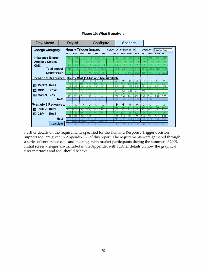
Figure 10: What-if analysis

Further details on the requirements specified for the Demand Response Trigger decision support tool are given in Appendix B-3 of this report. The requirements were gathered through a series of conference calls and meetings with market participants during the summer of 2009. Initial screen designs are included in the Appendix with further details on how the graphical user interfaces and tool should behave.

28

CHAPTER 6: Potential Benefits The trigger method developed was applied against historical data to assess potential benefits of triggering based on impact to Ancillary Service and Imbalance Energy charges. Potential benefits were assessed using historical data based on the trigger impact equations derived in Section 4.

6.1 Potential Impact on Ancillary Service Charges The investigation commenced with analysis of the impact of triggering demand response based on Ancillary Service charges during the top intervals of the period of interest. The period analyzed was from January 1, 2008 through November 30, 2008. Top intervals during this period are the hourly intervals for which demand response is determined to have the greatest charge savings.

Figure 11 lists values (in red) for the trigger impact resulting from the derivative calculations using historical data. The figure also lists the factors and components (shown in black numbers) that comprise the trigger impact calculations. Each row shows components and resulting calculations for a one-hour interval on a specified date during the period of analyses.

29

Figure 11: Hourly potential benefit calculations for triggering based on ancillary service charges (1/1/08-11/30/08)

Results are summarized below and represent the potential benefit of triggering 1 MW of demand response during the highest impact hourly intervals across the eleven month period of analyses.

Intervals Triggered Avoided Ancillary Service Charge ($/MW)

317 intervals, each with Trigger Value>$2.5/MW 2155.28

53 intervals, each with Trigger Value >$10/MW 836

37 intervals, each with Trigger Value >$12.5/MW 652.76

24 intervals, each with Trigger Value > $14.75/MW 472.22

All intervals during 11 months (8015 hourly intervals) 7266.81

30

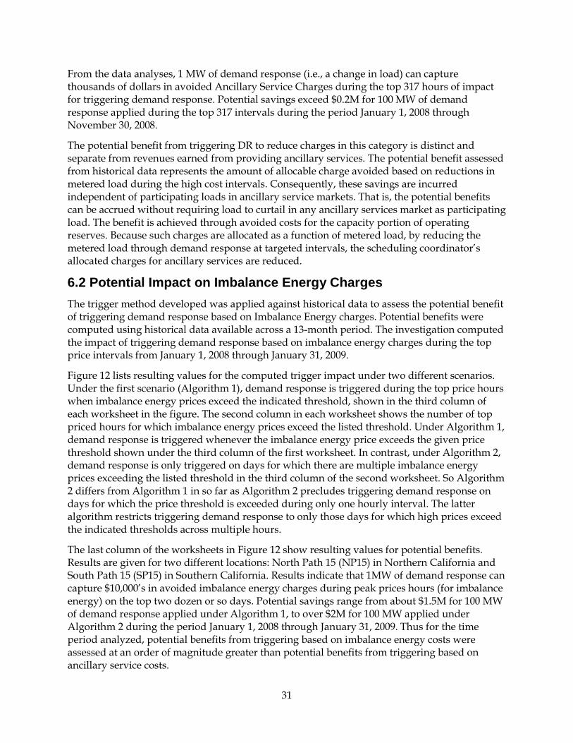
From the data analyses, 1 MW of demand response (i.e., a change in load) can capture thousands of dollars in avoided Ancillary Service Charges during the top 317 hours of impact for triggering demand response. Potential savings exceed $0.2M for 100 MW of demand response applied during the top 317 intervals during the period January 1, 2008 through November 30, 2008.

The potential benefit from triggering DR to reduce charges in this category is distinct and separate from revenues earned from providing ancillary services. The potential benefit assessed from historical data represents the amount of allocable charge avoided based on reductions in metered load during the high cost intervals. Consequently, these savings are incurred independent of participating loads in ancillary service markets. That is, the potential benefits can be accrued without requiring load to curtail in any ancillary services market as participating load. The benefit is achieved through avoided costs for the capacity portion of operating reserves. Because such charges are allocated as a function of metered load, by reducing the metered load through demand response at targeted intervals, the scheduling coordinator’s allocated charges for ancillary services are reduced.

6.2 Potential Impact on Imbalance Energy Charges The trigger method developed was applied against historical data to assess the potential benefit of triggering demand response based on Imbalance Energy charges. Potential benefits were computed using historical data available across a 13-month period. The investigation computed the impact of triggering demand response based on imbalance energy charges during the top price intervals from January 1, 2008 through January 31, 2009.

Figure 12 lists resulting values for the computed trigger impact under two different scenarios. Under the first scenario (Algorithm 1), demand response is triggered during the top price hours when imbalance energy prices exceed the indicated threshold, shown in the third column of each worksheet in the figure. The second column in each worksheet shows the number of top priced hours for which imbalance energy prices exceed the listed threshold. Under Algorithm 1, demand response is triggered whenever the imbalance energy price exceeds the given price threshold shown under the third column of the first worksheet. In contrast, under Algorithm 2, demand response is only triggered on days for which there are multiple imbalance energy prices exceeding the listed threshold in the third column of the second worksheet. So Algorithm 2 differs from Algorithm 1 in so far as Algorithm 2 precludes triggering demand response on days for which the price threshold is exceeded during only one hourly interval. The latter algorithm restricts triggering demand response to only those days for which high prices exceed the indicated thresholds across multiple hours.

The last column of the worksheets in Figure 12 show resulting values for potential benefits. Results are given for two different locations: North Path 15 (NP15) in Northern California and South Path 15 (SP15) in Southern California. Results indicate that 1MW of demand response can capture $10,000’s in avoided imbalance energy charges during peak prices hours (for imbalance energy) on the top two dozen or so days. Potential savings range from about $1.5M for 100 MW of demand response applied under Algorithm 1, to over $2M for 100 MW applied under Algorithm 2 during the period January 1, 2008 through January 31, 2009. Thus for the time period analyzed, potential benefits from triggering based on imbalance energy costs were assessed at an order of magnitude greater than potential benefits from triggering based on ancillary service costs.

31

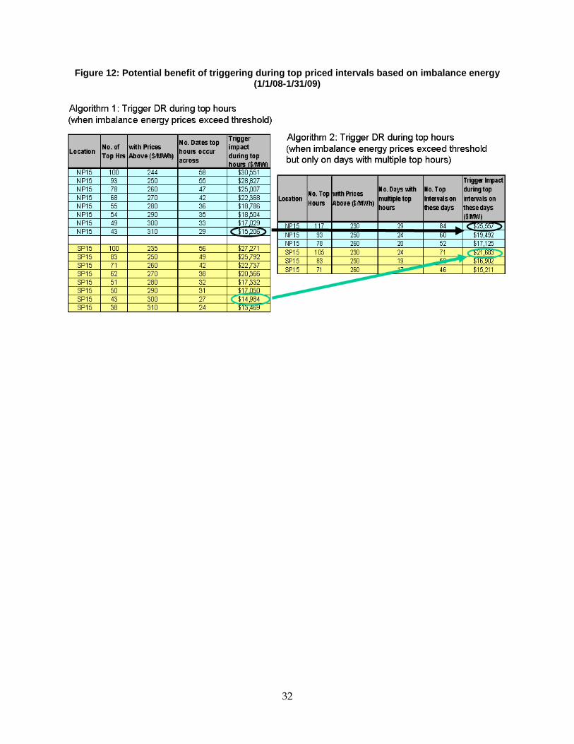
Figure 12: Potential benefit of triggering during top priced intervals based on imbalance energy (1/1/08-1/31/09)

32

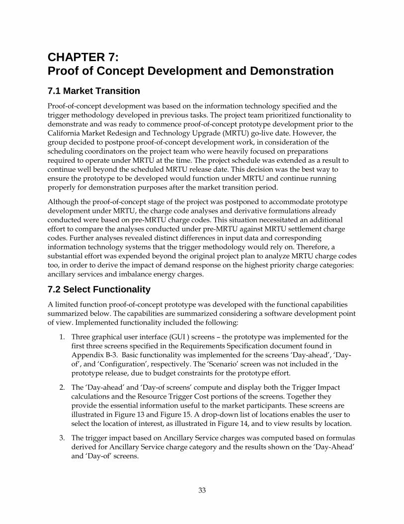
CHAPTER 7: Proof of Concept Development and Demonstration 7.1 Market Transition Proof-of-concept development was based on the information technology specified and the trigger methodology developed in previous tasks. The project team prioritized functionality to demonstrate and was ready to commence proof-of-concept prototype development prior to the California Market Redesign and Technology Upgrade (MRTU) go-live date. However, the group decided to postpone proof-of-concept development work, in consideration of the scheduling coordinators on the project team who were heavily focused on preparations required to operate under MRTU at the time. The project schedule was extended as a result to continue well beyond the scheduled MRTU release date. This decision was the best way to ensure the prototype to be developed would function under MRTU and continue running properly for demonstration purposes after the market transition period.

Although the proof-of-concept stage of the project was postponed to accommodate prototype development under MRTU, the charge code analyses and derivative formulations already conducted were based on pre-MRTU charge codes. This situation necessitated an additional effort to compare the analyses conducted under pre-MRTU against MRTU settlement charge codes. Further analyses revealed distinct differences in input data and corresponding information technology systems that the trigger methodology would rely on. Therefore, a substantial effort was expended beyond the original project plan to analyze MRTU charge codes too, in order to derive the impact of demand response on the highest priority charge categories: ancillary services and imbalance energy charges.

7.2 Select Functionality A limited function proof-of-concept prototype was developed with the functional capabilities summarized below. The capabilities are summarized considering a software development point of view. Implemented functionality included the following:

1. Three graphical user interface (GUI ) screens – the prototype was implemented for the first three screens specified in the Requirements Specification document found in Appendix B-3. Basic functionality was implemented for the screens ‘Day-ahead’, ‘Day-of’, and ‘Configuration’, respectively. The ‘Scenario’ screen was not included in the prototype release, due to budget constraints for the prototype effort.

2. The ‘Day-ahead’ and ‘Day-of screens’ compute and display both the Trigger Impact calculations and the Resource Trigger Cost portions of the screens. Together they provide the essential information useful to the market participants. These screens are illustrated in Figure 13 and Figure 15. A drop-down list of locations enables the user to select the location of interest, as illustrated in Figure 14, and to view results by location.

3. The trigger impact based on Ancillary Service charges was computed based on formulas derived for Ancillary Service charge category and the results shown on the ‘Day-Ahead’ and ‘Day-of’ screens.

33

4. Rendering of trigger impact based on ‘Imbalance Energy’ depends on user’s selection of ‘Mode’.

a) If the user selects ‘Latest MRTU Data’ on either the ‘Day-ahead’ or ‘Day-of’ screens, then the application will download latest RT LMP data from CAISO MRTU public market information for display (as detailed under the ‘Day-ahead’ and ‘Day-of’ screen specifications in the Appendix B-3).

b) Alternatively, if the user selects ‘Hourly Forecasts’, then the application will read forecast data from a local spread-sheet and display the corresponding data matching the user-selected trade date and location. The forecast file used in the ‘Day-of’ screen represents day-of RT LMP forecasts and therefore is different from the Day-ahead RT LMP forecast file used in the ‘Day-ahead’ screen. Note: Both files and their locations are user-specified via the ‘Configuration’ screen shown in Figure 16.

5. The rendering of grid management charges (GMC) for both ‘Day-ahead’ and ‘Day-of’ in the proof-of-concept prototype used mocked-up data instead of live data feeds. The mocked up data for GMC is a small value compared to Imbalance Energy and Ancillary Service values shown on the screens under Trigger Impact. The mocked up data was taken as relatively constant between time intervals, to reflect the relatively constant nature of various grid management charges.

6. The rendering of ‘Total Impact’ was taken as the sum of trigger impact values for ‘Imbalance Energy’, ‘Ancillary Service’ and ‘GMC’, respectively, displayed under the same time interval.

7. Rendering of data under ‘Resource Name’ in both ‘Day-Ahead’ and ‘Day-Of’ was based on the Demand Response Program Cost files for ‘Day-Ahead’ and ‘Day-Of’ program resource costs and MW availability, respectively. Further details on rendering of the Resource Cost section of the screen in given under the “Day Ahead” and “Day-of” screen subsections in Appendix B-3.

8. The ‘Configuration’ screen allows the user to select the trade date associated with the ‘Day-ahead’ and ‘Day-of’ screens. The user may select a historic trade date or return to the current day via a calendar date selection option. User selection of trade date is illustrated in Figure 16.

34

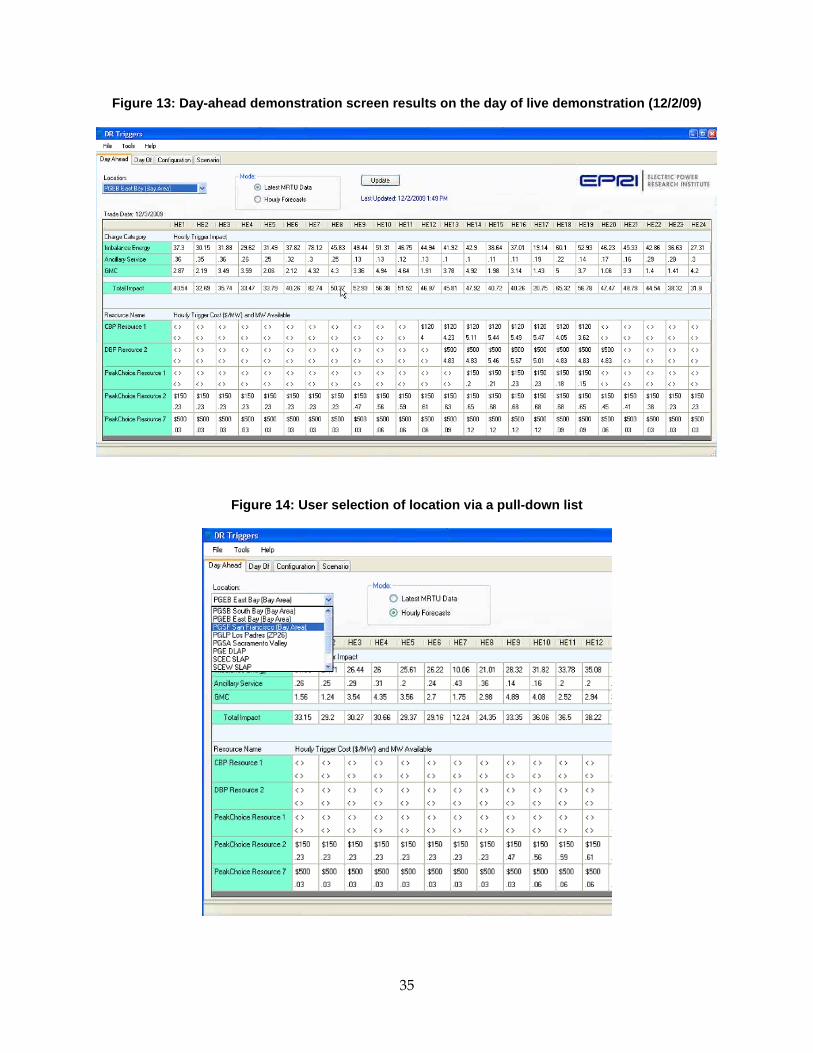
Figure 13: Day-ahead demonstration screen results on the day of live demonstration (12/2/09)

Figure 14: User selection of location via a pull-down list

35

Figure 15: Day-of demonstration screen results on day of live demonstration (12/2/09)

Figure 16: User selection of a historic trade date via a calendar date selection option

36

7.3 Live Demonstration The proof-of-concept system was implemented with select functionality to support live demonstration. The decision support tool was explained in the context of the day-in-the-life-of short term procurement personnel, beginning at the day-ahead desk, followed by the day-of desk. The demonstration highlighted information provided by the prototyped tool to support decision-making beyond the status quo of information available to the user. In particular, the tool provides the user with trigger impact information alongside program cost information, so that the user can readily discern time intervals when triggering demand response was estimated to “be in the money”.

The live demonstration illustrated how the prototyped tool supports decision-making on when (what interval of the day), which resources, where (what location), and how much demand response to trigger, based on impact to settlement charges. The live demonstration illustrated that it is feasible to estimate demand response impact on settlements in day-ahead and day-of timeframes using latest market data. Not only were the derivative calculations performed automatically during live demonstration using automated data feeds, but also the prototype was robust enough to handle cases of missing data or occasional hang-ups with the MRTU server during data downloads.

Several interesting scenarios were illustrated using the prototyped proof-of-concept system. These scenarios included:

1. Scenario A to illustrate when locations mattered: Trigger impact calculations varied substantially for select locations, so that it made sense to trigger DR resources in multiple locations but not other locations.

2. Scenario B to illustrate when trade dates mattered: On certain trade dates the tool indicated select hours that triggering demand response was estimated to be in the money. But for many other trade dates this was not the case.

3. Scenario C to illustrate when charge code matters: On certain days the trigger impact calculations for ancillary services was on a greater order of magnitude than on average

Each of these scenarios is illustrated in the following figures.

Live Demonstration of Scenario A

Figure 17 through Figure 20 provide screenshots of the live demonstration highlighting differences in triggering decisions by location for trade date November 26, 2009. Upon close examination of results for the Sacramento (Figure 17), South Bay Area (Figure 19), and East Bay Area (Figure 19) locations, the reader will note that the trigger impact is greater than the trigger costs for at least one resource during hour ending intervals 1, 2, 3, 7, and 8, respectively. Furthermore, trigger impact calculations indicate that triggering PeakChoice Resource 7 at $500/MW is in the money only during hour ending interval 7 in the Sacramento and East Bay Area locations. In contrast, there are no time intervals for which triggering demand response is in the money for any resource listed in Figure 18 for the Los Padres location.

37

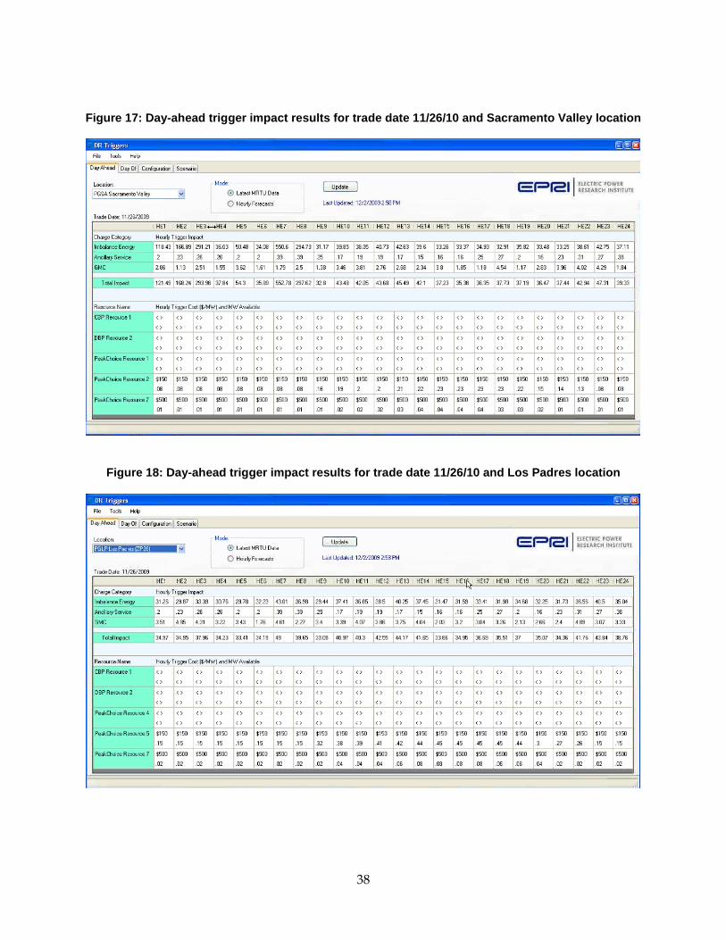
Figure 17: Day-ahead trigger impact results for trade date 11/26/10 and Sacramento Valley location

Figure 18: Day-ahead trigger impact results for trade date 11/26/10 and Los Padres location

38

Figure 19: Day-ahead trigger impact results for trade date 11/26/10 and South Bay Area location

Figure 20: Day-ahead trigger impact results for trade date 11/26/10 and East Bay Area location

39

Live Demonstration of Scenario B

The Day-ahead, Day-of, and Configuration screens were used to view results on different trades dates to illustrate Scenario C (i.e., when trade date matters). Results from the date of live demonstration (12/2/09) were shown first, followed by results for the trade date 11/25/10. Figure 13 and Figure 15 show the magnitude of trigger impact calculations on the Day-ahead and Day-of screens, respectively.

On the day of live demonstration (i.e., 12/2/09), the Day-ahead screen was demonstrated to provide estimates day-ahead for the next trade date 12/3/09, whereas the Day-of screen was demonstrated to provide trigger impact results for the current trade date 12/2/09. On both screens showing results for the day of live demonstration, there were no intervals for which triggering demand response was in the money for the default location. Different locations were selected using the drop-down list (shown in Figure 14) to conclude the same.

Results for the historic trade date 11/26/10 were also examined by selecting 11/25/10 using the calendar option under the Configuration screen (Figure 16), and then proceeding to the Day-ahead screen to view results for the next trade date 11/26/10. As explained under Scenario A, multiple hours were identified for which triggering demand response was in the money on this trade date for at least one resource in different locations.

Live Demonstration of Scenario C

Figure 21 provides a screenshot of the live demonstration of Scenario C, highlighting an instance when charge code-specific results matter. For the selected trade date 7/26/10, the Day-ahead screen was demonstrated to provide estimates of trigger impact calculations for the next trade date 7/27/10. In particular, the trigger impact values for ancillary services were an order of magnitude greater than on average during hour ending intervals 17 and 18. This example was used to highlight the situation of uncertainty surrounding system reliability and associated ancillary service charges when reliability is at stake. The California Energy Crisis of 2000-2001, which has been described as a crisis of reliability [2], was used to reinforce the notion that real-time system reliability costs can be unpredictable, and therefore must also be considered in overall demand response trigger impact calculations.

40

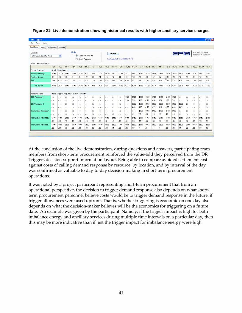
Figure 21: Live demonstration showing historical results with higher ancillary service charges

At the conclusion of the live demonstration, during questions and answers, participating team members from short-term procurement reinforced the value-add they perceived from the DR Triggers decision-support information layout. Being able to compare avoided settlement cost against costs of calling demand response by resource, by location, and by interval of the day was confirmed as valuable to day-to-day decision-making in short-term procurement operations.

It was noted by a project participant representing short-term procurement that from an operational perspective, the decision to trigger demand response also depends on what short-term procurement personnel believe costs would be to trigger demand response in the future, if trigger allowances were used upfront. That is, whether triggering is economic on one day also depends on what the decision-maker believes will be the economics for triggering on a future date. An example was given by the participant. Namely, if the trigger impact is high for both imbalance energy and ancillary services during multiple time intervals on a particular day, then this may be more indicative than if just the trigger impact for imbalance energy were high.

41

CHAPTER 8: Future Work 8.1 Expanded Scope Phase 1 of the project focused on methodology design and development of a limited function proof-of-concept system to demonstrate feasibility of the conceived trigger impact assessment method. A subsequent project phase (Phase 2) is envisioned with expanded scope, to include investigation of additional charge codes and broad implementation of the functionality specified in Phase 1 (in Appendix B-1) for the DR Trigger decision support tool.

The broader investigation proposed for Phase 2 includes development of a conceptual framework for estimating the financial impact of demand response under distinctly different methods of integration within wholesale markets. The financial impact of demand response varies depending on the integration method assumed. Possibilities include:

1. demand response integration in wholesale markets on the supply-side2, substituting for generation supply,

2. self-use within market participant portfolios (e.g., using demand response within the market participant’s own portfolio to avoid supply-side procurement); and

3. demand response integration in wholesale markets on the demand-side, as elastic demand enabling the ISO to avoid excess procurement (beyond aggregate customer demand).

The assumed method of integrating demand response influences wholesale cost and settlement outcomes. So Phase 2 investigations would be conducted considering mutually exclusive methods of integration, including newer paradigms being discussed in industry, possibly enabled through deployment of smart grid infrastructure.

Results will be reported within a broad context of integration paradigms, utilizing the conceptual framework, which will be useful for relating different methods of integrating demand response within wholesale markets.

8.2 Conceptual Framework Development: Descriptive Framework Relating Wholesale Integration Methods Connecting retail to wholesale markets involves a continuum of requirements, including cooperation of end-use customers themselves who provide demand response. 3 Recounting

2 For example, California wholesale electricity market programs accommodating load participation include Participating Load (PL), Proxy Demand Resource (PDR), and Reliability Demand Response Program (RDRP).

3 Currently retail customers receive more compensation to participate in DR than the wholesale market is valuing DR on the basis of the cost of energy. This is understandable since the retail rate is higher than wholesale procurement cost and customers want to be compensated more than their base rate to participate in DR.

42

instances that demand response program rules compelled triggering DR at times of low or no perceived value, market participants on the project team emphasize triggering flexibility is important. Though beyond the scope of the project to design markets and DR programs, a subsequent phase of the project could clarify what methods exist for integrating demand response with wholesale markets and what critical integration challenges are being addressed by the project. These could be described within a common framework that relates existing methods as well as associates integration challenges with the methods.

Phase 2 would commence with development of a conceptual framework to describe and relate distinct methods of integrating demand response in wholesale markets. Both status quo and newer methods being discussed in industry and referenced in literature will be included in the descriptive framework. The framework will be useful for presenting overall Phase 2 findings within a common context. It will also assist the reader to quickly relate research results and identify their applicability, considering the plethora of implementations and types of demand response programs and integration methods that exist.

Another important question for Phase 2 that was identified by utility project participants is how DR programs can be linked to the developed DR Triggers Decision Support tool, in order to address the full continuum of requirements involving customers that provide the DR resources. To secure customer cooperation, customers need to understand what they are providing and why (in the form of demand response). However, currently there is a wide gap in understanding with respect to wholesale market outcomes and impacts on customers. Phase 1 of the DR Triggers project provided an initial step to bridge the gap in understanding and to clarify the financial connection between retail and wholesale markets, through the impact of demand response. Further steps to bridge the gap are needed in future work. Among conceptual gaps, Phase 2 of the project develops clarity in several critical areas described below.

Needs for conceptual clarity expressed by project participants include:

1. Clarity surrounding the connection between distinct wholesale market products and electric service received by customers, from the customer perspective.

2. The added dimensions and facets available in markets, including the choice to bid participating load resources or self-use demand response within a market participant’s portfolio.

3. As markets develop as well as enabling technologies like smart grid infrastructure, could resource adequacy requirements be reduced, and how to justify?

Considering the feedback received from project participants, the following topics to clarify conceptually are proposed for a subsequent project phase:

1. How to decompose components of electric service (including reliability) into different components that a customer can appreciate

2. How to avoid wholesale charges that would otherwise be allocated, by triggering DR.

3. How developments that could be supported by project findings link to resource adequacy requirements. For example:

43

• As markets develop and different methods of integrating demand response are considered, what types of demand-side resources will meet the industry’s objectives for resource adequacy? How could resource adequacy requirements be reduced, and how to justify?

• Currently all DR resources qualify for resource adequacy (e.g., 115% qualify whereas generation resources qualify 1MW for 1MW). As wholesale integrated DR increases in participation, is there a way to quantify the amount of resource adequacy requirement that can be reduced?

8.3 Expanded Methodology: Design, Specification, Implementation, and Demonstration Market participants noted that Phase 1 of the project broadened perspectives on charge codes and demonstrated the value of tracking additional charge codes. Beyond just looking at imbalance energy prices, the project showed the significance of considering ancillary service and other categories of charges too. The project team proposes to investigate more charge codes, beyond those studied in Phase 1. By investigating types that account for revenue sources as well as charges due to the ISO, Phase 2 will investigate additional dimensions and facets in markets, include the choice to bid or self-use demand response.

This subsection describes the steps for design, specification, implementation, and demonstration of an expanded methodology for assessing the financial impact of triggering demand response. Derivative formulations need to be developed for triggering demand response based on impact to other charge codes that have been identified as priority under Phase 1. Analyses will be conducted to identify input data, availability, and methods to connect to live data feeds, in order to support full implementation. Implementation will demonstrate specified functionality for the Day-ahead, Day-of, and What-if Scenario screens, beyond the limited-function proof-of-concept prototype. Moreover, expanded functionality will be specified in order to consider counterparty trades. The expanded scope proposed supports forming an overall perspective of the value of triggering DR, considering avoided wholesale market charges and potential revenues from both market and counterparty trades.

Step 1 (Theoretical analysis of priority charge codes for charges “due ISO”): The goal is to augment the trigger methodology based on next highest priority charge codes. This begins with calculating the derivatives of the remaining priority charge codes, in order of priority 1 through 3. In particular, analyses have yet to be conducted for the following charge codes that were identified under Phase 1:

• Unaccounted for Energy (6474) is priority 1

• Grid Management Charge (4501, 4505) and HVAC (372) are priority 2

• Allocation of Excess Cost for Imbalance Energy (6486) and FERC Fee (550) is priority 3

44

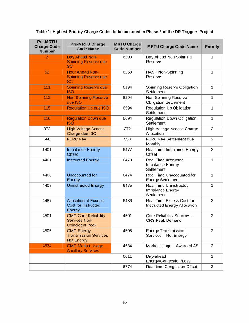
Table 1: Highest Priority Charge Codes to be included in Phase 2 of the DR Triggers Project

Pre-MRTU Charge Code

Number Pre-MRTU Charge

Code Name MRTU Charge Code Number MRTU Charge Code Name Priority

2 Day Ahead Non-Spinning Reserve due SC

6200 Day Ahead Non Spinning Reserve

1

52 Hour Ahead Non-Spinning Reserve due SC

6250 HASP Non-Spinning Reserve

1

111 Spinning Reserve due ISO

6194 Spinning Reserve Obligation Settlement

1

112 Non-Spinning Reserve due ISO

6294 Non-Spinning Reserve Obligation Settlement

1

115 Regulation Up due ISO 6594 Regulation Up Obligation Settlement

1

116 Regulation Down due ISO

6694 Regulation Down Obligation Settlement

1

372 High Voltage Access Charge due ISO

372 High Voltage Access Charge Allocation

2

660 FERC Fee 550 FERC Fee Settlement due Monthly

2

1401 Imbalance Energy Offset

6477 Real Time Imbalance Energy Offset

3

4401 Instructed Energy 6470 Real Time Instructed Imbalance Energy Settlement

1

4406 Unaccounted for Energy

6474 Real Time Unaccounted for Energy Settlement

1

4407 Uninstructed Energy 6475 Real Time Uninstructed Imbalance Energy Settlement

1

4487 Allocation of Excess Cost for Instructed Energy

6486 Real Time Excess Cost for Instructed Energy Allocation

3

4501 GMC-Core Reliability Services Non-Coincident Peak

4501 Core Reliability Services – CRS Peak Demand

2

4505 GMC-Energy Transmission Services Net Energy

4505 Energy Transmission Services – Net Energy

2

4534 GMC-Market Usage Ancillary Services

4534 Market Usage – Awarded AS 2

6011 Day-ahead Energy/Congestion/Loss

1

6774 Real-time Congestion Offset 3

45

Table 1 identifies the highest priority charge codes for inclusion in the DR Trigger method. In Phase 2, analytical derivative calculations would be performed for Priority 2 and 3 charge codes, as well as for the remaining Priority 1 charge codes: Unaccounted for Energy (UFE) and Day-ahead Energy/Congestion/Loss Settlement. The former charge code was traded out in order to include GMC Ancillary Service Market Usage charge code in the Phase 1 analyses. The latter charge code did not exist before MRTU. Nevertheless, all priority charge codes are important to analyze and consider in the overall trigger methodology.

Step 2 (Specification for automation of trigger impact calculations): The next step is to determine input data availability and specify the trigger methodology for the additional charge code derivations. Results will be displayed in place of the placeholder row labeled “GMC” in the screen below, in order to present details that expand beyond what was developed in Phase 1.

Step 3 (Trigger Methodology development considering revenue “due SC”): The next step is to expand the trigger methodology, considering installed capacity procured through counterparty trades in the bilateral market, as well as Ancillary Service supply offers by Participating Loads (i.e., Charge Codes 6200 and 6470). Considering these possible revenue sources, the task is to specify functionality and supporting information to be displayed. These must be of value to short-term procurement personnel, in order to be included for implementation.

Step 4 (Implementation and Demonstration) A subsequent step focuses on design and implementation of the Phase 2 demonstration system. Components of the system are illustrated in Figure 22 for reference. Additional features and functionality beyond the Phase 1 proof-of-concept demonstration system are also called out in the figure. In Particular, “complete timer functionalities” refers to the implementation of different cases for input data availability. Automatic updates are performed for information shown on the day-ahead and day-of screens, based on distinct cases of input data availability identified under Step 2. For example, the previous day’s data will be utilized to inform results shown on the day-ahead screen until a certain time when the next days’ day-ahead data is available or posted by the CAISO during a specified time window (e.g., 1 to 3pm).

46

Figure 22: Proposed Reference Design for Phase 2 Demonstration System

8.4 Reporting A final report will document results of conceptual framework development, analyses, and specifications. The DR Trigger Decision Support tool’s full design, implementation, and demonstration will also be documented. Potential benefits and value-add applications will also be illustrated as well as participant insights gathered through experience in testing and demonstrating the implemented system. The experiences and value perceptions of procurement personnel serving to test the tool will also be documented.

47

CHAPTER 9: Conclusion This report describes the development of a demand response trigger methodology based on impact to settlement charges. Priority was established through careful analyses of over 100 charge codes, which were narrowed down based on sensitivity to demand response and significance on settlement statements of scheduling coordinators that schedule load in California. Potential Benefits were assessed for triggering demand response using the developed methodology. Hard data was gathered to develop examples showing numerical results from applying the trigger methodology. Requirements specifications were drafted for a decision support tool that embodies the trigger methodology and performs automated trigger impact calculations based on live data streams. Findings were presented to the public via webcast at a final project workshop.

Throughout the project, numerous conference calls and a few face-to-face meetings were held with project participants. The participants included the CAISO, procurement personnel from the four largest load serving entities (LSEs) in California, and representatives from the retail organization of the major IOUs in California. The participants provided substantial in-kind effort, from aggregated data provision and requirements specification to proof-of-concept demonstration. The project benefited from the interdisciplinary expertise of the project team working in collaboration, all the way from the wholesale markets end down through market participant and the retail load serving end. The cross-cutting representation of participants on the project team was a vital ingredient towards project success in clarifying one necessary step in bridging the huge gap between retail and wholesale electricity markets.

The project addresses the financial disconnect between wholesale market conditions and retail incentives for demand response. By triggering demand response to achieve savings on wholesale electricity market charges (in both ISO and bilateral markets), retail markets can become inherently integrated with wholesale markets. Savings discovered at the wholesale level in turn provide a source of retail incentives for demand response. This is unlike traditional demand response programs that require an external source to fund demand response incentive payments.

The project demonstrates the feasibility of the developed methodology and a decision-support tool designed to reveal persistent strategies for capturing electricity cost savings, by identifying market-based financial incentives for demand response. Strategies exposed by the DR Trigger method have an inherent market connection. The method is applicable on an ongoing 24x7 basis for revealing incentives for demand response. In this way, a flexible tool has been designed and demonstrated that enables wholesale buyers of electricity to assess and avoid excess wholesale electricity charges.

The project developed charge code categorizations and a methodology for understanding the impact of demand response on wholesale market charges. The project identified charge code categories most sensitive to DR and assessed potential savings achievable through demand response. Ranking charge code categories from highest to lowest potential impact enabled concentration of efforts in areas of greatest potential impact.

48

Findings reveal groupings or categories of charges that can inform tariff design, including dynamic tariff designs. For example, the methodology could be applied in triggering a CPP event. Alternatively, numerical results from the analyses may support a rationale for unbundling retail rates to reveal reliability as a cost component distinct from energy in rate structures. Furthering conceptual clarity in such areas to support full market integration of demand response is proposed for investigation in a subsequent project phase.

The project supports improved public education on the connection between wholesale and retail markets. Concrete examples of charge reduction methods were provided towards improving understanding of market charges, which are allocated to SCs and ultimately passed down to customers that receive electric service. Project tasks address fundamental analysis needed to provide decision-makers with a better understanding of market charges and the impact of demand response on financial outcomes. Project findings assist energy retailers in assessing financial consequences of demand response and comparing resource options in sufficient time to impact settlement outcomes.

Through application of the proposed decision support tool, SCs that schedule load will gain insight to improve their strategic market positioning of demand response resources. They can also improve their readiness to accommodate market changes and regulatory mandates. In particular, early adopters can better position themselves to maximize demand response resources in meeting California’s Loading Priority Order requirements. They can gain a better understanding on how to trigger DR as a physical mechanism for hedging financial market risk, and as a form of insurance against excess market charges. In these ways, further investigation and application of the developed methodology and specified tool is expected to provide a flexible means to increase resource availability when most needed in real-time power system and market operations.

49

CHAPTER 10: References 1. Chuang, A.S., “Value of Real-time Information in Competitive Generation Markets”, Proceedings of IEEE Power Engineering Society Winter Meeting, New York, January 2002.

2. Chuang, A.S., “Assessing the Impact of Resource Availability on Electric Service Reliability Cost”, Electricity Journal, March 2004.

3. Chuang, A and Gellings, C., “Demand-side Integration for Customer Choice through Variable Service Subscription”, Proceedings of IEEE Power and Energy Society, Calgary, Canada, July 27-30, 2009.

50

CHAPTER 11: Glossary The following table lists acronyms found in the report and provides some explanations.

AB Assembly Bill. A state law passed by the legislature. CAISO California Independent System Operator. The regional transmission and market

system operator of the state of California. CEC California Energy Commission. CIEE California Institute for Energy and Environment. CPP Critical Peak Pricing. A variant of time-based electricity rates. The critical peak period

is characterized by a significantly higher price that is invoked for only a few hours or days a year during the most extreme peak demand periods.

CPUC California Public Utilities Commission. DER Distributed Energy Resources. Electric energy sources dispersed in nature that

typically include distributed generation and storage and may be interconnected with the power system at transmission or distribution level voltages.

DG Distributed Generation. Active energy sources dispersed in nature, such as a microturbine, diesel backup generator, or other standby generation that may be interconnected with the power system at transmission or distribution level voltages.

DR Demand Response. A dynamic change in electric load regarded as a valuable service to a system operator, such as customer response to prices, notifications, controls, or other signals designed to coordinate changes in electric power demand.

DSR Demand Side Resource. DRETD Demand Response Enabling Technology Development. EPRI Electric Power Research Institute. ESP Energy Service Provider. GHG Green House Gas. A gas when in high concentrations in the atmosphere contributes

to the greenhouse effect and global warming. IEPR Integrated Energy Policy Report. A 2007 report that provides an integrated

assessment of the major energy trends and issues facing the California’s electricity, natural gas, and transportation fuel sectors, and provides guidance on state energy policy.

ISO Independent System Operator. A regional system operator responsible for the reliable operation of the bulk electric transmission system in its FERC-approved geographic territory.

IT Information Technology. kW Kilowatt. A unit of measurement of power equal to 1000 watts. LSE Load Serving Entity. MD02 Market Design 2002. MRTU Market Redesign Technology Upgrade. MVA Megavolt Ampere. MW Megawatt. PG&E Pacific Gas and Electric. PIER Public Interest Energy Research. POC Proof of Concept. PV Photovoltaic. RD&D Research, Development, and Demonstration.

51

RON Research Opportunity Notice. RPS Renewable Portfolio Standard. RTO Regional Transmission Organization. A regional system operator responsible for the

reliable operation of the bulk electric transmission system in its FERC-approved geographic territory.

SC Scheduling Coordinator. a registered market participant with the independent system operator.

SCADA Supervisory Control And Data Acquisition. SCE Southern California Edison. SDG&E San Diego Gas and Electric. UDC Utility Distribution Company. UI User Interface.

52

APPENDIX A: Final Workshop Attendee List Over sixty individuals participated in-person or registered to participate by webcast for the December 2, 2009 final project workshop. In-person attendees are listed in Table 4 and webcast participants are listed in Table 2.

Table 2: Webcast Participants

Name Affiliation Daniel C. Engel Freeman, Sullivan & Co. Suresh Vadhva California State University, Sacramento Russ Tatro California State University, Sacramento Mohammad Vaziri Pacific Gas & Electric Co. Mark S. Martinez Southern California Edison Mark McGranaghan Electric Power Research Institute (EPRI) Terry Mohn BAE Systems/GridWise Alliance Ralph Martinez, PhD BAE Systems Donya He BAE Systems Matt Wakefield Electric Power Research Institute (EPRI) John R. Domingos Negawatt Finance Associates Carol Fisher Elster Group Robert (Bob) B. Frazier CenterPoint Energy Chantal Jones Commonwealth Edison Company (ComEd) David A. Chambers California Energy Commission Don Nichols American Electric Power Dr. Gordon K. Lee San Diego State University Art M. Altman Electric Power Research Institute (EPRI) H. Walter Johnson KEMA, Inc. Jim Stoupis ABB Inc. Chip Tenorio ComEd Chris Bell EnergyHub Lorraine Hwang California Institute for Energy & Environment Lily Kidd CPS Energy Adiel Guinzburg The Boeing Company Thomas M. Overman The Boeing Company David Drew Emerson Climate Technologies Matthew Forshey American Electric Power Salman Mohagheghi ABB Inc. John Hayn The Boeing Company

53

Table 3: Webcast Participants (continued)

Name Affiliation Ann Segesman Pacific Gas & Electric Co. Umesh Singh GE Energy T&D Automation Joe Lang Lincoln Electric System Belvin Louie Pacific Gas & Electric Co. Ron Hofmann California Institute for Energy & Environment Shiva Swaminathan City of Palo Alto Glenn Goldbeck Pacific Gas & Electric Co. Alva Svoboda Pacific Gas & Electric Co. Patrick Duggan Con Ed Patrick Mantey UC Santa Cruz Jeff Crowe Electric Power Research Institute (EPRI) Mary Ann Piette LBNL Dave Michel California Energy Commission

54

Table 4: In-Person attendees

Name Affiliation Bryan Neff California Energy Commission Chris Scruton California Energy Commission Consuelo Sichon California Energy Commission David Chambers California Energy Commission Jamie Patterson California Energy Commission Matt Coldwell California Energy Commission Norm Bourassa California Energy Commission Pedro Gomez California Energy Commission Steve Ghadiri California Energy Commission Charles Mee California Department of Water Resources John Goodin California ISO Muir Davis Southern California Edison Jeremy Laundergan Southern California Edison Trey Howard Southern California Edison Mark Ward Sempra Utilities Gaymond Yee CIEE Farrokh Rahimi OATI Angela Chuang Electric Power Research Institute (EPRI)

55

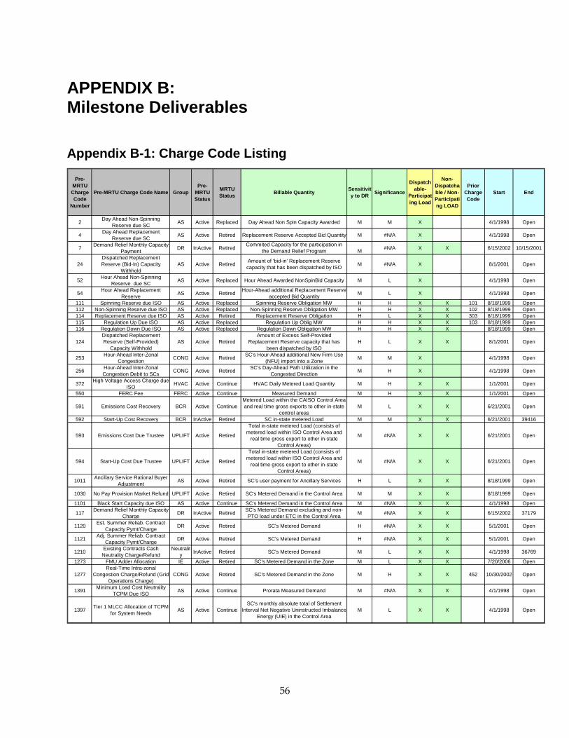
APPENDIX B: Milestone Deliverables

Appendix B-1: Charge Code Listing

Pre-MRTU Charge Code

Number

Pre-MRTU Charge Code Name GroupPre-

MRTU Status

MRTU Status Billable Quantity Sensitivit

y to DR Significance

Dispatchable-

Participating Load

Non-Dispatchable / Non-Participating LOAD

Prior Charge Code

Start End

2 Day Ahead Non-Spinning Reserve due SC AS Active Replaced Day Ahead Non Spin Capacity Awarded M M X 4/1/1998 Open

4 Day Ahead Replacement Reserve due SC AS Active Retired Replacement Reserve Accepted Bid Quantity M #N/A X 4/1/1998 Open

7 Demand Relief Monthly Capacity Payment DR InActive Retired Commited Capacity for the participation in

the Demand Relief Program M #N/A X X 6/15/2002 10/15/2001

24Dispatched Replacement Reserve (Bid-In) Capacity

WithholdAS Active Retired Amount of 'bid-in' Replacement Reserve

capacity that has been dispatched by ISO M #N/A X 8/1/2001 Open

52 Hour Ahead Non-Spinning Reserve due SC AS Active Replaced Hour Ahead Awarded NonSpinBid Capacity M L X 4/1/1998 Open

54 Hour Ahead Replacement Reserve AS Active Retired Hour-Ahead additional Replacement Reserve

accepted Bid Quantity M L X 4/1/1998 Open

111 Spinning Reserve due ISO AS Active Replaced Spinning Reserve Obligation MW H H X X 101 8/18/1999 Open112 Non-Spinning Reserve due ISO AS Active Replaced Non-Spinning Reserve Obligation MW H H X X 102 8/18/1999 Open114 Replacement Reserve due ISO AS Active Retired Replacement Reserve Obligation H L X X 303 8/18/1999 Open115 Regulation Up Due ISO AS Active Replaced Regulation Up Oblig MW H H X X 103 8/18/1999 Open116 Regulation Down Due ISO AS Active Replaced Regulation Down Obligation MW H H X X 8/18/1999 Open

124Dispatched Replacement Reserve (Self-Provided)

Capacity WithholdAS Active Retired

Amount of Excess Self-Provided Replacement Reserve capacity that has

been dispatched by ISOH L X X 8/1/2001 Open

253 Hour-Ahead Inter-Zonal Congestion CONG Active Retired SC's Hour-Ahead additional New Firm Use

(NFU) import into a Zone M M X 4/1/1998 Open

256 Hour-Ahead Inter-Zonal Congestion Debit to SCs CONG Active Retired SC's Day-Ahead Path Utilization in the

Congested Direction M H X 4/1/1998 Open

372 High Voltage Access Charge due ISO HVAC Active Continue HVAC Daily Metered Load Quantity M H X X 1/1/2001 Open

550 FERC Fee FERC Active Continue Measured Demand M H X X 1/1/2001 Open

591 Emissions Cost Recovery BCR Active ContinueMetered Load within the CAISO Control Area and real time gross exports to other in-state

control areasM L X X 6/21/2001 Open

592 Start-Up Cost Recovery BCR InActive Retired SC in-state metered Load M M X X 6/21/2001 39416

593 Emissions Cost Due Trustee UPLIFT Active Retired

Total in-state metered Load (consists of metered load within ISO Control Area and

real time gross export to other in-state Control Areas)

M #N/A X X 6/21/2001 Open

594 Start-Up Cost Due Trustee UPLIFT Active Retired

Total in-state metered Load (consists of metered load within ISO Control Area and

real time gross export to other in-state Control Areas)

M #N/A X X 6/21/2001 Open

1011 Ancillary Service Rational Buyer Adjustment AS Active Retired SC's user payment for Ancillary Services H L X X 8/18/1999 Open

1030 No Pay Provision Market Refund UPLIFT Active Retired SC's Metered Demand in the Control Area M M X X 8/18/1999 Open

1101 Black Start Capacity due ISO AS Active Continue SC's Metered Demand in the Control Area M #N/A X X 4/1/1998 Open

117 Demand Relief Monthly Capacity Charge DR InActive Retired SC's Metered Demand excluding and non-

PTO load under ETC in the Control Area M #N/A X X 6/15/2002 37179

1120 Est. Summer Reliab. Contract Capacity Pymt/Charge DR Active Retired SC's Metered Demand H #N/A X X 5/1/2001 Open

1121 Adj. Summer Reliab. Contract Capacity Pymt/Charge DR Active Retired SC's Metered Demand H #N/A X X 5/1/2001 Open

1210 Existing Contracts Cash Neutrality Charge/Refund

Neutrality InActive Retired SC's Metered Demand M L X X 4/1/1998 36769

1273 FMU Adder Allocation IE Active Retired SC's Metered Demand in the Zone M L X X 7/20/2006 Open

1277Real-Time Intra-zonal

Congestion Charge/Refund (Grid Operations Charge)

CONG Active Retired SC's Metered Demand in the Zone M H X X 452 10/30/2002 Open

1391 Minimum Load Cost Neutrality TCPM Due ISO AS Active Continue Prorata Measured Demand M #N/A X X 4/1/1998 Open

1397 Tier 1 MLCC Allocation of TCPM for System Needs AS Active Continue

SC's monthly absolute total of Settlement Interval Net Negative Uninstructed Imbalance

Energy (UIE) in the Control AreaM L X X 4/1/1998 Open

56

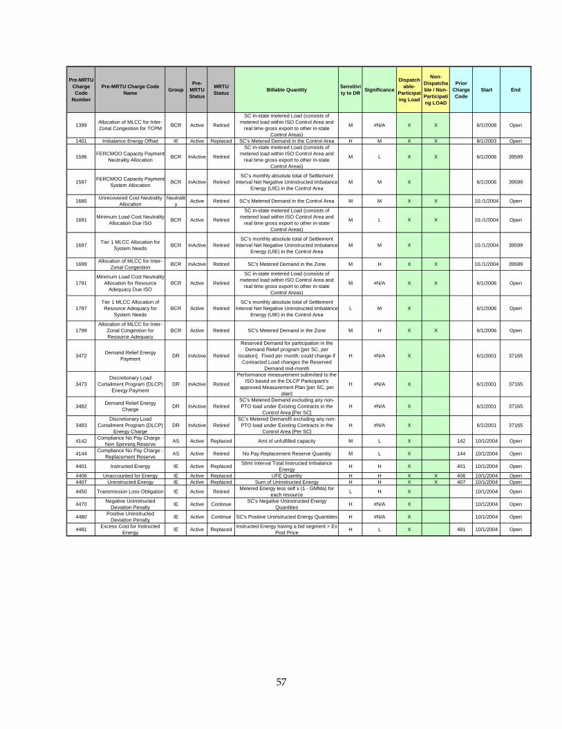
Pre-MRTU Charge Code

Number

Pre-MRTU Charge Code Name Group

Pre-MRTU Status

MRTU Status Billable Quantity Sensitivi

ty to DR Significance

Dispatchable-

Participating Load

Non-Dispatchable / Non-Participating LOAD

Prior Charge Code

Start End

1399 Allocation of MLCC for Inter-Zonal Congestion for TCPM BCR Active Retired

SC in-state metered Load (consists of metered load within ISO Control Area and

real time gross export to other in-state Control Areas)

M #N/A X X 6/1/2008 Open

1401 Imbalance Energy Offset IE Active Replaced SC's Metered Demand in the Control Area H M X X 8/1/2003 Open

1596 FERCMOO Capacity Payment Neutrality Allocation BCR InActive Retired

SC in-state metered Load (consists of metered load within ISO Control Area and

real time gross export to other in-state Control Areas)

M L X X 6/1/2006 39599

1597 FERCMOO Capacity Payment System Allocation BCR InActive Retired

SC's monthly absolute total of Settlement Interval Net Negative Uninstructed Imbalance

Energy (UIE) in the Control AreaM M X 6/1/2006 39599

1680 Unrecovered Cost Neutrality Allocation

Neutrality Active Retired SC's Metered Demand in the Control Area M M X X 10./1/2004 Open

1691 Minimum Load Cost Neutrality Allocation Due ISO BCR Active Retired

SC in-state metered Load (consists of metered load within ISO Control Area and

real time gross export to other in-state Control Areas)

M L X X 10./1/2004 Open

1697 Tier 1 MLCC Allocation for System Needs BCR InActive Retired

SC's monthly absolute total of Settlement Interval Net Negative Uninstructed Imbalance

Energy (UIE) in the Control AreaM M X 10./1/2004 39599

1699 Allocation of MLCC for Inter-Zonal Congestion BCR InActive Retired SC's Metered Demand in the Zone M H X X 10./1/2004 39599

1791Minimum Load Cost Neutrality

Allocation for Resource Adequacy Due ISO

BCR Active Retired

SC in-state metered Load (consists of metered load within ISO Control Area and

real time gross export to other in-state Control Areas)

M #N/A X X 6/1/2006 Open

1797Tier 1 MLCC Allocation of Resource Adequacy for

System NeedsBCR Active Retired

SC's monthly absolute total of Settlement Interval Net Negative Uninstructed Imbalance

Energy (UIE) in the Control AreaL M X 6/1/2006 Open

1799Allocation of MLCC for Inter-

Zonal Congestion for Resource Adequacy

BCR Active Retired SC's Metered Demand in the Zone M H X X 6/1/2006 Open

3472 Demand Relief Energy Payment DR InActive Retired

Reserved Demand for participation in the Demand Relief program [per SC, per

location]. Fixed per month; could change if Contracted Load changes the Reserved

Demand mid-month

H #N/A X 6/1/2001 37165

3473Discretionary Load

Curtailment Program (DLCP) Energy Payment

DR InActive Retired

Performance measurement submitted to the ISO based on the DLCP Participant's

approved Measurement Plan [per SC, per plan]

H #N/A X 6/1/2001 37165

3482 Demand Relief Energy Charge DR InActive Retired

SC's Metered Demand excluding any non-PTO load under Existing Contracts in the

Control Area [Per SC]H #N/A X 6/1/2001 37165

3483Discretionary Load

Curtailment Program (DLCP) Energy Charge

DR InActive RetiredSC's Metered Demand5 excluding any non-

PTO load under Existing Contracts in the Control Area [Per SC]

H #N/A X 6/1/2001 37165

4142 Compliance No Pay Charge - Non Spinning Reserve AS Active Replaced Amt of unfulfilled capacity M L X 142 10/1/2004 Open

4144 Compliance No Pay Charge - Replacement Reserve AS Active Retired No Pay Replacement Reserve Quantity M L X 144 10/1/2004 Open

4401 Instructed Energy IE Active Replaced Stlmt Interval Total Instructed Imbalance Energy H H X 401 10/1/2004 Open

4406 Unaccounted for Energy IE Active Replaced UFE Quantity H H X X 406 10/1/2004 Open4407 Uninstructed Energy IE Active Replaced Sum of Uninstructed Energy H H X X 407 10/1/2004 Open

4450 Transmission Loss Obligation IE Active Retired Metered Energy less self x (1 - GMMa) for each resource L H X 10/1/2004 Open

4470 Negative Uninstructed Deviation Penalty IE Active Continue SC's Negative Uninstructed Energy

Quantities H #N/A X 10/1/2004 Open

4480 Positive Uninstructed Deviation Penalty IE Active Continue SC's Positive Uninstructed Energy Quantities H #N/A X 10/1/2004 Open

4481 Excess Cost for Instructed Energy IE Active Replaced Instructed Energy having a bid segment > Ex

Post Price H L X 481 10/1/2004 Open

57

Pre-MRTU Charge Code

Number

Pre-MRTU Charge Code Name Group

Pre-MRTU Status

MRTU Status Billable Quantity Sensitivi

ty to DR Significance

Dispatchable-

Participating Load

Non-Dispatchable / Non-Participating LOAD

Prior Charge Code

Start End

4481 Excess Cost for Instructed Energy IE Active Replaced Instructed Energy having a bid segment > Ex

Post Price H L X 481 10/1/2004 Open

4487 Allocation of Excess Cost for Instructed Energy IE Active Replaced SC's Net Negative Uninstructed Energy in

the Control Area H M X 487 10/1/2004 Open

4501 GMC-Core Reliability Services Non-Coincident Peak GMC Active Continue Peak Demand M H X X 1/1/2004 Open

4502 GMC-Core Reliability Services Non-Coincident Off Peak GMC Active Continue Off-Peak Demand M L X X 1/1/2004 Open

4505 GMC-Energy Transmission Services Net Energy GMC Active Continue Net energy Load and Exports M H X X 1/1/2004 Open

4506 GMC-Energy Transmission Services Deviations GMC Active Continue Absolute value of Net Uninstructed

Deviations M M X X 1/1/2004 Open

4511 GMC - Forward Scheduling GMC Active Replaced All final hour schedules of load, export, Gen, Import, Awarded AS, and Awarded RUC M M X X 1/1/2004 Open

4534 GMC-Market Usage Ancillary Services GMC Active Replaced Absolute value of SC's purchases and sales

of AS in all markets (IFM, Hour Ahead, RTM) M H X X 534 1/1/2004 Open

4535 GMC-Market Usage Instructed Energy GMC Active Continue

Absolute value of SC's Instructed energy in RTM by resource + deviations against

instructionsM #N/A X X 1/1/2004 Open

4536 GMC-Market Usage Uninstructed Energy GMC Active Continue Absolute value of SC's uninstructed

deviations being netted by settlment interval M M X X 1/1/2004 Open

4575 GMC-Settlements, Metering, and Client Relations GMC Active Continue Assessed if there is any settlement charge

activity within the month L L X X 575 1/1/2004 Open

4660Above Ex Post Price

Payments for Hourly Pre-Dispatched Resources

BCR Active RetiredNet Instructed Pre-dispatched IIE quantities that are elibible for above Unrecovered Cost

PmtH L X 3/24/2005 Open

4680 Unrecovered Cost Payment BCR Active Retired Net Instructed IIE quantities that are elibible for Unrecovered Cost Pmt H M X 10/1/2004 Open

4999 Neutrality Adjustment Neutrality Active Continue SC's Metered Demand in the Control Area M L X X 8/1/2003 Open

5911 Emissions Cost Recovery - Neutrality Allocation BCR Active Retired SC in-state metered Load M #N/A X X 7/1/2004 Open

5917 Emissions Cost Recovery - Tier 1 Allocation BCR Active Retired

SC's monthly absolute total of Settlement Interval Net Negative Uninstructed Imbalance

Energy (UIE) in the Control AreaM #N/A X 7/1/2004 Open

5919Emissions Cost Recovery -

Inter-Zonal Congestion Allocation

BCR Active Retired SC's Metered Demand in the Zone M #N/A X X 7/1/2004 Open

5921 Start-Up Cost Recovery - Neutrality Allocation BCR Active Retired

SC in-state metered Load (consists of metered load within ISO Control Area and

real time gross export to other in-state Control Areas)

M #N/A X X 7/1/2004 Open

5929 Start-Up Cost Recovery - Inter-Zonal Congestion Allocation BCR Active Retired SC's Metered Demand in the Zone M #N/A X X 7/1/2004 Open

6490 NERC/WECC Reliability Charge NERC Active Retired NERC/WECC Metered Demand, control area M M X X 1/1/2005 44196

6457 Declined Hourly Pre-Dispatch Penalty Allocation

Pre-Dispatch Active Retired SC's Metered Demand in the Control Area M L X X 5/1/2008 Open

58

Appendix B-2: Derivations CC111 Derivation (Spin Reserve due ISO)

SCs. all of of sum the tocompared small negligibly is SCfor assuming

*1*)(

*

and,,on effect no has assuming

**

Let

)(*where

rveReqBaseOpReseerveReqΔBaseOpRes

ΔLoaderveReqΔBaseOpRes

qpReserveReTotalBaseOlfProvSpinTotalEffSeSpinReqHASpinReqDA

ΔLoadqpReserveReTotalBaseO

rveReqBaseOpReseΔReqCAISOTotal

lfProvSpinTotalEffSeSpinReqHASpinReqDAΔLoad

qpReserveReTotalBaseOrveReqBaseOpRese

ΔLoadlReqΔCAISOTota

ΔLoadqpReserveReTotalBaseO

rveReqBaseOpReseΔReqCAISOTotal

ΔLoadbligΔBaseSpinO

ΔLoadovSpinΔEffSelfPr

ΔLoadinBoughtΔInterSCSp

ΔLoadinSoldΔInterSCSp

ΔLoadΔ(BQ)

lfProvSpinTotalEffSeSpinReqHASpinReqDAReqCAISOTotal

ΔLoadΔ(BQ)SpinRate

ΔLoad)Δ(SpinRateBQSpinRate

ΔLoadΔBQ

ΔLoadΔCharge

qpReserveReTotalBaseOlfProvSpinTotalEffSeSpinReqHASpinReqDArveReqBaseOpReseligBaseSpinOb

ligBaseSpinObvSpinEffSelfPronBoughtInterSCSpinSoldInterSCSpiBQ

SpinReqHASpinReqDASpinPayHASpinPayDASpinUpRate

SpinRateBQCharge

++≈

=

+

=

+++=

++=

∗=

∗+∗=

++=

+++=

++

=

∗=

0

0 0 0

0

59

ΔLoaderveReqΔBaseOpRes

qpReserveReTotalBaseOqpReserveReTotalBaseOrveReqBaseOpRese

ΔLoadΔ

ΔLerveReqΔBaseOpRes

qpReserveReTotalBaseOLf

ΔLLff(L)

rveReqBaseOpReserveReqBaseOpReseerveReqΔBaseOpRes

rveReqBaseOpReserveReqBaseOpReserveReqBaseOpRese

rveReqBaseOpReseSCerveReqΔBaseOpRes

rveReqBaseOpReserveReqBaseOpReseerveReqΔBaseOpResrveReqBaseOpRese

rveReqBaseOpReseerveReqΔBaseOpResrveReqBaseOpReserveReqBaseOpReseerveReqΔBaseOpResrveReqBaseOpRese

Lf

ΔLLL

rveReqBaseOpReserveReqBaseOpReserveReqBaseOpRese

qpReserveReTotalBaseOrveReqBaseOpReseLf

Ni

i

Ni

i

Ni

ii

Niii

ii

Ni

i

SCSC

SC

SCSC

SC

i

SCSC

SCSC

SCSCSCSC

SCSC

SCSC

SC

*1

is,That

.*1)(' So

*)('

......

SCs. all of of sum the tocompared small negligibly is for assuming

...

......)'(

Then . 'let and

...)(let If

Since

11

1

1

1

≈

≈

+=

+++

++=

++

+≈

+++++

+=

+=

++==

( )Load

rveReqBaseOpReseqpReserveReTotalBaseO

lfProvSpinTotalEffSeSpinReqHASpinReqDASpinRateLoad

Charge∆

∆∗

++≈

∆∆ *111

Therefore,

.Let ImportExportdMeteredLoaNetload −+=

then, If HydroNetload >=

( ) 07.0* 111 ∗++

≈∆

∆qpReserveReTotalBaseO

lfProvSpinTotalEffSeSpinReqHASpinReqDASpinRateLoad

Charge

then, If HydroNetload <

( ) 05.0* 111 ∗++

≈∆

∆qpReserveReTotalBaseO

lfProvSpinTotalEffSeSpinReqHASpinReqDASpinRateLoad

Charge

60

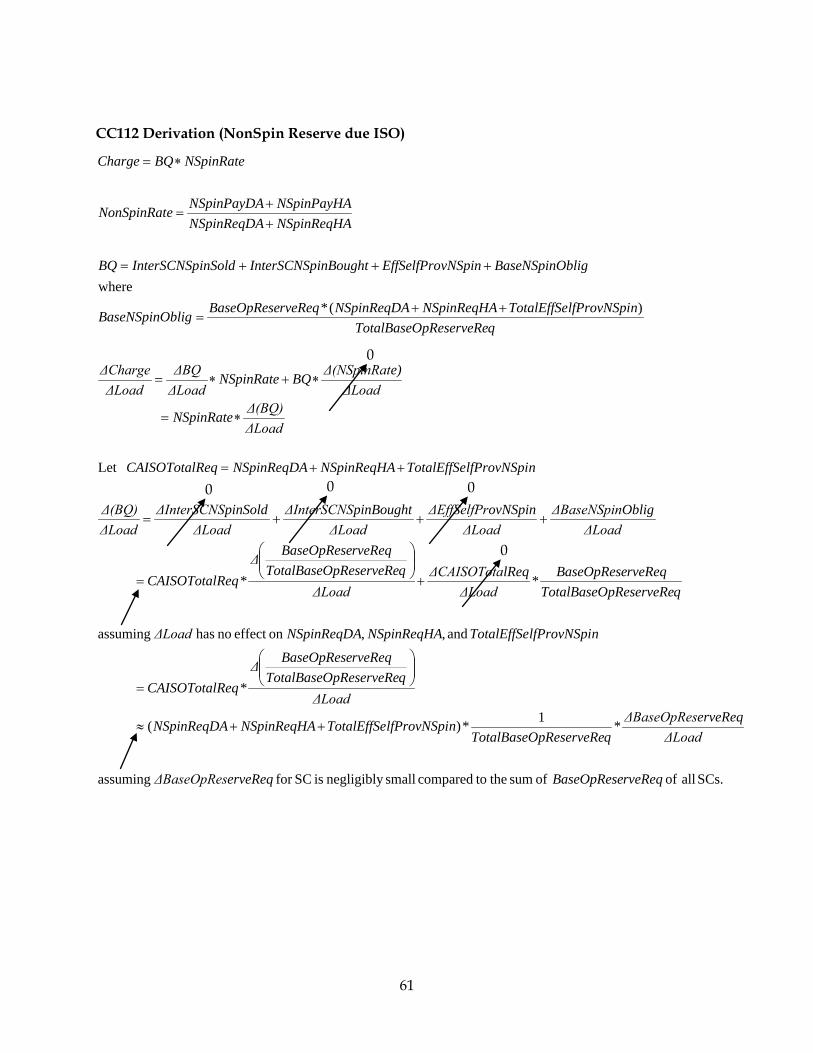
CC112 Derivation (NonSpin Reserve due ISO)

SCs. all of of sum the tocompared small negligibly is SCfor assuming

*1*)(

*

and,,on effect no has assuming

**

Let

)(*where

rveReqBaseOpReseerveReqΔBaseOpRes

ΔLoaderveReqΔBaseOpRes

qpReserveReTotalBaseOnlfProvNSpiTotalEffSeNSpinReqHANSpinReqDA

ΔLoadqpReserveReTotalBaseO

rveReqBaseOpReseΔReqCAISOTotal

nlfProvNSpiTotalEffSeNSpinReqHANSpinReqDAΔLoad

qpReserveReTotalBaseOrveReqBaseOpRese

ΔLoadlReqΔCAISOTota

ΔLoadqpReserveReTotalBaseO

rveReqBaseOpReseΔReqCAISOTotal

ΔLoadObligΔBaseNSpin

ΔLoadovNSpinΔEffSelfPr

ΔLoadpinBoughtΔInterSCNS

ΔLoadpinSoldΔInterSCNS

ΔLoadΔ(BQ)

nlfProvNSpiTotalEffSeNSpinReqHANSpinReqDAReqCAISOTotal

ΔLoadΔ(BQ)NSpinRate

ΔLoade)Δ(NSpinRatBQNSpinRate

ΔLoadΔBQ

ΔLoadΔCharge

qpReserveReTotalBaseOnlfProvNSpiTotalEffSeNSpinReqHANSpinReqDArveReqBaseOpResebligBaseNSpinO

bligBaseNSpinOvNSpinEffSelfProinBoughtInterSCNSpinSoldInterSCNSpBQ

NSpinReqHANSpinReqDANSpinPayHANSpinPayDAeNonSpinRat

NSpinRateBQCharge

++≈

=

+

=

+++=

++=

∗=

∗+∗=

++=

+++=

++

=

∗=

0

0 0 0

0

61

ΔLoaderveReqΔBaseOpRes

qpReserveReTotalBaseOqpReserveReTotalBaseOrveReqBaseOpRese

ΔLoadΔ

ΔLerveReqΔBaseOpRes

qpReserveReTotalBaseOLf

ΔLLff(L)

rveReqBaseOpReserveReqBaseOpReseerveReqΔBaseOpRes

rveReqBaseOpReserveReqBaseOpReserveReqBaseOpRese

rveReqBaseOpReseSCerveReqΔBaseOpRes

rveReqBaseOpReserveReqBaseOpReseerveReqΔBaseOpResrveReqBaseOpRese

rveReqBaseOpReseerveReqΔBaseOpResrveReqBaseOpReserveReqBaseOpReseerveReqΔBaseOpResrveReqBaseOpRese

Lf

ΔLLL

rveReqBaseOpReserveReqBaseOpReserveReqBaseOpRese

qpReserveReTotalBaseOrveReqBaseOpReseLf

Ni

i

Ni

i

Ni

ii

Niii

ii

Ni

i

SCSC

SC

SCSC

SC

i

SCSC

SCSC

SCSCSCSC

SCSC

SCSC

SC

*1

is,That

.*1)(' So

*)('

......

SCs. all of of sum the tocompared small negligibly is for assuming

...

......)'(

Then . 'let and

...)(let If

Since

11

1

1

1

≈

≈

+=

+++

++=

++

+≈

+++++

+=

+=

++==

Therefore,

( )Load

rveReqBaseOpReseqpReserveReTotalBaseO

nlfProvNSpiTotalEffSeNSpinReqHANSpinReqDANSpinRateLoad

Charge∆

∆∗

++≈

∆∆ *112

.Let ImportExportdMeteredLoaNetload −+=

then, If HydroNetload >=

( ) 07.0 *112 ∗

++≈

∆∆

qpReserveReTotalBaseOnlfProvNSpiTotalEffSeNSpinReqHANSpinReqDANSpinRate

LoadCharge

then, If HydroNetload <

( ) 05.0* 112 ∗

++≈

∆∆

qpReserveReTotalBaseOnlfProvNSpiTotalEffSeNSpinReqHANSpinReqDANSpinRate

LoadCharge

62

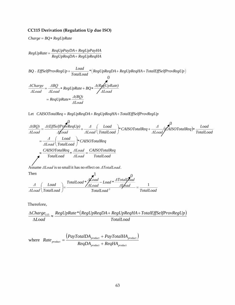
CC115 Derivation (Regulation Up due ISO)

( )

TotalLoadTotalLoadΔLoad

ΔTotalLoadLoadΔLoadΔLoadTotalLoad

TotalLoadLoad

ΔLoadΔ

ΔTotalLoadΔLoad

TotalLoadReqCAISOTotal

ΔLoadΔLoad

TotalLoadReqCAISOTotal

ReqCAISOTotalTotalLoad

LoadΔLoadΔ

TotalLoadLoadReqCAISOTotal

ΔLoadΔReqCAISOTotal

TotalLoadLoad

ΔLoadΔ

ΔLoadrovReqUp)Δ(EffSelfP

ΔLoadΔ(BQ)

plfProvRegUTotalEffSeRegUpReqHARegUpReqDAReqCAISOTotal

ΔLoadΔ(BQ)ReqUpRate

ΔLoade)Δ(RegUpRatBQRegUpRate

ΔLoadΔBQ

ΔLoadΔCharge

plfProvRegUTotalEffSeRegUpReqHARegUpReqDATotalLoad

LoadvRegUpEffSelfProBQ

RegUpReqHARegUpReqDARegUpPayHAReqUpPayDARegUpRate

RegUpRateBQCharge

1**

Then .on effect no hasit small so is Assume

*

*

Let

*

2 =−

=

=∗≈

=

∗+

+=

++=

∗=

∗+∗=

+++

++

=

∗=

=

Therefore,

( )TotalLoad

plfProvRegUTotalEffSeRegUpReqHARegUpReqDARegUpRateLoad

Charge ++≈

∆∆ *115

( )productproduct

productproductproduct ReqHAReqDA

PayTotalHAPayTotalDARate

+

+= where

0

0 0

0 1

63

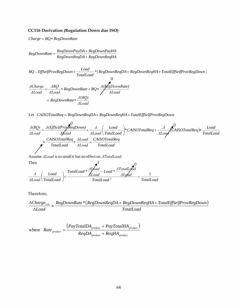
CC116 Derivation (Regulation Down due ISO)

( )

TotalLoadTotalLoadΔLoad

ΔTotalLoadLoadΔLoadΔLoadTotalLoad

TotalLoadLoad

ΔLoadΔ

ΔTotalLoadΔLoad

TotalLoadReqCAISOTotal

ΔLoadΔLoad

TotalLoadReqCAISOTotal

TotalLoadLoadReqCAISOTotal

ΔLoadΔReqCAISOTotal

TotalLoadLoad

ΔLoadΔ

ΔLoad)rovReqDownΔ(EffSelfP

ΔLoadΔ(BQ)

ownlfProvRegDTotalEffSeHARegDownReqDARegDownReqReqCAISOTotal

ΔLoadΔ(BQ)eReqDownRat

ΔLoadate)Δ(RegDownRBQeRegDownRat

ΔLoadΔBQ

ΔLoadΔCharge

ownlfProvRegDTotalEffSeHARegDownReqDARegDownReqTotalLoad

LoadvRegDownEffSelfProBQ

HARegDownReqDARegDownReqHARegDownPayDAReqDownPayeRegDownRat

eRegDownRatBQCharge

1**

Then .on effect no hasit small so is Assume

*

Let

*

2 =−

=

=∗≈

∗+

+=

++=

∗=

∗+∗=

+++

++

=

∗=

=

Therefore,

( )TotalLoad

ownlfProvRegDTotalEffSeHARegDownReqDARegDownReqeRegDownRatLoad

Charge ++≈

∆∆ *116

( )productproduct

productproductproduct ReqHAReqDA

PayTotalHAPayTotalDARate

+

+= where

0

0 0

0 1

64

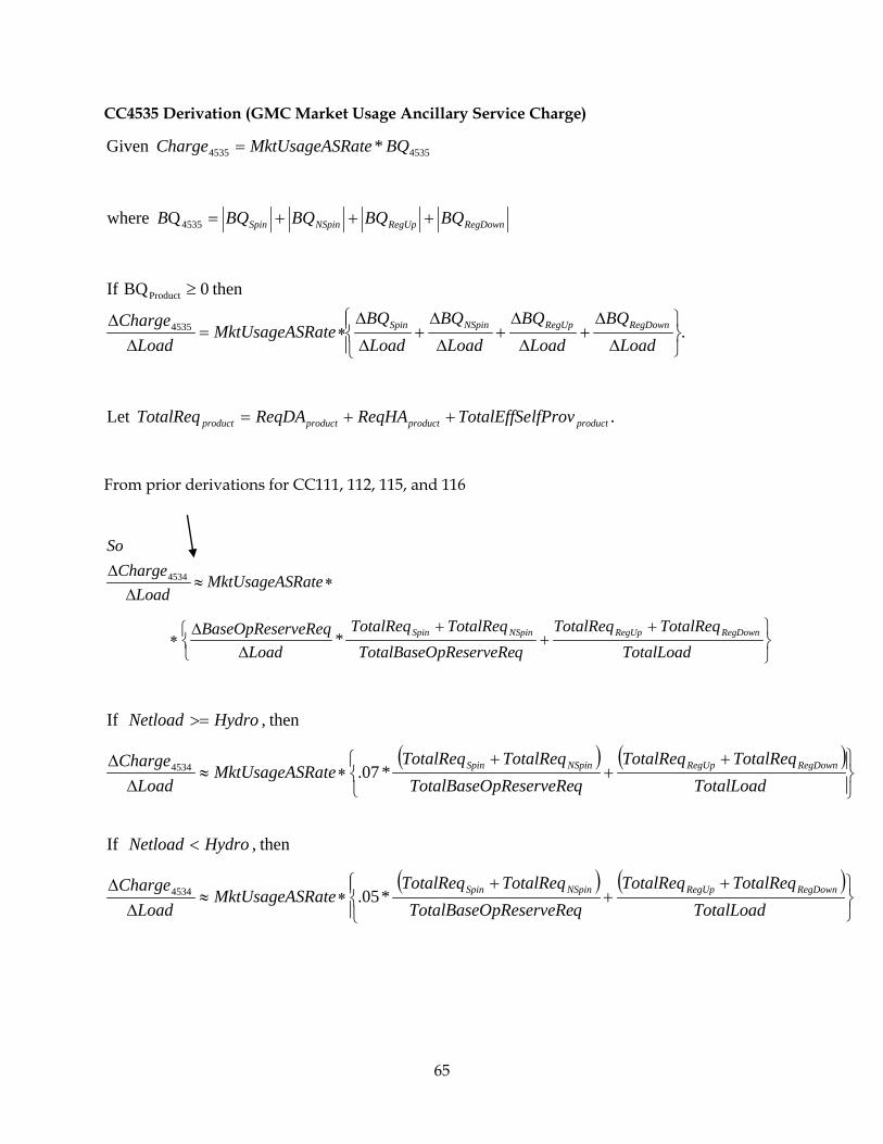
CC4535 Derivation (GMC Market Usage Ancillary Service Charge)

45354535 *Given BQRateMktUsageASCharge =

RegDownRegUpNSpinSpin BQBQBQBQB +++=4535Q where

.

then 0 BQ If

4535

Product

∆

∆+

∆

∆+

∆

∆+

∆

∆∗=

∆∆

≥

LoadBQ

LoadBQ

LoadBQ

LoadBQ

RateMktUsageASLoad

Charge RegDownRegUpNSpinSpin

.Let productproductproductproduct lfProvTotalEffSeReqHAReqDATotalReq ++=

From prior derivations for CC111, 112, 115, and 116

∗≈∆

∆RateMktUsageAS

LoadCharge

So

4534

+

++

∆∆

∗TotalLoad

TotalReqTotalReqqpReserveReTotalBaseO

TotalReqTotalReqLoad

rveReqBaseOpRese RegDownRegUpNSpinSpin *

then, If HydroNetload >=

( ) ( )

+

++

∗≈∆

∆TotalLoad

TotalReqTotalReqqpReserveReTotalBaseO

TotalReqTotalReqRateMktUsageAS

LoadCharge RegDownRegUpNSpinSpin

*07.4534

then, If HydroNetload <

( ) ( )

+

++

∗≈∆

∆TotalLoad

TotalReqTotalReqqpReserveReTotalBaseO

TotalReqTotalReqRateMktUsageAS

LoadCharge RegDownRegUpNSpinSpin

*05.4534

65

Appendix B-3: Requirements Specification

Summary Software Specification for Demand Response Trigger System (DR Triggers) Decision Support Tool

8/20/09

1. Overview

The requirements specification is based on requirements for the Demand Response Trigger Decision Support tool identified through a series of conference calls and meetings with Market Participants during July and August of 2009. Screen designs documented in the summary slides are included in this document, with further detail on how the graphic user interface should behave.

This document serves to provide more detailed functional descriptions considering the software development point of view. The document is divided into sections that detail the following:

1. Four GUI screens, although the prototype will be implemented for the first three. Namely, the screens are entitled: Day-Ahead, Day-Of, Configure and Scenario screens. The Scenario screen will not be considered in the prototype release, due to budget constraints for the prototype effort.

2. The Day-ahead and Day-of screens requires both the Trigger Impact calculations and the Resource portions of the screens in order to be considered complete and useful to the market participants.

3. The formula for ‘Ancillary Service’ for both ‘Day-Ahead’ and ‘Day-of’ will be made available in September. Although all work to be charged to the project must be completed before September 30, 2009, the drop dead date to receive the AS formulas is to be advised by the developer.

Rendering of ‘Imbalance Energy’ depends on user’s selection of ‘Select Mode’. If the user selects ‘Latest MRTU (for day-ahead)’ or ‘Latest MRTU Data (for day-of)’ then the application will download latest RT LMP data from MRTU OASIS for display (as detailed under the DA and Day-of screen specifications). Alternatively, if the user selects ‘Hourly Average Forecast’, then the application will read forecast data from a spread-sheet (to be provided by PG&E), and display the corresponding data matching date and selected location. The forecast file used in the ‘Day-Of’ screen represents day-of RT LMP forecasts and therefore is different from the Day-ahead RT LMP forecast file to be used in the ‘Day-Ahead’ screen. Note: Both files and their locations are user-specified via the Configure screen.

4. The rendering of ‘GMC in both ‘Day-Ahead’ and ‘Day-of’ in the current release (prototype) will use a mocked-up data instead of live data feeds. The mocked up data for GMC (shown on the screens) is a small value compared to Imbalance Energy and Ancillary Service values shown on the screens for Trigger Impact. The mocked up data is expected to be relatively constant between time intervals.

66

5. The rendering of ‘Total-Impact’ will take the sum of ‘Imbalance Energy’, ‘Ancillary Service’ and ‘GMC’ and display in the same column.

6. Rendering of data under ‘Resource Name’ in both ‘Day-Ahead’ and ‘Day-Of’ will be based on the DR Program Cost files (provided by PG&E) for ‘Day-Ahead’ and ‘Day-Of’ program resource costs and MW availability, respectively. (Further details on rendering of the Resource Cost section of the screen in given under the “Day Ahead” and “Day-of” screen subsections).

2. Target User and Functions beyond Status Quo

The target user of the decision support tool is short-term procurement personnel from the day-ahead and day-of desks. The new functionality provided by the specified tool is the capability of computing Trigger Impact by charge category. This is shown in the upper half of the Day-ahead and Day-of screens. Currently, market participants consider market price (i.e., supply alternatives from bilateral counterparties or the ISO) weighed against demand response program resource costs. Therefore, the target user currently has the DR program cost and MW availability information (shown on the bottom half of the DA and Day-of screens). Beyond current capabilities, the DR Trigger System Decision Support tool enables short-term procurement personnel to compare the DR Program Resource Costs with the impact of triggering each MW of demand response on wholesale settlements for the analyzed charge categories. In order words, the user is empowered for the first time with information on charges that can be avoided/reduced on wholesale settlements from “self-supply” of procurement short-falls (below daily demand forecasts) using demand response resources. The combination of being equipped with Trigger Impact information plus the ability to compare against DR Program Resource Costs provides new information to the user in support of day-ahead and day-of decision-making on triggering demand response (e.g., which resource, how much, and when to trigger).

67

3. Day-Ahead Screen

Picture 3-1

At application start, all the “green” cells will be blank, until user selects a location on ‘Select: Location’ pull down and selects a mode under ‘Select: Mode’, and clicks the button ‘Update’.

At the bottom of the screen are the controlling knobs and switches.

The ‘Select: Location’ pull down will display the ‘selectable locations’ that are similar to the ‘Default Locations’ described in the ‘Configuration’ Screen. The difference is a single selected location specifies the location (used after the user clicks the ‘Update’ button) for all the Trigger Impact Calculations: ‘Imbalance Energy’, ‘Ancillary Service’, ‘GMC’.

The ‘Select: Mode’ control the way of retrieval and displaying the data to the rows under ‘Charge Category’. All items under the ‘Resource Name’ will be filtered by the selected location-code/location-name, and displayed as soon as the user selects a location from the ‘Select: Location’ pull down.

For ‘Imbalance Energy’, if the user clicks on ‘Latest MRTU Data’, the application will download latest MRTU Data from CAISO web service relevant to the Trigger Impact calculations. For the matching location-code data, RT LMP data will be displayed on the Imbalance Energy line. If the user clicks on the ‘Hourly Forecasts’ mode, then data will be displayed from a Day-ahead RT LMP forecast file.

68

3.1 Render the RT LMP data for ‘Imbalance Energy’ row under “Latest MRTU Data” mode.

If user selects the ‘Latest MRTU’ data, the application will download RT LMP data from CAISO MRTU site, retrieving data and rendering them on the row for ‘Imbalance Energy’ in the ‘Day Ahead’ screen.

The application downloads ‘Interval Locational Marginal Price (ILMP)’ for the current date and yesterday’s date for the selected location. ‘Select node’ or select location as specified in the Configuration (be default) can be changed by the user’s selection for ‘Location’ in the Day-ahead screen. Note: although not necessary for this particular render function, the application would also download ILMP for each desired SLAP and DLAP location shown in the DR Program Cost file (e.g., PGE_DLAP, SCE_DLAP, SDGE_DLAP), in order to populate the output file resulting from the ‘Update’ function.

Specify both the ‘Date From’ and ‘To’ to today’s date and specify the Hours to be downloaded, then click the button ‘CSV download’. Each hour of data will have 12 (5 minutely) interval data values. The application takes the average of the 12 (5 minutely) interval data values to calculate the hourly average RT LMP. All 12 interval values (zero and-non zero) will be used to compute the hourly average RT LMP.

For example, if the ‘update’ button is clicked at 15:10 (3:10 PM) of a given day, then it will download/display the hourly average for the hours 1-14 of the same day, but display the hourly average data of hour 15-24 of previous day, and populate these values into the ‘HE1 – HE24’ cells of ‘Imbalance Energy’ line.

The downloaded file is assumed to be in zipped format, so will be unzipped to a CSV formatted file, then read by the application. A sample downloaded CSV file has the following appearance:

Picture 3-3

The application will select only the rows with matching value of ‘LMP’ in column G (LMP Type), and matching location code (for example, ‘SLAP_PGEB-APND’ in column E (Node) – only single row will be selected), and take the values of column L (INTERVAL01) to column W (INTERVAL12). The Hour value will be in the Column B (OPR_HR). The application will take all existing values among INTERVAL01 and INTERVAL12, sum and average against existing field-count as the hourly forecast cost.

69

3.2 Render data for ‘Imbalance Energy’ with Select Mode = ‘Hourly Forecast’

The values to display are from the file specified in the field ‘DA Forecasts’ under the ‘Configure’ Screen.

3.3 Render data for ‘Ancillary Service’ with Select Mode = “Latest MRTU Data”

TBD

3.4 Render the ‘Ancillary Service’ with Select Mode = ‘Hourly Forecast’

The input data file comes from the file specified in field ‘DA Forecasts’ field in ‘Configure’ Screen.

3.5 Render data for ‘GMC’ row with Select Mode = “Latest MRTU Data”

In the prototype release, the GMC will be retrieved from a mock-up data file, the input file is defined in the ‘Sample MRTU Data’ field of the ‘Configure’ screen.

3.6 Render the ‘GMC’ row data with Select Mode = ‘Hourly Forecast’

The input data file comes from the file specified in field ‘DA Forecasts’ field in ‘Configure’ Screen.

3.7 Render rows under ‘Resource Name’

In terms of priority, rendering of this portion will be next to the rendering for ‘Imbalance Energy’, and before ‘Ancillary Service’.

The data rendered under the ‘Day-Ahead’ screen will be from the input data file specified under the ‘DR Program Costs’ field of the ‘Configure’ Screen.

70

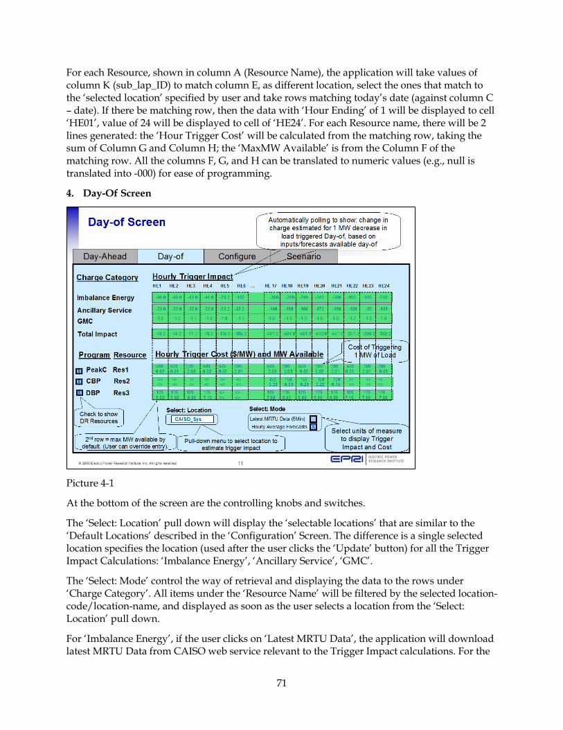
For each Resource, shown in column A (Resource Name), the application will take values of column K (sub_lap_ID) to match column E, as different location, select the ones that match to the ‘selected location’ specified by user and take rows matching today’s date (against column C – date). If there be matching row, then the data with ‘Hour Ending’ of 1 will be displayed to cell ‘HE01’, value of 24 will be displayed to cell of ‘HE24’. For each Resource name, there will be 2 lines generated: the ‘Hour Trigger Cost’ will be calculated from the matching row, taking the sum of Column G and Column H; the ‘MaxMW Available’ is from the Column F of the matching row. All the columns F, G, and H can be translated to numeric values (e.g., null is translated into -000) for ease of programming.

4. Day-Of Screen

Picture 4-1

At the bottom of the screen are the controlling knobs and switches.

The ‘Select: Location’ pull down will display the ‘selectable locations’ that are similar to the ‘Default Locations’ described in the ‘Configuration’ Screen. The difference is a single selected location specifies the location (used after the user clicks the ‘Update’ button) for all the Trigger Impact Calculations: ‘Imbalance Energy’, ‘Ancillary Service’, ‘GMC’.

The ‘Select: Mode’ control the way of retrieval and displaying the data to the rows under ‘Charge Category’. All items under the ‘Resource Name’ will be filtered by the selected location-code/location-name, and displayed as soon as the user selects a location from the ‘Select: Location’ pull down.

For ‘Imbalance Energy’, if the user clicks on ‘Latest MRTU Data’, the application will download latest MRTU Data from CAISO web service relevant to the Trigger Impact calculations. For the

71

matching location-code data, RT LMP data will be displayed on the Imbalance Energy line. If the user clicks on the ‘Hourly Forecasts’ mode, then data will be displayed from a Day-of RT LMP forecast file.

Although the screen designs are almost identical, the major difference of this screen and the ‘Day-Ahead’ screen include the following functions:

• automatic polling in the Day-of screen

• different RT LMP forecast files to use in each screen, since the DA screen uses DA forecasts and the other uses Day-of forecasts of the RT LMPs

• different DR program cost files to use in each screen

• the Day-of Screen shows the latest 5minute RT LMP for current hour-ending (HE) interval on day-of screen's imbalance energy line, when Latest MRTU Data mode is selected. That is for the current HE interval, the application shows in the DA screen the previous day's value for the same interval as the current interval. However, the application shows the latest day-of 5min RT LMP in the Day-of screen for the current HE interval. Note: for the DA screen, the current HE interval is defined to be the HE interval that the user clicks the ‘Update’ button on the DA Screen.

Under the ‘Select: Mode’, if ‘Latest MRTU Data (5 min)’ selected, then this screen will retrieve the latest MRTU data for RT LMP every 5 minutes, and refresh the screen.

Under the ‘Select: Mode’, if ‘Hourly Average Forecasts’ selected, then the application will load file defined in the ‘Day-of Forecasts:’ field in the ‘Configure’ Screen.

For example, if the current HE cell is HE15 (at 15:10 (3;10PM), the ‘Day of’ screen will show downloaded ILMP (refer to Picture 3-2) for the current HE interval. Despite whether or not the 12 intervals might not be available in the middle-of-the-hour, the application will display the current RT ILMP in the current HE cell. Average hourly ILMP is computed and shown for the other HE cells.

4.1 Render the OASIS-MRTU data for ‘Imbalance Energy’ row

The rendering of OASIS_MRTU data for ‘Imbalance Energy’ row for ‘Day-of’ is the same as the rendering of OASIS-MRTU data for ‘Imbalance Energy’ row for ‘Day-Ahead’.

Please refer to section 3.1.

4.2 Render the ‘Imbalance Energy’ row data with Select Mode = ‘Hourly Forecast’

The input data file comes from the file specified in field ‘Day-of Forecasts’ field of the ‘Configure’ Screen.

4.3 Render the ‘Ancillary Service’ with Select Mode = ‘Latest MRTU Data’

TBD

72

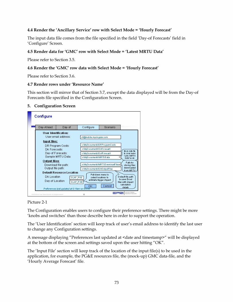
4.4 Render the ‘Ancillary Service’ row with Select Mode = ‘Hourly Forecast’

The input data file comes from the file specified in the field ‘Day-of Forecasts’ field in ‘Configure’ Screen.

4.5 Render data for ‘GMC’ row with Select Mode = ‘Latest MRTU Data’

Please refer to Section 3.5.

4.6 Render the ‘GMC’ row data with Select Mode = ‘Hourly Forecast’

Please refer to Section 3.6.

4.7 Render rows under ‘Resource Name’

This section will mirror that of Section 3.7, except the data displayed will be from the Day-of Forecasts file specified in the Configuration Screen.

5. Configuration Screen

Picture 2-1

The Configuration enables users to configure their preference settings. There might be more ‘knobs and switches’ than those describe here in order to support the operation.

The ‘User Identification’ section will keep track of user’s email address to identify the last user to change any Configuration settings.

A message displaying “Preferences last updated at <date and timestamp>“ will be displayed at the bottom of the screen and settings saved upon the user hitting “OK”.

The ‘Input File’ section will keep track of the location of the input file(s) to be used in the application, for example, the PG&E resources file, the (mock-up) GMC data-file, and the ‘Hourly Average Forecast’ file.

73

DR Program Costs File:

The ‘DR Program Costs’ will be used to store the data under ‘Resource Name’ (what the ‘Function B’ refer to in the power-point slides). The name of the resource will come from column A, each resource will have two lines of data displayed – the ‘Hourly Trigger Cost’ is the sum of Column G and Column H; the second line will be he ‘MaxMW Available come from Column F of the file. Column G, H, and F must have numeric only data – space, null or other non-numeric value will cause application fail to read the data.

DA Forecasts:

If user click the ‘Hour Forecasts’ in the ‘Day-Ahead’ screen, then the ‘Imbalance Energy’, ‘Ancillary Service’ and ‘GMC’ will be read from the ‘DA Forecasts’ file. The file will be defined in the field ‘DA Forecasts’ of the ‘Configuration’ Screen.

Day-of Forecasts:

If user click the ‘Hourly Average Forecasts’ in the ‘Day-of’ screen, then the ‘Imbalance Energy’, ‘Ancillary Service’ and ‘GMC’ will be read from the ‘Day-of Forecasts’ file. The file will be defined in the field ‘Day-of Forecasts’ of the ‘Configuration’ Screen.

The ‘Output files’ will store the directory path for output the export file (when user request to output the data in excel/csv format).

Download file path:

The ‘Download file path’ field in the Configure Screen will keep track of the directory-path used for download file from OASIS-MRTU web service. The default directory is ‘C:\Temp\OASIS’ directory. Under the path, the sub-directory ‘download’ will store all the original downloaded files (in zip format), after download the zipped file, the application will try to un-zip the file and store them into the sub-directory ‘result’. If user do not change the default setting, then the raw data will be downloaded to ‘C:\temp\OASIS\download’, and the final un-zipped files will be in ‘C:\temp\OASIS\result’ directory.

Output File Path:

The ‘Output File Path’ field in the Configure Screen will keep track of the file-path used for the ‘Update’ function. In the ‘Day-Ahead’ Screen, when user click the ‘Update’ button, it will do the download (or read file), then populate all locations of data into the excel files defined in this field.

Default Resource Location:

Store the default location set by user. When user start the application, the default location for that screen will be selected. The selectable locations are from the ‘DR Program Costs:’ file. Figure 2-2 is from an old version of file. The selectable location data come from column K, L, M, N (column N is not available in the old release of file).

DA Location:

The default location for the ‘Day Ahead’ screen.

74

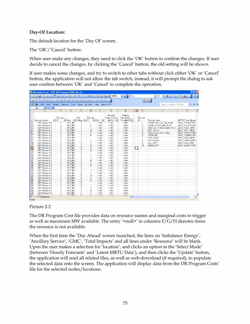
Day-Of Location:

The default location for the ‘Day Of’ screen.

The ‘OK’/’Cancel’ button:

When user make any changes, they need to click the ‘OK’ button to confirm the changes. If user decide to cancel the changes, by clicking the ‘Cancel’ button, the old setting will be shown.

If user makes some changes, and try to switch to other tabs without click either ‘OK’ or ‘Cancel’ button, the application will not allow the tab switch, instead, it will prompt the dialog to ask user confirm between ‘OK’ and ‘Cancel’ to complete the operation.

Picture 2-2

The DR Program Cost file provides data on resource names and marginal costs to trigger as well as maximum MW available. The entry ‘<null>’ in columns F/G/H denotes times the resource is not available.

When the first time the ‘Day Ahead’ screen launched, the lines on ‘Imbalance Energy’, ‘Ancillary Service’, ‘GMC’, ‘Total Impacts’ and all lines under ‘Resource’ will be blank. Upon the user makes a selection for ‘location’, and clicks an option in the ‘Select Mode’ (between ‘Hourly Forecasts’ and ‘Latest MRTU Data’), and then clicks the ‘Update’ button, the application will read all related files, as well as web-download (if required), to populate the selected data onto the screen. The application will display data from the DR Program Costs’ file for the selected nodes/locations.

75

6. Scenario Screen

Functions supported by Scenario screen include:

A. In addition to information shown on DA/Day-of screens, also show hourly Market Price (from datafile) below Total Impact calculations

B. Allow user to define each of two Scenarios to compare by configuring for each:

1*. Name of Resources in the scenario – selected using a pull down menu of resources

2. MW quantity of resource – through user-override of default max MW available values that show in the white rows

C. Compute and show Net result for each user-defined resource scenario per:

1. Include in Net calculation the HE intervals with radio buttons clicked for resources that are checked

2. Include in Net calculation the resources that are checked

3. Compute Net for each HE interval as:

Net = SumoverselectedDRResources{(TotalImpact+DRProgramCost)*MW_DRResource}

+ SumoverselectedMarketResources{(MarketPrice*MW_MktResource)}

76

D. Compute and show Difference of Net impact for the two user-defined Resource Scenarios per:

Difference = Net1 – Net2

E. Perform Net and Difference calculations based on user selection of

1. DA or Day-of radio button – to select the context (and data) for scenario comparison

2. Location – to select location of resources that will show on pull-down menu of resources, and that will determine the location for the Hourly Trigger Impact calculations

* Denotes optional feature

77

Appendix B-4: Published Contribution The following contribution by the principal investigator was published in the Proceedings of the 2008 CIGRE Paris Session. The contribution provides a response to the question noted below.

Question 1.7

Can utilities comment on the level of adoption of various DSI implementation strategies? Are there practical examples where information signal are used to coordinate demand response with market conditions? What types of trigger signals are being used or are under development?

Title:

Trigger Signals and Adoption Levels of Demand Response Programs in the U.S.

Collectively, Demand-side Integration (DSI) efforts focus on advancing the efficiency and effective use of electricity in support of power systems and customer needs [1] [2]. CIGRE Working Group C6.09 has adopted this term to refer to “the overall technical area focused on the demand-side and its potential as a source of supply, including demand response and energy efficiency.” [3] After initial proposal through the author’s spontaneous contribution at the CIGRE General Session in 2006 and subsequent adoption by the working group, there has been growing recognition of Demand-side Integration as the underlying technical issue encompassing all aspects of demand-side management in today’s restructured industry environment [2][3][4][5].

The subject of trigger signals pertains to DSI implementations focused on achieving demand response. Adoption levels for demand response programs in the U.S. are indicated in Figure 23. The total peak reduction potential was approximately 30GW, based on a survey published in 2006 by the Federal Energy Regulatory Commission (FERC). Given a total peak demand of roughly 750GW, the U.S. adoption level was about 4% at the time of the survey.

78

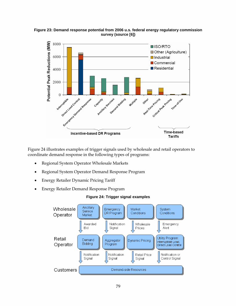
Figure 23: Demand response potential from 2006 u.s. federal energy regulatory commission survey (source [6])

Figure 24 illustrates examples of trigger signals used by wholesale and retail operators to coordinate demand response in the following types of programs:

• Regional System Operator Wholesale Markets

• Regional System Operator Demand Response Program

• Energy Retailer Dynamic Pricing Tariff

• Energy Retailer Demand Response Program

Figure 24: Trigger signal examples

79

Choice of trigger signals utilized by wholesale and retail operators, respectively, varies by demand response program and depends on the program’s defined actuation method. The actuation method dictates information exchange requirements of the particular program, for which the trigger signal is one aspect.

As described in [2] and [4], a demand response program’s actuation method specifies the

i) actuator or entity responsible for actuating a response, and

ii) choice of trigger or type of information signal used to coordinate demand response with system or market conditions.

Practical examples of actuation methods include:

• Customer-actuated response to notification signals

• Operator-actuated response via automated controls

• Customer-actuated response to price signals

References:

1. Advancing the Efficiency of Electricity Utilization-”Prices to DevicesTM”: Background Paper, 2006 EPRI Summer Seminar. EPRI, Palo Alto, CA. Available at http://www.epri.com.

2. A.S., Chuang, “Demand-side Integration for System Reliability”, Proceedings of PowerTech, Lausanne, July 1-5, 2007, pp.1617-1622.

3. A. Baitch, A. Chuang, G. Mauri, C. Schwaegerl, “International Perspectives on Demand-side Integration”, Proceedings of the 19th International Conference on Electricity Distribution (CIRED), Vienna, May 21-24, 2007.

4. A.S. Chuang, C.W. Gelling, “Demand-side Integration in a Restructured Electric Power Industry”, CIGRE General Session, Paris, France, August 24-29, 2008.

5. TSOLID-DER, “Co-ordination Action to Consolidate RTD Activities for Large-scale Integration of DER into the European Electricity Market”, 2006, Deliverable D2.1, Work Package II, Task 2.3; Project co-funded by the European Commission within the Sixth Framework Programme (2002-2006). Available at http://www.solid-der.org.

6. “Assessment of Demand Response and Advanced Metering”, Staff Report, Federal Energy Regulatory Commission, Docket AD-06-2-000, August 2006.

80

APPENDIX P Appendix P: Appendix 9: Privacy in the Smart Grid: An Information Flow Analysis

2087 Addison Street, 2nd Floor Berkeley, CA 94704-110

(510) 643-1440 uc-ciee.org

California Institute forEnergy and Environment

Privacy in the Smart Grid: An Information Flow Analysis

Final Project Report March, 2011 Prepared by UC Berkeley School of Information, University of California, Berkeley Prepared for CIEE Enabling Technologies Development Program Program Manager Gaymond Yee

5

CHAPTER 1: Introduction 1.1 Background In the century since residential electrical service started to become a ubiquitous feature of life in the United States, the details of how households consume electricity have largely remained inside the home. Electromechanical meters have kept track of total electricity usage, revealing little more than an aggregated figure summarizing how much electricity a household used since the last meter reading. These meters did not record or reveal who used electricity, when, or where, nor did they allow energy consumption to be noted in real-time.

All of this is changing as digital “smart meters” become part of California’s (and the nation’s) energy infrastructure. Smart meters, as components of the advanced metering infrastructure (AMI), serve a broader effort to construct a “Smart Grid” by integrating information technology into electricity generation, transmission, and distribution. According to the Federal Energy Regulatory Commission (FERC), as of September 2009, there were approximately eight million advanced meters installed nationwide; FERC expects that number to reach 80 to 141 million by 2019.5 In California, the three major investor-owned utilities (IOUs) are in the midst of deploying smart meters for electricity; they plan to deploy approximately 12 million electric meters by the end of 2012.6

Concurrent with this evolution in metering is the development of home area networks (HAN) composed of devices that communicate with one another and can communicate data to utilities (or other energy service providers) and can receive and respond to signals sent by these remote entities. An overarching vision of the Smart Grid holds that providing consumers with information about their energy usage will support an array of electricity pricing models and enable customers to better control their electricity use (or authorize a third party to do so).7

5 Federal Energy Regulatory Commission, Assessment of Demand Response and Advanced Metering (Staff Report) (Sept. 2009), http://www.ferc.gov/legal/staff-reports/sep-09-demand-response.pdf (last visited June 19, 2010).

6 KEMA, Final Report for the Meter and Market Assessment Project 8-20-8-21 (Aug. 2009), http://www.cpuc.ca.gov/NR/rdonlyres/F83E3AA1-7049-4C33-A720-1A3215F4A300/0/CSISolarMeteringReport_Final8409.pdf (last visited June 19, 2010). Pacific Gas & Electric and San Diego Gas & Electric are also deploying smart gas meters. Id. at 8-20. This report, however, focuses on electric meters.

7 See Energy Independence and Security Act of 2007 (EISA) § 1306, Pub. L. 110-140 (codified at 42 U.S.C. §§ 17001 et seq.); Senate Bill 17 (Padilla, Chapter 327, Statutes of 2009) (codified at CAL. PUB. UTILS. CODE § 8360 et seq.). See also P.A. Subrahmanyam, David Wagner, Deirdre Mulligan, Erin Jones, Umesh Shankar, and Jack Lerner, Network Security Architecture for Demand Response/Sensor Networks 43 (June 2006) (stating that two-way information flows between consumers and utilities or service providers have “the potential to enable a variety of advanced utility applications; such as demand response, energy management services, improved outage management, automation functions, advanced metering and reporting, power quality management, and many other functions”) [CyberKnowledge/Berkeley Report].

6

Many details of the architecture(s) that will connect individuals to the Smart Grid, however, remain to be decided.

One end of the design spectrum would rely largely on one-way transmissions of price and event information to customers; energy management systems within customers’ homes or businesses would then control networked devices based on these signals and the customer’s preferences.

At the other end of the spectrum is a Smart Grid that depends on two-way communications between home devices and utilities or other service providers. In this two-way architecture, a home area network (HAN) gateway8 enables not only communications between devices inside the home and service providers but also remote control of HAN devices . Other architectures are feasible, too. One-way broadcast transmissions of day-ahead price information, for example, have shown promise to achieve significant shifts away from peak demand.

The California Public Utilities Commission has chosen to promote technologies and business models that embrace intensive two-way communications. The CPUC approved utilities’ requests to include HAN gateways in their smart meter deployments. The CPUC reasoned that doing so would provide “[t]he most cost effective way . . . over the long term” of realizing the benefits of “enabling price signals, load control and near real time data for residential electric customers.”9 Given the combined size of the major California IOUs’ deployments and California’s advanced state of Smart Grid activity relative to other states, these decisions are likely to influence other states. Federal policy could provide additional support to this influence. The U.S. Department of Energy, for example, is promoting a bi-directional communications model on the grounds that it will allow individuals and businesses to contribute electricity to the grid and respond to dynamic electricity prices.10

But the highly detailed usage and control data that smart meters and HAN gateways transmit also create risks for individual privacy. Instead of providing one data point per month directly to a utility, as was the case with electromechanical meter depicted in Figure 1, the smart meters currently being deployed in California will send hourly readings—hundreds per month—to utilities; and they are capable of taking readings every few seconds for a near-real-time picture of energy consumption.11

8 Some sources refer to the HAN gateway as an “electric services interface” (ESI). These two phrases have the same meaning. For consistency, we use HAN gateway throughout this report.

9 Decision on Pacific Gas and Electric Company’s Proposed Upgrade to the SmartMeter Program 176-77, CPUC A.07-12-009 (Mar. 12, 2009).

10 Dept. of Energy, Smart Grid System Report 14-16 (July 2009). The Department of Energy has developed its own Smart Grid privacy analysis. See U.S. Department of Energy, Data Access and Privacy Issues Related to Smart Grid Technologies, Oct. 5, 2010, http://www.gc.energy.gov/documents/Broadband_Report_Data_Privacy_10_5.pdf.

11 See Decision Adopting Policies and Findings Pursuant to the Smart Grid Policies Established by the Energy Information [sic] and Security Act of 2007 78, CPUC R.08-12-009 (Dec. 29, 2009) (ordering the three major IOUs in California to “provide to their customers with a smart meter access to usage data on a real-time or near real-time basis no later than the end of 2011”); Southern California Edison’s (U-338-E) Reply Comments to Assigned Commissioner and Administrative Law Judge’s Joint Ruling Amending

7

The CPUC currently plans to order the three major IOUs to provide customers and authorized third parties with “near real time” access to energy usage data by the end of 2011.12 Other states may follow California’s example.

This fine-grained data reveals much more than mere electricity consumption: it can reveal when the occupants of a residence are awake or asleep, at home or away.13 In addition, data from HAN devices can provide distinct data streams that reveal exactly what devices a customer used and when the customer used a given device. Put simply, smart meters currently being deployed offer a direct view into household activities. The clarity of this view will increase as devices connected on home area networks begin to provide more specific usage information and identifiers tied to specific devices.

Figure 1: Pre-Smart Grid Model: Meter data flow from electromechanical meter to utility.

Electromechanical meters measure aggregate electricity consumption at a customer’s premises. Utilities read these meters once per month to bill customers for their electricity use. Data flows simply from the home to the utility, the blue building that shows that electricity may come from any of a variety of sources (solar, coal, wind, nuclear, etc.). Graphics Credit: Brian P. Miller Photo & Design, http://www.brianpmillerphotography.com/

The privacy risks arising from smart meter and HAN device data are legion.14 Utilities may seek to monetize the information they collect from smart meters.15 Likewise, third parties may use

Scoping Memo and Inviting Comments on Proposed Policies and Findings Pertaining to the Smart Grid 14, CPUC R.08-12-009 (Apr. 7, 2010) (“SCE, PG&E, and SDG&E have plans to provide near real-time usage data, in approximately ten-second increments, to all residential customers.”). All documents filed in this CPUC rulemaking ate available at http://docs.cpuc.ca.gov/Published/proceedings/R0812009_doc.htm.

12 Decision Adopting Policies and Findings Pursuant to the Smart Grid Policies Established by the Energy Information [sic] and Security Act of 2007, D.09-12-046, at 77 (Dec. 17, 2009).

13 See Mikhail A. Lisovich, Deirdre K. Mulligan, and Stephen B. Wicker, Inferring Personal Information from Demand Response Systems, IEEE SECURITY & PRIVACY, Jan./Feb. 2010, 11-20; Elias Leake Quinn, Smart Metering & Privacy: Existing Law and Competing Policies (Spring 2009).

14 For a list of risks—including identity theft, real-time surveillance, home invasions, stalking and domestic Abuse–generated by the NIST Privacy Subgroup see Draft slides submitted for use by NIST at Grid Interop November 2009, available at: http://collaborate.nist.gov/twiki-sggrid/bin/view/SmartGrid/CSCTGPrivacy (last checked on November 22, 2010).

8

this data to market products and services.16 In the wrong hands, this data about electricity usage may indicate when a home is occupied, exposing people and property to potential harm.

Finally, legal privacy protections for utility records were developed around relatively unrevealing data—monthly aggregate consumption, as mentioned above. Going forward, utility records will contain vastly more detailed data generated by interactions with the Smart Grid. The detailed data will make utility records a more attractive investigative tool, thus encouraging access requests by law enforcement agents and litigants in civil lawsuits, such as divorce proceedings. An analogy may be found in the use of cell phone calling records to obtain location information about criminal suspects: the steady increase in the use of cell phones has been accompanied by increasingly dense communications infrastructure that provides increasingly accurate information about a phone’s location. 17 These factors have made cell phone location information an increasingly rich tool for law enforcement investigations, though many cell phone users are unaware that their providers have historic data about their location as well as the ability to track them in real-time.18 Courts and Congress have been slow to adopt or expand rules to regulate law enforcement access to this increasingly sensitive information.19

Moreover, Smart Grid data20 privacy is not an isolated issue. The details of how data flows from meters to customers, utilities, and third parties (and vice versa) also raise several concerns about grid cybersecurity and its openness to innovation, including:

15 Southern California Edison (SCE), SmartConnect Use Case: C7 – Utility Uses SmartConnect Data for Targeted Marketing Campaigns, http://www.sce.com/NR/rdonlyres/E2927535-15B3-41F3-AE88-B06CE760225F/0/C7_Use_Case_081229.pdf

16 Southern California Edison (SCE), SmartConnect Use Case: C7 – Utility Uses SmartConnect Data for Targeted Marketing Campaigns, http://www.sce.com/NR/rdonlyres/E2927535-15B3-41F3-AE88-B06CE760225F/0/C7_Use_Case_081229.pdf.

17 The rapid growth in the popularity of cell phones, the continuing deployment of cell phone infrastructure, and advances in phone-based geolocation technologies (e.g., GPS), have made location information possessed by cell phone service providers an increasingly used—and useful—tool for law enforcement investigations. See In re Application of the United States of America for an Order Directing a Provider of Electronic Communications Service to Disclose Records to the Government, No. 07-524M, slip. op. at 8-10 (W.D. Pa., Feb. 19, 2008) (noting ten-fold growth in number of U.S. cell phone users from 1994 to 2006 and ability of cell service providers to localize a phone to a 200-foot radius in some areas).

18 Id. at 3 (stating that cell site location information is “broadly sought” by law enforcement agencies).

19 See id. at 10-23 (reviewing relevant laws). Still, the law does evolve. For example, the U.S. Court of Appeals for the D.C. Circuit recently held that police tracking of all of a suspect’s movements over the course of a month via GPS was a search subject to the Fourth Amendment’s reasonableness requirements. United States v. Maynard, No. 08-3030, slip op. at 16-34 (D.C. Cir., Aug. 3, 2010). The court noted that, while many movements are exposed to the public, “prolonged GPS monitoring reveals an intimate picture of the subject’s life that he expects no one to have—short perhaps of his spouse.” Id. at 32. But see also United States v. Pineda-Moreno, No. 08-30385 (9th Cir., Jan. 11, 2010) (holding that police use of a mobile tracking device on a suspect’s car was not a search at all).

20 We use “Smart Grid data” as an umbrella terms that refers to information pertaining to residential customers’ electricity usage. As discussed in more detail in Chapter 3, this data includes consumption data, price information, and HAN device control traffic.

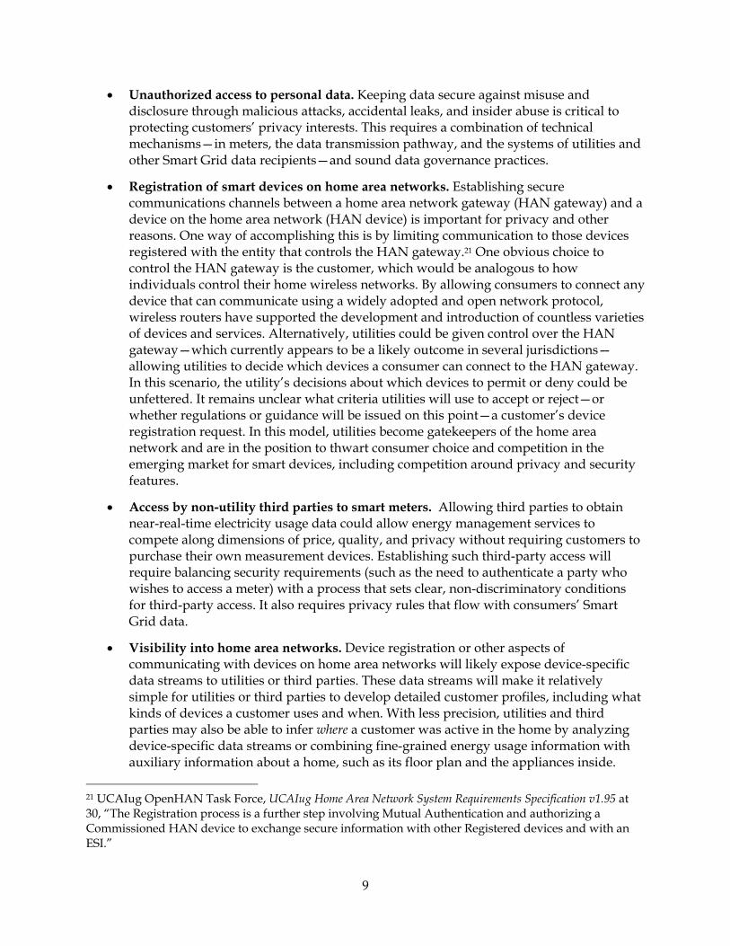
9

Unauthorized access to personal data. Keeping data secure against misuse and disclosure through malicious attacks, accidental leaks, and insider abuse is critical to protecting customers’ privacy interests. This requires a combination of technical mechanisms—in meters, the data transmission pathway, and the systems of utilities and other Smart Grid data recipients—and sound data governance practices.

Registration of smart devices on home area networks. Establishing secure communications channels between a home area network gateway (HAN gateway) and a device on the home area network (HAN device) is important for privacy and other reasons. One way of accomplishing this is by limiting communication to those devices registered with the entity that controls the HAN gateway.21 One obvious choice to control the HAN gateway is the customer, which would be analogous to how individuals control their home wireless networks. By allowing consumers to connect any device that can communicate using a widely adopted and open network protocol, wireless routers have supported the development and introduction of countless varieties of devices and services. Alternatively, utilities could be given control over the HAN gateway—which currently appears to be a likely outcome in several jurisdictions—allowing utilities to decide which devices a consumer can connect to the HAN gateway. In this scenario, the utility’s decisions about which devices to permit or deny could be unfettered. It remains unclear what criteria utilities will use to accept or reject—or whether regulations or guidance will be issued on this point—a customer’s device registration request. In this model, utilities become gatekeepers of the home area network and are in the position to thwart consumer choice and competition in the emerging market for smart devices, including competition around privacy and security features.

Access by non-utility third parties to smart meters. Allowing third parties to obtain near-real-time electricity usage data could allow energy management services to compete along dimensions of price, quality, and privacy without requiring customers to purchase their own measurement devices. Establishing such third-party access will require balancing security requirements (such as the need to authenticate a party who wishes to access a meter) with a process that sets clear, non-discriminatory conditions for third-party access. It also requires privacy rules that flow with consumers’ Smart Grid data.

Visibility into home area networks. Device registration or other aspects of communicating with devices on home area networks will likely expose device-specific data streams to utilities or third parties. These data streams will make it relatively simple for utilities or third parties to develop detailed customer profiles, including what kinds of devices a customer uses and when. With less precision, utilities and third parties may also be able to infer where a customer was active in the home by analyzing device-specific data streams or combining fine-grained energy usage information with auxiliary information about a home, such as its floor plan and the appliances inside.

21 UCAIug OpenHAN Task Force, UCAIug Home Area Network System Requirements Specification v1.95 at 30, “The Registration process is a further step involving Mutual Authentication and authorizing a Commissioned HAN device to exchange secure information with other Registered devices and with an ESI.”

10

We highlight the intersection of privacy, security, and innovation issues throughout the report.

1.2 Project Approach Our analysis of privacy in the Smart Grid considers the technologies and standards most relevant to AMI deployment in California. We gathered information about the current and future capabilities of the smart meters being deployed by the three major California investor-owned utilities (IOUs). This was supplemented with the standards, guidelines, and use cases driving the NIST process—the key federal activity generating smart grid deployment technology and policy—to develop a holistic picture of what data of residential customers will go where, and what the recipient(s) plan to do with it. The key documents in this analysis are:22

NIST’s Framework and Roadmap of Smart Grid Interoperability Standards;

The NIST Smart Grid Interoperability Panel Cyber Security Working Group’s Guidelines for Smart Grid Cyber Security, which includes an extensive analysis of privacy issues;23

Southern California Edison’s AMI and Smart Grid use cases;

ZigBee Alliance and HomePlug Powerline Alliance Smart Energy Profile 2.0 documents;

The UCA International Users Group (UCAIug) OpenHAN Task Force’s Home Area Network System Requirements Specification;24

Decisions, orders, rulings, and comments, and other documents filed in the California Public Utilities Commission’s Smart Grid policy rulemaking25 and advanced metering infrastructure proceedings.26

Through this review, we identified a set of key actors (e.g., customers, utilities, third parties, regulators) and technologies (e.g., smart meters, home area network gateways) that constitute the Smart Grid and developed a set of information flows that capture their interactions. Based on these information flows, we conducted a privacy analysis informed by the legal authorities (statutes and regulations, federal and state constitutional rights, and enforcement agencies) that may play a role in protecting privacy interests in Smart Grid data. For each information flow, we identify both the sources of, and the gaps in, privacy protection. This analysis provides a picture of how current privacy rules—which reflect the high degree of protection afforded to in-home activities as well as the assumption that electricity metering technologies would not

22 Many of these documents were drafts (and some remain drafts) or form an expanding corpus of documents. We have tried to refer to the most recent documents, but it is inevitable that some of these documents will be superseded.

23 http://collaborate.nist.gov/twiki-sggrid/pub/SmartGrid/NISTIR7628v1July2010/draft-nistir-7628_whole_07-06-10.doc.

24 Draft 1.95 (May 21, 2010) of Version 2.0, available at http://osgug.ucaiug.org/sgsystems/openhan/Shared%20Documents/OpenHAN%202.0/UCAIug%20OpenHAN%20SRS%20-%20v1.95%20clean.doc.

25 See CPUC, All Documents for Proceeding R0812009, http://docs.cpuc.ca.gov/Published/proceedings/R0812009_doc.htm (last visited June 7, 2010).

26 See Appendix A for a list of relevant CPUC documents.

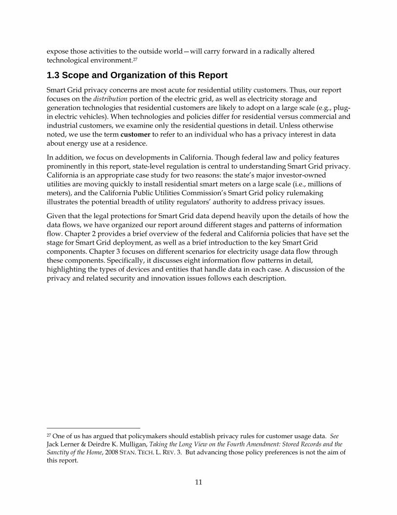
11

expose those activities to the outside world—will carry forward in a radically altered technological environment.27

1.3 Scope and Organization of this Report Smart Grid privacy concerns are most acute for residential utility customers. Thus, our report focuses on the distribution portion of the electric grid, as well as electricity storage and generation technologies that residential customers are likely to adopt on a large scale (e.g., plug-in electric vehicles). When technologies and policies differ for residential versus commercial and industrial customers, we examine only the residential questions in detail. Unless otherwise noted, we use the term customer to refer to an individual who has a privacy interest in data about energy use at a residence.

In addition, we focus on developments in California. Though federal law and policy features prominently in this report, state-level regulation is central to understanding Smart Grid privacy. California is an appropriate case study for two reasons: the state’s major investor-owned utilities are moving quickly to install residential smart meters on a large scale (i.e., millions of meters), and the California Public Utilities Commission’s Smart Grid policy rulemaking illustrates the potential breadth of utility regulators’ authority to address privacy issues.

Given that the legal protections for Smart Grid data depend heavily upon the details of how the data flows, we have organized our report around different stages and patterns of information flow. Chapter 2 provides a brief overview of the federal and California policies that have set the stage for Smart Grid deployment, as well as a brief introduction to the key Smart Grid components. Chapter 3 focuses on different scenarios for electricity usage data flow through these components. Specifically, it discusses eight information flow patterns in detail, highlighting the types of devices and entities that handle data in each case. A discussion of the privacy and related security and innovation issues follows each description.

27 One of us has argued that policymakers should establish privacy rules for customer usage data. See Jack Lerner & Deirdre K. Mulligan, Taking the Long View on the Fourth Amendment: Stored Records and the Sanctity of the Home, 2008 STAN. TECH. L. REV. 3. But advancing those policy preferences is not the aim of this report.

12

CHAPTER 2: Policy Frameworks: Smart Grid and Information Privacy 2.1 Federal Smart Grid Policy A national vision for the Smart Grid, articulated in the Energy Independence and Security Act of 2007 (EISA), highlights the potential for information about prices, supply and demand, and outages to help reduce peak demand, incorporate renewable energy sources and distributed generation, and speed recovery from interruptions.28 These changes in how the grid operates, in turn, have the potential to reduce the projected growth in energy demand, prices, and carbon emissions.29

The foundation of this plan is to integrate information technology into the electric grid. The National Institute of Standards and Technology (NIST) is coordinating an effort to foster interoperability, security, and privacy. EISA also directs the Federal Energy Regulatory Commission (FERC) to adopt Smart Grid standards and protocols through a rulemaking, once NIST’s efforts have “led to sufficient consensus.”30 According to its Smart Grid policy statement, FERC understands its mandate under EISA to include setting standards that “will be applicable” to “all elements of the grid, including communications with the ultimate consumer.”31 FERC, however, is unlikely to require states or utilities to adopt or use these standards.32 To lay the groundwork for this rulemaking, FERC released a Smart Grid Policy Statement, which sets forth FERC policy on cybersecurity, electric vehicles, and variable electricity generation as they relate to the bulk-power system. The Department of Energy (DOE) has an ongoing role in assessing Smart Grid deployments and technology under EISA.33

28 Pub. L. 110-140 §§ 1301, 1306.

29 See U.S. Department of Energy, What the Smart Grid Means to You and the People You Represent 2-3 (in Smart Grid Stakeholders Books series) (2009), http://www.oe.energy.gov/DocumentsandMedia/Regulators.pdf (stating that “[e]lectricity prices are forecast to increase 50% over the next 7 years”; “[n]ationwide, demand for electricity is expected to grow by 30% by 2030”; and “[i]f we do nothing, U.S. carbon emissions are expected to rise from 1700 million tons of carbon per year today to 2300 million tons of carbon by the year 2030”) (citations omitted).

30 EISA § 1305(d) (directing FERC to adopt standards and protocols to “insure smart-grid functionality and interoperability in interstate transmission of electric power, and regional and wholesale electricity markets”).

31 FERC, Smart Grid Policy, 74 Fed. Reg. 37,098-01 ¶ 22 (July 27, 2009).

32 See FERC, Smart Grid Policy, 74 Fed. Reg. 37,098-01 ¶ 23 (July 27, 2009) (“EISA, however, does not make any standards mandatory and does not give the Commission authority to make or enforce any such standards. Under current law, the Commission's authority, if any, to make smart grid standards mandatory must derive from the FPA.”).

33 EISA § 1302 (requiring DOE to report regularly to Congress on “the status of smart grid deployments nationwide and any regulatory or government barriers to continued deployment”).

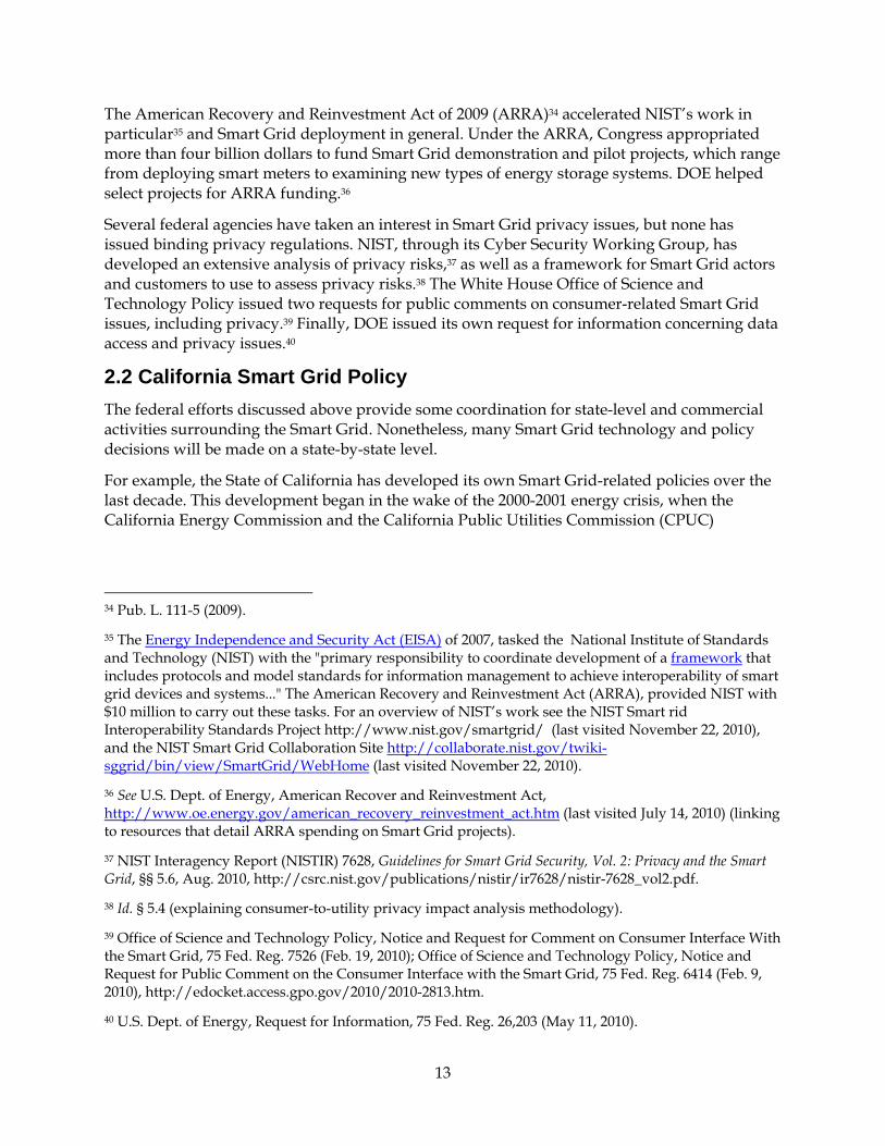
13

The American Recovery and Reinvestment Act of 2009 (ARRA)34 accelerated NIST’s work in particular35 and Smart Grid deployment in general. Under the ARRA, Congress appropriated more than four billion dollars to fund Smart Grid demonstration and pilot projects, which range from deploying smart meters to examining new types of energy storage systems. DOE helped select projects for ARRA funding.36

Several federal agencies have taken an interest in Smart Grid privacy issues, but none has issued binding privacy regulations. NIST, through its Cyber Security Working Group, has developed an extensive analysis of privacy risks,37 as well as a framework for Smart Grid actors and customers to use to assess privacy risks.38 The White House Office of Science and Technology Policy issued two requests for public comments on consumer-related Smart Grid issues, including privacy.39 Finally, DOE issued its own request for information concerning data access and privacy issues.40

2.2 California Smart Grid Policy The federal efforts discussed above provide some coordination for state-level and commercial activities surrounding the Smart Grid. Nonetheless, many Smart Grid technology and policy decisions will be made on a state-by-state level.

For example, the State of California has developed its own Smart Grid-related policies over the last decade. This development began in the wake of the 2000-2001 energy crisis, when the California Energy Commission and the California Public Utilities Commission (CPUC)

34 Pub. L. 111-5 (2009).

35 The Energy Independence and Security Act (EISA) of 2007, tasked the National Institute of Standards and Technology (NIST) with the "primary responsibility to coordinate development of a framework that includes protocols and model standards for information management to achieve interoperability of smart grid devices and systems..." The American Recovery and Reinvestment Act (ARRA), provided NIST with $10 million to carry out these tasks. For an overview of NIST’s work see the NIST Smart rid Interoperability Standards Project http://www.nist.gov/smartgrid/ (last visited November 22, 2010), and the NIST Smart Grid Collaboration Site http://collaborate.nist.gov/twiki-sggrid/bin/view/SmartGrid/WebHome (last visited November 22, 2010).

36 See U.S. Dept. of Energy, American Recover and Reinvestment Act, http://www.oe.energy.gov/american_recovery_reinvestment_act.htm (last visited July 14, 2010) (linking to resources that detail ARRA spending on Smart Grid projects).

37 NIST Interagency Report (NISTIR) 7628, Guidelines for Smart Grid Security, Vol. 2: Privacy and the Smart Grid, §§ 5.6, Aug. 2010, http://csrc.nist.gov/publications/nistir/ir7628/nistir-7628_vol2.pdf.

38 Id. § 5.4 (explaining consumer-to-utility privacy impact analysis methodology).

39 Office of Science and Technology Policy, Notice and Request for Comment on Consumer Interface With the Smart Grid, 75 Fed. Reg. 7526 (Feb. 19, 2010); Office of Science and Technology Policy, Notice and Request for Public Comment on the Consumer Interface with the Smart Grid, 75 Fed. Reg. 6414 (Feb. 9, 2010), http://edocket.access.gpo.gov/2010/2010-2813.htm.

40 U.S. Dept. of Energy, Request for Information, 75 Fed. Reg. 26,203 (May 11, 2010).

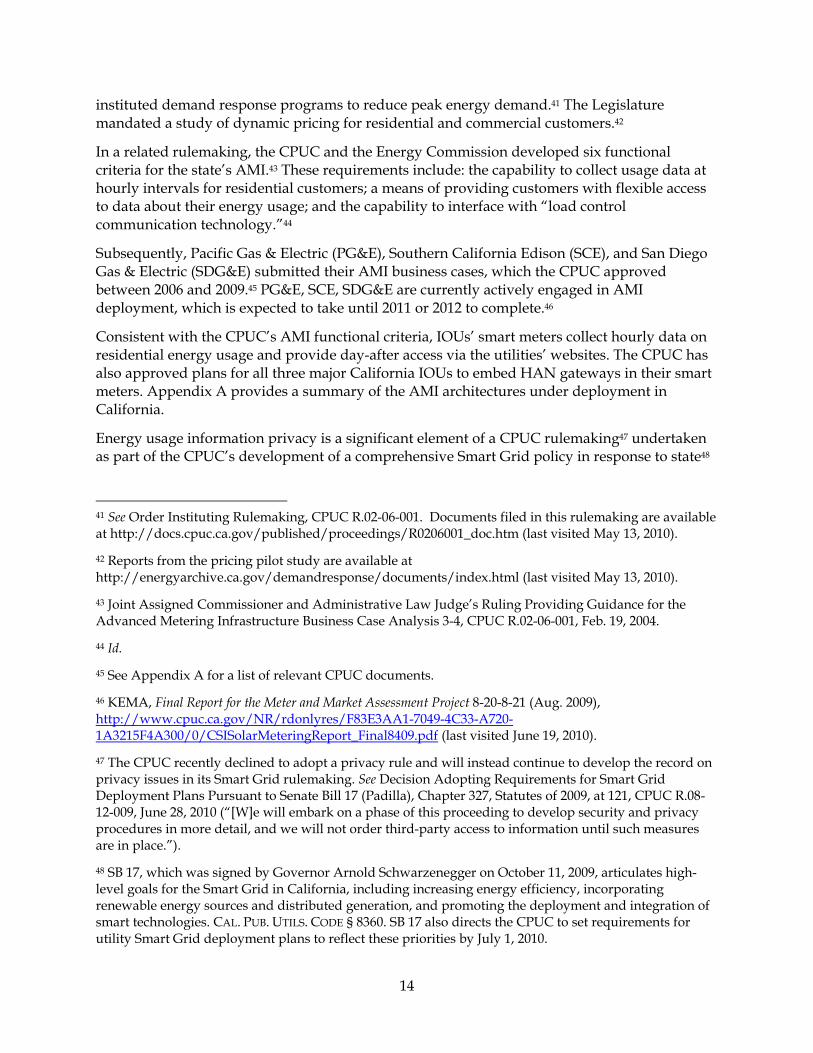
14

instituted demand response programs to reduce peak energy demand.41 The Legislature mandated a study of dynamic pricing for residential and commercial customers.42

In a related rulemaking, the CPUC and the Energy Commission developed six functional criteria for the state’s AMI.43 These requirements include: the capability to collect usage data at hourly intervals for residential customers; a means of providing customers with flexible access to data about their energy usage; and the capability to interface with “load control communication technology.”44

Subsequently, Pacific Gas & Electric (PG&E), Southern California Edison (SCE), and San Diego Gas & Electric (SDG&E) submitted their AMI business cases, which the CPUC approved between 2006 and 2009.45 PG&E, SCE, SDG&E are currently actively engaged in AMI deployment, which is expected to take until 2011 or 2012 to complete.46

Consistent with the CPUC’s AMI functional criteria, IOUs’ smart meters collect hourly data on residential energy usage and provide day-after access via the utilities’ websites. The CPUC has also approved plans for all three major California IOUs to embed HAN gateways in their smart meters. Appendix A provides a summary of the AMI architectures under deployment in California.

Energy usage information privacy is a significant element of a CPUC rulemaking47 undertaken as part of the CPUC’s development of a comprehensive Smart Grid policy in response to state48

41 See Order Instituting Rulemaking, CPUC R.02-06-001. Documents filed in this rulemaking are available at http://docs.cpuc.ca.gov/published/proceedings/R0206001_doc.htm (last visited May 13, 2010).

42 Reports from the pricing pilot study are available at http://energyarchive.ca.gov/demandresponse/documents/index.html (last visited May 13, 2010).

43 Joint Assigned Commissioner and Administrative Law Judge’s Ruling Providing Guidance for the Advanced Metering Infrastructure Business Case Analysis 3-4, CPUC R.02-06-001, Feb. 19, 2004.

44 Id.

45 See Appendix A for a list of relevant CPUC documents.

46 KEMA, Final Report for the Meter and Market Assessment Project 8-20-8-21 (Aug. 2009), http://www.cpuc.ca.gov/NR/rdonlyres/F83E3AA1-7049-4C33-A720-1A3215F4A300/0/CSISolarMeteringReport_Final8409.pdf (last visited June 19, 2010).

47 The CPUC recently declined to adopt a privacy rule and will instead continue to develop the record on privacy issues in its Smart Grid rulemaking. See Decision Adopting Requirements for Smart Grid Deployment Plans Pursuant to Senate Bill 17 (Padilla), Chapter 327, Statutes of 2009, at 121, CPUC R.08-12-009, June 28, 2010 (“[W]e will embark on a phase of this proceeding to develop security and privacy procedures in more detail, and we will not order third-party access to information until such measures are in place.”).

48 SB 17, which was signed by Governor Arnold Schwarzenegger on October 11, 2009, articulates high-level goals for the Smart Grid in California, including increasing energy efficiency, incorporating renewable energy sources and distributed generation, and promoting the deployment and integration of smart technologies. CAL. PUB. UTILS. CODE § 8360. SB 17 also directs the CPUC to set requirements for utility Smart Grid deployment plans to reflect these priorities by July 1, 2010.

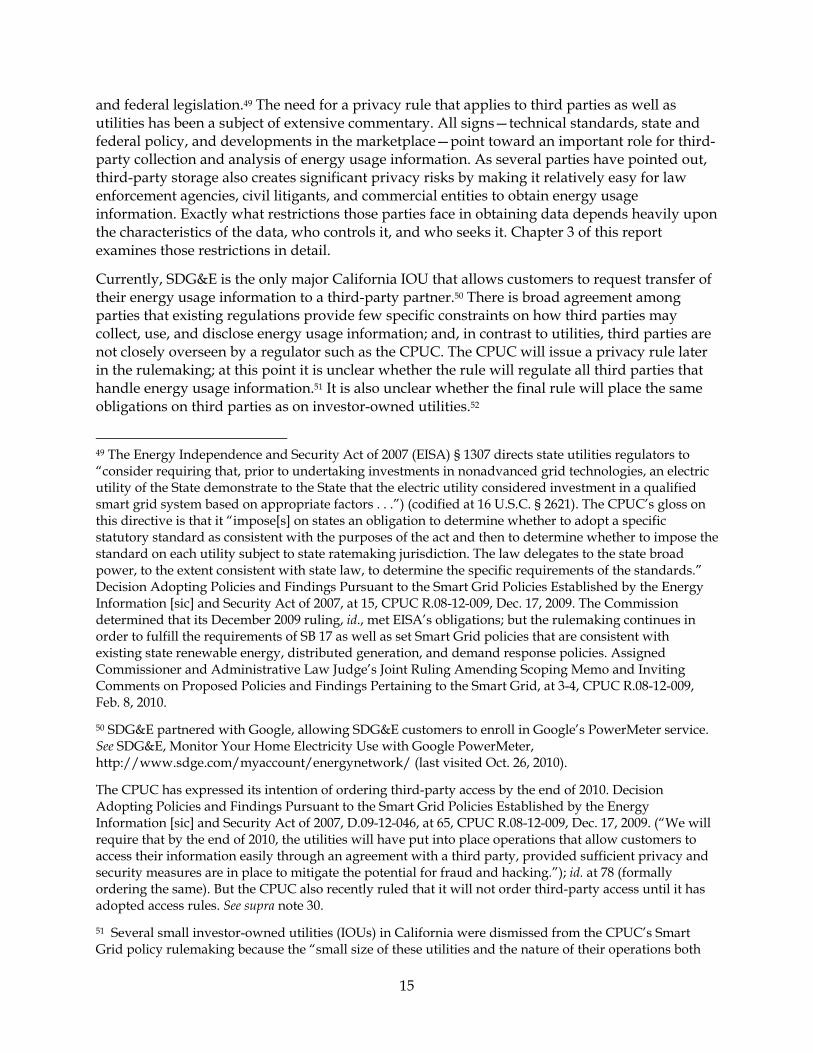
15

and federal legislation.49 The need for a privacy rule that applies to third parties as well as utilities has been a subject of extensive commentary. All signs—technical standards, state and federal policy, and developments in the marketplace—point toward an important role for third-party collection and analysis of energy usage information. As several parties have pointed out, third-party storage also creates significant privacy risks by making it relatively easy for law enforcement agencies, civil litigants, and commercial entities to obtain energy usage information. Exactly what restrictions those parties face in obtaining data depends heavily upon the characteristics of the data, who controls it, and who seeks it. Chapter 3 of this report examines those restrictions in detail.

Currently, SDG&E is the only major California IOU that allows customers to request transfer of their energy usage information to a third-party partner.50 There is broad agreement among parties that existing regulations provide few specific constraints on how third parties may collect, use, and disclose energy usage information; and, in contrast to utilities, third parties are not closely overseen by a regulator such as the CPUC. The CPUC will issue a privacy rule later in the rulemaking; at this point it is unclear whether the rule will regulate all third parties that handle energy usage information.51 It is also unclear whether the final rule will place the same obligations on third parties as on investor-owned utilities.52

49 The Energy Independence and Security Act of 2007 (EISA) § 1307 directs state utilities regulators to “consider requiring that, prior to undertaking investments in nonadvanced grid technologies, an electric utility of the State demonstrate to the State that the electric utility considered investment in a qualified smart grid system based on appropriate factors . . .”) (codified at 16 U.S.C. § 2621). The CPUC’s gloss on this directive is that it “impose[s] on states an obligation to determine whether to adopt a specific statutory standard as consistent with the purposes of the act and then to determine whether to impose the standard on each utility subject to state ratemaking jurisdiction. The law delegates to the state broad power, to the extent consistent with state law, to determine the specific requirements of the standards.” Decision Adopting Policies and Findings Pursuant to the Smart Grid Policies Established by the Energy Information [sic] and Security Act of 2007, at 15, CPUC R.08-12-009, Dec. 17, 2009. The Commission determined that its December 2009 ruling, id., met EISA’s obligations; but the rulemaking continues in order to fulfill the requirements of SB 17 as well as set Smart Grid policies that are consistent with existing state renewable energy, distributed generation, and demand response policies. Assigned Commissioner and Administrative Law Judge’s Joint Ruling Amending Scoping Memo and Inviting Comments on Proposed Policies and Findings Pertaining to the Smart Grid, at 3-4, CPUC R.08-12-009, Feb. 8, 2010.

50 SDG&E partnered with Google, allowing SDG&E customers to enroll in Google’s PowerMeter service. See SDG&E, Monitor Your Home Electricity Use with Google PowerMeter, http://www.sdge.com/myaccount/energynetwork/ (last visited Oct. 26, 2010).

The CPUC has expressed its intention of ordering third-party access by the end of 2010. Decision Adopting Policies and Findings Pursuant to the Smart Grid Policies Established by the Energy Information [sic] and Security Act of 2007, D.09-12-046, at 65, CPUC R.08-12-009, Dec. 17, 2009. (“We will require that by the end of 2010, the utilities will have put into place operations that allow customers to access their information easily through an agreement with a third party, provided sufficient privacy and security measures are in place to mitigate the potential for fraud and hacking.”); id. at 78 (formally ordering the same). But the CPUC also recently ruled that it will not order third-party access until it has adopted access rules. See supra note 30.

51 Several small investor-owned utilities (IOUs) in California were dismissed from the CPUC’s Smart Grid policy rulemaking because the “small size of these utilities and the nature of their operations both

16

2.3 Relating Smart Grid Architecture to Information Privacy Frameworks Before we delve into the details of Smart Grid information flows and their attending privacy risks, it is useful to consider key architectural choices that inform data flow in the Smart Grid and therefore substantively influence the possible privacy outcomes. As the discussion in Chapter 3 will make evident, privacy risks depend heavily upon the characteristics of a given data flow—the nature of the data, who receives data, and what a given entity plans to do with data.

Attending to privacy issues is considerably simpler if a semi-permeable boundary is drawn around customers’ homes, say at the electric meter, that lets information in but not out. This would be a high-level privacy aware design strategy. Conceptually speaking, utilities and device manufacturers could be made subject to a principle of minimizing HAN devices’ dependence on communicating with entities outside the home. A high-level architecture that might emerge from this approach is one in which utilities broadcast one-way price and event signals. Customers’ energy management systems would control HAN devices based on these signals and customers’ preferences, such as whether they will tolerate electricity interruptions for certain devices. The smart meter would serve only the basic function of reporting to the utility how much electricity a customer consumed, and when.

Though setting up a one-way gate for information around the home would mitigate many of the privacy risks we discuss in Chapter 3,53 this approach is also at odds with policies in California and elsewhere encouraging the development of two-way communications involving smart meters and HAN gateways. Moreover, Smart Grid policy in California, in other states, and at the national level envisions expansive roles for third parties. Absent a reversal of these policies, the complicated privacy and security risks involving information flows in and out of the home, increasing access by third parties, and remote management of in-home devices must be addressed with a more nuanced and integrated approach.

If, as current trends indicate, California and the nation choose to embed two-way communication within the Smart Grid, developing a conceptual map of important data flows and a privacy framework to guide technical and policy choices becomes ever more essential.

Appropriately, Smart Grid policy makers—the CPUC and NIST, in particular—and participants in the proceedings54 have embraced frameworks based on a set of “Fair Information Practice”

increase the costs and diminish the benefits of the EISA requirements.” Decisions Adopting Policies and Findings Pursuant to the Smart Grid Policies Established by the Energy Information and Security [sic] Act of 2007, at 2, CPUC R.08-12-009, Dec. 17, 2009. This left the three major IOUs—Pacific Gas & Electric, Southern California Edison, and San Diego Gas & Electric—as parties. Publicly owned utilities are not subject to CPUC jurisdiction.

52 See section 3.1.2.

53 Meter data collected at short time intervals would not be eliminated under this approach. This type of Smart Grid data carries its own privacy risks.

54 See Joint Comments of Center for Democracy & Technology and the Electronic Frontier Foundation on Proposed Findings and Policies Pertaining to the Smart Grid 14-26 (filed with CPUC, Mar. 9, 2010).

17

principles (FIPs) that establish ongoing rights and obligations to govern information about individuals held by smart grid players.55 FIPs conceptualize privacy as the right to informational self-determination that affords individuals control over personal information to protect individual autonomy, self-development, and intimacy.56 Statements of the FIPs vary, but a recent statement by the Department of Homeland Security provides widely accepted principles and definitions. 57 In DHS’s statement, FIPs comprise the following principles:

Transparency: organizations should provide notice to individuals regarding their use, disclosure, and retention of personally identifiable information (PII).

Individual participation: organizations should seek individual consent to collect, disclose, and retain PII.

Purpose specification: organizations should articulate specific purposes for collecting PII, and specific uses for PII they collect.

Data minimization: organizations should collect only PII that is “directly relevant and necessary to accomplish the specified purpose(s)” and retain data no longer than necessary.

Use limitation: organizations should use PII only for the purposes stated in their notices.

55 Another way to view Smart Grid privacy would be in terms of information ownership; that is, ask simply, “Who owns the data?” This property-based framework was popularized in Lawrence Lessig’s Code and Other Laws of Cyberspace (1999) (see in particular pp. 156-163) but has few followers among privacy law scholars and practitioners. See Marc Rotenberg, Fair Information Practices and the Architecture of Privacy (What Larry Doesn’t Get), 2001 STANFORD TECHNOLOGY LAW REVIEW 1, http://stlr.stanford.edu/STLR/Articles/01_STLR_1; Paul M. Schwartz, Beyond Lessig’s Code for Internet Privacy: Cyberspace Filters, Privacy-Control, and Fair Information Practices, 2000 WISCONSIN LAW

REVIEW 743. It is inaccurate to describe U.S. privacy statutes as taking a property-based approach. Numerous information privacy statutes—including the Video Privacy Protection Act, the Privacy Act, and the Cable Communications Act, among others—provide detailed rules to protect individuals’ expectations of privacy in transactions involving transfers of data for specifically stated purposes. See Schwartz, Beyond Lessig’s Code, at 779; Rotenberg, Fair Information Practices, ¶¶ 26-35.

Unfortunately, viewing personal information as property has gained a following among policymakers. See, e.g., Office of Science and Technology Policy, Notice and Request for Public Comment, 75 Fed. Reg. 7526, 7527 (seeking comment on the question, “Who owns the home energy usage data?”). See also Department of Energy, Request for Information: Implementing the National Broadband Plan by Empowering Consumers and he Smart Grid: Data Access, Third Party Use, and Privacy, 75 Fed. Reg. 26,203 (May 11, 2010) (seeking comment on “[w]ho owns energy consumption data”).

56 This conception of privacy goes back to some of the earliest legal scholarship on privacy law. See Samuel D. Warren & Louis D. Brandeis, The Right to Privacy, HARVARD LAW REVIEW, vol. 4, p. 193 (1891). For a recent review of the state of privacy law and scholarship, see Daniel J. Solove, A Taxonomy of Privacy, 154 UNIVERSITY OF PENNSYLVANIA LAW REVIEW 477 (2006).

57 Issued Dec. 28, 2008, at http://www.dhs.gov/xlibrary/assets/privacy/privacy_policyguide_2008-01.pdf.

18

Data quality and integrity: organizations should keep PII accurate, relevant, timely, and complete.

Security: organizations should implement adequate safeguards to protect against loss, unauthorized use, modification, and unintended disclosure.

Accountability and auditing: organizations should audit employees’ and contractors’ actual use of PII, to ensure compliance with the other FIPs.

While few U.S. information privacy statutes implement all of these principles, and U.S. privacy laws are typically limited to specific types of information (e.g., telecommunications records; healthcare information) and relationships (e.g., the customer-service provider relationship in the telecommunications sector; or patient-physician), FIPs are broadly accepted world-wide as the operational reference for privacy rights and obligations. For this reason, the constituent principles provide a useful guide throughout the remainder of this report.

19

CHAPTER 3: Privacy Risks in Smart Grid Information Flows Smart Grid data will not follow a single, well-defined pathway. Instead, the Smart Grid will support a variety of information flows. This chapter provides a detailed look at those information flows, both at the technical level (which devices are involved and which actors have access to information) and at the legal level (which statutes and regulations currently apply).

3.1 Meter Data and Energy Usage Information Privacy Risks 3.1.1 Meter Data Sent from Meter to Utility A fundamental data flow in the Smart Grid involves meter data going from the meter to the utility.58 The utility-provided meter measures electricity consumption over time and may store it before transmitting the data to the utility. Smart meters are capable of taking readings every few seconds, but in California at least, they do not send such fine-grained data to utilities. Instead, smart meters send hourly data to utilities, typically in several batches per day.59

58 The terms used in the report are drawn from several sources: SmartGrid/AEIC AMI Interoperability Standard Guidelines for ANSI C12.19 End Device Communications and Supporting Enterprise Devices, Networks and Related Accessories Version 2.0, Draft 8, Revision 3, at 11-20 (June 10, 2010), http://collaborate.nist.gov/twiki-sggrid/pub/SmartGrid/PAP05MeterProfiles/SmartGrid-AEIC-Standard-For-Interoperability-v2.0-DRAFT-8.3--06-10-10.doc; Smart Grid Interoperability Panel, PAP10: Standard Energy Usage Information, http://collaborate.nist.gov/twiki-sggrid/bin/view/SmartGrid/PAP10EnergyUsagetoEMS (last visited Aug. 26, 2010) (describing PAP10’s purpose as the development of “data standards to exchange fine grained and timely information about energy usage”); and California Energy Commission, Proposed Load Management Standards (Draft Committee Report), at 1-2, CEC-400-2008-027-CTD (Nov. 2008), http://www.energy.ca.gov/2008publications/CEC-400-2008-027/CEC-400-2008-027-CTD.PDF.

59 Based on informal discussions with CPUC staff and individuals knowledgeable about current smart meter technology, we understand that the smart meters deployed by California IOUs transmit customer usage data three times per day. This scheduling is necessary to avoid creating congestion in the utilities’ backhaul networks. Thus, while the utilities collect, and provide to customers or third parties, data at hourly increments, there may be a lag of several hours between measurement by the meter and transmission to the utility. Moreover, usage data generally is not available to customers until the next day. See supra notes 34 and 36.

This report adopts terms that reflect the separation of the meter and the HAN gateway, as well as the distinction between data about energy consumption and information that can be used to manage or control devices.

Meter data: any data collected by a utility-owned electric meter. 1

Energy usage information: consumption and time-of-use, which can be measured by a range of devices, including customer-owned metering devices that send data directly to third parties.1

Load control information: information that helps achieve demand response, particularly through automated means.1 Prices and device control signals are examples Load management information

20

Utilities use meter data for a variety of purposes. They use fine-grained meter data to apply time-variant pricing, including time-of-use rates, critical peak pricing, and real-time pricing.60 Utilities may also use meter data for load research, e.g., to better understand which devices customers are using at a given time.61 Data mining algorithms may help utilities sell targeted advertising to customers.62 A utility might detect meter tampering by comparing current data with historical records.63 Utilities also make the data available to customers through their websites to improve customers’ understanding of their energy usage and promote load shifting to reduce peak demand.64

This information flow raises several privacy issues. The discussion below illustrates how legal protections vary depending on where and how the data is accessed.

Figure 2: Meter data flow between smart meter and utility

A smart meter (in magenta, attached to the side of the house) collects, stores, and transmits short-interval meter data from the home to the utility (drawn in blue). Smart meters also facilitate two-way communications between the meter and the utility. Energy usage information is depicted as a bidirectional arrow composed of discrete square elements. Graphics Credit: Brian P. Miller Photo & Design, http://www.brianpmillerphotography/

60 CAL. PUB. UTILS. CODE § 502(c) (“The commission may, at any time, authorize an electrical corporation to offer residential customers the option of receiving service pursuant to time-variant pricing and to participate in other demand response programs.”); CAL. PUB. UTILS. CODE § 502(a)(2) (“‘Time-variant pricing’ includes time-of-use rates, critical peak pricing, and real-time pricing, but does not include programs that provide customers with discounts from standard tariff rates as an incentive to reduce consumption at certain times, including peak time rebates.”); CAL. PUB. UTILS. CODE § 745 (forbidding utilities from “employ[ing] mandatory or default time-variant pricing” before January 1, 2013).

61 SCE, SmartConnect Use Case: C8 – Load Researchers Perform Analyses Using SmartConnect Data, http://www.sce.com/NR/rdonlyres/D7F9B623-2DA0-4E31-A98C-5537748279BB/0/C8_Use_Case_090120.pdf (last visited June 19, 2010).

62 SCE, SmartConnect Use Case: C7 – Utility Uses SmartConnect Data for Targeted Marketing Campaigns, http://www.sce.com/NR/rdonlyres/E2927535-15B3-41F3-AE88-B06CE760225F/0/C7_Use_Case_081229.pdf (last visited June 19, 2010).

63 SCE, SmartConnect Use Case: B3 - Utility detects tampering or theft at customer site, http://www.sce.com/NR/rdonlyres/943C8D62-0011-4959-9C5A-620684B34CF3/0/ARCHB3USECASEv12050106.pdf (last visited June 19, 2010).

64 See Cal. Pub. Utils. Code § 8360(d) (specifying demand response as a grid modernization policy goal); id. § 8366(d) (same).

21

3.1.1.1 Data stored in meter

Smart meters store meter data internally. Under current AMI architectures, utilities control the meters; they do not grant access to other parties without customer’s consent. But suppose that some individual—a hacker or a burglar, for example—wants to obtain data about a specific customer and takes advantage of the smart meter’s network connection to remotely hack into the meter. Unlike a mechanical meter, which requires proximity to access and provides no historical data about energy usage, smart meters can be broken into remotely and contain an uncertain amount of data about occupant behavior. This information could facilitate threats to a customer’s physical security by providing detailed information about when he or she is at home.

Since smart meters apply access controls to stored data (and hence provide a technology-based means for authorizing access to data), this conduct is prohibited under state and federal “anti-hacking” laws. Specifically, the federal Computer Fraud and Abuse Act (CFAA) prohibits accessing a “protected computer” without authorization or in excess of authorization. To the extent that smart meters and other smart grid components are “computers” within the meaning of the CFAA,65 the statute prohibits others from breaking into them and thereby obtaining information. At the state level, California prohibits obtaining data by knowingly gaining unauthorized access to a computer,66 such as a smart meter. A qualification to applying these laws to smart meter intrusions is that an intrusion must cause “loss” to constitute an offense. Loss is defined broadly under the CFAA to include “any reasonable cost to any victim,” including the costs of responding to an intrusion, restoring lost data, and lost revenue resulting from an incident.67

Two characteristics of computer abuse statutes distinguish them from many of the other laws and regulations discussed in this report. First, they apply to “information” and “data.” These broad terms presuppose nothing about the value of the data to the customer, the utility, or any other party. Nor do they require that the information be “personally identifiable” or “private.”

Second, neither federal nor state computer abuse laws require the owner of a computer system to provide any particular level of technical protection for data in order to qualify for relief. In principle, data stored on a smart meter, and protected only by a widely known, globally used password could still be protected from unauthorized access under federal and state laws. Note that, although the utility owns the meter, the CFAA permits “[a]ny person who suffers damage or loss by reason of a violation” of the Act to sue for damages.”68 Thus, if a customer suffers sufficient loss as a result of a hacked meter, he or she may file a civil suit against the

65 A computer is “protected” by the CFAA if it is used in or affects interstate or foreign commerce. 18 U.S.C. § 1030(e). This definition is jurisdictional; “protected” here simply means that a computer is covered by the CFAA, not that it is protected against unauthorized access in any technical, or even contractual, sense.

66 Cal. Penal Code § 502. All 50 states have similar laws. See Susan W. Brenner, State Cybercrime Legislation in the United States of America: A Survey, 7 RICH. J.L. & TECH. 28, ¶ 15 n.37 (2001), at www.richmond.edu/jolt/v7i3/article2.html (listing the laws).

67 18 U.S.C. § 1030(e)(11).

68 18 U.S.C. § 1030(g); see also Expert Janitorial, LLC v. Williams, 2010 WL 908740 (E.D. Tenn., Mar. 12, 2010).

22

perpetrator.69 In addition, the utility may sue civilly if it suffers loss (e.g., by conducting a forensic investigation of the incident, sending a technician to replace the meter, etc.). Finally, the government may file criminal charges against the party (or parties) who gain unauthorized access to a smart meter.

3.1.1.2 Data in transit.

As data moves from the smart meter to the utility—typically via a radio frequency network that the utility operates solely for its own use—a separate set of statutes protects data confidentiality. The federal Wiretap Act prohibits a person who is not a party to a communication from intentionally “intercepting” the communication.70 The California Penal Code contains a similar prohibition.71 As with computer fraud laws, anti-wiretapping laws do not require the parties to the communication—the utility and the customer in this case—to take technical precautions (e.g., encrypting the contents of the communication) against interception. There is an exemption to the Wiretap Act for “an electronic communication made through an electronic communication system that is configured so that such electronic communication is readily accessible to the general public.”72 If utilities used radio-frequency broadcasts to transmit price information, for example, those communications would probably be exempt from the Wiretap Act. Communications between a smart meter and a utility over a cellular or spread-spectrum network, however, involve well-defined senders and recipients and, at a technical level are not “readily accessible to the general public.” As a result, they would be protected by the Wiretap Act.

3.1.1.3 Data retained by utility.

Once meter data reaches the utility, a customer’s privacy interests are legally protected in two distinct ways. First, like data stored on a smart meter, meter data stored on a utility’s computers is protected by federal and state anti-hacking laws.

Second, once a utility acquires data from a customer’s smart meter, it has certain affirmative obligations to keep the data confidential. The remainder of this section describes (1) utilities’ obligations to protect customer usage data from unauthorized disclosures and (2) the circumstances under which law enforcement agencies and parties in civil litigation may compel utilities to produce meter data.

69 “Loss” under the CFAA is expansive. It means “any reasonable cost to any victim, including the cost of responding to an offense, conducting a damage assessment, and restoring the data, program, system, or information to its condition prior to the offense, and any revenue lost, cost incurred, or other consequential damages incurred because of interruption of service.” 18 U.S.C. § 1030(e)(11).

70 18 U.S.C. § 2511. “Interception” includes the activity of acquiring the contents of a communication in real time. This is the circumstance most directly related to the information flow described in the main text. But “interception” describes a broader range of conduct involving the acquisition of a communication’s contents by a person who did not send a message and is not one of its intended recipients; “interception” is not limited to acquisition that is contemporaneous with transmission. The exact boundaries of “interception,” however, remain unclear.

71 CAL. PENAL CODE §§ 630-632.7.

72 18 U.S.C. § 2511(2)(g)(i).

23

These different stages of data flow from the smart meter to the utility raise an array of privacy issues, which we explore in the remainder of this section. Utilities in California are not subject to a specific, statutory requirement to keep information about customers confidential. This is in contrast to other entities that provide some of the same services as electric utilities. For example, electric service providers are required by statute to keep “customer information” confidential, unless the customer authorizes the release of information.73 Similarly, telephone companies and Internet service providers are subject to a variety of federal and state restrictions on disclosing data to private parties and law enforcement agencies and other governmental entities.

California lacks analogous statutory rules for IOUs. IOUs operate under tariffs—“official rates and terms of service”74—that require them to keep customer information confidential. For example, PG&E promises not to “release confidential information, including financial information, to a third party without the customer’s electronic signature or the [sic] written consent.”75 A CPUC rule requires investor owned utilities to obtain consent before sharing “customer information” with an “affiliate.”76 The CPUC has the authority to punish violations of utilities’ own privacy rules77 as well enforce its affiliate transaction rules.78

3.1.1.4 Protection Against Unauthorized Disclosures: Security Breach Notification Laws

IOUs—like other entities that do business in California and are thus subject to its security breach notification (SBN) law—must notify customers if “unencrypted personal information” about them “was, or is reasonably believed to have been, acquired by an unauthorized person.”79 SBN laws, however, have significant limitations where customer usage data from the

73 CAL. PUB. UTILS. CODE § 394.4.

74 CPUC, Utility Tariff Information, http://www.cpuc.ca.gov/PUC/energy/Electric+Rates/utiltariffs/ (last visited June 24, 2010).

75 PG&E, Electric Rule 9 § M, (effective date Jan. 20, 2009), http:// www.pge.com/tariffs/tm2/pdf/ELEC_RULES_9.pdf. See also PG&E, Opening Comments on Proposed Policies and Findings Pertaining to the Smart Grid, at 14 (Mar. 9 2010) (citing this tariff to support its argument that the Commission’s existing customer privacy rules should be the basis of rules regarding third-party access to customer energy usage data and other customer-specific data”).

76 “Customer information” means “non-public information and data specific to a utility customer which the utility acquired or developed in the course of its provision of utility services.” CPUC D. 97-12-088, revised by D.98-08-035 and amended by D.98-12-075. “‘Affiliate’ means any person, corporation, utility, partnership, or other entity 5 per cent or more of whose outstanding securities are owned, controlled, or held with power to vote, directly or indirectly either by a utility or any of its subsidiaries, or by that utility’s controlling corporation and/or any of its subsidiaries.” Id.

77 The most obvious enforcement route would use the Commission’s power to punish contempt: “Every public utility, corporation, or person which fails to comply with any part of any order, decision, rule, regulation, direction, demand, or requirement of the commission or any commissioner is in contempt of the commission, and is punishable by the commission for contempt in the same manner and to the same extent as contempt is punished by courts of record.” CAL. PUB. UTILS. CODE § 2113.

78 Violations of utility privacy rules might also be subject to punishment by the Federal Trade Commission, as discussed later in this report. See infra Part 3.d.i.

79 CAL. CIV. CODE § 1798.82. Forty-six states and the District of Columbia have similar laws. Perkins Coie, Security Breach Notification Chart, http://www.perkinscoie.com/statebreachchart/chart.pdf (last visited June 22, 2010). Congress has considered, but has not passed, numerous bills that would create a

24

Smart Grid is concerned. A duty to notify applies only to breaches involving “personal information,” which California’s SBN law defines to mean an individual’s name in combination with certain categories of information, such as an account number80 Hour-by-hour traces of energy consumption are not among the categories of personal information listed in California’s SBN. Unless an account number or other types of statutorily protected personal information accompany a breach of this information , it would not trigger a duty to notify affected customers.

3.1.1.5 Protection Against Compelled Disclosures

Like the unauthorized acquisitions of private information discussed above, certain types of lawful acquisitions can harm individual privacy. We discuss two scenarios of this type: law enforcement access and civil litigant access. Both involve a third party—a law enforcement agent or a civil litigant—compelling the production of private data from a utility. Though we presume the transfers that we discuss to be lawful, they nonetheless intrude upon individual privacy because they interfere with a person’s ability to control information about him or her.

Law Enforcement Agencies.

CPUC rules do not regulate law enforcement access to data. The burden that a law enforcement agency must meet in order to obtain customer-specific data is unclear. One possibility is that customers have a reasonable expectation of privacy in the detailed record of in-home activities that meter data reveals, implying that law enforcement agents must obtain a warrant in order to gain access to the data.81 One reading of the U.S. Supreme Court’s ruling in Kyllo v. United States,82 which involved infrared camera surveillance of individuals inside their own home, supports this view.83 The CPUC has also interpreted California Supreme Court case law on the state constitutional right to privacy84 to mean that law enforcement agents must obtain a search warrant or judicially issued subpoena before demanding utility customer records.85

federal security breach notification requirement. An “unauthorized person” may have obtained access either through accident (e.g., a misconfigured website) or a malicious attack. California’s SBN law requires notification under both circumstances.

80 CAL. CIV. CODE § 1798.82(e).

81 For an argument in favor of this view, see Joint Comments of Center for Democracy & Technology and the Electronic Frontier Foundation on Proposed Findings and Policies Pertaining to the Smart Grid 10-12 (filed with CPUC, Mar. 9, 2010).

82 533 U.S. 27 (2001).

83 See Jack I. Lerner & Deirdre K. Mulligan, Taking the ‘Long View’ on the Fourth Amendment: Stored Records and the Sanctity of the Home, 2008 STAN. TECH. L. REV. 3.

84 CAL. CONST., art. I, §§ 1, 13.

85 CPUC, Opinion Denying Petition of California Narcotic Officers’ Association to Modify Decision 90-12-121, D.01-07-032, Jul. 12, 2001; see also Joint Comments of the Center for Democracy and Technology and the Electronic Frontier Foundation on Proposed Policies and Findings Pertaining to the Smart Grid, at 31-33, R.08-12-009, Mar. 9, 2010 (discussing CPUC Decision 01-07-032 and the underlying line of cases) [“CDT/EFF Opening Comments”].

25

As the CyberKnowledge/Berkeley Report points out, however, a second possibility is that law enforcement agents may simply request a customer’s meter data.86 The California Court of Appeals has held that utility records are business records that are voluntarily handed over to a third party, and thus devoid of a reasonable expectation of privacy.87 Federal courts have reached the same conclusion.88

Between these two extremes is a third possibility: that law enforcement agents must present a grand jury subpoena, which is quicker than a judge-issued subpoena and does not involve the oversight of a neutral decision-maker.89 This appears to be the common practice among law enforcement officials in California.90

Given the increased details that smart meter data may reveal, it remains to be seen whether the CPUC, California courts, or the California legislature will close these gaps and clarify the law. It is clear, however, that any of these branches of government have significant latitude to set rules regulating law enforcement agencies’ access to meter data.

Civil Litigants. Meter data is available to litigants in a civil case on relatively easy terms. A party in a civil suit—such as a divorce, where meter data could be highly relevant—may obtain the data from an IOU with a subpoena.91 Neither the utility nor the party issuing the subpoena needs to notify the individual(s) whose activities are reflected in this data. This significantly limits the opportunity of the customer to assert a privacy interest and object to the subpoena.

Again, the contrast to other domains involving detailed data about individual activities is striking. For example, in California, in the financial, insurance, and health care domains, individuals must be given an opportunity to object to subpoenas demanding their personal information.92 Subpoenas for telephone records contain an extra procedural safeguard: they must be signed “by the consumer whose records are requested” in order to be valid.93

3.1.2 Energy Usage Information Collected by a Customer-Owned Metering Device A significant shift in the Smart Grid, relative to its predecessor, is that it will enable entities other than utilities—third parties—to collect meter data. Smart grid data can be obtained either 86 CyberKnowledge/Berkeley Report, supra note 3, at 25 (discussing Cal. Penal Code § 1326.1(e), which states that “[n]othing in this section shall preclude the holder of the utility records from voluntarily disclosing information or providing records to law enforcement upon request”).

87 People v. Stanley, 72 Cal. App. 4th 1547, 1552-54 (2d App. Dist. 1999); CyberKnowledge/Berkeley Report, supra note 3, at 26-27.

88 See United States v. Starkweather, 1992 U.S. App. LEXIS 20207 (9th Cir.); CyberKnowledge/Berkeley Report, supra note 3, at 26 (discussing cases).

89 See CyberKnowledge/Berkeley Report, supra note 3, at 30-31 (noting that an investigator may obtain a grand jury subpoena “can be done in as little as ten minutes”).

90 See CyberKnowledge/Berkeley Report, supra note 3, at 30-31 (reporting, based on interviews with current and former U.S. Attorneys, that investigators typically use grand jury subpoenas in non-emergency situations, in part because utilities typically decline to produce customer records voluntarily).

91 CAL. CODE CIV. PROC. §§ 2010.410-2020.440.

92 CAL. CODE CIV. PROC. § 1985.3(a), (c).

93 CAL. CODE CIV. PROC. § 1985.3(f).

26

from the utilities or directly from the individual’s network or devices. This section considers the privacy issues arising when data is obtained directly from individuals.

Individuals may purchase94 their own metering devices and use them to send data entirely separately from utility-owned infrastructure. Figure 3. Currently, these devices cost from $20 to $200.95 Alternatively, individuals may choose to use devices, such as The Energy Detective (TED). TED uses current transformers (CTs) to measure electricity consumption; basically, two clips placed around the electrical wires entering a home’s circuit breaker measure how much electricity flows into the house. The device uses this connection to measure electricity consumption at one-second intervals when the CTs are attached to breaker panels. 96 TED devices can also connect to the Internet and send energy usage information to third parties who may, in turn, present analyzed data via cell phone or Web-based applications.97

The devices that customers buy on their own may measure electricity usage at both device and household levels. (Figure 3 shows device-level measurements.) For instance, customers may have end-use metering to support distributed generation, or monitor discreet loads. 98

94 Presumably customers will also be able to lease, rent, or use a third-party-provided metering device. We use the term “customer-owned metering device” to describe all of these cases, the common thread being that the metering device is not the utility meter.

95 ChooseRenewables, Energy Usage Monitors, https://www.chooserenewables.com/xcart/home.php?cat=266&gclid=CLXXlOyHo6ECFQ8bawodWBiSww (last visited June 20, 2010) (showing a list of energy usage monitors that customers can purchase).

96 TED, How Do I Install TED?, http://www.theenergydetective.com/about-ted/how-do-i-install-ted (last visited June 20, 2010); TED, Measuring Transmitting Unit (MTU) and Current Transformers (CTs), http://www.theenergydetective.com/which-ted.html.

97 TED, Third Party Applications for TED 5000, http://www.theenergydetective.com/ted-5000/3rd-party-apps (last visited June 20, 2010).

98 ZigBee Alliance and HomePlug Powerline Alliance, Smart Energy Profile 2.0 Technical Requirement Document v0.5 at 57 (“end-use metering that includes additional meters installed in the premises to support distributed generation production or measurement of discreet loads.”) [“SEP 2.0 Technical Requirement Document v0.5”]

27

Figure 3: Meter data collected by customer-owned meter

A customer-owned metering device (at the top of the house) measures electricity consumption and other data, and sends the data over a general-purpose network (e.g., the Internet or a cellular network) to a third party (drawn in green in the upper left-hand corner of the figure) for collection and analysis. The third party might provide services such as presenting analyzed data or sending energy usage alerts to the customer. The utility-owned meter sends similar data to the utility over its own network, though the measurement interval and uses of data may be different. Graphics Credit: Brian P. Miller Photo & Design, http://www.brianpmillerphotography.com/

The differences in the device-specificity of usage information, the frequency with which energy usage data is measured and transmitted, and the potentially wide variety of third-party data recipients create a complex set of privacy issues. Data from the customer-owned metering device might not be transferred to or from the utility (though the utility will obtain data from its own meter); this could leave data from the customer’s metering device beyond the scope of CPUC regulations. The CPUC has considered privacy rules to govern third-party access to customer usage data, but it has not adopted a final rule.99

99 As the CPUC explains, “privacy protections and the reach of Commission jurisdiction are under review by legislation pending before the State Legislature. Legislative action may provide greater legal clarity in

28

Even if the CPUC (and utilities commissions in other states) do not regulate third parties, the data they handle will be subject to more general legal protections. For example, the general—but limited—protections offered by the federal Electronic Communications Privacy Act (ECPA), the Federal Trade Commission (FTC) Act, and state security breach notification laws still apply.100 As discussed in the next section, ECPA imposes few limits on how authorized recipients of meter data may use it, and it is questionable whether its protections against disclosure to law enforcement agencies apply to utilities and third parties that might handle this data. The FTC Act applies to a broad range of “unfair” or “deceptive” conduct that gives rise to privacy harm, but enforcement has been rare in cases in which a firm gives adequate notice of its data processing practices. Finally, security breach notification laws require firms to give notice after discovering unauthorized access to certain categories of personally identifiable information. As discussed above, however, as breach notification laws may not apply to many breaches.

Overall, customer-owned metering devices are not subject to the same level of public or regulatory review as utility-owned devices prior to going on the market. Moreover, the laws that do apply to third parties omit many FIPs, by failing to require third parties to specify the purposes for data collection, minimize data collection to what is necessary to achieve these purposes, and limit actual uses to the stated purposes. It remains to be seen whether utilities regulators, state legislatures, or other authorities will develop rules that are tailored for customer usage data.

3.1.3 Third Party Access to Energy Usage Information Held by Utilities This section discusses the acquisition of energy usage information from utilities by third parties, as shown in Figure 4. This section also highlights that the applicable privacy laws, and privacy regulators, change dramatically as information travels from the customer, to the utility, to one or more third parties.

3.1.3.1 Third party Access Via a Utility

Enabling this kind of information flow is a major priority of Smart Grid policy. Though San Diego Gas and Electric (SDG&E) and Sacramento Municipal Utility District (SMUD) are the only California utilities with programs in place to provide data to third parties, the CPUC is requiring all major IOUs to provide consumers and third parties approved by consumers with

this matter. If there is no action on this matter by the Legislature, then the Commission will consider inviting legal briefs to clarify the extent of the Commission’s jurisdiction and to recommend the best procedure for protecting consumer interests.” Decision Adopting Requirements for Smart Grid Deployment Plans Pursuant to Senate Bill 17 (Padilla), Chapter 327, Statutes of 2009, at 43 n.90, CPUC R.08-12-009, June 28, 2010.

100 See the discussion in Part 3.2.3 below.

29

usage data by the end of 2010.101 The CPUC proposed rules to govern third-party access to energy usage information, but as of this writing it has not adopted final rules.102

Two prominent third-party energy usage information-processing services—Google PowerMeter and Microsoft Hohm—are similar in overall design, though they have some underlying technical differences. Most importantly, both services obtain energy usage information directly from utilities, but only when customers choose to use the service. Utilities do not provide the information to Google or Microsoft without the customer’s consent.

To enroll in Google PowerMeter, users first authenticate themselves on the utility website, and then use the utility website to authorize Google PowerMeter to access their energy usage information.103 Google assigns each PowerMeter user a unique PowerMeter ID.104 The utility provides energy usage information to PowerMeter at 15-minute to hourly intervals, depending on the utility.105 The information is transferred to Google via an encrypted connection in a data format specified by Google.106 The information transfer is associated with the PowerMeter ID; customers do not need to provide Google Account username to the utility for the data transfer, nor do customers provide their utility account number to Google.107 Once the energy usage information is stored with PowerMeter, users can log in with Google Account username to view

101 CPUC Decision 09-12-046 (Dec. 17, 2009) at 3 (“Concerning electricity usage data, we require that SCE, PG&E and SDG&E provide consumers and third parties approved by consumers with usage data that is collected by the utility by the end of 2010.”).

102 Assigned Commissioner and Administrative Law Judge’s Joint Ruling Amending Scoping Memo and Inviting Comments on Proposed Policies and Findings Pertaining to the Smart Grid, Attachment B, CPUC R.08-12-009, Feb. 8, 2010, http://docs.cpuc.ca.gov/efile/RULINGS/113482.pdf.

103 Google PowerMeter, Enrollment, http://sites.google.com/site/powermeterpartners/enrollment (last visited June 20, 2010).

104 Google, Google PowerMeter API Data Model, http://code.google.com/apis/powermeter/docs/meter_api_datamodel.html (last visited June 20, 2010) (“The Google PowerMeter ID is a unique, 20-digit ID representing a user. The ID is issued when the user consents (on the Google PowerMeter web site) to Google PowerMeter program terms. To protect user privacy, the generated ID is specific to Google PowerMeter and cannot be linked to other Google service IDs for the same Google account. For more information, refer to the description of the device activation process.”)

105 Google, Google PowerMeter Privacy Policy Notice, http://www.google.com/powermeter/privacy (last visited June 20, 2010) (“The frequency of these readings depends on your utility; for example, some utilities will send hourly readings, others will send fifteen (15) minute interval readings throughout the day.”). Since utilities in California collect hourly data from residential customers, they cannot provide more fine-grained data.

106 Google, Google PowerMeter API Data Model, http://code.google.com/apis/powermeter/docs/meter_api_datamodel.html (last visited June 20, 2010).

107 Google, Google PowerMeter Privacy Policy Notice, http://www.google.com/powermeter/privacy (last visited June 20, 2010) (“Google creates a unique PowerMeter user identifier at the time of enrollment in your utility’s PowerMeter program. All data sent by your utility to Google will be tagged with this unique identifier only.”)

30

their information. Users can also choose to share their information with other PowerMeter users, on an opt-in basis.108

Microsoft Hohm adopts a different authentication process.109 A utility partnered with Hohm first provides three authentication questions to Hohm. After a utility customer answers these questions on Hohm website, Hohm provides the answers to the utility to authenticate the customer. If the authentication is approved by the utility, Hohm generates a customer ID and provides it to the utility. The utility then provides the customer’s energy usage information associated with the customer ID to Hohm in the XML format defined by Microsoft.

To address the problem that different third parties have their own formats for customer data, major California IOUs, Microsoft, Google, and others have proposed Open Automated Data Exchange (OpenADE) to standardize energy usage information exchange between utilities and third parties.110 NIST is also coordinating a working group to develop standards for the exchange of energy usage information.111

Figure 4: Energy usage information flow patterns involving third parties

108 Danan Sudindranath, Share your Power(Meter)!, http://blog.google.org/2010/03/share-your-powermeter.html (last visited June 20, 2010).

109 Microsoft, Integrating with Hohm – Registering Customers, http://msdn.microsoft.com/en-us/library/ee724246(v=MSDN.10).aspx (last visited June 20, 2010).

110 UCAIug OpenSG OpenADE Task Force, OpenADE 1.0 System Requirements Specification, http://www.smartgridipedia.org/images/0/0e/OpenSG_OpenADE_1.0_SRS.pdf (last visited June 20, 2010); OpenADE Charter, http://www.smartgridipedia.org/index.php/OpenADE_Charter (last visited July 17, 2010) (stating that price information will be included in OpenADE 2.0).

111 NIST, NIST Framework and Roadmap for Smart Grid Interoperability Standards, Release 1.0 79, NIST Special Publication 1108, http://www.nist.gov/public_affairs/releases/upload/smartgrid_interoperability_final.pdf (“Subsequent work in the first half of 2010 will drive a standardized information model for broader exchange of usage information.”).

31

Third parties may obtain energy usage information in several ways: from a utility, from another third party, or directly from a customer-owned meter. Graphics Credit: Brian P. Miller Photo & Design, http://www.brianpmillerphotography.com/ Some of the privacy risks associated with energy usage information transfers from utilities to third parties are now familiar: The information may be disclosed law enforcement agencies or civil litigants, as discussed in section 3.2.1. In addition, third parties’ business reasons for collecting the information may differ from those of utilities. Non-utility third parties may have economic incentives to use or share customer’s energy usage information, for example, as part of marketing campaigns.112 Third parties may also say little about what information they collect and use, and their disclosures may be in the form of lengthy, impenetrable privacy policies. All of these factors may make it difficult for customers to understand the effects of agreeing to information disclosures.

As discussed below, consumer protection agencies such as the Federal Trade Commission have imposed few substantive requirements on privacy policy disclosures, though recent enforcement actions may signal a change in approach.113 Furthermore, customers who seek to understand the information privacy practices of several competing third-party service providers will need to review each company’s privacy policy. Given how these documents are

112 See CDT/EFF Joint Opening Comments, supra note 54, at 26 (“Some third parties seeking access to customer data are likely to have business models based upon offering the consumer a service, perhaps for free, and then commercializing and selling the data.”).

113 See Wendy Davis, Sears Required To Destroy Tracking Data, Online Media Daily, Sept. 9, 2009 (quoting sources who opined that the Sears settlement marked a new disclosure standard at the FTC).

32

typically written, this would likely involve a significant investment of time and effort.114 Still, provided that privacy policies are publicly available, some individuals or entities (e.g., nonprofits) may be willing to analyze and compare them.115

Public Utilities Commission Regulation of Third Parties. Third parties that obtain customers’ energy usage information from utilities may be subject to two very different privacy regimes. First, by virtue of their dealing with utilities, they may be subject to indirect CPUC regulation. That is, the CPUC could require investor owned utilities to impose certain conditions on their third-party partners. In addition, the CPUC may adopt an access rule that directly regulates third party use, retention, and protection of customers’ energy usage information.116 As stated above, however, the CPUC has not adopted a final rule on this topic.

Applying General Data Privacy Laws to Third Parties. Irrespective of whether utilities regulators adopt privacy rules for third parties, they are subject to general state and federal data privacy and security laws. As discussed in section 3.2.1, these include:

Criminal prohibitions on obtaining data by intercepting it or hacking into the third party’s computers;

Security breach notification laws, which require a third party to notify customers in the event of unauthorized access to personally identifiable information.

Subpoena requirements for law enforcement agency and civil litigant access to data.

These restrictions are obviously limited in scope. Tariff rules provide some privacy protection by stating that the utility will not release “confidential information” to a third party—which, stated without qualification, includes private parties and governmental entities—without customer consent.117 Amending tariffs to reduce these protections, however, is far easier than

114 There are, of course, exceptions. See, e.g., Google, Google PowerMeter Privacy Policy Notice, http://www.google.com/powermeter/privacy (last visited June 8, 2010).

115 See Aleecia M. McDonald, Robert W. Reeder, Patrick Gage Kelley, and Lorrie Faith Cranor, A Comparative Study of Online Privacy Policies and Formats, Privacy Enhancing Technologies Symposium, Aug. 5-7 2009, draft available at http://www.aleecia.com/authors-drafts/PETS-formats-AV.pdf.

116 See, e.g., Joint Comments of Center for Democracy & Technology and the Electronic Frontier Foundation on Proposed Findings and Policies Pertaining to the Smart Grid, at 26, CPUC R.08-12-009 (Mar. 9, 2010) (“We support the Commission’s suggestion to require customer authorization before a utility provides customer data to any third party. However, given the highly personal nature of the data that would potentially be shared, the Commission should adopt a strong privacy standard in its Proposed Access Rule and should condition access on requirements that follow the Fair Information Practice principles.”) (internal citation omitted); Reply Comments of Google Inc. on Proposed Policies and Findings Pertaining to the Smart Grid 5, CPUC R.08-12-009, Apr. 7, 2010 (endorsing the idea of using utility-third party service agreements to harmonize their customer usage data policies). But see SCE Reply Comments at 21 (urging “the Commission [to] reject any proposal that imposes on the utility a duty to enforce the compliance of customer-authorized third parties with state and federal privacy laws in their use of customer data” and stating that “[t]he utility does not enter into contracts with customer-authorized third-party agents, as some parties appear to have incorrectly assumed”).

117 See, e.g., PG&E Electric Rule 9, ¶ M (filed Aug. 4, 2006).

33

amending statutes or regulations. Moreover, none of these constraints on disclosures to third parties address the significant privacy issues stemming from third parties’ internal uses of the information. Nor do they limit third parties’ disclosures to other third parties, whether they are private or governmental entities. Generally speaking, federal and state laws place few restrictions on how the usage information can be used and with to whom it may be disclosed.

Protection for Customers’ Energy Usage Information Under Consumer Protection Laws. Perhaps the most general data privacy framework comes from the Federal Trade Commission. Beginning in the mid-1990s, the FTC has used its authority to police “unfair or deceptive acts or practices” 118 to investigate and enjoin online practices that harm consumer privacy interests. The FTC may issue general rules “which define with specificity acts or practices which are unfair or deceptive acts or practices”119 once it believes that such practices are “prevalent.”120 In the context of information privacy, the FTC has drawn attention to a limited set of FIPs: (1) notice/awareness; (2) choice/consent; (3) access/participation; and (4) integrity/security.121 Failing to disclose, or making deceptive statements about, how information will be used or shared may be “deceptive” acts. If consumers cannot reasonably avoid these practices and do not receive countervailing benefits, the practices may be deemed “unfair.”122

Many commentators have criticized the FTC for focusing on notice and consent, to the exclusion of other information privacy principles that bear on Section 5. 123 As discussed in section 2.3, a full set of FIPs emphasizes the importance of specifically stating the purposes for data collection, as well as limiting data collection, use, and retention to what is necessary to fulfill these purposes. To oversimplify a bit, the common wisdom has been that making a broad (or vague) disclosure of information practices would insulate a company from FTC action.

Recent FTC enforcement activity, however, suggests that it may begin to take a more substantive look at the data collection and use practices that are covered by a given notice. Specifically, the FTC filed a complaint against Sears for conducting a marketing campaign that depended in part on installing an application on users’ computers.124 The application was capable of monitoring all Internet traffic—not just traffic between a user’s computer and Sears— 118 15 U.S.C. § 45.

119 15 U.S.C. § 57a(a)(1)(B).

120 15 U.S.C. § 57a(b)(3).

121 FTC, Privacy Online: Fair Information Practices in the Electronic Marketplace 4 (2000); see also Center for Democracy & Technology, Comment for FTC’s Privacy Roundtable 6-7 (Nov. 2009) (critiquing this version of FIPPs as too narrow).

122 See 15 U.S.C. § 45(n) (defining scope of FTC’s “unfairness” jurisdiction).

123 See Center for Democracy & Technology, Comment for FTC’s Privacy Roundtable 9 (Nov. 2009) (criticizing FTC for adhering to an “opt in/opt out consent paradigm [that] at best only gives consumers control over their data at the point of collection”). More broadly, a Department of Commerce official stated that “‘[t]here are essentially no defenders anymore of the pure notice-and-choice model.’” Steve Lohr, Redrawing the Route to Online Privacy, N.Y. TIMES, Feb. 28, 2010, at Bus. 4 (quoting National Telecommunications and Information Administration Associate Director for Domestic Policy Daniel J. Weitzner).

124 See In the Matter of Sears Holdings Management Corporation, Complaint, FTC File No. 082 3099, at http://www.ftc.gov/os/caselist/0823099/index.shtm.

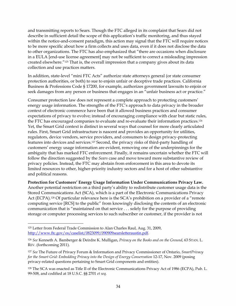
34

and transmitting reports to Sears. Though the FTC alleged in its complaint that Sears did not describe in sufficient detail the scope of this application’s traffic monitoring, and thus stayed within the notice-and-consent paradigm, this action may signal that the FTC will require notices to be more specific about how a firm collects and uses data, even if it does not disclose the data to other organizations. The FTC has also emphasized that “there are occasions when disclosure in a EULA [end-use license agreement] may not be sufficient to correct a misleading impression created elsewhere.”125 That is, the overall impression that a company gives about its data collection and use practices matters.

In addition, state-level “mini FTC Acts” authorize state attorneys general (or state consumer protection authorities, or both) to sue to enjoin unfair or deceptive trade practices. California Business & Professions Code § 17200, for example, authorizes government lawsuits to enjoin or seek damages from any person or business that engages in an “unfair business act or practice.”

Consumer protection law does not represent a complete approach to protecting customers’ energy usage information. The strengths of the FTC’s approach to data privacy in the broader context of electronic commerce have been that it allowed business practices and consumer expectations of privacy to evolve; instead of encouraging compliance with clear but static rules, the FTC has encouraged companies to evaluate and re-evaluate their information practices.126 Yet, the Smart Grid context is distinct in several ways that counsel for more clearly articulated rules. First, Smart Grid infrastructure is nascent and provides an opportunity for utilities, regulators, device vendors, service providers, and consumers to design privacy-protecting features into devices and services.127 Second, the privacy risks of third-party handling of customers’ energy usage information are evident, removing one of the underpinnings for the ambiguity that has marked FTC enforcement. Finally, it remains uncertain whether the FTC will follow the direction suggested by the Sears case and move toward more substantive review of privacy policies. Instead, the FTC may abstain from enforcement in this area to devote its limited resources to other, higher-priority industry sectors and for a host of other substantive and political reasons.

Protection for Customers’ Energy Usage Information Under Communications Privacy Law. Another potential restriction on a third party’s ability to redistribute customer usage data is the Stored Communications Act (SCA), which is a part of the Electronic Communications Privacy Act (ECPA).128 Of particular relevance here is the SCA’s prohibition on a provider of a “remote computing service [RCS] to the public” from knowingly disclosing the contents of an electronic communication that is “maintained on that service . . . solely for the purpose of providing storage or computer processing services to such subscriber or customer, if the provider is not

125 Letter from Federal Trade Commission to Alan Charles Raul, Aug. 31, 2009, http://www.ftc.gov/os/caselist/0823099/090909searsletteraustin.pdf.

126 See Kenneth A. Bamberger & Deirdre K. Mulligan, Privacy on the Books and on the Ground, 63 STAN. L. REV. (forthcoming 2011).

127 See The Future of Privacy Forum & Information and Privacy Commissioner of Ontario, SmartPrivacy for the Smart Grid: Embedding Privacy into the Design of Energy Conservation 12-17, Nov. 2009 (posing privacy-related questions pertaining to Smart Grid components and entities).

128 The SCA was enacted as Title II of the Electronic Communications Privacy Act of 1986 (ECPA), Pub. L. 99-508, and codified at 18 U.S.C. §§ 2701 et seq.

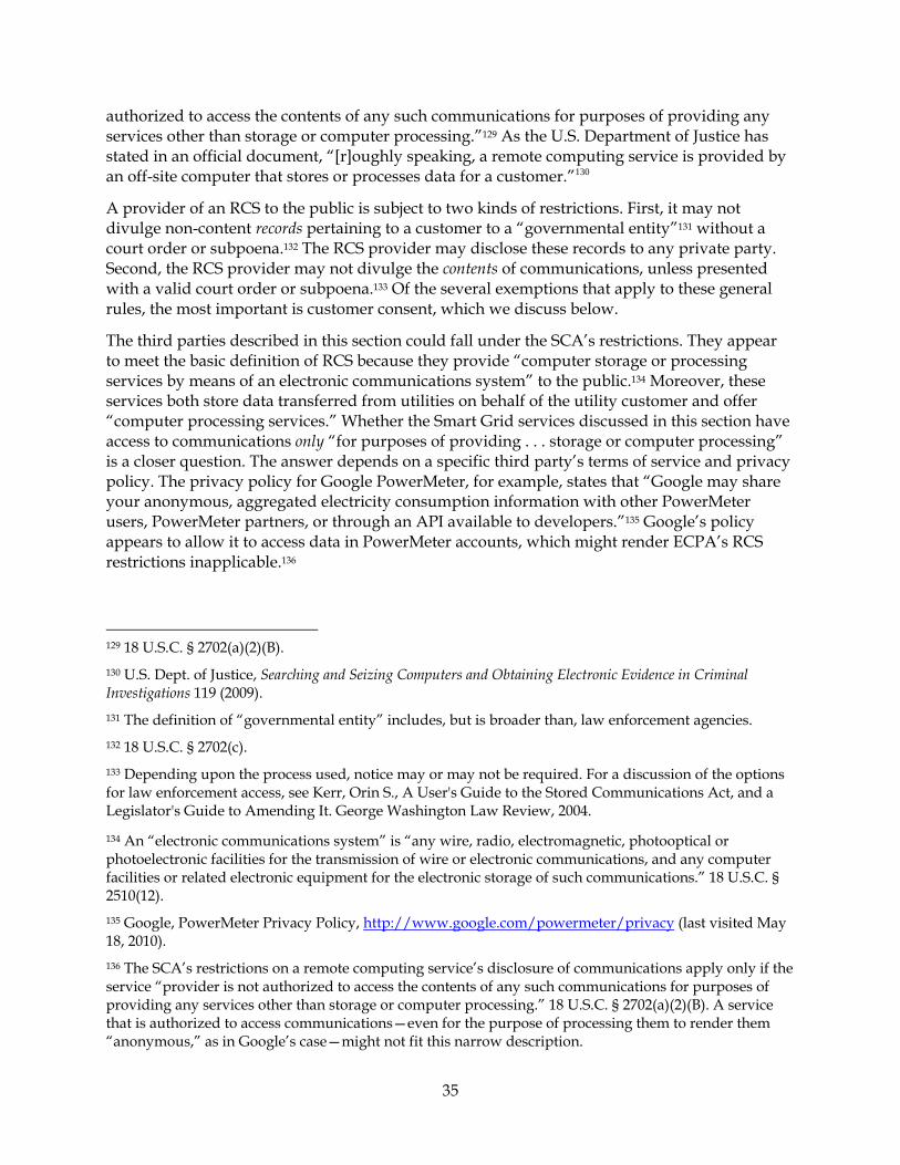
35

authorized to access the contents of any such communications for purposes of providing any services other than storage or computer processing.”129 As the U.S. Department of Justice has stated in an official document, “[r]oughly speaking, a remote computing service is provided by an off-site computer that stores or processes data for a customer.”130

A provider of an RCS to the public is subject to two kinds of restrictions. First, it may not divulge non-content records pertaining to a customer to a “governmental entity”131 without a court order or subpoena.132 The RCS provider may disclose these records to any private party. Second, the RCS provider may not divulge the contents of communications, unless presented with a valid court order or subpoena.133 Of the several exemptions that apply to these general rules, the most important is customer consent, which we discuss below.

The third parties described in this section could fall under the SCA’s restrictions. They appear to meet the basic definition of RCS because they provide “computer storage or processing services by means of an electronic communications system” to the public.134 Moreover, these services both store data transferred from utilities on behalf of the utility customer and offer “computer processing services.” Whether the Smart Grid services discussed in this section have access to communications only “for purposes of providing . . . storage or computer processing” is a closer question. The answer depends on a specific third party’s terms of service and privacy policy. The privacy policy for Google PowerMeter, for example, states that “Google may share your anonymous, aggregated electricity consumption information with other PowerMeter users, PowerMeter partners, or through an API available to developers.”135 Google’s policy appears to allow it to access data in PowerMeter accounts, which might render ECPA’s RCS restrictions inapplicable.136

129 18 U.S.C. § 2702(a)(2)(B).

130 U.S. Dept. of Justice, Searching and Seizing Computers and Obtaining Electronic Evidence in Criminal Investigations 119 (2009).

131 The definition of “governmental entity” includes, but is broader than, law enforcement agencies.

132 18 U.S.C. § 2702(c).

133 Depending upon the process used, notice may or may not be required. For a discussion of the options for law enforcement access, see Kerr, Orin S., A User's Guide to the Stored Communications Act, and a Legislator's Guide to Amending It. George Washington Law Review, 2004.

134 An “electronic communications system” is “any wire, radio, electromagnetic, photooptical or photoelectronic facilities for the transmission of wire or electronic communications, and any computer facilities or related electronic equipment for the electronic storage of such communications.” 18 U.S.C. § 2510(12).

135 Google, PowerMeter Privacy Policy, http://www.google.com/powermeter/privacy (last visited May 18, 2010).

136 The SCA’s restrictions on a remote computing service’s disclosure of communications apply only if the service “provider is not authorized to access the contents of any such communications for purposes of providing any services other than storage or computer processing.” 18 U.S.C. § 2702(a)(2)(B). A service that is authorized to access communications—even for the purpose of processing them to render them “anonymous,” as in Google’s case—might not fit this narrow description.

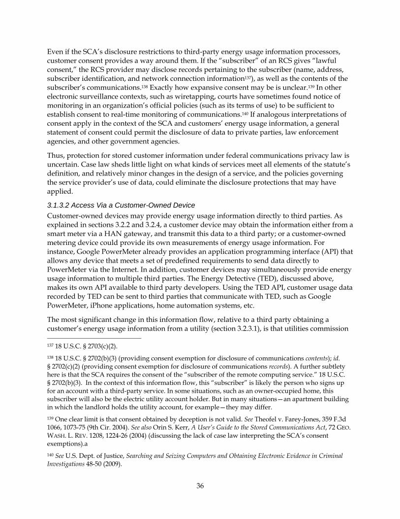
36

Even if the SCA’s disclosure restrictions to third-party energy usage information processors, customer consent provides a way around them. If the “subscriber” of an RCS gives “lawful consent,” the RCS provider may disclose records pertaining to the subscriber (name, address, subscriber identification, and network connection information137), as well as the contents of the subscriber’s communications.138 Exactly how expansive consent may be is unclear.139 In other electronic surveillance contexts, such as wiretapping, courts have sometimes found notice of monitoring in an organization’s official policies (such as its terms of use) to be sufficient to establish consent to real-time monitoring of communications.140 If analogous interpretations of consent apply in the context of the SCA and customers’ energy usage information, a general statement of consent could permit the disclosure of data to private parties, law enforcement agencies, and other government agencies.

Thus, protection for stored customer information under federal communications privacy law is uncertain. Case law sheds little light on what kinds of services meet all elements of the statute’s definition, and relatively minor changes in the design of a service, and the policies governing the service provider’s use of data, could eliminate the disclosure protections that may have applied.

3.1.3.2 Access Via a Customer-Owned Device

Customer-owned devices may provide energy usage information directly to third parties. As explained in sections 3.2.2 and 3.2.4, a customer device may obtain the information either from a smart meter via a HAN gateway, and transmit this data to a third party; or a customer-owned metering device could provide its own measurements of energy usage information. For instance, Google PowerMeter already provides an application programming interface (API) that allows any device that meets a set of predefined requirements to send data directly to PowerMeter via the Internet. In addition, customer devices may simultaneously provide energy usage information to multiple third parties. The Energy Detective (TED), discussed above, makes its own API available to third party developers. Using the TED API, customer usage data recorded by TED can be sent to third parties that communicate with TED, such as Google PowerMeter, iPhone applications, home automation systems, etc.

The most significant change in this information flow, relative to a third party obtaining a customer’s energy usage information from a utility (section 3.2.3.1), is that utilities commission 137 18 U.S.C. § 2703(c)(2).

138 18 U.S.C. § 2702(b)(3) (providing consent exemption for disclosure of communications contents); id. § 2702(c)(2) (providing consent exemption for disclosure of communications records). A further subtlety here is that the SCA requires the consent of the “subscriber of the remote computing service.” 18 U.S.C. § 2702(b)(3). In the context of this information flow, this “subscriber” is likely the person who signs up for an account with a third-party service. In some situations, such as an owner-occupied home, this subscriber will also be the electric utility account holder. But in many situations—an apartment building in which the landlord holds the utility account, for example—they may differ.

139 One clear limit is that consent obtained by deception is not valid. See Theofel v. Farey-Jones, 359 F.3d 1066, 1073-75 (9th Cir. 2004). See also Orin S. Kerr, A User’s Guide to the Stored Communications Act, 72 GEO. WASH. L. REV. 1208, 1224-26 (2004) (discussing the lack of case law interpreting the SCA’s consent exemptions).a

140 See U.S. Dept. of Justice, Searching and Seizing Computers and Obtaining Electronic Evidence in Criminal Investigations 48-50 (2009).

37

jurisdiction is tenuous. The protections—and gaps in protection—from consumer protection law and the ECPA, however, are basically unchanged.

3.1.3.3 Access Via a Third Party

Figure 5 also illustrates that energy usage information may be transferred from one third party to another. For instance, Google PowerMeter permits users to share their information with other PowerMeter users. Data sharing among third parties could become more extensive in the future. For example, a third-party collection and processing service could send energy usage information to down-stream third-party developers, such as start-up energy management companies.

As section 3.2.3.1 suggests, a primary source—and limitation—of privacy protection in this information flow is the notice that the initial third party provides to customers. The statements in these privacy policies are backed by the threat of FTC or state attorney general enforcement if notice is deficient, or actual practices deviate from the notice.

3.1.4 Energy Usage Information from Smart Meter to HAN The Smart Grid also supports the increased flow of information to individual customers. Indeed, one of the premises of state and federal Smart Grid policy is that providing customers with timely information about their energy use will lead them to use less energy or use it more efficiently. Adding price information provides a potentially powerful way of motivating customers to alter their usage patterns and enabling automated, price-responsive energy management.

Figure 5 shows how customers might acquire energy usage information in real time. The information flow in this Figure is mostly local; consumption and other data measured by the smart meter are routed through the HAN gateway to and in-home display or devices in the home. The purpose of enabling direct smart meter-to-HAN information flow is to eliminate the bottleneck that would arise from transmitting real-time information from the meter, to the utility, and then back to the customer. Smart meters can measure electricity consumption at short intervals, roughly every 10 seconds.141 Transmitting such fine-grained data to the utilities would overwhelm the capacity of their backhaul networks, but home area networks do not suffer from such severe resource constraints.142 Therefore, sending data directly from a smart meter to the HAN appears to be a more feasible way of providing customers with real-time information; but using utility backhaul networks for this purpose does not.

141 SCE, Reply Comments to Assigned Commissioner and Administrative Law Judge’s Joint Ruling Amending Scoping Memo and Inviting Comments on Proposed Policies and Findings Pertaining to the Smart Grid 14, R.08-12-009, Apr. 7, 2010, http://www.cpuc.ca.gov/EFILE/CM/115972.pdf. (“[T]he Commission also decided that it is reasonable to provide residential customers with near real-time usage data through the HAN. Accordingly, SCE, PG&E, and SDG&E have plans to provide near real-time usage data, in approximately ten-second increments, to all residential customers.”)

142 Opening Comments of Pacific Gas and Electric Company (U 39 E) on Proposed Policies and Findings Pertaining to the Smart Grid, at 15, CPUC R.08-12-009, Mar. 9, 2010 (“’Real time access’ to customer usage and pricing information can only come from localized access to such information through a Home Area Network device at the customer’s premises—not from utility ‘back office’ data collection and communication facilities.”).

38

The CPUC has granted approval for all three major IOUs to recover the cost of embedding a HAN gateway in their smart meters. When activated, the HAN gateway will route energy usage information from the smart meter to HAN devices that display electricity usage information to customers. The CPUC’s rationale for allowing HAN gateways to be part of smart meter deployment, rather than leaving it to customers to decide whether to purchase their own HAN gateway, is that “all customers should have the opportunity to use HAN devices to reduce their energy consumption,” and the “most cost effective way to provide that access, over the long term, would be through . . . meter deployment plan rather than through random retrofits.” The CPUC has scheduled the activation of the HAN gateway in smart meters to be no later than the end of 2011.143

143 CPUC Decision 09-12-046 at 65 (requiring that “each IOU be capable of providing a customer with an AMI meter with access to the customer’s usage information on a near real-time basis by the end of 2011 should the customer desire that information”).

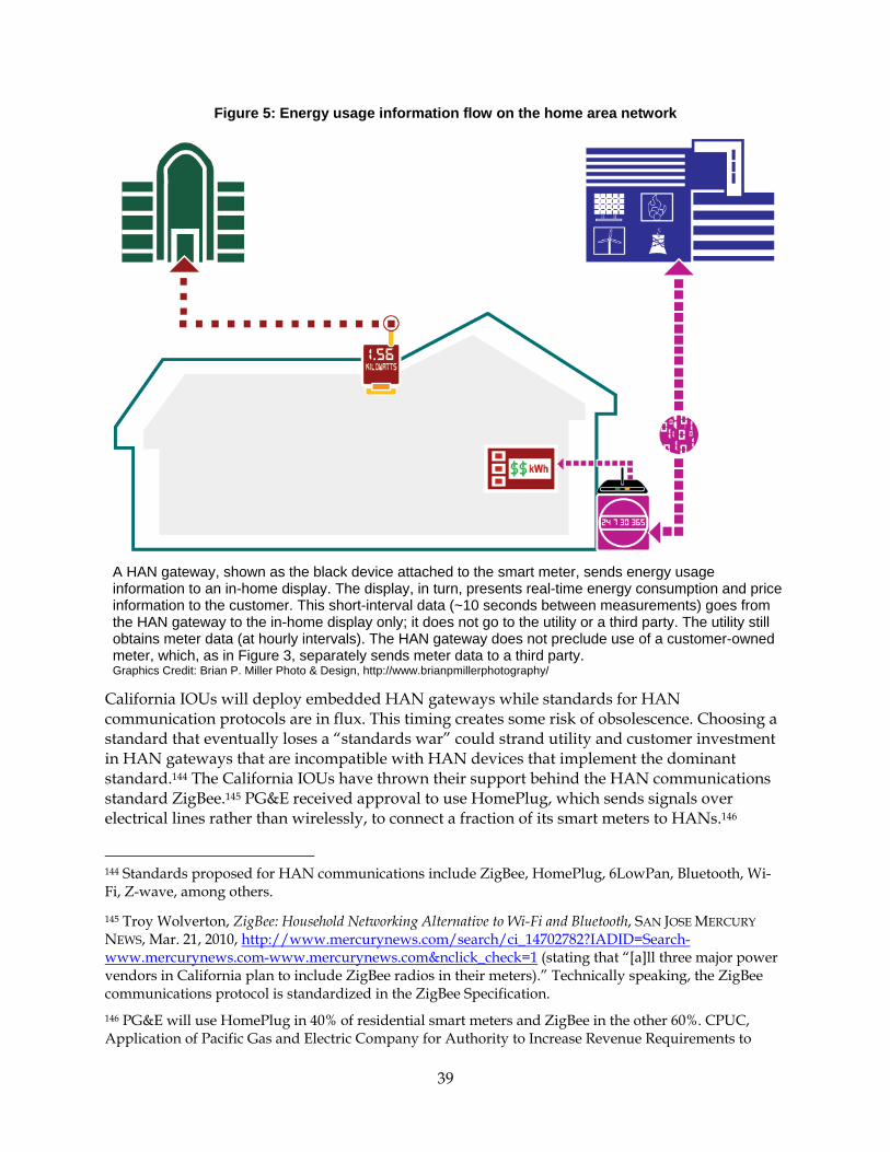
39

Figure 5: Energy usage information flow on the home area network

A HAN gateway, shown as the black device attached to the smart meter, sends energy usage information to an in-home display. The display, in turn, presents real-time energy consumption and price information to the customer. This short-interval data (~10 seconds between measurements) goes from the HAN gateway to the in-home display only; it does not go to the utility or a third party. The utility still obtains meter data (at hourly intervals). The HAN gateway does not preclude use of a customer-owned meter, which, as in Figure 3, separately sends meter data to a third party. Graphics Credit: Brian P. Miller Photo & Design, http://www.brianpmillerphotography/

California IOUs will deploy embedded HAN gateways while standards for HAN communication protocols are in flux. This timing creates some risk of obsolescence. Choosing a standard that eventually loses a “standards war” could strand utility and customer investment in HAN gateways that are incompatible with HAN devices that implement the dominant standard.144 The California IOUs have thrown their support behind the HAN communications standard ZigBee.145 PG&E received approval to use HomePlug, which sends signals over electrical lines rather than wirelessly, to connect a fraction of its smart meters to HANs.146

144 Standards proposed for HAN communications include ZigBee, HomePlug, 6LowPan, Bluetooth, Wi-Fi, Z-wave, among others.

145 Troy Wolverton, ZigBee: Household Networking Alternative to Wi-Fi and Bluetooth, SAN JOSE MERCURY

NEWS, Mar. 21, 2010, http://www.mercurynews.com/search/ci_14702782?IADID=Search-www.mercurynews.com-www.mercurynews.com&nclick_check=1 (stating that “[a]ll three major power vendors in California plan to include ZigBee radios in their meters).” Technically speaking, the ZigBee communications protocol is standardized in the ZigBee Specification.

146 PG&E will use HomePlug in 40% of residential smart meters and ZigBee in the other 60%. CPUC, Application of Pacific Gas and Electric Company for Authority to Increase Revenue Requirements to

40

Sacramento Municipal Utility District (SMUD) also plans to embed a ZigBee-compliant HAN gateway in its smart meters.147

To address the problem of incompatible HAN communication protocols that may be adopted by utility and HAN Device manufacturers, industry participants have proposed U-SNAP (Utility Smart Network Access Port) to create a protocol-agnostic and interoperable communications standard for connecting HAN Devices to smart meters.148 The first implementation of U-SNAP supports ZigBee, Z-Wave, RDS (Radio Data System), Wi-Fi and FlexNet;149 and it will likely support power line standards such as HomePlug in future implementations.150 Another solution, “Socket Interface,” is recommended by the Smart Grid Interoperability Panel Home-to-Grid Domain Expert Working Group.151 Socket Interface is “a modular appliance socket interface”152; USB, RS-232, and U-SNAP are all possible options for a Socket Interface.153 The Working Group recommends that instead of embedding a specific HAN communication protocol directly inside HAN devices, manufacturers should use the generic Socket Interface, allowing customers later to choose a communications module that is compatible with their utility’s infrastructure.154

The Smart Energy Profile 2.0 (SEP 2.0) has been identified by NIST as a standard that is applicable to HAN device communications.155 SEP 2.0 standardizes the data model for various

Recover the Costs to Upgrade its SmartMeter Program 63, D.09-03-026 (Mar. 13, 2009), http://docs.cpuc.ca.gov/word_pdf/FINAL_DECISION/98486.pdf.

147 Katie Fehrenbacher, What to Watch For in 2010: How Utilities Will Enable ZigBee, http://earth2tech.com/2009/12/29/what-to-watch-for-in-2010-how-utilities-will-enable-zigbee/ (last visited June 19, 2010). (“Sacramento Municipal Utility District’s (SMUD) Smart Meter Project Manager Erik Krause told us via email that all SMUD smart meters will use the ZigBee wireless communication.”)

148 U-SNAP, What is U-SNAP?, http://usnap.org/faqs.aspx (last visited June 19, 2010). (“U-SNAP (Utility Smart Network Access Port) is a utility industry initiative whose primary objective is to create a low-cost protocol-agnostic, interoperable communications card standard for connecting HAN (Home Area Network) devices to Smart Meters.”)

149 Id. (“The first implementations of the U-SNAP interface support ZigBee, Z-Wave, RDS (Radio Data System), WiFi and FlexNet.?”)

150 Id. (“U-SNAP modules will likely support popular power line protocols such as LonWorks and HomePlug, but further investigation is required. At a minimum, there will be U-SNAP modules that bridge to popular power-line standards.”)

151 Smart Grid Interoperability Panel Home-to-Grid Domain Expert Working Group, Free Market Choice for Appliance Physical Layer Communications, June 4, 2010, http://collaborate.nist.gov/twiki-sggrid/pub/SmartGrid/H2G/PHY-v20.pdf.

152 Id. at 2.

153 Id. at 6.

154 Id. at 2.

155 NIST, NIST Framework and Roadmap for Smart Grid Interoperability Standard, Release 1.0 57, NIST Special Publication 1108, Jan. 2010, http://www.nist.gov/public_affairs/releases/upload/smartgrid_interoperability_final.pdf. This framework document explains that the significance of being “identified” as a standard is a “stakeholder

41

HAN applications based on a set of use cases. For instance, SEP 2.0 standardizes the XML format for energy usage data transmitted from smart meters to HAN devices.156 SEP 2.0 uses IPv6 for network communications,157 and any physical network that supports IPv6 can be used to implement SEP 2.0, such as Wi-Fi, Ethernet, ZigBee, and HomePlug.158

The flow of energy usage information between the HAN gateway and the customer raises issues of privacy, innovation and openness, and security. The privacy issues arise from the fact that the devices in a home area network may transmit and store sensitive information. Transmissions may be intercepted, and hackers may break into HAN devices. The primary legal protections against these threats are the criminal laws discussed in section 3.2.1. Like communications between a smart meter and a utility, those between a HAN device and a smart meter are protected from eavesdropping by federal and state anti-wiretapping laws, so long as these devices are configured to prevent them from being made available to the general public.159 Computer fraud laws also prohibit outsiders from hacking into HAN devices that use technical mechanisms to control access. These laws, however, do not require device manufactures to provide technical protection against these threats.

Nonetheless, local routing and storage of energy usage information, such as that which could result from the HAN gateway, provides a structural constraint160 on third-party access to energy usage information. As a result, this information flow provides one way to follow the principle of data minimization, at least as far as third-party data collection is concerned. Law enforcement access illustrates the significance of this constraint. Because we presume in this example that HAN devices are located in a customer’s home, it is likely that law enforcement agents would need a search warrant either to intercept communications between a device and the smart meter or to search HAN devices for stored information.161 Wireless signals are “electronic communications;” intercepting the contents of these communications is strictly limited by the Wiretap Act’s warrant requirements.162 HAN devices, like other objects located

consensus” that the standard is applicable for some Smart Grid function(s) and supports Smart Grid interoperability. Id. at 44.

156 ZigBee Alliance and HomePlug Powerline Alliance, Smart Energy Profile 2.0 Technical Requirement Document v0.5, (Req[M-7] “the meter data structure”; Req[M-4] “simple metering data such as consumption, demand, interval data and associated measurement units shall be standardized within the profile.”).

157 Id. at 39 (“The Smart Energy 2.0 Profile will use IPv6 for network communications.”).

158 Id. at 39 (“MRD.Comm.5 -- Support all feasible physical layers (e.g., IEEE 802.15.4, 802.11, 802.39 [broadband HomePlug], forthcoming: HomePlug SE, IEEE P1901)”).

159 See 18 U.S.C. § 2511(2)(g) (exempting “intercept[ing] or access[ing] an electronic communication made through an electronic communication system that is configured so that such electronic communication is readily accessible to the general public” from the Wiretap Act’s prohibitions).

160 See Harry Surden, Structural Rights in Privacy, SMU LAW REVIEW, vol. 60, p. 1605 (2007).

161 If any of this information is transmitted to and stored by a utility or third party, however, law enforcement agents would probably be able to obtain it with a lower burden process, such as subpoena or court order.

162 See the discussion in section 3.1.2, above.

42

inside the home, are presumptively entitled to a reasonable expectation of privacy and are protected by the Fourth Amendment’s warrant requirement.

The second issue that this information flow raises is the openness of the Smart Grid to customers’ choices of HAN devices. The CPUC has authorized the major California IOUs to recover the costs of adding (predominantly) ZigBee-compliant HAN gateways to their meters, the degree to which device manufacturers produce ZigBee-compliant devices could have a large impact on privacy. Providing a large user base of ZigBee-enabled HAN gateways could lead to dominance of the ZigBee protocol and create an interoperability barrier to adopting devices that use other communications protocols.

Finally, the security model for the home area network carries privacy implications. In order to establish a secure communication between a utility-controlled HAN gateway and a customer’s HAN device, the customer may need to register the device with the utility. We explore the privacy issues surrounding device registration in section 3.3.1.

3.2 Load Management Information Privacy Risks Visions of the Smart Grid go beyond providing customers with timely, detailed information about their energy usage. Policymakers, utilities, and technology firms also envision providing the means to automate the control of devices to reduce demand and maintain grid stability. Enabling this control requires allowing devices to receive and respond to control messages, which we refer to as load management information. For example, the utility could send a signal to the controlling device letting it know the load is high. The controlling device could then cut the flow of electricity to an appliance or area of the home, according to a user’s pre-set conditions. A user could set conditions to shut off the refrigerator for one hour a day, but ensure that another appliance or area of the home remains unaffected.

As was the case with energy usage information, load management information contains details about the in-home activities that underlie energy use. Privacy risks and legal protections, as this section illustrates, also vary with the details of how HAN devices communicate with other entities.

Enabling HAN device communications inside and outside the home also raises distinct privacy, innovation, and security issues. Device-specific data streams can reveal customer behavior more clearly than aggregate energy usage information obtained from a household. Establishing secure communications will likely require device authentication, which may, in turn, require customers to register information about their devices with utilities or other entities. This step not only exposes information about the types of devices in a house to utilities and third parties, but also raises the possibility that the device registrar will become a “gatekeeper” who can control which devices may be used on a HAN.

3.2.1 Direct Utility-HAN Device Communication To begin, consider the relatively simple case of a utility communicating directly with HAN devices, as shown in Figure 6. Under current Smart Grid standards,163 a utility customer must 163 As discussed in the Introduction, efforts are currently underway to standardize Smart Grid communications protocols. The description of information flow in this section is based on HAN standards identified by NIST for implementation, including Smart Energy Profile 2.0 and OpenHAN System Requirement Specification.

43

register a HAN device with the utility in order to establish a secure communications channel between the HAN gateway at the customer’s residence and the HAN device.164 Through the HAN gateway—note that Figure 6 shows load management information going through the HAN gateway rather than the smart meter—the utility may request and obtain the status of the registered HAN device at anytime; exchange billing demand response and load control signals with the HAN device; send pricing, messaging and billing information to the customer; and monitor and control distributed energy resources at the customer’s residence. Smart Grid use cases developed by utilities envision similar information flows.165 We defer discussion of privacy issues until the details of utility-device communications are laid out in sections 3.3.1.1-5.

164 UCAIug OpenHAN Task Force, UCAIug Home Area Network System Requirements Specification v1.95 at 30, “The Registration process is a further step involving Mutual Authentication and authorizing a Commissioned HAN device to exchange secure information with other Registered devices and with an ESI.”

165 See SCE, 2006 AMI Use Cases and 2008-2009 Smart Grid Use Cases, http://www.sce.com/PowerandEnvironment/smartconnect/industry-resource-center/use-cases.htm (last visited June 20, 2010); UCAIug OpenHAN Task Force, UCAIug Home Area Network System Requirements Specification v1.95 § 4.1.

44

Figure 6: Utility-to-HAN load management information

Load management information (depicted as arrows composed of discrete circles) flows between the utility and the HAN gateway embedded in the smart meter. The HAN gateway routes load management information to devices inside the home. In effect, this architecture enables the utility to directly control HAN devices. Graphics Credit: Brian P. Miller Photo & Design, http://www.brianpmillerphotography/

3.3.1.1 HAN Device Registration

In order to register a HAN device,166 a utility customer needs to provide authentication information and detailed HAN device information to the utility.167 The HAN device information

166 The process of establishing a secure communication between a HAN gateway and a joining HAN device and enrolling the device in a utility program is given different names in different documents. UCAIug Home Area Network System Requirements Specification v1.95 describes the process as “Commissioning, Registration, Enrollment.” Smart Energy Profile Marketing Requirements Document (MRD) v1.0 (Appendix B, section1, “Installation”) uses the term “provisioning” and “registration.” Here we use “registration” to refer to the entire process of establishing a secure communication between a HAN gateway and a joining HAN device and enrolling the device in a utility program. For further details see ZigBee+HomePlug Joint Working Group, Smart Energy Profile Marketing Requirements Document (MRD) v1.0 (Appendix B, section1, “Installation”) [SEP 2.0 Marketing Requirement Document]; SCE, SmartConnect Use Case: C5 - Customer Uses Smart Appliances, http://www.sce.com/NR/rdonlyres/EC46A2AC-9D43-4674-90A7-CBE47F362CDE/0/C5_Use_Case_090105.pdf (last visited June 20, 2010) [SCE Use Case C5].

167 The California Energy Commission concluded in a 2008 report that “Customers have the right to receive price (periodic and real-time) signals and reliability signals without enrolling in utility programs and without registering their equipment with the utility.” California Energy Commission, Staff Report:

45

may include the MAC address (a unique identifier assigned to a device by the manufacturer; MAC addresses are assigned to networkable devices like Ethernet cards and printers),168 serial number, and device type, depending on the business practices of individual utilities.169 This information is provided to the utility via an out-of-band mechanism (e.g., by telephone or through a website), rather than through the channel used for smart meter communications; the utility then associates the device information with the customer’s account and uses it to establish secure communications through the utility-controlled HAN gateway. 170 For example, customers in Texas need to contact their Retail Electric Provider in order to add a HAN device, and they are limited to having five HAN devices connected to their smart meters.171 (California IOUs have not yet enabled the HAN gateways in their smart meters.)

3.2.1.2 HAN Device Tracking and Monitoring

A utility may request information from a registered HAN device via the HAN gateway at any time. The types of HAN device information that the utility may request include the device manufacturer’s name, model identifier, time and date code of manufacture, power source, etc.172 In addition, the utility may request and obtain run-time status information, such as user activity and on/off frequency of HAN devices.173

3.2.1.3 Demand Response and Load Control (DRLC)

In a DRLC event, the utility sends DRLC signals via the HAN gateway to targeted HAN devices. The DRLC signals may include event time, duration, criticality, targeted HAN device Requirements Engineering for the Advanced Metering Initiative and the Home Automation Network (AMI-HAN) Interface 4-5, Feb. 2008.

168 MAC address stands for Medium Access Control address. See MAC address, MAC address, http://en.wikipedia.org/w/index.php?title=MAC_address&oldid=370775643 (last visited June 29, 2010).

169 SEP 2.0 Marketing Requirement Document at 67 (“The Customer contacts the Utility/REP and gives the Utility/REP the HAN Device networking details (MAC Address, Installation Code) and the Customer account information.”); SCE Use Case C5 at 9-10 (“Customer contacts either the CSR or account manager in-person or by phone, or logs onto the utility’s Web site. … [HAN device] [t]ransmits device ID, device type, and cryptographic key materials to the utility over SmartConnect network via the SmartConnect Meter.”).

170 Id.

171 Smart Meter Texas, Frequently Asked Questions, https://www.smartmetertexas.com/CAP/public/home/home_faq.html#d1(last visited June 20, 2010) (“Contact your Retail Electric Provider to add HAN Devices to your account” “A Smart Meter can have up to 5 HAN Devices added.” “The information about your HAN Devices is accessible by your Retail Electric Provider.”).

172 ZigBee Alliance and HomePlug Powerline Alliance, Smart Energy Profile 2.0 Technical Requirements Document v0.5 at 71 (Req[BasicInfo-1] specifies a list of basic HAN device information and “[a]ll of the attributes shall be available via unicast requests and some [] should be available via multicast.”) [SEP 2.0 Technical Requirements Document v0.5].

173 SEP 2.0 Marketing Requirements Document at 138 (“[Utility] [s]ends a message to the HAN Device requesting the information via AMI meter [including] [c]ommunication information (e.g. log of traffic sent and received, test communication status similar to a ping of the device); [c]onfiguration information; [u]ser activity (what has been viewed and how often); On/Off frequency; [r]egistration data; HAN Device information, such as device type, model number, serial number.”).

46

IDs or categories, load adjustment offset, and event control information. The targeted HAN device is required to provide status updates to the utility at the start and end of the DRLC event, as well as any changes to the state of the device during the event that would affect anticipated energy consumption.174

3.2.1.4 Pricing, Messaging, and Billing Information

In addition to DRLC information, the utility can send pricing, messaging, and billing information to registered HAN devices. Utilities may use these kinds of messages to notify customers of upcoming grid reliability events, changes in pricing, estimated bills, and energy-saving tips.175 The utility may require the HAN devices to send back a signal to confirm the receipt of the information.176 For instance, the utility may request a specific in-home display to confirm that that a text message has been received and displayed to a consumer.177

3.2.1.5 Distributed Energy Resources (DER)

The exchange of load management information can also facilitate the integration of distributed energy resource (DER), a term that refers to energy that is generated on a small scale and close to where it is used. Solar panels on a customer’s house are a common example; others include small wind turbines and plug-in electric vehicles that supply electricity back to the grid.178 A utility can monitor and control distributed energy resources on customers’ premises.179 The relevant HAN device information required for monitoring and control includes, among other things, device state (i.e., whether it is operational, on stand-by, or down for maintenance), available capacity, and power quality.180

3.2.1.6 Privacy Issues

The privacy issues in this case are similar to those in the smart meter-to-utility information flow discussed in Part 3.1.1. Personal and account information the customer provides to the utility are likely covered by California’s security breach notification law.181 However, the MAC address

174 SEP 2.0 Technical Requirements Document v0.5 at 47 (Req[DRLC-3], “A HAN device shall provide status updates to ESI [i.e. HAN gateway] on the start and end of a DR event, and any state changes in between the period that may affect the intended energy consumption.”).

175 SEP 2.0 Technical Requirements Document v0.5 at 50 (“This provides the ability to notify Consumers of upcoming grid reliability events, changes in pricing (e.g., Time-of-Use period or next Inclining Block), energy tips, etc.”).

176 SEP 2.0 Technical Requirements Document v0.5 at 51 (Req[DM-12] Report Delivery, “ESI shall support ability to send a report of message receipts to upstream systems and deliveries upon request. Delivery date/time stamps shall be sent for each device, if message required confirmation.”).

177 ZigBee Alliance and HomePlug Powerline Alliance, Smart Energy Profile 2.0 Application Protocol Specification v0.7 at 84 (“Typically, devices which act on data obtained from servers, such as In Premises Displays or Load Controllers, will use this to indicate that a message has been obtained and acted upon, for example a TextMessage has been received and displayed to a customer.”) [SEP 2.0 Application Protocol Specification v0.7].

178 SEP 2.0 Technical Requirement Document v0.5 at 65.

179 SEP 2.0 Technical Requirement Document v0.5 at 65 (Req[DER-1] and Req[DER-2]).

180 SEP 2.0 Technical Requirement Document v0.5 at 65 (Req[DER-6]).

181 CAL. CIV. CODE § 1798.82.

47

and other HAN device-specific information are unlikely to fall within the definition of “personal information,” so this step may not subject a utility to any regulation beyond what it faces by maintaining account information. In any event, these communications and information about them are subject to the same privacy risks (government subpoenas and warrants, hackers, and civil litigant subpoenas) and protections (FTC Act, state consumer protection laws, and federal laws against wiretapping and hacking).

The level of detail in device-specific communications, however, is qualitatively different from gross energy usage measurements, even those taken at short intervals. Device-level communications could allow utilities to develop detailed profiles about which devices customers have in their homes, where they are located in relation to each other, and how and when they use them. Though this information might allow better or more accurate load forecasting, it also creates the potential for invasive marketing campaigns that could generate consumer resistance to adoption of Smart Grid technologies.182 This level of detail is similar to telephone calling records or Internet usage histories; all of these data types, when collected over time, can reveal a great deal about an individual’s (or at least a household’s) habits and activities. Yet, in contrast to phone companies and Internet service providers, which are subject to federal communications privacy laws (and, potentially, stricter state laws), utilities are subject to more varied and far less specific privacy regulations. Still, communications privacy laws do not restrict a firm’s internal use of communications records, which leaves a major source of privacy risk unaddressed. Public utilities commissions likely have the authority to regulate these detailed information flows—including internal uses by a utility—but we are not aware of any commissions that have done so.

3.2.1.7 Choice and Innovation in Devices and Services

An architecture that requires customers to register their devices with utilities could also create barriers to competition in energy management services. (Privacy is one possible dimension of competition; price and quality are others.) ZigBee Smart Energy Profile 2.0 does not require the utility to register HAN devices; the technical standard instead discusses a generic “Application Trust Center.”183 Still, this possibility in the Smart Energy Profile 2.0 provides no guarantee that utilities will choose to communicate with Application Trust Centers that they do not control. Moreover, utilities might provide financial incentives for customers to register their devices with them, even if customers may choose other registrars. For example, SDG&E has a peak time rebate schedule in effect, which offers customers with devices that can be controlled by SDG&E a bigger discount on peak-time reductions than they would otherwise receive.184

182 Smart Grid Interoperability Panel Home-to-Grid Domain Expert Working Group, Free Market Choice for Appliance Physical Layer Communications, June 4, 2010, http://collaborate.nist.gov/twiki-sggrid/pub/SmartGrid/H2G/PHY-v20.pdf (“Market tests have revealed some consumer resistance to two-way communications, particularly due to privacy concerns.”).

183 SEP 2.0 Technical Requirements Document v0.5 at 32 (stating that “[t]he Application Trust Center is responsible for authenticating and authorizing applications” and that a customer can register with multiple Application Trust Centers as well as maintain a Center).

184 SDG&E, Schedule Peak Time Rebate (filed Oct. 8, 2009). This schedule generally provides a $0.75 per kWh rebate for peak time reductions, but increases the rebate to $1.25/kWh for customers with “enabling technology,” which is defined to mean “technology which can be initiated via a signal from the Utility

48

3.2.1.8 Control of HAN Devices

Finally, direct utility control over which HAN devices individuals may connect to the network is not an inevitable consequence of the Smart Grid standards we have discussed in this section. Utilities regulators exercise some control over utility investments and other business decisions that would implement (or avoid) this model. For example, the CPUC can inquire broadly into these choices under its authority to approve or reject utilities’ requests to invest in AMI and to approve (dynamic) rates that take advantage of that infrastructure. The communication between a utility and a registered HAN device falls under the Commission’s authority to determine “just and reasonable” electric utility rates,185 and the CPUC has used ratemaking applications to set dynamic pricing schedules186 and to review utilities’ plans to adopt AMI components in conjunction with rate changes.187 These proceedings have raised a number of ratepayer protection questions, such as “[h]ow to integrate effective customer education and communication with dynamic pricing tariffs”188 and “[w]hether dynamic pricing tariffs should be voluntary, default with opt-out provisions, or mandatory.”189 Continuing attention to the details of how utilities will interact with HAN devices will help expose the privacy and control issues to public scrutiny.

3.2.2 Customer-Owned Energy Management System (EMS) The preceding discussion presumes that customers have authorized utilities to control HAN devices. A customer may also manage HAN devices through his or her own energy management system (EMS).190 Comparing Figures 6 and 7 illustrates the contrast. Whereas Figure 6 shows load management information going directly from the utility to HAN devices via the HAN gateway, Figure 7 introduces a customer-owned EMS to process and interpret

that will reduce electric energy end-use for specific electric equipment or appliances, is included in a designated Utility demand response program, and has been registered

185 CAL. PUB. UTILS. CODE §§ 451, 454; see also Cal. Code Regs. tit. 20, art. 3 (setting forth CPUC’s ratemaking procedures).

186 These proceedings are separate from, but informally related to, CPUC’s AMI proceeding (R.02-06-001) and utility applications that followed. See, e.g., Final Opinion Authorizing Pacific Gas and Electric to Deploy Advanced Metering Infrastructure 2, CPUC A.05-06-028, July 24, 2006 (recounting this history).

187 For example, CPUC is using PG&E’s application for rate revisions to set “dynamic pricing tariffs”—a necessary step to implementing demand response—by 2011. Assigned Commissioner’s Ruling and Additional Scoping Memo 8, July 25, 2006, CPUC A.06-03-005. CPUC has also reviewed utilities’ requests for rate increases to recover the cost of adding or upgrading smart meters. See, e.g., Decision on Pacific Gas and Electric Company’s Proposed Upgrade to the SmartMeter Program 3-5, Mar. 12, 2009, CPUC D.09-03-026.

188 Assigned Commissioner’s Ruling and Additional Scoping Memo 9, July 25, 2006, CPUC A.06-03-005.

189 Id. at 9. CPUC also asked whether there are “[a]ny other policy determinations that the Commission should make so that PG&E’s rate design in its 2010 GRC can address dynamic pricing tariffs in a fully integrated and comprehensive manner.” Id. at 10.

190 UCAIug OpenHAN Task Force, UCAIug Home Area Network System Requirements Specification v1.95 (Section 4.1.6 “Energy Management System”); SEP 2.0 Technical Requirements Document v0.5 at 44 (Req[C-5] PEMS Proxy, “If a “Premises Energy Management System” (PEMS) is installed, to allow customization of control messages, it must register as a HAN Device for all supported function sets with the ESI, and then act as the ESI for downstream devices and handle communications as the ESI.”).

49

commands from the utility. Under the customer-owned EMS model, the customer registers devices with the EMS and programs the EMS to respond to messages from the utility. The appliances and other HAN devices are effectively invisible to the utility, though the EMS is not.191

191 SCE, SmartConnect Use Case: C6-Customer Uses an Energy Management System (EMS) or In-Home Display (IHD) at 18, http://www.sce.com/NR/rdonlyres/C39473B2-50BF-48C6-BAC7-4904DEE0D51F/0/C6_Use_Case_090105.pdf (last visited June 20, 2010) (“[The EMS] [e]xecutes programmed response for one or more associated HAN devices to reduce or limit load at customer’s premises, based on customer preferences configured into EMS” and “[a]ssumes the customer takes responsibility for device registration with EMS and the utility has no visibility to downstream devices.”).

50

Figure 7: Load management information flows with a customer-owned EMS

A customer-owned energy management system (EMS) (depicted as a computer keyboard and screen) routes load management information between the HAN gateway and HAN devices. The HAN gateway, in turn, routes load management information between the home and the utility. HAN devices are registered with the EMS rather than the utility. Graphics Credit: Brian P. Miller Photo & Design, http://www.brianpmillerphotography/

The EMS market is nascent but developing rapidly. Device manufacturers have produced proof-of-concept prototypes. For instance, General Electric has introduced an energy information panel that can wirelessly connect to a smart meter and HAN devices via Wi-Fi or ZigBee in order to gather information, control devices, and recommend ways to save energy.192 Intel introduced an Intelligent Home Energy Management Proof of Concept that can wirelessly connect a smart thermostat and appliances, and allows remote viewing and control of these

192 General Electric, GE Smart Home-Energy Panel Tells Consumers What’s Happening with Their Power Profile, http://www.gepower.com/about/press/en/2010_press/010810.htm (last visited June 20, 2010) (“The panels even will be able to be programmed to control smart appliances, thermostats and heating and cooling devices.”).

51

devices.193 Finally, NIST identified several EMS-related standards for implementation or further study.194

Compared with direct utility-HAN device communication, a customer-controlled EMS provides several privacy safeguards. First, it exposes less information about the home to the utility. Because the HAN devices are not registered with or controlled by the utility, the detailed HAN device information is invisible to the utility. If a customer-owned EMS does not route HAN communications outside the home, then utilities and third parties will not routinely have access to detailed customer usage data.195 This is one way that a customer-controlled EMS permits more customer choice over the actions of their HAN devices in a utility event, which could produce more load response and greater customer satisfaction.196 One potential disadvantage is that buying and maintaining an EMS may be more expensive and time-consuming than granting control of HAN devices to utilities or third parties for energy management.

The major risks to privacy come from malicious actors who may seek to intercept wireless communications or penetrate the HAN via an Internet connection. As previously discussed, encryption and other technical measures, as well as criminal laws that prohibit eavesdropping and hacking are the main forms of protection against these threats.

3.2.3 Third-Party Energy Management Systems A third possibility for energy management is to have a third party provide the service. As shown in Figure 8, a customer could use a non-utility third party service to control HAN devices’ in response to signals from utilities or the customer. These third parties may remotely administer home area networks either over the Internet or through a utility’s AMI network.

Internet-based, third-party energy management services would bypass utilities. Intamac Systems, a U.K.-based company, is already offering home energy management services over broadband and cloud-computing platforms to homes in U.K. and Australia; the service goes

193 Intel, Intel Intelligent Home Energy Management Proof of Concept, http://www.intel.com/embedded/energy/homeenergy/323157.pdf (last visited June 20, 2010).

194 Standards related to EMS identified by NIST for implementation or further review include ZigBee Smart Energy Profile 2.0 (specifying the requirements for Premise Energy Management System), OpenHAN (including EMS use cases), IEC 61968/61970 Suites (defining application-level EMS interfaces and messaging for distribution grid management), and ISO/IEC 15067-3 (defining a model of an energy management system for the home electronic system). NIST, NIST Framework and Roadmap for Smart Grid Interoperability Standard, Release 1.0, at 50-73, NIST Special Publication 1108, Jan. 2010.

195 But utilities will still have access to customer usage data measured by smart meters.

196 CEC, Proposed Load Management Standards (Draft Committee Report) 27, CEC-400-2008-027-CT (Nov. 2008), http://www.energy.ca.gov/2008publications/CEC-400-2008-027/CEC-400-2008-027-CTD.PDF (last visited June 19, 2010) (“The Statewide Pricing Pilot and other similar pilots have clearly demonstrated that ’customer choice’ produces significantly more load response and much greater customer satisfaction than utility control. With customer choice, the customer, not the utility, determines what loads to control, and when, if, and how much to control those loads.”); E. Koch, Akuacom and M.A. Piette, Direct versus Facility Centric Load Control for Automated Demand Response at 7, http://drrc.lbl.gov/pubs/lbnl-2905e.pdf (last June 20, 2010) (stating that direct load control is more predictable, but an EMS has “the potential to present a more reliable response to a DR signal” because it can manage multiple resources to respond).

52

beyond monitoring energy usage, but controls individual devices in customer’s homes via broadband.197 Energy management companies in the U.S. are also actively working with Internet service providers to offer similar services.198 This model might be attractive as HAN devices become popular, because it could enable customers to set the policies that their devices will follow but leave the details of administering devices to a third party.

Alternatively, a third-party energy management service provider may operate through utilities’ AMI networks. There is no commercial product or service for this information flow yet, but it has been discussed in at least one utility Smart Grid use case.199 In this information flow, a customer provides the utility with the unique identifier of the HAN device to which he or she wishes to enable third-party access and control. The utility then authenticates the customer and the third-party and, if this is successful, the utility sends the identifier to the third party. The third party may then control the HAN device through the utility’s AMI network.200 However, due to load and latency issues with utilities’ AMI networks,201 the viability of this information flow remains unclear.

The privacy risks discussed in section 3.3.1—exposing information about individual device usage and the underlying household activities—also apply to this information flow. The difference here is that public utilities commission regulatory authority is tenuous. If a non-utility energy management service provider obtains data from a utility, a commission might be able to require the utility to put privacy safeguards in contracts or service agreements with the provider. If customers send data directly to the energy management service provider, however, a utilities commission may not have, or be unwilling to exercise, jurisdiction over the provider.

197 Intamac, The Dawn of Smarter Energy?, http://www2.intamac.com/blog/the-dawn-of-smarter-energy.html (last visited June 20, 2010) (“Using the Intamac web platform consumers can not only monitor the overall energy usage at their home, but control individual devices and program the service to intelligently act on their behalf.”).

198 Jeff St. John, Intamac Gets £4M for Home Energy Cloud Computing, http://earth2tech.com/2010/06/16/intamac-gets-4m-for-home-energy-cloud-computing/ (last visited June 20, 2010) (stating that U.S.-based such as OpenPeak and iControls are working with telecoms such as AT&T to offer energy management service over broadband); Jeff St. John, The Telco Home Energy Invasion, http://www.greentechmedia.com/articles/read/the-telco-home-energy-invasion/, (last visited June 20, 2010) (stating that Verizon and AT&T were both making moves to bring home energy platforms to their customers).

199 SCE, AMI Use Case: C4 - External clients use the AMI to interact with devices at customer site, http://www.sce.com/NR/rdonlyres/EBE21A86-4975-48D3-AEF7-573EDDDB68D8/0/ARCHC4USECASEv13060627.pdf (last visited June 20, 2010).

200 Id.

201 Smart Grid Interoperability Panel Home-to-Grid Domain Expert Working Group, Free Market Choice for Appliance Physical Layer Communications at 4 (June 4, 2010), http://collaborate.nist.gov/twiki-sggrid/pub/SmartGrid/H2G/PHY-v20.pdf (last visited June 20, 2010) (explaining the load and latency problems with AMI systems when large quantities of customers participate in demand response or when real time communication is required).

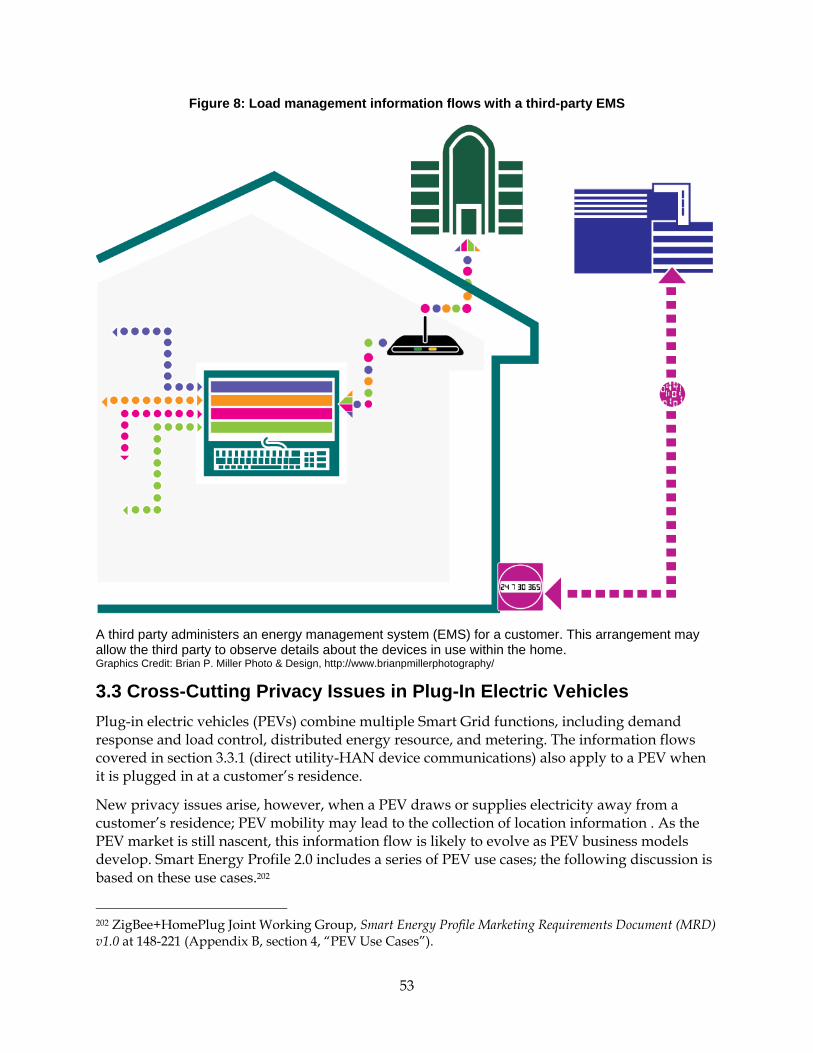
53

Figure 8: Load management information flows with a third-party EMS

A third party administers an energy management system (EMS) for a customer. This arrangement may allow the third party to observe details about the devices in use within the home. Graphics Credit: Brian P. Miller Photo & Design, http://www.brianpmillerphotography/

3.3 Cross-Cutting Privacy Issues in Plug-In Electric Vehicles Plug-in electric vehicles (PEVs) combine multiple Smart Grid functions, including demand response and load control, distributed energy resource, and metering. The information flows covered in section 3.3.1 (direct utility-HAN device communications) also apply to a PEV when it is plugged in at a customer’s residence.

New privacy issues arise, however, when a PEV draws or supplies electricity away from a customer’s residence; PEV mobility may lead to the collection of location information . As the PEV market is still nascent, this information flow is likely to evolve as PEV business models develop. Smart Energy Profile 2.0 includes a series of PEV use cases; the following discussion is based on these use cases.202

202 ZigBee+HomePlug Joint Working Group, Smart Energy Profile Marketing Requirements Document (MRD) v1.0 at 148-221 (Appendix B, section 4, “PEV Use Cases”).

54

To enroll a PEV in utility programs, the customer contacts the utility and provides the PEV ID (e.g., the vehicle identification number), along with other authentication information of the customer. The utility authenticates the customer, and records the PEV information in its internal database.

Each time the customer charges the PEV, the PEV ID, an identifier for the charging location (named Premises ID in SEP 2.0), and other information pertaining to the electric charging session are transmitted to the utility. In order to bill the electricity charging to the proper customer account, the utility first checks PEV ID and Premises ID in its internal database. If the PEV ID and Premises ID are found, the cost is charged to the Customer’s account. If the PEV ID and Premises ID are not found (i.e., the PEV is enrolled in a different utility), the PEV ID is forwarded to a clearinghouse to identify the utility that the PEV is enrolled in. The clearinghouse might store the PEV ID and Premises ID, but the current standard is unsettled as to whether the clearinghouse will store information or merely act as a channel for information exchange. If the PEV is enrolled in any utility, the cost of the charging is forwarded to the enrolled utility via the clearinghouse. Otherwise, the PEV begins charging based on the customer’s selected preferences.

55

Figure 9. Information flows from plug-in electric vehicle charging

A plug-in electric vehicle (PEV) travels from northern to southern California. The PEV is charged along the route at a charging station and at the final destination. During both charging sessions, energy usage information is cleared through a clearinghouse in order to bill the customer for the electricity he uses to charge his vehicle. Graphics Credit: Brian P. Miller Photo & Design, http://www.brianpmillerphotography/

PEVs introduce a privacy interest that is distinct from those discussed so far in this report: a customer’s location outside the home. Location information has obvious appeal to law enforcement agencies as well as civil litigants (e.g., a spouse seeking evidence of where his or her spouse has traveled during a divorce). As with other kinds of Smart Grid data, public utilities commissions can probably create privacy rules for PEV-related data that utilities collect; but third parties are probably outside commissions’ jurisdictions.

Moreover, PEV mobility means that a customer might deal with many different third parties. A customer who drives from northern to southern California (as shown in Figure 9) would begin and end his trip in different IOUs’ service territory. A stop at a charging station along the way introduces a third party to the information flow. As a result, the work that the customer must do to understand how data about his location and his PEV is handled during the trip multiplies.

56

Travel across state lines further complicates this situation, as different states might have different privacy rules concerning PEVs. Another interstate element is the possibility that the clearinghouse for PEV information is located in a different state, as is the case in Figure 9.

Statutes that protect motor vehicle records, such as the Drivers Privacy Protection Act (DPPA)203 and similar state laws—are unlikely to constrain either the in-state or out-of-state data flows depicted in Figure 9. The DPPA applies to disclosures of “personal information” by state motor vehicle departments, not the private parties discussed here.204 States may extend the DPPA’s baseline protections to cover more entities and more types of information, but this would leave the problem of inconsistent state protections. In the end, PEVs illustrate the need for a more comprehensive approach to Smart Grid data privacy.

203 18 U.S.C. § 2721 et seq.

204 See 18 U.S.C. § 2721(a) (establishing prohibitions for a “State department of motor vehicles, and any officer, employee, or contractor thereof”); Reno v. Condon, 528 U.S. 141, 144 (2000) (“The DPPA establishes a regulatory scheme that restricts the States' ability to disclose a driver's personal information without the driver's consent.”).

57

CHAPTER 4: Conclusions and Recommendations 4.1 Conclusions With vigorous state and federal support, the Smart Grid is rapidly taking shape. Although many details remain to be decided about the technical capabilities of Smart Grid components and how the Smart Grid will support broader energy policy goals in California and elsewhere, California has made a substantial investment—in terms of policy commitments and ratepayer resources—to a Smart Grid that will allow utilities to collect detailed information about residential customers’ energy use, and that may allow third parties to collect far more detailed information.

This integration of information technology with the electric grid holds great potential for helping customers make better-informed decisions about their energy use. It may also serve to make the grid more reliable and resilient, reduce the growth in demand for electricity, and incorporate renewable and distributed energy sources. How utilities, regulators, and other stakeholders will make use of this data to achieve these goals is an area that deserves further exploration. Regardless, the technology and data flows pose challenges to privacy protection that require attention to the architecture and information flows of the Smart Grid as well as the adoption of new laws and policies and the expansion of those already on the books.

4.2 Recommendations It is evident that the collection, use, and disclosure of Smart Grid data present considerable risks to individual privacy. One lesson from the rise of the commercial Internet, , as well as the integration of information technology into domains ranging from copyright205 to healthcare, is that information practices that violate individuals’ privacy expectations are likely to generate customer backlash and loss of trust. The Smart Grid is no different.

This report emphasizes that policymakers, utilities, and technology firms can adopt a systematic approach to identifying and assessing the privacy risks associated with Smart Grid deployments by analyzing information flows alongside general information privacy frameworks (e.g., FIPs) and applicable state and federal information privacy laws. Though the details of the information flows that we examined may change, and other information flow patterns will undoubtedly emerge, the approach developed in this report is adaptable to these variations.

The recommendations that we offer below are based on two overarching findings. First, the Smart Grid creates new types of data that implicate individual privacy. These data types may reveal a great deal about individual behavior but receive little or no legal protection. HAN

205 For analysis of how rapid technological change met consumer resistance for its failure to accommodate existing legal and social norms, see Deirdre Mulligan & Aaron Burstein, Implementing Copyright Limitations in Rights Expression Languages, in Proceedings of the 2nd ACM Workshop on Digital Rights Management Systems (2002); Deirdre Mulligan, John Han & Aaron Burstein, How DRM-Based Content Delivery Systems Disrupt Expectations of “Personal Use,” in Proceedings of the 3rd ACM Workshop on Digital Rights Management Systems (2003).

58

device registration and communication information, location, and information associated with each charging plug-in electric vehicles are examples of Smart Grid data that may outstrip the definitions of private data under current laws and regulations.

Second, current privacy laws and regulations apply to a narrow slice of Smart Grid data and, even then, they treat different Smart Grid actors inconsistently. Some data pertaining to energy usage is clearly within the scope of established privacy law rules and regulators, while similar data collected from a different source might be subject to far less certain protection. For example, a utility and a third-party energy management service face starkly different regulatory landscapes, even though they may control and process similar data. Moreover, the laws that do protect electricity usage data generally offer lower levels of protection than privacy laws designed for data of similar sensitivity, such as telephone and Internet usage records. Establishing privacy rules that apply equally to data of similar sensitivity, irrespective of whether a utility or a third party controls the data, would help eliminate regulatory arbitrage and reduce customer confusion. Maintaining protections that are reasonably consistent with those that shielded customer privacy in the pre-Smart Grid electricity environment requires immediate action.

We recommend the following steps to help provide privacy protections that are consistent with customer expectations:

Privacy considerations must drive architectural and information flow design decisions within the network, as well as the policies that cover Smart Grid data held by the growing array of entities that will help reap the benefit of this investment. Because privacy must be embedded in technical design, it cannot be addressed adequately by policies that created once technologies have matured.

Because privacy risks are fairly consistent across jurisdictions, and the markets for Smart Grid technologies are national, federal policymakers should take the lead in setting legal and technical requirements to protect privacy. NIST, FERC, and the Department of Energy should recognize that the rules, standards, and guidance they develop will determine a great deal about how the Smart Grid develops. They should take advantage of this position to protect privacy.

Recognizing that the smart grid raises privacy concerns due to the lack of consistent privacy rules for similarly situated players and the expanding amount of data they will have access to, and that federal action is unlikely to adequately address these concerns, we recommend that states act to address these gaps. State utilities regulators (such as the California Public Utilities Commission) should use their institutional expertise in protecting consumer interests and their broad authority to protect privacy through administrative rules and technical requirements. Both regulatory mechanisms have roles to play in protecting privacy.

Privacy issues are not entirely separate from grid cybersecurity and issues of keeping the grid open to innovative devices and services. Regulators at all levels therefore should not consider them in isolation but rather use rulemakings and rate case proceedings to take the interdependencies among these issues fully into account.

The utilities and technology firms that are building the Smart Grid should also protect privacy through their design and implementation of hardware, software, and services.

59

Consumer protection and civil liberties groups should continue to engage with federal and state Smart Grid policy proceedings as well as standard-setting efforts to ensure that the technical and policy blueprints for the Smart Grid protect individual privacy.

Widely accepted information privacy frameworks, such as the Fair Information Practices, serve as a useful starting point and should provide the foundation for all Smart Grid players to engage on privacy issues.206

4.3 Benefits to California We hope that this report will be useful to technology companies, utilities, and policymakers as they identify privacy issues in the Smart Grid and reconcile privacy protections with other energy policy goals. Moreover, our approach of combining technical and legal analysis clarifies the issues that state and federal guidelines, standards, and regulations can helpfully address. We have shared elements of this report throughout its development with audiences that include policymakers, technologists, and academics. For instance, parts of this report were presented at a conference on climate change and the future of energy at the University of Toledo School of Law in March 2010 and an i4Energy Center207 seminar at UC Berkeley in April 2010. In addition, we submitted public comments on privacy, cybersecurity, and innovation issues to the CPUC on several occasions during its Smart Grid rulemaking; and we submitted a public comment to NIST and the White House Office of Science and Technology Policy (OSTP) in response to OSTP’s request for public comment on the consumer interface with the Smart Grid.208

206 For a Fair Information Practice Principle based approach to Smart Grid privacy see, “Joint Comments of the Center for Democracy & Technology and the Electronic Frontier Foundation on Proposed Policies and Findings Pertaining to the Smart Grid,” before the California Public Utilities Commission in the Assigned Commissioner and Administrative Law Judge’s Joint Ruling Amending Scoping Memo and Inviting Comments on Proposed Policies and Findings Pertaining to the Smart Grid 33-39 (Feb. 8, 2010) (March 9, 2010).

207 The i4Energy Center’s mission is “to facilitate and promote research on system-integrated enabling technologies that will achieve better energy efficiency, improved demand/response, and dramatic improvements in energy distribution.” i4Energy, Mission Statement, http://i4energy.org/mission-statement (last visited June 29, 2010).

208 75 Fed. Reg. 7526, Feb. 19, 2010.

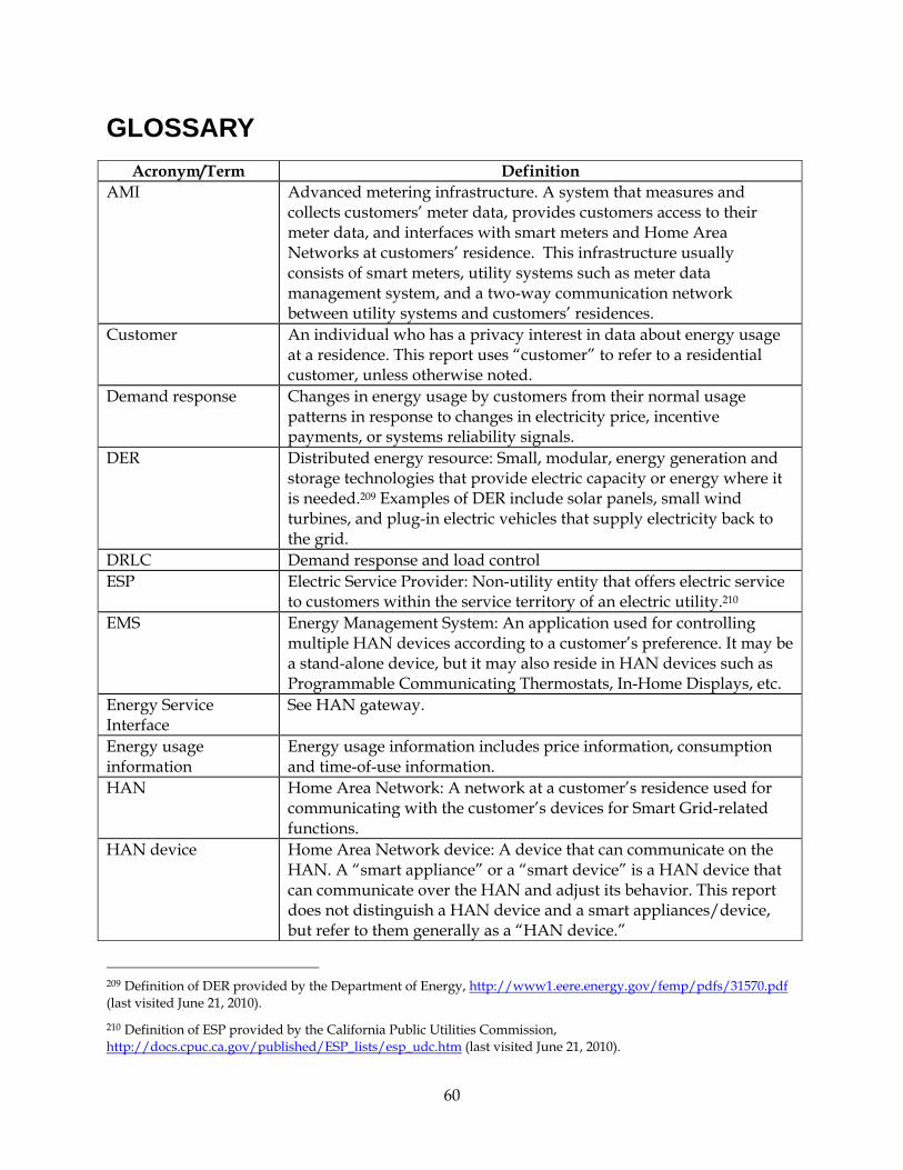
60

GLOSSARY Acronym/Term Definition

AMI Advanced metering infrastructure. A system that measures and collects customers’ meter data, provides customers access to their meter data, and interfaces with smart meters and Home Area Networks at customers’ residence. This infrastructure usually consists of smart meters, utility systems such as meter data management system, and a two-way communication network between utility systems and customers’ residences.

Customer An individual who has a privacy interest in data about energy usage at a residence. This report uses “customer” to refer to a residential customer, unless otherwise noted.

Demand response Changes in energy usage by customers from their normal usage patterns in response to changes in electricity price, incentive payments, or systems reliability signals.

DER Distributed energy resource: Small, modular, energy generation and storage technologies that provide electric capacity or energy where it is needed.209 Examples of DER include solar panels, small wind turbines, and plug-in electric vehicles that supply electricity back to the grid.

DRLC Demand response and load control ESP Electric Service Provider: Non-utility entity that offers electric service

to customers within the service territory of an electric utility.210 EMS Energy Management System: An application used for controlling

multiple HAN devices according to a customer’s preference. It may be a stand-alone device, but it may also reside in HAN devices such as Programmable Communicating Thermostats, In-Home Displays, etc.

Energy Service Interface

See HAN gateway.

Energy usage information

Energy usage information includes price information, consumption and time-of-use information.

HAN Home Area Network: A network at a customer’s residence used for communicating with the customer’s devices for Smart Grid-related functions.

HAN device Home Area Network device: A device that can communicate on the HAN. A “smart appliance” or a “smart device” is a HAN device that can communicate over the HAN and adjust its behavior. This report does not distinguish a HAN device and a smart appliances/device, but refer to them generally as a “HAN device.”

209 Definition of DER provided by the Department of Energy, http://www1.eere.energy.gov/femp/pdfs/31570.pdf (last visited June 21, 2010).

210 Definition of ESP provided by the California Public Utilities Commission, http://docs.cpuc.ca.gov/published/ESP_lists/esp_udc.htm (last visited June 21, 2010).

61

HAN gateway Home Area Network gateway: A gateway device through which a customer’s HAN communicates with the customer’s utility or any other entity that provides energy management services. A customer may have multiple HAN gateways on the customer’s premise, and the same HAN device may communicate with multiple HAN gateways. Although HAN gateways are embedded in smart meters by major California utilities, HAN gateways and smart meters are logically separate; a HAN gateway can be a stand-alone device, integrated with a HAN device, or embedded in a smart meter. The HAN gateway is also known as Energy Service Interface (ESI).

IOU Investor-owned utility. See Utility Load management information

Load management information includes price and event signals from utilities, control traffic exchanged among HAN devices and the systems and entities that control them, and HAN device identification and authentication information.

MAC address Media access control address: A unique identifier for a network interface device. For example, Ethernet interfaces have 48-bit MAC addresses.

Meter data Any data collected by an electric meter, such as the consumption and time-of-use information, quality of service data, communications configurations, and security-related data. If HAN gateways are embedded in smart meters, meter data only refers to the data associated with metering function of the smart meters, excluding the data associated with HAN function of the smart meters.

Smart appliance/device

See HAN device.

SEP 2.0 Smart Energy Profile 2.0: A standard developed by ZigBee Alliance and HomePlug PowerLine Alliance that defines communications and information model for HAN devices. It has been identified by National Institute of Standards and Technology as one of the Smart Grid standards for implementation.

Use case Description of the interaction of different actors (customers, utilities, and others), and the functional requirements to implement these interactions within the Smart Grid.

POU Publicly owned utility. See Utility. Utility In this report a utility refers to a vertically integrated utility from the

perspective of residential customers in California. This report does not consider the different types of service providers in a restructured retail electricity market. Based on types of ownership, utilities are categorized into investor-owned utility (IOU), publicly owned utility (POU), and cooperative utility. The IOUs are private corporations; the authority of state Public Utility Commission (PUCs) is often limited to the IOUs. POUs are owned by municipal, state, or federal governments; POUs are self-

62

regulated by their governing boards and are generally not subject to state or federal economic regulation.

63

APPENDIX A: CPUC Decisions Approving Residential AMI Investments This table is compiled from the CEC’s Proposed Load Management Standards (Draft Committee Report)211 , CPUC decisions approving IOUs’ AMI investments,212 and utility website.213

PG&E SDG&E SCE

CPUC decision D. 06-07-027

(original plan in 2006)

D. 09-03-026 (update in 2009)

D. 07-04-043 D. 08-09-039

Communication network

PLC for its electric;

RF for gas

RF mesh RF mesh RF mesh

Customer access to meter data

Internet Access

Internet access + HAN

Internet access + HAN

Internet access + HAN

15-minute data for commercial and industrial customers

Yes Yes Yes Yes

Hourly data for residential customers

Yes Yes Yes Yes

Two-way communication

Yes Yes Yes Yes

Remote updatability

No Yes Yes Yes

211 Calif. Energy Comm’n, Proposed Load Management Standards (Draft Committee Report) 27, CEC-400-2008-027-CT (Nov. 2008), http://www.energy.ca.gov/2008publications/CEC-400-2008-027/CEC-400-2008-027-CTD.PDF (last visited June 19, 2010). See in particular pp. 23-25 (summarizing AMI implementation as of November 2008).

212 CPUC Decision 09-03-026 (HAN gateway in PG&E Smart Meter has both ZigBee and HomePlug connection); CPUC, Demand Response and Advanced Metering, http://www.cpuc.ca.gov/PUC/energy/Demand+Response/R0206001.htm (last visited June 20, 2010) (list of decisions approving IOUs’ deployment plans).

213 PG&E, New Technologies, http://www.pge.com/about/news/mediarelations/newsimages/newtech/ (last visited June 20, 2010) (PG&E employs RF Mesh network).

64

Physical interface of HAN Gateway

No ZigBee and HomePlug

ZigBee ZigBee

65

APPENDIX B: Major HAN Communication Protocols The features of these HAN communication protocols can be summarized in the table below:214

Protocol Wired/Wireless One/Two way

Openness

ZigBee Wireless Two way Private, available to license holders.

HomePlug Wired, power line communication

Two way Private, available to license holders.

6LowPan Wireless Two way IETF standard

Bluetooth Wireless Two way IEEE standard

Wi-Fi Wireless Two way IEEE standard

Z-wave Wireless Two way Private, available to license holders.

214 Charles McParland, Home Network Technologies and Automating Demand Response at 19, http://drrc.lbl.gov/pubs/lbnl-3093e.pdf (last visited June 20, 2010).

APPENDIX Q Appendix Q: Appendix 10: People and Energy at Home

2087 Addison Street, 2nd Floor Berkeley, CA 94704-110

(510) 643-1440 uc-ciee.org

California Institute forEnergy and Environment

People and Energy at Home: Information Display and Thermal Comfort Development for Residences

Final Project Report April 26, 2012 Prepared by Therese Peffer, Ph.D., CIEE Professor Edward Arens, CBE and Dept of Architecture, UC Berkeley Professor David Auslander, Dept of Mechanical Engineering, UC Berkeley Prepared for CIEE Enabling Technology Development Program Program Manager(s) Gaymond Yee Subaward: PODR01:B09

Table of Contents 

1 ExecutiveSummary...............................................................................................................................2

2 Introduction.............................................................................................................................................2

3 Background...............................................................................................................................................33.1 InformationDisplay.......................................................................................................................................33.2 ResidentialThermalComfort.....................................................................................................................4

4 ResearchDesign......................................................................................................................................64.1 InformationDisplay.......................................................................................................................................64.2 ResidentialThermalComfort.....................................................................................................................6

5 Results........................................................................................................................................................65.1 InformationDisplay.......................................................................................................................................65.1.1 Summaryoftheoutlineofpsychographictoolsandotherevaluationtools..................65.1.2 ExistingIn‐HomeEnergyDisplay.....................................................................................................95.1.3 Evaluationofweb‐baseddisplays.................................................................................................10

5.2 ResidentialThermalComfort..................................................................................................................155.2.1 Surveydatareview..............................................................................................................................155.2.2 Algorithmsdeveloped........................................................................................................................255.2.3 Tests...........................................................................................................................................................27

6 Recommendations................................................................................................................................296.1 InformationDisplay....................................................................................................................................296.1.1 Targetingdisplays................................................................................................................................29

6.2 ThermalComfort..........................................................................................................................................31

7 References...............................................................................................................................................32

8 Appendix1:DevelopingtheAdaptiveThermostatAlgorithm.............................................358.1.1 Developingthealgorithm.................................................................................................................368.1.2 Advicegenerationtoengageenergysavingbehavior...........................................................43

2

1 Executive Summary  This research covered two subjects: one study examined what types of information and motivation would encourage people to reduce their energy consumption using an information display and the other researched different thermostat control strategies to achieve an acceptable thermally comfortable home while also reducing energy used by heating and cooling systems. The impetus was to provide an application of distributed wireless sensors and microprocessors to provide a low-cost infrastructure towards improving residential thermal comfort and reducing electricity consumption through more detailed feedback, especially during peak times. The research regarding in-home energy displays involved exploring psychographic segmentation, reviewing existing displays, evaluating three displays in detail, and suggesting three types of display for three segments of the population. The various psychographic segmentations had commonalities—people motivated by money, the environment, and peers were the three targeted populations chosen. For each segment was described the type of information (e.g., cost, carbon emissions related to energy consumption) as well as the type of display (e.g., numeric versus graphic. In addition, common attributes that all displays might share were discussed, such as more granular level of data (e.g., appliance level) and high latency. The thermal comfort research included reviewing several existing surveys regarding how people use thermostats, developing and administering a separate survey, and developing and testing algorithms. Both surveys pointed out commonly used means of control that are outside the purvue of typical thermostatic control, such as using the off switch, override, and hold modes. The open-ended questions of the survey created provided other insights into what people want and don’t want in thermostatic control, as well as lent support to increasing thermal variability in the home. Respondents reported thermal comfort related to physical measures (e.g., house construction), certain behaviors, and especially social issues (age, gender, schedules). The functions reported not used fell in four general categories: those not used because not needed, because it was not applicable, because it didn’t work well, and because the user did not know how to use it. The algorithm developed provided setpoints that adapt to outdoor air temperature and relative humidity; initial simulation testing showed that this has promise of providing the seasonal and daily variability that survey responders recognized—and save energy and money in the process. The algorithm could be improved in many ways, not the least would be to test in the field. Other issues of improving thermostats included more usable interfaces and other features such as timers and occupancy sensors.

2 Introduction Residential buildings in California consume one third of the state’s electricity and are responsible for about one fifth of the state’s carbon emissions. However, residents typically have no feedback on their electrical consumption except for the monthly utility bill. Current sensors on appliances throughout the house can supply real-time energy usage information. This information, however, requires careful processing and management in order to be useful to people.

3

Heating and cooling homes consume a substantial portion of both fuel and electrical energy—9% of the total energy consumption in the U.S. (Peffer et al. 2011); residential air conditioning alone accounts for 14% of the typical peak electrical load in California (Borenstein, Jaske, & Rosenfeld 2002). Yet there is surprisingly little current research on residential thermal comfort. The Programmable Communicating Thermostat (PCT) and more recently the Upgradable Setback Thermostat (UST) have been promoted for residential Demand Response programs, yet it is unclear what type of information—much less motivation—will encourage people to make better choices about their electricity consumption. Distributed temperature sensors and online weather forecasting information can provide better control over the heating, cooling, and ventilation systems in a house. This study is two-fold. We studied different types of people to understand what types of information and motivation might encourage them to reduce their energy consumption. We also researched different thermostat control strategies to achieve an acceptable thermally comfortable home while also reducing energy used by heating and cooling systems.

3 Background 

3.1 Information Display 

With the ongoing installation of interval (often called Smart) meters, the near-term future includes an infrastructure with the capability of feedback. Several recent meta-reviews of numerous studies found that consumers reduce energy consumption 0-19.5% in response to direct feedback from in-home energy consumption displays: 4-15% (Stein 2004), 4-12% (Ehrhardt-Martinez, Donnelly, and Laitner 2010), and 0-19.5% (Foster and Mazur-Stommen 2012). Within these studies, some households show large savings (25%) and other households actually increase energy consumption. We note here that developing a baseline from which to measure savings is inherently difficult for a variety of reasons, especially differences in weather, household schedule and appliance use. However, we also recognize that a single feedback display technology may not be sufficient for all households, nor is feedback itself sufficient for energy savings. There are other influential factors, including social, economic, practical issues. For example, a recent study with California residents demonstrated that seeing the comparison of one’s energy consumption with one’s neighbors was effective in reducing consumption (Schultz et al. 2007). In fact, the effect of peers was stronger than incentives such as saving money, conserving resources, or being socially conscious (Nolan et al. under review). With the PCT, a high price is the primary motivator to reduce peak consumption—the Statewide Pricing Pilot in California showed positive results using price to reduce peak electrical demand. Yet price may not be the most effective motivator nor be persistent over time; for example, in general, people get used to higher gas prices. One pricing pilot provided evidence that sometimes even high changes in energy price are readily accepted by consumers (Lutzenhiser 1993). The recent pilot program in California showed no significant difference in energy use curtailment between a $0.68 and a $0.50 critical peak price (Herter 2006). Other means, such as education, feedback, and descriptive social norms, may prove to be more effective than financial incentives.

4

Figure 1: Factors that affect consumers regarding the adoption and use of in-home energy displays.

Currently, we don’t know the most effective feedback to help residential consumers make the best decisions regarding energy consumption in a dynamic tariff environment. For some, cost information might motivate them to reduce peak electricity; for others, reducing carbon emissions might be more persuasive. Setting goals may help some reduce energy; others may be more convinced by seeing their use compared to their neighbors. In addition, we don’t want to overwhelm people with too much information. We explored different means of motivation using different types of information displays. We also explored the potential benefit of targeting information to different people.

3.2 Residential Thermal Comfort 

While the thermal comfort standard for commercial use is well established, no standard exists for residential thermal comfort. Current energy-saving policy dictates a temperature setpoint offset for away or night periods. However, a recent study indicates that the typical “number-centric” temperature setpoint approach to residential comfort may be more confusing to people and consume more energy than alternative means of providing comfort (EcoFactor white paper). Static temperature settings provided by a programmable thermostat (PT) may not provide comfort year-round. All PTs with the EnergyStar1 label have static default temperature settings for heating (70F (21.1C) and 62F (16.7C) for away and night setback) and cooling (78F (25.6C) and 85F (29.4C) for away setup, 82F (27.8C) for night setup) (EPA). Yet in two studies, one with manual thermostat control and the other with a programmable thermostat, people changed the thermostat settings 1 The EPA discontinued the EnergyStar program for PTs in December 2009 since they have not proven to save energy.

5

seasonally (Kempton and Krabacher 1987; Woods 2006). One study revealed that even among a similar population, a wide range of temperatures was considered comfortable (Hackett and McBride 2001). From commercial sector studies, people in naturally ventilated offices can withstand a wider temperature range than air conditioned offices (de Dear and Brager 1998). Since houses are by law naturally ventilated,2 the Adaptive Comfort Standard (ACS) may be most appropriate for defining comfort in residential buildings (Ubbelohde, Loisos, and McBride 2003; Lovins 1992). This standard, described initially in ASHRAE Standard 55-2004 (ASHRAE 2004), allows the indoor temperature to change seasonally, allowing warmer temperatures in summer and cooler ones in winter. However, people who are used to air conditioned homes historically and have air conditioning at work may prefer the more narrow temperature range found in offices (Cooper 1998; Ubbelohde, Loisos, and McBride 2003). The default temperature setpoints mentioned previously do not necessarily reflect how people actually set their thermostat. A study in California found that these setpoints overestimate the cooling setpoint and underestimate the heating setpoint (Woods 2006). Similarly, the nighttime setup/setback default does not reflect comfortable temperatures found in lab studies (Tsuzuki et al. 2005; Muzer, Libert, and Candas 1984; Schmidt-Kessen and Kendel 1973). Yet these default temperatures found in programmable thermostats are used to determine energy savings in Title-24 compliance software programs (Woods 2006). One reason PTs do not necessarily save energy (Shiller 2006) might be because the default “energy-saving” settings do not provide comfortable temperatures. We developed and tested control algorithms to achieve thermal comfort yet provide energy savings. We used simulation tools for initial testing. One algorithm is based on the Adaptive Comfort Standard (ASHRAE 55-2004) for naturally ventilated buildings. In addition, another algorithm includes relative humidity to ascertain potential savings and/or comfort benefits to controlling the setpoint with a “feels like” temperature. Our objective is to leverage distributed wireless sensor networks and local microprocessor control to 1) provide appropriate information to motivate people to reduce energy consumption, especially during peak demand periods, and 2) optimize the thermal conditions in the home for improved thermal comfort and reduced energy usage, including peak periods. The objective of the first line of research is to improve the effectiveness of energy consumption displays. Multiple sensors allow for an information-rich system. The goal is to manage this information and format it in a way that encourages energy savings behavior. In addition, we explored the effectiveness of targeted information compared to generic information in reducing energy consumption. This requires matching different types of people with different types of information display to improve the subsequent motivation in reducing electrical energy consumption. The second line of research involves residential thermal comfort. Currently, the energy savings provided by programmable thermostats is only attained by half or less of the population. Our objective is to improve energy savings adoption by developing and testing several algorithms to provide acceptable thermal comfort yet save energy, especially during peak demand periods. Our approach is to study current energy-conserving behavior with thermostats. In addition, we will incorporate adaptive temperature strategies to save energy but still provide comfort. We will also 2 Uniform Building Code 1203.3 requires all habitable rooms have operable windows equal to 5% floor area.

6

look at the benefits of adding relative humidity sensors towards saving energy and providing greater comfort.

4 Research Design 

4.1 Information Display 

There are several psychographic or typology segmentation tools (i.e., VALS, LOVS, etc) that are often used to capture the different attitudes and/or values of the population for marketing purposes. We consulted with Dr. Carrie Armel of the Stanford Precourt Energy Efficiency Center to determine how to best use these or other tools. We then explored different motivational schemes for reducing energy, especially peak electricity, for several of these types. For example, someone who highly values achievement may appreciate an energy goal-setting feature on an information display. However, an idealistic person who places a high value on social responsibility may be more persuaded to reduce energy when confronted with carbon emissions data. Finally, we researched appropriate graphics to display in order to best convey needed data and explore different types of information regarding motivation to reduce peak electricity.

4.2 Residential Thermal Comfort 

We propose to improve energy savings adoption by developing and testing several algorithms to achieve thermal comfort yet provide energy savings. The first step is to use existing surveys to determine how people are using thermostats today to save energy; we then developed our own survey and compared the results. Then we developed algorithms and tested with a simulation tool. One proposed algorithm is based on the Adaptive Comfort Standard (ASHRAE 55-2004) for naturally ventilated buildings. This standard allows the temperature setpoint to change according to the outdoor temperature. A few studies have suggested that people adjust their temperature setpoints at home in this manner. Since the temperature setpoint would increase slightly for hot days, an ACS algorithm shows promise in reducing energy, especially during peak periods. Another algorithm includes relative humidity sensing to develop a “feels like” temperature. On hot humid days, the temperature “feels” warmer than the numeric air temperature might indicate; on hot dry days, the temperature doesn’t “feel” quite so hot. We will develop and evaluate this algorithm with respect to improving comfort and potential energy savings.

5 Results 

5.1 Information Display 

5.1.1 Summary of the outline of psychographic tools and other evaluation tools.

This phase of the project included both the review of existing psychographic tools as well as looking at the big picture of motivating energy reduction and information display in general. I reviewed existing psychographic tools and their use in motivating reduced energy consumption. In addition, Dr. Carrie Armel suggested looking at other issues regarding home-energy display design, such as one’s familiarity with technology, usability issues, and other behavioral dimensions of residential energy use, such as principles of behavioral economics.

7

A review of several tools is described in Lutzenhiser (2009), which provides the following definition: “Psychographic segmentation describes how to define groups in the population beyond demographics to assess how a typical member of that group thinks, feels, and acts based on a person’s attitude, values, motivations, beliefs, lifestyles, and social norms in order to target communication and market effectively” (Lutzenhiser 2009). While certainly not exhaustive, several tools were reviewed: Name Attribute Segments Claritas Prizm™ Location Elite Suburbs, Urban Uptown, Working

towns, Rustic living. ESRI Tapestry™ demographics,

socioeconomics, and geography

classify US neighborhoods into 65 segments

Experian MOSAIC™

12: Affluent Suburbia, Upscale America, Urban Essence, and Varying Lifestyles.

Sinus-Milieus® approach

clusters homogeneous groups by shared aspirations in life, value systems and life-styles

semiometrie, a quantitative tool to distinguish groups by values and attitudes.

SRI VALS™: Motivation and resources

Innovators, Thinkers, Believers, Achievers, Strivers, Experiencers, Makers, and Survivors.

Euro-Socio-Styles appearance – reality, change - stability.

8

Climate Change: The Choir, The Congregation, The Heathen and The Atheists

EPRI CLASSIFY™: (from 80s/90s) comfort seekers, strivers, indifferent consumers, control seekers, nonconformists in 1980s; pleasure seekers, appearance conscious, lifestyle simplifiers, conservers, hassle avoiders, value seekers (Lutzenhiser 1993).

BC Hydro: Tuned-Out and Carefree, Stumbling Proponents, Comfort Seekers, Entrenched Libertarians, Cost-Conscious Practitioners, and Devoted Conservationists. (Pedersen 2008).

Ontario Power Authority:

Live4Today, Budget Driven, Pragmatic Conservers, Green Champions (Ontario Power Authority 2008).

Southern California Edison:

Proactive Savers, Conservers, Uncertain Savers, Conservers Set In Their Ways

8

Smart Grid Consumer Collaborative

Values on costs, environment

Easy Street, DIY & Save, Concerned Greens, Young America, Traditionalists

German energy market:

Price sensitivity, Desired level of services, Brand consciousness, Value orientation, Affinity to innovation, Willingness to take risks, and Tradition consciousness

"Piggybacks”, "Rationalists”, "Traditionalists”, "Impulse Buyer”, "Self Actualizer" (Gruber and Corp. Author: Tefen 2008).

Table 1: comparison of various psychographic segmentations.

Many common themes emerge, especially with respect to energy marketing. One segmentation theme seems defined by economics, called by various tools Price sensitive, Budget-driven, Price Oriented, Proactive Savers, DIY & Save, or Cost-Conscious. Another theme describes willingness to change (Willingness to take risks, change vs. stability, hassle avoiders, Conservers set in their ways, Traditionalists). A subset of this is the willingness to change, especially if given appropriate information, education or motivation (e.g., Young America, Stumbling Proponents, Uncertain savers). Another theme is the priority of energy conservation compared to other values; one end of the spectrum (low priority) includes Tuned out and Carefree, Live4Today, indifferent consumers, comfort-seekers, materialism, the Heathen and Atheists, Self-Expression, Self Actualizer and Easy Street. The other end of the spectrum (high priority) includes Conservationists, Green Champions, Devoted conservationists, the Choir, and Idealist. Note that subset of these valued energy conservation out of an environmental interest (e.g., Concerned Greens); others specifically valued comfort over energy savings (Comfort Seekers, Traditionalists). These may reflect a temporary condition (e.g., placing a higher priority on comfort and convenience while young kids are at home) or permanent. Still another theme relates to social influences: Achievers, status conscious, and appearance conscious. A minor theme represents aversion to authority (Libertarians). After reviewing several psychographic tools, we felt that some pertinent issues may not be captured by these tools with respect to home energy displays. For example, comfort with technology is alluded to by the Affinity to innovation group in the German energy market segmentation, but not in other segmentations. A spectrum of the technologically-savvy versus techno-phobes may prove useful. Rogers’ Diffusion of Innovation principles (Rogers 2003), such as defining Early adopters, may provide some insight in the general acceptance of home energy displays and their use. A related issue is the degree of detail desired, representing the “set-it-and-forget-it” types to micromanagers. Nielsen also describes a spectrum of technology use/comfort (Nielsen 1993) that is related to the usability of technology, another important category to consider in the design of home energy displays. A necessary distinction to make is what information to display versus how to display it. What information includes the level of granularity (whole house versus appliance level); several reports indicate that more granular data leads to more energy savings. How often is another category that needs to be carefully defined; the term “real-time” and “near real-time” are not well defined. One meta-study indicated that high latencies of less than 30 second data update interval led to better

9

energy savings. Other categories include price or cost versus energy consumption, current consumption versus historical (yesterday, last week, this time last year). How data is displayed includes ease of use, easy to read, engaging (colors, graphics), and convenient (on smart phone/cell phone, TV). The next task was to evaluate existing energy information displays.

5.1.2 Existing In-Home Energy Display

Many manufacturers are producing in-home energy displays.3 Several are providing web-based energy displays, such as GreenBox Technology, Tendril Network’s TREE system, and Lucid Design Group’s Building Dashboard.4 Both a Whirlpool study (Ibid.) and recent studies in Europe (Van Elburg 2008) indicate that most people prefer a dedicated display device rather than a web page on their computer. The 2003/2004 pilot study by Whirlpool only included six homes, but found that people didn’t want to go to their computers to look at energy consumption, but wanted a dedicated screen on the wall. The 2007 TNS/Future Foundation study in (Van Elburg 2008) reported the preferred communication technology for smart feedback information in 10 countries in Europe. The study found that on average 55% preferred a dedicated display compared to 30% who wanted to view energy feedback on a website. Some energy displays are quite simple and display price per kilowatt and total kilowatt-hours of energy use. The PowerCost Monitor by Blue Line Innovations is a nice example of a simple aesthetic display with minor graphics (Figure 7). The Energy Detective has slightly more complex functionality, including both monthly and daily energy and cost information, as well as a projected energy bill.

3 While California should have some 12 million meters installed by 2012, it is estimated that Europe will have 80 billion installed by 2013 (Olsen 2008).

4 Websites are: http://www.getgreenbox.com/, http://www.tendrilinc.com/, and http://www.luciddesigngroup.com/ respectively.

10

Figure 2: Left: Blue Line Monitor, Right: The Energy Detective.

A few displays are geared towards demand response price alerts by displaying different colors, such as The Energy Joule by Consumer Powerline and the In-Home Display by Az-Tech. A few have bar graph displays instead of numbers (such as the EMS-2020 and the EcoMeter). A new display called the PowerPlayer provides a simple aesthetic display, with the ability to set a goal, such as a monthly budget, and shows progress towards that projected goal.

Figure 3: Above: The Energy Joule. Bottom Left to Right: PowerPlayer, EMS-2020, EcoMeter.

Some displays do not include numbers at all but rely on colors, movement, or animation to convey energy consumption, reward conservation, or alert a person to price changes. Stein includes mention of a few innovative displays, such as changing wallpaper or an animated bunny (Stein and Enbar 2006). The TellEmotion Green Lite system uses an animated polar bear on an iceberg that reacts to real-time energy usage to encourage and reward conservation (Loeb 2009). In general the trend seems to be towards more aesthetic design, following popular consumer electronics. As displays become cheaper, we see larger displays, graphics, and color.

5.1.3 Evaluation of web-based displays

This section evaluates three web-based in-home energy displays, looking at content, and usability issues with respect to Nielsen’s heuristics (Nielsen 1994b). The three interfaces are GridPoint Central, Greenbox, and Lucid Design. GridPoint Central has a web-based display with renewable energy, demand response, and whole house energy information. The side bar includes messages and weather forecast. The main page is Monitoring, which includes Dashboard, Storage, Consumption and Production, Savings, and the Environment. The Dashboard appears to contain a condensed snapshot of the other four categories; this is a great idea in terms of helping people navigate through the pages. While “Dashboard” is

11

becoming more widely used to describe energy displays, I’m not sure this term is familiar to consumers. The “View by” bar extends across the Dashboard, and relates to all fields—again a very efficient means of getting across a lot of different types of information at once. All four subunits on this page are the same size, probably in keeping with the idea of being a visual table of contents for the rest of the pages under Monitoring. Under Energy Settings are Alerts, Secure Load and Demand Management, which all seem related to managing Demand Response. Emissions avoided: CO2 produced by XX number of trees, Conserving XX gallons of gas, Removing XX cars off the road. Power generated: Powering XX streetlamps, Supplying lighting for XX innings of MLB, Microwaving XX pizzas. Although getting the numbers down to concrete terms is a great idea, I think some of these examples have potential for too much error and may not speak to all people.

Figure 4: Gridpoint Central web-based interface.

Greenbox has a web-based energy display that appears to include thermostatic functions as well. The temperature display is numeric, but on a “thermometer” type bulb, which provides a context for both the inside temperature and the heating and cooling setpoints. The system switches are clearly shown as well. A new switch is added: Savings, Balanced, and Comfort. This is an intriguing idea, but I wonder how well this works, since Comfort changes. Would people want more fine grained control, like a slider bar? I wonder how often people would change this selection (in the literature, people

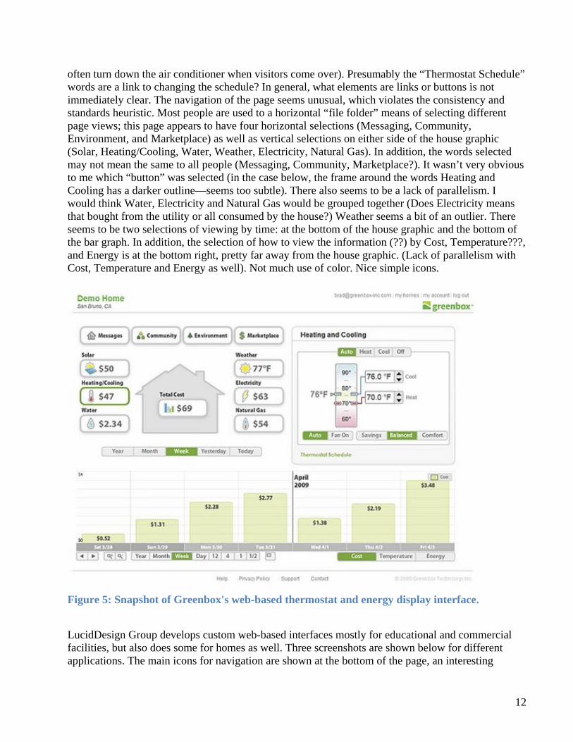
12

often turn down the air conditioner when visitors come over). Presumably the “Thermostat Schedule” words are a link to changing the schedule? In general, what elements are links or buttons is not immediately clear. The navigation of the page seems unusual, which violates the consistency and standards heuristic. Most people are used to a horizontal “file folder” means of selecting different page views; this page appears to have four horizontal selections (Messaging, Community, Environment, and Marketplace) as well as vertical selections on either side of the house graphic (Solar, Heating/Cooling, Water, Weather, Electricity, Natural Gas). In addition, the words selected may not mean the same to all people (Messaging, Community, Marketplace?). It wasn’t very obvious to me which “button” was selected (in the case below, the frame around the words Heating and Cooling has a darker outline—seems too subtle). There also seems to be a lack of parallelism. I would think Water, Electricity and Natural Gas would be grouped together (Does Electricity means that bought from the utility or all consumed by the house?) Weather seems a bit of an outlier. There seems to be two selections of viewing by time: at the bottom of the house graphic and the bottom of the bar graph. In addition, the selection of how to view the information (??) by Cost, Temperature???, and Energy is at the bottom right, pretty far away from the house graphic. (Lack of parallelism with Cost, Temperature and Energy as well). Not much use of color. Nice simple icons.

Figure 5: Snapshot of Greenbox's web-based thermostat and energy display interface.

LucidDesign Group develops custom web-based interfaces mostly for educational and commercial facilities, but also does some for homes as well. Three screenshots are shown below for different applications. The main icons for navigation are shown at the bottom of the page, an interesting

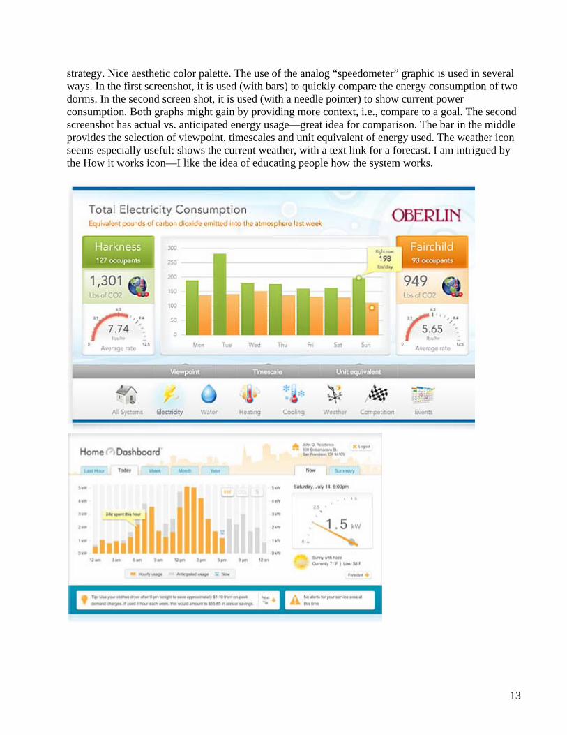
13

strategy. Nice aesthetic color palette. The use of the analog “speedometer” graphic is used in several ways. In the first screenshot, it is used (with bars) to quickly compare the energy consumption of two dorms. In the second screen shot, it is used (with a needle pointer) to show current power consumption. Both graphs might gain by providing more context, i.e., compare to a goal. The second screenshot has actual vs. anticipated energy usage—great idea for comparison. The bar in the middle provides the selection of viewpoint, timescales and unit equivalent of energy used. The weather icon seems especially useful: shows the current weather, with a text link for a forecast. I am intrigued by the How it works icon—I like the idea of educating people how the system works.

14

Figure 6: Three screenshots from Lucid Design Group's web-based interfaces.

In summary, the types of information typically available through in home displays include: Typical displays for in-home energy displays include:

Household energy use (whole house energy consumption, use by appliance) o Internal data

instantaneous power (watts) current energy consumption (in dollars per hour or kilowatt per hour) cumulative electricity consumed (kilowatt-hours), (for current day or since

installation) graphic of consumption (spinning disk to emulate energy consumption)

o Internal comparisons energy consumption/budget compared to user-set goal compare current energy consumption with a similar day (based on high and

low temperatures, solar irradiance) compare current energy consumption to similar day/month last year

o External comparisons Energy consumption comparison to neighbors/”people like me”

Cost of energy used o cumulative cost of electricity (dollars) o projected monthly bill (dollars) o comparison to established budget o current electricity rate

Energy savings equivalent to greenhouse gas or CO2 emissions avoided in pounds, trees planted, conserved gasoline, or cars taken off road

Status: the system is working within norms (e.g., space and/or water heating, appliances) Alerts (i.e., maintenance, messages) Other data

o Time/date o Temperature o Tips on what to do to save energy

15

status indicator (i.e., battery and/or wireless signal strength The web-based energy displays show some commonalities. All show weather forecast. All show some environmental effect: the first two have a page labeled Environment, Lucid calls theirs Green Features. Gridpoint shows carbon dioxide emissions averted through use of renewables; Lucid shows carbon dioxide emissions emitted from energy consumption. All provide a selection of timescales. GridPoint has a drop down menu (not the most usable since the choices are not all visible), Greenbox shows all selections at once as buttons, and Lucid Design Group uses a file folder type display. None of them have very obvious Help buttons. This section has provided an evaluation of several in-home energy displays, both stand-alone units and web-based displays.

5.2 Residential Thermal Comfort 

5.2.1 Survey data review

The first task was to evaluate how people currently use their thermostats in their homes in order to assess potential control algorithms. I reviewed the literature, especially survey data, and teamed up with Alan Meier of LBNL to develop a thermostat user survey. I reviewed national and California state data on thermostat use, as well as a national HVAC marketing survey. The housing characteristics tables of the 2005 Residential Energy Consumption Survey (RECS) from the Energy Information Administration (Energy Information Administration (EIA) 2005) provided both US and California data. The Residential Appliance Saturation Survey (RASS) (KEMA and Tobiasson 2006) supplied data on California thermostat use and settings. The American Home Comfort Survey provided national marketing information on thermostat use (Decision Analyst 2008). We were interested in the following questions: what types of thermostats do people use? How do they use them? What features are used or not used? What do people want in a thermostat? The purpose of the review was to consider what algorithms might be developed to save energy but still be found to provide acceptable comfort by people. The survey was administered by the Center for the Built Environment at UC Berkeley and hosted by the Home Energy Savers website run by LBNL. The results noted here were from September 2010 through May 2011. There were approximately 1000 responses, from all over the United States. While this survey was not representative of the population as a whole—a bias towards the computer savvy and those interested in energy issues—the comments proved invaluable to providing insight on how people are using thermostats. The following sections describe the responses from the literature review as well as the survey conducted.

16

5.2.1.1 What types of thermostats do people use?5 For the purposes of this study, I defined three types of thermostats: programmable, setback/clock, and manual6.

Manual thermostat (could be rectangular or like the Honeywell round):

Clock setback thermostat (can automatically change the setpoint at night):

Programmable thermostat (can automatically change the setpoint at night and day): The majority of respondents (63%) reported having a programmable thermostat with 32% reporting a manual thermostat. This is NOT representative of the US as a whole (of those who have thermostats, 35% have programmable). This survey is skewed towards those who have computers (online survey) and who have an interest in saving energy in their homes (visit the home energy saver website). Compared to U.S. data: In the 2005 RECS, 14% of U.S. households report having no thermostat, 30% have a programmable thermostat (PT) (34.6% of thermostat owners), and 56% have a manual thermostat (Energy Information Administration (EIA) 2005). According to the American Home Comfort Survey, 42% of households had programmable thermostats in 2008, up from 36% in 2004 (Decision Analyst 2008)7. The 2005 RECS reports for California, 19% of households report having no thermostat, 44% have a PT (54% of thermostat owners), and 37% a manual thermostat; these numbers differ from the national probably mostly due to milder weather (for those without thermostats) and the last 30 years of energy code requiring a setback or programmable thermostat. Of those that use central air conditioning in California, 68% have programmable thermostats; this most likely reflects the fact that homes built in the past 30 years are more likely to have central air conditioning.

5.2.1.2 How are thermostats used? In this survey, 60% use the off switch during the cooling season, one third on a daily basis. By contrast, 47% use the off switch during the heating season. What is difference between heating your house and cooling it that one would use the off switch more often for cooling? Many air conditioning systems are now installed in houses in climates where they are only used several days out of the year;

5 In both RECS and RASS, the authors note problems with people understanding what a programmable

thermostat is. In RECS, the authors note that the response varied depending on how the question is asked—if asked “can you set it so that the temperature setting automatically changes at the times of the day or night that you choose?”, the households reporting a programmable thermostat nearly dropped in half compared to the previous survey. RASS also noted that the numbers listed were most likely lower than expected (e.g., the response rate for post-1995 houses was expected to be 100% due to energy code, but was underreported).

6 Definitions by others differ. Manual thermostats are often called standard or mechanical. The AHCS uses the terms programmable/setback, digital/electronic (I think this refers to the display/actuation function), and mechanical.

7 It is difficult to know why the two surveys differ; my guess is given the experience of RECS stated above in footnote 1, the AHCS may overreport programmable thermostats since the survey doesn’t appear to clarify the definition of PT.

17

thus the system might be OFF most of the season, except when needed (e.g., a combination of hot outdoor temperature and someone at home). In a California study that compared the energy consumption of manual thermostats versus programmable thermostats in CA households, PTs were set slightly higher (i.e., 0.7-1.2F) than manual thermostats, but were not in OFF mode as often in the cooling season. In the heating season, PTs were set higher than manual, and far fewer were placed in OFF mode as manual thermostats (Haiad et al. 2004).

5.2.1.3 How many of the programmable thermostats are actually programmed? Programmable thermostats can be programmed to change temperature setpoints on a schedule. However, most PTs have two options—hold and override/temp—that aborts the programmed schedule; override or temporary mode typically allows a temporary setpoint until the next scheduled setpoint change but the hold mode is a permanent change, and functionally reverts the PT into a manual thermostat. For this survey, the questions did not clearly indicate whether the thermostat programming or the household member setback or setup the temperature at night, during the day, or when someone was at home. There were more responses for “never” nighttime setup for AC (53%) than “never” nighttime setbacks for heating (27%); this makes sense given that one can wear more layers and have more blankets at night (increase clo value) to improve comfort at night in the winter. In addition, temperatures are cooler at night, so people may not have bothered changing the setting on the air conditioner because it wouldn’t run at night anyway based on the temperature. Changing clo value for the summer is limited—at some point, it is difficult to sleep when it’s too hot (above 80-82F depending on humidity levels and air speed). When asked, Why not adjust the temperature at night, 28% responded that it was more comfortable not to, 15% agreed that it took the house too long to return to comfortable temperatures, another 15% thought it was inconvenient, and another 15% felt it did not save energy. For the same question except during the day, 19% responded it was more comfortable not to and 15% agreed that it took the house too long to return to comfortable temperatures. According to RECS, during the heating season, 60% of households use PTs to reduce temperature at night and 45% to reduce temperature during the day; during the cooling season, 55% of households use PTs to increase temperature at night as well as during the day8. According to the recent RASS mentioned above, of the households that setup the temperature for air conditioning (AC) during the day, 58% had programmable thermostats. However, of the households that left the AC at a constant temperature, 57% had programmable thermostats, which suggests that the programmable thermostat is not being used to change the setpoints automatically (CEC 2004). The 2003 RASS study concluded that “the results illustrate that the presence of programmable thermostats does not appear to dramatically affect setback behaviors” (CEC 2004). Of the recent buyers of HVAC equipment, the AHCS reported that 56% of homeowners always program their thermostats, 32% sometimes

8 The RECS shows a high number of respondents who responded “unknown” when asked whether the

temperatures were set higher during the day when no one was home or at night for sleeping.

18

program9, 9% never program their thermostats, and 3% do not know how (Decision Analyst 2008). Male head of household tended to be the last one to program more than female head of household.

5.2.1.4 How many thermostats are in “hold” or “override” mode? Most of the respondents never (30%) or rarely (22%) use the hold mode, but 19% use it daily. Many (36%) responded this was because they could operate the system more effectively manually, but a full 20% indicated that the household schedule was too variable for a regular programmed schedule. Override seemed to be used more often than hold, with only 15% never and 25% rarely using this mode. The most common reason for the override was for comfort (58%) followed by temporary schedule changes (35%). Comparing this study to the literature: A study conducted by thermostat manufacturer Carrier looked at the operating mode of installed programmable thermostats in households within the jurisdiction of four utilities, LIPA, ConEd, SCE, SDG&E. Of the 35,471 thermostats monitored overall, only 47% were in Program mode in which the thermostat uses the schedule previously input by the occupant to control temperature setpoints. The rest were in Hold mode, which effectively overrides the programming features and turns the thermostat into a manual thermostat. The households within the two southern California utilities showed a higher percentage (65%) in program mode, although it is unclear why (Archacki 2003). These two studies indicate that at least a third if not half of programmable thermostats in California are not used as designed, which is to change temperature setpoints based on a schedule. In the AHCS, no distinction is made between override and hold. One questions asks about the frequency of overrides for recent HVAC buyers (all the time 8%, often 12%, Sometimes 36%, Rarely 35%, Never, 9%) (Decision Analyst 2008). It is difficult to know whether overriding “all the time” means the thermostat is in Hold mode or not.

5.2.1.5 Are the owners of programmable thermostats achieving expected energy savings? In the AHCS, 1 in 6 replacement HVAC buyers saw no change in energy costs or an increase in cost. When asked the reasons for not meeting savings expectations, 57% of replacement buyers indicated increased cost of energy, 20% overriding, 12% indicated that the thermostat was difficult to program, 9% said the PT was not programmed correctly, 8% did not know how to program, and 5% did not program the PT (Decision Analyst 2008).

5.2.1.6 Usability A few questions dealt with thermostat usability. When asked about why Hold mode was used, 7% responded because the settings are too difficult to change. Many (39%) mentioned having an easier means of programming the thermostat would be helpful while another 21% agreed that a setup wizard would be helpful. About one fifth thought larger font size would be helpful and 15% thought larger buttons would help. In the open-ended answer section, several replied that the thermostat was in a location that was difficult to reach or too dark to see. A few requested other features, such as a timer, occupancy sensor, or one-touch away and resume button. One responder suggested that instead of energy savings mode for unoccupied and nighttime, have a constant energy savings mode, and just adjust the temperature when occupied: “I have the thermostat programmed lower than we usually

9 I am not sure what is meant by “sometimes program”—perhaps this refers to using override, hold or off mode

the rest of the time??

19

find comfortable so if we go out we don't have to change it and when we are home we can just bump it up a couple of degrees.”

5.2.1.7 Comfort issues Thermal comfort is defined as “the state of mind in humans that expresses satisfaction with the surrounding environment” (American Society for Heating Refrigerating and Air-Conditioning Engineers (ASHRAE) 2004). One open ended question in the survey addressed thermal comfort issues: Please describe any other issues related to being too hot or too cold in your home. Respondents reported thermal comfort related to physical measures (e.g., house construction), certain behaviors, and especially social issues. These are described in this section. Physical parameters regarding thermal discomfort in homes included house construction (lack of insulation, leaks, older uninsulated windows, multiple levels—hotter upstairs than down, additions—different insulation levels and different HVAC equipment), equipment (older, under- or over-sized, poorly balanced), and environment (angle of sun in winter versus summer and radiative heat gain through walls and windows, wind). Example comments:

“During cold snap even though the air is at 72F the coldness of some surfaces (i.e. uncovered windows, poorly insulated walls) create discomfort where there is a need to increase temperature setpoint.” “House built 1931 has no wall insulation. Windy conditions create cool walls resulting in no radiant heat reflection to room at 68 degrees, which causes it to feel colder than the temperature indicates.”

“Due to latent load in midwest, don't use setback on AC beyond mid-June.”

Social parameters included behavioral elements, personal characteristics, and household dynamics. Behavioral elements dealt with what people did to improve their thermal comfort, such as wear different clothing.

“We dress warmly in Winter, so have no problem adjusting to the temp we set automatically. Summer we wear light clothes in the house.”

Personal characteristics included age (elderly, newborn or young children need warmer temps in winter), medical conditions, and gender differences (both PMS and menopause mentioned).

“Senior citizens- we are not comfortable at the lower settings in winter time.”

“When I was younger I kept the house at 65 during the day and 62 at night. I now find that too cold. At 65 years old I now keep the house at 68 during the day and 65 at night. I have three programmable thermostats, and 2 manual in guest bedrooms that are turned down to 52 unless someone is coming.”

“We have two very young children that sleep poorly if their rooms get too cold. For that reason we tend to keep the heat on higher at night than we would otherwise.”

20

“I have medical conditions which make my hands and feet extremely cold even in hot weather. I have difficulty being comfortable; too hot upstairs, too cold downstairs.”

“I have allergies, and sensitive to a lot of heat blowing, especially during the times we are in bed.”

Household dynamics included differences in comfort or thermostat settings between gender such as husband and wife as well as generation, adults versus teenagers.

“My husband and I vary about our degrees of comfort regarding heat or cold.” Many mentioned variability in thermal comfort (e.g., “feeling” hot or cold not strictly related to numeric temperature). Some remarked on this difference with respect to seasons; others indicated solar radiation or radiation from surfaces (walls, floor) makes a difference.

“The t-stat, any t-stat, can say 74 degrees and I may feel comfortable. A day later, or even an hour later, it may say 74 and I may feel too cold. Or too warm! What simply makes no sense to anyone is why we feel ok at say 68 in the wintertime wearing a polo shirt and jeans, but would be overwarm at 70, while in the summertime, we would be freezing at 70 and feel comfortable at 74 or 75? And t-stat sensors (most of them are co-located with the interface), whether or not they are accurate, are only point sensors and do not take into account the temp at other parts of the house. There is a lot more to comfort than the temp measured at the sensor.” “At sundown in the winter, even though the thermostat shows a constant temperature, the house feels cooler. In the summer, when I leave the house for the weekend, I turn the temperature up. When I return on a very hot day, the system struggles for a long time to bring down the temperature.” “We have a manual thermostat. It's set to 65 or something like that but sometimes it feels colder than that and the heater doesn't go on, but sometimes it feels warm enough and the heater does go on.” “I can set the thermostat at the same temperature every day and still be too warm one day (or minute!) and too cold the next day (or minute)...at the same temperature. Most times, I end up with a space heater blowing right on me to maintain a consistent temperature and turn down the furnace. That's how I am most comfortable.”

5.2.1.8 Unused and wanted thermostat functions There were two open-ended questions that asked about thermostat functionality—functions that one doesn’t use and functions that one wished one’s thermostat had but it currently doesn’t. The functions reported not used fell in four general categories: those not used because not needed (e.g., programming for those with variable schedule, emergency heat, vacation, override, Day away), because it was not applicable (e.g., humidistat, heat-cool switch), because it didn’t work well, and because the user did not know how to use it (e.g., Energy saver switch).

Yes, vacation settings and such. When we are away for extended periods, we just select an appropriate temperature and set it to "hold."

21

I never use the override, and since my wife and I are home all day, I have not used the morning leave and evening return function.

Although my thermostat is programmable I keep it in the manual mode. My schedule is variable and I need the flexibility.

Yes. Instead of programming the time you want the furnace to come on in the morning, you can program the time you want the house to reach the set temperature, and the thermostat decides when to turn on the furnace. This feature didn't work well, so I don't use it any more. Energy function, do not know how it works. If I did then I would make better use.

The respondents were quite creative with respect to desired functions, such as drifting temperature setpoint at night, using outdoor temperature especially the previous day’s peak or lowest temperature, using outdoor humidity sensor, seeing indoor temperature trend and cycle rate of equipment, dynamic temperature setpoint based on a difference in temperature rather than static setpoint, control windows and whole house fan appropriately, timer, and simple seasonal occupied versus not-occupied/sleeping buttons.

Probably another set back at night in the summer. You tend to be hot when you go to bed, but as body temp cools it would be great to bring the temp up a degree or 2 to save energy. Temperature also controlled by outside temperature vs the day befores temperature, or an average thereof. Some way to report what the temperature has been and what fraction of the day/night the heat or AC has needed to be on. This would help us adjust the programming to better save energy. I want the ability to control a variable temperature range that will cause the furnace to turn on, for example; if the temp in the home rises/falls more than X degrees, the furnace will turn on. had an outside sensor to adjust the indoor temp. based on the temp. and humidity levels outside. It was tied to the external weather conditions. I leave my windows open for a good part of the year; it would be great if there was a monitoring system that would raise and lower my windows based on the outside temperature, and that would turn on the whole house fan rather than use the AC when appropriate. I would love to set the thermostat to 62 and then if anyone needs to warm it to 68 or 70, always set it back automatically after 15 or 20 minutes. My work schedule varies Mon-Fri., go to work anywhere between 7:30 a.m. and 2 p.m., return home at 5:30 or 6:30 p.m. Impractical to have a thermostat with a set daily schedule. I need 4 programmable buttons: Winter Cooler (65, for sleeping and

22

unoccupied home), Winter Warmer (74, home occupied and awake), Summer Cooler (80, sleeping), Summer Warmer (82, awake). When I arrive home from work or go to bed, punch the appropriate button. It could tell me what setting I need to keep my pipes from freezing, OR it could keep track of outside and wall temps and automatically compensate and keep the pipes from freezing.

5.2.1.9 What temperature settings do people use? For the cooling season in California, 22% of households indicate use of their central air conditioning system all the time, 24% quite a bit, 45% only a few times when needed, and 7% not at all (Energy Information Administration (EIA) 2005)10. The following graph shows the distribution of temperature settings during the cooling season. There is a clear trend of lower temperatures during the day when someone is at home versus when someone is away. Nighttime temperature show a much wider range. It is surprising to see so many households using such low temperatures for cooling (70-73F).

Figure 7: Thermostat setpoints for air conditioning in California households.

With respect to heating setpoints, the temperatures are certainly lower when no one is at home and at night, as seen in the figure below.

10 Note that more than half of households (53% during heating season and 57% during cooling season) report that someone is at home all day.

23

Figure 8: Thermostat setpoints for heating in California households.

An initial analysis of the RASS database of thermostat settings indicated that outdoor temperatures influence indoor temperature settings. The figure below compares temperature setpoints in the Imperial Valley (climate zone 15) in southeastern California with those in the Central Valley (climate zones 9, 10, 11, 13). The daily maximum summer temperatures average 108F in Imperial Valley and 93F in the Central Valley. Note that more households use higher setpoints in Imperial Valley than in the Central Valley.

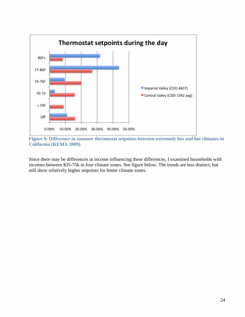
24

Figure 9: Difference in summer thermostat setpoints between extremely hot and hot climates in California (KEMA 2009).

Since there may be differences in income influencing these differences, I examined households with incomes between $35-75k in four climate zones. See figure below. The trends are less distinct, but still show relatively higher setpoints for hotter climate zones.

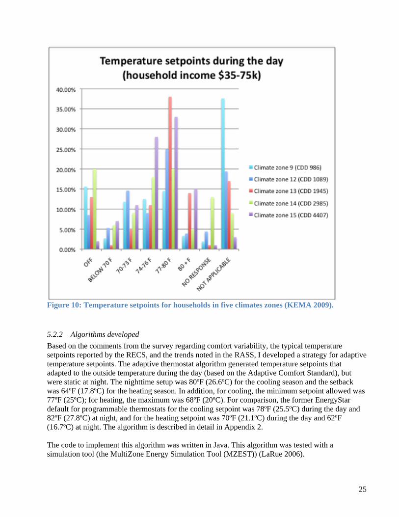
25

Figure 10: Temperature setpoints for households in five climates zones (KEMA 2009).

5.2.2 Algorithms developed

Based on the comments from the survey regarding comfort variability, the typical temperature setpoints reported by the RECS, and the trends noted in the RASS, I developed a strategy for adaptive temperature setpoints. The adaptive thermostat algorithm generated temperature setpoints that adapted to the outside temperature during the day (based on the Adaptive Comfort Standard), but were static at night. The nighttime setup was 80ºF (26.6ºC) for the cooling season and the setback was 64ºF (17.8ºC) for the heating season. In addition, for cooling, the minimum setpoint allowed was 77ºF (25ºC); for heating, the maximum was 68ºF (20ºC). For comparison, the former EnergyStar default for programmable thermostats for the cooling setpoint was 78ºF (25.5ºC) during the day and 82ºF (27.8ºC) at night, and for the heating setpoint was 70ºF (21.1ºC) during the day and 62ºF (16.7ºC) at night. The algorithm is described in detail in Appendix 2. The code to implement this algorithm was written in Java. This algorithm was tested with a simulation tool (the MultiZone Energy Simulation Tool (MZEST)) (LaRue 2006).

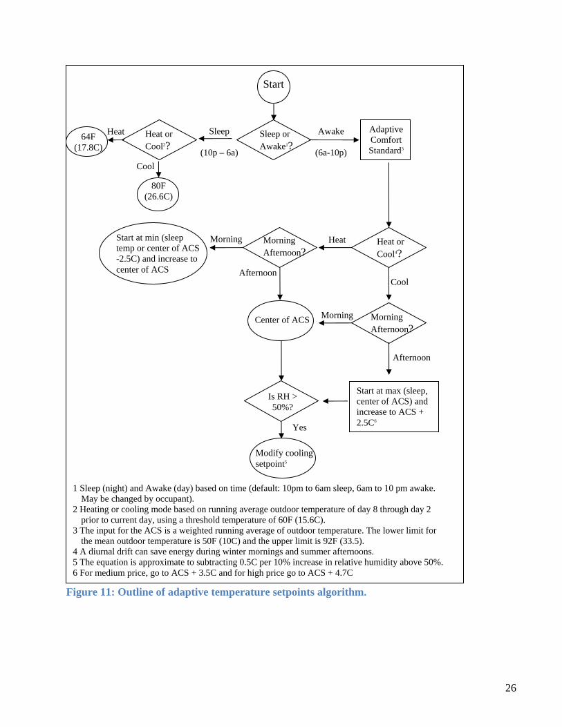
26

Figure 11: Outline of adaptive temperature setpoints algorithm.

Start

Sleep or Awake1?

Heat or Cool2?

80F (26.6C)

Cool

Heat Sleep

(10p – 6a)

Awake

(6a-10p)

Adaptive Comfort Standard3

Heat or Cool4?

HeatMorning Afternoon?

Morning Afternoon?

MorningCenter of ACS

Cool

MorningStart at min (sleep temp or center of ACS -2.5C) and increase to center of ACS

Start at max (sleep, center of ACS) and increase to ACS + 2.5C6

Afternoon

Afternoon

Is RH > 50%?

Yes

Modify cooling setpoint5

64F (17.8C)

1 Sleep (night) and Awake (day) based on time (default: 10pm to 6am sleep, 6am to 10 pm awake. May be changed by occupant).

2 Heating or cooling mode based on running average outdoor temperature of day 8 through day 2 prior to current day, using a threshold temperature of 60F (15.6C).

3 The input for the ACS is a weighted running average of outdoor temperature. The lower limit for the mean outdoor temperature is 50F (10C) and the upper limit is 92F (33.5).

4 A diurnal drift can save energy during winter mornings and summer afternoons. 5 The equation is approximate to subtracting 0.5C per 10% increase in relative humidity above 50%. 6 For medium price, go to ACS + 3.5C and for high price go to ACS + 4.7C

27

5.2.3 Tests

I ran the simulation using a validated house model with MZEST to test the residential adaptive comfort temperature setpoints. The simulation compared the heating and cooling energy used for a house using the adaptive temperature setpoints and one using EnergyStar default setpoints for a programmable thermostat for an entire year. It used Sacramento, California temperature data.

5.2.3.1 Annual simulation The first step was to compare an annual simulation of the adaptive temperature setpoints to energy-saving default setpoints from an EnergyStar programmable thermostat. The adaptive temperature setpoints for heating and cooling were based on the method outlined in the appendix for 90% acceptability. The following graph shows the indoor temperature for both simulations as well as the running weighted average outdoor temperature for an entire year. Note the increase in setpoint in the summer months for the adaptive setpoints compared to the static setpoints. The peak indoor temperature is 29ºC (84.2ºF) when the weighted average outdoor temperature reaches 25ºC (77ºF).

Figure 12: Annual simulation indoor temperatures.

An initial look at the data suggested a few problems. For one, the diurnal change of the adaptive setpoints caused the air conditioner to run more often in the evening. In addition, sometimes the air conditioning was on in the fall and spring afternoons when the outdoor temp was lower than the indoor temperature. According to several studies, air conditioner use in these circumstances does not reflect real world conditions.

Indoor Temperature for Adaptive vs. Programmable Thermostat

0

5

10

15

20

25

30

35

Time (1 year in 1 hour increments)

Tem

pera

ture

C

32

42

52

62

72

82

92

AT-Temp PT-Temp Outdoor Weighted Avg Temp

28

A review of the comfort votes revealed quite a number of issues. For example, of the hours that the index indicated too hot, 96% of the time the outdoor temperature was at least 3ºF (1.6ºC) cooler than the inside. Figure 12 above shows high indoor temperatures especially in the spring months, possibly a combination of the heating system and the area of west facing windows in this particular house model picking up heat gain from the low springtime sun angle. People would most likely open up windows to increase comfort for these times rather than turn on the air conditioning. Providing advice to encourage the opening of windows and outdoor temperature information would be helpful to save energy. Of the hours where the index indicated “too cold”, 93% of the time this occurred in the cooling months! Nearly a third of the time the outdoor temperature was warmer than the indoor temperature, and thus again, advice to encourage opening up the house could save energy. Two-thirds of the time, the indoor temperature was at least 64.4ºF (18ºC). The diurnal drift seemed to save energy for heating, but had less effect on summer cooling savings. Most likely the setpoint drift paralleled the indoor temperature increase due to the outdoor temperature. The effect of the drift for comfort for the cooling season is still a viable concept, but should be further tested with field research rather than simulations. The decision to switch from heating to cooling mode was based on a simple average of the previous week’s outdoor temperature, based on the Alternative Calculation Method for developing Title-24-based compliance software (California Energy Commission (CEC) 2001). However, the above temperature graphs indicate some problems with this approach, especially during the swing months of spring and fall. In general, a better understanding of behavior during the swing months would improve the performance. For example, one study by Kempton showed that people tended to withstand a greater temperature swing in the fall and spring seasons (Kempton and Krabacher 1987). Rather than switching from heating to cooling (or the reverse) in a single day, people may delay turning on the air conditioner or heater until the season develops a pattern. Although the Adaptive Comfort Standard suggests a range of comfort, the low limit for cooling seems to be too high. Some evidence indicates that during the cooling season, people do not mind being “too cold”. For example, the outdoor temperature may reach 92ºF (35ºC) in Sacramento during the day and down to 58ºF (14ºC) at night. While 68ºF (20ºC) might be found too cool according to the model, Hackett’s interviews with Davis residents found that temperatures in the 60sºF were comfortable, even refreshing especially if they expected the day to get quite warm (Hackett and McBride 2001). Given that the low limit for the Adaptive Comfort Standard for cooling may be too high especially during the swing or transition months, I then modified the comfort index slightly. For example, for days when the weather was expected to be hot, cool temperatures in the morning (i.e., > 68ºF (20ºC)) were considered comfortable on a summer morning. This was also based on the assumption that people will dress warmly for cool mornings; according to Comfort 1.07, a person with a Clo value of 1.2 is comfortable at 68ºF (20ºC). Morning temperatures between 66.2ºF (19ºC) and 68ºF (20ºC) were considered slightly cool, and below 64.4ºF (18ºC) uncomfortably cool.

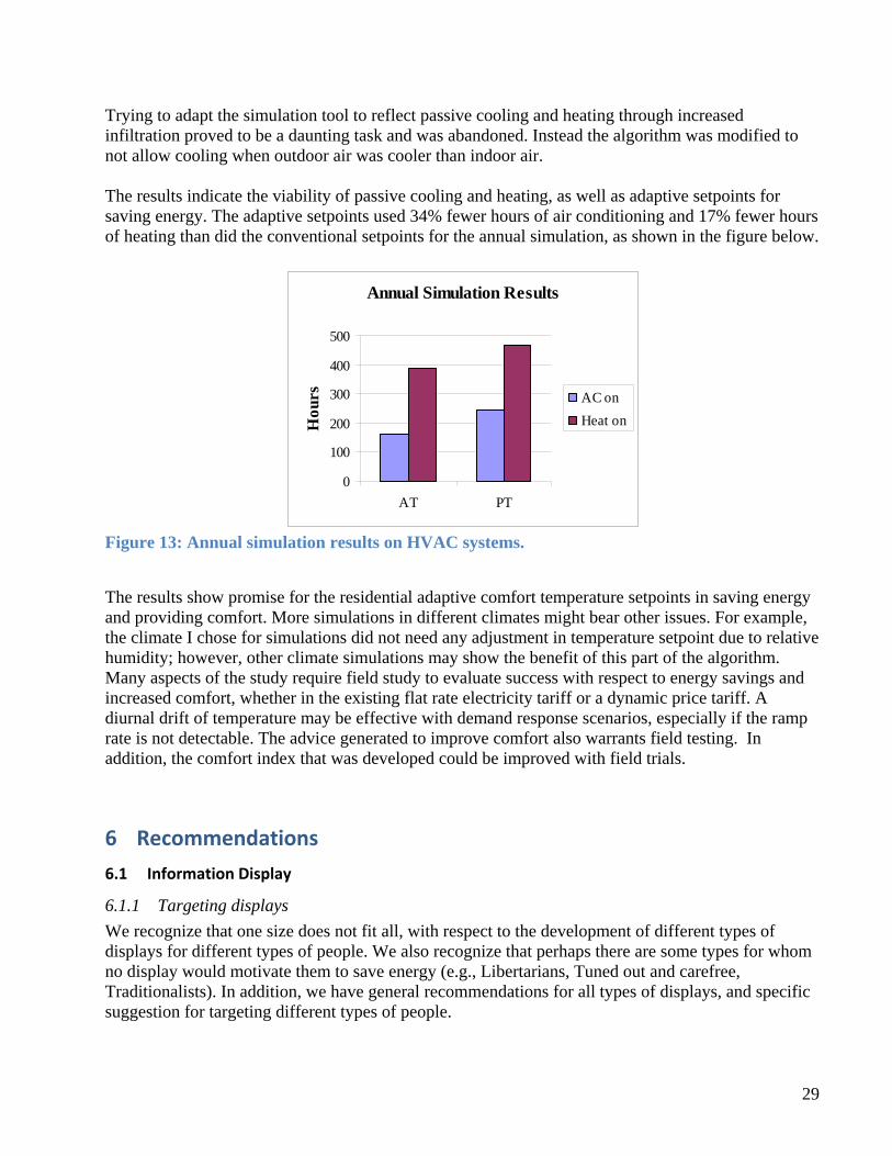
29

Trying to adapt the simulation tool to reflect passive cooling and heating through increased infiltration proved to be a daunting task and was abandoned. Instead the algorithm was modified to not allow cooling when outdoor air was cooler than indoor air. The results indicate the viability of passive cooling and heating, as well as adaptive setpoints for saving energy. The adaptive setpoints used 34% fewer hours of air conditioning and 17% fewer hours of heating than did the conventional setpoints for the annual simulation, as shown in the figure below.

Figure 13: Annual simulation results on HVAC systems.

The results show promise for the residential adaptive comfort temperature setpoints in saving energy and providing comfort. More simulations in different climates might bear other issues. For example, the climate I chose for simulations did not need any adjustment in temperature setpoint due to relative humidity; however, other climate simulations may show the benefit of this part of the algorithm. Many aspects of the study require field study to evaluate success with respect to energy savings and increased comfort, whether in the existing flat rate electricity tariff or a dynamic price tariff. A diurnal drift of temperature may be effective with demand response scenarios, especially if the ramp rate is not detectable. The advice generated to improve comfort also warrants field testing. In addition, the comfort index that was developed could be improved with field trials.

6 Recommendations 

6.1 Information Display 

6.1.1 Targeting displays

We recognize that one size does not fit all, with respect to the development of different types of displays for different types of people. We also recognize that perhaps there are some types for whom no display would motivate them to save energy (e.g., Libertarians, Tuned out and carefree, Traditionalists). In addition, we have general recommendations for all types of displays, and specific suggestion for targeting different types of people.

Annual Simulation Results

0

100

200

300

400

500

AT PT

Hou

rs AC onHeat on

30

In general, the display should be usable and engaging. This means following Nielsen’s suggestions for usability (simple to use, easy to learn and remember, aesthetically pleasing, few errors) and perhaps looking “cool”—NEST thermostat or iPhone-like. In addition, providing a means of setting goals falls into the general category. Providing specific and simple actionable tips is also recommended for the general audience. The type of display might overlap an existing use, such as computer web browser display, smart phone app, or icon on television screen. Some consideration might be taken for those who are not computer/technologically savvy; a simple interface would suffice. Three specific, targeted displays suggested are the following”

One type might focus on the economics: the cost of energy (for current day or since installation, include the embedded energy of grid energy (i.e., transmission losses)), especially the loss of money if no action is taken. This type of display might be number-centric, providing many different means of analysis, trending of days, and allow comparison of current performance with a similar day (based on high and low temps and solar irradiance) or compare similar day/month last year, Total Energy Use compared to this time last year, Household Energy Use, both whole house energy consumption and use by appliance

Another type might focus on the environment: emphasize social responsibility to reduce carbon emissions, providing energy savings equivalent to CO2 emissions avoided in pounds (this changes with location and season—depends on local utility), trees planted, conserved gasoline, averted ice melting, or cars taken off road. This type of display could be more graphic in nature, such as trees sprouting leaves when the system detects energy savings.

A third type might emphasize social issues: comparison to others’ carbon footprint, like-neighbors energy consumption. A means of using Facebook, Twitter, or other social media should be accommodated for contests, bragging rights, and in general sharing of energy consumption information and motivation. The display should be engaging and a status symbol to be used by the consumer for “bragging rights” to their friends and family that come over.

This system needs to overcome barriers of existing in-home energy displays to encourage energy saving behaviors. The in home energy display should therefore:

engage people o aesthetically pleasing, o well-composed visually o use a hierarchy of info display based on what used most often

capitalize on what is familiar o Honeywell Round thermostat o typical switches and lexicon of energy displays/computers

test new words for customer understanding o typical website navigation

31

be easy to program, memorable and simple o use Wizards and defaults o items should be grouped together in a systematic and intuitive way

use graphic display when a quick survey is needed, numeric display when more precision needed (both in some cases)

o pie charts for types of energy used inform people (provide tips to increase savings) provide comparisons display relevant information to user (i.e., allow choice in types of displays) provide feedback on actions taken feature help and error messages, alerts, notice of radio signal strength

6.2 Thermal Comfort 

Many people recognize that thermal comfort changes over the course of the year. The indoor temperatures found comfortable in the summer (68-70F) would be quite cold in the summer, due to human physiological changes, clothing levels, and other elements related to the outdoor air temperature. Improving thermal comfort with thermostat algorithms that provide setpoints that adapt to outdoor air temperature shows promise of providing the seasonal and daily variability that survey responders recognized—and save energy and money in the process. The algorithm could be improved in many ways, not the least would be to test in the field. While this algorithm considered daily and weekly changes in outdoor temperature, another improvement would be to consider the longer physiological and psychological changes with seasons. In addition, one might include these expectations in the algorithm; for example, people typically do not turn on the air conditioner during winter or the heater during summer. One improvement to the algorithm would be to recognize the variability in outdoor temperature in the spring and fall months and allow wider temperature ranges. Another enhancement would be passive heating or cooling; the thermostat could alert the occupant to open windows or turn on fans/whole house fan appropriately to allow cooling or heating the house with outdoor air. Yet another development would be to modify the temperature setpoint in anticipation of the forecasted peak temperature or low temperature. In addition, we recognize that there are many issues that influence thermal comfort and how residents operate their thermostats. Other functions such as timers and occupancy sensors can help occupants maintain comfort with variable schedules. More engaging and usable thermostat interfaces and the use of existing platforms (e.g., smart phones, computers) to program and control thermostats may also help provide better comfort.

32

7 References  American Society for Heating Refrigerating and Air-Conditioning Engineers (ASHRAE). 2004.

Standard 55-2004: Thermal Environmental Conditions for Human Occupancy. Atlanta: American Society of Heating, Refrigerating and Air-Conditioning Engineers, Inc.

———. 2005. ASHRAE Fundamentals Handbook. Atlanta: American Society of Heating, Refrigerating and Air-Conditioning Engineers, Inc.

Archacki, Raymond. 2003. Carrier Thermostat Mode Summary: Summer 2003. Arens, Edward, Stephen Turner, Hui Zhang, and Gwelen Paliaga. 2009. A Standard for Elevated Air

Speed in Neutral and Warm Environments. ASHRAE Journal. Arens, Edward, Tengfang Xu, Katsuhiro Miura, Hui Zhang, Marc Fountain, and Fred Bauman. 1998.

A study of occupant cooling by personally controlled air movement. Energy and Buildings 27:45-59.

ASHRAE. 2004. Standard 55-2004: Thermal Environmental Conditions for Human Occupancy. Atlanta, GA: American Society of Heating, Refrigeration, and Air-conditioning Engineers.

Aynsley, Richard. 2006. Cooling effect of elevated air speed. In Proceedings of the 2006 ASHRAE Annual Meeting. Atlanta: American Society for Heating, Refrigerating, and Air-Conditioning Engineers.

California Energy Commission (CEC). 2001. Residential Alternative Calculation Method (ACM) Approval Manual. Sacramento: California Energy Commission.

———. 2004. California Statewide Residential Appliance Saturation Study. Sacramento: California Energy Commission.

CEC. California Statewide Residential Appliance Saturation Study 2004. Available from http://www.energy.ca.gov/reports/400-04-009/2004-08-17_400-04-009VOL2B.PDF.

Cooper, Gail. 1998. Air Conditioning America: Engineers and the Controlled Environment, 1900-1960. Baltimore: John Hopkins University Press.

de Dear, R. J., and G. S. Brager. 1998. Developing an Adaptive Model of Thermal Comfort and Preference. ASHRAE Transactions 104 (1a):145-167.

Decision Analyst. 2008. 2008 American Home Comfort Survey. Arlington: Decision Analyst. Ehrhardt-Martinez, Karen, Kat A. Donnelly, and John A. "Skip" Laitner. Advanced Metering

Initiatives and Residential Feedback Programs: A Meta-Review for Household Electricity-Saving Opportunities 2010 [cited Research Report E105. Available from http://www.aceee.org/research-report/e105.

Energy Information Administration (EIA). 2009. Residential Energy Consumption Survey: Preliminary Housing Characteristics Tables. Energy Information Administration 20052009]. Available from http://www.eia.doe.gov/emeu/recs/recs2005/hc2005_tables/detailed_tables2005.html.

EPA. 2008. Energy Star Program Requirements for Programmable Thermostats: Eligibility Criteria (v. 1.2)2008]. Available from http://www.energystar.gov/ia/partners/product_specs/eligibility/thermostats_elig.pdf.

Foster, Ben, and Susan Mazur-Stommen. 2012. Results from Recent Real-Time Feedback Studies, Report No. B122. Washington, DC: American Council for an Energy Efficient Economy.

Fountain, Mark, and Charlie Huizenga. 1996. A Thermal Comfort Prediction Tool. ASHRAE Journal 38 (9).

33

Gruber, Angelika, and Corp. Author: Tefen. Trend-setting market segmentation- a new wave in the German energy market. Tefen 2008 [cited Oct. 12, 2009. Available from http://www.articlealley.com/article_728792_15.html.

Hackett, Bruce, and Robert McBride. 2001. Human Comfort Field Studies. Sacramento: California Energy Commission.

Haiad, Carlos, John Peterson, Paul Reeves, and John Hirsch. 2004. Programmable Thermostats Installed into Residential Buildings: Predicting Energy Savings Using Occupant Behavior & Simulation. Southern California Edison.

Herter, Karen. 2006. Effects of Critical Peak Pricing on Residential Electricity Use in California. Dissertation, Energy and Resources Group, UC Berkeley, Berkeley.

Comfort (UC Berkeley Thermal Comfort Program) 1.07 (computer software). UC Berkeley, Berkeley.

Humphreys, M. A., and J. Fergus Nicol. 1998. Understanding the Adaptive Approach to Thermal Comfort. ASHRAE transactions: Symposia 104 (1b):991-1004.

KEMA. Saturation Tables, California Statewide Residential Appliance Saturation Study (RASS) 2009. Available from http://websafe.kemainc.com/RASS2009/Query.aspx?QType=1&tabid=1.

KEMA, and Wendy Tobiasson. 2006. California Statewide Residential Saturation Study Update to Air-Conditioning Unit Consumption Estimates Using 2004 Billing Data. Sacramento: California Energy Commission.

Kempton, Willett, and Shirlee Krabacher. 1987. Thermostat Management: Intensive Interviewing Used to Interpret Instrumentation Data. In Energy Efficiency: Perspectives on Individual Behavior, edited by W. Kempton and M. Neiman. Berkeley: American Council for an Energy-Efficient Economy.

LaRue, Anna May. 2006. Distributed Sensing and Controlling of Residential HVAC Systems for Thermal Comfort, Demand Response, and Reduced Annual Energy Consumption

Masters Thesis, University of California, Berkeley, Berkeley. Loeb, Lorie. TellEmotion 2009 [cited January 13, 2009. Available from

http://www.tellemotion.com/. Lovins, Amory. 1992. Air Conditioning Comfort: Behavioral and Cultural Issues. Boulder, CO:

ESource. Lutzenhiser, Loren. 1993. Social and behavioral aspects of energy use. Annual Review of Energy and

Environment (18):247-289. ———. 1993. Social and behavioral aspects of energy use. Annual Review of Energy and

Environment 18:247-289. ———. 2009. Behavioral Assumptions Underlying California Residential Sector Energy Efficiency

Programs. Oakland: California Institute for Energy and Environment. Morgan, Craig, and R. J. de Dear. 2003. Weather, clothing, and thermal adaptation to indoor climate.

Climate Research 24:267-284. Muzer, A, J.-P. Libert, and V Candas. 1984. Ambient Temperature and Human Sleep. Cellular and

Molecular Life Sciences 40 (5):425-429. Nicol, J. Fergus, and M. A. Humphreys. 2009. The derivation of the equations for thermal comfort in

free-running buildings in European Standard EN15251. Buildings and Environment. Nielsen, Jakob. 1993. Usability Engineering. San Francisco: Morgan Kaufmann. ———. 1994b. Heuristic evaluation. In Usability Inspection Methods, edited by J. Nielsen and R. L.

Mack. New York: John Wiley & Sons.

34

Nolan, J.M., P.W. Schultz, Robert B. Cialdini, N. J. Goldstein, and V. Griskevicius. under review. Normative social influence is underdetected. Personality and Social Psychology Bulletin.

Olsen, Erik. Smart Meters Open Market for Smart Apps [Blog] 2008. Available from http://greeninc.blogs.nytimes.com/2008/10/07/smart-meters-open-market-for-smart-apps/.

Pedersen, Marc. 2008. Segmenting Residential Customers: Energy and Conservation Behaviors. Proceedings of the 2008 ACEEE Summer Study on Energy Efficiency in Buildings 7:229-241.

Peffer, Therese, Marco Pritoni, Alan K Meier, Cecilia Aragon, and Daniel Perry. 2011. How People Use Thermostats: A Review. Building and Environment 46 (12):2529-2541.

Rogers, Everett M. 2003. Diffusion of Innovations. 5th ed. New York: Free Press. Schmidt-Kessen, W, and K Kendel. 1973. The influence of room temperature on night sleep in man.

Research in Experimental Medicine 160 (3):220-233. Schultz, P.W., J.M. Nolan, Robert B. Cialdini, N. J. Goldstein, and V. Griskevicius. 2007. The

Constructive, Destructive and Reconstructive Power of Social Norms. Psychological Science 18:429-433.

Stein, Benjamin, and John S. Reynolds. 1992. Mechanical and Electrical Equipment for Buildings. New York: John Wiley & Sons, Inc.

Stein, Lynn Fryer. 2004. Final Report—California Information Display Pilot Technology Assessment. Boulder: Primen Inc.

Stein, Lynn Fryer, and Nadav Enbar. 2006. Direct Energy Feedback Technology Assessment for Southern California Edison Company. Boulder: EPRI Solutions.

Tsuzuki, Kazuyo, Kazue Okamoto-Mizuno, Koh Mizuno, and Tatsuya Iwaki. 2005. Effects of air flow on sleep stages and body temperature of humans during exposure to humid heat. Paper read at Third International Conference on Human-Environment Systems, at Tokyo, Japan.

U.S. Census Bureau. 2000 Census Data 2000. Ubbelohde, M. Susan, George Loisos, and Robert McBride. 2003. Advanced Comfort Criteria &

Annotated Bibliography on Adapted Comfort. Sacramento: California Energy Commission. Van Elburg, Henk. 2008. Smart Metering and Consumer Feedback: What Works and What Doesn't.

Proceedings of the 2008 ACEEE Summer Study on Energy Efficiency in Buildings 2:349-360. Woods, James. 2006. Fiddling with Thermostats: Energy Implications of Heating and Cooling Set

Point Behavior. Proceedings of the 2006 ACEEE Summer Study on Energy Efficiency in Buildings.

———. 2006. Fiddling with Thermostats: Energy Implications of Heating and Cooling Set Point Behavior. Paper read at ACEEE Summer Study on Energy Efficiency in Buildings, at Asilomar, CA.

Zhang, Hui. 2003. Local Thermal Comfort in Asymmetrical and Transient Environments. Doctoral Dissertation, Architecture, UC Berkeley.

35

8 Appendix 1:  List of Acronyms ACS: Adaptive Comfort Standard ASHRAE: American Society of Heating, Refrigerating and Air-Conditioning Engineers DR: Demand Response HVAC: Heating, Ventilation, and Air Conditioning LOV: List of Values MZEST: MultiZone Energy Simulation Tool PCT: Programmable Communicating Thermostat PT: Programmable Thermostat VALS: Values, Attitudes, and Lifestyles

36

9 Appendix 2: Developing the Adaptive Thermostat Algorithm  This section outlines the development of dynamic temperature setpoints suitable for residential thermal comfort, building on the Adaptive Comfort Standard by adding the effects of diurnal temperature changes, relative humidity, air movement, and suggesting setpoints for nighttime comfort. The purposes of developing a thermostat that adapts the temperature setpoints based on outside air temperature, relative humidity, and air movement are two-fold: to save energy and provide better comfort during high price periods.

9.1.1 Developing the algorithm

The objective was to use what is known about thermal comfort in residences to develop an algorithm that provides comfort, saves energy, and engages the person, not only in his/her comfort but also understanding its implications on energy use. The method described to develop the algorithm began by using the outdoor temperature, similar to the Adaptive Comfort Standard. The next step was to modify the setpoint based on time of day. Next, I modified the setpoint using relative humidity in developing a setpoint that reflects a “feels like” temperature, similar to wind chill. An additional step was to develop advice based on what the person can do to feel more comfortable, regarding opening windows and using fans to increase comfort for less cost. This section describes these steps in detail. 1) Develop a seasonal change in setpoints by using a running weekly weighted average outdoor dry bulb temperature as input to the Adaptive Comfort Standard to predict an indoor comfortable temperature range during waking hours.11 2) Develop a diurnal change in setpoint for winter mornings and summer afternoons. In the cooling months, allow the temperature to drift from the center of the comfort range to the upper limit. In the heating months, allow the temperature to drift from the lower limit of the range to the center of the range. 3) Modify the cooling setpoint based on relative humidity, since a high relative humidity reduces thermal comfort.

9.1.1.1 Develop a seasonal change in setpoint 

The Adaptive Comfort Standard provides a means for establishing a comfortable indoor temperature range for naturally ventilated buildings based on the mean monthly outdoor air temperature. As seen in the figure below, one enters a mean monthly air temperature on the horizontal axis to determine a temperature range found acceptable by 90% of the population and a range found acceptable by 80% of the population. This standard was developed using comfort votes from commercial buildings, and therefore is meant to give comfort criterion during the daytime hours. A given mean monthly outdoor temperature provides a range of operative temperatures, which could define a heating and cooling setpoint. For air velocities less than 80 fpm (0.41 m/s) and mean radiant temperatures less than 120ºF (48.9ºC), the operative temperature is approximately equal to the adjusted dry-bulb temperature,

11 Temperatures for nighttime came from laboratory sleep studies.

37

which is the average of the air and mean radiant temperatures. Thus, we will assume the operative temperature is equivalent to dry bulb temperature setpoint for the HVAC equipment.

Figure 14: The Adaptive Comfort Standard from ASHRAE 55-2004 for naturally ventilated buildings (American Society for Heating Refrigerating and Air-Conditioning Engineers (ASHRAE) 2004).

The figure below shows an example of generating heating and cooling setpoints based on the monthly outdoor temperature, using the mean monthly outside temperature from Sacramento, California. The default setpoints suggested for EnergyStar thermostats (for houses occupied during the daytime) are shown for comparison: 70ºF (21ºC) heat, 78ºF (25.6ºC) cool. The cooling setpoints for the adaptive strategy are higher than the static cooling setpoint (and the reverse for the heating setpoints). For example, in July and August when the outside temperature reaches 100ºF (37.8ºC), the adaptive thermostat temperature setpoint might drift to 82ºF (27.8ºC), which is higher than the programmable thermostat setpoint of 78ºF (25.6ºC). This represents energy savings, since the heating and cooling equipment would not cycle as often.

38

Figure 15: Adaptive temperature setpoints for a house in Sacramento, CA.

Humphreys has suggested that instead of using a monthly outdoor temperature mean, that the previous two weeks or even a week can be indicative of the adaptive effect (Humphreys and Nicol 1998). For this algorithm, I used the weighted running average of the previous seven days.12 The weighted average comes from Morgan & de Dear (2003), who developed a formula for the exponential decay of the effect of outdoor temperature on indoor clothing decisions.

“These weighting coefficients can be used to calculate the appropriate mean outdoor temperature (Tmot) for subsequent input to an adaptive indoor temperature algorithm: Tmot = 0.34TDayx-1 + 0.23TDayx-2 + 0.16TDayx-3 + 0.11TDayx-4 + 0.08TDayx-5 + 0.05TDayx-6 + 0.03TDayx-7 and then the adaptive algorithm for indoor comfort temperatures in a naturally ventilated or free running building (de Dear & Brager 2002) can be written as comfort temperature (°C) = 0.31Tmot + 17.8 (4) and the acceptable range of temperatures is defined as the optimal comfort temperature (Eq. 4) ± 2.5°C for

12 The European adaptive comfort standard, Annex A.2 of EN15251, uses an exponentially-weighted running

mean outdoor temperature and is well described in (Nicol and Humphreys 2009).

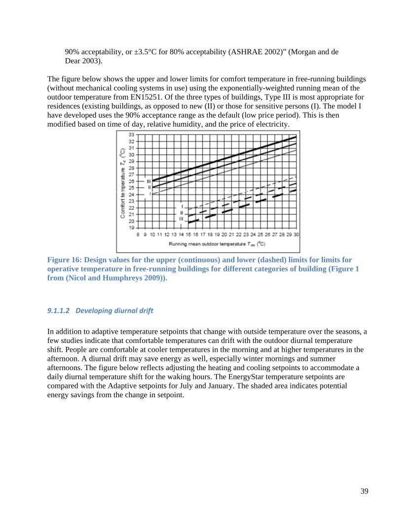
39

90% acceptability, or ±3.5°C for 80% acceptability (ASHRAE 2002)” (Morgan and de Dear 2003).

The figure below shows the upper and lower limits for comfort temperature in free-running buildings (without mechanical cooling systems in use) using the exponentially-weighted running mean of the outdoor temperature from EN15251. Of the three types of buildings, Type III is most appropriate for residences (existing buildings, as opposed to new (II) or those for sensitive persons (I). The model I have developed uses the 90% acceptance range as the default (low price period). This is then modified based on time of day, relative humidity, and the price of electricity.

Figure 16: Design values for the upper (continuous) and lower (dashed) limits for limits for operative temperature in free-running buildings for different categories of building (Figure 1 from (Nicol and Humphreys 2009)).

9.1.1.2 Developing diurnal drift 

In addition to adaptive temperature setpoints that change with outside temperature over the seasons, a few studies indicate that comfortable temperatures can drift with the outdoor diurnal temperature shift. People are comfortable at cooler temperatures in the morning and at higher temperatures in the afternoon. A diurnal drift may save energy as well, especially winter mornings and summer afternoons. The figure below reflects adjusting the heating and cooling setpoints to accommodate a daily diurnal temperature shift for the waking hours. The EnergyStar temperature setpoints are compared with the Adaptive setpoints for July and January. The shaded area indicates potential energy savings from the change in setpoint.

40

Figure 17: Changing the adaptive temperature setpoints over the course of a day.

For cooling during waking hours, the lowest temperature setpoint is based on the center of the Adaptive Comfort Standard for that month, then gradually rising +2.5ºC to peak at the maximum 90% acceptability temperature allowed by the ACS. The temperature setpoint during the day follows the outdoor temperature. For heating during waking hours, the temperature setpoint starts at the minimum 90% acceptability temperature and rises to peak at the center of the Adaptive Comfort Standard in the afternoon. During cold weather, the temperature setpoint is lower in the morning, and then remains at the peak until the person goes to sleep. The temperature setpoints were modified at night for energy savings, just like the default settings for programmable thermostats. Physiological evidence supports a nighttime winter setback for heating, but not a nighttime summer setup for cooling. Of the six factors that influence thermal comfort (air temperature, humidity, air speed, radiation, metabolic rate (Met), and clothing value (Clo)), the two personal elements of thermal comfort, Met and Clo, are conducive to winter nighttime temperature setback. Not only do people tend to have a higher insulation value (blankets, comforters) at night, but physiologically, a person’s core temperature changes approximately 0.4ºC (0.7ºF) over the course of the day, peaking in the late afternoon and at its lowest point at night (Zhang 2003). Several studies concur with thermoneutrality of 86ºF (30ºC) inside the bed, and increased wakefulness if this temperature drops below 78.8ºF (26ºC) with ambient temperature of 55.4ºF (13ºC). Preferred nighttime room temperature was found to be 66.2ºF (19ºC) (Muzer, Libert, and Candas 1984). A

Diurnal Temperature Setpoint Strategy

1011121314151617181920212223242526272829303132333435

1 2 3 4 5 6 7 8 9 10 11 12 13 14 15 16 17 18 19 20 21 22 23 24

Time of Day

Tem

pera

ture

C

50

55

60

65

70

75

80

85

90

95

Tem

pera

ture

F

AdaptCool JulAdaptHeat JanEnergyStarcoolEnergyStarheat

Sleep Wake

41

survey of 100 houses showed average winter temperatures set at 65.3-66.6ºF (Woods 2006). The EnergyStar default for nighttime setback is 62ºF; I used a static 64ºF (17.8ºC) nighttime setback from 10 pm to 6 am. But what about the summer nighttime temperature setup? On one hand, nighttime outdoor temperatures tend to drop within a comfortable temperature range for most climates in California, and the indoor temperatures tend to follow the outdoor temperatures with some time lag. Also, when a person is asleep, he or she is less aware of the temperature (personal correspondence, Zhang). But on the other hand, some climates do not cool down at night. Several studies have been conducted to determine the effect of temperature on sleep, with mixed results. Tsuzuki et al (2005) suggested if the air temperature was above 26ºC (78.8ºF) or the relative humidity was high, or person was clothed, then the person may be uncomfortable and unable to fall asleep unless adequate air flow was provided (Tsuzuki et al. 2005). Several studies show better sleep at 26-27ºC (78.8-80.6ºF) compared to 31 or 36ºC (87.8 or 96.8ºF) (Schmidt-Kessen and Kendel 1973). The Residential Appliance Saturation Survey (RASS) shows an average of 79.6ºF (26.4ºC) at night (California Energy Commission (CEC) 2004) and Woods reports 77.4 – 78.4ºF at night (Woods 2006). The EnergyStar setup for night is 82ºF (27.8ºC). Based on these studies, I chose 26.6ºC (80ºF) as a static nighttime setup from 10 pm to 6 am. In summary, the algorithm generated temperature setpoints that adapted to the outside temperature during the day, but were static at night. In addition, for cooling, the minimum setpoint allowed was 77ºF (25ºC); for heating, the maximum was 68ºF (20ºC). The nighttime setup was 80ºF (26.6ºC) for the cooling season and the setback was 64ºF (17.8ºC) for the heating season. For the programmable thermostat, the EnergyStar default for the cooling setpoint was 78ºF (25.5ºC) during the day and 82ºF (27.8ºC) at night, and for the heating setpoint was 70ºF (21.1ºC) during the day and 62ºF (16.7ºC) at night.

9.1.1.3 Modifying setpoint for high relative humidity 

The next step involves adding the effect of relative humidity on the daytime comfort setpoint using effective temperature (ET*) and discomfort index (DISC). ET*, the effective temperature, is the temperature at 50% relative humidity that yields the same total heat loss from the skin as for the actual environment (American Society for Heating Refrigerating and Air-Conditioning Engineers (ASHRAE) 2005). It can be thought of as a “feels like” temperature; high relative humidity causes the temperature to “feel” warmer, similar to the effect of wind chill causing the temperature to feel cooler. DISC provides a scale for discomfort from -4 (Intolerably cold) to +4 (Intolerably hot) as follows:

4-Intolerable 3-Very uncomfortable 2-Uncomfortable 1-Slightly uncomfortable 0-Comfortable

I used the two-node comfort model software tool, Comfort 1.07 (Fountain and Huizenga 1996; Huizenga and Fountain 1997), to generate the effective temperature curve for a given temperature at various relative humidities. The effect of relative humidity on the temperature can be seen in the

42

following figure, which plots the effective temperature and discomfort index. According to this figure, humidity level does not seem to affect comfort at low temperatures, but has an increasing effect on temperatures greater than 25ºC (77ºF). For example, 77ºF (25ºC) feels slightly warmer (77.7ºF (25.4ºC)) at 80% relative humidity, but 80.6ºF (27ºC) feels even warmer (82.2ºF (27.9ºC)) at 80% relative humidity and slightly cooler 79.9ºF (26.6ºC) at 20% relative humidity. The figure below indicates that indoor temperature setpoints greater than 79ºF (26.1ºC) should be reduced if the relative humidity is greater than 70%.

Figure 18: Effect of relative humidity on comfort.

The figure below shows a graphic summary of developing temperature setpoints. First, choose the comfort temperature predicted from the Adaptive Comfort Standard using a weighted running mean of outdoor temperature. Second, choose a comfort range, based on occupant preference. Then adjust the setpoint based on the time of day. Finally adjust the cooling setpoint based on the relative humidity.

43

Figure 19: Summary of adaptive setpoints.

9.1.2 Advice generation to engage energy saving behavior

Many behaviors can help save energy and reduce costs during high peak periods. While some people already open and close windows appropriately to save energy, others may need prompting and information to do so. Similarly, air movement with fans will provide comfort at higher temperatures. Yet some people may not know how much money can be saved by using ceiling fans instead of air conditioning. One rule of thumb used for natural ventilation of buildings is that if the outdoor temperature is at least 3ºF (1.6ºC) cooler than the inside, opening windows can cool the building (Stein and Reynolds 1992). Initially, a prompt to open the windows and/or turn on the whole house fan can be provided through the user interface; perhaps future control systems will handle the control of an economizer or whole house fan. In a similar vein, in the winter, if people are too hot, they are likely to open a window if the outdoor temperature is lower than indoor, especially if they have information about the outdoor temperature. Also, one might assume the reverse is true, that if the outdoor temperature is higher than indoor and people are too cold, they will open up a window. Another source of comfort is moving air. One study found that a person can achieve comfort at 31ºC (87.8ºF) by adding 1 m/s (197 fpm) air speed (Arens et al. 1998). Another study developed curves of effective cooling from a study in Thailand, showing 5-12 degrees F (2.5-6.7ºC) effective cooling with air speeds from 40 to 300 fpm (0.2 to 1.5 m/s) (Aynsley 2006). A recent revision of ASHRAE Standard-55 allows higher air speeds to offset increased air temperature (see figure below), based on the Standard Effective Temperature or SET13 (Arens et al. 2009). Air movement from fans or ceiling fans can make uncomfortable indoor temperatures comfortable. The user interface can provide information about comfort for less cost under these conditions.

13 SET refers to “the temperature of an imaginary environment at 50% RH, <0.1 m/s air speed, and with mean

radiant temperature equal to air temperature, in which the total heat loss from the skin of an imaginary occupant with an activity level of 1.0 met and a clothing level of 0.6 clo is the same as that from a person in the actual environment, with actual clothing and activity level” (Arens et al., 2009).

Cooling needed for comfort

Temperature 1. Comfort temperature predicted from ACS

2. Comfort range: ±2.5C for 90% acceptance ±3.5C for 80% acceptance

Heating needed for comfort

Morn Eve4. Adjust cooling setpoint

based on RH 3. Adjust setpoint based on time of day

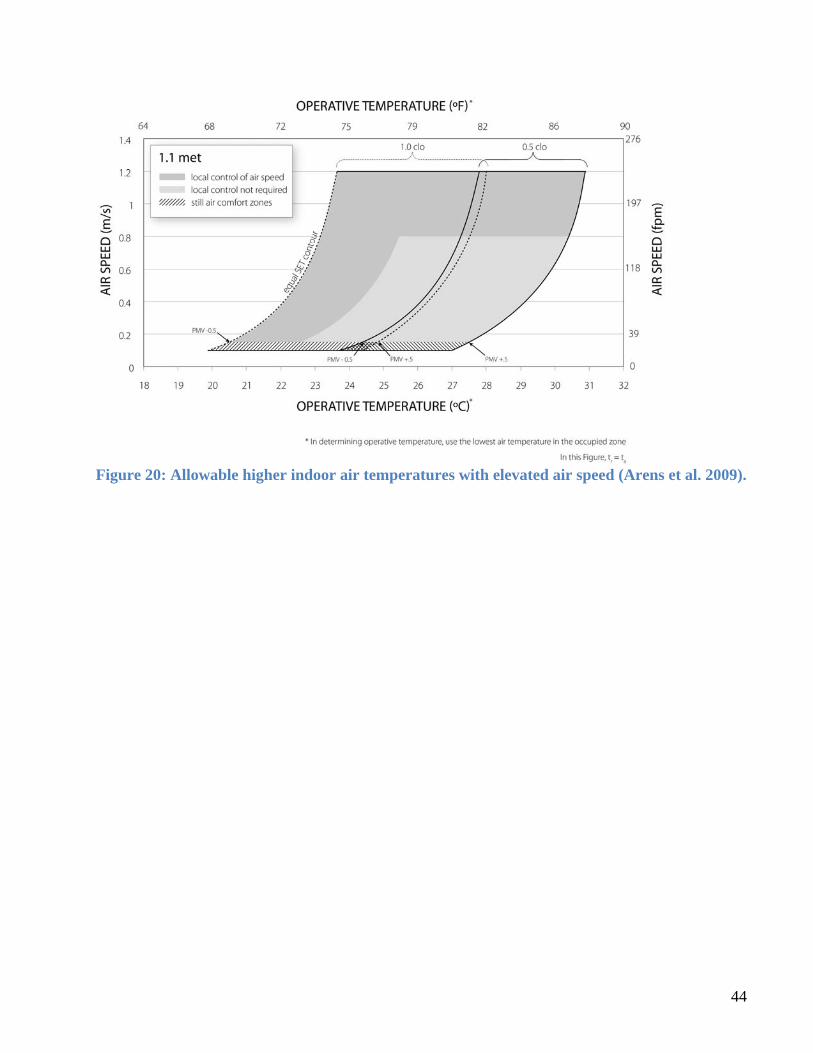
44

Figure 20: Allowable higher indoor air temperatures with elevated air speed (Arens et al. 2009).

APPENDIX R Appendix R: Appendix 11: Self-Correcting Controls For VAV Systems Faults

2087 Addison Street, 2nd Floor Berkeley, CA 94704-110

(510) 643-1440 uc-ciee.org

California Institute forEnergy and Environment

Self-Correcting Controls For VAV Systems Faults Filter/Fan/Coil and VAV Box Sections

Final Project Report May, 2011 Prepared by Pacific Northwest National Laboratory Prepared for CIEE Enabling Technologies Development Program Program Manager Gaymond Yee

i

PREFACE

This report documents work performed by Pacific Northwest National Laboratory for the California Institute for Energy Efficiency under subcontract PODR01-X08 between The Regents of the University of California and Battelle, Acting on behalf of Pacific Northwest National Laboratory.

DISCLAIMER

This report was prepared as the result of work sponsored by the California Energy Commission. It does not necessarily represent the views of the Energy Commission, its employees or the State of California. The Energy Commission, the State of California, its employees, contractors and subcontractors make no warrant, express or implied, and assume no legal liability for the information in this report; nor does any party represent that the uses of this information will not infringe upon privately owned rights. This report has not been approved or disapproved by the California Energy Commission nor has the California Energy Commission passed upon the accuracy or adequacy of the information in this report.

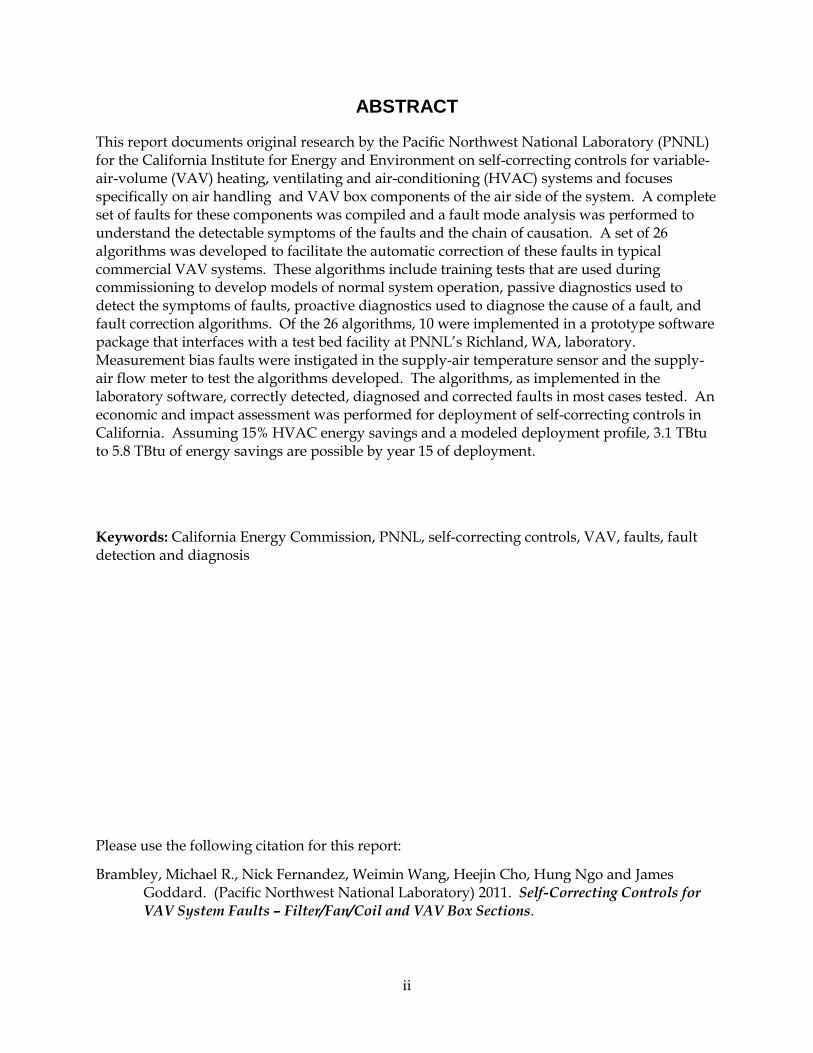
ii

ABSTRACT

This report documents original research by the Pacific Northwest National Laboratory (PNNL) for the California Institute for Energy and Environment on self-correcting controls for variable-air-volume (VAV) heating, ventilating and air-conditioning (HVAC) systems and focuses specifically on air handling and VAV box components of the air side of the system. A complete set of faults for these components was compiled and a fault mode analysis was performed to understand the detectable symptoms of the faults and the chain of causation. A set of 26 algorithms was developed to facilitate the automatic correction of these faults in typical commercial VAV systems. These algorithms include training tests that are used during commissioning to develop models of normal system operation, passive diagnostics used to detect the symptoms of faults, proactive diagnostics used to diagnose the cause of a fault, and fault correction algorithms. Of the 26 algorithms, 10 were implemented in a prototype software package that interfaces with a test bed facility at PNNL’s Richland, WA, laboratory. Measurement bias faults were instigated in the supply-air temperature sensor and the supply-air flow meter to test the algorithms developed. The algorithms, as implemented in the laboratory software, correctly detected, diagnosed and corrected faults in most cases tested. An economic and impact assessment was performed for deployment of self-correcting controls in California. Assuming 15% HVAC energy savings and a modeled deployment profile, 3.1 TBtu to 5.8 TBtu of energy savings are possible by year 15 of deployment.

Keywords: California Energy Commission, PNNL, self-correcting controls, VAV, faults, fault detection and diagnosis

Please use the following citation for this report:

Brambley, Michael R., Nick Fernandez, Weimin Wang, Heejin Cho, Hung Ngo and James Goddard. (Pacific Northwest National Laboratory) 2011. Self-Correcting Controls for VAV System Faults – Filter/Fan/Coil and VAV Box Sections.

iii

TABLE OF CONTENTS

PREFACE ..................................................................................................................................................... i

ABSTRACT ............................................................................................................................................... ii

TABLE OF CONTENTS ......................................................................................................................... iii

EXECUTIVE SUMMARY ........................................................................................................................ 1

Identify Faults ......................................................................................................................................... 1

Development of Self-correction Methods and Algorithms .............................................................. 1

Implementation of Algorithms in Software Code and Integration with the Control System ..... 2

Laboratory Testing of the Self-Correcting Software ......................................................................... 2

Economic and Impact Assessment of Deployment ........................................................................... 3

The Path Forward .................................................................................................................................. 3

CHAPTER 1: Fault Identification and Analysis .................................................................................. 4

System Description ................................................................................................................................ 4

Air-handling Unit (AHU) ................................................................................................................. 4

Variable-air-volume (VAV) Terminal Boxes .................................................................................. 6

Identification of potential faults ........................................................................................................... 8

Fault mode analysis ............................................................................................................................. 16

CHAPTER 2: Algorithm Development ............................................................................................... 24

Training ................................................................................................................................................. 28

Passive Diagnostics .............................................................................................................................. 28

Proactive Diagnostics .......................................................................................................................... 31

Fault Correction .................................................................................................................................... 34

CHAPTER 3: Implementation and Testing ........................................................................................ 37

Description of the Test Facility ........................................................................................................... 37

Implementation of Algorithms .......................................................................................................... 37

Results .................................................................................................................................................... 39

Analysis of Training Data ............................................................................................................... 39

Test Results ....................................................................................................................................... 41

CHAPTER 4: Economic and Impact Assessment .............................................................................. 50

Technical and Market Potential ......................................................................................................... 50

iv

Methodology ..................................................................................................................................... 51

Built-up System Savings ................................................................................................................. 52

Packaged System Savings ............................................................................................................... 55

Total Impacts on California Market .................................................................................................. 58

Economic Impact .............................................................................................................................. 59

Environmental Impacts ................................................................................................................... 60

CHAPTER 5: Future Work ..................................................................................................................... 62

Improved Training Models and Procedures .................................................................................... 62

Completion of Full Suite of Laboratory Tests .................................................................................. 63

Integrating with Additional BASs and Field Testing ..................................................................... 65

Path Forward ........................................................................................................................................ 65

REFERENCES .......................................................................................................................................... 67

1

EXECUTIVE SUMMARY The Pacific Northwest National Laboratory (PNNL) performed research for the California Institute for Energy and Environment (CIEE) in self-correcting controls for commercial building VAV systems. The work included identification and analysis of fault modes and their symptoms, developing algorithms for the four steps of the process leading to automated correction of faults not requiring human intervention to physically repair or replace a system component, coding a selected subset of the algorithms in prototype laboratory-grade software, and laboratory testing. These steps in the process include training to capture relationships among key variables, fault detection, fault diagnosis (which is also known as fault isolation), and fault correction. The remainder of this executive summary briefly describes the work performed and key results and is organized in parallel to the chapter structure of the report.

Identify Faults A comprehensive list of faults that affect VAV systems was developed and mapped to their potential causes to facilitate the development of algorithms. The list of faults was developed in a brainstorming session that brought together several experts with experience in diagnosing faults in HVAC systems and developing automated HVAC control and fault detection and diagnostic (FDD) systems. The faults were categorized as hard (physical) or soft (software) component faults. The components for which faults were identified include temperature, pressure, and air-flow rate sensors, valves, dampers, fans, filters, coils, economizers, VAV boxes, and supply-fan controls. Through a process called fault mode analysis, these faults were mapped to observable symptoms, which are indicators of deviations from expected system behavior. Some of these symptoms are easily observable (for example, if the measured supply-air temperature is colder than the mixed-air temperature when the coiling-cool valve in an air-handler has been commanded closed.) Other faults require the development of more complex models to empirically define normal operating conditions.

A total of 28 faults were identified that can be diagnosed in the air-handler (filter/fan/coil) and VAV-box sections of the air side of VAV systems in this set of algorithms. Of these, 18 are automatically correctable soft faults, and 10 are hard faults that require physical repair or replacement.

Development of Self-correction Methods and Algorithms Based on physical principles, equipment design, and the insights gained from the fault-mode analysis, a set of rule-based algorithms was developed to facilitate automatic correction of the identified faults. The structure for these algorithms is the same structure used previously by PNNL in development of self-correcting controls for the mixing-box section of air handlers. This structure is a four-step process to fault correction. The first step, training, establishes the normal range for a set of variables and quantitative empirical relationships among some for later use in fault detection and diagnosis. The next step, passive fault detection (or passive diagnostics) uses observation of fault symptoms during ordinary operation to detect when a fault has occurred. After a fault is detected, proactive diagnostics (tests) are used to isolate

2

which of potentially several possible faults was responsible for the observed symptom. This typically requires more information than is available from normal operation of the system, so specific diagnostic tests are run to create situations that provide additional data and information. After the fault has been isolated, the fault correction process characterizes the fault (e.g., the magnitude of a constant bias in a sensor output rather than erratic, constantly changing, sensor output), formulates a mathematical description of the fault, and then subtracts the fault to compensate the behavior of the faulty device. The correction is implemented via a virtual point (e.g., sensor output, control signal, etc.). The algorithms are documented in detail in a companion report identified in the reference list of this report as Fernandez et al. 2011.

Implementation of Algorithms in Software Code and Integration with the Control System The algorithms were successfully coded in prototype software using the Jython programming language (a hybrid of Java and Python). A subset of the full suite of algorithms was coded. Priority was given to the development of all four steps of the fault-correction process for two key soft faults: biased supply-air flow-rate sensors and biased supply-air temperature sensors. The software was integrated with a Johnson Metasys Building Automation System, using Factory Plant Management Interface (FPMI) software. The software uses two sets of virtual points for sensors. The first enables simulation of sensor faults through virtual sensor points that the control system reads in lieu of the direct sensor measurements. These virtual sensor points enable instigation of faults without damaging equipment and the outputs of these virtual sensors exhibit the characteristics of the fault of interest. The other virtual sensor points enable application of corrections developed by the self-correcting algorithms to the faulty sensor signals to create corrected sensor signals that replace erroneous values to the control algorithms.

Laboratory Testing of the Self-Correcting Software Six laboratory tests were performed. Three tests of supply-air flow-rate sensor bias and three tests of biased supply-air temperature sensors were performed. The three tests for each fault were used to investigate differences in the outcome of the test as functions of fault severity and the values of key selectable thresholds for fault detection. The tests were each initiated with a 5-minute period of fault-free operation, during which no faults were detected. In all tests, the passive diagnostic tests successfully detected a fault soon after its instigation. In four tests, the fault was correctly diagnosed, and automatically corrected approximately to the level of the instigated bias. Faults with low severity and higher detection thresholds presented problems, which led to an inconclusive result for one test of the biased supply-air temperature sensor and an incorrect fault determination for one test for the biased supply-air flow-rate sensor. Modest changes in the algorithms are proposed to account for these issues. All methods for fault detection and diagnosis impose a tradeoff between sensitivity and false positive fault detection. Generally, as sensitivity is increased, the probability of false positives increases. Therefore, achieving the right balance between these behaviors is critical to successful deployment of the technology. Further laboratory testing will be used to “tune” the associated variables (e.g., detection thresholds and sensor tolerances).

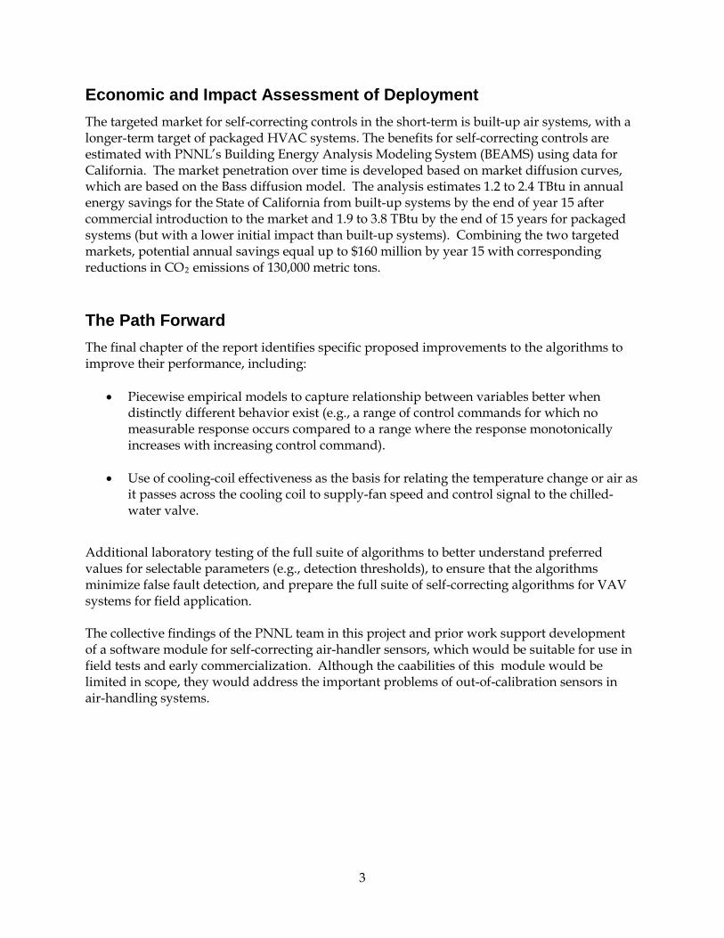
3

Economic and Impact Assessment of Deployment The targeted market for self-correcting controls in the short-term is built-up air systems, with a longer-term target of packaged HVAC systems. The benefits for self-correcting controls are estimated with PNNL’s Building Energy Analysis Modeling System (BEAMS) using data for California. The market penetration over time is developed based on market diffusion curves, which are based on the Bass diffusion model. The analysis estimates 1.2 to 2.4 TBtu in annual energy savings for the State of California from built-up systems by the end of year 15 after commercial introduction to the market and 1.9 to 3.8 TBtu by the end of 15 years for packaged systems (but with a lower initial impact than built-up systems). Combining the two targeted markets, potential annual savings equal up to $160 million by year 15 with corresponding reductions in CO2 emissions of 130,000 metric tons.

The Path Forward The final chapter of the report identifies specific proposed improvements to the algorithms to improve their performance, including:

• Piecewise empirical models to capture relationship between variables better when distinctly different behavior exist (e.g., a range of control commands for which no measurable response occurs compared to a range where the response monotonically increases with increasing control command).

• Use of cooling-coil effectiveness as the basis for relating the temperature change or air as

it passes across the cooling coil to supply-fan speed and control signal to the chilled-water valve.

Additional laboratory testing of the full suite of algorithms to better understand preferred values for selectable parameters (e.g., detection thresholds), to ensure that the algorithms minimize false fault detection, and prepare the full suite of self-correcting algorithms for VAV systems for field application. The collective findings of the PNNL team in this project and prior work support development of a software module for self-correcting air-handler sensors, which would be suitable for use in field tests and early commercialization. Although the caabilities of this module would be limited in scope, they would address the important problems of out-of-calibration sensors in air-handling systems.

4

CHAPTER 1: Fault Identification and Analysis This chapter includes three sections. In the first section, the typical single-duct variable-air-volume (VAV) air-handling unit (AHU) and the VAV terminal boxes are briefly described, along with operating modes and sequences of control. Potential faults are presented in the second section for each component of the VAV system, and in the third section, a number of cause-effect diagrams are used to associate fault symptoms to the faults themselves, which are identified in the second section.

System Description The single-duct, VAV air-handling and distribution system is described in this section with the AHU and VAV terminal boxes described separately. The AHU receives return air from the building zones, recirculates a fraction of it and exhausts the rest to the outdoors. The recirculated air mixes with outdoor air in the mixing box. The mixed air is then filtered, cooled (or heated), and then distributed to the terminal boxes, which further control the air-flow to each zone and reheat the supply-air, if necessary.

Air-handling Unit (AHU) Figure 1 is a schematic diagram of a generic single-duct AHU for VAV systems. Typical sensors are identified by labeled, colored circles (see the key in the lower-right in the figure).

Figure 1: Diagram of a Typical VAV Air-handling Unit

Outdoor air (OA) enters the AHU, passing through the outdoor-air damper, and is mixed with the air returned from the space via a return fan. The mixed air sequentially passes through the

dP

dPF

Mixing Box HC CC

Variable Speed Supply

Fan

To VAV boxes

Return Fan

Temperature or combined temperature and humidity sensor

PS

T/RHRA

TMA

Pressure sensor

Differential pressure sensor

Chilled waterHot water

Outdoor air (OA)

Exhaust air

Return air (RA)

THC

THW

Air flow rate station

TCW

P

T/RH

T/RHOa

V

TSA VS

Filter

5

filter, the heating coil (HC), if present, and the cooling coil (CC), which are used to maintain the supply-air at a predefined temperature set point in the supply duct downstream of the supply fan. In practice, the supply fan may be located either upstream of the coils (blow through) or downstream of the coils (draw through, as shown in Figure 1). In many systems, only a cooling coil is present. The supply-fan speed is modulated to maintain the supply-air static pressure at a set point. The return-fan speed is set according to the building’s pressurization requirement and the speed of the supply fan.

When the AHU is in operation during occupied periods, it may work in one of four operating modes: heating with minimum outdoor OA, economizing (with OA used for cooling), mechanical cooling with full economizing (100% OA), and mechanical cooling with minimum OA. The specific mode used depends on the outdoor-air conditions. The modes are shown graphically in Figure 2 and are described below.

Figure 2: Air Handler Operating Modes

Heating mode

In this mode, the OA temperature is low enough that the mixed-air (MA) temperature is lower than the supply-air temperature set point, even if the OA damper is at the minimum position required to meet ventilation requirements. Thus, the heating coil valve is controlled to an open position to heat the supply air to its set point, while the cooling coil valve is fully closed, and the OA damper is kept at its minimum position.

Heating mode

Economizing mode

Mechanical cooling with 100% OA

Mechanical cooling with minimum OA

Con

trol S

igna

l (%

)

0

100

OA damper

Cooling coil valveHeating coil valve

Outdoor Air Temperature

6

Economizing (OA cooling) mode

At higher OA temperatures, the AHU changes from the heating mode to cooling with OA (i.e., economizing with no mechanical cooling). In this mode, both the heating-coil and the cooling-coil valves are closed and the supply-air temperature is maintained at its set point by modulating the mixing-box dampers (opening the outdoor-air damper and closing the return-air damper as the need for cooling increases).1

Mechanical cooling with full economizing (100% OA mode)

As the cooling load continues to increase, the OA damper opens until it reaches its maximum open position, provided the OA temperature (or enthalpy) remains sufficiently low to provide cooling. If economizing with 100% OA cannot lower the MA temperature to the supply-air set point, mechanical cooling is initiated by modulating the cooling-coil valve open sufficiently to lower the supply-air temperature to its set point to meet the load that economizing cannot meet. This mode of economizing is frequently referred to as integrated. The heating coil valve is kept completely closed in this operating mode. Some economizer controls, known as non-integrated, do not simultaneously use economizing and mechanical cooling. These systems do not enter the mechanical cooling with full economizing mode.

Mechanical cooling with minimum OA mode

When the OA temperature (or enthalpy) increases above the return-air temperature (or enthalpy) or other pre-specified limit, the OA damper modulates back to its minimum position for ventilation, and mechanical cooling is used to meet the entire cooling load. The cooling coil valve is modulated to provide the required mechanical cooling, while the heating coil valve is kept completely closed.

Variable-air-volume (VAV) Terminal Boxes VAV boxes are an integrated part of the VAV system. In contrast to the air-handling unit, VAV terminal units have more varied types such as fan-powered terminal units, induction terminal units, and throttling VAV terminal units with or without reheating. In the current stage of this project, the fault analysis focuses on the single-duct, pressure-independent throttling VAV box with hydronic reheat as shown in Figure 3. This box captures many of the features of simpler terminal boxes, which can be modeled by deleting features of this box (e.g., terminal reheat). For the VAV box shown in Figure 3, the controller modulates the damper to meet thermal load requirements. A minimum air flow rate is preset to satisfy space ventilation. The valve can modulate the hot-water flow rate to the reheat coil to raise the temperature of the supply air to moderate cooling or to provide heat to the space.

These VAV terminal boxes work in one of three operating modes: cooling with more than the minimum air flow rate, deadband mode, and reheating. The specific mode of operation

1 Economizing may be controlled on dry-bulb temperature or enthalpy.

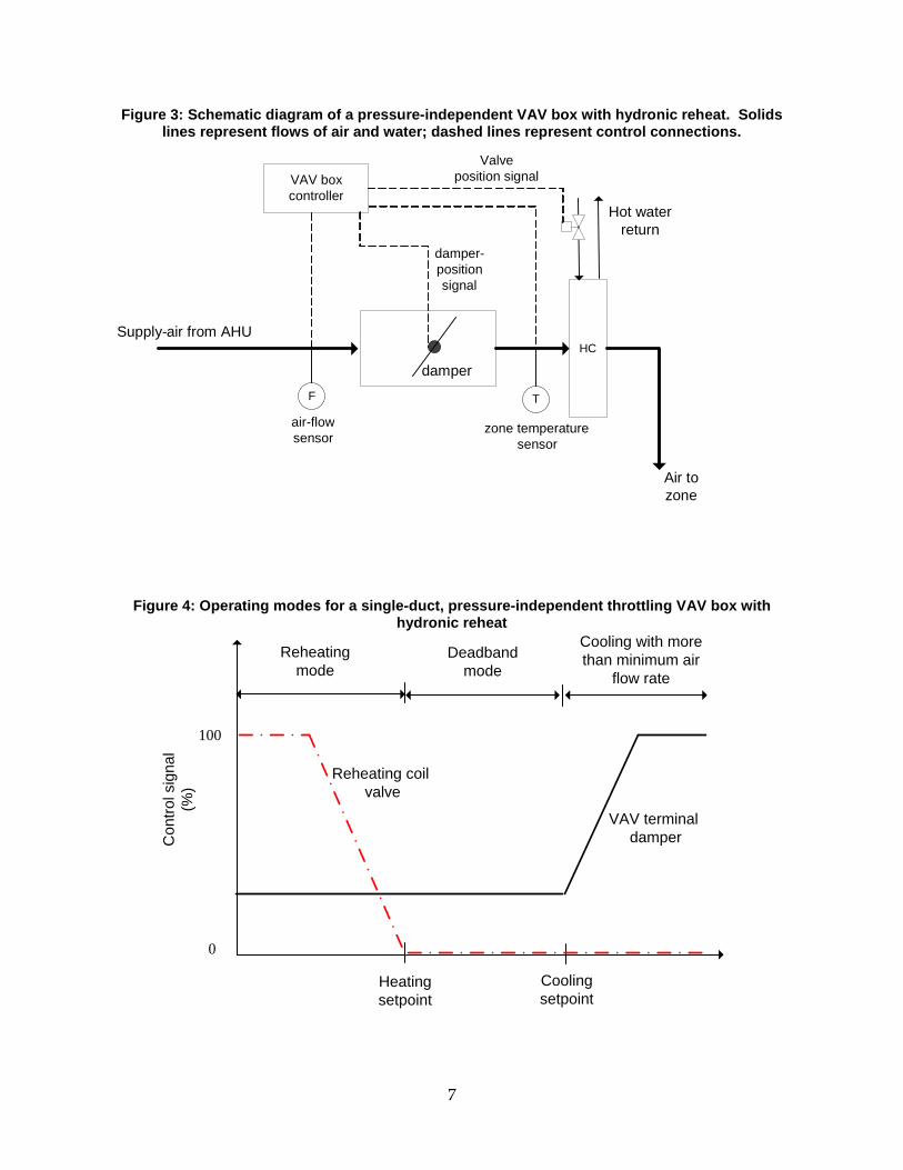
7

Figure 3: Schematic diagram of a pressure-independent VAV box with hydronic reheat. Solids lines represent flows of air and water; dashed lines represent control connections.

Figure 4: Operating modes for a single-duct, pressure-independent throttling VAV box with hydronic reheat

Reheating mode

Deadband mode

Cooling with more than minimum air

flow rate

Con

trol s

igna

l (%

)

0

100

VAV terminal damper

Reheating coil valve

Cooling setpoint

Heating setpoint

HC

VAV box controller

Air to zone

Supply - air from AHU

damper

Hot water return

T

zone temperature sensor

F air - flow sensor

damper - position signal

Valve position signal

8

depends on the zone-air temperature. The operating modes are shown graphically in Figure 4 and are described below.

Cooling with more than the minimum air flow rate

The VAV box operates in this mode when the zone-air temperature increases above the space cooling set point. In this case, the air flow rate is increased by increasing the damper opening. The reheat coil valve is kept closed.

Deadband mode

The VAV box operates in this mode when the zone-air temperature lies between the space cooling and heating set points. The air flow rate is maintained at the minimum value to meet the ventilation requirement, and the reheat coil valve is kept closed.

Reheating

The VAV box enters this mode when the zone-air temperature decreases below the space heating set point. In this case, the valve for the reheat coil modulates to meet the space heating load. The air flow rate may be kept constant at its minimum value or the VAV damper may open further to meet additional space heating load after the reheat valve has opened 100%.

Identification of potential faults Potential faults in air-handling units and the associated VAV terminal boxes can be identified in two steps. First, a preliminary list of potential faults was prepared based on review of the literature on fault detection and diagnostics (FDD) for AHUs and VAV boxes (see, e.g., Fernandez et al. 2009a; Fernandez et al. 2009b; Dexter and Pakanen 2001; Hyvarinen and Karki 1996; Smith and Bushby 2003). The literature has generally focused on detection and diagnosis for a number of common faults (e.g., sensor biases and control logic errors). Little attention has been given to developing a comprehensive list of potential faults and the causes of those faults. Therefore, a second step was used to address this limitation and identify a more complete set of faults and their potential causes. A group of eight researchers identified and discussed additional faults and underlying causes observed in the field to develop a complete set of symptoms, faults and underlying causes. The field experience of each participant in HVAC system implementation, maintenance and troubleshooting varied from approximately 2 years to over 30 years.

HVAC faults can be classified into different categories according to criteria such as complete component failure versus performance degradation, hardware faults versus software faults, and self-correctable faults versus faults requiring human corrective action. Because this work is performed in the context of self-correcting HVAC control, each fault is categorized as self-correctable (SC), possibly self-correctable (PSC), and not self-correctable (NSC). A SC fault is one that can be corrected through changes in the values of parameters or to software code in the control system. These faults include, for example, incorrect schedules, poorly chosen set points, continually oscillating (or hunting) controls, incorrectly implemented controls, and failed or out-of-calibration sensors. A PSC fault is one for which self correction may be feasible under certain circumstances, one for which the team is presently uncertain that self correction can be implemented, or a fault that may be correctable if additional sensors were installed beyond

9

those ordinarily present on the HVAC system. An NSC fault is one for which restoration to normal system performance from the faulty situation is not possible without physical repair of the system, which requires human intervention.2

The potential faults for the VAV air-handling system described earlier in this chapter are identified in Table 1 through Table 4. Each table presents the faults for one of the major parts comprising the VAV system: air-mixing section, filter-coil section, fan section, and VAV boxes. The categorization of each fault is given in the right-most column of each table, using the abbreviations SC, PSC and NSC.

2 NSC faults generally result from physical failure of components, but all physical faults are not NSC faults. In fact, as stated in the text, some physical faults, such as complete failure of some sensors, can be automatically corrected. Furthermore, compensation for some physical faults that improves performance of the system above the performance that would occur by default when a physical fault or failure occurs may be possible. Such fault compensation will be considered in future research.

10

Table 1: Air-Mixing Section Faults

Components Type of Fault/Failure

Specific Fault Fault Category (SC, PSC or NSC)*

Temperature or humidity sensors (return air—RA, outdoor air—OA, mixed-air—MA)

Complete failure—no signal

SC

Constant bias in signal

Sensor out of calibration SC

Sensor installation location fault

PSC

Wiring fault SC

Long lead wires SC

Time varying bias in signal

Sensor installation of location fault

PSC

Drifting signal SC

Intermittent signal Communication problems such as a wiring fault

PSC

Sensor internal fault PSC

Wiring fault (e.g., bad solder joint)

PSC

Randomly varying signal

Communication problems such as a wiring fault

PSC

Sensor internal fault PSC

Induced electrical noise PSC

Damper and actuator

Stuck damper (fully open, completely closed, intermediate position)

Damper motor failure NSC

Damper linkage broken or disconnected

NSC

Damper or linkage stuck from rust or other corrosion

NSC

Wire to actuator disconnected or no power

NSC

Controller in manual mode PSC

Air leakage when damper is fully closed

Damper blade damaged NSC

Poor damper seals NSC

Damper not closing completely

PSC

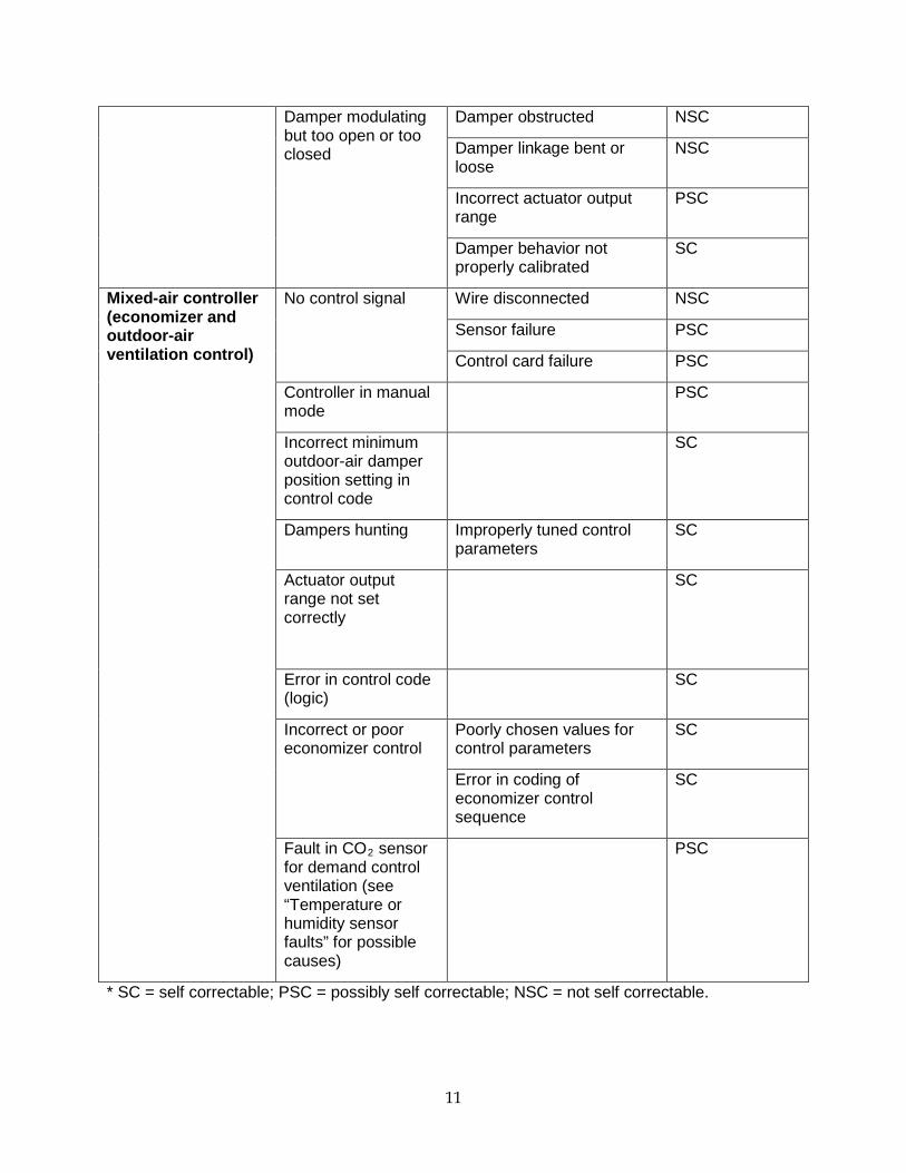
11

Damper modulating but too open or too closed

Damper obstructed NSC

Damper linkage bent or loose

NSC

Incorrect actuator output range

PSC

Damper behavior not properly calibrated

SC

Mixed-air controller (economizer and outdoor-air ventilation control)

No control signal Wire disconnected NSC

Sensor failure PSC

Control card failure PSC

Controller in manual mode

PSC

Incorrect minimum outdoor-air damper position setting in control code

SC

Dampers hunting Improperly tuned control parameters

SC

Actuator output range not set correctly

SC

Error in control code (logic)

SC

Incorrect or poor economizer control

Poorly chosen values for control parameters

SC

Error in coding of economizer control sequence

SC

Fault in CO2 sensor for demand control ventilation (see “Temperature or humidity sensor faults” for possible causes)

PSC

* SC = self correctable; PSC = possibly self correctable; NSC = not self correctable.

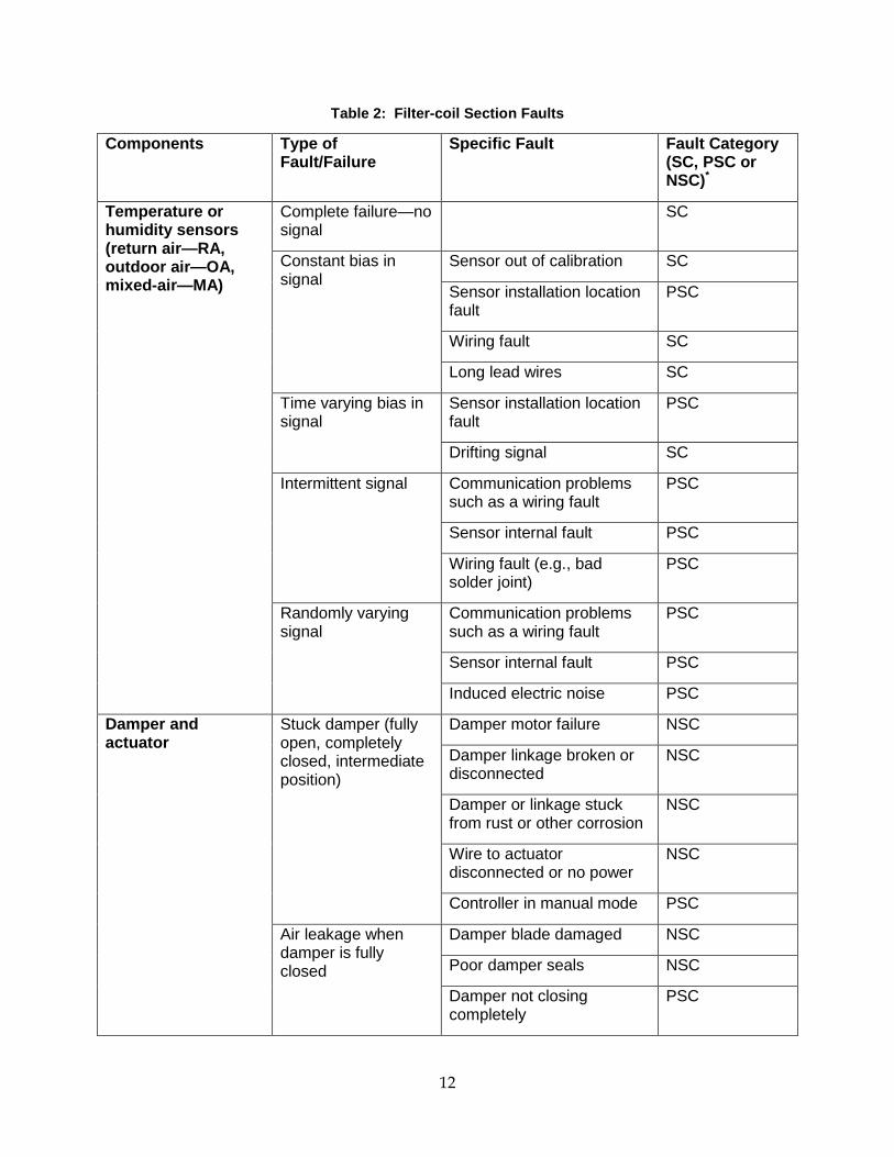
12

Table 2: Filter-coil Section Faults

Components Type of Fault/Failure

Specific Fault Fault Category (SC, PSC or NSC)*

Temperature or humidity sensors (return air—RA, outdoor air—OA, mixed-air—MA)

Complete failure—no signal

SC

Constant bias in signal

Sensor out of calibration SC

Sensor installation location fault

PSC

Wiring fault SC

Long lead wires SC

Time varying bias in signal

Sensor installation location fault

PSC

Drifting signal SC

Intermittent signal Communication problems such as a wiring fault

PSC

Sensor internal fault PSC

Wiring fault (e.g., bad solder joint)

PSC

Randomly varying signal

Communication problems such as a wiring fault

PSC

Sensor internal fault PSC

Induced electric noise PSC

Damper and actuator

Stuck damper (fully open, completely closed, intermediate position)

Damper motor failure NSC

Damper linkage broken or disconnected

NSC

Damper or linkage stuck from rust or other corrosion

NSC

Wire to actuator disconnected or no power

NSC

Controller in manual mode PSC

Air leakage when damper is fully closed

Damper blade damaged NSC

Poor damper seals NSC

Damper not closing completely

PSC

13

Damper modulating but too open or too closed

Damper obstructed NSC

Damper linkage bent or loose

NSC

Incorrect actuator output range

PSC

Damper behavior not properly calibrated

SC

Mixed-air controller (economizer and outdoor-air ventilation control)

No control signal Wire disconnected NSC

Sensor failure PSC

Control card failure PSC

Controller in manual mode

PSC

Incorrect minimum outdoor-air damper position setting in control code

SC

Dampers hunting Improperly tuned control parameters

SC

Actuator output range incorrectly set

SC

Error in control code (logic)

SC

Incorrect or poor economizer control

Poorly chosen values for control parameters

SC

Error in coding of economizer control sequence

SC

Fault in CO2 sensor for demand control ventilation (see “Temperature or humidity sensor faults” for possible causes)

PSC

* SC = self correctable; PSC = possibly self correctable; NSC = not self correctable.

14

Table 3: Fan Section Faults

Components Type of Fault/Failure

Specific Fault Fault Category (SC, PSC or

NSC)* Fan (supply fan-SF, return fan-RF)

Complete failure Power disconnected NSC Blown fuse NSC

Off for protection (design safety measures)

NSC

Decrease in fan efficiency

Dirt accumulation NSC Loose fan blade NSC Other efficiency degradation

NSC

Pressure sensor (supply-air duct; see “Temperature or humidity sensor faults” in Table 1 for detailed fault or causes)

Complete failure PSC Biased signal PSC Drifting signal PSC Intermittent signal PSC Randomly varying signal

PSC

Supply and return fan controller

No control signal Wire disconnected NSC Sensor failure PSC Controller card failure NSC

Improperly tuned control parameters

SC

Improper set point for supply-air duct pressure

SC

Controller software and parameter value faults

Improper value for supply-air temperature set point

SC

Error in control code (logic) SC Actuator output range not set correctly

SC

Inappropriate override of automatic operation (e.g., variable flow rate bypass mode on)

SC

* SC = self correctable; PSC = possibly self correctable; NSC = not self correctable.

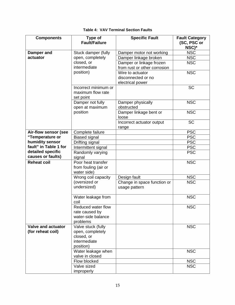
15

Table 4: VAV Terminal Section Faults

Components Type of Fault/Failure

Specific Fault Fault Category (SC, PSC or

NSC)* Damper and actuator

Stuck damper (fully open, completely closed, or intermediate position)

Damper motor not working NSC Damper linkage broken NSC Damper or linkage frozen from rust or other corrosion

NSC

Wire to actuator disconnected or no electrical power

NSC

Incorrect minimum or maximum flow rate set point

SC

Damper not fully open at maximum position

Damper physically obstructed

NSC

Damper linkage bent or loose

NSC

Incorrect actuator output range

SC

Air-flow sensor (see “Temperature or humidity sensor fault” in Table 1 for detailed specific causes or faults)

Complete failure PSC Biased signal PSC Drifting signal PSC Intermittent signal PSC Randomly varying signal

PSC

Reheat coil Poor heat transfer from fouling (air or water side)

NSC

Wrong coil capacity (oversized or undersized)

Design fault NSC Change in space function or usage pattern

NSC

Water leakage from coil

NSC

Reduced water flow rate caused by water-side balance problems

NSC

Valve and actuator (for reheat coil)

Valve stuck (fully open, completely closed, or intermediate position)

NSC

Water leakage when valve in closed

NSC

Flow blocked NSC Valve sized improperly

NSC

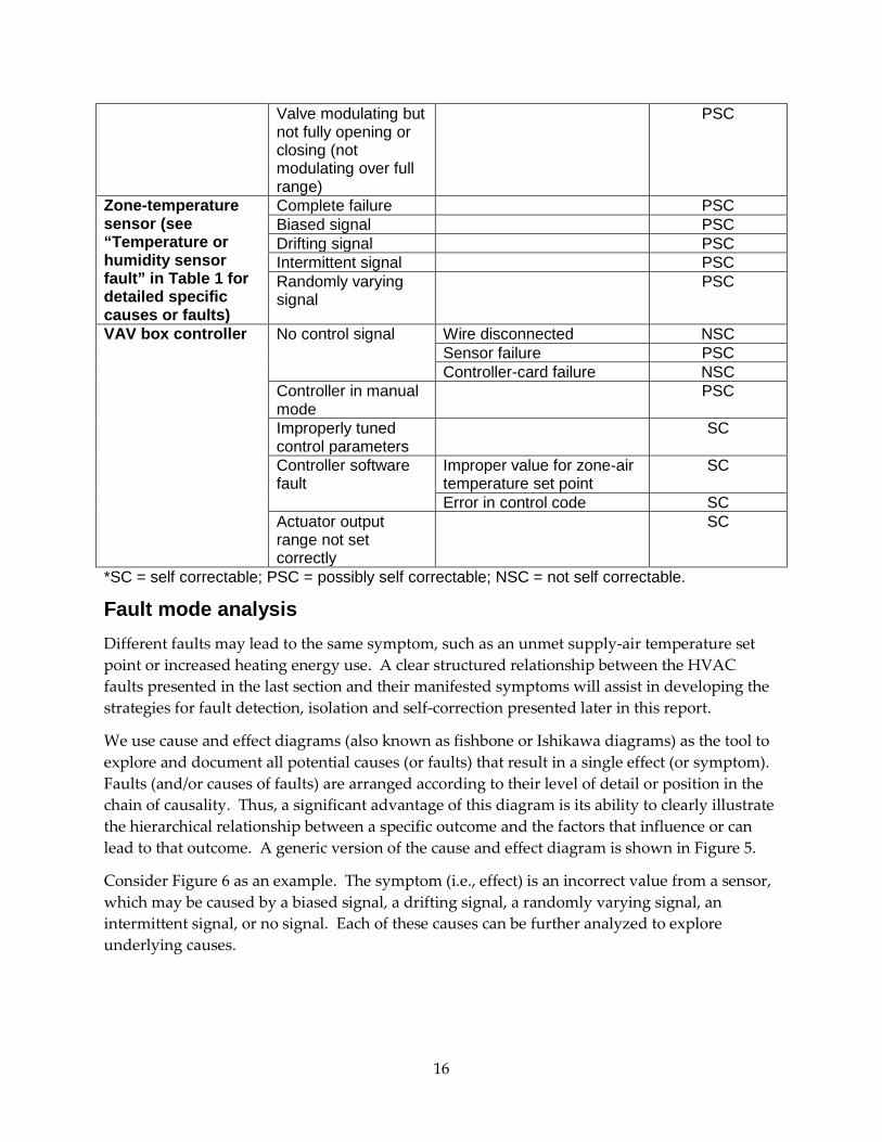
16

Valve modulating but not fully opening or closing (not modulating over full range)

PSC

Zone-temperature sensor (see “Temperature or humidity sensor fault” in Table 1 for detailed specific causes or faults)

Complete failure PSC Biased signal PSC Drifting signal PSC Intermittent signal PSC Randomly varying signal

PSC

VAV box controller No control signal Wire disconnected NSC Sensor failure PSC Controller-card failure NSC

Controller in manual mode

PSC

Improperly tuned control parameters

SC

Controller software fault

Improper value for zone-air temperature set point

SC

Error in control code SC Actuator output range not set correctly

SC

*SC = self correctable; PSC = possibly self correctable; NSC = not self correctable.

Fault mode analysis Different faults may lead to the same symptom, such as an unmet supply-air temperature set point or increased heating energy use. A clear structured relationship between the HVAC faults presented in the last section and their manifested symptoms will assist in developing the strategies for fault detection, isolation and self-correction presented later in this report.

We use cause and effect diagrams (also known as fishbone or Ishikawa diagrams) as the tool to explore and document all potential causes (or faults) that result in a single effect (or symptom). Faults (and/or causes of faults) are arranged according to their level of detail or position in the chain of causality. Thus, a significant advantage of this diagram is its ability to clearly illustrate the hierarchical relationship between a specific outcome and the factors that influence or can lead to that outcome. A generic version of the cause and effect diagram is shown in Figure 5.

Consider Figure 6 as an example. The symptom (i.e., effect) is an incorrect value from a sensor, which may be caused by a biased signal, a drifting signal, a randomly varying signal, an intermittent signal, or no signal. Each of these causes can be further analyzed to explore underlying causes.

17

Figure 5: Generic Cause and Effect Diagram Adapted for Application to Equipment Faults

Figure 6: Cause-effect Diagram for an Incorrect Sensor Measurement

Because an HVAC symptom is an observed deviation from normal (or expected) operation, it is convenient to select the directly measured variables, control signals and easily derived variables as indicators of symptoms. Cause-effect diagrams are presented for a total of 11 symptoms (effects) in Figure 6 through Figure 16. The symptoms for which cause-effect diagrams are shown are:

• Sensor measurement is not correct

• MA temperature differs from normal values under similar operating conditions

Effect

Fault 2

Fault 4

Fault 1

Fault 3

Primary cause 1

Primary cause 2

secondary cause 1

secondary cause 2

Reference diagramsecondary

cause 1

Sensor measurement is not correct

Intermittent signal

Biased signal

Wiring fault

Randomly varying signal

Induced electric noise

No signal

Wiring disconnected

Sensor internal fault

Sensor out of calibration

Sensor installation faultSensor location fault

Wiring fault

Long wiringInappropriate sensor type

range

time constant

Sensor internal fault

Wiring fault

Sensor internal fault

Incorrect power supply

Drifting signal

Sensor out of calibration

Inappropriate sensor type

18

• Supply-air temperature differs from its set point

• Supply-air pressure differs from its set point

• AHU operation mode changes more frequently than normal

• Supply-air flow rate differs from normal values under similar operating conditions

• Supply-fan energy use differs from normal values under similar operating conditions

• AHU heating energy use differs from normal values under similar operating conditions

• AHU cooling energy use differs from normal values under similar operating conditions

• Zone-air temperature differs from its set point

• VAV box flow rate differs from normal values under similar operating conditions.

Cross references to fault analyses for different symptoms are used in Figure 6 through Figure 16 to make the cause-effect diagrams clearer and more legible. For example, Figure 7 refers to Figure 6 regarding the possible faults for temperature sensors, humidity sensors and CO2 sensors.

The cause-effect diagrams are tools used for formulating algorithms for self correction of amenable faults in air handlers and VAV terminal boxes in Chapter 2.

Figure 7: Cause-effect Diagram for the Mixed-air Temperature Differing from Values Normally Occurring Under Similar Operating Conditions

MA temperature differs from that at normal similar

operating conditions

Damper and actuator

Damper leakage at closed position

Damper modulating buttoo open or too closed

at a given position

MA, OA or RA temperature sensor

See Figure 6:Sensor fault

mode analysis

OA or RA humidity sensor(for enthalpy-based economizer)

See Figure 6:Sensor fault

mode analysis

Stuck damper

damper motor

damper linkage(broken, rusty)

wire to actuator disconnected

poor damper seals

damper blade damaged

incorrect actuator output range

bent or loose linkage

damper obstructed

Mixed air controller

No control signal

control card failure

wiring disconnected

Controller software

sequence logic

wrong value for min. position in control code

Poor control parameters tuning Inappropriate operation

override

CO2 sensor(for AHUs with demand controlled ventilation)

See Figure 6:Sensor fault

mode analysis

19

Figure 8: Cause-effect Diagram for the Supply-air Temperature Deviating from its Set Point

Figure 9: Cause-effect Diagram for the Supply-air Pressure Differing from its Set Point

Supply air temperature differs from its setpoint

Valve and actuator

Supply air temperature sensor

Valve leakage

Valve stuck

Valve not sized properly

Coils

Undersized coilcapacity

design problem

space functionality or usage pattern change

Water leakage in the coil

Supply air temperature controller

No control signal

See Figure 6:Sensor fault

mode analysis

Valve blocked

Fouling

Less water flow rate due to water-side balance problems

wiring disconnected

control card failureController software

sequence logic

improper temperature setpointWrong MA temperature

sensor signal to shutoff AHU

MA sensor location

air stratification

Poor control parameters tuning

Inappropriate operation override

OA damper

See Figure 7:MA temperature

different fault analysis

Higher OA flow rate when it should be at the minimum

Supply air pressurediffers from its setpoint

Supply fan controller

Pressure sensor

No control signal

control card failure

wiring disconnected

Controller software

sequence logic

inappropriate pressure setpoint

Poor control parameters tuning Inappropriate operation

override

Supply fan

Complete failure

disconnected blown fuse

motor failurebelt off

Fan stuck at certain speed

Filter

clogged

See Figure 6:Sensor fault

mode analysis

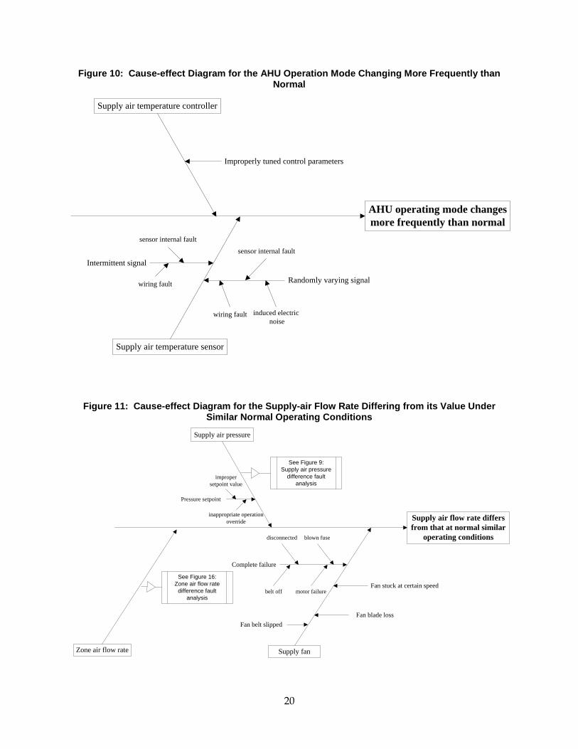
20

Figure 10: Cause-effect Diagram for the AHU Operation Mode Changing More Frequently than Normal

Figure 11: Cause-effect Diagram for the Supply-air Flow Rate Differing from its Value Under Similar Normal Operating Conditions

AHU operating mode changesmore frequently than normal

Supply air temperature sensor

Supply air temperature controller

Randomly varying signal

sensor internal fault

wiring fault induced electric noise

Intermittent signal

sensor internal fault

wiring fault

Improperly tuned control parameters

Supply air flow rate differsfrom that at normal similar

operating conditions

Supply air pressure

Supply fan

Complete failure

disconnected blown fuse

motor failurebelt offFan stuck at certain speed

See Figure 9:Supply air pressure

difference fault analysis

Pressure setpoint

improper setpoint value

inappropriate operation override

Fan blade lossFan belt slipped

Zone air flow rate

See Figure 16:Zone air flow rate

difference fault analysis

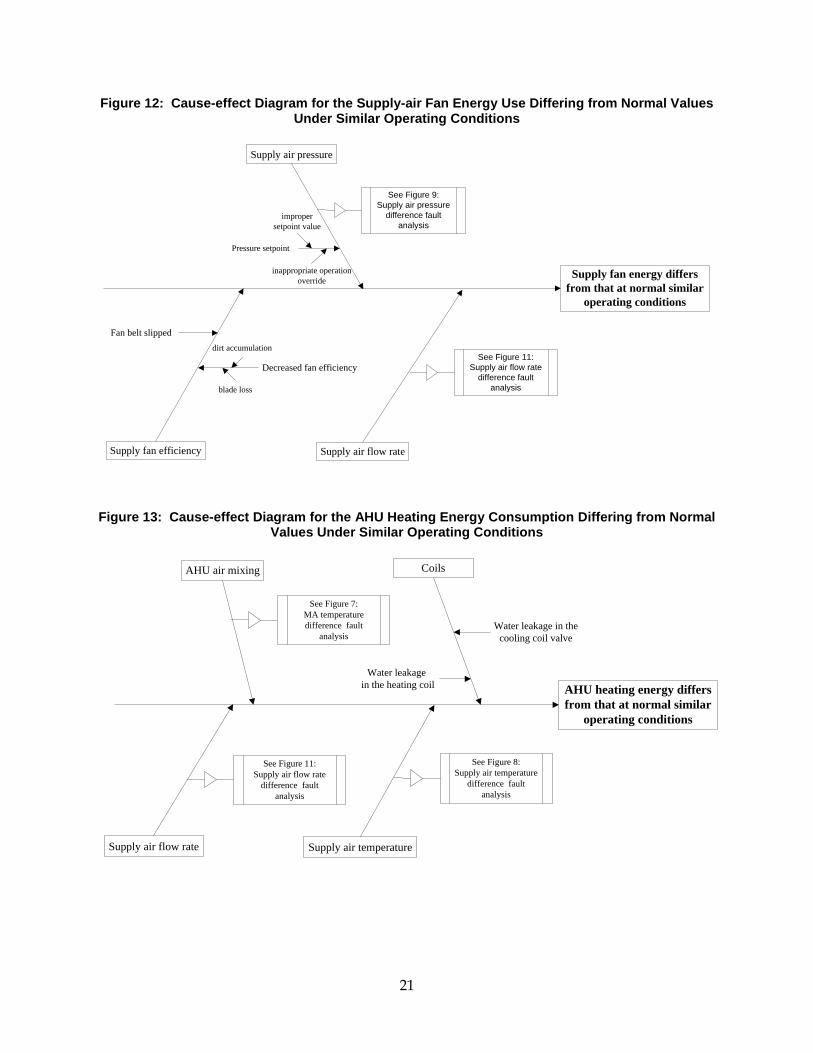
21

Figure 12: Cause-effect Diagram for the Supply-air Fan Energy Use Differing from Normal Values Under Similar Operating Conditions

Figure 13: Cause-effect Diagram for the AHU Heating Energy Consumption Differing from Normal Values Under Similar Operating Conditions

Supply fan energy differsfrom that at normal similar

operating conditions

Supply air pressure

Supply air flow rate

See Figure 9:Supply air pressure

difference fault analysis

Pressure setpoint

improper setpoint value

inappropriate operation override

See Figure 11:Supply air flow rate

difference fault analysis

Supply fan efficiency

Decreased fan efficiency

dirt accumulation

blade loss

Fan belt slipped

AHU heating energy differsfrom that at normal similar

operating conditions

Coils

Supply air temperature

See Figure 8:Supply air temperature

difference fault analysis

Supply air flow rate

See Figure 11:Supply air flow rate

difference fault analysis

Water leakage in the heating coil

Water leakage in thecooling coil valve

AHU air mixing

See Figure 7:MA temperature difference fault

analysis

22

Figure 14: Cause-effect Diagram for the AHU Cooling Energy Use Differing from Normal Values Under Similar Operating Conditions

Figure 15: Cause-effect Diagram for Zone-air Temperature Differing from its Set Point

AHU cooling energy differsfrom that at normal similar

operating conditions

Coils

Supply air temperature

See Figure 8:Supply air temperature

difference fault analysis

Supply air flow rate

See Figure 11:Supply air flow rate

difference fault analysis

Water leakage in the cooling coil

Water leakage in theheating coil valve

AHU air mixing

See Figure 7:MA temperature difference fault

analysis

Zone temperature differs from its set point

VAV box damper and actuator

Zone temperature sensor

See Figure 6:Sensor fault

mode analysis

VAV box air flow sensor(pressure independent VAV)

See Figure 6:Sensor fault

mode analysis

Stuck damper

damper motor

damper linkage(broken, rusty, loose)

wire to actuator disconnected

Incorrect min. or max. air flow rate set point

Damper not full open at max position

Reheat coil(zone in heating mode)

Fouling

Undersized capacity

design problem

space usage changesWater leakage in coil

Less water flow ratedue to water-side balance problems

Valve and actuator

Valve leakage(zone in cooling mode)

Valve stuck(zone in heating mode)

Valve not sized properly

(zone in heating mode)

Valve blocked(zone in heating mode)

VAV box controller

No control signal

wiring disconnected

control card failure

Controller software

sequence logic

improper temperature setpoint

Poor control parameters tuning

Inappropriate operation override

Assumption: AHU supply air temperature meets its setpoint and the setpoint take a proper value

23

Figure 16: Cause-effect Diagram for the VAV-box Flow Rate Differing from Normal Values Under Similar Operating Conditions

VAV-box supply-air flow rate differsfrom that at normal similar

operating conditions

VAV box damper and actuator

Zone temperature sensor

See Figure 6:Sensor fault

mode analysis

VAV box air flow sensor(pressure independent VAV)

See Figure 6:Sensor fault

mode analysis

Stuck damper

damper motor

damper linkage(broken, rusty, loose)

wire to actuator disconnected

Incorrect min. or max. air flow rate set point

Damper not full open at max position

VAV box controller

No control signal

wiring disconnected

control card failureController software

sequence logic

improper temperature setpoint

Poor control parameters tuning

Inappropriate operation override

Assumption: AHU supply air temperature meets its setpoint and the setpoint take a proper value

24

CHAPTER 2: Algorithm Development A set of algorithms was developed to facilitate the detection, diagnosis and correction of faults in the air-handling section of VAV systems, based upon the faults identified in Chapter 1 and an understanding of the chain of causation for those faults, developed in the fault mode analysis.

A holistic approach was found important to algorithm development. Analyzing a subsystem in isolation for purposes of fault detection, isolation, and correction is often insufficient. Faults originating outside of a subsystem can manifest as symptoms within the subsystem, and faults originating inside the subsystem can sometimes only be detected as a symptom elsewhere. A holistic approach to SCC, which expands the boundary for analysis beyond the subsystem of interest to all relevant upstream and downstream components, addresses this. For example, the air side of an air-handling system cannot be analyzed independently of the water side of the system. An unexpected temperature measurement on the air side could be caused by a number of factors, one of which is a leaking hot- or cold-water coil.

Another often important consideration is comparison of the measurements by a sensor inside a subsystem with measurements by other sensors outside of that subsystem. For example, to check and correct faulty supply-air flow-rate sensor measurements in an air handler, we use air-flow measurements in the VAV boxes served by the air handler. To be able to use the VAV measurements for this purpose, the model used for fault diagnosis must be extended beyond the air handler (i.e., the subsystem) itself to the VAV boxes it servers. So, while we originally planned to develop algorithms for the air-handler filter, fan, and coil section alone, the analysis performed by the algorithms was extended to include VAV boxes as well.

As another example, consider a supply-air fan that is inducing a lower air flow rate than expected. This could have at its root a problem with the fan itself, such as a slipping belt. The problem could, however, be stuck dampers either upstream or downstream of the filter/fan/coil section (i.e., outside air dampers or VAV dampers) that cause increased air-flow resistance. In development of the algorithms, all components that affect the air side of the VAV system are considered. Fernandez et al. (2009a) developed algorithms for the mixing-box section of an air handler. In this report, algorithms for fault detection, isolation and self-correction in all components downstream of the mixing box are considered. These algorithms are presented in detail in Fernandez et al. 2011, which provides more detailed descriptions of the algorithms than presented here and the full set of flow charts. Table 5 provides a full list of the faults that may lead to detection of a fault within those algorithms. For each fault, Table 5 also specifies whether it can be diagnosed through automatic or proactive diagnostic processes, and whether it can be automatically corrected.

The algorithms are developed in such a way that they can be easily implemented in a software package that interfaces with an actual system in a laboratory for testing. Figure 17 provides an overview of the process developed at the system level. A red, dotted line encloses a box that conceptualizes the control system loop that the VAV system uses. In a system without self-correcting controls, this process is a simple loop that involves taking measurements from sensors, calculating control signals using the sensor readings as inputs, and then controlling the system via the actuators (valves, dampers, etc.) to which the control signals are sent. In the self-

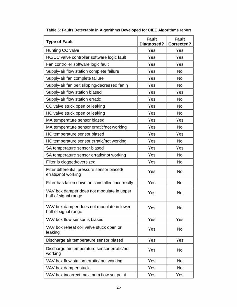
25

Table 5: Faults Detectable in Algorithms Developed for CIEE Algorithms report

Type of Fault Fault Diagnosed?

Fault Corrected?

Hunting CC valve Yes Yes HC/CC valve controller software logic fault Yes Yes Fan controller software logic fault Yes Yes Supply-air flow station complete failure Yes No Supply-air fan complete failure Yes No Supply-air fan belt slipping/decreased fan η Yes No Supply-air flow station biased Yes Yes Supply-air flow station erratic Yes No CC valve stuck open or leaking Yes No HC valve stuck open or leaking Yes No MA temperature sensor biased Yes Yes MA temperature sensor erratic/not working Yes No HC temperature sensor biased Yes Yes HC temperature sensor erratic/not working Yes No SA temperature sensor biased Yes Yes SA temperature sensor erratic/not working Yes No Filter is clogged/oversized Yes No

Filter differential pressure sensor biased/ erratic/not working

Yes No

Filter has fallen down or is installed incorrectly Yes No

VAV box damper does not modulate in upper half of signal range

Yes No

VAV box damper does not modulate in lower half of signal range

Yes No

VAV box flow sensor is biased Yes Yes

VAV box reheat coil valve stuck open or leaking

Yes No

Discharge air temperature sensor biased Yes Yes

Discharge air temperature sensor erratic/not working

Yes No

VAV box flow station erratic/ not working Yes No VAV box damper stuck Yes No VAV box incorrect maximum flow set point Yes Yes

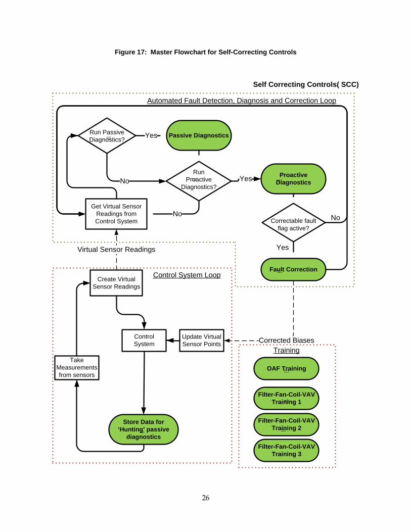
26

Figure 17: Master Flowchart for Self-Correcting Controls

Self Correcting Controls( SCC)

Run Passive Diagnostics?

Passive Diagnostics

Run Proactive

Diagnostics?No

Yes

No

Create Virtual Sensor Readings

Control System

Store Data for ‘Hunting’ passive

diagnostics

Proactive Diagnostics

Correctable fault flag active?

Fault Correction

Yes

No

Yes

Control System Loop

Update Virtual Sensor Points Corrected Biases

Get Virtual Sensor Readings from Control System

Virtual Sensor Readings

Automated Fault Detection, Diagnosis and Correction Loop

Take Measurements from sensors

OAF Training

Filter-Fan-Coil-VAV Training 1

Filter-Fan-Coil-VAV Training 2

Training

Filter-Fan-Coil-VAV Training 3

27

correcting controls process, there are additional steps in the process. The actual sensor measurements are input to virtual sensors, which generate corrected sensor values (when warranted). The corrected virtual values are then used by the control algorithms in place of erroneous sensor readings so that the controller sends the correct actuation signal to the actuator. From the standpoint of control, these virtual sensor readings replace the actual readings.

A green dotted line in Figure 17 encloses a separate process that executes simultaneously with the control system loop. This process is the automated fault detection, diagnostics, and correction loop (AFDDC). This process takes in sensor data from the virtual sensor points as well as control code information from the control system and continuously monitors those values for signs of faults.

As long as no faults are detected, the system runs through a sub-loop within this process that periodically checks for faults. The process of checking for faults is called Passive Diagnostics because faults are detected through passive, observation monitoring only, without affecting the control process.

When a fault is detected by the passive diagnostics, a process called Proactive Diagnostics is initiated. The proactive process diagnoses (or isolates) the fault. For example, passive diagnostics may detect that a set of sensors is displaying readings that are inconsistent with one another based on the physical relationships among the measured variables. Proactive diagnostics determine which, if any of the sensors, is reading improperly, or if the detected inconsistency might be caused by something like stuck dampers or leaking valves that produce the unexpected (abnormal) measured conditions. Proactive diagnostics involve taking control of the system away from its ordinary automatic operation and placing it into alternative states controlled by the AFDDC software. The AFDDC software places the system into specific conditions that enable isolation of the fault to a specific component (or cause). The proactive diagnostics can run automatically, immediately upon fault detection, can be scheduled to run at specific times, or can be run manually, when it is convenient for the building operator or occupants.

Once the fault has been successfully diagnosed, the AFDDC Fault Correction process starts, wherein the specific component is recalibrated so that its fault can be automatically accounted for by the control system via the creation of a new virtual sensor point. This is only possible, however, for “soft faults” or faults that exist in automatically correctable sensors or in the control code itself. The criteria for a sensor being automatically correctable varies, but generally involves having a working sensor available somewhere else in the system or a model that can be used along with correct measurements of other conditions in the physical process to infer the correct value that the faulty sensor would provide if it were working properly.

Another dotted line in Figure 17 encloses a set of Training processes. Many of the fault detection algorithms rely on models of the physical system behavior under normal operation. Because each system is inherently different, these models are empirically in an initial training process that could be part of the system’s commissioning. In training, the system’s normal (fault-free) operation is empirically and quantitatively characterized.

28

Training Four training algorithms are grouped under the set of training processes shown in Figure 17. The first one, titled “OAF Training” is used for detecting mixing-box faults, and is described in Fernandez et al. (2009b). The others are training algorithms for the filter/fan/coil section of the air handler of the VAV system and are described in detail in Fernandez et al. (2009a).

The “Filter/Fan/Coil/VAV Training 1” process, referred to subsequently as Training 1, develops empirical relationships between the normal supply-air flow rate (VS) and two parameters: 1) USF, the fan control signal, which is a voltage or current signal sent to the fan and is normalized to a range of 0-100% and 2) Udamp, the normalized control signal for the outdoor-air damper. The variable Udamp determines the outdoor-air damper position and, as a result, VS, given a value of the fan speed. While VAV dampers individually can affect air-flow resistance, all the dampers in the VAV boxes served by a specific air handler are typically controlled together to maintain the supply-air static pressure at a fixed value (its set point). This training algorithm fits the collected data to a two-factor polynomial regression equation.

Training 2 develops two empirical relationships. The first relates the normal temperature rise of the air as it passes across the fan (from fan motor heat rejection) as a function of VS. Measurements of the temperature increase are taken at discrete values of the fan speed over its full range, and are stored as a lookup table. Temperature increases from the fan for values of VS between the measured values of the table are determined by linearly interpolating. The second relates the normal filter pressure drop to VS, again based on measurements of the pressure drop across the filter at selected values of VS over its full range. The measured results are stored in a lookup table and values of pressure drop for intermediate values of VS are obtained by linear interpolation.

Training 3 develops an empirical relationship between ΔTSM, which is the difference between the supply-air temperature and the mixed-air temperature, and two variables, VS and the control signal for the chilled-water valve of the cooling coil, UCC. Measurements are made and a polynomial curve fit is used to establish the relationship.

Passive Diagnostics Figure 18 shows the main passive diagnostics process for the filter/fan/coil and VAV box sections. The passive diagnostics process is serial, executing a set of algorithms sequentially until a fault is found, at which point the Passive Diagnostics process terminates and the proactive diagnostics process begins (according to how it is scheduled) or until all of the algorithms have passed without detection of a fault.

Key information can be obtained from the passive diagnostics about the nature of the fault that dictates which proactive tests are necessary to isolate and diagnose the fault. The specific passive diagnostic rule that detects the symptom of a fault provides one clue. Other clues can sometimes be obtained from the sequence of passive diagnostic tests. For example, if Fault 1 always causes both symptom A and symptom B, and Faults 2 and 3 cause symptom B, but not symptom A, then if the occurrence of symptom A is checked before the presence of symptom B and found not to be present, Fault 1 can be ruled out when symptom B is present. This type of logic is employed in the passive diagnostic algorithms through use of a set of “flags.” These

29

Figure 18: Passive Diagnostics for Filter/Fan/Coil/VAV Boxes

Check Fan and Coil Signals

VAV Box Passive Diagnostics

Passive Diagnostics: Filter-Coil-Fan-VAV Control Signal

Logic

Check Supply Air Temperature

Fault Detected?

No

Main Program:Run Proactive

Diagnostics?

Yes

Passive Diagnostics: Fault

Detected?

No

Setpoint Maintenance

No

Fault Detected?

No

Fault Detected?

Fault Detected?

No

Check Filter Pressure Drop No

Yes

Yes

Check for Hunting Cooling Coil

Yes

30

numbered flags are raised at specific points in the passive diagnostic process when faults are detected. The flags then direct the flow of proactive diagnostic tests so that only the remaining tests necessary to diagnose the observed symptom are performed.

Descriptions of the individual algorithms run sequentially in the passive diagnostics follow [see also Fernandez et al. (2011)].

Check for Hunting Cooling Coil – This algorithm checks that the cooling coil valve is not “hunting.” A hunting actuator is one that oscillates around the position it is seeking. Poorly set values of control constants in the proportional-integral (PI) or proportional-integral-derivative (PID) controller for the cooling coil valve actuator can cause this. The algorithm for checking for hunting uses a database of past cooling coil command signals to detect whether hunting is taking place. No proactive diagnostics are needed to detect this fault.

Control System Logic – This algorithm checks to ensure that flow through the air-handler heating coil and cooling coil do not occur at the same time. It checks whether both the heating and cooling coils are properly off when the system is economizing with the outdoor-air damper signal Udamp < 100% open and that the heating coil is off when the system is economizing at Udamp =100%. Violation of these faults indicates incorrect control algorithms for the air-handler damper system, and can be automatically corrected with a correct algorithm upon detection; no proactive diagnostics are needed to isolate the fault.

Check Supply-air Temperature – This algorithm uses training data from Training 2 to determine if the observed fan heat gain matches the training closely enough. This is done by monitoring the difference between the supply-air temperature and cooling coil inlet temperature. If the heating and cooling coils are off, the allowable supply-air temperature is bound on both sides by temperature tolerances to the temperatures expected from Training 2. If one of the coils is commanded on, the allowable supply-air temperature is only bounded on one side, i.e., if the cooling coil is on, the algorithm checks to make sure the supply-air temperature sensor is not reading higher than the cooling coil inlet temperature plus the fan temperature rise and the temperature tolerances.

Set Point Maintenance - This algorithm checks whether both the supply-air temperature and supply-air static pressure are correctly within acceptable ranges of their set points. If the supply-air temperature cannot maintain its set point, but the coils are not being commanded on, or if the supply-air static pressure cannot maintain its set point, but the fan is not being commanded on, this indicates a control software (or algorithm) fault that is automatically correctable. Otherwise, these conditions might indicate a fault somewhere else in the system.

Check Fan and Coil Signals – This algorithm uses the regression equations from Training 1 and Training 3 to determine if a) the current value of the coil coil control signal, UCC, is providing the expected degree of cooling, as measured by the difference between the supply-air and mixed-air temperatures, given the current supply-air flow rate and b) if the current value of the supply-fan control signal, USF, is providing the expected supply-air flow rate, given the current outdoor-air damper position. Readings that are outside of acceptable ranges could indicate a number of different faults.

VAV Box – This algorithm checks the sensor measurements from the VAV boxes for symptoms of faults. First, for each VAV box whose reheat coil has been off for at least 10 minutes and whose damper is at least partially open, it checks whether the VAV-box discharge-air

31

temperature is correctly within specified tolerances of the supply-air temperature set point. Next, it checks whether the room temperature is within the proper range of the heating and cooling set-point temperatures. This condition is acceptable, especially given the time delay between detecting that the room temperature differs from its set point by an unacceptable amount and subsequently returning the room temperature to the set point. If the temperatures are outside acceptable tolerance of the set points, the algorithm also checks whether the VAV- box flow meter indicates a box air-flow rate correctly above its minimum set point, and when heating is required, that the reheat coil for the VAV box is commanded on. If these conditions are violated a fault is present.

Check Filter Pressure Drop- This algorithm uses Training 2 data to determine whether the fan’s differential pressure sensor is reading within acceptable ranges. If the pressure drop is too high, a clogged filter that needs to be replaced could be indicated. If it is too low, the filter could be missing, have fallen down out of its frame, or have been improperly installed. Low filter pressure drop could also indicate that the sensor itself is faulty or that a fan fault exists. As with most other instances of fault detection, further proactive diagnostics are needed to isolate the specific fault.

Proactive Diagnostics Proactive diagnostics begin subsequent (either immediately, or scheduled later) to the detection of a passive fault that cannot be automatically isolated and corrected. Figure 19 shows the overall process of proactive diagnostics for the filter-fan-coil-VAV section. Unlike the passive diagnostics, there is more management of the direction of logical flow through this proactive diagnostics process to efficiently schedule the tests - eliminating unnecessary testing.

Proactive diagnostics always start with Check Fan. A fan that is completely stuck or not functioning could potentially lead to all of the undiagnosed faults detected in the passive diagnosis. Thus, verifying that the fan is, in fact, working is critical. This test starts by checking that the measured supply-air flow rate matches its baseline values for full, medium and off fan speeds established during training. If the values do not adequately match, the flow rate is verified to increase as the supply-fan command is increased. A failure to meet this criterion could indicate either a broken/unresponsive fan or a supply-air flow station that is not working. A further check is used to differentiate these two potential causes. The filter differential pressure is checked to verify that it increases as the fan control signal is increased. If it too, does not change appreciably, the fault is associated with a broken supply fan. If the differential pressure does change, it implicates a complete failure of the supply-fan air-flow station.

If, on the other hand, the measured flow rate does increase as the fan control signal is increased, either the fan or the flow station has dropped out of calibration compared to its training baseline, but is still operating. A further test in this case checks for two symptoms that may exist if the problem is a decrease in fan efficiency (i.e., fan producing decreased mechanical output for a given control signal – one cause is a slipping fan belt). If this were the only fault, the deviation from training flow rates would be much greater at a full fan control signal 100% compared to the deviation when the control signal is zero (i.e., off). The filter pressure drop would also be lower for each specific fan control signal than the pressure drop during training,

32

Figure 19: Proactive Diagnostics for Filter/Fan/Coil and VAV Box Sections: Main Flowchart

Proactive Diagnostics: Filter-Coil-Fan-VAV

Check Fan

Fault Diagnosed?

Proactive Flag A?

Passive Diagnostics: Fault

Detected?

No

Check Temperature Sensors and Coils

Fault Diagnosed?

Proactive Flag G?

Proactive Flag C,F?

No

Check Filter

VAV Box: Check all Dampers

VAV Box: Temp Sensors and Reheat

Valves

VAV Box: VAV Box Flow Sensor

VAV Box: Check Max Flow Setpoint

Fault Diagnosed?

Fault Diagnosed?

Fault Diagnoesd?

No

No

No

Yes

Fault Diagnosed?

Proactive Flag B,D?

Proactive Flag C?

No

Fault: Static Pressure Sensor

Yes

Proactive Diagnostics:

Inconclusive Fault- Clear Flags

No

Yes

Proactive Diagnostics:

Inconclusive Fault- Clear Flags

Main Program:Run

Fault Correction?

Yes

Yes

Yes

Yes

Yes

No

Yes

Yes

Yes

No

No

33

because the fan is not able to drive as much flow and, therefore, not able to establish as strong a pressure drop across the filter. The satisfaction of these two criteria automatically implicates a faulty fan. A partially clogged filter muddies the analysis, however, because clogging may act to increase the filter pressure drop. The assumption here is, however, that a clogged filter alone will not decrease the fan air flow rate sufficiently compared to training baseline values to bypass this entire set of algorithms. If however, the partially clogged filter occurs in conjunction with a slipping fan belt, for instance, it may hinder the detection of the slipping fan belt using this process (flowchart) alone. Thus, a somewhat redundant algorithm is used to distinguish between these different situations. This algorithm compares the measured supply-air flow rate against a few the individual VAV box measured flow rates. This requires closing all of the VAV dampers but one and measuring the flow rate at the fully open damper. Normal leakage through the network of closed dampers and ductwork needs to be accounted for (which is the purpose of the leakage flow testing performed in training). This training-based leakage flow is subtracted from the measured supply- air flow rate before comparison to the VAV box measured flow rate. If the two flow rates roughly match, the result implicates decreased efficiency of the supply fan, whereas if the values do not match adequately, this implicates a working, but faulty, supply-air flow station.

If no faults are found in the fan or flow station, the measured flow rate should be reasonably close to the baseline (training) value, and selected proactive tests can then be scheduled according to clues from the passive diagnostics. If Proactive Flag A,B, or D is active (these flags are raised in response to several conditions in the passive diagnostics; see Fernandez et al. 2011), the Check Temperature Sensors and Coils process is performed. A fault can be traced to one of the three air-handler temperature sensors (mixed air, cooling-coil inlet air, or supply air) or to a leaking heating or cooling coil. Fault isolation is accomplished by setting the heating and cooling coil control signals to zero and monitoring the differences between the values of the three mixing-box temperature sensors at three fan speeds: low, medium, and full. Much of the differentiation relies on the temperature difference across a leaking heating or cooling coil decreasing with increased air-flow rate (even as the total heating or cooling imparted to the air stream increases). If the temperature change across the coils does not decrease with increasing flow rate, the fault is almost certainly with one of the temperature sensors, which can then be isolated by checking the three sensor readings against each other, accounting for fan temperature rise.

The Check Filter process follows next. It runs when a flag for a fault occurs in the filter check during the passive diagnostics (and no faults have been isolated thus far). The algorithm isolates physical filter faults from pressure-drop sensor faults by setting the supply fan to zero and checking the measured pressure drop. If it is non-zero, the fault is isolated to the pressure sensor. If the pressure drop reads zero with the fan off, the fault is isolated to either a clogged filter, if the pressure drop was higher than the training value when the fault was detected, or to a missing, fallen or improperly installed filter, if the pressure drop was lower than the training value when the fault was detected.

After the Check Filter process is completed, all potential faults in the air-handler filter-fan-coil section have been considered, leaving faults in the VAV boxes undiagnosed. When a flag is raised in the passive diagnosis that indicates the possibility of a VAV-box fault, four VAV box tests is performed sequentially until a fault is isolated.

34

The first test for VAV boxes, VAV Box: Check All Dampers, uses sensed data for a range of fan speeds for all VAV boxes to isolate either faulty dampers or faulty VAV-box flow sensors in any of the VAV boxes. Stuck dampers and completely non-functional VAV-box flow stations are indistinguishable at this point. If one of these faults exists, a new flag is raised, and an additional test is used to isolate the fault.

If no faults are found in the VAV-box flow stations and there is a flag for a specific faulty VAV box from the passive diagnostics, the next algorithm, VAV Temperature Sensors and Reheat Valves runs. This process differentiates between faulty (leaking or stuck) VAV-box reheat valves and faulty VAV discharge-temperature sensors by checking for a coil heat-gain signature (decreasing temperature difference across the reheat coil at increasing air-flow rate). If this signature is present, the fault is traced to a leaking or stuck open reheat valve. If instead the temperature difference across the reheat coil (difference between the VAV-box discharge air temperature and the temperature of air entering the VAV box) is unchanged or increases , the fault is traced to the discharge-air temperature sensor itself. If the discharge-air temperature remains constant at all reheat coil command signals, the fault is traced to a reheat coil valve that is stuck closed. Otherwise, no faults related to VAV box temperature sensors or coils can be diagnosed.

If no faults have yet been diagnosed in the VAV box, the VAV Box Flow Sensor process is used to isolate a faulty VAV-box flow-rate sensor. In this process, the VAV-box flow rate is checked against the supply-air flow rate at low fan speeds, when all other VAV-box dampers are completely closed. The assumption here is that at low fan speeds there will be negligible leakage flow through the other dampers. This assumption needs to be verified. If it is not a valid assumption, further data collection (training) may be required to quantify low-fan speed VAV system leakage (in addition to the full-speed leakage already performed). If the VAV-box flow rate does not match the supply-air flow rate, the result indicates a faulty VAV flow meter. If the readings match and Flag H is active, the fault is traced to a stuck VAV-box damper.

If no faults are detected after completion of the VAV Temperature Sensors and Reheat Valves process, one final VAV diagnostic test called VAV Box Maximum Flow Rate Set Point is performed. This process tests whether the VAV box can meet its maximum flow-rate set point. At this point, all other components of the VAV box have been verified to be working properly, so this test should represent a conclusive test of the VAV box’s capability. If it passes this test, the detection of a fault in the passive diagnostics may have been an aberration, and the diagnostics should be reset, the system returned to normal operation, and the passive diagnostics instigated once more. There is one exception to this, however. If the supply-air pressure sensor could not meet its set point (leading to Proactive Flag C), and all other components and processes are determined function properly within the proactive diagnostics, the supply-air pressure sensor is deemed to be faulty by the process of elimination. There is no other way to test this sensor for a VAV system as instrumented.

Fault Correction Figure 20 shows the overall process flowchart for automatic fault correction. Automatic correction of diagnosed soft faults occurs subsequent to their diagnosis in the fault correction process. Two classes of soft faults (software errors and hunting) are corrected automatically as

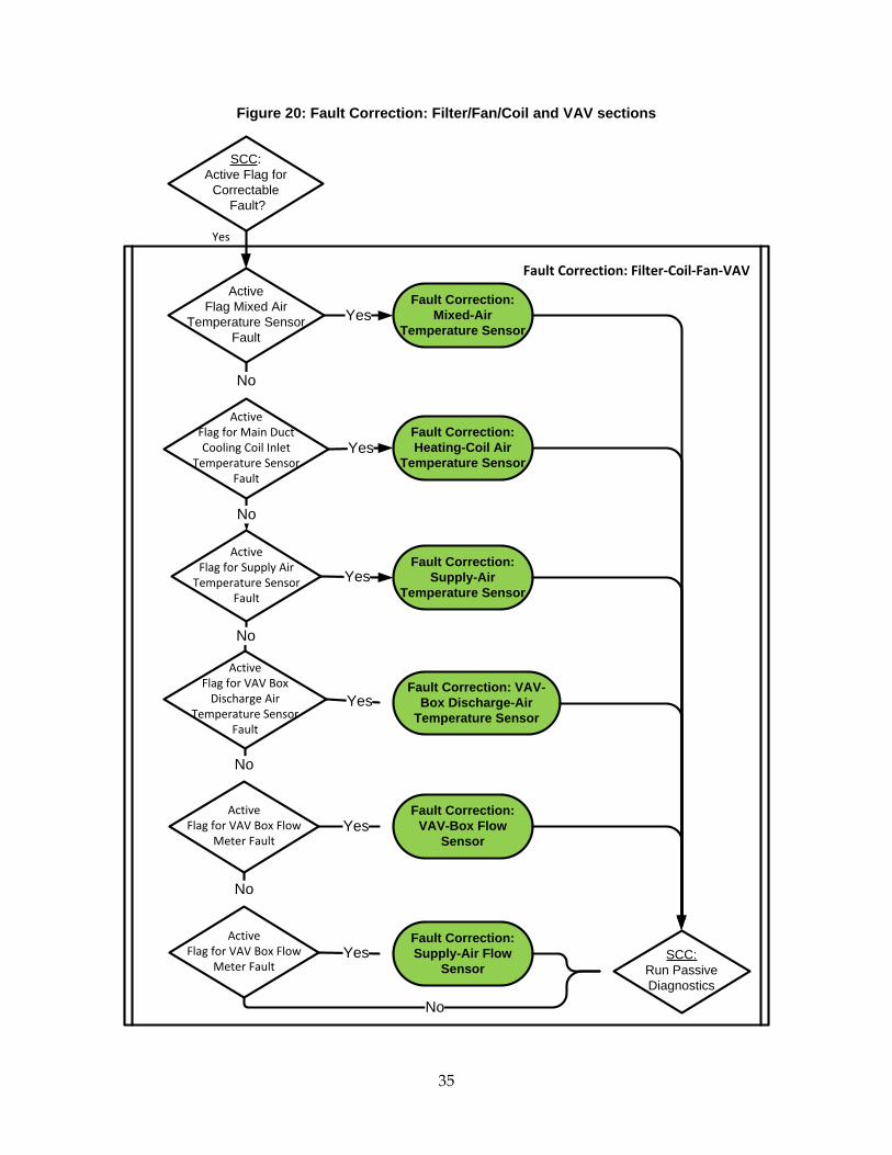
35

Figure 20: Fault Correction: Filter/Fan/Coil and VAV sections

Active Flag Mixed Air

Temperature Sensor Fault

Fault Correction: Filter-Coil-Fan-VAV

SCC: Active Flag for

Correctable Fault?

Yes

Fault Correction: Mixed-Air

Temperature SensorYes

SCC: Run Passive Diagnostics

Active Flag for Main Duct Cooling Coil Inlet

Temperature Sensor Fault

Fault Correction: Heating-Coil Air

Temperature SensorYes

No

No

Active Flag for Supply Air

Temperature Sensor Fault

Active Flag for VAV Box

Discharge Air Temperature Sensor

Fault

Active Flag for VAV Box Flow

Meter Fault

Active Flag for VAV Box Flow

Meter Fault

No

No

No

No

Fault Correction: Supply-Air

Temperature Sensor

Fault Correction: VAV-Box Discharge-Air

Temperature Sensor

Fault Correction: VAV-Box Flow

Sensor

Fault Correction: Supply-Air Flow

Sensor

Yes

Yes

Yes

Yes

36

they are detected in the passive diagnostics. This leaves one class of soft faults (sensor biases) that need to be corrected after the proactive diagnostics. There are four types of sensors and two types of flow-rate sensors that can be corrected using the processes presented here. The correction process involves calibrating the faulty sensor against a working sensor in the same airstream. First, however, the behavior of the faulty sensor is checked to determine whether its output is nearly constant over time compared to the working sensor against which it will be calibrated. If the difference is constant, this indicates a bias that can be readily determined and corrected by subtracting a constant value for the incorrect measured value in a virtual sensor placed in the control system loop. If it is not constant, correction of the fault will require a more complex behavioral characterization not developed yet, or the sensor may behave erratically or have failed in some way, both of which require that the faulty sensor be replaced.

The mixed-air and cooling coil inlet air-temperature sensor outputs can be recalibrated directly from the other, unbiased sensor. Likewise the supply-air and any VAV-box air-temperature sensor can be recalibrated directly by using the other. The supply-air flow-rate sensor and any of the individual VAV-box air-flow sensors can be recalibrated to the other, unbiased sensor, but account must be made for air-flow leakage between the measurement points (i.e., using a, albeit simple, model). Most properly working dampers still leak slightly when they are completely closed, so it may not be possible to entirely isolate the flow into any one damper. Therefore, a leakage flow is characterized during Training 2 that can be used in this fault correction. The leakage flow rate is the difference between the supply-air flow rate and the flow rate at any one VAV damper that is open while the rest are closed.

37

CHAPTER 3: Implementation and Testing The algorithms developed to detect, diagnose, and correct faults in VAV systems were implemented for laboratory testing by coding them into a programming package that interacts with Factory Plant Management Interface (FPMI) software. In this project, FPMI is used as a human/machine interface (HMI). FPMI is a web-deployed front-end to the Object Linking and Embedding for Process Control (OPC) server and Structured Query Language (SQL) Database. Using the FPMI client interface, users can monitor live data, specify the control variables and sensor paths, and instigate diagnostic and correction tests, including the instigation of faults. Using a database server, the test data and control variables can be stored automatically. In this way, the algorithms we develop are implemented in software code that is used to control the physical system that has been constructed as a test facility for investigating the performance of the algorithms for automated fault detection and correction.

Description of the Test Facility Section 3 of Fernandez et al. (2009b) provides a description of the laboratory facility used to test the VAV system algorithms. In brief, the system is composed of a chilled water loop that provides chilled water to the coiling coil of an air handler. The air handler draws outdoor air from the environment and mixes it with return air from the room the air handler is located in. An electric heater maintains this room at a temperature set point. The mixed air flows through the chilled water coil, then through a fan and a flow-rate sensor. The test facility has been updated for this project to include four pressure-independent VAV boxes. From the discharge of air handler, where the flow rate sensor is located, the air stream branches to each of the VAV boxes. Each VAV box includes a damper, discharge-air temperature sensor, and a flow meter.

Implementation of Algorithms Priorities were set for implementation of the algorithms in software code to ensure compatibility with the available project budget. The goals of this prioritization were the following:

• Code a set of algorithms that enabled testing the entire process (fault detection, diagnostics, and correction), albeit for a limited number of faults

• Focus on automatically-correctable, or soft faults, as opposed to hard faults

• Include faults that had many diagnostic pathways so that diagnosis of the correct fault could be verified

• Include all of the training algorithms, because data from these training tests is a valuable tool for future refinement of the algorithms.

With these goals in mind, a set of algorithms was selected that enabled implementation of faults in the supply-air temperature sensor and the supply-air flow meter, while differentiating these faults from those originating from the cooling-coil valve, the fan, other temperature sensors, and the VAV-box flow sensors.

38

The algorithms developed and the subset implemented in software are identified in Table 6.

Table 6: Algorithms Developed and Implemented (Coded) for Testing

Algorithms Developed Algorithms Coded

Training Algorithms Filter-fan-coil-VAV section, training algorithm 1: expected fan signal

Filter-fan-coil section of VAV air-handler, training algorithm 2: single-factor variables

Filter-fan-coil-VAV section, training algorithm 3: expected cooling coil valve signal

Passive Diagnostics Algorithm for Control System Loop Control system loop: store data for hunting passive diagnostics

Passive Diagnostics Algorithms Automatic detection and correction of hunting Control system logic Check supply-air temperature Set-point maintenance Check fan and coil signals Check filter pressure drop

Proactive Diagnostics Algorithms Check fan Check supply-air flow sensor Temperature sensors and coil valves Check filter VAV: Check all dampers

VAV: Temperature sensors and reheat valves

VAV: VAV-box flow sensors

VAV: VAV-box maximum flow rate set point

Fault Correction Algorithms Mixed-air temperature sensor Cooling-coil inlet-air temperature sensor Supply-air temperature sensor Supply-air flow-rate sensor Control system logic 1 Control system logic 2 VAV discharge-air temperature sensor

VAV flow sensor

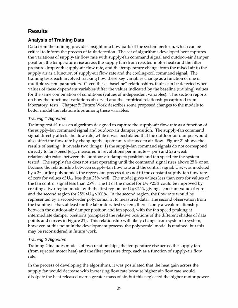
39

Results Analysis of Training Data Data from the training provides insight into how parts of the system perform, which can be critical to inform the process of fault detection. The set of algorithms developed here captures the variations of supply-air flow rate with supply-fan command signal and outdoor-air damper position, the temperature rise across the supply fan (from rejected motor heat) and the filter pressure drop with supply-air flow rate, and the temperature change from the mixed air to the supply air as a function of supply-air flow rate and the cooling-coil command signal. The training tests each involved tracking how these key variables change as a function of one or multiple system parameters. Given these “baseline” relationships, faults can be detected when values of these dependent variables differ the values indicated by the baseline (training) values for the same combination of conditions (values of independent variables). This section reports on how the functional variations observed and the empirical relationships captured from laboratory tests. Chapter 5: Future Work describes some proposed changes to the models to better model the relationships among these variables.

Training 1 Algorithm Training test #1 uses an algorithm designed to capture the supply-air flow rate as a function of the supply-fan command signal and outdoor-air damper position. The supply-fan command signal directly affects the flow rate, while it was postulated that the outdoor-air damper would also affect the flow rate by changing the upstream resistance to air-flow. Figure 21 shows the results of testing. It reveals two things: 1) the supply-fan command signals do not correspond directly to fan speed (e.g., measured in revolutions per minute—rpm) and 2) a weak relationship exists between the outdoor-air dampers position and fan speed for the system tested. The supply fan does not start operating until the command signal rises above 25% or so. Because the relationship between supply-fan flow rate and the control signal, USF, was modeled by a 2nd order polynomial, the regression process does not fit the constant supply-fan flow rate of zero for values of USF less than 25% well. The model gives values less than zero for values of the fan control signal less than 25%. The fit of the model for USF<25% could be improved by creating a two-region model with the first region for USF<25% giving a constant value of zero and the second region for 25%<USF≤100%. In the second region, the flow rate would be represented by a second-order polynomial fit to measured data. The second observation from the training is that, at least for the laboratory test system, there is only a weak relationship between the outdoor-air damper position and fan speed, with the fan speed peaking at intermediate damper positions (compared the relative positions of the different shades of data points and curves in Figure 21). This relationship will likely change from system to system, however, at this point in the development process, the polynomial model is retained, but this may be reconsidered in future work.

Training 2 Algorithm Training 2 includes models of two relationships, the temperature rise across the supply fan (from rejected motor heat) and the filter pressure drop, each as a function of supply-air flow rate.

In the process of developing the algorithms, it was postulated that the heat gain across the supply fan would decrease with increasing flow rate because higher air-flow rate would dissipate the heat released over a greater mass of air, but this neglected the higher motor power

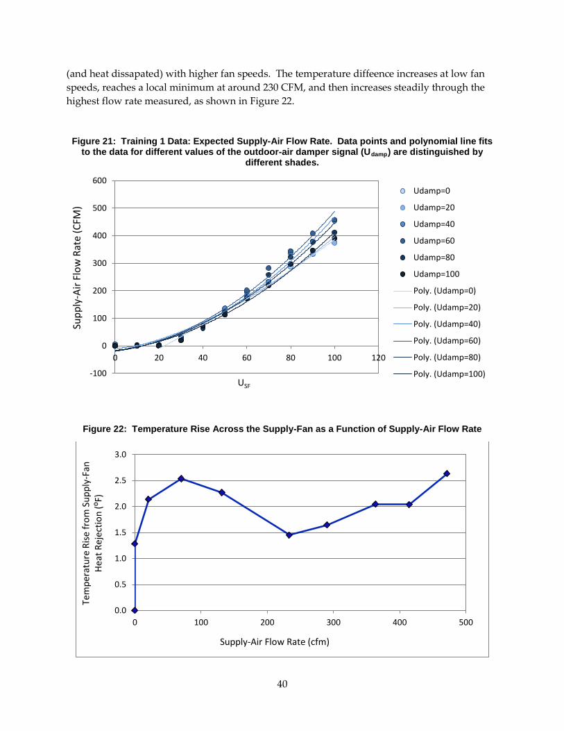
40

(and heat dissapated) with higher fan speeds. The temperature diffeence increases at low fan speeds, reaches a local minimum at around 230 CFM, and then increases steadily through the highest flow rate measured, as shown in Figure 22.

Figure 21: Training 1 Data: Expected Supply-Air Flow Rate. Data points and polynomial line fits to the data for different values of the outdoor-air damper signal (Udamp) are distinguished by

different shades.

Figure 22: Temperature Rise Across the Supply-Fan as a Function of Supply-Air Flow Rate

-100

0

100

200

300

400

500

600

0 20 40 60 80 100 120

Udamp=0

Udamp=20

Udamp=40

Udamp=60

Udamp=80

Udamp=100

Poly. (Udamp=0)

Poly. (Udamp=20)

Poly. (Udamp=40)

Poly. (Udamp=60)

Poly. (Udamp=80)

Poly. (Udamp=100)

Supp

ly-A

ir Fl

ow R

ate

(CFM

)

USF

0.0

0.5

1.0

1.5

2.0

2.5

3.0

0 100 200 300 400 500

Supply-Air Flow Rate (cfm)

Tem

pera

ture

Rise

from

Sup

ply-

Fan

He

at R

ejec

tion

(⁰F)

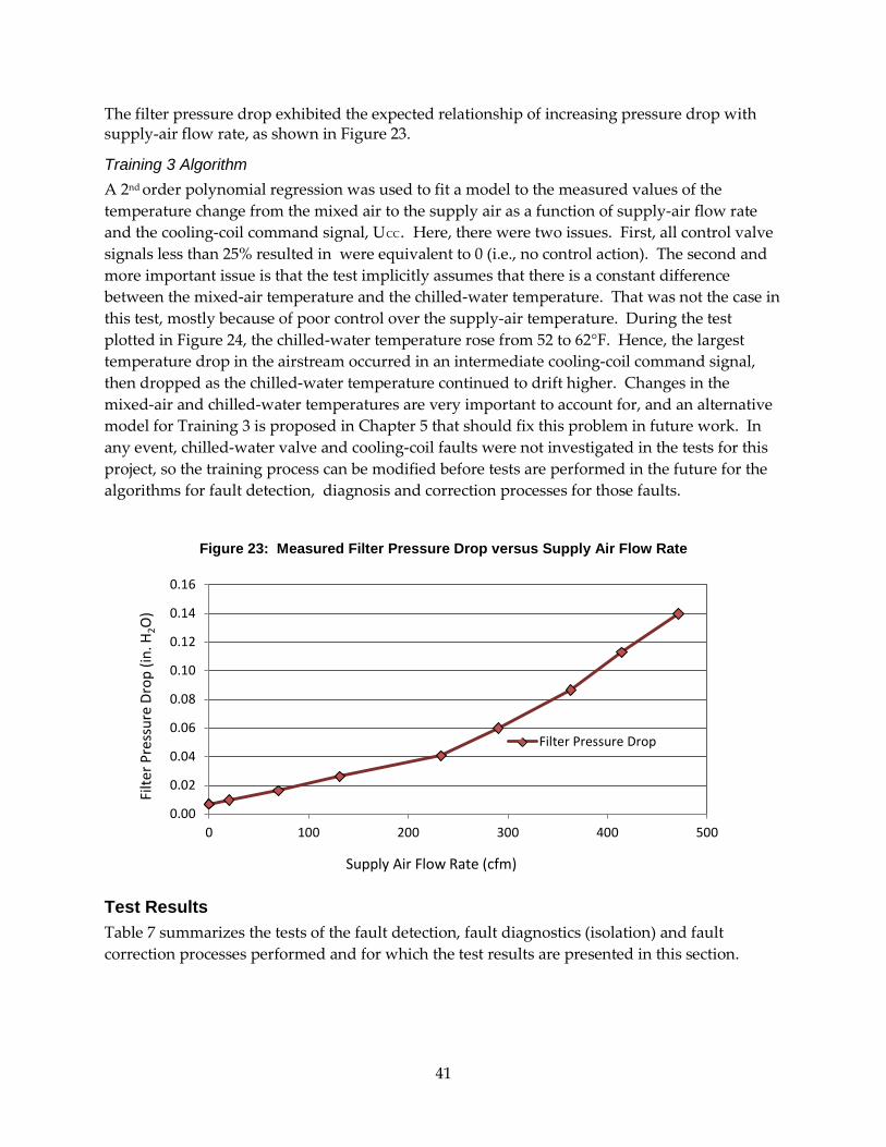
41

The filter pressure drop exhibited the expected relationship of increasing pressure drop with supply-air flow rate, as shown in Figure 23.

Training 3 Algorithm A 2nd order polynomial regression was used to fit a model to the measured values of the temperature change from the mixed air to the supply air as a function of supply-air flow rate and the cooling-coil command signal, UCC. Here, there were two issues. First, all control valve signals less than 25% resulted in were equivalent to 0 (i.e., no control action). The second and more important issue is that the test implicitly assumes that there is a constant difference between the mixed-air temperature and the chilled-water temperature. That was not the case in this test, mostly because of poor control over the supply-air temperature. During the test plotted in Figure 24, the chilled-water temperature rose from 52 to 62°F. Hence, the largest temperature drop in the airstream occurred in an intermediate cooling-coil command signal, then dropped as the chilled-water temperature continued to drift higher. Changes in the mixed-air and chilled-water temperatures are very important to account for, and an alternative model for Training 3 is proposed in Chapter 5 that should fix this problem in future work. In any event, chilled-water valve and cooling-coil faults were not investigated in the tests for this project, so the training process can be modified before tests are performed in the future for the algorithms for fault detection, diagnosis and correction processes for those faults.

Figure 23: Measured Filter Pressure Drop versus Supply Air Flow Rate

Test Results Table 7 summarizes the tests of the fault detection, fault diagnostics (isolation) and fault correction processes performed and for which the test results are presented in this section.

0.00

0.02

0.04

0.06

0.08

0.10

0.12

0.14

0.16

0 100 200 300 400 500

Filter Pressure Drop

Filte

r Pre

ssur

e Dr

op (i

n. H

2O)

Supply Air Flow Rate (cfm)

42

Figure 24: Difference Between the Mixed-air and Supply-air Temperatures Plotted against Supply-Air Flow Rate for Values of the Cooling-Coil Control Signal (UCC) from 0 and 100%.

Table 7: Summary of Tests Performed and Primary results. Check marks identify tests that were performed with successful results.

Test Number and Fault Description

Fault Severity

Key Tolerances*

Passive Diagnostics

Proactive Diagnostics

Fault Correction

1. Supply-air Temperature Sensor Bias

+5⁰F Ttol=2⁰F

USF,tol=10 Inconclusive

2. Supply-air Temperature Sensor Bias

+5⁰F Ttol=1⁰F

USF,tol=10 Corrected Bias of +4.1⁰F

3. Supply-air Temperature Sensor Bias

+8⁰F Ttol=2⁰F

USF,tol=10 Corrected Bias of +6.6⁰F

UCC = 0

UCC = 10

UCC = 20

UCC = 30

UCC = 40

UCC = 50

UCC = 60

UCC = 70

UCC = 80

UCC = 90

UCC = 100

Supply-Air Flow Rate (CFM)

43

4. Supply-air Flow Rate Bias

+265 cfm (20% of max flow)

Ttol=2⁰F

USF,tol =10 Concluded that the bias was erratic: replace sensor

5. Supply-air Flow Rate Bias

+265 cfm (20% of max flow)

Ttol=2⁰F

USF,tol =10 Corrected bias of 287.5 cfm

6. Supply-air Flow Rate Bias

+132 cfm (10% of max flow)

Ttol=2⁰F

USF,tol =10 Conclusion: Fan belt slipping or decrease in fan efficiency

*The subscript “tol” designates that the value given represents the tolerance for the variable that it subscripts.

In Test #1, a 5⁰F supply-air temperature sensor bias was instigated with a 2⁰F temperature sensor tolerances used in the algorithms. The supply-air temperature sensor biases are usually detected with the “Check supply-air temperature” algorithm. The fault is detected as a consequence of the heat gain across the fan exceeding the acceptable range of fan heat gain (at the current supply-air flow rate) during Training 2. The acceptable range is defined according to the tolerances of the temperature sensors. In this case, the test was performed with the algorithms using ±2⁰F tolerances applied to all temperature sensors (i.e, assuming that each temperature sensor has an uncertainty of ±2⁰F ). Because the air temperture increase caused by heat gain from the fan is calculated as the difference between the air temperture downstream of the fan and the the cooling coil inlet temperature (when the cooling coil is off; see Figure 1), the deviation in the temperature difference must exceed the expected training value by 4⁰F or more to conclude that the fault exists.

Figure 25 shows the time series of the deviations of the air temperature rise caused by fan heat rejection from its expected value based on the relationship found in Training 1. During the first several minutes of the test, there was no fault implemented, and the fan temperature rise was about 1⁰C lower than the equivalent training value. This period is labeled on the figure as point 1. At point 2, a fault is implemented by adding a 5⁰F bias to the supply-air temperature sensor output. This brings the air-temperature rise to just over 4⁰F, which is the threshold for detection of this fault. The fault is quickly detected at point 3, and proactive diagnostics are started (beginning of region in elipse labeled 4). During the proactive diagnostics, a series of tests is performed (see Fernandez et al. 2011) to isolate the fault as a supply-air temperature sensor fault (rather than being a bias in the mixed-air temperature sensor or a leaking heating coil, among other faults). A problem occurs during the fault isolation process. During the proactive diagnostic testing, at the specific point in the test where the supply-air temperature was

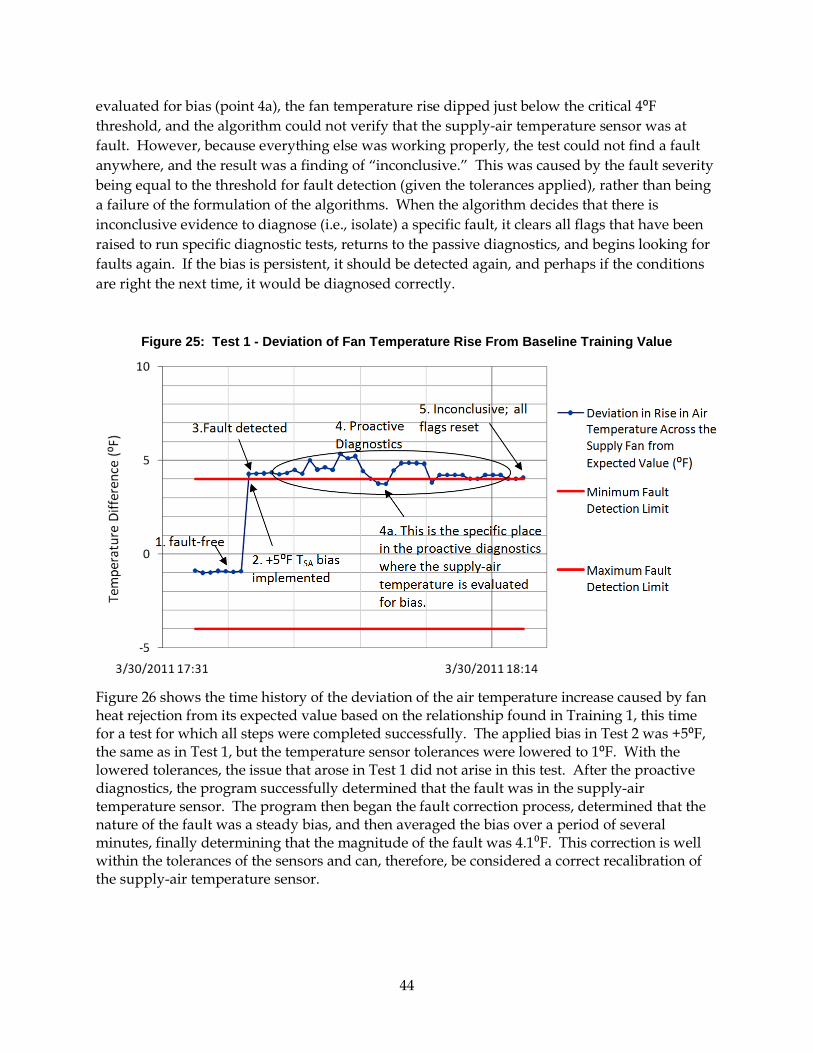
44

evaluated for bias (point 4a), the fan temperature rise dipped just below the critical 4⁰F threshold, and the algorithm could not verify that the supply-air temperature sensor was at fault. However, because everything else was working properly, the test could not find a fault anywhere, and the result was a finding of “inconclusive.” This was caused by the fault severity being equal to the threshold for fault detection (given the tolerances applied), rather than being a failure of the formulation of the algorithms. When the algorithm decides that there is inconclusive evidence to diagnose (i.e., isolate) a specific fault, it clears all flags that have been raised to run specific diagnostic tests, returns to the passive diagnostics, and begins looking for faults again. If the bias is persistent, it should be detected again, and perhaps if the conditions are right the next time, it would be diagnosed correctly.

Figure 25: Test 1 - Deviation of Fan Temperature Rise From Baseline Training Value

Figure 26 shows the time history of the deviation of the air temperature increase caused by fan heat rejection from its expected value based on the relationship found in Training 1, this time for a test for which all steps were completed successfully. The applied bias in Test 2 was +5⁰F, the same as in Test 1, but the temperature sensor tolerances were lowered to 1⁰F. With the lowered tolerances, the issue that arose in Test 1 did not arise in this test. After the proactive diagnostics, the program successfully determined that the fault was in the supply-air temperature sensor. The program then began the fault correction process, determined that the nature of the fault was a steady bias, and then averaged the bias over a period of several minutes, finally determining that the magnitude of the fault was 4.1⁰F. This correction is well within the tolerances of the sensors and can, therefore, be considered a correct recalibration of the supply-air temperature sensor.

45

Figure 26: Test 2 - Deviation of Fan Temperature Rise from Expected Training Value

Plotting the time series of the same variable (i.e., the deviation of the air temperature increase caused by fan heat rejection from its expected value) during Test 3 in Figure 27 shows the results of the same fault correction process, this time for a +8⁰F supply-air temperature sensor bias. This test illustrates that an increased severity (magnitude) of the fault has the same practical effect as lowering the tolerances for fault detection. If the tolerances were lowered too far, however, the rate of false fault detection would increase substantially. In Test 3, the fault was identified correctly as a supply-air bias fault with a magnitude of 6.63⁰F and corrected.

Tests 4 through 6 examined detection, diagnosis and correction of biases in the measurements by the supply-air flow-rate meter. Two levels of fault severity were tested, a bias of +10% of the full speed air-flow rate (132 cfm) and a bias of +20% of the full speed air-flow rate (265 cfm). Tests 4 and 5 were each at +20% severity.

The algorithms easily detected and isolated the Test 4 fault because the value of the supply fan control signal, USF, was well above the range of USF,cal [the expected value of USF obtained from the empirical relation between the normal supply-air flow rate (VS) and USF developed in Training 1]. As shown in Table 5, the tolerance for the supply-fan control signal USF,tol was set to 10. Therefore, USF must deviate from USF,cal by at least 10 for a bias fault to be detected. In Test 4, after detection of a fault, the proactive diagnostics successfully isolated the fault to the supply-air flow meter; however, the fault was incorrectly characterized as caused by an erratic sensor rather than a steady bias in the flow meter measurements.

During the fault correction process, the readings from the faulty sensor are monitored for a period of 15 minutes under controlled conditions to evaluate whether they are relatively constant. When a relatively constant bias persists for 15 minutes, the algorithm deems the fault condition a biased sensor, rather than acting erratic one.

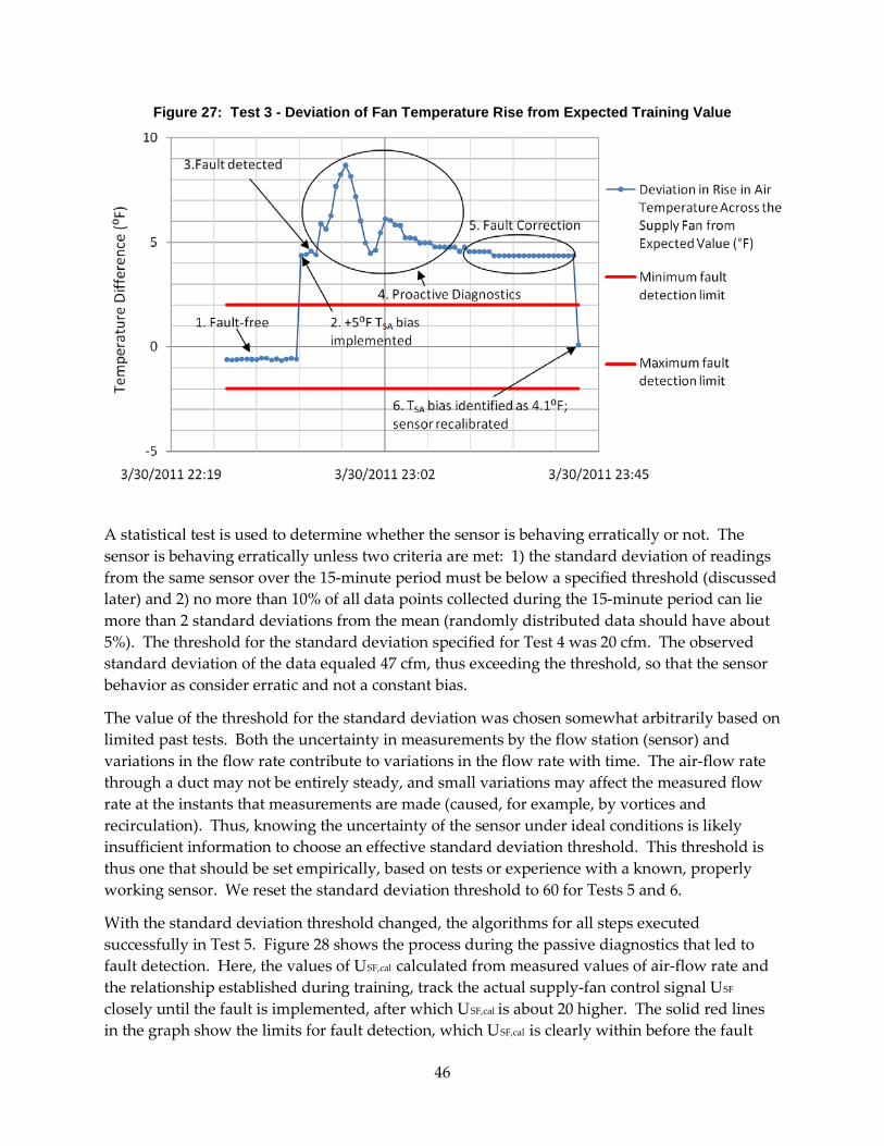
46

Figure 27: Test 3 - Deviation of Fan Temperature Rise from Expected Training Value

A statistical test is used to determine whether the sensor is behaving erratically or not. The sensor is behaving erratically unless two criteria are met: 1) the standard deviation of readings from the same sensor over the 15-minute period must be below a specified threshold (discussed later) and 2) no more than 10% of all data points collected during the 15-minute period can lie more than 2 standard deviations from the mean (randomly distributed data should have about 5%). The threshold for the standard deviation specified for Test 4 was 20 cfm. The observed standard deviation of the data equaled 47 cfm, thus exceeding the threshold, so that the sensor behavior as consider erratic and not a constant bias.

The value of the threshold for the standard deviation was chosen somewhat arbitrarily based on limited past tests. Both the uncertainty in measurements by the flow station (sensor) and variations in the flow rate contribute to variations in the flow rate with time. The air-flow rate through a duct may not be entirely steady, and small variations may affect the measured flow rate at the instants that measurements are made (caused, for example, by vortices and recirculation). Thus, knowing the uncertainty of the sensor under ideal conditions is likely insufficient information to choose an effective standard deviation threshold. This threshold is thus one that should be set empirically, based on tests or experience with a known, properly working sensor. We reset the standard deviation threshold to 60 for Tests 5 and 6.

With the standard deviation threshold changed, the algorithms for all steps executed successfully in Test 5. Figure 28 shows the process during the passive diagnostics that led to fault detection. Here, the values of USF,cal calculated from measured values of air-flow rate and the relationship established during training, track the actual supply-fan control signal USF closely until the fault is implemented, after which USF,cal is about 20 higher. The solid red lines in the graph show the limits for fault detection, which USF,cal is clearly within before the fault

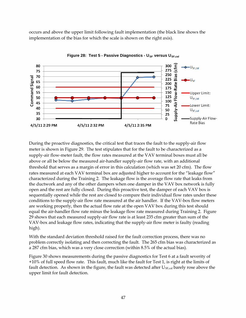
47

occurs and above the upper limit following fault implementation (the black line shows the implementation of the bias for which the scale is shown on the right axis).

Figure 28: Test 5 - Passive Diagnostics - USF versus USF,cal

During the proactive diagnostics, the critical test that traces the fault to the supply-air flow meter is shown in Figure 29. The test stipulates that for the fault to be characterized as a supply-air flow-meter fault, the flow rates measured at the VAV terminal boxes must all be above or all be below the measured air-handler supply-air flow rate, with an additional threshold that serves as a margin of error in this calculation (which was set 20 cfm). The flow rates measured at each VAV terminal box are adjusted higher to account for the “leakage flow” characterized during the Training 2. The leakage flow is the average flow rate that leaks from the ductwork and any of the other dampers when one damper in the VAV box network is fully open and the rest are fully closed. During this proactive test, the damper of each VAV box is sequentially opened while the rest are closed to compare their individual flow rates under these conditions to the supply-air flow rate measured at the air handler. If the VAV-box flow meters are working properly, then the actual flow rate at the open VAV box during this test should equal the air-handler flow rate minus the leakage flow rate measured during Training 2. Figure 29 shows that each measured supply-air flow rate is at least 235 cfm greater than sum of the VAV-box and leakage flow rates, indicating that the supply-air flow meter is faulty (reading high).

With the standard deviation threshold raised for the fault correction process, there was no problem correctly isolating and then correcting the fault. The 265 cfm bias was characterized as a 287 cfm bias, which was a very close correction (within 8.5% of the actual bias).

Figure 30 shows measurements during the passive diagnostics for Test 6 at a fault severity of +10% of full speed flow rate. This fault, much like the fault for Test 1, is right at the limits of fault detection. As shown in the figure, the fault was detected after USF,cal barely rose above the upper limit for fault detection.

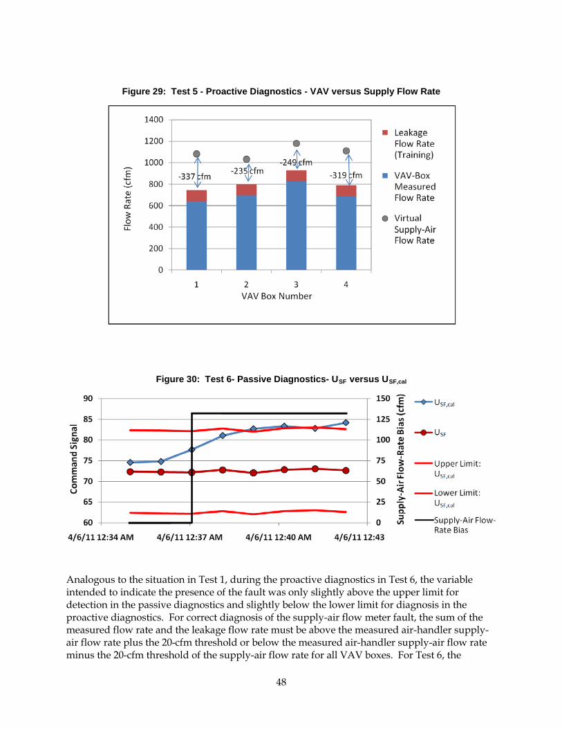
48

Figure 29: Test 5 - Proactive Diagnostics - VAV versus Supply Flow Rate

Figure 30: Test 6- Passive Diagnostics- USF versus USF,cal

Analogous to the situation in Test 1, during the proactive diagnostics in Test 6, the variable intended to indicate the presence of the fault was only slightly above the upper limit for detection in the passive diagnostics and slightly below the lower limit for diagnosis in the proactive diagnostics. For correct diagnosis of the supply-air flow meter fault, the sum of the measured flow rate and the leakage flow rate must be above the measured air-handler supply-air flow rate plus the 20-cfm threshold or below the measured air-handler supply-air flow rate minus the 20-cfm threshold of the supply-air flow rate for all VAV boxes. For Test 6, the

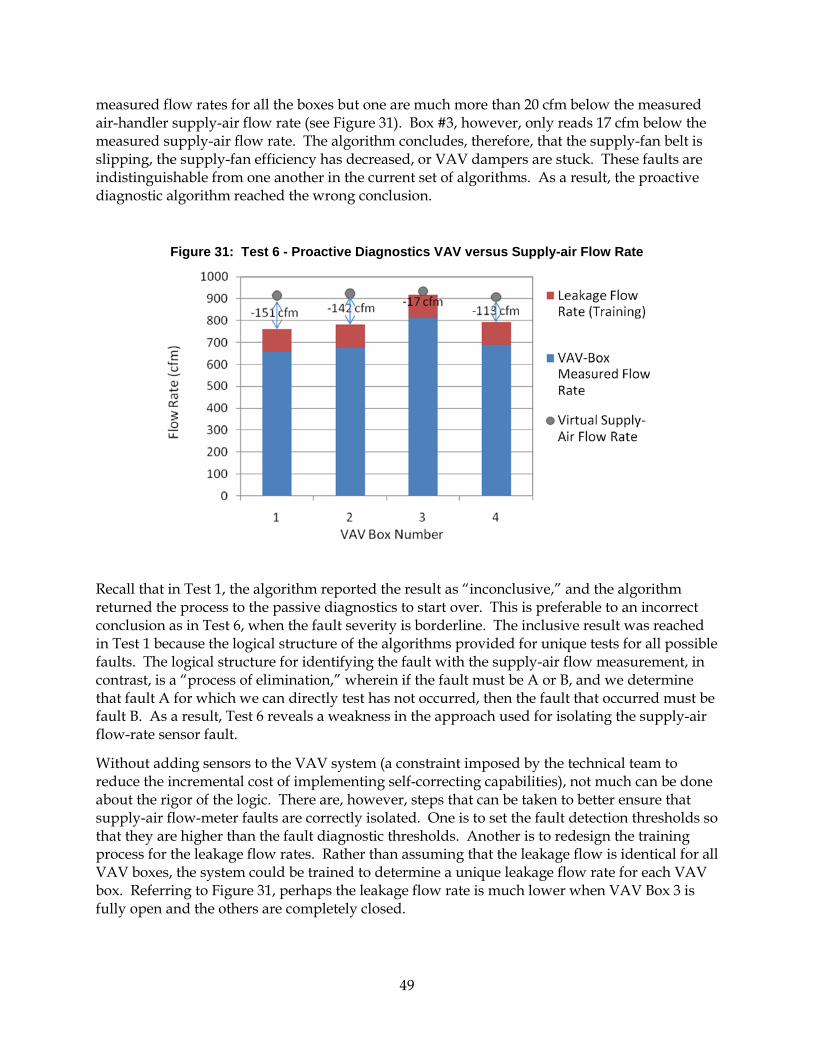
49

measured flow rates for all the boxes but one are much more than 20 cfm below the measured air-handler supply-air flow rate (see Figure 31). Box #3, however, only reads 17 cfm below the measured supply-air flow rate. The algorithm concludes, therefore, that the supply-fan belt is slipping, the supply-fan efficiency has decreased, or VAV dampers are stuck. These faults are indistinguishable from one another in the current set of algorithms. As a result, the proactive diagnostic algorithm reached the wrong conclusion.

Figure 31: Test 6 - Proactive Diagnostics VAV versus Supply-air Flow Rate

Recall that in Test 1, the algorithm reported the result as “inconclusive,” and the algorithm returned the process to the passive diagnostics to start over. This is preferable to an incorrect conclusion as in Test 6, when the fault severity is borderline. The inclusive result was reached in Test 1 because the logical structure of the algorithms provided for unique tests for all possible faults. The logical structure for identifying the fault with the supply-air flow measurement, in contrast, is a “process of elimination,” wherein if the fault must be A or B, and we determine that fault A for which we can directly test has not occurred, then the fault that occurred must be fault B. As a result, Test 6 reveals a weakness in the approach used for isolating the supply-air flow-rate sensor fault.

Without adding sensors to the VAV system (a constraint imposed by the technical team to reduce the incremental cost of implementing self-correcting capabilities), not much can be done about the rigor of the logic. There are, however, steps that can be taken to better ensure that supply-air flow-meter faults are correctly isolated. One is to set the fault detection thresholds so that they are higher than the fault diagnostic thresholds. Another is to redesign the training process for the leakage flow rates. Rather than assuming that the leakage flow is identical for all VAV boxes, the system could be trained to determine a unique leakage flow rate for each VAV box. Referring to Figure 31, perhaps the leakage flow rate is much lower when VAV Box 3 is fully open and the others are completely closed.

50

CHAPTER 4: Economic and Impact Assessment Many faults affecting the energy efficiency and performance of HVAC systems go undetected and uncorrected, often for long periods of time. Even when faults are detected and properly diagnosed, it is common for faults to persist because building operations staff do not find the time to address many of these faults, or HVAC service technicians do not receive approval from building owners to complete the required service or repair. Self-correcting controls could automatically correct many of these faults by reconfiguring controls and recalibrating devices, and thus enable the system to maintain performance efficiency. To estimate the potential energy and economic impacts of deploying self-correcting controls, we first estimate HVAC system-level savings (on average) and then multiply the savings by the potential number of systems impacted. Cost savings and environmental benefits are then derived from the estimated energy savings. To appropriately capture the persistent savings from controls that continually self-correct operational faults, the savings are estimated over a 15-year period based on forecasted building stock and energy price estimates developed by the California Energy Commission (CEC).

Technical and Market Potential Based on published reports, savings between 10% and 30% are generally achievable by correcting operation problems. It is reasonable to assume that systems retrofit with robust self-correcting controls could achieve average HVAC energy savings of 15% over common operation conditions for applicable systems over the lifetime of the system (Mills 2009, Moore et al. 2008, Roth et al. 2005, Tso et al. 2007).

The targeted market will include built-up, central HVAC systems with a longer-term market potential targeting packaged HVAC systems. To determine the energy savings potential for these targeted systems, the energy consumed by various HVAC systems was calculated based on equipment shares derived from California Commercial End-Use Survey (CEUS) data (Itron 2006).3 The CEUS survey queries provided information on equipment shares by building stock and climate zone as well energy consumption by end use. California commercial building stock forecasts were taken from the California Energy Commission’s (CEC’s) most recent energy forecast (CEC 2009). Equipment shares by building type and building stock forecasts were then input into the PNNL-developed Building Energy Analysis Modeling System (BEAMS)4 to derive consumption by equipment type (Elliott et al. 2004).

Overall, the total energy used by both built-up and packaged systems to heat, cool , and ventilate commercial buildings in California is estimated to make up about one-quarter of the total delivered energy use in the overall commercial sector and just over three-quarters of the total delivered commercial HVAC energy use. Figure 33 provides a diagram identifying the

3 CEUS data query received in Excel format from Mark Ciminelli, Senior Mechanical Engineer, California State Demand Analysis Office (10/13/2010). 4 Chapter 2 of referenced report (Elliott et al. 2004) provides a detailed description of “BESET” model, which has since been renamed as “BEAMS.”

51

energy use targeted by self-correcting HVAC controls. The energy use includes both natural gas and electric delivered energy consumption in trillions of British thermal units (TBtus). The initial target, which focuses on built-up systems, only accounts for about 17 % of total HVAC energy use in commercial buildings; however, these self-correcting systems will be available for retrofit, enabling near-term deployment into the existing building stock. Packaged systems make up a much larger portion of the total HVAC delivered energy use (60%); however, the current set of self-correcting controls has not yet been tested or demonstrated on packaged systems, so deployment into this market would likely be further in the future.

Figure 32: Target Market for Self-Correcting Controls (Delivered TBtus)

Methodology The benefit estimates for self-correcting controls are estimated with PNNL’s Building Energy Analysis Modeling System (BEAMS). BEAMS is a bottom-up accounting model that compares baseline energy use against specific energy-efficient technologies or energy saving programs (Elliott et al. 2004). The BEAMS model baseline was calibrated to represent the California commercial building energy market. The underlying building stock assumptions and forecast are based on the most recent CEC energy forecast (CEC 2009), while HVAC equipment market shares by building type are based on CEUS survey results (Itron 2006). Average equipment efficiencies were drawn primarily from the Department of Energy’s (DOE’s) National Energy Modeling System (NEMS) input assumptions (EIA 2010). The baseline also includes heating and cooling end-use loads representing the baseline heating and cooling energy use per square foot. To appropriately represent the savings in a particular sector, the baseline includes commercial building end-use loads developed for specific building types (e.g., education, large office, etc.) as well as by vintage for two encompassing California climate zones. End-use loads were derived from the Facility Energy Decision System (FEDS) to reflect current energy technology and consumption behavior (PNNL 2008).

The market penetration over time is developed based on market diffusion curves developed by PNNL, which are based on a Bass diffusion model (Bass 1969) for various building HVAC

Total Statewide Commercial Building Energy Consumption (2009)

538.6 TBtu

HVAC Use 171.1 TBtu

Built-up Systems and Packaged Systems Annual Energy Use 131.6 TBtu

Built-up: 29.2 TBtu

Packaged Systems: 102.4 TBtu

Near-term target

Longer Term Target

Self-Correcting Controls Applicable to Built-Up HVAC Systems and potentially applicable for Packaged HVAC Systems

Self-Correcting Controls targeting HVAC (Exclude Lighting, Water Heat, Plug Loads, and other Commercial Building Energy from technical potential)

52

technologies (Elliott et al. 20045). Bass was the first to suggest the “S” curve or logistic functional form for the market diffusion of new products, and his concepts are still widely employed in the marketing discipline today. The model development and empirical analysis were designed to generate more credible predictions of the adoption process of energy-efficiency technologies in the buildings sector. The timeframe for this study is limited to a 15-year period.

Built-up System Savings The initial set of self-correction methods and algorithms developed as part of this project are being tested and demonstrated on built-up HVAC systems. Built-up HVAC systems are characterized as central HVAC systems that are custom-designed for a building. Chillers and boilers make up the source components for the vast majority of the built-up systems in the California commercial building stock; however, a small percentage of the built-up systems are supplied with other HVAC source components (e.g., central air-conditioning and gas furnaces). The shares of built-up systems are identified with CEUS data queries to characterize the market potential and market penetration of self-correcting controls into this market.

Two deployment paths were considered related to the deployment of self-correcting controls into the built-up HVAC market:

Deployment Path 1: Deployment of self-correcting controls as software code in an energy management and control system or building automations systems (BAS) in commercial buildings or as a third-party software connected to a BAS; and Deployment Path 2: Deployment by integrating self-correcting code into distributed field panels or device controllers.

Although BAS are found in relatively few buildings overall (5% of buildings encompassing approximately 17% of commercial floor space), they are much more prevalent in buildings that have built-up systems. Based on data queries from the Energy Information Administration (EIA) Commercial Buildings Energy Consumption Survey (CBECS), it is estimated that approximately 50% to 70% of commercial floor space served with built-up systems in California is equipped with building automation systems (EIA 2003). Deployment through a BAS system would, therefore, provide significant opportunities to penetrate buildings with a newly installed BAS; but more importantly, it would also provide opportunities to retrofit and impact a large fraction of the existing building stock because these systems could be retrofit more easily and cost effectively with self-correcting controls. The second deployment path, “Deployment by integrating self-correcting code into distributed field panels or device controllers “ would also provide opportunities to reduce energy use within the existing building stock; however, the opportunity for retrofit would more likely come as system components are retired and changed out or upgraded, which would be a much slower process.

To assess the energy market and economic impact of self-correcting controls in the built-up market, it was assumed that a very aggressive market deployment program could achieve 40%

5 See Chapter 3, “Technology Diffusion Models – Application to Selected Energy-Efficient Products for Buildings,” of Elliott et al. for more information on development of diffusion models. Sources for HVAC technology data and conclusions include Census of Manufacturers, Gas Appliance Manufacturers Association (GAMA) [Srinivasan & Mason (1986); Brown et al. (1989); Mahajan, Mason, and Srinivasan (1986)].

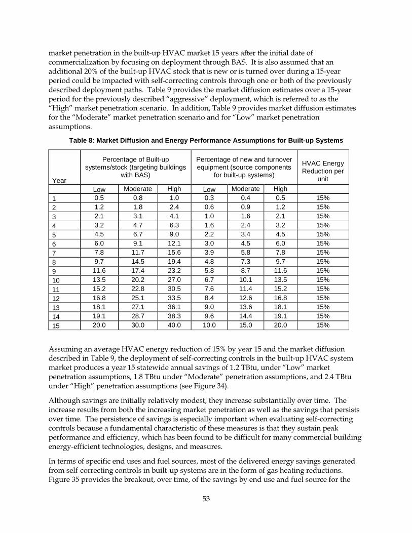
53

market penetration in the built-up HVAC market 15 years after the initial date of commercialization by focusing on deployment through BAS. It is also assumed that an additional 20% of the built-up HVAC stock that is new or is turned over during a 15-year period could be impacted with self-correcting controls through one or both of the previously described deployment paths. Table 9 provides the market diffusion estimates over a 15-year period for the previously described “aggressive” deployment, which is referred to as the “High” market penetration scenario. In addition, Table 9 provides market diffusion estimates for the “Moderate” market penetration scenario and for “Low” market penetration assumptions.

Table 8: Market Diffusion and Energy Performance Assumptions for Built-up Systems

Year

Percentage of Built-up systems/stock (targeting buildings

with BAS)

Percentage of new and turnover equipment (source components

for built-up systems)

HVAC Energy Reduction per

unit Low Moderate High Low Moderate High

1 0.5 0.8 1.0 0.3 0.4 0.5 15% 2 1.2 1.8 2.4 0.6 0.9 1.2 15% 3 2.1 3.1 4.1 1.0 1.6 2.1 15% 4 3.2 4.7 6.3 1.6 2.4 3.2 15% 5 4.5 6.7 9.0 2.2 3.4 4.5 15% 6 6.0 9.1 12.1 3.0 4.5 6.0 15% 7 7.8 11.7 15.6 3.9 5.8 7.8 15% 8 9.7 14.5 19.4 4.8 7.3 9.7 15% 9 11.6 17.4 23.2 5.8 8.7 11.6 15% 10 13.5 20.2 27.0 6.7 10.1 13.5 15% 11 15.2 22.8 30.5 7.6 11.4 15.2 15% 12 16.8 25.1 33.5 8.4 12.6 16.8 15% 13 18.1 27.1 36.1 9.0 13.6 18.1 15% 14 19.1 28.7 38.3 9.6 14.4 19.1 15% 15 20.0 30.0 40.0 10.0 15.0 20.0 15%

Assuming an average HVAC energy reduction of 15% by year 15 and the market diffusion described in Table 9, the deployment of self-correcting controls in the built-up HVAC system market produces a year 15 statewide annual savings of 1.2 TBtu, under “Low” market penetration assumptions, 1.8 TBtu under “Moderate” penetration assumptions, and 2.4 TBtu under “High” penetration assumptions (see Figure 34).

Although savings are initially relatively modest, they increase substantially over time. The increase results from both the increasing market penetration as well as the savings that persists over time. The persistence of savings is especially important when evaluating self-correcting controls because a fundamental characteristic of these measures is that they sustain peak performance and efficiency, which has been found to be difficult for many commercial building energy-efficient technologies, designs, and measures.

In terms of specific end uses and fuel sources, most of the delivered energy savings generated from self-correcting controls in built-up systems are in the form of gas heating reductions. Figure 35 provides the breakout, over time, of the savings by end use and fuel source for the

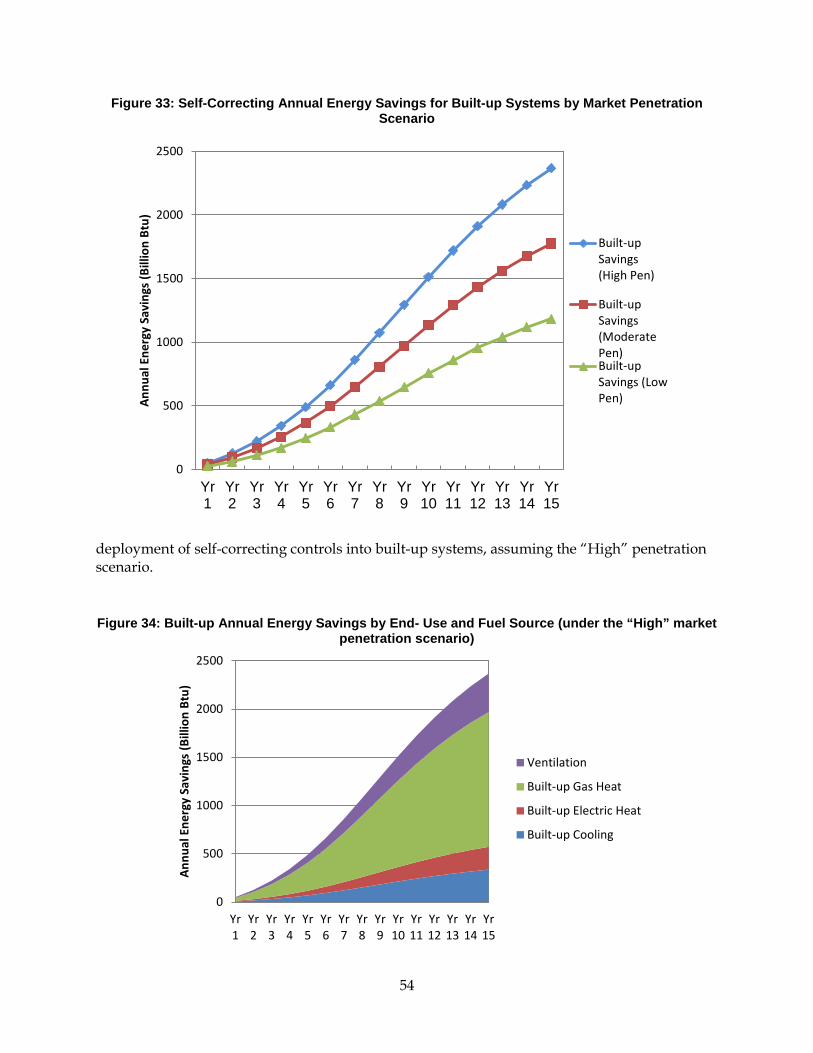
54

Figure 33: Self-Correcting Annual Energy Savings for Built-up Systems by Market Penetration Scenario

deployment of self-correcting controls into built-up systems, assuming the “High” penetration scenario.

Figure 34: Built-up Annual Energy Savings by End- Use and Fuel Source (under the “High” market penetration scenario)

0

500

1000

1500

2000

2500

Yr1

Yr2

Yr3

Yr4

Yr5

Yr6

Yr7

Yr8

Yr9

Yr10

Yr11

Yr12

Yr13

Yr14

Yr15

Annu

al E

nerg

y Sa

ving

s (B

illio

n Bt

u)

Built-upSavings(High Pen)

Built-upSavings(ModeratePen)Built-upSavings (LowPen)

0

500

1000

1500

2000

2500

Yr1

Yr2

Yr3

Yr4

Yr5

Yr6

Yr7

Yr8

Yr9

Yr10

Yr11

Yr12

Yr13

Yr14

Yr15

Annu

al E

nerg

y Sa

ving

s (B

illio

n Bt

u)

Ventilation

Built-up Gas Heat

Built-up Electric Heat

Built-up Cooling

55

Built-up system savings from self-correcting controls are concentrated in a few building types, with the miscellaneous building category (e.g., public assembly, religious, etc.), education, and large offices6 making up just over 85% of the savings (see Figure 36) 10 years after the initial deployment. Health care facilities make up an addition 11% of the savings.

Figure 35: Percent of Savings in Built-up Systems by Building Type

Packaged System Savings Although the self-correcting controls developed as part of this project have not been directly tested or demonstrated on packaged systems, it is believed that the algorithms developed for built-up systems could be tailored to packaged systems to achieve similar performance benefits. Packaged systems are the most common HVAC systems in commercial buildings and make up 60% of the total HVAC energy consumption in California. Thus, any measure that improves the performance of packaged systems, in general, could have significant energy reduction impacts. Because packaged systems tend to be serviced less than built-up systems and are less likely to be affiliated with a BAS, there would likely be fewer opportunities to retrofit existing packaged systems with self-correcting controls. The pathway for deployment of self-correcting controls would therefore more likely occur at the equipment production level for packaged systems. There are five well known manufacturers of commercial HVAC equipment that dominate the market: Carrier, Lennox, McQuay, Trane, and York. Based on a 2005 Northwest Energy Efficiency Alliance (NEEA) study, the “Big Three” manufacturers for packaged heating and cooling equipment used in the Pacific Northwest are Trane, Carrier, and Lennox, where Trane is estimated to have 50% of the market share, followed by Carrier (30%), and Lennox (15%) (NEEA 2005). Other manufacturers, mainly York, are estimated to have 5% of the packaged HVAC commercial market share. Assuming that the California HVAC market is similar to the Northwest and low-cost self-correcting controls were available and could be integrated into a packaged system during fabrication, only one or two companies would need to integrate these capabilities into their systems to provide a sizable impact on HVAC energy consumption. 6 “Large offices” are defined as office buildings equal to or greater than 30,000 square feet.

Misc/Assembly

53% Education

18%

Office-Large 15%

Health Care 11%

Lodging 2%

All Other 1%

56

To assess the energy and economic impacts of self-correcting controls in the packaged system market, it was assumed that an aggressive market deployment program could achieve 40% of the packaged system HVAC stock that are new or replacement units during a 15-year period.7 This would not include the fraction of existing packaged systems that could potentially be retrofit to incorporate self-correcting controls. Table 10 provides the market diffusion estimates for a “Low,” “Moderate,” and “High” market penetration scenarios over a 15-year period.

As shown in Figure 37, even while only penetrating into new equipment, the energy savings potential for deploying self-correcting controls into packaged systems is significant because of the prevalence of these systems. By year 15, annual savings reach 3.8 TBtus under the scenario with “High” market penetration assumptions, 2.8 TBtus under the “Moderate” market penetration scenario and 1.9 TBTus under the “Low” market penetration assumptions.

The savings generated from self-correcting controls deployed in packaged systems comes primarily in the form of natural gas heat savings and cooling savings. Figure 38 provides the breakout, over time, of the savings by end use and fuel source for the deployment of self-correcting controls into packaged systems, assuming the “High” penetration scenario.

Table 9: Market Diffusion and Energy Performance Assumptions for Packaged Systems

Year Percentage of new and turnover package system equipment

HVAC Energy Reduction per

unit Low Moderate High 1 0.5 0.8 1.0 15% 2 1.2 1.8 2.4 15% 3 2.1 3.1 4.1 15% 4 3.2 4.7 6.3 15% 5 4.5 6.7 9.0 15% 6 6.0 9.1 12.1 15% 7 7.8 11.7 15.6 15% 8 9.7 14.5 19.4 15% 9 11.6 17.4 23.2 15%

10 13.5 20.2 27.0 15% 11 15.2 22.8 30.5 15% 12 16.8 25.1 33.5 15% 13 18.1 27.1 36.1 15% 14 19.1 28.7 38.3 15% 15 20.0 30.0 40.0 15%

7 Although packaged system impacts would not be expected in the near-term, the impacts for a 15-year period are projected during the same 15-year period as the built-up systems for convenience and to coordinate with the CEC building and price forecasts.

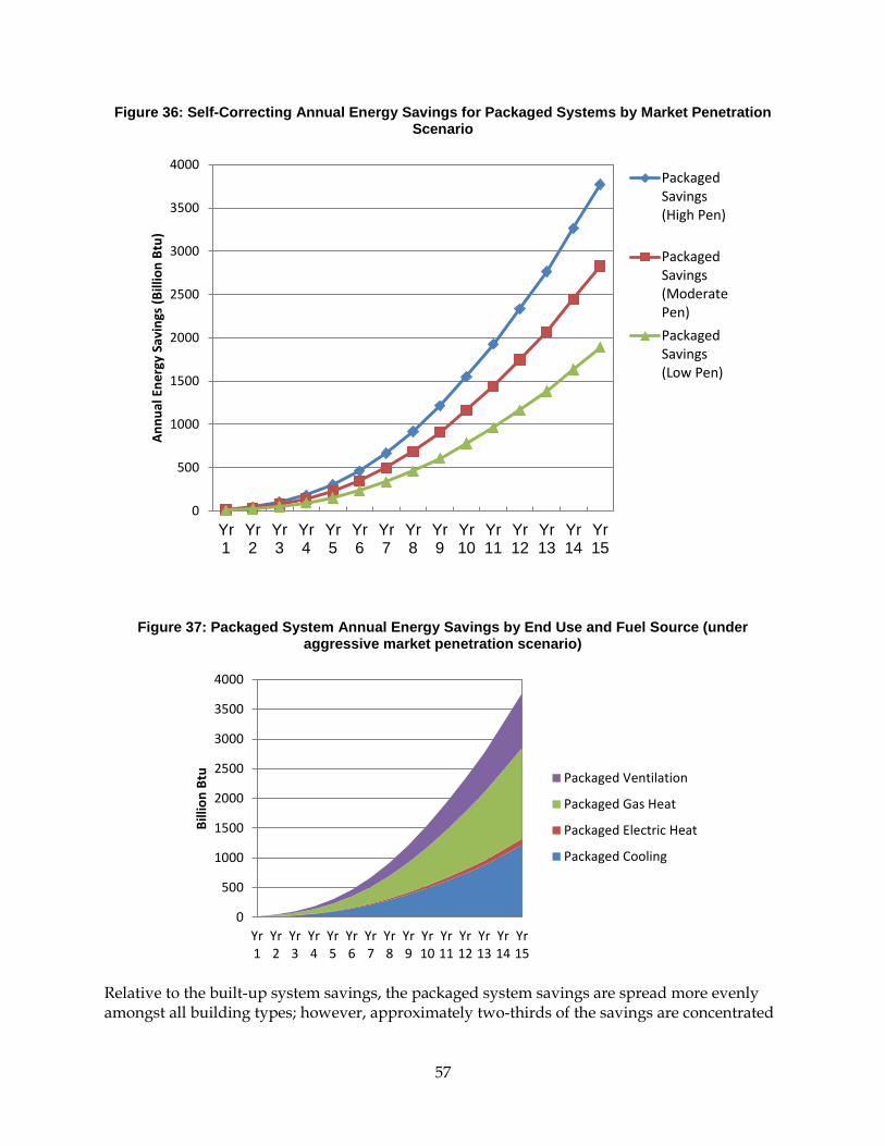
57

Figure 36: Self-Correcting Annual Energy Savings for Packaged Systems by Market Penetration Scenario

Figure 37: Packaged System Annual Energy Savings by End Use and Fuel Source (under aggressive market penetration scenario)

Relative to the built-up system savings, the packaged system savings are spread more evenly amongst all building types; however, approximately two-thirds of the savings are concentrated

0

500

1000

1500

2000

2500

3000

3500

4000

Yr1

Yr2

Yr3

Yr4

Yr5

Yr6

Yr7

Yr8

Yr9

Yr10

Yr11

Yr12

Yr13

Yr14

Yr15

Annu

al E

nerg

y Sa

ving

s (B

illio

n Bt

u)

PackagedSavings(High Pen)

PackagedSavings(ModeratePen)PackagedSavings(Low Pen)

0

500

1000

1500

2000

2500

3000

3500

4000

Yr1

Yr2

Yr3

Yr4

Yr5

Yr6

Yr7

Yr8

Yr9

Yr10

Yr11

Yr12

Yr13

Yr14

Yr15

Billi

on B

tu

Packaged Ventilation

Packaged Gas Heat

Packaged Electric Heat

Packaged Cooling

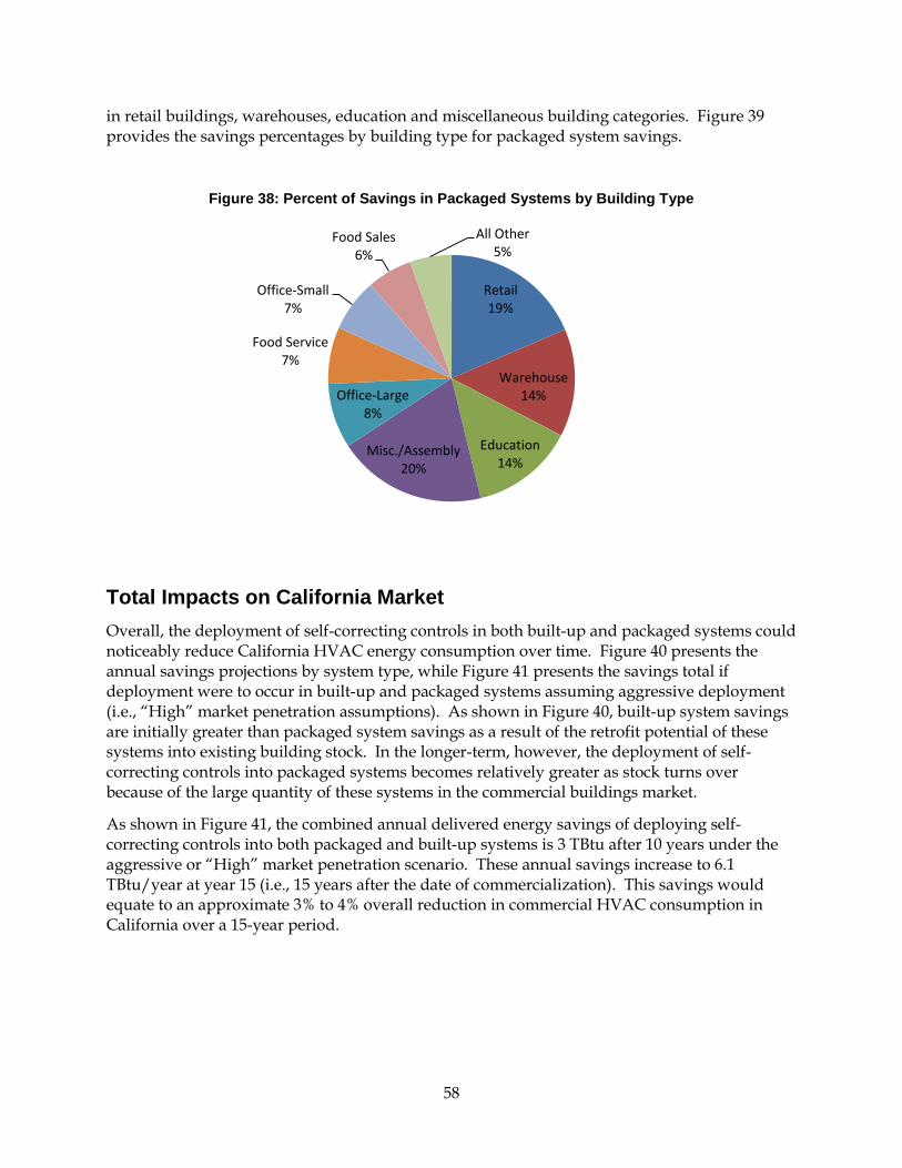
58

in retail buildings, warehouses, education and miscellaneous building categories. Figure 39 provides the savings percentages by building type for packaged system savings.

Figure 38: Percent of Savings in Packaged Systems by Building Type

Total Impacts on California Market Overall, the deployment of self-correcting controls in both built-up and packaged systems could noticeably reduce California HVAC energy consumption over time. Figure 40 presents the annual savings projections by system type, while Figure 41 presents the savings total if deployment were to occur in built-up and packaged systems assuming aggressive deployment (i.e., “High” market penetration assumptions). As shown in Figure 40, built-up system savings are initially greater than packaged system savings as a result of the retrofit potential of these systems into existing building stock. In the longer-term, however, the deployment of self-correcting controls into packaged systems becomes relatively greater as stock turns over because of the large quantity of these systems in the commercial buildings market.

As shown in Figure 41, the combined annual delivered energy savings of deploying self-correcting controls into both packaged and built-up systems is 3 TBtu after 10 years under the aggressive or “High” market penetration scenario. These annual savings increase to 6.1 TBtu/year at year 15 (i.e., 15 years after the date of commercialization). This savings would equate to an approximate 3% to 4% overall reduction in commercial HVAC consumption in California over a 15-year period.

Retail 19%

Warehouse 14%

Education 14%

Misc./Assembly 20%

Office-Large 8%

Food Service 7%

Office-Small 7%

Food Sales 6%

All Other 5%

59

Figure 39: Self-Correcting Annual Energy Savings by System Type with Aggressive Market Deployment Assumptions (i.e., “High Pen”)

Figure 40: Total Delivered Annual Energy Savings (both electric and natural gas) with Deployment into both Built-up and Packaged Systems (High Market Penetration Scenario)

Economic Impact The energy cost savings associated with the energy savings presented in Figure 41 are shown in Figure 42. Cost savings are derived by multiplying the savings (by energy type) by the delivered energy price, which are forecasted by the CEC8. In the near-term (year 5), the self- 8 Prices forecasted by CEC out to the year 2020. Beyond 10 years, prices were held constant at 2020 prices.

0

500

1000

1500

2000

2500

3000

3500

4000

Yr1

Yr2

Yr3

Yr4

Yr5

Yr6

Yr7

Yr8

Yr9

Yr10

Yr11

Yr12

Yr13

Yr14

Yr15

Billi

on B

tu

Built-up SystemSavings

Packaged SystemSavings

0

1000

2000

3000

4000

5000

6000

7000

Yr1

Yr2

Yr3

Yr4

Yr5

Yr6

Yr7

Yr8

Yr9

Yr10

Yr11

Yr12

Yr13

Yr14

Yr15

Ann

ual E

nerg

y Sa

ving

s (B

illio

n Bt

u)

PackagedSystemSavings

Built-upSystemSavings

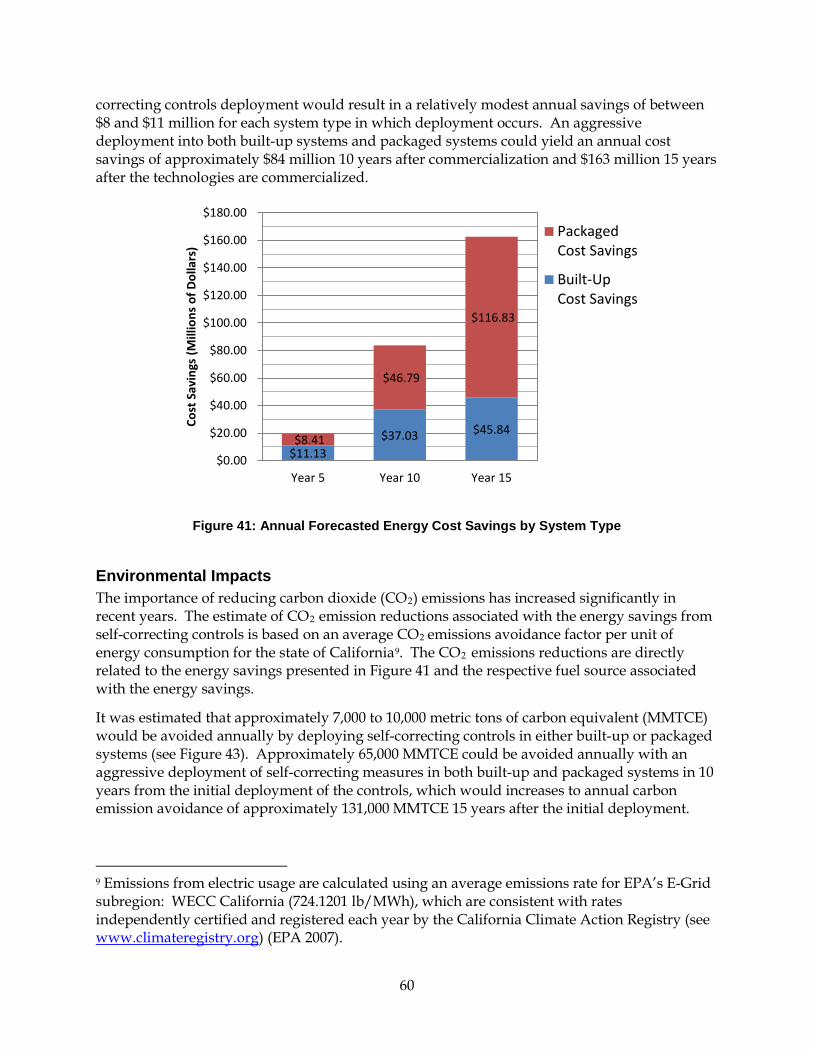
60

correcting controls deployment would result in a relatively modest annual savings of between $8 and $11 million for each system type in which deployment occurs. An aggressive deployment into both built-up systems and packaged systems could yield an annual cost savings of approximately $84 million 10 years after commercialization and $163 million 15 years after the technologies are commercialized.

Figure 41: Annual Forecasted Energy Cost Savings by System Type

Environmental Impacts The importance of reducing carbon dioxide (CO2) emissions has increased significantly in recent years. The estimate of CO2 emission reductions associated with the energy savings from self-correcting controls is based on an average CO2 emissions avoidance factor per unit of energy consumption for the state of California9. The CO2 emissions reductions are directly related to the energy savings presented in Figure 41 and the respective fuel source associated with the energy savings.

It was estimated that approximately 7,000 to 10,000 metric tons of carbon equivalent (MMTCE) would be avoided annually by deploying self-correcting controls in either built-up or packaged systems (see Figure 43). Approximately 65,000 MMTCE could be avoided annually with an aggressive deployment of self-correcting measures in both built-up and packaged systems in 10 years from the initial deployment of the controls, which would increases to annual carbon emission avoidance of approximately 131,000 MMTCE 15 years after the initial deployment.

9 Emissions from electric usage are calculated using an average emissions rate for EPA’s E-Grid subregion: WECC California (724.1201 lb/MWh), which are consistent with rates independently certified and registered each year by the California Climate Action Registry (see www.climateregistry.org) (EPA 2007).

$11.13 $37.03 $45.84

$8.41

$46.79

$116.83

$0.00

$20.00

$40.00

$60.00

$80.00

$100.00

$120.00

$140.00

$160.00

$180.00

Year 5 Year 10 Year 15

Cost

Sav

ings

(Mill

ions

of D

olla

rs)

PackagedCost Savings

Built-UpCost Savings

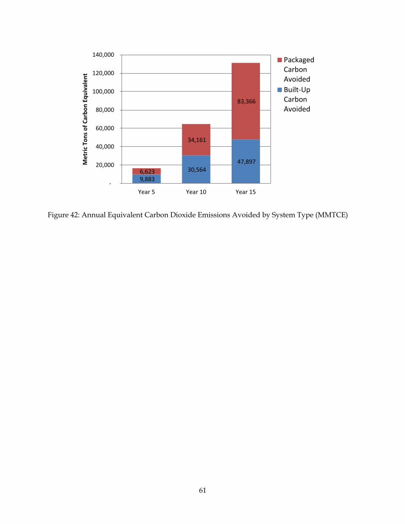
61

Figure 42: Annual Equivalent Carbon Dioxide Emissions Avoided by System Type (MMTCE)

9,883 30,564

47,897 6,623

34,161

83,366

-

20,000

40,000

60,000

80,000

100,000

120,000

140,000

Year 5 Year 10 Year 15

Met

ric T

ons o

f Car

bon

Equi

vale

nt

PackagedCarbonAvoidedBuilt-UpCarbonAvoided

62

CHAPTER 5: Future Work Proposed future work falls into three categories: 1) improved models and procedures for collecting training data, 2) completion of the full suite of tests necessary to validate the fault detection, diagnosis, and correction algorithms for the air handling (filter/fan/coil) and VAV sections, 3) integrating the self-correcting control algorithms with building automation systems other than the Johnson Controls Metasys®10 used for the laboratory tests completed thus far, and 4) field testing the self-correcting control algorithms in operating commercial buildings.

Improved Training Models and Procedures Each of the training algorithms requires modifications.

Training 1 requires only a slight modification. As noted in Chapter 3, no actuator response occurred for command signals under 25% for all dampers and valves in the laboratory system. The model for devices that respond in this manner should be revised to include a region for low values of command signals (e.g., less than 25%) for which no response occurs and a second region (e.g., 25% to 100%) in which the device (e.g., damper or fan) response increases with increasing command signal. A polynomial curve fit can then be used to capture the behavior in this second region. The value of the command signal at which the response becomes non-zero may differ among equipment, controllers and systems, so a step to identify this transition point needs to be added to the Training 1 process and algorithm.

As mentioned in Chapter 3, the leakage flow rate training (in Training 2) should be modified to the determine a leakage flow rate for each of the VAV boxes served by the air handler, rather than averaging the measured leakage flow rates to arrive at one leakage rate used for all VAV boxes.

Training 3 requires a more substantial revision. In hindsight, ΔTSM is inadequate for tracking the performance of the cooling coil. As the difference between the mixed-air temperature and the chilled-water temperature changes, the achievable temperature drop across the cooling coil also changes. The heat exchanger effectiveness, which can be shown as equal to the air-side temperature drop across the cooling coil divided by the thermodynamic maximum temperature drop achievable by the air, would be a better variable for this purpose. For the cooling coil, that temperature drop would be the difference between the air temperature at the cooling-coil inlet and the chilled-water temperature (at the cooling-coil water inlet). The air-temperature leaving the cooling coil is not ordinarily measured; therefore, it must be estimated from the supply-air temperature accounting for the increase in temperature as the cooled air flows past the supply fan (ΔTSF). The change in air temperature across the cooling coil is then estimated as the difference THC – (TSA - ΔTSF) = THC – TSA + ΔTSF, where THC is the air temperature leaving the heating coil but before entering the cooling coil (see Figure 1 for the locations of the sensors). Thus, the cooling-coil effectiveness (εCC) is given in terms of commonly available sensors by

10 Metasys is a registered trademark of Johnson Controls, Inc.

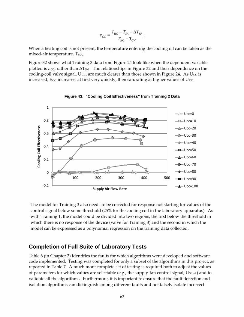
63

.CWHC

SFSAHCCC TT

TTT−

∆+−=ε

When a heating coil is not present, the temperature entering the cooling oil can be taken as the mixed-air temperature, TMA.

Figure 32 shows what Training 3 data from Figure 24 look like when the dependent variable plotted is εCC, rather than ΔTSM. The relationships in Figure 32 and their dependence on the cooling-coil valve signal, UCC, are much clearer than those shown in Figure 24. As UCC is increased, ECC increases. at first very quickly, then saturating at higher values of UCC.

Figure 43: "Cooling Coil Effectiveness" from Training 2 Data

The model for Training 3 also needs to be corrected for response not starting for values of the control signal below some threshold (25% for the cooling coil in the laboratory apparatus). As with Training 1, the model could be divided into two regions, the first below the threshold in which there is no response of the device (valve for Training 3) and the second in which the model can be expressed as a polynomial regression on the training data collected.

Completion of Full Suite of Laboratory Tests Table 6 (in Chapter 3) identifies the faults for which algorithms were developed and software code implemented. Testing was completed for only a subset of the algorithms in this project, as reported in Table 7. A much more complete set of testing is required both to adjust the values of parameters for which values are selectable (e.g., the supply-fan control signal, USF,tol ) and to validate all the algorithms. Furthermore, it is important to ensure that the fault detection and isolation algorithms can distinguish among different faults and not falsely isolate incorrect

-0.2

0

0.2

0.4

0.6

0.8

1

0 100 200 300 400 500

Cool

ing

Coil

Effe

ctiv

enes

s

Supply Air Flow Rate

Ucc=0

Ucc=10

Ucc=20

Ucc=30

Ucc=40

Ucc=50

Ucc=60

Ucc=70

Ucc=80

Ucc=90

Ucc=100

64

faults. This will require testing the algorithms with many different faults, even those which are not correctable, as part of ensuring that false positive fault detection and incorrect fault isolation are minimized. Table 8 provides a list of all detectable VAV system faults identified in this project. Many of these faults would be trivial to detect, but the algorithms for their detection have not been coded in software yet to enable testing. Most of these faults are not self- correctable. Nevertheless, demonstrating that all faults can be successfully distinguished from one another is important. A key goal of the self-correcting controls process is not to “fix” faults that don’t exist, which requires minimization of false positive fault detection and errors in fault isolation. Beyond proving this ability, performing tests on all of the faults will reveal weaknesses in the algorithms, which can then be used to formulate important improvements.

Table 10: Testing Status for all Faults in Filter/Fan/Coil and VAV-Box Sections of VAV Systems

Type of Fault Fault Tested? Comments

Hunting CC valve No

HC/CC valve controller software logic fault No

Fan controller software logic fault No

Supply-air flow station complete failure No

Supply-air fan complete failure No

Supply-air fan belt slipping/decreased fan η No

Supply-air flow station biased Yes

Supply-air flow station erratic No

CC valve stuck open or leaking No

HC valve stuck open or leaking N/A No heating coil in lab apparatus

MA temperature sensor biased Yes Tested in mixing-box tests (see Fernandez et al. 2009b)

MA temperature sensor erratic/not working No

HC temperature sensor biased N/A No heating coil in lab apparatus

HC temperature sensor erratic/not working N/A

SA temperature sensor biased Yes Algorithms working well

SA temperature sensor erratic/not working No

Filter is clogged/oversized No

Filter differential pressure sensor biased/ erratic/not working

No

65

Type of Fault Fault Tested? Comments

Filter has fallen down or is installed incorrectly No

VAV box damper does not modulate in upper half of signal range

No

VAV box damper does not modulate in lower half of signal range

No

VAV box flow sensor is biased No

VAV box reheat coil valve stuck open or leaking

No

Discharge air temperature sensor biased No

Discharge air temperature sensor erratic/not working

No

VAV box flow station erratic/ not working No

VAV box damper stuck No

VAV box incorrect maximum flow set point No

Integrating with Additional BASs and Field Testing Although the self-correcting control algorithms should be compatible with any building automation system, the linkages may vary from one BAS to another. Therefore, to ensure compatibility with the variety of BASs found in commercial buildings, the algorithms should be connected to and laboratory tested with BASs other than the Johnson Controls Metasys system used in the laboratory apparatus. The PNNL laboratory has the capability for such testing and will provide a suitable environment for such testing.

Field testing frequently identifies needs and issues not anticipated during initial development and laboratory testing. In preparation for commercial application, tests of the self-correcting control algorithms should be performed in operating commercial buildings to ensure compatibility with actual conditions in the field.

Path Forward Given the status of the algorithms and testing, additional algorithm development and testing is clearly needed; however, even in the current state, a practical self-correcting control capability could be moved to field testing and commercial use relatively soon. The current plans of the PNNL project team, in addition to furthering development and testing, are to develop a field deployable, user compatible, software module for fault detection, isolation and correction for mixing-box sensors of air handlers. These algorithms have proven to perform well in

66

laboratory tests and, therefore, with limited additional laboratory testing, could be moved to field use. The team anticipates applying software for this purpose first to built-up air handlers (rather than air handling in packaged rooftop HVAC units).

As field test results provide data on the field performance of the algorithms and software as well as the prevalence and incidence of faults in the field, that information will be used to update the assessment of economic, energy and power demand impacts.

67

REFERENCES

Bass, F.M. 1969. “A New Product Growth Model for Consumer Durables.” Management Science, Vol. 15 (5): pp. 215-227, January 1969.

Brown, M.A., L.G. Berry, and R.K. Goel. 1989. Commercializing Government-Sponsored Innovations:

Brown, M.A., L.G. Bery, R.A. Balzer, E. Faby. 1993. National Impacts of the Weatherization Assistance Program in Single-Family and Small Multifamily Dwellings. ORNL/CON-326. Oak Ridge National Laboratory, Oak Ridge, Tennessee.

California Energy Commission (CEC) 2009. California Energy Demand 2010-2020 Adopted Forecast. CEC-200-2009-012-CMF, California Energy Commission, Sacramento, California.

Dexter, A. and J. Pakanen, eds. 2001. Demonstrating automated fault detection and diagnosis methods in real buildings. International Energy Agency Annex 34, Technical Research Centre of Finland, Espoo, Finland.

Elliott DB, DM Anderson, DB Belzer, KA Cort, JA Dirks, and DJ Hostick. 2004. Methodological Framework for Analysis of Building-Related Programs: The GPRA Metrics Effort, June 2004. PNNL-14696, Pacific Northwest National Laboratory, Richland, WA. Available at: http://www.pnl.gov/main/publications/external/technical_reports/PNNL-14696.pdf.

Energy Information Administration (EIA). 2003. Commercial Building Energy Use Survey (CBECS) 2003. U.S. Department of Energy. Washington, D.C.

Energy Information Administration (EIA). 2010. Annual Energy Outlook 2009. U.S. Department of Energy, Washington, D.C.

Fernandez, N., S. Li, W. Wang and M.R. Brambley (Pacific Northwest National Laboratory). 2011. Self-Correcting Controls for Variable Air Volume (VAV) Systems: Filter/Coil/Fan and VAV Box Sections, California Energy Commission. Publication number: CEC-XXX-2011-XXX.

Fernandez, N., M.R. Brambley and S. Katipamula. 2009a. Self-Correcting HVAC Controls: Algorithms for Sensors and Dampers in Air-Handling Units, PNNL-19104. Pacific Northwest National Laboratory, Richland, WA.

Fernandez, N., M.R. Brambley, S. Katipamula, H. Cho, J. Goddard and L. Dinh. 2009b. Self-Correcting HVAC Controls Project Final Report, PNNL-19074. Pacific Northwest National Laboratory, Richland, WA.

Hyvarinen, J. and S. Karki, eds. 1996. Building Optimization and Fault Diagnosis Source Book. International Energy Agency Annex 25, Technical Research Center of Finland, Espoo, Finaland.

Itron, Inc. 2006. California Commercial End-Use Survey. Survey conducted for California Energy Commission. Publication # CEC-400-2006-005, March 2006.

68

Mahajan, V., C. Mason, and V. Srinivasan. 1986. “An Evaluation of Estimation Procedures for New Product Diffusion Models.” In Innovation Diffusion Models of New Product Acceptance, V. Mahajan and Y. Wind, eds., Ballinger, Cambridge, Massachusetts.

Mills, Evan. 2009. A Golden Opportunity for Reducing Energy Costs and Greenhouse Gas Emissions. Lawrence Berkeley National Laboratory, Berkeley, Caifornia. Available online at: http://cx.lbl.gov/2009-assessment.html.

Moore, E., E. Crowe, A. Robbins and B. Walker. Portland Energy Conservation (PECI). 2008. “Making the Leap: Data and Lessons Learned from Scaling Up Retrocommissioning Programs.” In Proceedings of the 2008 ACEEE Summer Study on Energy Efficiency in Buildings, pp. 4-230 – 4-242, American Council for an Energy Efficient Economy, Washington, D.C.

Northwest Energy Efficiency Alliance (NEEA). 2005. Light Commercial HVAC. Prepared by: Energy and Environmental Analysis. Report #E205-143. Northwest Energy Efficiency Alliance, Portland, OR.

Pacific Northwest National Laboratory (PNNL). 2008. Facility Energy Decision System User’s Guide, Release 6.0. PNNL-17848, Pacific Northwest National Laboratory, Richland, Washington.

Roth, K.W., D. Westphalen, M.Y. Feng, P. Llana and L. Quartararo. 2005. Energy Impact of commercial Building controls and Performance Diagnostics: Market characterization, Energy Impact of Building Faults and Energy Savings Potential. Reference No. 02140-2390, TIAX, Lexington, Massachusetts. Prepared for the U.S. Department of Energy, Washington, D.C.

Smith, V.A. and Bushby, S. 2003. Air Handling Unit and Variable Air Volume Box Diagnostics, Technical Report P-500-03-096-A3, California Energy Commission, Sacramento, California.

Srinivasan, V. and C. Mason 1986. “Nonlinear Least Squares Estimation of New Product Diffusion Models,” Marketing Science. 5 (Spring):169-78.

Tso, Bing, Nick Hall, Peter Lai, and Richard Pulliam. 2007. “How Much Does Retrocommissioning Really Save? Results From Three Commissioning Program Evaluations in California.” In Proceedings from the 2007 International Energy Program Evaluation Conference, Chicago, 170-181. International Energy Program Evaluation Conference, Chicago, IL.

Twelve Successful Buildings Case Studies. ORNL/CON-275, Oak Ridge National Laboratory, Oak Ridge, Tennessee.

U.S. Environmental Protection Agency (EPA) 2007. “EPA’s Emissions & Generation Resource Integrated Database (eGRID): Power Profiler eGRID subregion and GHG emissions finder tool.” Washington, D.C. Located online: http://www.epa.gov/cleanenergy/energy-and-you/how-clean.html.