Ec

OTa

b

c

a

ARA

KTMGFSB

1

elKp

apoier

d

0h

International Journal of Applied Earth Observation and Geoinformation 29 (2014) 67–77

Contents lists available at ScienceDirect

International Journal of Applied Earth Observation andGeoinformation

jo ur nal home page: www.elsev ier .com/ locate / jag

mpirical models for estimating the suspended sedimentoncentration in Amazonian white water rivers using Landsat 5/TM

távio C. Montanhera,b,∗, Evlyn M.L.M. Novoa, Cláudio C.F. Barbosaa, Camilo D. Rennóa,hiago S.F. Silvac

Divisão de Sensoriamento Remoto, Instituto Nacional de Pesquisas Espaciais, 12201-970, São José dos Campos, SP, BrazilDepartamento de Tecnologia, Universidade Estadual de Maringá, 87506-370, Umuarama, PR, BrazilDepartamento de Geografia, Instituto de Geociências e Ciências Exatas (IGCE) – Universidade Estadual Paulista (UNESP), Rio Claro, SP, Brazil

r t i c l e i n f o

rticle history:eceived 28 August 2013ccepted 15 January 2014

eywords:op of atmosphere reflectanceultiple regressionseology of the Amazonluvial sedimentspectral bandsand ratios

a b s t r a c t

Suspended sediment yield is a very important environmental indicator within Amazonian fluvial systems,especially for rivers dominated by inorganic particles, referred to as white water rivers. For vast portionsof Amazonian rivers, suspended sediment concentration (SSC) is measured infrequently or not at all.However, remote sensing techniques have been used to estimate water quality parameters worldwide,from which data for suspended matter is the most successfully retrieved. This paper presents empiricalmodels for SSC retrieval in Amazonian white water rivers using reflectance data derived from Landsat5/TM. The models use multiple regression for both the entire dataset (global model, N = 504) and forfive segmented datasets (regional models) defined by general geological features of drainage basins. Themodels use VNIR bands, band ratios, and the SWIR band 5 as input. For the global model, the adjustedR2 is 0.76, while the adjusted R2 values for regional models vary from 0.77 to 0.89, all significant (p-value < 0.0001). The regional models are subject to the leave-one-out cross validation technique, whichpresents robust results. The findings show that both the average error of estimation and the standard

deviation increase as the SSC range increases. Regional models were more accurate when comparedwith the global model, suggesting changes in optical proprieties of water sampled at different samplingstations. Results confirm the potential for the estimation of SSC from Landsat/TM historical series datafor the 1980s and 1990s, for which the in situ database is scarce. Such estimates supplement the SSCtemporal series, providing a more comprehensive SSC temporal series which may show environmentaldynamics yet unknown.

. Introduction

Suspended sediments affect the biological processes of aquaticcosystems (Sioli, 1984; Kerr, 1995; Wetzel, 2001), floodplain evo-ution (Nanson and Croke, 1992; Walling and He, 1998; Pierce anding, 2008), and siltation of reservoirs, among other engineeringroblems (Thornton et al., 1981; Thornton, 1990).

In the fluvial system of the Amazon River, suspended sediments

re important regulators of ecological processes in rivers and flood-lains (McClain and Naiman, 2008; Junk et al., 2011). As indicatorsf geomorphological processes in the drainage basins, particularlyn the Andes (Aalto et al., 2006; McClain and Naiman, 2008; Babyt al., 2009), suspended sediments may be possible indicators of dis-uption of the balance of drainage basins subject to deforestation.

∗ Corresponding author at: Departamento de Tecnologia, Universidade Estaduale Maringa, 87506-370, Umuarama, PR, Brazil

E-mail address: otaviocmontanher@yahoo.com.br (O.C. Montanher).

303-2434/$ – see front matter © 2014 Elsevier B.V. All rights reserved.ttp://dx.doi.org/10.1016/j.jag.2014.01.001

© 2014 Elsevier B.V. All rights reserved.

Traditional systems for monitoring the suspended load in riversare based on water samples collected in situ, from predeterminedsections, and subsequent laboratory analysis. Despite the accuracyof these methods, the cost and time of acquisition of these sam-ples are high, and the necessary logistics are quite complex, whichresults in a sample distribution that is limited in time and space(Ritchie et al., 1987; Ritchie and Shiebe, 2000; Costa et al., 2012).Furthermore, in remote areas such as Amazonian rivers, samplinglocations are often chosen on the basis of ease of access, and notby spatial representativeness of the sample. This method of dataacquisition, however, is not always adequate to answer questionsinvolving the spatial and temporal variability in the suspended sed-iment concentration (SSC) in the rivers.

Therefore, the SSC database of rivers of the Amazon Basin ischaracterized by low spatial and temporal sampling frequency. The

public domain data provided by ANA (Brazilian National WaterAgency; available at: www.ana.gov.br) exemplify this: there are 97sampling stations throughout the Amazon basin, with 2.72 samplesper year on average for each station. Data provided by the HYBAM

68 O.C. Montanher et al. / International Journal of Applied Earth Observation and Geoinformation 29 (2014) 67–77

F nian wr

pqlmV

sWieWr(snM

atarptsmede

2

ctp

ig. 1. Location of the Amazon Basin in the South American context, and the Amazoespective Landsat 5 scenes.

rogram (http://www.ore-hybam.org) have higher sampling fre-uency, but include narrower time coverage and are limited to

arger Amazonian rivers. Beyond these limitations, in situ samplingay contain errors related to local effects, as noted by Espinozaillar et al. (2012).

The literature validates the application of radiometric data fromatellites to estimate SSC (Curran and Novo, 1988; Mertes, 2002;

ang and Lu, 2010) and show many studies based on Landsatmages (Khorram, 1985; Aranuvachapun and Walling, 1988; Mertest al., 1993; Mertes, 1994; Dekker et al., 2002; Islam et al., 2004;ang et al., 2009). Most of the studies in Case 2 waters, however,

efer to reservoirs, estuarine, lacustrine and coastal environmentsWang et al., 2009). The few studies in rivers are restricted to smallections usually covering only one scene, and involving a limitedumber of dates. Notable exceptions are Martinez et al. (2009),angiarotti et al. (2013) and Espinoza Villar et al. (2013).Data from the Landsat program ensures a wider range of spatial

nd temporal scales for evaluating SSC, given the far-reaching his-oric series of well calibrated images (Markham and Helder, 2012),s well as free access (Wulder et al., 2012, www.dgi.inpe.br). Cur-ently there are good prospects for the extension of the Landsatrogram (Irons et al., 2012; Loveland and Dwyer, 2012), confirminghe importance of the new techniques for the application of Land-at/TM data. Taking into account the limitations of the in situonitoring for the Amazon region, this paper presents a series of

mpirical models to estimate SSC in Amazonian white water rivers,eveloped from the integration of in situ data and radiometric dataxtracted from the Landsat 5/TM sensor.

. Study area

The Amazonian rivers are classified into three main types:lear water, black water and white water rivers (Sioli, 1984). Eachype of water has a distinct optical behavior that is related to thehysical characteristics of the drainage area. White water rivers

hite water rivers in detail, with the location of in situ SSC gauging stations and the

are dominated by suspended sediments from intense erosionprocesses that occur in the Andean chain (McClain and Naiman,2008). The clear water rivers originate in cratonic terrain locatedto the north and south of the Amazon Basin, and are characterizedby their high transparency and low load of inorganic suspendedsediment. The black water rivers originate in the forested lowlandsand have large concentrations of dissolved organic materials fromthe decomposition of plant residues and pedogenetic processes(Sioli, 1984). The present work focuses on Amazonian white waterrivers only. These rivers have two main sources of sediment:headwaters located in the Andes, and headwaters located in theregion dominated by the Fitzcarraldo Arch (Fig. 1).

Latrubesse et al. (2005) draw attention to the high production ofsuspended sediment of the southwestern Amazonian rivers, whichdrain an area of smooth relief and high-density forest cover. Thisregion is influenced by the Fitzcarraldo Arch (Räsänen et al., 1987;Espurt et al., 2007), whose origin is linked to the subduction ofthe Nazca plate. This arch is an atypical three-dimensional topo-graphic feature of large spatial scale and has a wavy pattern with awavelength of about 340 km (Espurt et al., 2007). This structure, noolder than four million years, is younger than the Andean moun-tain chain (Espurt et al., 2007). The high sediment production inthis region may be, therefore, linked to the reactivation of erosioncycles related to recent tectonic processes.

3. Methodology

3.1. Choice of in situ data and images

In situ data were acquired at the SSC databases from ANA(www.ana.gov.br) and the HYBAM program (www.ore-hybam.

org), for white water rivers only (Table A1 – see Appendix A). Dueto the spatial resolution of the TM sensor, data from stations ofrivers with a width narrower than 100 m were not used, preven-ting mixing of the spectral response among the water, sand bars

O.C. Montanher et al. / International Journal of Applied Earth Observation and Geoinformation 29 (2014) 67–77 69

F 5/TM

b

avione

dad

dL(wmmd(baf

iaAstb3Siaeiflctc

3

r(e

ig. 2. Distribution of time difference between in situ data acquisition and Landsat

asin.

nd river banks. On the other hand, this threshold does not pre-ent adjacency effects produced by the atmospheric scattering, anmportant source of error. This type of error demands a great dealf atmospheric data to be analytically handled. As those data wereot available, adjacency effects remain a source of error in the SSCstimates.

After this selection criterion, only 23 in situ sampling stationsistributed in the main Amazonian white water rivers were avail-ble for the study (Fig. 1). Of these 23 stations, three occur in bothatabases but with different temporal coverage.

After selecting in situ stations, images acquired on proximateates relative to the field collection were obtained from theandsat database at INPE (National Institute for Space Research;http://www.dgi.inpe.br/). A maximum time difference of nine daysas used for selecting the images. The search resulted in 504 imageseeting the requirements for in situ sampling of SSC on proxi-ate dates, and in 85% of cases the time difference between image

ate and in situ data acquisition date was a maximum of four daysFig. 2A). The total range of SSC values varied from 0 to 3561 mg l−1,ut 90% of the data lie below 400 mg l−1 (Fig. 2B). Of the total avail-ble data, 52% came from the ANA database, with the remainingrom the HYBAM program.

Besides Landsat 5/TM images, another option to develop empir-cal models is the use of Landsat 7/ETM+ images. Like TM data, theyre freely available, have a 30 m resolution and 16 days of revisit.dditionally, the ETM+ sensor is the most stable of the Landsat sen-ors (Chander et al., 2009), considering the sensors operating prioro the Landsat 8 satellite launch. Despite the missing pixels causedy failure in the Scan Line Corrector (SLC) in acquisitions after May1, 2003 (Chander et al., 2009), the ETM+ database could be used forSC retrieval in Amazonian rivers too. Those images were not usedn the present research due to the following reasons: (i) the amountnd temporal extent of TM acquisitions are larger, therefore mod-ls based on TM data also have greater potential for data retrievaln Amazonian rivers and finally improve the understanding of itsuvial systems; (ii) as the ETM+ sensor has different radiometricalibration and its bands have different spectral responses in rela-ion to the TM sensor, its use for empirical modeling should beonsidered in another work.

.2. Image calibration and selection of model predictors

TM images in digital number (DN) were converted into spectraladiance at sensor (L�) and then into top of atmosphere reflectance�TOA), in accordance with Markhan and Barker (1986) and Chandert al. (2009). This conversion decreases variations in irradiance

imaging (a) and distribution of SSC values (b), for white water rivers in the Amazon

caused by the fluctuation in Earth–Sun distance and by differencesin solar zenith angles throughout the year. However, �TOA doesnot account for atmospheric effects and effects related to specularreflection at the air/water interface (sunglint).

The suitability of using atmospheric parameters supplied byMODIS atmosphere products MOD04, MOD05 and MOD07 and theAERONET database (Holben et al., 1998) for correcting TM datawas assessed, but none of these databases cover the entire setof images of this study (1984–2011). Therefore, the models weredeveloped using only �TOA as input. According to Matthews et al.(2010) empirical algorithms based on �TOA values were capable toprovide accurate estimates of water quality parameters using theMERIS sensor. Tebbs et al. (2013) demonstrate that Landsat TOAreflectance data can be used for recovering water quality parame-ters. The �TOA is defined as:

�TOA = � · L� · d2

ESUN� · cos �s(1)

where L� is the spectral radiance at the sensor [W/(m2sr�m)]; d isthe Earth–Sun distance (astronomical units); �s is the solar zenithangle (degrees) and ESUN� is the average solar irradiance at the topof the atmosphere [W/(m2�m)] (Chander et al., 2009).

All terms are known, but the L� measured at satellite, comingfrom water bodies could be defined as (Kishino et al., 2005):

L� = Latm(�) + tatm(�)(Lgl(�) + Lw(�)) (2)

where Latm(�) is the path radiance from the atmospheric scatter-ing [W/(m2sr�m)], which is composed of the sum of Rayleigh andaerosol terms; tatm(�) is the atmospheric transmittance (dimension-less, between 0 and 1); Lgl(�) is the radiance from surface water(sunglint) [W/(m2sr�m)] and Lw(�) is the radiance backscatteredfrom the water by volume [W/(m2sr�m)].

Water may be considered a dark object in the spectral range ofshortwave infrared (Wang, 2007; Wang et al., 2009), so the termLw(�) can be disregarded, leaving the term Lgl(�). The TM 5 band islocated in the shortwave infrared and is not significantly influencedby atmospheric scattering. As the sunglint is almost spectrally con-stant (Lgl(�) → Lgl) for the TM bands (Wang et al., 2009), it is assumedthat the component Lgl for band 5 is the same for the remainingbands. Therefore, band 5 was selected as an input to the empiricalmodels, assuming that it might minimize the signal reflected by thewater interface.

Both molecular and aerosol scattering are predominant atshorter wavelengths, making the component Latm(�) more sig-nificant for the TM bands of this spectral range. Those bands,therefore, are useful for mitigating atmospheric effects. The term

7 d Earth Observation and Geoinformation 29 (2014) 67–77

LtfhSbpLsw(s(abme

5Altaia

iicwbsnMaw

3

rrciwdcciiKFRslsoa6

3

wow

Fig. 3. Example of sample collection on a TM image – true color composite. Thelocation of the Óbidos station cross section in the Amazon River is indicated by the

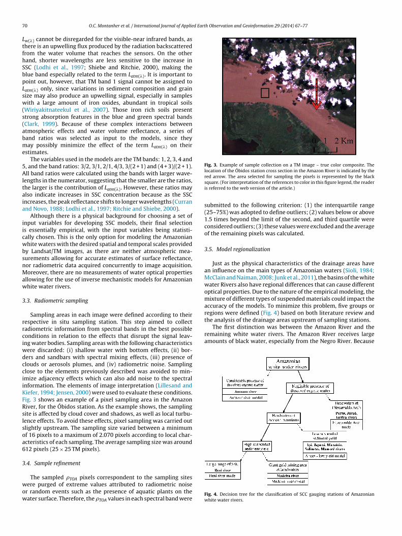
The first distinction was between the Amazon River and theremaining white water rivers. The Amazon River receives largeamounts of black water, especially from the Negro River. Because

0 O.C. Montanher et al. / International Journal of Applie

w(�) cannot be disregarded for the visible-near infrared bands, ashere is an upwelling flux produced by the radiation backscatteredrom the water volume that reaches the sensors. On the otherand, shorter wavelengths are less sensitive to the increase inSC (Lodhi et al., 1997; Shiebe and Ritchie, 2000), making thelue band especially related to the term Latm(�). It is important tooint out, however, that TM band 1 signal cannot be assigned toatm(�) only, since variations in sediment composition and grainize may also produce an upwelling signal, especially in samplesith a large amount of iron oxides, abundant in tropical soils

Wiriyakitnateekul et al., 2007). Those iron rich soils presenttrong absorption features in the blue and green spectral bandsClark, 1999). Because of these complex interactions betweentmospheric effects and water volume reflectance, a series ofand ratios was selected as input to the models, since theyay possibly minimize the effect of the term Latm(�) on their

stimates.The variables used in the models are the TM bands: 1, 2, 3, 4 and

, and the band ratios: 3/2, 3/1, 2/1, 4/3, 3/(2 + 1) and (4 + 3)/(2 + 1).ll band ratios were calculated using the bands with larger wave-

engths in the numerator, suggesting that the smaller are the ratios,he larger is the contribution of Latm(�). However, these ratios maylso indicate increases in SSC concentration because as the SSCncreases, the peak reflectance shifts to longer wavelengths (Currannd Novo, 1988; Lodhi et al., 1997; Ritchie and Shiebe, 2000).

Although there is a physical background for choosing a set ofnput variables for developing SSC models, their final selections essentially empirical, with the input variables being statisti-ally chosen. This is the only option for modeling the Amazonianhite waters with the desired spatial and temporal scales provided

y Landsat/TM images, as there are neither atmospheric mea-urements allowing for accurate estimates of surface reflectance,or radiometric data acquired concurrently to image acquisition.oreover, there are no measurements of water optical properties

llowing for the use of inverse mechanistic models for Amazonianhite water rivers.

.3. Radiometric sampling

Sampling areas in each image were defined according to theirespective in situ sampling station. This step aimed to collectadiometric information from spectral bands in the best possibleonditions in relation to the effects that disrupt the signal leav-ng water bodies. Sampling areas with the following characteristics

ere discarded: (i) shallow water with bottom effects, (ii) bor-ers and sandbars with spectral mixing effects, (iii) presence oflouds or aerosols plumes, and (iv) radiometric noise. Samplinglose to the elements previously described was avoided to min-mize adjacency effects which can also add noise to the spectralnformation. The elements of image interpretation (Lillesand andiefer, 1994; Jensen, 2000) were used to evaluate these conditions.ig. 3 shows an example of a pixel sampling area in the Amazoniver, for the Óbidos station. As the example shows, the samplingite is affected by cloud cover and shadows, as well as local turbu-ence effects. To avoid these effects, pixel sampling was carried outlightly upstream. The sampling size varied between a minimumf 16 pixels to a maximum of 2.070 pixels according to local char-cteristics of each sampling. The average sampling size was around12 pixels (25 × 25 TM pixels).

.4. Sample refinement

The sampled �TOA pixels correspondent to the sampling sitesere purged of extreme values attributed to radiometric noise

r random events such as the presence of aquatic plants on theater surface. Therefore, the �TOA values in each spectral band were

red arrow. The area selected for sampling the pixels is represented by the blacksquare. (For interpretation of the references to color in this figure legend, the readeris referred to the web version of the article.)

submitted to the following criterion: (1) the interquartile range(25–75%) was adopted to define outliers; (2) values below or above1.5 times beyond the limit of the second, and third quartile wereconsidered outliers; (3) these values were excluded and the averageof the remaining pixels was calculated.

3.5. Model regionalization

Just as the physical characteristics of the drainage areas havean influence on the main types of Amazonian waters (Sioli, 1984;McClain and Naiman, 2008; Junk et al., 2011), the basins of the whitewater Rivers also have regional differences that can cause differentoptical properties. Due to the nature of the empirical modeling, themixture of different types of suspended materials could impact theaccuracy of the models. To minimize this problem, five groups orregions were defined (Fig. 4) based on both literature review andthe analysis of the drainage areas upstream of sampling stations.

Fig. 4. Decision tree for the classification of SCC gauging stations of Amazonianwhite water rivers.

d Earth Observation and Geoinformation 29 (2014) 67–77 71

daR

bFtTtpgi

twtiasiebcaatD

netbu

yBtTlb

Table 1Regional model descriptive SSC (mg l−1) metrics. � and � are, respectively, averageand standard deviation of SSC values.

Model/region � � Minimum–maximum

Andes – low yield 136.85 111.13 0–728.4Madeira River 230.17 205.79 0.39–881.02Beni River 997.28 1103.11 28.3–3561.72

F(

O.C. Montanher et al. / International Journal of Applie

issolved organic materials have high absorption coefficientscross the visible spectrum, the reflectance values in the Amazoniver are lower relative to the rest of the white water rivers.

The rivers with low amounts of dissolved organic material coulde distinguished by the location of their headwaters: Andes anditzcarraldo Arch. Despite the high sediment yield in both headwa-er regions, they are located in very different geological settings.he Fitzcarraldo Arch region is dominated by tertiary sedimentaryerrains (Latrubesse et al., 2005) while the Andes are mainly com-osed of metamorphic and igneous rocks of crust. This difference ineological setting is assumed to be responsible for the differencesn the mineralogical composition of sediments.

Among the rivers with headwaters in the Andes, there werewo distinct groups: one with high sediment yield, and one otherith lower sediment yield. The criteria adopted for the defini-

ion of these two groups were relief amplitude and precipitationn the drainage areas. The group of high sediment yield includesreas of large relief amplitude and high precipitation rates. Bothouthern Peru Andes and Bolivian Andes have these character-stics in common. This region has fast rates of uplift (Wittmannt al., 2009) and large relief amplitudes (above 5000 m), which com-ined with the predominant lithology and basin average slopes,ause high rates of sediment production (Aalto et al., 2006). Inddition to the geological and topographical characteristics, therere extreme events of orographic precipitation in this region (upo about 6000 mm/year), highly concentrated in the months ofecember, January and February (Espinoza Villar et al., 2010).

The region of lower sediment yield covers drainage areas to theorth and south of that of high sediment yield. These terrains haveither high precipitation rates but lower relief amplitudes, such ashe headwaters of the Ic á and Japurá rivers, or high relief amplitudeut lower annual precipitation such as the catchment basin of thepper Maranón River and part of Mamore River basin.

A final distinction was made in the group of high sedimentield, between the sampling stations located in Madeira River andeni River. There is a large area of gold mining in southern Peru

hat adds large amounts of sediment to the Madeira River station.he Beni River station does not register this process, but has theargest amplitude of SSC among all stations used in this study,eing the only station that lies within the limits of the Andean

ig. 5. Stations used for each regional model of SSC as a function of Landsat 5/TM radiom3) Madeira River; (4) Fitzcarraldo Arch; (5) Andes – low yield.

Amazon River 56.4 40.53 10.4–180.09Fitzcarraldo Arch 197.07 207.21 7–1280.99

chain. Therefore, samples collected at this station did not sustainstrong depositional processes that occur in the Beni River floodplain(Wittmann et al., 2009).

Each of the five independent data sets used as input to the mod-els had distinct values of SSC (Table 1). The river basins of eachregional model are shown in Fig. 5.

3.6. Regression analysis

For model development, single bands and band ratios were pre-dictor variables for estimating the SSC (response variable). �TOAvalues for TM bands 1–5 entered the models scaled as percent-ages (0–100%), and band ratios were simple ratios between thesevariables.

The first step in the analysis was the fitting of a global model,using the whole data set, followed by fitting of regional modelsusing the corresponding data subsets, which consequently had dif-ferent SSC amplitudes. As the relationship between reflectance andSSC tends toward as asymptote as concentration levels increase,SSC values were transformed to minimize non-linear effects onthe fitted models. Two types of transformation were used, selectedin each case according observed SSC amplitude: (i) natural loga-rithm (lnSSC) for large amplitudes (global model and Beni Riverstation, amplitude: 0–3561 mg l−1); and (ii) square-root transfor-mation (

√SSC) for smaller amplitudes (all remaining regionalized

datasets, amplitude: 0–1280 mg l−1). We opted for different trans-

formations on a case-by-case basis since major transformations inthe response variable may cause undesired effects, such as changesin variance levels and distribution of errors (Kutner et al., 2005).

etric response, and their respective river basins: (1) Amazon River; (2) Beni River;

72 O.C. Montanher et al. / International Journal of Applied Earth Observation and Geoinformation 29 (2014) 67–77

Fig. 6. Dispersion between observed and estimated SSC values from the global model (A). Dispersion between the actual values and the values derived from cross-validation(B).

Table 2Statistics of the global model for the estimation of SSC from Landsat 5/TM data, in Amazonian white water rivers. k is the number of predictor variables, � are the LOOCVestimation errors, with average � and standard deviation �.

2 2 −1 −1

fitstfuLe

taaSe

4

4

avrmi

(mpt

4

rmo

the atmosphere and the air/water interface have no relationshipwith SSC or any other material present in the water. Only the BeniRiver model did not include short wavelength bands (blue or green)but it included band 5 and a series of band ratios. These band ratios

Table 3Global model for the estimation of SSC (mg l−1) in Amazonian white water riversfrom Landsat 5/TM �TOA . All variables have p-value < 0.00001. Result in natural log-arithm (lnSSC).

Coefficient Value

Intercept −14.21(B4 + B3)/(B2 + B1) 9.55B3/B1 −16.73B5 −0.32B2/B1 16.06B3/B2 12.24

Table 4Regional model for the estimation of SSC (mg l−1) in the Andes – low yield usingLandsat 5/TM �TOA . Result in square-root (

√SSC).

Coefficient Value p-Value

Intercept −19.391 0.0001B2 −6.489 <0.0001B3 7.114 <0.0001B5 −1.949 <0.0001

R R LOOCV N k

0.76 0.73 504 5

Once the variables were transformed, the models were initiallytted using all eleven variables (bands and band ratios) as predic-ors. However, as some variables might be redundant, a forwardtepwise regression (based on F-tests) was applied to determinehe optimal model structures. Once the best models were obtainedor each dataset, the predictive power of the models was simulatedsing the Leave-one-out cross validation technique (LOOCV). EachOOCV simulation produced a distribution of model predictionrror, which were summarized by its mean and standard deviation.

To compare the accuracy between global and regional models,he estimation errors of all five regional models were pooled into

single group (“regional models”). Root mean square error (RMSE)nd the Nash–Sutcliffe (E) model efficiency coefficient (Nash andutcliffe, 1970) were computed, and scatter plots of the estimationrrors for the two groups were also produced.

. Results and discussion

.1. Global model

The distribution of actual SSC against estimated SSC (Fig. 6A) had linear trend which was statistically significant (Table 2). Cross-alidation statistics showed that SSC estimates were very similar,egardless of the data set used in the development and testing of theodel (Fig. 6B). The model, however, has high variance, resulting

n high average errors of SSC estimates and standard deviation.Five variables were used for the global model, all significant

Table 3). The band ratios were extremely important when theodeling was carried out with the entire sampling set. Among the

ure spectral bands, only band 5 was selected for the model, withhe same degree of significance as the other variables in the model.

.2. Regional models

There was a wide variety of predictor variables selected by theegional models (Tables 4–8). Note that band 5 was selected in allodels, with a negative coefficient. The band of shorter wavelength

f four of the models had negative coefficients (in three cases, band

�: � (mg l ) �: � (mg l ) p-Value

99.32 266.21 <0.00001

2, and in one case, band 1). This model structure deals with the sig-nals from both the air/water interface and atmospheric scattering.

The atmospheric effects are larger at shorter wavelengths, andwater can be considered a dark object in the spectral range ofshortwave infrared, as that the signal ascending from the water isdue to specular reflection from the air/water interface. Because thecoefficients were negative, the larger the signals of band 5 and ofshorter wavelength bands for each model, the lower the estimatesof SSC, all other variables remaining constant. The behavior of thismodel has physical significance because the signals deriving from

B3/B1 −145.370 <0.0001B2/B1 112.236 <0.0001B4/B3 −25.970 0.0014(B4 + B3)/(B2 + B1) 92.354 <0.0001

O.C. Montanher et al. / International Journal of Applied Earth Observation and Geoinformation 29 (2014) 67–77 73

Fig. 7. Dispersion between actual values and the values estimated by regional models: Madeira River (a); Amazon River (b); Fitzcarraldo Arch (c); Andes – low yield (d); andBeni River (e).

74 O.C. Montanher et al. / International Journal of Applied Earth Observation and Geoinformation 29 (2014) 67–77

Table 5Regional model for the estimation of SSC (mg l−1) in the Madeira River using Landsat5/TM �TOA . Result in square-root (

√SSC).

Coefficient Value p-Value

Intercept −105.377 0.011B1 −7.933 0.0007B2 6.794 0.0031B5 −2.192 <0.0001B3/B2 179.462 <0.0001B3/B1 −164.636 <0.0001

mbo

lh

Table 6Regional model for the estimation of SSC (mg l−1) in the Beni River using Landsat5/TM �TOA . Result in natural logarithm (lnSSC).

Coefficient Value p-Value

Intercept −50.050 0.0006B5 −0.313 0.0211B3/B2 150.078 <0.0001B2/B1 57.720 0.0002B4/B3 −16.534 0.0003B3/(B2 + B1) −355.599 <0.0001

Fa

B2/B1 91.070 0.0331B4/B3 45.367 <0.0001

ay also be normalizing atmospheric effects, but the interactionsecome more complex, making difficult the physical interpretation

f this model.

Similar to the global model, the regional models had a consistentinear trend (Fig. 7). These models were statistically significant andad good cross-validation results (Table 9).

ig. 8. Dispersion between observed and estimated values of suspended sediment concennd B) and up to 800 mg l−1, for better observation of errors at lower levels (C and D).

(B4 + B3)/(B2 + B1) 44.306 <0.0001

Given the observed model structures, we believe that theycan be applied to other images that were not used in modeldevelopment, since atmospheric and air/water interface effects

are minimized. Regarding the remaining errors in the models, thisstudy hypothesizes that their main sources are the radiometric res-olution of Landsat 5/TM, and differences in sediment composition

tration, by the regional models and the global model for the entire range of SSC (A

O.C. Montanher et al. / International Journal of Applied Earth Observation and Geoinformation 29 (2014) 67–77 75

Table 7Regional model for the estimation of SSC (mg l−1) in the Fitzcarraldo Arch usingLandsat 5/TM �TOA . Result in square-root (

√SSC).

Coefficient Value p-Value

Intercept −74.007 0.0678B2 −2.278 0.022B3 3.024 0.0007B5 −1.278 0.0044B3/B2 183.804 0.0365B2/B1 99.846 0.0203B3/(B2 + B1) −462.418 0.0119(B4 + B3)/(B2 + B1) 29.788 <0.0001

Table 8Regional model for the estimation of SSC (mg l−1) in the Amazon River using Landsat5/TM �TOA . Result in square-root (

√SSC).

Coefficient Value p-Value

Intercept 25.264 0.0075B2 −2.623 0.001B3 1.876 0.0368B4 1.726 <0.0001B5 −0.922 <0.0001B3/B1 27.904 0.0181

afot1da

atioeed

stGs

4

r(ifri

large number of images.

TSL

B4/B3 −11.789 0.0130B3/(B2 + B1) −81.236 0.0464

nd grain size distribution between images of different dates. Inact, these characteristics strongly influence the optical propertiesf the aquatic environment, including the shape and intensity ofhe reflectance spectrum (Novo et al., 1989; Han and Rundquist,996; Lodhi et al., 1997). Seasonal variation in sediment type canecrease the predictive ability of empirical models even when theyre developed regionally, according to drainage basin environment.

The time difference between satellite and in situ measurementslso could be a source of error. The ideal condition is the concomi-ance between databases, but this makes the model generationmpossible, because most of the data are not concurrent to satelliteverpasses and lack information about sampling time. Therefore,ven though the maximum interval of nine days might inducerrors in the models, it is necessary for increasing the amount ofata for modeling.

Additionally, one or more days of difference between data acqui-ition are certainly problematic for small drainage basins, subjecto short time changes in hydrologic regime and sediment yield.iant fluvial basins, like those under study, have hydrological andediment transport variations in a much greater period, e.g. weeks.

.3. Comparison of models (global and regional approaches)

The estimates provided by the regional models are more accu-ate than those of the global models, especially for higher SSCFig. 8). Larger accuracy differences are noticeable when compar-ng RSME and Nash–Sutcliffe coefficients, of 283.6 mg l−1 and 0.47

or the global model and 113.7 mg l−1 and 0.91 for regional models,espectively. In both approaches, the errors increased with increas-ng levels of SSC, but with smaller dispersion in the regional models.

able 9tatistics of the regional models for the estimation of SSC from Landsat 5 TM data, in AmOOCV errors of estimation. All models have p-value < 0.00001.

Model Adjusted R2 R2 LOOCV

Andes – low yield 0.77 0.72

Madeira River 0.84 0.81

Beni River 0.89 0.79

Amazon River 0.88 0.86

Fitzcarraldo Arch 0.82 0.78

Fig. 9. Dispersion between average errors and standard deviation (SSC) of regionalmodels, and maximum levels captured by the models. Both average errors andstandard deviation increase exponentially with the increase in SSC.

This trend is also observed when assessing regional model errorsas function of the SSC extreme concentrations (Fig. 9).

There was a relationship between estimate errors and SSC con-centration levels. As SSC increased, the growth rate of backscatteredwater signals decreased. The function that expresses this relation-ship is logarithmic (Curran and Novo, 1988; Lodhi et al., 1997;Shiebe and Ritchie, 2000): as the levels of SSC increased, thebackscattered signal not detected, due to low radiometric resolu-tion of the TM sensor, became increasingly important, explaininghigher estimate errors.

4.4. Recommendations for model application

The application of these models is not recommended for cir-cumstances requiring a highly accurate estimate of SSC, e.g. withacceptable errors below 10 mg l−1. Still, the use of the present mod-els may allow an unprecedented increase in SSC data availability forAmazonian white water rivers, in both spatial and temporal scales.The long historical series of LANDSAT 5/TM images can thereforebe used to assess environmental changes in the basins of Amazo-nian white water rivers. Changes in the hydrologic regime inducedby land use and land cover changes, or by variations in precipita-tion regime, and their relationships to sediment production in theAmazon Basin can be better evaluated with the use of these mod-els. Also, as the input for these models is the top of the atmospherereflectance, which is easily calculated (Chander et al., 2009), theirapplication is easily operationalized and can be performed on a

Finally, the availability of imagery from the recently launchedLandsat 8/OLI (LDCM) could allow for continued monitoring of SSClevels in Amazonian white water rivers, with a larger accuracy than

azonian white water rivers. k is the number of predictor variables and � are the

N k �: � (mg l−1) �: � (mg l−1)

112 7 39.55 37.07168 7 59.66 63.68

34 6 330.2 359.783 7 10.12 7.81

107 7 67.98 73.03

7 d Eart

tr

5

replsn

aLeiassopa

A

sftcot5gct

A

TI

6 O.C. Montanher et al. / International Journal of Applie

he present models, given the enhanced spectral and radiometricesolution provided by OLI instrument (Irons et al., 2012).

. Conclusions

The global model for estimating SSC in Amazonian white waterivers does not provide estimates as accurate as the regional mod-ls. Estimation errors increased with increasing levels of SSC. Theatterns of including SWIR and visible bands of shorter wave-

engths in the regional models, with negative coefficients, aretrong evidence that the models are capable of dealing with effectsot related with the suspended components in the water.

The model development reported here is one of the largestttempts to retrieve SSC information for large river systems, usingandsat imagery. The large amount of images used to fit the mod-ls (504) and estimate SSC means that this work would be almostmpracticable if images were to be commercially acquired. The freeccess to Landsat historical data allowed us to obtain a new per-pective on studies of suspended sediment transport in large riverystems, unknown until a few years ago. Using this database, andur models, new and promising possibilities for studies of the sus-ended sediment transport in large Amazonian white water riversre now available.

cknowledgements

This work would not be possible without the free availability ofatellite images and in situ data, and the authors are grateful for theree distribution policy of Landsat images by NASA and INPE, and forhe distribution of in situ data by ANA and Hybam. We thank Mauri-io Carvalho Mathias de Paulo for assistance with the automationf image calibration. Otávio Cristiano Montanher thanks CAPES forhe scholarship supporting his master’s degree, and CNPq grant51034/2011-4 for the PCI scholarship. Evlyn Novo thanks FAPESPrant 2011/23594-8 and CNPq grant 550373/2010-1 for the finan-ial support of the research conducted in the Amazon. Thiago Silvahanks FAPESP grant 2010/11269-2 for the postdoctoral support.

ppendix A.

able A1n situ SSC sampling stations used in the model development.

In situ stations names Identification River Country/source

Ipiranga Velho 11450000 Ic á Brazil/ANAVila Bittencourt 12845000 Japurá Brazil/ANAFeijó 12650000 Envira Brazil/ANACruzeiro do Sul 12500000 Juruá Brazil/ANAEirunepé 12550000 Juruá Brazil/ANAGavião 12840000 Juruá Brazil/ANAArumã-Jusante 13962000 Purus Brazil/ANALábrea 13870000 Purus Brazil/ANASeringal Fortaleza 13750000 Purus Brazil/ANASeringal da Caridade 13410000 Purus Brazil/ANAAbunã 15320002 Madeira Brazil/ANAPorto Velho 15400000 Madeira Brazil/ANA/HYBAMHumaitá 15630000 Madeira Brazil/ANAManicoré 15700000 Madeira Brazil/ANAFazenda Vista Alegre 15860000 Madeira Brazil/ANA/HYBAMGuarajá-Mirim 15250000 Mamoré Brazil/ANATeresina 11200000 Solimões Brazil/ANASão Paulo de Olivenc a 11400000 Solimões Brazil/ANAItapéua 13150000 Solimões Brazil/ANA

Manacapuru 14100000 Solimões Brazil/ANAÓbidos 17050001 Amazon Brazil/ANA/HYBAMBorja 10064000 Maranón Peru/HYBAMRurrenabaque 15275100 Beni Bolivia/HYBAM

h Observation and Geoinformation 29 (2014) 67–77

References

Aalto, R., Dunne, T., Guyot, J.L., 2006. Geomorphic controls on Andean denudationdates. Journal of Geology 114, 85–99.

Aranuvachapun, S., Walling, D.E., 1988. Landsat-MSS radiance as a measure of sus-pended sediment in the lower Yellow River (Hwang Ho). Remote Sensing ofEnvironment 25, 145–165.

Baby, P., Guyot, J.L., Hérail, G., 2009. Tectonic control of erosion and sed-imentation in the Amazon Basin of Bolivia. Hydrological Processes 23,3225–3229.

Chander, G., Markham, B.L., Helder, D.L., 2009. Summary of current radiometric cal-ibration coefficients for Landsat MSS, TM, ETM+, and EO-1 ALI sensors. RemoteSensing of Environment 113, 893–903.

Clark, R.N., 1999. Spectroscopy of rocks and minerals, and principles of spectroscopy.In: Rencz, A.N. (Ed.), Manual of Remote Sensing, Volume 3, Remote Sensing forthe Earth Sciences. John Wiley and Sons, New York, pp. 3–58.

Costa, M.P.F., Novo, E.M.L.M., Thelmer, K., 2012. Spatial and temporal variability oflight attenuation in large Rivers of the Amazon. Hydrobiologia 698, 1–22.

Curran, P.J., Novo, E.M.L.M., 1988. The relationship between suspended sedimentconcentration and remotely sensed spectral radiance: a review. Journal ofCoastal Research 4, 351–368.

Dekker, A.G., Voss, R.J., Peters, S.W.M., 2002. Analytical algorithms for lake water TSMestimation for retrospective analysis of TM and SPOT sensor data. InternationalJournal of Remote Sensing 23, 15–35.

Espinoza Villar, J.C., Ronchail, J., Lavado, W., Carranza, J., Cochonneau, G., Oliveira,E., Pombosa, R., Vauchel, P., Guyot, J.L., 2010. Variabilidad espacio-temporal delas lluvias em la cuenca amazônica y su relación con la variabilidad hidrológicaregional. Un enfoque particular sobre la región andina. Revista Peruana Geo-atmosférica 2, 99–130.

Espinoza Villar, R., Martinez, J.M., Guyot, J.L., Fraizy, P., Armijos, E., Crave, A., Bazán,H., Vauchel, P., Lavado, W., 2012. The integration of field measurements andsatellite observations to determine river solid loads in poorly monitored basins.Journal of Hydrology 444, 221–228.

Espinoza Villar, R., Martinez, J.M., Texier, M.L., Guyot, J.L., Fraizy, P., Meneses, P.R.,Oliveira, E., 2013. A study of sediment transport in the Madeira River, Brazil,using MODIS remote-sensing images. Journal of South American Earth Sciences44, 45–54.

Espurt, N., Baby, P., Brusset, S., Roddaz, M., Hermoza, R.V., Antoine, P.O., Salas-Gismondi, R., Bolãnos, R., 2007. How does the Nazca Ridge subduction influencethe modern Amazonian foreland basin? Geology 35, 515–518.

Han, L., Rundquist, D.C., 1996. Spectra characterization of suspended sediments gen-erated from two texture classes of clay soil. International Journal of RemoteSensing 17, 643–649.

Holben, B.N., Eck, T.F., Slutsker, I., Tanré, D., Buis, J.P., Setzer, A., Vermote, E., Rea-gan, J.A., Kaufman, Y., Nakajima, T., Lavenu, F., Jankowiak, I., Smirnov, A., 1998.AERONET – a federated instrument network and data archive for aerosol char-acterization. Remote Sensing of Environment 66, 1–16.

Irons, J.R., Dwyer, J.L., Barsi, J.A., 2012. The next Landsat satellite: the Landsat datacontinuity mission. Remote Sensing of Environment 122, 11–21.

Islam, A., Gao, J., Ahmad, W., Neil, D., Bell, P., 2004. A composite DOP approach toexcluding bottom reflectance in mapping water parameters of shallow coastalzones from TM imagery. Remote Sensing of Environment 92, 40–51.

Jensen, J.R., 2000. Remote Sensing of the Environment: An Earth Resource Perspec-tive. Prentice Hall, Upper Saddle River.

Junk, W., Piedade, M.T.F., Schöngart, J., Cohn-Haft, M., Adeney, J.M., Wittmann, F.,2011. A classification of major naturally-occurring Amazonian lowland wet-lands. Wetlands 31, 623–640.

Kerr, S.J., 1995. Silt, turbidity and suspended sediments in the aquatic environment:an annotated bibliography and literature review. Technical Report TR-008.Ontario Ministry of Natural Resources, Southern Region Science & TechnologyTransfer Unit.

Khorram, S., 1985. Development of water quality models applicable throughout theentire San Francisco Bay and Delta. Photogrammetric Engineering & RemoteSensing 51, 53–62.

Kishino, M., Tanaka, A., Ishizaka, J., 2005. Retrieval of chlorophyll a, suspended solids,and colored dissolved organic matter in Tokyo Bay using ASTER data. RemoteSensing of Environment 99, 66–74.

Kutner, M.H., Nachtsheim, C.J., Neter, J., Li, W., 2005. Applied Linear Statistical Mod-els, fifth ed. McGraw-Hill, Boston.

Latrubesse, E., Stevaux, J.C., Sinha, R., 2005. Tropical rivers. Geomorphology 70,137–206.

Lillesand, T.M., Kiefer, R.W., 1994. Remote sensing and image interpretation, thirded. John Wiley & Sons, New York.

Lodhi, M.A., Rundquist, D.C., Han, L., Kuzila, M.S., 1997. The potential for remotesensing of loess soils suspended in surface waters. Journal of the American WaterResources Association 33, 111–117.

Loveland, T.R., Dwyer, J.L., 2012. Landsat: building a strong future. Remote Sensingof Environment 122, 22–29.

Mangiarotti, S., Martinez, J.M., Bonnet, M.P., Buarque, D.C., Filizola, N., Mazzega,P., 2013. Discharge and suspended sediment flux estimated along the main-stream of the Amazon and the Madeira Rivers (from in situ and MODIS Satellite

Data). International Journal of Applied Earth Observation and Geoinformation21, 341–355.

Markhan, B.L., Barker, J.L., 1986. Landsat MSS and TM Post-Calibration DynamicRanges, Exoatmospheric Reflectances and At-Satellite Temperature. EOSATLandsat Technical Notes, n. 1, p. 8, ago.

d Eart

M

M

M

M

M

M

M

N

N

N

P

R

R

R

O.C. Montanher et al. / International Journal of Applie

arkham, B.L., Helder, D.L., 2012. Forty-year calibrated record of earth-reflectedradiance from Landsat: a review. Remote Sensing of Environment 122, 30–40.

artinez, J.M., Guyot, J.L., Filizola, N., Sondag, F., 2009. Increase in suspended sed-iment discharge of the Amazon River assessed by monitoring network andsatellite data. Catena 79, 257–264.

atthews, M.W., Bernard, S., Winter, K., 2010. Remote sensing of cyanobacteria-dominant algal blooms and water quality parameters in Zeekoevlei, asmall hypertrophic lake, using MERIS. Remote Sensing of Environment 114,2070–2087.

cClain, M.E., Naiman, R.J., 2008. Andean influences on the biogeochemistry andecology of the Amazon River. BioScience 58, 325–338.

ertes, L.A.K., 1994. Rates of flood-plain sedimentation on the central Amazon River.Geology 22, 171–174.

ertes, L.A.K., 2002. Remote sensing of riverine landscapes. Freshwater Biology 47,799–816.

ertes, L.A.K., Smith, M.O., Adams, J.B., 1993. Estimating suspended sediment con-centrations in surface waters of the Amazon River wetlands from Landsatimages. Remote Sensing of Environment 43, 281–301.

anson, G.C., Croke, J.C., 1992. A genetic classification of floodplains. Geomorphology4, 459–486.

ash, J.E., Sutcliffe, J.V., 1970. River flow forecasting through conceptual models,Part-I: a discussion of principles. Journal of Hydrology 10, 282–290.

ovo, E.M.L.M., Hanson, J.D., Curran, P.J., 1989. The effect of sediment type on therelationship between reflectance and suspended sediment concentration. Inter-national Journal of Remote Sensing 10, 1283–1289.

ierce, A.R., King, S.L., 2008. Spatial dynamics of overbank sedimentation in flood-plain systems. Geomorphology 100, 256–268.

äsänen, M.E., Salo, J.S., Kalliola, R.J., 1987. Fluvial perturbance in the westernAmazon basin: regulation by long-term sub-Andean tectonics. Science 238,1398–1401.

itchie, J.C., Cooper, C.M., Yongqing, J., 1987. Using Landsat Multispectral Scan-

ner data to estimate suspended sediments in Moon Lake, Mississippi. RemoteSensing of Environment 23, 65–81.

itchie, J.C., Shiebe, F.R., 2000. Water quality. In: Shultz, G.A., Engman, E.T(Eds.), Remote Sensing in Hydrology and Water Management. Springer,pp. 287–303.

h Observation and Geoinformation 29 (2014) 67–77 77

Sioli, H., 1984. The Amazon: Limnology and Landscape Ecology of a Mighty TropicalRiver and Its Basin. W. Junk, Dordrecht (Netherlands).

Tebbs, E.J., Remedios, J.J., Harper, D.M., 2013. Remote sensing of chlorophyll a asa measure of cyanobacterial biomass in Lake Bogoria, a hypertrophic, saline-alkaline, flamingo lake, using Landsat ETM+. Remote Sensing of Environment135, 92–106.

Thornton, K.W., 1990. Perspectives on reservoir limnology. In: Thornton, K.W., Kim-mel, B.L., Payne, F.E. (Eds.), Reservoir Limnology: Ecological Perspectives. Wiley,New York.

Thornton, K.W., Kennedy, R.H., Carrol, J.H., Walker, W.W., Gunkel, R.C., Ashby, S.,1981. Reservoir sedimentation and water quality: a heuristic model. In: Ste-fen, H.G. (Ed.), Proceedings of the Symposium on Surface Water Impoundments.American Society of Civil Engineers, New York, pp. 654–661.

Walling, D.E., He, Q., 1998. The spatial variability of overbank sedimentation on riverfloodplains. Geomorphology 24, 209–223.

Wang, M., 2007. Remote sensing of the ocean contributions from ultraviolet to near-infrared using the shortwave infrared bands: simulations. Applied Optics 46,1535–1547.

Wang, J.J., Lu, X.X., 2010. Estimation of suspended sediment concentrations usingTerra MODIS: an example from the Lower Yangtze River, China. Science of theTotal Environment 408, 1131–1138.

Wang, J.J., Lu, X.X., Liew, S.C., Zhou, Y., 2009. Retrieval of suspended sediment concen-trations in large turbid rivers using Landsat ETM+: an example from the YangtzeRiver, China. Earth Surface Processes and Landforms 34, 1082–1092.

Wetzel, R.G., 2001. Limnology: Lake and River Ecosystems. Academic Press, SanDiego.

Wiriyakitnateekul, W., Suddhiprakarn, A., Kheoruenromne, I., Smirk, M.N., Gilkes,R.J., 2007. Iron oxides in tropical soils on various parent materials. Clay Minerals42, 437–451.

Wittmann, H., Von Blanckenburg, F., Guyot, J.L., Maurice, L., Kubik, P.W., 2009. Fromsource to sink: preserving the cosmogenic 10Be-derived denudation rate signal

of the Bolivian Andes in sediment of the Beni and Mamoré foreland basins. Earthand Planetary Science Letters 288, 463–474.

Wulder, M.A., Masek, J.G., Cohen, W.B., Loveland, T.R., Woodcock, C.E., 2012. Openingthe archive: how free data has enabled the science and monitoring promise ofLandsat. Remote Sensing of Environment 122, 2–10.