This article was downloaded by: [University of Saskatchewan Library]On: 24 September 2012, At: 00:27Publisher: RoutledgeInforma Ltd Registered in England and Wales Registered Number: 1072954 Registered office: MortimerHouse, 37-41 Mortimer Street, London W1T 3JH, UK

Quantitative FinancePublication details, including instructions for authors and subscription information:http://www.tandfonline.com/loi/rquf20

Empirical modelling of contagion: a review ofmethodologiesMardi Dungey a b , Renée Fry a , Brenda González-Hermosillo c & Vance L. Martin da Economics Division, Research School of Pacific and Asian Studies, HC Coombs Building,Australian National University, ACT 0200, Australiab CERF, Cambridge University, Cambridge, UKc International Monetary Fundd University of Melbourne, Melbourne, Australiae Economics Division, Research School of Pacific and Asian Studies, HC Coombs Building,Australian National University, ACT 0200, Australia E-mail:

Version of record first published: 18 Feb 2007.

To cite this article: Mardi Dungey , Renée Fry, Brenda González-Hermosillo & Vance L. Martin (2005): Empirical modellingof contagion: a review of methodologies, Quantitative Finance, 5:1, 9-24

To link to this article: http://dx.doi.org/10.1080/14697680500142045

PLEASE SCROLL DOWN FOR ARTICLE

Full terms and conditions of use: http://www.tandfonline.com/page/terms-and-conditions

This article may be used for research, teaching, and private study purposes. Any substantial or systematicreproduction, redistribution, reselling, loan, sub-licensing, systematic supply, or distribution in any form toanyone is expressly forbidden.

The publisher does not give any warranty express or implied or make any representation that the contentswill be complete or accurate or up to date. The accuracy of any instructions, formulae, and drug dosesshould be independently verified with primary sources. The publisher shall not be liable for any loss, actions,claims, proceedings, demand, or costs or damages whatsoever or howsoever caused arising directly orindirectly in connection with or arising out of the use of this material.

Quantitative Finance, Vol. 5, No. 1, February 2005, 9–24

Empirical modelling of contagion:

a review of methodologies

MARDI DUNGEY*yz, RENEE FRYy,BRENDA GONZALEZ-HERMOSILLO§ and VANCE L. MARTIN�

yEconomics Division, Research School of Pacific and Asian Studies,HC Coombs Building, Australian National University, ACT 0200, Australia

zCERF, Cambridge University, Cambridge, UK§International Monetary Fund

�University of Melbourne, Melbourne, Australia

(Received 16 October 2003; in final form 5 February 2005)

1. Introduction

There is now a reasonably large body of empirical worktesting for the existence of contagion during financialcrises. A range of different methodologies are in use,making it difficult to assess the evidence for and againstcontagion, and particularly its significance in transmittingcrises between countries. The origins of current empiricalstudies of contagion stem from Sharpe (1964) and Grubeland Fadner (1971), and more recently from King andWadhwani (1990), Engle et al. (1990) and Bekaert andHodrick (1992).k

The aim of the present paper is to provide a unifyingframework to highlight the key similarities and differ-ences between the various approaches. For an overviewof the literature see Dornbusch et al. (2000) and Pericoliand Sbracia (2003). The proposed framework is based ona latent factor structure which forms the basis of themodels of Dungey and Martin (2001), Corsetti et al.(2001, 2003) and Bekaert et al. (2005). This frameworkis used to compare directly the correlation analysisapproach popularized in this literature by Forbes andRigobon (2002), the VAR approach of Favero andGiavazzi (2002), the probability model of Eichengreenet al. (1995, 1996) and the co-exceedance approach ofBae et al. (2003).

An important outcome of this paper is that differencesin the definitions used to test for contagion are minor

and under certain conditions are even equivalent. In par-ticular, all definitions are interpreted as working fromthe same model, with the differences stemming fromthe amount of information used in the data to detectcontagion. Interpreting the approaches in this wayprovides a natural ordering of models across the infor-mation spectrum with some models representing fullinformation methods and others representing partialinformation methods.

The paper proceeds as follows. In section 2 a frame-work is developed to model the interdependence betweenasset returns in a non-crisis environment. This frameworkis augmented in section 3 to give a model which includesan avenue for contagion during a crisis. The relationshipbetween this model and the bivariate correlation testsfor contagion of Forbes and Rigobon is discussed insection 4. This section also includes a number of exten-sions of the original Forbes and Rigobon approach, aswell as its relationship with the approaches of Faveroand Giavazzi (2002), Eichengreen et al. (1995, 1996)and Bae et al. (2003). An empirical example comparingthe various contagion tests is contained in section 5.The results show that the Forbes and Rigobon adjustedcorrelation test is a conservative test, whereas the conta-gion test of Favero and Giavazzi tends to reject the null ofno contagion too easily. The remaining tests investigatedyield results falling within these two extremes. Concludingcomments are given in section 6 together with a number

*Corresponding author. Email: m.dungey@cerf.cam.ac.ukkAs this paper focuses on empirical models of contagion it does not discuss the corresponding theoretical literature and moregenerally the literature on financial crises. For examples of theoretical models of contagion see Allen and Gale (2000), Calvo andMendoza (2000), Kyle and Xiong (2001), Chue (2002), Kiyotaki and Moore (2002) and Kodres and Pritsker (2002). The literatureon financial crises is overviewed in Flood and Marion (1998).

Quantitative FinanceISSN 1469–7688 print/ISSN 1469–7696 online # 2005 Taylor & Francis Group Ltd

http://www.tandf.co.uk/journalsDOI: 10.1080/14697680500142045

Dow

nloa

ded

by [

Uni

vers

ity o

f Sa

skat

chew

an L

ibra

ry]

at 0

0:27

24

Sept

embe

r 20

12

of suggestions for future research that encompass boththeoretical and empirical issues.

2. A model of interdependence

Before developing a model of contagion, a model ofinterdependence of asset markets during non-crisisperiods is specified as a latent factor model of assetreturns. The model has its origins in the factor models infinance based on arbitrage pricing theory for example,where asset returns are determined by a set of commonfactors representing non-diversifiable risk and a set ofidiosyncratic factors representing diversifiable risk(Sharpe 1964, Solnik 1974). Similar latent factor modelsof contagion are used by Corsetti et al. (2003, 2001),Dungey and Martin (2001), Dungey et al. (2005b),Forbes and Rigobon (2002) and Bekaert et al. (2005).

To simplify the analysis, the number of assets con-sidered is three. Extending the model to N assets orasset classes is straightforward. Let the returns of threeassets during a non-crisis period be defined as

x1, t, x2, t, x3, t� �

: ð1Þ

All returns are assumed to have zero means. The returnscould be on currencies, or national equity markets, or acombination of currency and equity returns in a partic-ular country or across countries.y The following trivariatefactor model is assumed to summarize the dynamics ofthe three processes during a period of tranquility

xi, t ¼ �iwt þ �iui, t, i ¼ 1, 2, 3: ð2Þ

The variable wt represents common shocks that impactupon all asset returns with loadings �i: These shockscould represent financial shocks arising from changesto the risk aversion of international investors, or changesin world endowments (Mahieu and Schotman 1994,Cizeau et al. 2001, Rigobon 2003b). In general, wt repre-sents market fundamentals which determine the averagelevel of asset returns across international markets during‘normal’, that is, tranquil, times. This variable is com-monly referred to as a world factor, which may or maynot be observed.z For expositional purposes, the worldfactor is assumed to be a latent stochastic process withzero mean and unit variance

wt � 0, 1ð Þ: ð3Þ

The properties of this factor are extended below to cap-ture richer dynamics including both autocorrelation andtime-varying volatility. The terms ui, t in equation (2) areidiosyncratic factors that are unique to a specific assetmarket. The contribution of idiosyncratic shocks to thevolatility of asset returns is determined by the loadings

�i > 0: These factors are also assumed to be stochasticprocesses with zero mean and unit variance

ui, t � 0, 1ð Þ: ð4Þ

To complete the specification of the model, all factorsare assumed to be independent

E ui, tuj, t� �

¼ 0, 8i 6¼ j, ð5Þ

E ui, twt

� �¼ 0, 8i: ð6Þ

To highlight the interrelationships amongst the three assetreturns in (2) during a non-crisis period, the covariancesare given by

E xi, txj, t� �

¼ �i�j , 8i 6¼ j, ð7Þ

whilst the variances are

E x2i, t� �

¼ �2i þ �2i , 8i: ð8Þ

Expression (7) shows that any dependence between assetreturns is solely the result of the influence of commonshocks arising from wt, which simultaneously impactupon all markets. Setting

�1 ¼ �2 ¼ �3 ¼ 0, ð9Þ

results in independent asset markets with all movementsdetermined by the idiosyncratic shocks, ui, t.§ The identi-fying assumption used by Mahieu and Schotman (1994)in a similar problem is to set �i�j to a constant value, L,for all i 6¼ j.

3. An empirical model of contagion

In this paper contagion is represented by the contem-poraneous transmission of local shocks to anothercountry or market after conditioning on common fac-tors that exist over a non-crisis period, given by wt inequation (2). This definition is consistent with that ofMasson (1999a, b, c), who decomposes shocks to assetmarkets into common spillovers, which result fromsome identifiable channel, and contagion. As shownbelow this definition is also consistent with that of otherapproaches, such as Forbes and Rigobon (2002), wherecontagion is represented by an increase in correlationduring periods of crisis.

The first model discussed is based on the factor struc-ture developed by Dungey et al. (2002, 2005b). Considerthe case of contagion from country 1 to country 2.The factor model in (2) is now augmented as follows

y1, t ¼ �1wt þ �1u1, t,

y2, t ¼ �2wt þ �2u2, t þ �u1, t,

y3, t ¼ �3wt þ �3u3, t, ð10Þ

ySee, for example, Granger et al. (2000), Hartmann et al. (2004) and Bekaert et al. (2005), who model the interactions between assetclasses.zThe model outlined here can be extended to allow for a richer set of factors, including observed fundamentals (Eichengreen et al.1995, 1996), trade linkages (Glick and Rose 1999, Pesaran and Pick 2003), financial flows (Van Rijckeghem and Weder 2001),geographical distance (Bayoumi et al. 2003) and Fama-French factors (Flood and Rose 2005).§Of course, just two of the restrictions in (7) are sufficient for independence of asset markets.

10 Survey

Dow

nloa

ded

by [

Uni

vers

ity o

f Sa

skat

chew

an L

ibra

ry]

at 0

0:27

24

Sept

embe

r 20

12

where the xi, t in (2) are replaced by yi, t to signifydemeaned asset returns during the crisis period. Theexpression for y2, t now contains a contagious trans-mission channel as represented by local shocks fromthe asset market in country 1, with its impact measuredby the parameter �. The fundamental aim of all empiricalmodels of contagion is to test the statistical significanceof the parameter �.y

3.1. Bivariate testing

Bivariate tests of contagion focus on changes in the vola-tility of pairs of asset returns. From (10), the covariancebetween the asset returns of countries 1 and 2 duringthe crisis is

E y1, ty2, t� �

¼ �1�2 þ ��1: ð11Þ

Comparing this expression with the covariance for thenon-crisis period in (7) shows that the change in thecovariance between the two periods is

E y1, ty2, t� �

� E x1, tx2, t� �

¼ ��1: ð12Þ

If � > 0, there is an increase in the covariance of assetreturns during the crisis period as �1 > 0 by assumption.This is usually the situation observed in crisis data.However, it is possible for � < 0, in which case there isa reduction in the covariance. Both situations are valid asboth represent evidence of contagion via the impact ofshocks in (10). Hence a test of contagion is given bytesting the restriction

� ¼ 0, ð13Þ

in the factor model in equation (10). This is the approachadopted by Dungey et al. (2002, 2003a, 2005b) andDungey and Martin (2004).z

An alternative way to construct a test of contagion isto use the volatility expression for y2, t, which is given by

E y22, t� �

¼ �22 þ �22 þ �2: ð14Þ

Comparing this expression with (8) shows that thechange in volatility over the two periods is solely attrib-uted to the presence of contagion

E y22, t� �

� E x22, t� �

¼ �2: ð15Þ

Thus, the contagion test based on (13) can be interpretedas a test of whether there is an increase in volatility.Expression (14) suggests that a useful description ofthe volatility of y2, t is to decompose the effects of shocksinto common, idiosyncratic and contagion respectivelyas follows

�22�22 þ �22 þ �2

,�22

�22 þ �22 þ �2,

�2

�22 þ �22 þ �2: ð16Þ

This decomposition provides a descriptive measure ofthe relative strength of contagion in contributing to thevolatility of returns during a crisis period. As before,the strength of contagion is determined by the parameter�, which can be tested formally.

3.2. Multivariate testing

The test for contagion presented so far is a test for con-tagion from country 1 to country 2. However, it is pos-sible to test for contagion in many directions providedthat there are sufficient moment conditions to identifythe unknown parameters. For example, (10) can beextended as

y1, t ¼ �1wt þ �1u1, t þ �1, 2u2, t þ �1, 3u3, t,

y2, t ¼ �2wt þ �2u2, t þ �2, 1u1, t þ �2, 3u3, t,

y3, t ¼ �3wt þ �3u3, t þ �3, 1u1, t þ �3, 2u2, t, ð17Þ

or more succinctly

yi, t ¼ �iwt þ �iui, t þX3

j¼ 1, j 6¼ i

�i, juj, t, i ¼ 1, 2, 3: ð18Þ

The theoretical variances and covariances are an exten-sion of the expressions given in (14) and (11) respectively.For example, the variance of the returns of country 1 is

E y21, t� �

¼ �21 þ �21 þ �21, 2 þ �2

1, 3, ð19Þ

whereas the covariance of asset returns between coun-tries 1 and 2 is

E y1, ty2, t� �

¼ �1�2 þ �1�2, 1 þ �2�1, 2 þ �1, 3�2, 3: ð20Þ

In this case there are 6 parameters, �i, j, controlling thestrength of contagion across all asset markets. This model,by itself, is unidentified as there are 12 unknown param-eters. However, by combining the empirical momentsof the variance–covariance matrix during the crisisperiod, 6 moments, with the empirical moments fromthe variance–covariance matrix of the non-crisis period,another 6 moments, gives 12 empirical moments in totalwhich can be used to estimate the 12 unknown parametersby the generalized method of moments (GMM).

A joint test of contagion, using the factor modelsin (2) and (17), can be achieved by comparing the objec-tive function from the unconstrained model, qu, withthe value obtained from estimating the constrainedmodel, qc, where the contagion parameters are set tozero. As the unconstrained model is just identified inthis case, qu ¼ 0, the test is simply a test that under thenull hypothesis of no contagion

H0 : qc ¼ 0, ð21Þ

which is distributed asymptotically as �2 with 6 degreesof freedom under the null. As before, the test of

yAn important assumption underlying (10) is that the common shock (wt) and idiosyncratic shocks (ui, t) have the same impactduring the crisis period as they have during the non-crisis period. This assumption of no structural break is discussed in section 3.3.zMost concern seems to centre on the case where � > 0, that is where contagion is associated with a rise in volatility. The existingtests can be characterized as testing the null hypothesis of � ¼ 0 against either a two-sided alternative or a one-sided alternative.

Survey 11

Dow

nloa

ded

by [

Uni

vers

ity o

f Sa

skat

chew

an L

ibra

ry]

at 0

0:27

24

Sept

embe

r 20

12

contagion can be interpreted as testing for changes inboth variances and covariances.

3.3. Structural breaks

The model given by equations (2) and (18) is based onthe assumption that the increase in volatility during thecrisis period is solely generated by contagion, that is,�i, j 6¼ 0, 8i, j. However, another scenario is that there isa general increase in volatility without any contagion;denoted as increased interdependence by Forbes andRigobon (2002). This would arise if either the world load-ings �ið Þ change, or idiosyncratic loadings �ið Þ change,or a combination of the two. The former would be repre-sentative of a general increase in volatility across allasset markets brought about, for example, by an increasein the risk aversion of international investors. The latterwould arise from increases in the shocks of (some) indi-vidual asset markets which are entirely specific to thosemarkets and thus independent of other asset markets.

To allow for structural breaks in the underlying rela-tionships the number of contagious linkages that canbe entertained needs to be restricted. In the case wherechanges in the idiosyncratic shocks are allowed across thesample periods in all N ¼ 3 asset markets, equation (18)becomes

yi, t ¼ �iwt þ �y, iui, t þX3

j¼ 1, j 6¼ i

�i, juj, t, ð22Þ

where �y, i 6¼ �i are the idiosyncratic parameters during thecrisis period. Bekaert et al. (2005) adopt a different strat-egy for modelling structural breaks by specifying timevarying factor loadings.

The number of world and idiosyncratic parametersnow increases to 3N: Because the model is still block-recursive, there are just NðN þ 1Þ=2 empirical momentsfrom the crisis period available to identify the contagionparameters ð�i, jÞ and the structural break parametersð�y, iÞ. This means that there are NðN þ 1Þ=2�N ¼

NðN � 1Þ=2 excess moments to identify contagionchannels.

Extending the model to allow for structural breaks inboth common and idiosyncratic factors in all N assetmarkets, increases the number of world and idiosyncraticparameters to 4N, now yielding NðN þ 1Þ=2� 2N ¼

NðN � 3Þ=2 excess moments to identify contagion chan-nels in the crisis period. For a trivariate model ðN ¼ 3Þthat allows for all potential structural breaks in commonand idiosyncratic factors, no contagion channels can betested as the model is just identified. Extending the modelto N ¼ 4 assets allows for NðN � 3Þ=2 ¼ 2 potential con-tagion channels. Further extending the model to N ¼ 6

assets means that the number of contagion channels thatcan be tested increases to NðN � 3Þ=2 ¼ 9.

3.4. Using just crisis data

Identification of the unknown parameters in the factormodel framework discussed above is based on using infor-mation from both non-crisis and crisis periods. For cer-tain asset markets it may be problematic to use non-crisisdata to obtain empirical moments to identify unknownparameters. An example being the move from fixed tofloating exchange rate regimes during the East Asian cur-rency crisis. However, it is nonetheless possible to identifythe model using just crisis period data, provided that thenumber of asset returns exceeds 3 and a limited number ofcontagious links are entertained. For example, for N ¼ 4asset returns, there are 10 unique empirical momentsfrom the variance–covariance matrix using crisis data.Specifying the factor model in (2) for N ¼ 4 assetsmeans that there are 4 world parameters and 4 idiosyn-cratic parameters. This implies that 2 contagious links canbe specified and identified.

3.5. Autoregressive and heteroskedastic dynamics

Given that an important feature of financial returns dur-ing crises is that they exhibit high volatility, models whichdo not incorporate this feature are potentially mis-specified. This suggests that the framework developedso far be extended to allow for a range of dynamics.yFour broad avenues are possible. The first consists ofincluding lagged values of the returns in the system.When the number of assets being studied is large, thisapproach can give rise to a large number of unknownparameters, thereby making estimation difficult. Thesecond approach is to capture the dynamics throughlags in the common factor, wt. This provides a more par-simonious representation of the system’s dynamics asa result of a set of cross equation restrictions arisingnaturally from the factor structure. A third approachis to specify autoregressive representations for theidiosyncratic factors, ui, t. The specification of dynamicson all of the factors yields a state-space representationwhich can be estimated using a Kalman filter, see forexample Mody and Taylor (2003).

A fourth approach for specifying dynamics, which ispotentially more important for models of asset returnsthan dynamics in the mean, is the specification of dynam-ics in the variance. This is especially true in models ofcontagion as increases in volatility are symptomatic ofcrises.z A common way to capture this phenomenon isto include a GARCH structure on the factors. This

yThis implies that methods based on principal components, such as Kaminsky and Reinhart (2001), which assume constantcovariance matrices are inappropriate to model financial crises.zA further approach is by Jeanne and Masson (2000) who allow for a Markovian switching structure to incorporate the multipleequilibria features of theoretical contagion models.

12 Survey

Dow

nloa

ded

by [

Uni

vers

ity o

f Sa

skat

chew

an L

ibra

ry]

at 0

0:27

24

Sept

embe

r 20

12

approach is adopted by Dungey et al. (2003a, 2005b),Dungey and Martin (2004) and Bekaert et al. (2005).yIn the case where there is a single factor a suitablespecification is

wt ¼ et, ð23Þ

where

et � 0, htð Þ, ð24Þ

with conditional volatility ht, given by the followingGARCH factor structure (Diebold and Nerlove 1989,Dungey et al. 2000)

ht ¼ 1� �� �ð Þ þ �e2t�1 þ �ht�1: ð25Þ

The choice of the normalization, ð1� �� �Þ, constrainsthe unconditional volatility to equal unity and is adoptedfor identification.

Using (10) augmented by (23) to (25) gives the total(conditional) volatility of y2, t, the asset return in the crisisperiod, as

Et�1 y22, t� �

¼ Et�1 �2wt þ �2u2, t þ �u1, t� �2h i

¼ �22ht þ �22 þ �2,

where the assumption of independent factors in (5) and(6) is utilized. The conditional covariance between y1, tand y2, t, during the crisis period for example, is

Et�1 y1, ty2, t� �

¼ Et�1 �1wt þ �1u1, t� �

�2wt þ �2u2, t þ �u1, t� �� �

¼ �1�2ht þ ��1:

Both the conditional variance and covariance duringthe crisis period are affected by the presence of conta-gion ð� 6¼ 0Þ. In particular, contagion has the effect ofcausing a structural shift during the crisis period inthe conditional covariance by ��1 and the conditionalvariance by �2.

An important advantage of adopting a GARCH factormodel of asset returns is that it provides a parsimoniousmultivariate GARCH model. This model, when combinedwith a model of contagion, can capture changes in thevariance and covariance structures of asset returns duringfinancial crises.z The parsimony of the factor GARCHmodel specification contrasts with multivariate GARCHmodels based on the BEKK specification (Engle andKroner 1995) which require a large number of param-eters for even moderate size models.§

4. Correlation and covariance analysis

Forbes and Rigobon (2002) define contagion as theincrease in correlation between two variables during acrisis period. In performing their test, the correlationbetween the two asset returns during the crisis periodis adjusted to overcome the problem that correlationsare a positive function of volatility. As crisis periods aretypically characterized by an increase in volatility, a testbased on the (conditional) correlation is biased upwardsresulting in evidence of spurious contagion (Boyer et al.1999, Loretan and English 2000, Forbes and Rigobon2002, Corsetti et al. 2003).�

4.1. Bivariate testing

To demonstrate the Forbes and Rigobon (2002)approach, consider testing for contagion from country 1to country 2 where the return volatilities are �2

x, i and �2y, i

in the non-crisis and crisis periods respectively. The cor-relation between the two asset returns is �y during thecrisis period (high volatility period) and �x in the non-crisis (low volatility period).k If there is an increase in thevolatility of the asset return of country 1, �2

y, 1 > �2x, 1,

without there being any change to the fundamental rela-tionship between the asset returns in the two markets,then �y > �x gives the false appearance of contagion.To adjust for this bias, Forbes and Rigobon show thatthe adjusted (unconditional) correlation is given by(see also Boyer et al. 1999, Loretan and English 2000,Corsetti et al. 2001, 2003)§§

y ¼�yffiffiffiffiffiffiffiffiffiffiffiffiffiffiffiffiffiffiffiffiffiffiffiffiffiffiffiffiffiffiffiffiffiffiffiffiffiffiffiffiffiffiffiffiffiffiffiffiffiffiffiffiffiffiffiffiffiffiffiffiffiffi

1þ ½ð�2y, 1 � �2

x, 1Þ=�2x, 1� 1� �2y

� �q : ð26Þ

This is the unconditional correlation ðyÞ which is theconditional correlation ð�yÞ scaled by a nonlinear functionof the percentage change in volatility in the asset return ofthe source country ðð�2

y, 1 � �2x, 1Þ=�

2x, 1Þ, country 1 in this

case, over the high and low volatility periods. If thereis no fundamental change in the relationship betweenthe two asset markets then y ¼ �x.

To test that there is a significant increase in corre-lation in the crisis period, the null hypothesis is for nocontagion,

H0 : y ¼ �x, ð27Þ

against the alternative hypothesis of

H1 : y > �x: ð28Þ

ySee also Chernov et al. (2003) for a recent investigation of the dynamics of asset markets.zFurther extensions to allow for asymmetric shocks are by Dungey et al. (2003b) and asymmetric volatility by Bekaert et al. (2005).§Problems in estimating multivariate GARCH models are noted by Malliaroupulos (1997), although research on this problemproceeds apace.�Butler and Joaquin (2002) conduct the same test across bull and bear markets, although they do not specifically use theterminology of contagion.kForbes and Rigobon (2002) in their empirical application compare the crisis period correlation with the correlation calculated overthe total sample period (low volatility period). That is, x is replaced by z ¼ ðx; yÞ. This alternative formulation is also discussedbelow.§§Other approaches using correlation analysis are Karolyi and Stulz (1996) and Longin and Solnik (1995).

Survey 13

Dow

nloa

ded

by [

Uni

vers

ity o

f Sa

skat

chew

an L

ibra

ry]

at 0

0:27

24

Sept

embe

r 20

12

A t-statistic for testing this hypothesis is given by

FR1 ¼y � ��xffiffiffiffiffiffiffiffiffiffiffiffiffiffiffiffiffiffiffiffiffiffiffiffiffiffiffiffiffiffiffiffi

ð1=TyÞ þ ð1=TxÞp , ð29Þ

where the ^ signifies the sample estimator, and Ty and Tx

are the respective sample sizes of the high volatilityand low volatility periods. The standard error in (29)derives from assuming that the two samples are drawnfrom independent normal distributions. That is,

Var y � ��x� �

¼ Var y� �

þ Var ��xð Þ � 2Cov y, ��x� �

¼ Var y� �

þ Var ��xð Þ

’1

Ty

þ1

Tx

, ð30Þ

where the second step follows from the independenceassumption, and the last step follows from the assump-tion of normality and the use of an asymptotic approx-imation (Kendall and Stuart 1973, p. 307). To improvethe finite sample properties of the test statistic, Forbesand Rigobon (2002) suggest using the Fisher trans-formationy

FR2 ¼1=2 ln ð1þ yÞ=ð1� yÞ

� �� 1=2 ln

�ð1þ ��xÞ=ð1� ��xÞ

�ffiffiffiffiffiffiffiffiffiffiffiffiffiffiffiffiffiffiffiffiffiffiffiffiffiffiffiffiffiffiffiffiffiffiffiffiffiffiffiffiffiffiffiffiffiffiffið1=Ty� 3Þþ ð1=Tx� 3Þ

p :

ð31Þ

In the adjusted correlation test adopted by Forbesand Rigobon (2002) in their empirical work, the non-crisisperiod is defined as the total sample period. For this case,the test statistic in equation (29) becomes

FR3 ¼0y � ��zffiffiffiffiffiffiffiffiffiffiffiffiffiffiffiffiffiffiffiffiffiffiffiffiffiffiffiffiffiffiffiffi

ð1=TyÞ þ ð1=TzÞp , ð32Þ

where x is replaced by z and

0y ¼

�yffiffiffiffiffiffiffiffiffiffiffiffiffiffiffiffiffiffiffiffiffiffiffiffiffiffiffiffiffiffiffiffiffiffiffiffiffiffiffiffiffiffiffiffiffiffiffiffiffiffiffiffiffiffiffiffiffiffiffiffiffiffi1þ ½ð�2

y, 1 � �2z, 1Þ=�

2z, 1� 1� �2y

� �q , ð33Þ

which is (26) with �2x, 1 replaced by �2

z, 1: From (31),the Fisher adjusted version of the test statistic is

FR4 ¼1=2 ln ð1þ yÞ=ð1� yÞ

� �� 1=2; ln ð1þ ��zÞ=ð1� ��zÞð Þffiffiffiffiffiffiffiffiffiffiffiffiffiffiffiffiffiffiffiffiffiffiffiffiffiffiffiffiffiffiffiffiffiffiffiffiffiffiffiffiffiffiffiffiffiffiffi

ð1=Ty� 3Þþ ð1=Tz� 3Þp :

ð34Þ

Underlying (32) and (34) is the assumption that thevariances of 0

y and ��z are independent. Clearly thiscannot be correct in the case of overlapping data.One implication of this result is that the standard errorin (30) is too large as it neglects the (negative) covariance

term arising from the use of overlapping data. This biasesthe t-statistic to zero resulting in a failure to reject thenull of contagion.

4.2. Alternative formulation

In implementing the correlation test in (29) or (31),equation (26) shows that the conditional correlationneeds to be scaled initially by a nonlinear function ofthe change in volatility in the asset return of the sourcecountry, country 1 in this case, over the pertinent sampleperiods. Another way to implement the Forbes andRigobon test of contagion is to scale the asset returnsand perform the contagion test within a regressionframework.z Continuing with the example of testing forcontagion from the asset market of country 1 to the assetmarket of country 2, consider scaling the asset returnsduring the non-crisis period by their respective standarddeviations. First, define the following regression equationduring the non-crisis period where the returns are scaledby their respective standard errors

x2, t�x, 2

� ¼ �0 þ �1

x1, t�x, 1

� þ x, t, ð35Þ

where x, t is a disturbance term and �0 and �1 are regres-sion parameters. The non-crisis slope regression param-eter equals the non-crisis correlation coefficient, �1 ¼ �x.Second, for the crisis returns the regression equation isgiven as follows, where the scaling of asset returnsis still by the respective standard deviations from thenon-crisis periods,

y2, t�x, 2

� ¼ �0 þ �1

y1, t�x, 1

� þ y, t, ð36Þ

where y, t is a disturbance term and �0 and �1 are regres-sion parameters. The crisis regression slope parameter�1 ¼ y, which is the Forbes–Rigobon adjusted correla-tion coefficient given in (26).

This alternative formulation suggests that anotherway to implement the Forbes–Rigobon adjusted correla-tion is to estimate (35) and (36) by ordinary least squares(OLS) and test the equality of the regression slopeparameters. This test is equivalent to a Chow test for astructural break of the regression slope. Implementationof the test can be based on the following pooled regres-sion equation over the entire sample

z2, t�x, 2

� ¼ �0 þ �1dt þ �2

z1, t�x, 1

� þ �3

z1, t�x, 1

� dt þ t, ð37Þ

yThis tranformation is valid for small values of the correlation coefficients, �x and vy. Further refinements are discussed in Kendalland Stuart (1969, p. 391). For the case of independence, �x ¼ y ¼ 0, an exact expression for the variance of the transformedcorrelation coefficient is available. An illustration of these problems for the Forbes and Rigobon method is given in Dungey andZhumabekova (2001).zCorsetti et al. (2001) extend the Forbes and Rigobon framework to a model equivalent to the factor structure given in (10). Theirapproach requires evaluating quantities given by the ratio of the contribution of idiosyncratic and common factors to volatility,�2i =�

2i for example. These quantities can be estimated directly using GMM as discussed in section 3.2.

14 Survey

Dow

nloa

ded

by [

Uni

vers

ity o

f Sa

skat

chew

an L

ibra

ry]

at 0

0:27

24

Sept

embe

r 20

12

where

zi ¼ xi, 1, xi, 2, . . . , xi,Tx, yi, 1, yi, 2, . . . , yi,Ty

�0, i ¼ 1, 2,

ð38Þ

represents the Tx þ Ty

� �� 1 pooled data set by stacking

the non-crisis and crisis data and t is a disturbance term.The slope dummy, dt, is defined as

dt ¼1 : t > Tx,

0 : otherwise:

(ð39Þ

The parameter �3 ¼ �1 � �1 in (37), captures the effectof contagion. It represents the additional contributionof information on asset returns in country 2 to the non-crisis regression: if there is no change in the relation-ship the dummy variable provides no new additionalinformation during the crisis period, resulting in �3 ¼ 0.Thus the Forbes and Rigobon contagion test can beimplemented by estimating (37) by OLS and performinga one-sided t-test of

H0 : �3 ¼ 0, ð40Þ

in (37), which is equivalent to testing

H0 : �1 ¼ �1, ð41Þ

in (35) and (36).y Of course, the test statistic to performthe contagion test is invariant to scaling transformationsof the regressors, such as the use of �x, 1 and �x, 2 to stand-ardize zt. This suggests that an even more direct way totest for contagion is to implement a standard test ofparameter constancy in a regression framework simplybased on zt, the unscaled data.z

There is one difference between the regressionapproach to correlation testing for contagion basedon (37) and the approach implemented by Forbes andRigobon, and that is the standard errors used in thetest statistics are different in small samples. The latterapproach is based on the asymptotic adjustment givenin (31) or (34), whilst the former are based, in general,on the usual least squares standard errors or somerobust estimator.

4.3. Multivariate testing

The regression framework developed above for imple-menting the Forbes and Rigobon test suggests that amultivariate analogue can be easily constructed as fol-lows. Given that there is no need to scale the data to

perform the contagion test, in the case of three assetreturns the non-crisis period equations are

x1, t ¼ �1, 2x2, t þ �1, 3x3, t þ x, 1, t,

x2, t ¼ �2, 1x1, t þ �2, 3x3, t þ x, 2, t,

x3, t ¼ �3, 1x1, t þ �3, 2x2, t þ x, 3, t, ð42Þ

whilst the crisis equations are specified as

y1, t ¼ �1, 2y2, t þ �1, 3y3, t þ y, 1, t,

y2, t ¼ �2, 1y1, t þ �2, 3y3, t þ y, 2, t,

y3, t ¼ �3, 1y1, t þ �3, 2y2, t þ y, 3, t, ð43Þ

where x, i, t and y, i, t are error terms. A joint test ofcontagion is given by

�i, j ¼ �i, j, 8i 6¼ j, ð44Þ

which represents 6 restrictions. A convenient way toimplement the multivariate version of the Forbes andRigobon test is to adopt the strategy of (37) and writethe model as a 3 equation system augmented by a setof slope dummy variables to capture the impact ofcontagion on asset returns

z1, t ¼ �1, 2z2, t þ �1, 3z3, t þ �1, 2z2, tdt þ �1, 3z3, tdt þ 1, t,

z2, t ¼ �2, 1z1, t þ �2, 3z3, t þ �2, 1z1, tdt þ �2, 3z3, tdt þ 2, t,

z3, t ¼ �3, 1z1, t þ �3, 2z2, t þ �3, 1z1, tdt þ �3, 2z2, tdt þ 3, t,

ð45Þ

where the zi, t pooled asset returns are as defined in (38),i, t are disturbance terms, dt is the dummy variabledefined in (39) and �i, j ¼ �i, j � �i, j are the parameterswhich control the strength of contagion.

The multivariate contagion test is based on testingthe null hypothesis

H0 : �i, j ¼ 0 , 8i 6¼ j: ð46Þ

Implementation of the test can be performed by usingstandard multivariate test statistics, including likelihoodratio, Wald and Lagrange multiplier statistics.

Rigobon (2003b) suggests an alternative multivariatetest of contagion. This test is referred to as the deter-minant of the change in the covariance matrix (DCC)as it is based on comparing the covariance matricesacross two samples (non-crisis and crisis) and takingthe determinant to express the statistic as a scalar.The DCC statistic is formally defined as

DCC ¼��y � ��x

��� �����DCC

, ð47Þ

where ��y and ��x are the estimated covariance matricesof asset returns in the crisis and non-crisis periods

yInterestingly, Caporale et al. (2002) conduct a test of contagion based on a slope dummy, but do not identify the connection ofthe test with the Forbes and Rigobon (2002) correlation approach.zTo implement the form of the Forbes and Rigobon (2002) version of the correlation test within the regression framework in (37),the pre-crisis data is now replaced by the total sample data. That is, the low volatility period is defined as the total sample period andnot the pre-crisis period. This requires redefining the pertinent variables as z ¼ x, y, yð Þ and the slope dummy as d ¼ 0Tx

, 0Ty, 1Ty

� �,

and scaling the variables using the total sample period.

Survey 15

Dow

nloa

ded

by [

Uni

vers

ity o

f Sa

skat

chew

an L

ibra

ry]

at 0

0:27

24

Sept

embe

r 20

12

respectively, and ��DCC is an estimate of the pertinentstandard error of the statistic. Under the null hypothesisthere is no change in the covariance structure of assetreturns across sample periods, resulting in a value ofDCC ¼ 0. If contagion increases volatility during the cri-sis period, then DCC > 0, resulting in a rejection of thenull hypothesis of no contagion.

The DCC test represents a test of parameter stabilityand thus provides an alternative test to a Chow test.However, given the relationship between Chow and con-tagion tests discussed above, this implies that potentiallythe DCC test is also a test of contagion. To highlightthis point, consider the following bivariate factormodel based on the first two equations in (2) and (10).The non-crisis and crisis covariance matrices arerespectively

Ox ¼�21 þ �21 �1�2

�1�2 �22 þ �22

" #,

Oy ¼�21 þ �21 �1�2 þ ��1

�1�2 þ ��1 �22 þ �22 þ �2

" #:

The numerator of the DCC statistic in this case is

��y � ��x

��� ��� ¼ 0 ����1����1 ��2

�������� ¼ ���2��21,

where the ^ signifies a parameter estimator. Under thenull hypothesis DCC ¼ 0, which is achieved when� ¼ 0, a result that is equivalent to the tests of contagionalready discussed.

In implementing the DCC test, the covariance matricesemployed tend to be conditional covariance matricesif dynamics arising from lagged variables and other exo-genous variables are controlled for. One approach is toestimate a VAR for the total period, Tx þ Ty, and basethe covariances on the VAR residuals. This is theapproach adopted in the empirical application ofRigobon (2003b). The advantage of working with VARresiduals, as compared to structural residuals, is thatthe VAR represents an unconstrained reduced form,thereby circumventing problems of simultaneity bias.Endogeneity issues are now discussed.

4.4. Endogeneity issues

The potential simultaneity biases arising from thepresence of endogenous variables are more evidentwhen the Forbes and Rigobon test is cast in a linearregression framework. Forbes and Rigobon performthe correlation test on pairs of countries under theassumption that contagion spreads from one country toanother with the source country being exogenous. Thetest can then be performed in the reverse direction withthe implicit assumption of exogeneity on the two asset

returns reversed. Performing the two tests in this way isinappropriate as it clearly ignores the simultaneity biasproblem.y

Forbes and Rigobon (2002) show using a MonteCarlo analysis that the size of the simultaneity bias isunlikely to be severe if the size of the correlationsbetween asset returns are relatively small. Interestingly,Rigobon (2003b) notes that the volatility adjustment inperforming the test in (26) is incorrect in the presence ofsimultaneity bias. However, as noted above, the Forbesand Rigobon adjustment acts as a scaling parameterwhich has no affect on the properties of the test statis-tic in a linear regression framework. The problem ofsimultaneity bias is the same whether the endogenousexplanatory variables are scaled or not.

To perform the Forbes and Rigobon contagion testwhile correcting for simultaneity bias, equations (42)and (43) need to be estimated initially using a simulta-neous equation estimator and the tests of contagionbased on the simultaneous equation estimates of �i, j in(45). To demonstrate some of the issues, the bivariatemodel is expanded to allow for structural breaks inthe idiosyncratic loadings. The bivariate versions of themodel without intercepts during the non-crisis andcrisis periods are respectively

x1, t ¼ �1x2, t þ x, 1, t,

x2, t ¼ �2x1, t þ x, 2, t, ð48Þ

where x, i, t are independent and identically distributed(iid ) with zero means and variances E 2x, i

� �¼ !2

x, i, and

y1, t ¼ �1y2, t þ y, 1, t,

y2, t ¼ �2y1, t þ y, 2, t, ð49Þ

where y, i, t are iid with zero means and variancesE 2y, i� �

¼ !2y, i. The respective reduced forms are

x1, t ¼1

1� �1�2

x, 1, t þ �1x, 2, t� �

,

x2, t ¼1

1� �1�2

x, 2, t þ �2x, 1, t� �

, ð50Þ

for the non-crisis period and

y1, t ¼1

1� �1�2

y, 1, t þ �1y, 2, t� �

,

y2, t ¼1

1� �1�2

y, 2, t þ �2y, 1, t� �

, ð51Þ

for the crisis period. For the two sub-periods thevariance–covariance matrices are respectively

Ox ¼1

1� �1�2ð Þ2

!2x, 1 þ �2

1!2x, 2 �2

1!2x, 2

�1!2x, 2 !2

x, 2 þ �22!

2x, 1

24

35 ð52Þ

yForbes and Rigobon recognize this problem and do not test for contagion in both directions, being very clear about theirexogeneity assumptions.

16 Survey

Dow

nloa

ded

by [

Uni

vers

ity o

f Sa

skat

chew

an L

ibra

ry]

at 0

0:27

24

Sept

embe

r 20

12

Oy ¼1

1� �1�2ð Þ2

!2y, 1 þ �2

1!2y, 2 �1!

2y, 2

�1!2y, 2 !2

y, 2 þ �22!

2y, 1

24

35: ð53Þ

The model at present is underidentified as there is atotal of just 6 unique moments across the two samples,to identify the 8 unknown parameters

�1, �2,�1,�2,!2x, 1,!

2x, 2,!

2y, 1,!

2y, 2

� �:

In a study of the relationship between Mexican andArgentinian bonds, Rigobon (2003a) identifies themodel by setting �1 ¼ �1 and �2 ¼ �2. However, from(41), this implies that there is no contagion, just a struc-tural break in the idiosyncratic variances. An alternativeapproach to identification, which is more informativein the context of testing for contagion, is not to allowfor a structural break and set !2

x, 1 ¼ !2y, 1 and !2

x, 2 ¼

!2y, 2. Now there are 6 equations to identify the 6

unknowns. A test of contagion is given by a test ofthe over-identifying restrictions under the null hypothesisof no contagion. The observational equivalence betweenthe two identification strategies has already been notedabove in the discussion of the factor model. However,if the idiosyncratic variances are changing over the sam-ple, the contagion test is undersized (Toyoda and Ohtani1986). Another alternative solution is to expand thenumber of asset markets investigated. For example, incre-asing the number of assets to N ¼ 3 results in a justidentified model as there are 12 unknown parameters,

�1,�2,�3,�1,�2,�3,!2x, 1,!

2x, 2,!

2x, 3,!

2y, 1,!

2y, 2,!

2y, 3

� �,

and 12 moments, as there are 6 unique moments fromeach of the variance–covariance matrices from the twosub-periods.

Rigobon (2002) also suggests using instrumental vari-ables to obtain consistent parameter estimates with theinstruments defined as

si ¼ �xi, 1, � xi, 2, . . . , � xi,Txyi, 1, yi, 2, . . . , yi,Ty

� �0,

i ¼ 1, 2:

This choice of instruments is an extension of the earlysuggestions of Wald (1940) and Durbin (1954). For exam-ple, Wald defined the instrument set as a dummy variablewith a 1 signifying observations above the median and a�1 for observations below the median. In the case ofcontagion and modelling financial crises, observationsabove (below) the median can be expected to correspondto crisis (non-crisis) observations. This suggests that theRigobon instrument is likely to be more efficient than theinstrument chosen by Wald as it uses more information.Rigobon then proceeds to estimate pooled equations asin (45), but with �i, j ¼ 0. But this is not a test of contagionas �i ¼ �i is imposed and not tested. Not surprisingly, theinstrumental variables (IV) estimator of the structuralparameters in this case, is equivalent to the matchingmoment estimator using (52) and (53), subject to therestrictions �1 ¼ �1 and �2 ¼ �2.

4.5. Relationship with other models

Interpreting the Forbes and Rigobon contagion test as aChow test provides an important link connecting thisapproach with the contagion modelling framework ofDungey et al. (2002, 2005b) discussed in the previoussection. To highlight this link, let the dynamics of theprocesses be represented by the first two expressions ofthe contagion model in (10)

y1, t ¼ �1wt þ �1u1, t, ð54Þ

y2, t ¼ �2wt þ �2u2, t þ �u1, t, ð55Þ

where, as before, contagion from the asset market incountry 1 to country 2 is controlled by the parameter �.Combining these expressions to substitute out u1, t fromthe equation for y2, t gives

y2, t ¼�2�1 � �1�

�1

� wt þ

�

�1y1, t þ �2u2, t: ð56Þ

The corresponding asset equation in the non-crisis periodis given by setting � ¼ 0 and changing yi, t to xi, t,

x2, t ¼�2�1 � �1�

�1

� wt þ �2u2, t: ð57Þ

Stacking equations (57) and (56) yields an equation of thesame form as (37) provided that the common factor istaken as wt ¼ z1, t, the stacked vector of asset returnsin country 1 across non-crisis and crisis periods. In thisscenario the Forbes and Rigobon and Dungey et al.(DFGM) approaches are equivalent with the test of con-tagion still being based on � ¼ 0. This amounts to testingthe additional explanatory power of the asset returns incountry 1 to explain movements in the asset returns incountry 2 over and above the factors that govern move-ments in asset markets during non-crisis periods.

In practice, Forbes and Rigobon (2002) identify thecommon factor wt using a number of observed variablesincluding US interest rates. These variables are initiallyextracted from the asset returns data by regressing thereturns on the chosen set of common factors and usingthe residuals from these regressions in the contagion testsgiven in (26) to (31). In conducting the contagion tests,the analysis is performed in pairs with the source countrychanging depending on the hypothesis being tested. Thistesting strategy is highlighted in (56) and (57) where thesource country is country 1.

Testing for contagion, based on the dummy variableversion of the Forbes and Rigobon contagion test inequation (37), also introduces the links to a range ofother tests for contagion. For example, the approach ofFavero and Giavazzi (2002) consists of defining thedummy variable in (39) as

di, t ¼1 : ui, t

�� �� > 3�i,

0 : otherwise,

(ð58Þ

where �i is computed as the standard deviation ofthe residuals in a VAR( p) associated with the variable

Survey 17

Dow

nloa

ded

by [

Uni

vers

ity o

f Sa

skat

chew

an L

ibra

ry]

at 0

0:27

24

Sept

embe

r 20

12

yi, t.y A structural model is then specified where eachreturn is expressed as a function of all other returns,own lagged returns and the full set of dummy variables.The system of equations is estimated by full informationmaximum likelihood (FIML) and the contagion test isbased on a joint test of the parameters on the dummyvariables of the other returns. The test will identify con-tagion if extreme returns in the dependent variable arematched with extreme returns in the other variables.The dummy variables define the period of the crisis.This contrasts with the approach of Forbes andRigobon and DFGM, where the crisis period is deter-mined a priori. One implication of the Favero andGiavazzi test is that the results can potentially be drivenby a small number of observations thereby making thetest rather fragile. A further implication of this approachconcerns the use of lag variables to identify the simulta-neous equations model. In the case where it is assetreturns that are being modelled, the autocorrelation struc-ture of asset returns is expected to be low.z This results ina weak instrument problem where the bias of a simulta-neous estimator can exceed the bias of the OLS estimatorwhich, in turn, can yield spurious results (Nelson andStartz 1990, Stock et al. 2002).

Eichengreen et al. (1995, 1996) choose dummy vari-ables for both y1, t and y2, t respectively as

d1, t ¼1 : y1, t > f ðEMP1, tÞ,

0 : otherwise,

d2, t ¼1 : y2, t > f ðEMP2, tÞ,

0 : otherwise,

ð59Þ

where EMPi, t is the exchange market pressure index.§ Asa result of the binary dependent variable the model is esti-mated as a probit model. Bae et al. (2003) extend thismodel to provide for polychotomous variables, wherethe dummy variables, di, t, are defined as exceedances

d1, t ¼1 : y1, t

�� �� > THRESH,

0 : otherwise,

d2, t ¼1 : y2, t

�� �� > THRESH,

0 : otherwise:

ð61Þ

In their application THRESH is chosen to identify the 5%of extreme observations in the sample. A co-exceedanceoccurs when d1, t ¼ d2, t ¼ 1. The number of exceedancesand co-exceedances at time t yields a polychotomous vari-able which is then used in a multinominal logit model totest for contagion.�

An important part of the Eichengreen et al. (1995,1996) approach is that it requires choosing the thresholdvalue of the EMP index for classifying asset returns intocrisis and non-crisis periods. As with the threshold valuesadopted by Favero and Giavazzi (2002) and Bae et al.(2003), the empirical results are contingent on the choiceof the threshold value. In each of these approaches, thischoice is based on sample estimates of the data, resultingin potentially non-unique classifications of the data fordifferent sample periods.k

The construction of binary dummies in (58) to (61) ingeneral amounts to a loss of sample information resultingin inefficient parameter estimates and a loss of power intesting for contagion. A more direct approach which doesnot result in any loss of sample information is to estimate(56) by least squares and perform a test of contagion byundertaking a t-test of �. In fact, the probit model deliversconsistent estimates of the same unknown parametersgiven in (56), but these estimates suffer a loss of efficiencyas a result of the loss of sample information in construct-ing the dummy variables.§§

5. Empirical application: equity markets in 1997–1998

To illustrate the application of the alternative empiricalmethodologies discussed above, this section explores theturmoil in equity markets resulting from the speculativeattack on the Hong Kong currency in October 1997.��This attack was successfully defended by the Hong KongMonetary Authority, but resulted in a substantial declinein Hong Kong equity markets. A number of Asian

yIn a related approach, Pesaran and Pick (2003) also identify outliers by constructing dummy variables which are used in astructural model to test for contagion. One important difference is that Pesaran and Pick do not define the dummy variables for eachoutlier, but combine the outliers associated with each dummy variable.zThis is less of a problem in the application considered by Favero and Giavazzi (2002) who used interest rates which have strongautocorrelation structures.§The threshold indicator EMPi, t represents the Exchange Market Pressure Index corresponding to the ith asset return at time t,which is computed as a linear combination of the change in exchange rates, interest differentials and changes in levels of reserveassets for country i with respect to some numeraire country, 0,

EMPi, t ¼ a�ei, t þ bðri, t � r0, tÞ þ cð�Ri, t ��R0, tÞ, ð60Þ

where ei is the log of the bilateral exchange rate, ri is the short-term interest rate and Ri is the stock of reserve assets. The weights, a,b and c, are given by the inverse of the standard deviation of the individual component series over the sample period. Kaminsky andReinhart (2000) adopt a different weighting scheme whereby the weight on interest rates is zero.�In the application of Bae et al. (2003) the cases of negative and positive returns are considered separately. They also combined allexceedances into a single category. However, by separating the exceedances of each variable it is possible to test for contagion fromthe host country to the remaining countries separately, see Dungey et al. (2005a). This is done in the application in section 5.kBoth Eichengreen et al. and Kaminsky and Reinhart (2000) use some matching of their crisis index constructed using thesethresholds to market events to validate the threshold choice.§§The dummy variable framework can be extended further by allowing for asymmetric shocks (Kaminsky and Schmukler 1999,Baig and Goldfajn 2000, Ellis and Lewis 2000, Butler and Joaquin 2002, Dungey et al. 2003b).��This application is based on Dungey et al. (2005a).

18 Survey

Dow

nloa

ded

by [

Uni

vers

ity o

f Sa

skat

chew

an L

ibra

ry]

at 0

0:27

24

Sept

embe

r 20

12

markets were also affected. This application considersthe potential contagion from this crisis to the equitymarkets of Korea and Malaysia, with the US equity mar-kets used as a control for common shocks, as per Forbesand Rigobon (2002).

The non-crisis period covers from 1 January 1997 to17 October 1997. The Hong Kong equity marketsdeclined rapidly beginning 20–23 October 1997. TheHang Seng Index fell by almost a quarter and was asso-ciated with large falls in other international marketsincluding Japan, the US and local Asian indices. Thecrisis period here covers from 20 October 1997 to 31August 1998, a period often associated with the end ofthe Asian financial crisis, marked by the repegging of theMalaysian ringgitt.

The example presented here is not intended as a defini-tive analysis of this crisis, but serves rather as an exampleof the application of the contagion testing proceduresoutlined in the first part of the paper. Further analysisof this particular data set and crisis are presented inDungey et al. (2005a) and other analyses of the Asiancrisis episode include Forbes and Rigobon (2002),Bae et al. (2003) and Dungey et al. (2003b).

5.1. Stylized facts

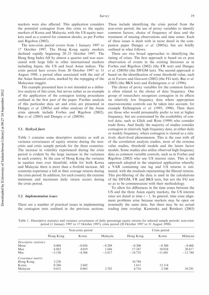
Table 1 contains some descriptive statistics as well asvariance–covariances of equity returns during the non-crisis and crisis sample periods for the three countries.The increase in volatility experienced during the crisisperiod is evident by the large increase in the variancesin each country. In the case of Hong Kong the variancein equities rises over threefold, while for both Koreaand Malaysia there is more than a fivefold increase. Allcountries experience a fall in their average returns duringthe crisis period. In addition, for each country the extrememinimum and maximum daily return occurs duringthe crisis period.

5.2. Implementation issues

There are a number of practical issues in implementingthe contagion tests outlined in the previous sections.

These include identifying the crisis period from thenon-crisis period, the use of proxy variables to identifycommon factors, choice of frequency of data and thetreatment of missing observations and time zones. Eachof these issues is dealt with in more detail in the com-panion paper Dungey et al. (2005a), but are brieflyoutlined in what follows.

There are two broad approaches to identifying thetiming of crises. The first approach is based on ex postobservation of events in the existing literature as inForbes and Rigobon (2002) (the FR test) and Dungeyet al. (2005b) (the DFGM test). The second approach isbased on the identification of some threshold value, suchas in Favero and Giavazzi (2002) (the FG test), Bae et al.(2003) (the BKS test) and Eichengreen et al. (1996).

The choice of proxy variables for the common factorsis often related to the choice of data frequency. Onegroup of researchers recognizes contagion in its effectson relatively low frequency data where appropriatemacroeconomic controls can be taken into account, forexample Eichengreen et al. (1995, 1996). Then thereare those who would presumably prefer to test at higherfrequency, but are constrained by the availability of con-trol data, such as Glick and Rose (1999) who considertrade flows. And finally the majority of studies considercontagion in relatively high frequency data, at either dailyor weekly frequency, where contagion is viewed as a rela-tively short-lived phenomenon. This is the case with allof the correlation analysis studies, most of the extremevalue studies, threshold models and the latent factormodels. Some studies also utilize observed high frequencydata as common variable controls, such as in Forbes andRigobon (2002) who use US interest rates. This is theapproach adopted in the empirical application wherebya VAR containing one lag and US returns is esti-mated, with the residuals representing the filtered returns.This pre-filtering of the data is used in the calculationsof the DFGM, FR and BKS tests, but not the FG testso as to be commensurate with their methodology.

To allow for differences in the time zones between theUS and the three Asian equity markets, the US interestrates are dated at time t� 1. In general, time zone align-ment problems arise because markets may be open onnominally the same date, but there may be no actualtrading time overlap. Kaminsky and Reinhart (2003)

Table 1. Descriptive statistics and variance–covariances of daily percentage equity returns for selected sample periods: non-crisisperiod (1 January 1997 to 17 October 1997), crisis period (20 October 1997 to 31 August 1998).

Non-crisis period Crisis period

Hong Kong Korea Malaysia Hong Kong Korea Malaysia

Descriptive statisticsMean 0.004 �0.056 �0.209 �0.300 �0.300 �0.468Max 6.883 4.019 1.666 17.247 10.024 20.817Min �5.150 �4.306 �5.817 �14.735 �11.601 �11.744

Covariance matrixHong Kong 2.238 10.794Korea 0.260 2.045 1.611 13.114Malaysia 0.631 0.063 2.782 4.716 3.348 10.291

Survey 19

Dow

nloa

ded

by [

Uni

vers

ity o

f Sa

skat

chew

an L

ibra

ry]

at 0

0:27

24

Sept

embe

r 20

12

find significant time zone effects in equity markets. Oneapproach to this problem is to control for differences intime zones by using moving averages of returns (Forbesand Rigobon 2002, Ellis and Lewis 2000). However,this may mask movements in asset prices and hence intro-duce biases into the tests of contagion. Bae et al. (2003)choose different lags depending on the time zone underinvestigation, which works because two distinct timezones are involved. Dungey et al. (2003a) suggest usingsimulation methods by treating time zone problemsas a missing observation issue.

Finally, missing observations cause problems in track-ing volatility across markets in a single period, and areusually dealt with by either replacing the missing observa-tion with the previous market observation or removingthat data point from the investigation. In practice,most researchers seem to use a strategy of excludingdays corresponding to missing observations, which isthe approach adopted below.

5.3. Contagion testing

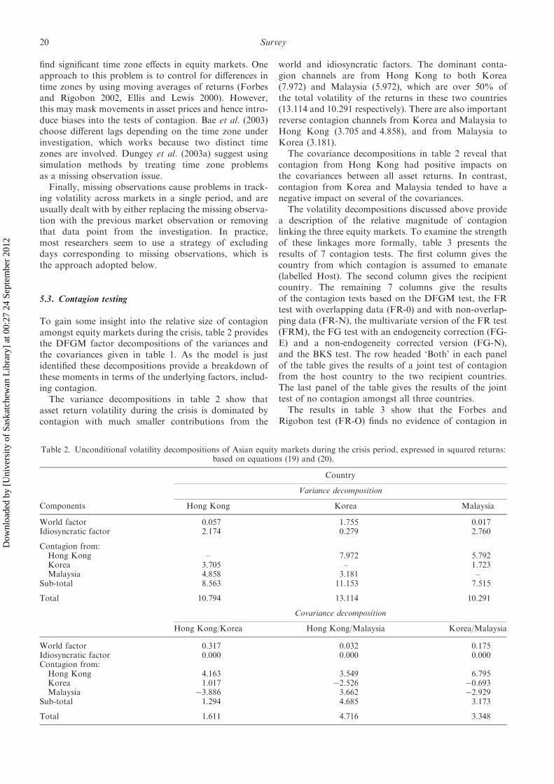
To gain some insight into the relative size of contagionamongst equity markets during the crisis, table 2 providesthe DFGM factor decompositions of the variances andthe covariances given in table 1. As the model is justidentified these decompositions provide a breakdown ofthese moments in terms of the underlying factors, includ-ing contagion.

The variance decompositions in table 2 show thatasset return volatility during the crisis is dominated bycontagion with much smaller contributions from the

world and idiosyncratic factors. The dominant conta-gion channels are from Hong Kong to both Koreað7:972Þ and Malaysia ð5:972Þ, which are over 50% ofthe total volatility of the returns in these two countriesð13:114 and 10.291 respectivelyÞ. There are also importantreverse contagion channels from Korea and Malaysia toHong Kong ð3:705 and 4:858Þ, and from Malaysia toKorea ð3:181Þ.

The covariance decompositions in table 2 reveal thatcontagion from Hong Kong had positive impacts onthe covariances between all asset returns. In contrast,contagion from Korea and Malaysia tended to have anegative impact on several of the covariances.

The volatility decompositions discussed above providea description of the relative magnitude of contagionlinking the three equity markets. To examine the strengthof these linkages more formally, table 3 presents theresults of 7 contagion tests. The first column gives thecountry from which contagion is assumed to emanate(labelled Host). The second column gives the recipientcountry. The remaining 7 columns give the resultsof the contagion tests based on the DFGM test, the FRtest with overlapping data (FR-0) and with non-overlap-ping data (FR-N), the multivariate version of the FR test(FRM), the FG test with an endogeneity correction (FG-E) and a non-endogeneity corrected version (FG-N),and the BKS test. The row headed ‘Both’ in each panelof the table gives the results of a joint test of contagionfrom the host country to the two recipient countries.The last panel of the table gives the results of the jointtest of no contagion amongst all three countries.

The results in table 3 show that the Forbes andRigobon test (FR-O) finds no evidence of contagion in

Table 2. Unconditional volatility decompositions of Asian equity markets during the crisis period, expressed in squared returns:based on equations (19) and (20).

Country

Variance decomposition

Components Hong Kong Korea Malaysia

World factor 0.057 1.755 0.017Idiosyncratic factor 2.174 0.279 2.760

Contagion from:Hong Kong – 7.972 5.792Korea 3.705 – 1.723Malaysia 4.858 3.181 –

Sub-total 8.563 11.153 7.515

Total 10.794 13.114 10.291

Covariance decomposition

Hong Kong/Korea Hong Kong/Malaysia Korea/Malaysia

World factor 0.317 0.032 0.175Idiosyncratic factor 0.000 0.000 0.000Contagion from:Hong Kong 4.163 3.549 6.795Korea 1.017 �2.526 �0.693Malaysia �3.886 3.662 �2.929

Sub-total 1.294 4.685 3.173

Total 1.611 4.716 3.348

20 Survey

Dow

nloa

ded

by [

Uni

vers

ity o

f Sa

skat

chew

an L

ibra

ry]

at 0

0:27

24

Sept

embe

r 20

12

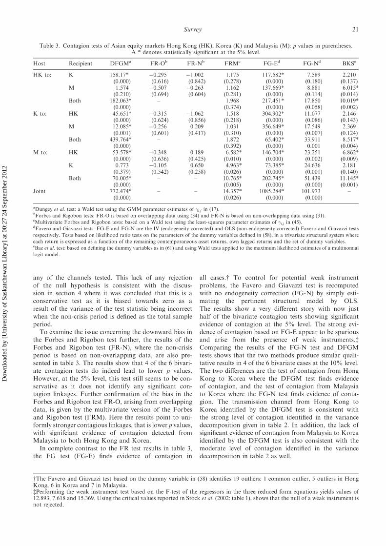
any of the channels tested. This lack of any rejectionof the null hypothesis is consistent with the discus-sion in section 4 where it was concluded that this is aconservative test as it is biased towards zero as aresult of the variance of the test statistic being incorrectwhen the non-crisis period is defined as the total sampleperiod.

To examine the issue concerning the downward bias inthe Forbes and Rigobon test further, the results of theForbes and Rigobon test (FR-N), where the non-crisisperiod is based on non-overlapping data, are also pre-sented in table 3. The results show that 4 of the 6 bivari-ate contagion tests do indeed lead to lower p values.However, at the 5% level, this test still seems to be con-servative as it does not identify any significant con-tagion linkages. Further confirmation of the bias in theForbes and Rigobon test FR-O, arising from overlappingdata, is given by the multivariate version of the Forbesand Rigobon test (FRM). Here the results point to uni-formly stronger contagious linkages, that is lower p values,with signifciant evidence of contagion detected fromMalaysia to both Hong Kong and Korea.

In complete contrast to the FR test results in table 3,the FG test (FG-E) finds evidence of contagion in

all cases.y To control for potential weak instrumentproblems, the Favero and Giavazzi test is recomputedwith no endogeneity correction (FG-N) by simply esti-mating the pertinent structural model by OLS.The results show a very different story with now justhalf of the bivariate contagion tests showing significantevidence of contagion at the 5% level. The strong evi-dence of contagion based on FG-E appear to be spuriousand arise from the presence of weak instruments.zComparing the results of the FG-N test and DFGMtests shows that the two methods produce similar quali-tative results in 4 of the 6 bivariate cases at the 10% level.The two differences are the test of contagion from HongKong to Korea where the DFGM test finds evidenceof contagion, and the test of contagion from Malaysiato Korea where the FG-N test finds evidence of conta-gion. The transmission channel from Hong Kong toKorea identified by the DFGM test is consistent withthe strong level of contagion identified in the variancedecomposition given in table 2. In addition, the lack ofsignificant evidence of contagion from Malaysia to Koreaidentified by the DFGM test is also consistent with themoderate level of contagion identified in the variancedecomposition in table 2 as well.

Table 3. Contagion tests of Asian equity markets Hong Kong (HK), Korea (K) and Malaysia (M): p values in parentheses.A * denotes statistically significant at the 5% level.

Host Recipient DFGMa FR-Ob FR-Nb FRMc FG-Ed FG-Nd BKSe

HK to: K 158.17* �0.295 �1.002 1.175 117.582* 7.589 2.210(0.000) (0.616) (0.842) (0.278) (0.000) (0.180) (0.137)

M 1.574 �0.507 �0.263 1.162 137.669* 8.881 6.015*(0.210) (0.694) (0.604) (0.281) (0.000) (0.114) (0.014)

Both 182.063* – 1.968 217.451* 17.850 10.019*(0.000) (0.374) (0.000) (0.058) (0.002)

K to: HK 45.651* �0.315 �1.062 1.518 304.902* 11.077 2.146(0.000) (0.624) (0.856) (0.218) (0.000) (0.086) (0.143)

M 12.085* �0.256 0.209 1.031 356.649* 17.549 2.369(0.001) (0.601) (0.417) (0.310) (0.000) (0.007) (0.124)

Both 439.764* – 1.872 65.402* 33.911 8.517*(0.000) (0.392) (0.000) 0.001 (0.004)

M to: HK 53.578* �0.348 0.189 6.582* 146.704* 23.251 6.862*(0.000) (0.636) (0.425) (0.010) (0.000) (0.002) (0.009)

K 0.773 �0.105 0.650 4.963* 73.385* 24.636 2.181(0.379) (0.542) (0.258) (0.026) (0.000) (0.001) (0.140)

Both 70.005* – – 10.765* 202.745* 51.439 11.145*(0.000) (0.005) (0.000) (0.000) (0.001)

Joint 772.474* – – 14.357* 1085.284* 101.973 –(0.000) (0.026) (0.000) (0.000)

aDungey et al. test: a Wald test using the GMM parameter estimates of �i;j in (17).bForbes and Rigobon tests: FR-O is based on overlapping data using (34) and FR-N is based on non-overlapping data using (31).cMultivariate Forbes and Rigobon tests: based on a Wald test using the least-squares parameter estimates of �i;j in (45).dFavero and Giavazzi tests: FG-E and FG-N are the IV (endogeneity corrected) and OLS (non-endogeneity corrected) Favero and Giavazzi tests

respectively. Tests based on likelihood ratio tests on the parameters of the dummy variables defined in (58), in a trivariate structural system where

each return is expressed as a function of the remaining contemporaneous asset returns, own lagged returns and the set of dummy variables.eBae et al. test: based on defining the dummy variables as in (61) and using Wald tests applied to the maximum likelihood estimates of a multinomial

logit model.

yThe Favero and Giavazzi test based on the dummy variable in (58) identifies 19 outliers: 1 common outlier, 5 outliers in HongKong, 6 in Korea and 7 in Malaysia.zPerforming the weak instrument test based on the F-test of the regressors in the three reduced form equations yields values of12.893, 7.618 and 15.369. Using the critical values reported in Stock et al. (2002: table 1), shows that the null of a weak instrument isnot rejected.

Survey 21

Dow

nloa

ded

by [

Uni

vers

ity o

f Sa

skat

chew

an L

ibra

ry]

at 0

0:27

24

Sept

embe

r 20

12

The last test results reported in table 3 are for the Baeet al. (BKS) test.y Comparing the bivariate DFGM andBKS results shows that the two testing procedures giveopposite results where Hong Kong and Korea are thehosts, but the same results where Malaysia is the host.Part of the explanation underlying these results couldbe the dating of the crisis period which is determineda priori in the case of the DFGM test, whereas for theBKS test is determined endogenously. An additional issuesurrounding the BKS test is that it discards informationin constructing the dummy dependent and independentvariables, which may in turn lead to a loss of efficienyin the parameter estimates.

In general, these results in table 3 provide evidenceof the difficulties in obtaining consistent information onthe existence of contagion from the different tests. Thisis not unique to this example, similar outcomes emergein other applied examples for the 1994 Mexican crisis andthe 2001 Argentine crisis provided in Dungey et al.(2005a). Some of these problems are shown by Dungeyet al. (2004) to be due to low power and poor size proper-ties of these various tests of contagion.

6. Conclusions and suggestions for future research

This paper has overviewed a number of important testsfor the presence and characteristics of contagion in finan-cial markets adopted in the current literature. Using aframework of a latent factor model similar to thatproposed in the finance literature, the different testingmethodologies are shown to be related. In essence, eachmethod is shown to be a test on a common parameterregarding the transmission of a shock from one countryor market to another.

An important result of this paper is that the main dis-tinguishing feature of alternative empirical models of con-tagion is the way in which the information is used toidentify contagion. Dungey et al. (2005b) and Forbesand Rigobon (2002) use the information on all of theshocks in the crisis period to test for contagion. Undercertain conditions these two models are the same. Faveroand Giavazzi (2002) utilize shift dummies at selected crisispoints to represent potentially contagious transmissions.Eichengreen et al. (1995, 1996) also use dummy variablesto identify contagion, however they transform both thedependent and independent indicators into binary vari-ables, which results in a further reduction of the informa-tion used in estimation. Bae et al. (2003) provide anextension of the Eichengreen et al. approach by allowingfor a polychotomous dependent variable, based on thenumber of co-exceedances in their crisis indicator.

Some of the properties and relationships of the variouscontagion tests were demonstrated in an empirical appli-cation of the Asian crisis of 1997–1998. A number ofempirical issues concerning missing observations, time

zones, dating of crises and data frequency were also dis-cussed. The results showed that the Forbes and Rigoboncontagion test was a conservative test as it failed to findevidence of contagion in any of the linkages tested. TheFavero and Giavazzi test was at the other extreme, find-ing evidence of contagion in all cases investigated. Muchof this evidence of linkages was found to be spurious,being the result of weak instruments. Correcting theFavero and Giavazzi test for weak instruments yieldedcontagion channels similar to the channels identified bythe DFGM test. The BKS test results tended to be incon-sistent with the results of these last two tests. In general,the empirical results of the tests highlighted the need forinvestigating the sampling properties of the various testswith an extensive Monte Carlo design that looks at issuessuch as the dating of crises, the modelling of dynamics,the information effects of filtering. Some of these issueshave been tackled in Dungey et al. (2004) who use anumber of Monte Carlo experiments to demonstratethe size and power properties of many of these tests.

Acknowledgments

This project was funded under ARC large grantA00001350. We are grateful for comments from theeditors, three anonymous referees, Dirk Baur, DavidCook, Roger Craine, Jon Danielsson, Amil Dasgupta,Barry Eichengreen, Charles Goodhart, Don Harding,Paul Masson, Hashem Pesaran, Andreas Pick, RobertoRigobon, Hyun Shin, Demosthenes Tambakis and parti-cipants at seminars and conferences where this workhas been presented. The paper was partly written whileMardi Dungey was a Visiting Fellow at CERF. The viewsexpressed in this paper are those of the authors anddo not necessarily coincide with those of the IMF orIMF policy.

References

Allen, F. and Gale, D., Financial contagion. J. Polit. Econ.,2000, 108, 1–33.

Bae, K.H., Karolyi, G.A. and Stulz, R.M., A new approachto measuring financial contagion. Rev. Financ. Stud., 2003,16(3), 717–763.

Baig, T. and Goldfajn, I., The Russian default and thecontagion to Brazil. IMF Working Paper WP/00/160,2000 (IMF).

Bayoumi, T., Fazio, G., Kumar, M. and MacDonald, R., Fatalattraction: a new measure of contagion. IMF Working PaperWP/03/80, 2003 (IMF).

Bekaert, G., Harvey, C.R. and Ng, A., Market integrationand contagion. J. Bus., 2005, 78(1), 39–69.

Bekaert, G. and Hodrick, R., Characteristing predictablecomponents in excess returns on equity and foreign exchangemarkets. J. Finance, 1992, 47, 467–509.

Boyer, B.H., Gibson, M.S. and Loretan, M., Pitfalls in testsfor changes in correlations. Working Paper 597R, 1999(Federal Reserve Board, International Finance Division).

yThe BKS test is based on 22 exceedances, 4 co-exceedances between Hong Kong and Korea, 5 co-exceedances between Hong Kongand Malaysia and 4 co-exceedances between Korea and Malaysia.

22 Survey

Dow

nloa

ded

by [

Uni

vers

ity o

f Sa

skat

chew

an L

ibra

ry]

at 0

0:27

24

Sept

embe

r 20

12

Butler, K.C. and Joaquin, D.C., Are the gains from interna-tional portfolio diversification exaggerated? The influenceof downside risk in bear markets? J. Int. Money Finance,2002, 21, 981–1011.

Calvo, S. and Mendoza, E., Rational contagion and theglobalization of securities markets. J. Int. Econ., 2000,51, 79–113.

Caporale, G.M., Cipollini, A. and Spagnolo, N., Testing forcontagion: a conditional correlation analysis. DiscussionPaper No. 01-2002, 2002 (Centre for Monetary andFinancial Economics, South Bank University).

Chernov, M.E., Gallant, R.A., Ghysels, E. and Tauchen, G.,Alternative models for stock price dynamics.J. Econometrics, 2003, 116, 225–257.

Chue, T.K., Time varying risk preferences and emergingmarket covariances. J. Int. Money Finance, 2002, 21,1053–1072.

Cizeau, P., Potters, M. and Bouchard, J., Correlationstructure of extreme stock returns. Quant. Finance, 2001,1(2), 217–222.

Corsetti, G., Pericoli, M. and Sbracia, M., Correlation analysisof financial contagion: what one should know before runninga test. Mimeo, 2001 (University of Rome III).

Corsetti, G., Pericoli, M. and Sbracia, M., ‘Some contagion,some interdependence’: more pitfalls in testing for contagion.Mimeo, 2003 (University of Rome III).

Diebold, F.X. and Nerlove, M., The dynamics of exchangerate volatility: a multivariate latent-factor ARCH model.J. Appl. Econometrics, 1989, 4, 1–22.

Dornbusch, R., Park, Y.C. and Claessens, S., Contagion:understanding how it spreads. World Bank Res. Obs., 2000,15(2), 177–97.

Dungey, M., Fry, R., Gonzalez-Hermisillo, B. and Martin, V.L.,The transmission of contagion in developed and developinginternational bond markets, in Risk Measurement andSystemic Risk, Proceedings of the Third Joint CentralBank Research Conference, edited by Committee on theGlobal Financial System, 2002, pp. 61–74.

Dungey, M., Fry, R.A., Gonzalez-Hermosillo, B. andMartin, V.L., Unanticipated shocks and systemic influences:the impact of contagion in global equity markets in 1998.IMF Working Paper WP/03/84, 2003a (IMF).

Dungey, M., Fry, R.A., Gonzalez-Hermosillo, B. andMartin, V.L., A Monte Carlo analysis of alternative testsof contagion. Mimeo, 2004 (Australian National University).

Dungey, M., Fry, R.A., Gonzalez-Hermosillo, B. and Martin,V.L., A comparison of alternative tests of contagion withapplications. In Identifying International FinancialContagion: Progress and Challenges, edited by M. Dungeyand D. Tambakis, 2005a (Oxford University Press: Oxford)(in the press).

Dungey, M., Fry, R.A., Gonzalez-Hermosillo, B. andMartin, V.L., International contagion effects from theRussian crisis and the LTCM near-collapse. J. Financ.Stability, 2005b (in the press).

Dungey, M., Fry, R.A., and Martin, V.L., Equity transmissionmechanisms from Asia to Australia: interdependence or con-tagion? Aust. J. Manage., 2003b, 28(2), 157–182.

Dungey, M. and Martin, V.L., Contagion across financial mar-kets: an empirical assessment. New York Stock ExchangeConference Paper, 2001.

Dungey, M. and Martin, V.L., A multifactor model of exchangerates with unanticipated shocks: measuring contagion in theeast Asian currency crisis. J. Emerging Mark. Finance, 2004,3(3), 305–330.

Dungey, M., Martin, V.L. and Pagan, A.R., A multivariatelatent factor decomposition of international bond yieldspreads. J. Appl. Econometrics, 2000, 15(6), 697–715.

Dungey, M. and Zhumabekova, D., Testing for contagionusing correlations: some words of caution. Pacific BasinWorking Paper PB01-09, 2001 (Federal Reserve Bank ofSan Francisco).

Durbin, J.M., Errors in variables. Rev. Int. Stat. Inst., 1954, 22,23–32.

Eichengreen, B., Rose, A.K. and Wyplosz, C., Exchange marketmayhem: the antecedents and aftermath of speculativeattacks. Econ. Policy, 1995, 21, 249–312.

Eichengreen, B., Rose, A.K. and Wyplosz, C., Contagiouscurrency crises. NBER Working Paper 5681, 1996 (NationalBureau of Economic Research).

Ellis, L., and Lewis, E., The response of financial marketsin Australia and New Zealand to news about the Asiancrisis, in BIS Conference on International Financial Marketsand the Implications for Monetary and Financial Stability,Vol. 8, 2000 (Bank for International Settlements (BIS)).

Engle R.F., Ito, T. and Lin, W., Meteor showers or heat waves?Heteroskedastic intra-daily volatility in the foreign exchangemarket. Econometrica, 1990, 58, 525–542.

Engle, R.F. and Kroner, K.F., Multivariate simultaneousgeneralized ARCH. Econometric Theory, 1995, 11(1),122–150.

Favero, C.A. and Giavazzi, F., Is the international propagationof financial shocks non-linear? Evidence from the ERM.J. Int. Econ., 2002, 57(1), 231–246.

Flood, R. and Marion, N., Perspectives on the recent currencycrisis literature. NBER Working Paper #6380, 1998 (NationalBureau of Economic Research).

Flood, R. and Rose, A.K., Equity integration in times of crisis.Mark. Discipline, 2005 (in the press).

Forbes, K. and Rigobon, R., No contagion, only interdepen-dence: measuring stock market co-movements. J. Finance,2002, 57(5), 2223–2261.

Glick, R. and Rose, A.K., Contagion and trade: why arecurrency crises regional? J. Int. Money Finance, 1999,18(4), 603–617.

Granger, C., Huang, B., and Yang, C., A bivariate causalitybetween stock prices and exchange rates: evidence from recentAsian flu. Q. Rev. Econ. Finance, 2000, 40, 337–354.

Grubel, H.G. and Fadner, R., The interdependence of inter-national equity markets. J. Finance, 1971, 26, 89–94.

Hartmann, P., Straetmans, S. and de Vries, C.G., Assetmarket linkages in crisis periods. Rev. Econ. Stat., 2004, 86,313–326.

Jeanne, O. and Masson, P., Currency crises, sunspots andMarkov-switching regimes. J. Int. Econ., 2000, 50(2),327–350.

Kaminsky, G.L. and Reinhart, C.M., On crises, contagion andconfusion. J. Int. Econ., 2000, 51(1), 145–168.

Kaminsky, G.L. and Reinhart, C.M., Financial markets in timesof stress. NBER Working Paper #8569, 2001 (NationalBureau of Economic Research).

Kaminsky, G.L. and Reinhart, C.M., The Center andthe Periphery: The Globalization of Financial Turmoil,NBER Working Paper 9479, 2003 (National Bureau ofEconomic Research).

Kaminsky, G.L. and Schmukler, S.L., What triggers marketjitters? A chronicle of the Asian crisis. J. Int. MoneyFinance, 1999, 18, 537–560.

Karolyi, A. and Stulz, R., Why do markets move together?An investigation of US–Japan stock return comovements.J. Finance, 1996, 51(3), 951–986.

Kendall, M. and Stuart, A., The Advanced Theory of Statistics,Vol. 2, 1973 (Charles Griffin and Co.: London).

Kendall, M. and Stuart, A., The Advanced Theory of Statistics,Vol. 1, 1969 (Charles Griffin and Co.: London).

King, M. and Wadhwani, S., Transmission of volatility betweenstock markets. Rev. Financ. Stud., 1990, 3(1), 5–33.

Kiyotaki, N. and Moore, J., Balance-sheet contagion. Am. Econ.Rev. Papers Proc., 2002, 92(2), 46–50.

Kodres, L.E. and Pritsker, M., A rational expectations model offinancial contagion. J. Finance, 2002, 57(2), 768–799.

Kyle, A. and Xiong, W., Contagion as a wealth effect.J. Finance, 2001, 56(4), 1401–1440.

Survey 23

Dow

nloa

ded

by [

Uni

vers

ity o

f Sa

skat

chew

an L

ibra

ry]

at 0

0:27

24

Sept

embe

r 20

12

Longin, F. and Solnik, B., Is the correlation in internationalequity returns constant: 1960–1990? J. Int. Money Finance,1995, 14(1), 3–26.

Loretan, M. and English, W., Evaluating ‘correlation break-downs’ during periods of market volatility. InternationalFinance Discussion Paper No. 658, 2000 (Board ofGovernors of the Federal Reserve System).

Mahieu, R. and Schotman, P., Neglected common factorsin exchange rate volatility. J. Empirical Finance, 1994, 1,279–311.

Malliaroupulos, D., A multivariate GARCH model of riskpremia in foreign exchange markets. Econ. Modelling, 1997,14, 61–79.

Masson, P., Contagion: macroeconomic models with multipleequilibria. J. Int. Money Finance, 1999a, 18, 587–602.

Masson, P., Contagion: monsoonal effects, spillovers, andjumps between multiple equilibria. In The Asian FinancialCrisis: Causes, Contagion and Consequences, edited byP.R. Agenor, M. Miller, D. Vines and A. Weber, 1999b(Cambridge University Press: Cambridge, Thailand).

Masson, P., Multiple equilibria, contagion and the emergingmarket crises. IMF Working Paper #99/164, 1999c (IMF).

Mody, A. and Taylor, M.P., Common vulnerabilities. Mimeo,2003 (University of Warwick).

Nelson, C.R. and Startz, R., The distribution of the instru-mental variables estimator and its t-ratio when the instrumentis a poor one. J. Bus., 1990, 63, S125–S140.

Pericoli, M. and Sbracia, M., A primer on financial contagion.J. Econ. Surveys, 2003, 17(4), 571–608.

Pesaran, H. and Pick, A., Econometric issues in the analysisof contagion. CESifo Working Paper 1176, 2003 (CESifo).

Rigobon, R., The curse of non-investment grade countries.J. Develop. Econ., 2002, 69, 423–449.

Rigobon, R., Identification through heteroskedasticity.Rev. Econ. Stat., 2003a, 85(4), 777–792.

Rigobon, R., On the measurement of the international prop-ogation of shocks: is the transmission stable? J. Int. Econ.,2003b, 61, 261–283.

Sharpe, W., Capital asset prices: a theory of market equilibriumunder conditions of risk. J. Finance, 1964, 19, 425–442.

Solnik, B.H., The international pricing of risk: an empiricalinvestigation of the world capital market structure.J. Finance, 1974, 29(2), 365–378.

Stock, J.H., Wright, J.H. and Yogo, M., A survey of weakinstruments and weak identification in generalized methodof moments. J. Bus. Econ. Stat., 2002, 20(4), 518–529.

Toyoda, T. and Ohtani, K., Testing equality between setsof coefficients after a preliminary test for equality of distur-bance variances in two linear regressions. J. Econometrics,1986, 31, 67–80.

Wald, A., The fitting of straight lines if both variables aresubject to error. Ann. Math. Stat., 1940, 11, 284–300.

Van Rijckeghem, C.V. and Weder, B., Sources of contagion: isit finance or trade? J. Int. Econ., 2001, 54, 293–300.

24 Survey

Dow

nloa

ded

by [

Uni

vers

ity o

f Sa

skat

chew

an L

ibra

ry]

at 0

0:27

24

Sept

embe

r 20

12