Empirical Essays in Health and Education Economics
119
Empirical Essays in Health and Education Economics Inaugural-Dissertation zur Erlangung des Grades Doctor oeconomiae publicae (Dr. oec. publ.) an der Ludwig-Maximilians-Universität München 2010 vorgelegt von Amelie Catherine Wuppermann Referent: Prof. Dr. Joachim Winter Korreferent: Prof. Dr. Florian Heiss Promotionsabschlussberatung: 1. Juni 2011
Transcript of Empirical Essays in Health and Education Economics

Empirical Essaysin
Health and Education Economics
Inaugural-Dissertationzur Erlangung des Grades
Doctor oeconomiae publicae (Dr. oec. publ.)an der Ludwig-Maximilians-Universität München
2010
vorgelegt vonAmelie Catherine Wuppermann
Referent: Prof. Dr. Joachim WinterKorreferent: Prof. Dr. Florian HeissPromotionsabschlussberatung: 1. Juni 2011

Acknowledgements
First and foremost, I would like to thank my supervisor, Joachim Winter. I am gratefulfor his critical questions, constructive comments and general support that have guidedme while writing this dissertation and beyond.
I would further like to thank my co-supervisor, Florian Heiss, for his guidance andcontinuous encouragement during the past years. Thanks also go to Ludger Wößmannfor advice on the fourth chapter of this dissertation and for agreeing to serve on mycommittee.
In addition, I am indebted to many people for their help with writing this disserta-tion. In particular, I would like to thank my coauthors, Helmut Farbmacher and GuidoSchwerdt, for the collaboration that has been and continues to be a source of inspi-ration and motivation. I would further like to thank Luc Bissonnette, Nicolas Sauter,Beatrice Scheubel and Hannes Schwandt for valuable suggestions and comments andPeter Ihle and Ingrid Schubert for data support.
I would like to thank Klaus Schmidt for convincing me to spend an academic year atthe University of Wisconsin-Madison and my professors and fellow-students at the eco-nomics department in Madison for the challenging and inspiring academic experience.I would also like to thank Dana Goldman and the Bing Center for Health Economicsfor giving me the opportunity to write part of this dissertation at RAND. Withoutmy stays in Madison and at the RAND Corporation in Santa Monica this dissertationwould not have been the same.
Finally, I gratefully acknowledge financial support from the Deutsche Forschungs-gemeinschaft through GRK 801 and from the German Academic Exchange Service.

Contents
Preface 1
1 Do I know more than my body can tell? 81.1 Introduction . . . . . . . . . . . . . . . . . . . . . . . . . . . . . . . . . 81.2 Empirical Literature on Adverse Selection . . . . . . . . . . . . . . . . 111.3 Data . . . . . . . . . . . . . . . . . . . . . . . . . . . . . . . . . . . . . 141.4 Estimation Strategy . . . . . . . . . . . . . . . . . . . . . . . . . . . . 181.5 Results . . . . . . . . . . . . . . . . . . . . . . . . . . . . . . . . . . . . 211.6 Robustness Analyses . . . . . . . . . . . . . . . . . . . . . . . . . . . . 271.7 Conclusion . . . . . . . . . . . . . . . . . . . . . . . . . . . . . . . . . . 33Appendix: Inverse Probability Weighting . . . . . . . . . . . . . . . . . . . . 36
2 Do they know what’s at risk? 382.1 Introduction . . . . . . . . . . . . . . . . . . . . . . . . . . . . . . . . . 382.2 Related Literature . . . . . . . . . . . . . . . . . . . . . . . . . . . . . 402.3 Data . . . . . . . . . . . . . . . . . . . . . . . . . . . . . . . . . . . . . 412.4 Estimation Methods . . . . . . . . . . . . . . . . . . . . . . . . . . . . 44
2.4.1 Calculation of Objective Risk . . . . . . . . . . . . . . . . . . . 442.4.2 Comparison Subjective and Objective Risk . . . . . . . . . . . . 47
2.5 Results . . . . . . . . . . . . . . . . . . . . . . . . . . . . . . . . . . . . 472.6 Robustness Analyses . . . . . . . . . . . . . . . . . . . . . . . . . . . . 512.7 Conclusion . . . . . . . . . . . . . . . . . . . . . . . . . . . . . . . . . . 54Appendix . . . . . . . . . . . . . . . . . . . . . . . . . . . . . . . . . . . . . 56
3 Heterogeneous Effects of Copayments 583.1 Introduction . . . . . . . . . . . . . . . . . . . . . . . . . . . . . . . . . 583.2 Econometric Framework . . . . . . . . . . . . . . . . . . . . . . . . . . 613.3 Data . . . . . . . . . . . . . . . . . . . . . . . . . . . . . . . . . . . . . 623.4 Results . . . . . . . . . . . . . . . . . . . . . . . . . . . . . . . . . . . . 64

Contents iii
3.4.1 Model Selection . . . . . . . . . . . . . . . . . . . . . . . . . . . 643.4.2 Average Effects and one-way Heterogeneities . . . . . . . . . . . 653.4.3 Simultaneous Evaluation of Heterogeneities . . . . . . . . . . . . 67
3.5 Conclusion . . . . . . . . . . . . . . . . . . . . . . . . . . . . . . . . . . 71Appendix: Marginal Effects . . . . . . . . . . . . . . . . . . . . . . . . . . . 73
4 Is traditional teaching really all that bad? 754.1 Introduction . . . . . . . . . . . . . . . . . . . . . . . . . . . . . . . . . 754.2 Literature on Teaching Practices . . . . . . . . . . . . . . . . . . . . . . 774.3 Data . . . . . . . . . . . . . . . . . . . . . . . . . . . . . . . . . . . . . 804.4 Estimation Strategy . . . . . . . . . . . . . . . . . . . . . . . . . . . . 854.5 Results . . . . . . . . . . . . . . . . . . . . . . . . . . . . . . . . . . . . 884.6 Robustness Checks . . . . . . . . . . . . . . . . . . . . . . . . . . . . . 944.7 Conclusion . . . . . . . . . . . . . . . . . . . . . . . . . . . . . . . . . . 98Appendix: Selection on Unobservables . . . . . . . . . . . . . . . . . . . . . 100
Bibliography 104

List of Tables
1.1 Descriptives – ELSA Wave 0 . . . . . . . . . . . . . . . . . . . . . . . . 131.2 Health Measures – ELSA Wave 0 . . . . . . . . . . . . . . . . . . . . . 151.3 Prevalence of Different Longstanding Illnesses – Wave 0 . . . . . . . . . 161.4 Information Used in Underwriting in US and UK Insurance Markets . . 201.5 Private Information on Mortality Risk – Women . . . . . . . . . . . . . 221.6 Private Information on Mortality Risk – Men . . . . . . . . . . . . . . 231.7 Private Information on Health Risk – Women . . . . . . . . . . . . . . 241.8 Private Information on Health Risk – Men . . . . . . . . . . . . . . . . 251.9 Robustness – Event by 2002 . . . . . . . . . . . . . . . . . . . . . . . . 281.10 Robustness – Subjective Life Expectancy . . . . . . . . . . . . . . . . . 291.11 Selection Mechanisms – Bivariate Probit . . . . . . . . . . . . . . . . . 37
2.1 Descriptive Statistics . . . . . . . . . . . . . . . . . . . . . . . . . . . . 432.2 Subjective and Objective Risk . . . . . . . . . . . . . . . . . . . . . . . 452.3 Duration Model for Disease Onsets in HRS . . . . . . . . . . . . . . . . 482.4 Differences Subjective and Objective Risk . . . . . . . . . . . . . . . . 502.5 Robustness Analyses I . . . . . . . . . . . . . . . . . . . . . . . . . . . 522.6 Robustness Analyses II . . . . . . . . . . . . . . . . . . . . . . . . . . . 532.7 Results for Smokers . . . . . . . . . . . . . . . . . . . . . . . . . . . . . 57
3.1 Descriptive Statistics . . . . . . . . . . . . . . . . . . . . . . . . . . . . 633.2 Model Selection . . . . . . . . . . . . . . . . . . . . . . . . . . . . . . . 653.3 Marginal Effects after Probit, FMM Probit and Bivariate Probit . . . . 663.4 FMM Bivariate Probit – Coefficients and Marginal Effects . . . . . . . 673.5 FMM Bivariate Probit – Marginal Effects on Joint Probabilities . . . . 69
4.1 Descriptive Statistics – Teacher variables . . . . . . . . . . . . . . . . . 824.2 Student, School and Class Variables by Intensity of Lecture Style Teaching 834.3 Teacher Variables by Intensity of Lecture Style Teaching . . . . . . . . 84

Contents v
4.4 Estimation Results OLS . . . . . . . . . . . . . . . . . . . . . . . . . . 894.5 Estimation Results First Difference . . . . . . . . . . . . . . . . . . . . 914.6 Robustness Checks I . . . . . . . . . . . . . . . . . . . . . . . . . . . . 954.7 Robustness Checks II: Absolute Time Specification . . . . . . . . . . . 974.8 Descriptive Statistics – Class Characteristics . . . . . . . . . . . . . . . 1024.9 Descriptive Statistics – Class Characteristics (cont.) . . . . . . . . . . . 103

List of Figures
1.1 SRH and Future Health Events - Men . . . . . . . . . . . . . . . . . . . 181.2 SRH and Future Health Events - Women . . . . . . . . . . . . . . . . . 181.3 Predicted Probability Death - Men . . . . . . . . . . . . . . . . . . . . 311.4 Predicted Probability Death - Women . . . . . . . . . . . . . . . . . . . 321.5 Predicted Probability Major Condition - Men . . . . . . . . . . . . . . 321.6 Predicted Probability Major Condition - Women . . . . . . . . . . . . . 33
3.1 Development of GP and Specialist Visits Over Time . . . . . . . . . . . 633.2 Predicted Probabilities in 2002 . . . . . . . . . . . . . . . . . . . . . . . 70

Preface
Health and education are two fields of economic research that are of relevance tothe political agenda in most developed countries. Governments play a major role inorganizing and financing health care and the education system. Market imperfectionsin both areas are put forward as rationale for government intervention (Poterba, 1996).
Imperfections in the health care market result mostly from informational asymme-tries. As future health care needs are to a large extent uncertain, a high proportion ofindividuals demand insurance. Asymmetric distributions of information between theinsurer and the user of health care, however, complicate the organization of healthinsurance. In particular, adverse selection and moral hazard may occur.
When the individuals who buy insurance are heterogeneous in terms of the insuredrisk and when they have more information on their risk than the insurer, adverseselection may result in market failure. Given a choice between different insuranceproducts, high risk individuals who know about their risk tend to choose generouscoverage. Correspondingly, individuals who know that their risk is lower tend to selectout of the respective insurance plans. Lower risk individuals are thus not able to obtaincomprehensive insurance coverage at a price corresponding to their risk (Cutler andZeckhauser, 2000, p. 606ff).
Moral hazard, on the other hand, induces individuals to demand more care thanthey would if they were not insured. Once individuals are insured, they do not haveto bear the full costs of medical treatments. If the insurer cannot observe the individ-uals’ actions or has limited means of judging whether a certain treatment is medicallyindicated, individuals might demand more – or more expensive – care than necessary.Copayments and other restrictions in the scope of insurance coverage are instrumentsto counteract this problem (Cutler and Zeckhauser, 2000, p. 576ff).
In the education system, market imperfections are mostly linked to externalities(Poterba, 1996). Not only the individual schooled but also the overall economy mightprofit from the individual’s education. Education might, for example, help to adopt newtechnologies of production and foster economic growth. When individuals choose theirlevel of education solely based on their individual costs and benefits, and do not take
Preface 2
into account the benefits that accrue for society as a whole, they may choose a lowerthan socially optimal level of education. It is thus frequently seen as a governmentresponsibility to subsidize the education system in order to induce socially optimallevels of education (Hanushek, 2002, p. 2064f.).
Health and education are on the political agenda today for different reasons. Healthcare costs have risen over the last decades. As a lot of the spending is public expen-diture, reforms of the health care system are needed to reduce costs and to complywith fiscal restrictions. Improving the education system is seen as a key to ensuringinternational competitiveness. While the question is not finally settled, the evidence isaccruing that higher levels of education foster economic growth (Hanushek and Woess-mann, 2009).
In order to provide guidance to respective reform efforts, empirical research bringstogether theoretical concepts, statistical methods and data. This dissertation con-tributes four empirical studies on questions related to health and education. Eachof the studies constitutes a self-contained chapter. The first three chapters focus onthe individual assessments of health risks and the organization of health care markets.Chapter 4 examines the impact of teaching methods on student achievement.
The analysis in chapter 1 is motivated by a puzzle in the literature on adverse se-lection. There is differential evidence of adverse selection in markets that are relatedto similar risks. In particular, empirical studies on life insurance markets find littleevidence of adverse selection but there is evidence of adverse selection in annuity mar-kets. Similarly, for some health insurance markets there is evidence of adverse selection,while others do not seem to be adversely selected. Cohen and Siegelman (2010) suggestthat different degrees of private information in the different markets result in differentscopes for adverse selection and might thus reconcile the mixed findings. Chapter 1provides an empirical evaluation of this explanation.
As similar risks are insured in the different markets, individual information on therisks is likely the same. Differences in private information could result from differencesin what the insurers know about the risks. The latter difference in turn can stem fromdifferences in information that the insurers collect and use for insurance underwriting,i.e. for risk assessment and calculation of premia.
A challenge of this analysis is thus to find a data set that includes informationon individuals’ and insurers’ risk assessments for potential buyers of insurance. As inmany circumstances everyone can potentially buy insurance, the analysis requires asample of the general population. Within general population surveys, however, typi-cally only a limited set of information on individual health risk factors are available.

Preface 3
The data set used in chapter 1 is an exception. It comes from the English LongitudinalStudy of Ageing (ELSA). ELSA collects a large set of variables that are typically alsocollected in the application process in some insurance markets. In particular, ELSAis one of the rare data sets that includes objectively measured health information col-lected by a nurse. As applicants in health-related insurance markets, such as privatehealth insurance and life insurance, typically have to disclose information from medi-cal examinations, ELSA is better suited to mimic the insurers’ information than othersurveys of the general population.
ELSA also comprises variables that can proxy for the potential buyers’ informationon their risk. The main analysis in chapter 1 uses individuals’ assessment of theirgeneral health as measure for the individual information. The measure is derived froma question in which individuals are asked to rate their general health on a 5-point scalefrom very good to very bad. The advantage that this measure has for the purpose ofmy study is that it is subjective. It cannot be verified by a third party. Informationthat is only contained in this self-rated health measure therefore necessarily remainsprivate.
Furthermore, ELSA is a panel study and thus tracks individuals over time. Thisallows to observe whether individuals actually experience the insured events in thefuture. In order to detect private information the statistical analysis conducted inchapter 1 combines the information on the occurrence of the insured event in thefuture, the proxy for the potential buyer’s information on the risk and the applicationinformation that insurers use for risk assessment. It is interpreted as evidence forprivate information if the proxy for the potential buyer’s information helps to predictthe future occurrence of the risks when the insurer’s information is controlled for.
The analysis shows that depending on the information that is used by the insurer toassess the potential buyers’ risk there are varying degrees of private information. Theresults can help to reconcile the mixed evidence on adverse selection in life insuranceand annuity markets and in different health insurance markets. Furthermore, theresults indicate that adverse selection may be overcome by accurate risk assessmentsby the insurers in the different insurance markets.
In contrast to chapter 1, the analysis in chapter 2 takes a direct approach to mea-suring individual risk perception by asking individuals how they rate their chances ofdeveloping different diseases in the future. Following the insights on measuring expec-tations summarized by Manski (2004), Joachim Winter and I implemented a survey onhealth expectations in the American Life Panel (ALP), an Internet panel administeredby RAND. We elicit the subjective health expectations as numerical probabilities. This

Preface 4
has an advantage over qualitative questions as it allows to gauge the accuracy of theindividual information by directly comparing it to objective probabilities.
The analysis presented in chapter 2 uses the subjective probabilities to shed light onthe question whether individuals who are overweight or obese are misinformed abouttheir health risks. The accuracy of risk perception among smokers has been analyzedbased on similar subjective probabilities by Schoenbaum (1997) and Khwaja et al.(2009). For individuals with excess weight a comparable study is not available so far.
Similar to smoking, obesity is responsible for a large share of health care costs(Cawley and Meyerhoefer, 2010). Furthermore, being obese is at least partly influencedby individual behavior. Behavioral changes could help to decrease an individual’s bodyweight. However, changes in behavior require an effort from the individual. Froma rational choice perspective, rational individuals would only engage in behavioralchanges if the benefits of doing so exceed the costs. If individuals who are overweightor obese underestimate their health risks, this implies that they underestimate thebenefits of behavioral changes.
While smokers are generally not found to underestimate their health risks, the re-sults for the overweight and obese presented in chapter 2 indicate that obese individualsunderestimate the risks of certain diseases. These results indicate that there is roomfor health education programs targeted at the obese population. More drastic cam-paigns on the risks of obesity similar to the campaigns on the risks of smoking mightbe needed in order to make individuals aware of their risks.
The third chapter is based on joint work with Helmut Farbmacher. Its focus lieson evaluating the effects of a recent reform in the German statutory health insurancesystem that increased copayments for doctor visits and prescription drugs in an effortto counteract moral hazard and thereby achieve cost containment. Augurzky et al.(2006), Schreyögg and Grabka (2010), Farbmacher (2010) and Rückert et al. (2008)have analyzed how the reform affected health care use among the statutorily insuredin Germany. The studies present inconclusive results on whether the reform changedindividual behavior.
The analysis presented in the third chapter contributes to this literature by usinga new data set. While the earlier studies rely on survey data, the data analyzed inchapter 3 is insurance claims data. It thus allows to reliably observe health care use.More importantly, however, the analysis goes beyond studying the average effect ofthe reform. It focuses on the question whether different groups of individuals reactdifferently to the reform. Bago d’Uva (2006) and Winkelmann (2006) find that thehealth care demand among individuals with high use of health care is less sensitive to
Preface 5
changes in prices than the demand among individuals with low use. We expand onthese two studies by changing the focus from demand for health care in general, to thedemand for different types of health care, namely visiting two different types of doctors– general practitioners (GPs) and specialists.
In order to conduct this analysis we develop a finite mixture bivariate probit model.On the one hand, this model allows for unobserved heterogeneity in terms of differentlatent classes of individuals. In particular, we assume that there are two groups ofindividuals that may differ in any observed and unobserved aspect. However, we donot observe which individual belongs to which group. After the estimation of themodel we can characterize the different groups in terms of their health care use. Onthe other hand, the bivariate probit component of the model allows to estimate howthe probability to visit different types of doctors is affected within each of the twolatent groups.
Our results indicate that the reform had an effect on individual behavior. Onaverage individuals are 3 percentage points less likely to visit any type of doctor atleast once within a year after the reform. In the application of the finite mixturebivariate probit model, we find that the two latent groups can be characterized asbeing likely to see a doctor and as being less-likely to see a doctor before the reform.The estimated probability of belonging to the likely users is 74%, indicating that this isthe majority of the population. Similar to Bago d’Uva (2006) and Winkelmann (2006)we find that the demand for health care is relatively more elastic among individualswho are less-likely to see a doctor before the reform.
Furthermore, distinguishing between the two types of doctor visits, we find thatthe patterns of use change differently in the different groups. While the reform inducesthe less-likely users to reduce their probability of visiting both types of doctors, thelikely users still visit GPs with the same probability after the reform. However, theyvisit a specialist with a smaller probability.
This result has an important implication for designing health care systems. Thecopayments do not force individuals to stop visiting specialists. A large part of thepopulation, however, visits a specialist with a smaller probability and instead focuseson GP visits as consequence of the reform. The GPs’ function in the health caresystem was therefore strengthened by the reform. Even though the reform did notimplement gatekeepers directly, meaning that individuals still have a choice betweengeneral practice and specialist care, it might have implemented effective incentives thatinduce a large fraction of the population to use GPs as if they were gatekeepers. Asit has been suggested that gatekeeping leads to lower health care costs (Scott, 2000),

Preface 6
the particular reform in the German health insurance might guide a way to introducegatekeeping without force.
The final chapter draws on joint work with Guido Schwerdt. It shifts the focusfrom health care reform to improving the education system. It attempts to answerthe question whether traditional teaching methods are related to worse educationaloutcomes than more modern approaches.
We use a data set for 8th grade students in the US from the Trends in Interna-tional Mathematics and Science Study (TIMSS) in 2003. This data set has two majoradvantages for our analysis and one disadvantage. The first advantage is that the dataallows to match students to teachers and we thus know which student was taught bywhich teachers. The second advantage is the panel dimension, namely that we observeeach student in two subjects. We observe how a student performed on the TIMSS testsin math and in science and which methods the teacher used in teaching the specificsubject. Taking differences between math and science for each student we employ afirst-difference method that allows us to control for any unobserved student traits thatare constant between the two subjects.
The disadvantage of the data set is that there is no random variation in teachingmethods. Teachers instead choose freely which methods they employ in teaching. Eventhough we can control for unobserved student characteristics, such as innate abilityor motivation, we are not able to identify causal effects of teaching methods. Forexample, there might be some unobserved teacher characteristic that induces teachersto choose a specific teaching method. If this teacher characteristic also makes a teachera good teacher, the estimated effect of the teaching method will be confounded with theeffect of the teacher characteristic. We evaluate how important this selection based onunobservable teacher characteristics is by borrowing a method pioneered in Altonji et al.(2005). This method essentially allows to estimate how large selection on unobservablecharacteristics would have to be compared to selection on observable characteristics inorder to explain an entire estimated effect.
The specific focus of our paper lies on comparing teaching using lecture style pre-sentation with teaching based on in-class problem solving. Our results indicate thatspending more time in class on lecture style teaching is significantly positively relatedto student performance, when controlling for subject-constant student traits. However,the application of the method pioneered by Altonji et al. indicates that selection onunobservable teacher traits could explain the entire estimated effect. We therefore re-frain from interpreting the estimated effect as causal and do not draw conclusions thatcall for more lecture style teaching. Nevertheless, based on our results it is implausible

Preface 7
that there is a negative effect of lecture style teaching. As our method helps to controlfor all other confounding factors, a true negative effect would only be consistent withfinding a positive correlation between lecture style teaching and student achievementif good teachers choose to teach with the bad teaching method. This, however, seemsto be rather implausible.

Chapter 1
Do I know more than my body cantell? An Empirical Analysis of PrivateInformation in Health-RelatedInsurance Markets
1.1 Introduction
Information asymmetries about risk types in competitive insurance markets are knownto induce inefficient outcomes due to adverse selection. In particular, the seminal modelby Rothschild and Stiglitz (1976) and various extensions robustly predict that higherrisk individuals buy more insurance coverage than lower risk individuals (Chiapporiet al., 2006). The empirical evidence on this matter, however, varies for differentinsurance markets (Cohen and Siegelman, 2010).
Several explanations have been put forward to reconcile theoretical and empiricalfindings. Multiple dimensions of asymmetric information, for example private infor-mation on risk preferences in addition to private information on risk type, can explainthe absence of adverse selection in some insurance markets (De Meza and Webb, 2001;Cutler et al., 2008a). Cohen and Siegelman (2010) suggest the absence of useful pri-vate information and thus the absence of scope for adverse selection in some but notin other insurance markets as an additional explanation for the mixed findings.
This chapter evaluates empirically whether different degrees of private informationexist in health-related insurance markets, in particular in the markets for life insurance,annuities, and health insurance. It attempts to reconcile the mixed findings that havebeen presented in the literature on adverse selection in the different insurance markets.

Do I know more than my body can tell? 9
While life insurance markets and private individual health insurance markets do notshow evidence of adverse selection, annuity markets and group health insurance marketsappear to be adversely selected.
Useful private information on the risk that is to be insured exists if a potentialbuyer of an insurance product has more information on the risk than the insurer. Eventhough the markets for life insurance and annuities, and different health insurance mar-kets insure similar risks and individuals thus likely have similar information a priori,differences in private information between these markets could exist, because insur-ance companies in the different markets collect and use different types of informationfor insurance underwriting, i.e. for risk classification and the calculation of premia.The variation in information used is at least partly due to legal restrictions. US fed-eral law, for example, prohibits employers from charging premia for health insurancebased on health-related information (GAO, 2003). Similarly, several US states haveintroduced community rating in combination with guaranteed issue laws for individualhealth insurance, entitling individuals to buy insurance coverage at a price dependingexclusively on abstract criteria such as sex, age or geographic region (Lo Sasso andLurie, 2009). In other private health insurance markets on the contrary health-relatedinformation is used in underwriting.1
Using data from the English Longitudinal Study of Ageing (ELSA), I analyze thescope for private information on the insured risks in life insurance markets, annuitymarkets, and health insurance markets by exploiting the different information used inunderwriting in the different insurance markets. As ELSA is a panel study, it allowsto track individuals over time. I can therefore observe whether events happen to theindividuals in the future that would result in insurance claims if the individuals wereinsured. I call this the information on the future ‘realization of risk’. In the mainanalysis, I interpret it as evidence for private information if a measure of individual’sself-rated health (SRH) helps to predict the future realization of risk when all infor-mation that the insurer uses in underwriting is controlled for.
SRH is thus employed as a proxy for individual information on the insured risks.It was chosen for two reasons: First, it significantly predicts future health events, likedeath and the onset of specific health conditions.2 As individuals with worse SRH are
1In addition to legal restrictions, political economy concerns (Finkelstein and Poterba, 2006), speci-ficities of the market structure (Kesternich and Schumacher, 2009), or different demand for underwrit-ing in the different markets (Browne and Kamiya, 2009) could explain the use of different informationin underwriting.
2For overviews on studies analyzing the relationship between SRH and subsequent death see Idlerand Benyamini (1997), and DeSalvo et al. (2006). Banks et al. (2007) provide evidence for relationshipsbetween SRH and future diagnoses of diseases.

Do I know more than my body can tell? 10
more likely to die sooner and more likely to get certain diseases in the future, SRHpresumably captures useful information on the insured risks in the insurance marketsthat I focus on. Second, SRH is a non-verifiable measure in the sense that insurancecompanies have no means to verify whether an individual’s statement of SRH is true.This is in contrast to other self-reported measures like an individual’s co-morbiditiesor family health history which can be verified by going back to health records. Itsnon-verifiability makes SRH particularly valuable for analyzing the existence of privateinformation. Information about health-related risks that is only contained in SRHnecessarily remains private.
The ELSA data set contains a broad range of health measures that correspond tothe information collected and used by insurance companies in underwriting. ELSA isone of the few longitudinal data sets that provides health data which are objectivelymeasured and reported by a nurse: Results of a blood sample analysis, blood pressuremeasurement, objectively measured body mass index (BMI), and waist-hip-ratio areavailable. As the objectively measured data are already available in an early wave ofthe survey, up to 10 years of follow-up can be used for the analysis.3
The realization of the risk that is insured in life insurance and annuity marketsis measured by an indicator for whether an individual dies within 10 years after thebaseline interview. The realization of the insured risk in health insurance markets iscaptured by a variable that indicates whether an individual is newly diagnosed or hasa recurrence of heart disease, cancer or stroke within 8 years after the initial interview.These conditions belong to the most costly conditions at the per capita level (Drusset al., 2002) and thus seem to be reasonable proxies for the risk insured in healthinsurance markets, namely high medical expenses.
My results indicate that SRH contains information on dying within or surviving thenext 10 years and on being diagnosed with one of the costly major health conditions inthe next 8 years, when only a limited number of additional control variables is includedin the analysis. With the inclusion of medical information and in particular with theinclusion of the objectively measured health data, however, the explanatory power ofSRH is significantly reduced. The explanatory power of SRH for the onset of the costlyhealth conditions even vanishes completely. These results are robust to using differentproxies for the individual information on risks.
The results in combination with different use of information for underwriting in dif-ferent insurance markets can help to explain the mixed evidence of adverse selection in
3The US Health and Retirement Study has recently also started to collect objectively measuredhealth information. Up to now at most 1 wave, i.e. 2 years, of follow-up is available, however.

Do I know more than my body can tell? 11
life insurance and annuity markets, and in different health insurance markets. While inlife insurance markets stringent underwriting is performed and no evidence is found foradverse selection, in annuity markets only limited information is used for underwritingand evidence for adverse selection is found. Similarly, in individual health insurancewith stringent underwriting no evidence is found for adverse selection, while in grouphealth insurance there is evidence for adverse selection and no individual underwritingis performed.
An implication of the results is that the scope for adverse selection in group healthinsurance markets and annuity markets could be reduced by employing more stringentunderwriting. Whether more stringent underwriting would increase welfare, however,cannot be determined based on my analysis. While stringent underwriting might miti-gate the effects of adverse selection, it might have consequences not taken into accountin my analysis. The overall welfare effect of stringent underwriting depends on the ex-act institutional setting. Health insurance, for example, is often bought in short-termcontracts, that is individuals have to buy coverage repeatedly over time. If every timewhen individuals buy coverage stringent underwriting is employed, individuals will facethe risk of ‘becoming a higher risk’ and thus having to pay higher prices for insurancein the future. Without an insurance for this additional risk stringent underwritingcould reduce welfare.
The chapter is structured as follows: Section 2 gives an overview on the empiricalevidence of adverse selection in health-related insurance markets, Section 3 introducesthe data used for the analysis. Section 4 outlines the estimation strategy, results areshown in Section 5, Section 6 reports the results of several robustness analyses, andthe last section concludes.
1.2 Empirical Literature on Adverse Selection
The empirical literature has analyzed whether adverse selection is present in manydifferent insurance markets, such as the markets for automobile insurance, crop insur-ance, long term care, reverse mortgages, life insurance, annuities, and health insurance.Cohen and Siegelman (2010) provide a recent overview on the empirical findings. Inthis section, I focus on the literature concerning the last three markets.
The empirical evidence of adverse selection varies between life insurance and an-nuity markets. While in markets for annuities evidence for adverse selection is found(Finkelstein and Poterba, 2002, 2004, 2006; McCarthy and Mitchell, 2010; Einav et al.,2010b), there is only very little evidence for adverse selection in life insurance markets.

Do I know more than my body can tell? 12
He (2009) finds evidence that individuals in the Health and Retirement Study (HRS)who newly buy life insurance die earlier than individuals who do not buy life insurancewhen controlling for variables that insurance companies use for risk classification andcalculation of premia. However, as there is no objectively measured health informationin the HRS waves that He uses in her analysis, her study might not sufficiently controlfor risk classification undertaken by the insurers. Furthermore, Cawley and Philipson(1999), Hendel and Lizzeri (2003) and McCarthy and Mitchell (2010) find no evidencefor adverse selection in life insurance markets.
With respect to markets for health insurance there are mixed findings on adverseselection in the literature. Especially the US employer-sponsored health insurancemarket is found to suffer from adverse selection. Cutler and Zeckhauser (2000) providea summary of these studies. Bundorf et al. (2008), Cutler et al. (2009) and Einav et al.(2010a) provide additional evidence of adverse selection in employer-sponsored healthinsurance for different US employers. In the non-group health insurance market thereis evidence for adverse selection in states where community rating in combination withguaranteed issue laws prohibit health-related underwriting and entitle individuals tobuy insurance coverage (Lo Sasso and Lurie, 2009).
Other health insurance markets, however, are typically not found to suffer fromadverse selection. Buchmueller et al. (2004) show that sicker individuals are not morelikely to buy private supplementary health insurance in France; Propper (1989) andDoiron et al. (2008) find similar results for the British and Australian private healthinsurance markets. Furthermore, the US market for Medigap coverage is not found tobe affected by adverse selection (Fang et al., 2008).
Cutler et al. (2008a) analyze to what degree heterogeneities in risk preferences canexplain the mixed evidence of adverse selection in different insurance markets. Theyfind that individuals who engage in risky behavior or refrain from risk lowering activitiesare less likely to hold life insurance, health insurance and annuities. Refraining fromrisky behavior and engaging in risk lowering activities are related to prolonging life, andthus to being of lower risk in life insurance and of higher risk in annuity markets. Theauthors conclude that adverse selection in life insurance markets might be outweighedby selection on risk preferences, while adverse selection in annuity markets is aggravatedby it. The mixed evidence for adverse selection in different health insurance markets,however, is difficult to reconcile based on unobserved risk preferences.
The study that is most closely related to mine in terms of the empirical strategyis Banks et al. (2007). The authors use SRH as a proxy for individual informationon different future health events to detect scope for adverse selection. The focus of

Do I know more than my body can tell? 13
their study, however, lies in detecting whether there are differential amounts of privateinformation for individuals at different ages. They find that SRH contains more infor-mation for older individuals. As objectively measured health data is not included intheir data set, the authors cannot fully investigate the effects of medical underwritingon the degree of private information.
1.3 Data
The English Longitudinal Study of Ageing (ELSA) is a rich panel data set whichcontains socio-demographic, economic, and health-related data for individuals thatwere born on or before February 29th, 1952 and were living in private homes in Englandat the time of the interview in 2002. In addition to those core sample members, youngerpartners living in the same household are interviewed as part of ELSA. The samplewas randomly selected from the English population in three repeated cross sections forthe Health Survey for England (HSE) in the years 1998, 1999 and 2001. In addition tothe data from the eligible ELSA subsample of the three HSE years, called ELSA wave0, I use data from three ELSA waves collected in 2002, 2004 and 2006.4
While ELSA was highly influenced by and modeled on the US Health and Retire-ment Study (HRS), its design differs from that of the HRS in one important feature:In addition to the biannual interview, every four years a nurse visit is conducted aspart of ELSA. Due to these nurse visits objectively measured blood pressure, resultsof a blood sample analysis, and anthropometric data are available. In wave 0, a bloodsample analysis was only carried out for individuals in the 1998 HSE year. As a focusof this study is the scope for adverse selection when insurance companies are allowedto collect and use outcomes of medical screening, the analysis is conducted using onlyELSA sample members that were sampled for the 1998 HSE.
The ELSA data in wave 0 contains 8,267 individuals from HSE 1998 (7,807 coresample members and 459 younger partners). Everyone who was interviewed was eligiblefor the nurse visit in the HSE. Core sample members and younger partners from wave 0are therefore included in this analysis. As table 1.1 shows, the data contains informationon age, gender, race, social occupational class, martial status, and smoking status fornearly all individuals in the sample. Individuals older than 90 are not included in theanalysis as their exact age is not known. This reduces the sample size by 1 percentand has no significant effects on the results.
Of particular importance for my analysis is the SRH measure in ELSA. Individuals4For a more thorough description of ELSA see Marmot et al. (2009).

Do I know more than my body can tell? 14
Table 1.1: Descriptives – ELSA Wave 0
Women Men1 2 3 4 5 6
Variable Mean (% missing) Mean Mean (% missing) MeanAge
Age < 50 .2 (0.00) .23 .15 (0.00) .18Age 50-59 .29 (0.00) .34 .31 (0.00) .34Age 60-69 .24 (0.00) .25 .27 (0.00) .30Age 70-79 .19 (0.00) .14 .19 (0.00) .15Age 80-89 .09 (0.00) .04 .07 (0.00) .04Occupational Class
Professional .05 (0.00) .07 .07 (0.00) .09Managerial - technical .29 (0.00) .32 .31 (0.00) .33Skilled - non manual .16 (0.00) .14 .09 (0.00) .09Skilled - manual .25 (0.00) .27 .33 (0.00) .32Semi-skilled manual .16 (0.00) .14 .14 (0.00) .13Unskilled manual .07 (0.00) .05 .05 (0.00) .04Other social class .03 (0.00) .01 .01 (0.00) .01Marital Status
Married .62 (0.00) .70 .77 (0.00) .80Widowed .22 (0.00) .15 .08 (0.00) .06Separated/divorced/single .16 (0.00) .16 .15 (0.00) .14Activity Status
Retired .38 (0.00) .32 .41 (0.00) .36Unemployed .01 (0.00) .02 .03 (0.00) .02Sick .04 (0.00) .02 .08 (0.00) .06Working .36 (0.00) .45 .47 (0.00) .54Inactive .21 (0.00) .19 .02 (0.00) .01Race
White .97 (0.00) .98 .97 (0.00) .98Smoking Behavior
Current Smoker .22 (0.00) .19 .22 (0.00) .16Ever Smoker .56 (0.00) .54 .74 (0.00) .71N 4,648 1,574 3,556 1,242
Notes:Columns 1 and 4 - Entire sampleColumns 3 and 6 - Part of sample with no item non-response and no attrition

Do I know more than my body can tell? 15
Table 1.2: Health Measures – ELSA Wave 0
Women Men1 2 3 4 5 6
Variable Mean (% missing) Mean Mean (% missing) MeanSelf-Rated Health
Very bad/bad .1 (0.00) .06 .11 (0.00) .06Fair .25 (0.00) .21 .23 (0.00) .19Good .39 (0.00) .42 .37 (0.00) .40Very good .27 (0.00) .32 .29 (0.00) .35Medical Conditions
Hypertension .3 (0.11) .23 .29 (0.03) .24Diabetes .04 (0.02) .02 .06 (0.00) .04Stroke .03 (0.00) .02 .04 (0.03) .02Heart Attack .03 (0.02) .01 .08 (0.03) .04Angina .07 (0.00) .04 .1 (0.03) .05Heart Murmur .04 (0.02) .04 .04 (0.00) .02Irregular Heart Rhythm .07 (0.00) .05 .08 (0.00) .05Other Heart Problems .02 (0.02) .01 .03 (0.00) .01GHQ121 1.61 (6.26) 1.38 1.23 (6.21) .92No Longstanding Illness (LI)2 .45 (0.04) .51 .43 (0.06) .48Non-limiting LI .2 (0.04) .21 .22 (0.06) .24Limiting LI .36 (0.04) .28 .36 (0.06) .29# Prescription drugs taken 1.85 (14.44) 1.31 1.62 (12.77) 1.1Use of Medical Services
# of GP visits last 2 weeks .23 (0.02) .2 .2 (0.03) .16# Hospital nights last year 1.03 (0.04) .45 1.15 (0.08) .51Family Health History
Father dead .86 (2.32) .83 .89 (2.53) .88Mother dead .73 (1.61) .67 .76 (1.77) .71At least one parent died of
Hypertension .01 (1.25) .01 .01 (1.88) .01Angina .03 (1.25) .02 .02 (1.88) .03Heart Attack .27 (1.25) .27 .28 (1.88) .27Other Heart Problem .14 (1.25) .13 .15 (1.88) .15Stroke .09 (1.25) .09 .08 (1.88) .09Diabetes .02 (1.25) .03 .02 (1.88) .02
Objective Health Data3
Haemoglobin<13a), 11.5b) g/dL .05 (32.66) .03 .08 (27.33) .06Haemoglobin>18a), 16.5b) g/dL .002 (32.66) .001 .003 (27.33) .001Ferritin< 25a), 20b) µg/L .14 (33.91) .14 .06 (28.4) .07Ferritin>400a), 200b) µg/L .03 (33.91) .02 .02 (28.4) .02Total cholesterol>5 mmol/L .8 (33.54) .79 .75 (29.67) .77HDL cholesterol<1a), 1.2b) mmol/L .14 (34.34) .13 .18 (29.84) .17C-reactive protein>5 mg/L .23 (32.22) .21 .20 (27.18) .16Fibrinogen<1.7 g/L .01 (41.61) .01 .02 (37.46) .02Fibrinogen>3.7 g/L .11 (41.61) .11 .1 (37.46) .08Normal blood pressure untreated .63 (22.93) .75 .6 (22.41) .72Normal blood pressure treated .17 (22.93) .09 .18 (22.41) .1High blood pressure treated .09 (22.93) .05 .07 (22.41) .04Underweight (BMI<20) .04 (11.79) .03 .02 (10.46) .01Overweight (25≤BMI<30) .38 (11.79) .4 .52 (10.46) .53Obese (30≤BMI) .25 (11.79) .24 .21 (10.46) .21Waist-Hip-Ratio> 1a), 0.85b) .29 (16.31) .25 .15 (13.84) .14N 4,648 1,574 3,556 1,242
Notes:Columns 1 and 4 - Entire sample, Columns 3 and 6 - Part of sample with no item non-response and no attrition.112-item General Health Questionnaire, values range from 0 to 12. 2For different longstanding illnesses see table 1.3.3Reference ranges taken from Oliveira (2008), a)Value for men, b)Value for women.

Do I know more than my body can tell? 16
in wave 0 were asked “How is your health in general? Would you say it was very good,good, fair, bad, or very bad?”. The columns 1 and 4 of table 1.2 display mean responsesfor the different SRH categories for women and men separately. As there are only fewindividuals who rate their health as bad or very bad, I group these two categories intoone.
Tables 1.2 and 1.3 display the available health information. As column 2 for womenand column 5 for men of table 1.2 show, self-reported health data and information onco-morbidities are broadly available. Objectively measured health data, however, ismissing for a relatively large share of individuals. This results mainly from the factthat the measurement of objective health data is not compulsory. Instead, individualscan refuse to participate in the nurse visit, and even if they agree to the nurse visitthey can refuse to have a blood sample taken. Overall, all health measures in wave 0are available for about 50% of the sample.
When analyzing a new diagnosis or recurrence of a major health condition in thefuture the sample size shrinks further due to attrition. Information on the future di-agnosis or recurrence of the health events is derived from an individual’s answers toquestions in the 2002, 2004 and 2006 waves of ELSA. The information is thus onlyavailable for individuals who appear again in ELSA after 1998. Overall, of the 4,305individuals for whom the objective health data is available in 1998 only 71 percent areobserved at least once in 2002, 2004 or 2006. For the analyses that focus on the futurediagnosis or recurrence of major health conditions, there are thus two selection mecha-nisms that reduce the sample size. On the one hand, individuals have to participate inthe nurse visit and have to have a blood sample taken. I call this selection mechanism‘no item non-response’. On the other hand, they have to stay in ELSA in the laterwaves, i.e. there is ‘no attrition’.
When the analysis focuses on death, only the first of the two selection mechanismsis important. Information on death is collected regardless of attrition by linking thethe data to information from the Department of Work and Pensions and to informationcontained in the National Health Service Central Register held by the Office of NationalStatistics.
As can be inferred from the differences in the means between columns 1 and 3 forwomen and between columns 4 and 6 for men in tables 1.1 and 1.2 the individuals whoremain in the sample when item non-response in wave 0 and attrition are taken intoaccount differ in many aspects from the overall sample. They are on average younger,more likely to be white or married and less likely to be smokers. Also, they arehealthier in terms of both subjective and objective health measures. If the predictive

Do I know more than my body can tell? 17
Table 1.3: Prevalence of Different Longstanding Illnesses – Wave 0
Women Men1 2 3 4
Variable Mean Mean Mean MeanCancer .03 .02 .02 .01Endocrine/metabolic disorders .05 .05 .02 .02Mental illness .03 .02 .02 .02Migraine/headaches .02 .02 .01 .01Other problem nervous system .03 .02 .03 .02Cataract/poor eye sight .02 .01 .02 .02Other eye problems .01 .01 .02 .02Poor hearing/deafness .02 .01 .03 .03Other ear complaints .04 .01 .05 .02Complaints of blood vessels .01 .01 .02 .01Bronchitis/emphysema .01 .01 .02 .01Asthma .06 .06 .05 .06Respiratory complaints .02 .02 .03 .03Stomach ulcer .03 .02 .03 .04Other digestive complaints .02 .02 .01 .01Complaints of bowel/colon .04 .03 .02 .02Reproductive system disorders .01 .02 .02 .02Arthritis .18 .15 .12 .12Back problems .06 .06 .08 .08Problems of bones/joints/muscles .07 .06 .08 .09Skin complaints .01 .01 .02 .01N 4,648 1,574 3,556 1,242
Notes: Information on specific longstanding illness is missing for 0.09% of women and 0.06% of men.Columns 1 and 3 - Entire sampleColumns 2 and 4 - Part of sample with no item non-response and no attrition

Do I know more than my body can tell? 18
power of SRH for subsequent health events varies with health or age, ignoring the twoselection mechanisms might result in biased estimates. Furthermore, the existence ofunobservable influences on selection that also affect the future health outcomes wouldlead to inconsistent estimates when ignoring selection. Inverse probability weightingis employed to correct for the two selection mechanisms (see appendix to this chapterfor details).
Figure 1.1: SRH and Future Health Events - Men
Figure 1.2: SRH and Future Health Events - Women
Do I know more than my body can tell? 19
Figures 1.1 and 1.2 present a first glance at the relationship between SRH and thefuture health events. There is a graded relationship of SRH and all-cause mortality forboth genders: The better SRH in 1998, the lower the proportion of individuals who aredead by the year 2008. For men, a similar graded relationship can be observed betweenSRH and a diagnosis of a major condition within the next 8 years. For women, thegraded relationship holds for the categories of fair, good, and very good SRH.
1.4 Estimation Strategy
The existence of private information in health insurance, life insurance and annuitymarkets is investigated by regressing indicator variables for the occurrence of futurehealth events on categories of SRH and different control variables in a baseline year.I include different sets of control variables to capture the information used for un-derwriting by insurance companies in different insurance markets. The future healthevents are meant to capture the future realization of risks. The realization of the riskthat is insured in life insurance and annuity markets is captured by an indicator forwhether an individual is dead 10 years after the baseline interview. The realization ofthe insured risk in health insurance markets is captured by a variable that indicateswhether an individual is newly diagnosed or has a recurrence of heart disease, canceror stroke within 8 years after the initial interview.
The information on the future health events that is contained in SRH is interpretedas evidence for private information. SRH might, of course, not capture all privateknowledge on health and mortality risk. SRH asks about health at the time of theinterview and not about expected death or changes in health in the future. A bettersuited proxy for private information might be subjective life expectancy.5 This variablewith this information, however, is only elicited starting from ELSA wave 1. As objec-tively measured health information is only available in wave 0 and 2, using subjectivelife expectancy in the analysis would considerably reduce follow-up time. Subjectivelife expectancy is, however, used as a proxy for individual information as a robustnesscheck.
Let yj∗i , j ∈ {D,M} denote latent variables for the future health events, where Dstands for death and M for being diagnosed with a major condition, for individual i.
5Hurd and McGarry (2002) find that subjective life expectancy contains an expectational compo-nent in addition to the health component that is also captured by SRH.

Do I know more than my body can tell? 20
Each of the yj∗i ’s can be represented by the following equations
yj∗i = βj0 + βj1SRH1i + βj2SRH2i + βj3SRH3i + βj4Xai + εji (1.1)
yji = I(yj∗i > 0)
where SRHk, k ∈ {1, 2, 3}, represent dummies for the three categories, very bad/bad,good and very good SRH with fair SRH as the reference category. Xai is a vector ofvariables that represents the information that insurance companies in insurance marketa collect and use for underwriting.
εji captures unobservables influences on the latent future health event j. Under theassumptions that εji ∼ N(0, 1) and that the correlation between εD and εM , ρDM , isequal to 0, I estimate Pr(yji = 1) for each of the health events independently usingsingle equation probit models.6
Table 1.4 displays the variables that are typically collected and used in the ap-plication process in different insurance markets in the UK and in the US. The listedvariables represent information that is used for risk classification and calculation ofpremia. As Finkelstein and Poterba (2006) observed, insurance companies may haveadditional information about applicants that is not used in underwriting. These “un-used observables” do not mitigate the scope for adverse selection and are thus notincluded as controls in X.
The vector of control variables for the investigation of private information on theinsured risk in group health insurance markets, XGroupHI , does not include any vari-ables. In the US employer-sponsored health insurance, federal law forbids individualunderwriting (GAO, 2003). In the UK, employer-sponsored private health insurancealso refrains from individual underwriting (Mossialos and Thomson, 2009). In annuitymarkets, underwriting is based on the individual’s age and sex. As I estimate sepa-rate models for men and women the vector of control variables in annuity markets,XAnnuities, includes only information on age.
Considerably more information is used for underwriting in life and individual healthinsurance. In addition to age and sex, information on lifestyle is typically used. Ageand information on an individual’s smoking history are thus included in the vectorof control variables. Furthermore, medical information of individuals and sometimesalso their families can be used for underwriting. The insurers in the UK and some
6The assumption of independence between the error terms can be relaxed and a bivariate equationprobit models be estimated. For this analysis, however, the assumption of independent error termsseems appropriate as only private information on the particular risk insured in each specific market,i.e. either the risk of dying/surviving or the risk of high medical expenses, is of interest.

Do I know more than my body can tell? 21
Table 1.4: Information Used in Underwriting in US and UK Insurance Markets
Health Risk Mortality RiskGroup HIa Individual HIb Annuitiesc Life Insuranced
Age X X X
Sex X X X
Smoking Behavior X X
Medical Conditions X X
Objective Health Data X X
Use of Prescription Drugs X X
Prior Use of Medical Services X
Family Health History (X) X
Occupational Class X X
Alcohol/Substance Abuse X X
Driving Information X X
Residence/Citizenship X X
Dangerous Hobbies X X
Foreign Travel X X
Notes:a) See GAO (2003) and “Risk Classification” (1999). b) See “Risk Classification” (1999). c) See Cutleret al. (2008a). d) See Cutler et al. (2008a) and He (2009). The table displays types of informationused in risk classification and calculation of premia in different insurance markets. While in the USfamily history is typically not used in underwriting health insurance (“Risk Classification” 1999), it isused in the UK .
US states can even require insurance applicants to undergo medical examinations.They thus have clinical information on blood values and other objectively measuredinformation. To capture the medical information I include self-reported conditions,linear splines of objectively measured BMI, waist-to-hip ratio, and blood values inXLife and XIndividualHI . I further use parents’ cause of death as a proxy for familialmedical history.
Insurance companies sometimes use information on occupational status, dangerousoccupations, hazardous hobbies, risky travel destinations, residence/citizenship, andalcohol or drug abuse for underwriting. As a proxy for occupation, I include dummiesfor occupational social class as represented in table 1.1. The other conditions areunfortunately not well captured in the ELSA data.
Do I know more than my body can tell? 22
1.5 Results
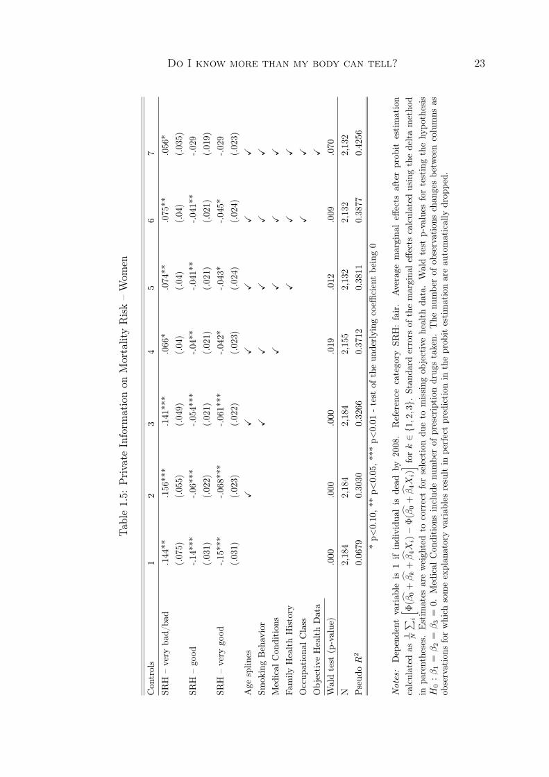
Average marginal effects of the SRH categories after estimating equation (1.1) arereported in tables 1.5 to 1.8. The first two tables display average marginal effects ofthe SRH categories on whether an individual dies within the next 10 years for men andwomen, respectively. Tables 1.7 and 1.8 display average marginal effects of SRH on anew diagnosis or recurrence of one of the major health conditions, heart disease, canceror stroke, in the next 8 years. All tables show results that are weighted to correct formissing data.7
Column 2 in each of the tables 1.5 and 1.6 is of specific interest. In additionto SRH the estimated models include the annuity underwriting controls. For bothgenders, all three SRH coefficients are significantly different from 0. Conditional onage, women in very good SRH in 1998 are 8 percentage points less likely to be deadin 2008 than women who rate their health as fair. Similarly, men in very good SRHin 1998 are 13 percentage points less likely to be dead in 2008 than men in fair SRH.When interpreting conditional information in SRH as private information these resultsshow evidence of a scope for adverse selection in annuity markets.
From left to right in tables 1.5 and 1.6 more control variables are added. Thelast columns report average marginal effects of the SRH categories when age, smokinginformation, medical conditions, family health history, social occupational class, andobjective health data are included as controls. The p-values of the Wald test forjoint significance indicate that for both genders the three SRH coefficients are stilljointly significantly different from 0 at the 10 percent significance level. The inclusionof the additional controls, however, and in particular the inclusion of the objectivelymeasured health information, leads to an attenuation in the average marginal effectsand to a reduction in the significance of the underlying SRH coefficients. Thoroughunderwriting, and in particular medical underwriting that includes blood tests andother objectively measured health data, is thus able to considerably reduce privateinformation about mortality risks.
Tables 1.7 and 1.8 show similar results for the diagnosis or re-diagnosis of a majorhealth condition within 8 years after the baseline interview. The results presented incolumn 1 of each table indicate that with no controls added in addition to SRH, thecoefficient of the three SRH categories are jointly significantly different from zero forwomen and men. When there is no individual underwriting, as in the case of group
7The estimation of the weights is described in the appendix to this chapter. Unweighted resultsdo not differ significantly from the weighted results.
Do I know more than my body can tell? 23
Table1.5:
Private
Inform
ationon
MortalityRisk–Wom
en
Con
trols
12
34
56
7SR
H–very
bad/
bad
.144**
.156***
.141***
.066*
.074**
.075**
.056*
(.075)
(.055)
(.049)
(.04)
(.04)
(.04)
(.035)
SRH
–go
od-.1
4***
-.06***
-.054***
-.04**
-.041**
-.041**
-.029
(.031)
(.022)
(.021)
(.021)
(.021)
(.021)
(.019)
SRH
–very
good
-.15***
-.068***
-.061***
-.042*
-.043*
-.045*
-.029
(.031)
(.023)
(.022)
(.023)
(.024)
(.024)
(.023)
Age
splin
esX
XX
XX
X
Smok
ingBehavior
XX
XX
X
Medical
Con
dition
sX
XX
X
Family
HealthHistory
XX
X
Occup
ationa
lClass
XX
Objective
HealthData
X
Waldtest
(p-value)
.000
.000
.000
.019
.012
.009
.070
N2,184
2,184
2,184
2,155
2,132
2,132
2,132
Pseud
oR
20.0679
0.3030
0.3266
0.3712
0.3811
0.3877
0.4256
*p<
0.10,*
*p<
0.05,*
**p<
0.01
-test
oftheun
derlying
coeffi
cientbe
ing0
Not
es:
Dep
endent
variab
leis
1if
individu
alis
dead
by2008.
Reference
category
SRH:fair.
Average
margina
leff
ects
afterprob
itestimation
calculated
as1 N
∑ i
[ Φ(β
0+βk
+β4X
i)−
Φ(β
0+β4X
i)] fo
rk∈{1,2,3}.
Stan
dard
errors
ofthemargina
leffe
ctscalculated
usingthedeltametho
din
parentheses.
Estim
ates
areweigh
tedto
correctforselectiondu
eto
missing
objectivehealth
data.Waldtest
p-values
fortestingthehy
pothesis
H0
:β1
=β2
=β3
=0.Medical
Con
dition
sinclud
enu
mbe
rof
prescription
drug
staken.
The
numbe
rof
observations
chan
gesbe
tweencolumns
asob
servations
forwhich
someexplan
atoryvariab
lesresultin
perfectprediction
intheprob
itestimationareau
tomatically
drop
ped.

Do I know more than my body can tell? 24
Table1.6:
Private
Inform
ationon
MortalityRisk–Men
Con
trols
12
34
56
7SR
H–very
bad/
bad
.274***
.228***
.212***
.104**
.102**
.094**
.064
(.064)
(.053)
(.051)
(.05)
(.049)
(.048)
(.045)
SRH
–go
od-.1
64***
-.096***
-.088***
-.062**
-.057**
-.054**
-.05**
(.034)
(.027)
(.026)
(.026)
(.026)
(.026)
(.025)
SRH
–very
good
-.203***
-.132***
-.119***
-.06**
-.054*
-.05*
-.035
(.033)
(.027)
(.026)
(.029)
(.029)
(.028)
(.028)
Age
splin
esX
XX
XX
X
Smok
ingBehavior
XX
XX
X
Medical
Con
dition
sX
XX
X
Family
HealthHistory
XX
X
Occup
ationa
lClass
XX
Objective
HealthData
X
Waldtest
(p-value)
.000
.000
.000
.003
.006
.011
.044
N1,766
1,766
1,766
1,766
1,766
1,766
1,766
Pseud
oR
20.1051
0.3206
0.3350
0.3961
0.4043
0.4088
0.4389
*p<
0.10,*
*p<
0.05,*
**p<
0.01
-test
oftheun
derlying
coeffi
cientbe
ing0
Not
es:
Dep
endent
variab
leis
1if
individu
alis
dead
by2008.
Reference
category
SRH:fair.
Average
margina
leff
ects
afterprob
itestimation
calculated
as1 N
∑ i
[ Φ(β
0+βk
+β4X
i)−
Φ(β
0+β4X
i)] fo
rk∈{1,2,3}.
Stan
dard
errors
ofmargina
leff
ects
calculated
usingthedeltametho
din
parentheses.
Estim
ates
areweigh
tedto
correctforselectiondu
eto
missing
objectivehealth
data.
Waldtest
p-values
fortestingthehy
pothesis
H0
:β1
=β2
=β3
=0.
Medical
Con
dition
sinclud
enu
mbe
rof
prescription
drug
staken.

Do I know more than my body can tell? 25
Table1.7:
Private
Inform
ationon
HealthRisk–Wom
en
Con
trols
12
34
56
78
SRH
–very
bad/
bad
.083
.137
.133
-.084
-.088
-.085
-.088
-.093*
(.144)
(.103)
(.1)
(.049)
(.05)
(.055)
(.049)
(.046)
SRH
–go
od-.1
82***
-.091**
-.091**
.011
.011
.01
.009
.011
(.052)
(.042)
(.042)
(.035)
(.035)
(.034)
(.035)
(.033)
SRH
–very
good
-.256***
-.167***
-.168***
-.024
-.023
-.02
-.022
-.011
(.052)
(.043)
(.043)
(.039)
(.039)
(.039)
(.039)
(.038)
Age
splin
esX
XX
XX
XX
Smok
ingBehavior
XX
XX
XX
Medical
Con
dition
sX
XX
XX
ServiceUse
XX
XX
Family
HealthHistory
XX
X
Occup
ationa
lClass
XX
Objective
HealthData
X
Waldtest
(p-value)
.000
.000
.000
.248
.238
.284
.273
.244
N1,572
1,572
1,572
1,572
1,572
1,572
1,572
1,571
Pseud
oR
20.0519
0.1381
0.1389
0.2551
0.2557
0.2636
0.2651
0.2801
*p<
0.10,*
*p<
0.05,*
**p<
0.01
-test
oftheun
derlying
coeffi
cientbe
ing0
Not
es:Dep
endent
variab
leis1ifindividu
aldiagno
sedor
re-diagn
osed
withheartdisease,
cancer
orstroke
inwaves
1,2or
3.Reference
category
SRH:
fair.Average
margina
leff
ects
afterprob
itestimationcalculated
as1 N
∑ i
[ Φ(β
0+βk
+β4X
i)−
Φ(β
0+β4X
i)] fo
rk∈{1,2,3}.
Stan
dard
errors
ofmargina
leffe
ctscalculated
withthedeltametho
din
parentheses.
Estim
ates
areweigh
tedto
correctforselectiondu
eto
missing
objectivehealth
data
andattrition.
Waldtest
p-values
fortestingthehy
pothesisH
0:β1
=β2
=β3
=0.Medical
Con
dition
sinclud
enu
mbe
rof
prescription
drug
staken.
The
numbe
rof
observations
chan
gesbe
tweencolumns
asob
servations
forwhich
someexplan
atoryvariab
lesresult
inpe
rfectprediction
intheprob
itestimationareau
tomatically
drop
ped

Do I know more than my body can tell? 26
Table1.8:
Private
Inform
ationon
HealthRisk–Men
Con
trols
12
34
56
78
SRH
–very
bad/
bad
.106
.068
.051
-.055
-.047
-.028
-.031
-.025
(.119)
(.108)
(.104)
(.064)
(.064)
(.062)
(.06)
(.056)
SRH
–go
od-.0
68-.0
51-.0
51.009
.009
.012
.012
.023
(.063)
(.062)
(.059)
(.043)
(.043)
(.041)
(.041)
(.038)
SRH
–very
good
-.119*
-.107*
-.112*
-.026
-.024
-.008
-.012
-.003
(.067)
(.067)
(.065)
(.047)
(.047)
(.045)
(.045)
(.041)
Age
splin
esX
XX
XX
XX
Smok
ingBehavior
XX
XX
XX
Medical
Con
dition
sX
XX
XX
ServiceUse
XX
XX
Family
HealthHistory
XX
X
Occup
ationa
lClass
XX
Objective
HealthData
X
Waldtest
(p-value)
.093
.170
.180
.652
.695
.893
.849
.771
N1,240
1,240
1,240
1,240
1,240
1,240
1,240
1,239
Pseud
oR
20.0224
0.0650
0.0784
0.2217
0.2243
0.2495
0.2520
0.2746
*p<
0.10,*
*p<
0.05,*
**p<
0.01
-test
oftheun
derlying
coeffi
cientbe
ing0
Not
es:Dep
endent
variab
leis1ifindividu
aldiagno
sedor
re-diagn
osed
withheartdisease,
cancer
orstroke
inwaves
1,2or
3.Reference
category
SRH:
fair.Average
margina
leff
ects
afterprob
itestimationcalculated
as1 N
∑ i
[ Φ(β
0+βk
+β4X
i)−
Φ(β
0+β4X
i)] fo
rk∈{1,2,3}.
Stan
dard
errors
ofmargina
leff
ects
calculated
withdeltametho
din
parentheses.
Estim
ates
areweigh
tedto
correctforselectiondu
eto
missing
objectivehealth
data
andattrition.
Waldtest
p-values
fortestingthehy
pothesisH
0:β1
=β2
=β3
=0.Medical
Con
dition
sinclud
enu
mbe
rof
prescription
drug
staken.
The
numbe
rof
observations
chan
gesbe
tweencolumns
asob
servations
forwhich
someexplan
atoryvariab
lesresult
inpe
rfectprediction
intheprob
itestimationareau
tomatically
drop
ped.

Do I know more than my body can tell? 27
health insurance, there is thus private information and therefore scope for adverseselection.
The inclusion of additional controls from left to right in tables 1.7 and 1.8 results ina reduction in the information in SRH. For both genders, the inclusion of self-reportedmedical conditions and the number of prescription drugs taken as shown in columns 4of the respective tables leaves no additional explanatory power in SRH for the diagnosisor re-diagnosis of a major health condition. Taking information in SRH on a futurediagnosis of a major condition as private information, the results indicate that medicalunderwriting is a crucial determinant of the degree of private information left in privatehealth insurance markets.
Overall, the results present evidence that medical underwriting, and in particularunderwriting including medical examinations significantly reduces private informationas captured by SRH. While I find evidence that private information on mortality risksremains even with stringent underwriting, I find no evidence of private information onhealth risks when stringent underwriting is employed. There is evidence, however, forprivate information on health risks when no or scarce information is used in underwrit-ing. Differences in adverse selection between group health insurance markets withoutindividual underwriting and individual health insurance with stringent individual un-derwriting can therefore be reconciled precisely by the differences in underwriting.
1.6 Robustness Analyses
In this section, I present different sensitivity analyses. First, the time horizon withinwhich the realization of risk can occur is shortened to 4 years to investigate whetherindividuals have more information on risks in a shorter term. Second, subjective lifeexpectancy is included in the analysis instead of SRH, as it might be a better proxy forprivate information on future health events. Third, I analyze how well the underwrit-ing controls help to predict the outcomes to gauge the scope for private informationindependent of the different proxies for individual information.
Table 1.9 reports the average marginal effects of the three SRH categories whenthe dependent variables capture the realization of risk within the next 4 years. Resultsfor women are displayed in the upper panel, results for men in the lower panel. Thedependent variable in columns 1 and 2 is an indicator for whether an individual is deadby ELSA wave 1. In columns 3 and 4 the dependent variable is an indicator for whetheran individual reports a diagnosis or recurrence of a major health condition in wave 1.The first column for each event includes a limited set of control variables in addition to

Do I know more than my body can tell? 28
Table 1.9: Robustness – Event by 2002
Mortality Risk Health RiskAnnuities Life Insurance Group HI Individual HI
1 2 3 4Women
SRH – very bad/bad .094*** .036 .114 -.032(.037) (.025) (.163) (.043)
SRH – good -.022 -.002 -.176*** -.003(.016) (.014) (.055) (.029)
SRH – very good -.022 .002 -.22*** -.004(.016) (.016) (.055) (.033)
Wald test (p-value) 0.000 0.407 0.000 0.917N 2,184 2,054 1,558 1,557Pseudo R2 0.2398 0.4303 0.0660 0.3427Men
SRH – very bad/bad .103** -.004 .136 .005(.052) (.031) (.116) (.051)
SRH – good -.036* -.015 -.079 -.014(.02) (.02) (.055) (.033)
SRH – very good -.069*** -.031 -.139** -.076**(.02) (.022) (.057) (.034)
Wald test (p-value) 0.000 0.582 0.008 0.08N 1,766 1,690 1,222 1,204Pseudo R2 0.2094 0.3719 0.0507 0.3442
* p<0.10, ** p<0.05, *** p<0.01 - test of the underlying coefficient being 0
Notes: Average marginal effects after probit estimation and their standard errors in parentheses.Different columns include different sets of control variables. Column Annuities includes age splines,Life Insurance includes age splines, smoking information, medical conditions, number of prescriptiondrugs taken, family health history, social occupational class, and objective health data, Group HIincludes no controls in addition to SRH, and Individual HI includes the same variables as Life Insuranceplus use of medical services. Results are weighted to correct for missing data.

Do I know more than my body can tell? 29
SRH, the second column includes the most comprehensive set of underwriting controls.Similarly to the results of the main analysis, there is significant information in SRH
on dying within the next 4 years and on being diagnosed with a major health conditionwithin the next 4 years when only limited sets of underwriting controls are included.Including the most comprehensive set of the life insurance underwriting controls, XLife,eliminates any information in SRH on the 4 year mortality risk. With respect to the 4year health risk, however, column 4 of table 1.9 presents evidence that at least for mensome information remains in SRH even when the set of individual health insurancecontrols, XIndividualHI , is included. SRH thus may contain more information in theshorter term.
In the upper panel of table 1.10 results are reported with subjective life expectancyreplacing SRH in equation (1.1) as proxy for private information.8 Subjective lifeexpectancy is only available in ELSA starting from wave 1. The earliest wave thatcontains subjective life expectancy and objectively measured health data is wave 2. Ithus use wave 2 as baseline in this robustness analysis. The dependent variables arewhether an individual is dead by 2008 and whether an individual reports a diagnosisor recurrence of heart disease, cancer or stroke in wave 3. As wave 2 was elicited in2006, the time horizon within which the risks can materialize is 2 years.
For means of comparison results using SRH in the 2006 wave of ELSA as proxyfor individual information are reported in the lower panel of table 1.10. Columns 1and 2 report average marginal effects on the probability of being dead in 2008 formen and women, respectively, columns 3 and 4 report average marginal effects onthe probability of being diagnosed with heart disease, cancer, or stroke for the twogenders. Only results with the most comprehensive sets of additional control variablesare presented in order to gauge how much private information there is in the case ofstringent underwriting.
The results presented in the upper panel of table 1.10 indicate that subjective lifeexpectancy contains information on whether individuals die or survive the next 2 yearseven when a comprehensive set of additional controls is included. Column 3 and 4present evidence that there is no significant information in subjective life expectancyfor an onset of a major health condition within the next 2 years. SRH in 2006, onthe contrary, contains information on dying in the next two years only for men andon the onset of a major health condition for both genders. These results suggest thatsubjective life expectancy contains more information on mortality risks, while SRH is
8Subjective life expectancy in ELSA is elicited with the question “What are the chances that youwill live to be x or more?” Where x depends on the individual’s age at the time of the interview. Theaverage time horizon for this question in the estimation sample is 15 years.

Do I know more than my body can tell? 30
Table 1.10: Robustness – Subjective Life Expectancy
Mortality Risk Health RiskMen Women Men Women1 2 3 4
Subjective Life ExpectancyProbability of surviving – 0− 24% -.032 .004 .049 .028
(.020) (.014) (.037) (.036)Probability of surviving – 50− 74% -.056*** -.023** -.019 .008
(.019) (.012) (.030) (.029)Probability of surviving – 75− 100% -.054*** -.017 -.016 -.025
(.020) (.014) (.031) (.030)Wald test (p-value) 0.003 0.0156 0.0968 0.1358N 2,136 2,504 1,909 2,315Pseudo R2 0.3073 0.2814 0.2472 0.2838
Self-Rated HealthSRH – bad/fair .046*** .010 .027 .071***
(.016) (.009) (.028) (.024)SRH – very good -.011 -.012 -.026 .007
(.010) (.007) (.022) (.019)SRH – excellent .005 -.007 -.060** -.015
(.016) (.011) (.028) (.025)Wald test (p-value) 0.004 0.1312 0.0920 0.012N 2,135 2,504 1,908 2,315Pseudo R2 0.3081 0.2734 0.2464 0.2866
* p<0.10, ** p<0.05, *** p<0.01 - test of the underlying coefficient being 0
Notes: Average marginal effects after probit. Standard errors in parentheses. Dependent variablewhether an individual is dead by the year 2008 for mortality risk, and whether there was an onsetor recurrence of heart disease, cancer and/or stroke for health risk. Explanatory variables are takenfrom ELSA wave 2. Reference category of subjective life expectancy is 25-49%. SRH measured onthe US scale in wave 2, good SRH, the middle category, chosen as reference. Control variables in eachestimation are: age splines, smoking information, medical conditions, number of prescription drugstaken, family health history, and objective health data. Results are weighted to correct for missingobjective health data using weights provided in ELSA.

Do I know more than my body can tell? 31
better suited to predict health risks – at least in the short run. Whether this findingalso holds in the longer term, is subject to additional analyses that will be possibleonce a longer follow-up period is available in ELSA.
SRH and subjective life expectancy are only proxies for individual informationon future health risks. Individuals could have information on the insured risks that isneither included in SRH nor subjective life expectancy nor in the verifiable underwritingcontrols. In order to gauge the scope for private information independent of a proxy forindividual information, I estimate probit models where only the underwriting controlsare included
yj∗i = γj0 + γj1Xai + ηji (1.2)
yji = I(yj∗i > 0).
Xai represents the vectors of the respective most comprehensive sets of underwritingcontrols for both dependent variables, yMi and yDi . The better these comprehensive setsof underwriting controls help to predict the future realization of the insured risk, thebetter the insurer will be able to discriminate between risk types based on the collectedinformation. The less scope thus remains for private information.
In order to analyze how well models explain the variation in binary dependent vari-ables, often the percent of correctly predicted observations is reported. This approachinvolves predicting the probability, P r(yji = 1|Xai), for each individual and choosingsome cutoff above which the researcher assumes that the predicted probability corre-sponds to predicting a 1 and below which it corresponds to predicting a 0. One canthen calculate how many of the actual ones and how many of the actual zeros arecorrectly predicted by the model. It is not clear, however, what the optimal choice ofcutoff is (see Wooldridge, 2010, p. 573f. for a discussion).
In order to avoid the choice of a specific cutoff, I display the distributions of thepredicted probabilities by the values of the actual outcome variable. For example,figure 1.3 contains the cumulative distribution functions of P r(yDi = 1|Xai) for menwho are still alive in 2008 and for men who are dead by 2008. Figure 1.4 displays thesame for women, and figures 1.5 and 1.6 display the respective cumulative distributionfunctions of P r(yMi = 1|Xai) for men and women, respectively.
For any cutoff probability, the figures show how large the share is of individualsin the two outcome groups with a predicted probability below or above the respectivecutoff. In figure 1.3 with a cutoff at P r(yDi = 1|Xai) = 20%, for example, 80% of menwho are still alive in 2008 have a predicted probability that is lower than the cutoff,

Do I know more than my body can tell? 32
Figure 1.3: Predicted Probability Death - Men
Figure 1.4: Predicted Probability Death - Women
and 80% of men who are dead by 2008 have a predicted probability that is higher thanthe cutoff. If an insurer thus set a cutoff at 20% and treated every individual with apredicted probability below this cutoff as low risk and every individual with a predictedprobability above this cutoff as high risk, it would correctly classify 80% of men. Figures1.4 to 1.6 display similar patterns. Based on the underwriting controls it thus seemsto be possible to discriminate rather accurately between individuals who experience anevent in the future and individuals who do not experience the respective event. This

Do I know more than my body can tell? 33
Figure 1.5: Predicted Probability Major Condition - Men
Figure 1.6: Predicted Probability Major Condition - Women
provides further evidence that there is not a lot of room for private information in thedifferent insurance markets when stringent underwriting is employed.
Overall, the analyses presented in this section strengthen the intuition that stringentunderwriting helps to reduce private information in the markets for life insurance andindividual health insurance. At least for the individuals’ information on the risksinsured in health insurance markets, SRH seems to be a better proxy than subjectivelife expectancy. Furthermore, there is evidence that even independent of the choice

Do I know more than my body can tell? 34
of a proxy for individuals’ information on their health risks, little scope for privateinformation remains with stringent underwriting.
1.7 Conclusion
Mixed empirical evidence on adverse selection in different insurance markets standsin contrast to robust predictions of the existence of adverse selection in theoreticalmodels. This divergence has engendered research that tries to reconcile theoreticaland empirical results. This chapter focuses on one possible explanation for the mixedfindings in the empirical literature: different scopes of adverse selection in differentinsurance markets. In insurance markets in which insurance companies collect a lot ofinformation about their applicants and use this information for underwriting, privateinformation might not exist and thus there might be no scope for adverse selection.
In this study, I focus on the markets for life insurance, annuities and health insur-ance. Private information in these markets is detected by using information in SRHon dying in the next years and on future diagnoses of diseases. Different verifiablemeasures are included as controls in addition to SRH to imitate different types of in-formation used in underwriting in the different insurance markets. The informationthat remains in SRH when the different sets of underwriting controls are included isinterpreted as private information in the different insurance markets.
The analysis employs data from ELSA, one of the rare longitudinal data sets thatprovides objectively measured health data. The data set allows to mimic medicalunderwriting with greater precision than is typically possible with data from otherpopulation surveys that only include self-reported health information. As thoroughunderwriting that includes outcomes of medical examinations is typically conductedin life insurance markets and private individual health insurance markets, ELSA’sobjectively measured health data is particularly valuable for my analysis.
Dying within the next 10 years is significantly related to SRH at baseline whenonly information on age and sex is additionally included in the analysis. When med-ical information and in particular objectively measured health data are additionallyincluded, however, the predictive power of SRH for death or survival is considerablyreduced. Similarly, there is significant information in SRH for the diagnosis or recur-rence of a major health condition in the next 8 years with only limited controls. Theinclusion of medical information reduces the amount of information contained in SRHto insignificant levels.
Interpreting the remaining information in SRH when underwriting controls are

Do I know more than my body can tell? 35
included in the analyses as private information, I thus find evidence for private infor-mation on mortality risk and health risk if insurance companies do not use medicalinformation for underwriting. When medical underwriting is conducted, however, theprivate information and thus the scope for adverse selection is reduced in life insuranceand eliminated in health insurance markets.
These findings can help to reconcile differences in the evidence of adverse selectionbetween life insurance and annuity markets and between group and individual privatehealth insurance markets. Only limited information is used for underwriting in grouphealth insurance and annuity markets and these markets are found to suffer fromadverse selection. In individual health and life insurance markets medical underwritingis typically performed and there is little evidence for adverse selection in these markets.Differences in the information used for underwriting in the different markets – partlyresulting from different underwriting regulations – leave different amounts of privateinformation and thus different scopes for adverse selection.
My results in turn indicate that employing stringent underwriting in group healthinsurance and annuity markets could reduce and possibly eliminate adverse selectionin these markets. Recent research finds that adverse selection reduces welfare in themarket for annuities (Einav et al., 2010b) and in health insurance markets (Bundorfet al., 2008). A question that my analysis cannot answer, however, is how stringentunderwriting would affect overall welfare in these markets. On the one hand, strin-gent underwriting might increase welfare by eliminating welfare losses resulting fromadverse selection. On the other hand, it might at the same time reduce welfare inother dimensions. For example, in the case of short-term insurance contracts whereindividuals have to buy insurance coverage repeatedly, repeated stringent underwritingwould introduce an additional risk to the existing health-related risks, namely the riskof becoming a ‘high risk’ in the future. If there is no insurance to insure against thisadditional risk, a “welfare loss from incomplete insurance contracts” will arise (Cutlerand Zeckhauser, 2000, p. 627). Whether stringent underwriting increases or decreaseswelfare thus depends on the specific institutional setting.

Do I know more than my body can tell? 36
Appendix: Inverse Probability Weighting
In order to correct for item non-response and attrition I use inverse probability weight-ing. To correct for the two selection mechanisms simultaneously, I estimate the jointprobability of availability of all objective health measures in wave 0, (h = 1), and noattrition after wave 0, (a = 1), using a bivariate probit model.
The crucial assumption for consistency with this approach is conditional indepen-dence
Pr(a = 1, h = 1|y, SRH,XIndividualHI , d) = Pr(a = 1, h = 1|SRH,Z, d)
where Z ⊂ XIndividualHI , and XIndividualHI is the most comprehensive set of under-writing controls. Z includes all variables in XIndividualHI except for the objectivelymeasured health data. d is a vector of additionally included control variables.
The conditional independence assumption would be invalidated by the existenceof unobservables that influence both – selection and the outcome y. The variablesincluded in d thus not only have to be significant predictors of attrition and item non-response but also have to be related to y in order to attenuate the worry of unobservableinfluences. Potential candidates for inclusion in d are health-related variables that arenot used by insurance companies for underwriting and are therefore not included inthe different sets of control variables X.
In my analysis, d includes information on marital status, activity status, race, thehousehold’s economic situation, survey participation behavior of other survey membersin the same household, the individual’s survey participation behavior in other parts ofthe survey in wave 0, and information on the situation during the interview.
Separate bivariate probit models are estimated for men and women. The coefficientsare displayed in table 1.11. Many of the variables included in d significantly affectselection. Furthermore, the two selection mechanisms are positively correlated forboth genders. An individual who is more likely to stay in the survey is also more likelyto have a nurse visit and a blood sample taken. This could reflect an unobserved likingfor surveys.
The results in table 1.11 are used to predict Pr(a = 1, h = 1|SRH,Z, d) andPr(h = 1|SRH,Z, d) for each individual. 1
P r(a=1,h=1|SRH,Z,d)is used as a weight in
estimation when the dependent variables is an indicator of a diagnosis or reccurence ofa major health condition. Whether an individual dies or not is observed irrespectiveof attrition, therefore 1
P r(h=1|SRH,Z,d)is used as a weight in the estimations for private
information on mortality risk.

Do I know more than my body can tell? 37
Table 1.11: Selection Mechanisms – Bivariate Probit
Women Mena h a h
Completed other 0.197 (0.167) 0.377** (0.157) -0.146 (0.202) 0.465*** (0.180)Partner a=1 2.360*** (0.067) 0.262*** (0.049) 2.468*** (0.071) 0.235*** (0.053)Partner h=1 -0.154** (0.064) 0.638*** (0.049) -0.112* (0.067) 0.603*** (0.051)Interviewed alone 0.233*** (0.063) 0.103* (0.055) 0.599*** (0.080) 0.058 (0.064)HH size -0.064** (0.030) 0.004 (0.026) -0.035 (0.035) 0.009 (0.027)Rent home -0.050 (0.058) 0.016 (0.052) -0.100 (0.074) -0.131** (0.063)Married -0.73*** (0.076) -0.245*** (0.067) -0.609*** (0.096) -0.295*** (0.081)Widowed -0.034 (0.075) -0.006 (0.072) 0.310*** (0.113) 0.081 (0.106)White 0.118 (0.125) 0.045 (0.115) -0.242 (0.153) 0.023 (0.129)Retired -0.018 (0.068) 0.016 (0.059) -0.17 (0.213) -0.195 (0.186)Unemployed 0.623*** (0.235) 0.082 (0.188) -0.484* (0.254) -0.462** (0.221)Working -0.039 (0.075) 0.036 (0.061) -0.273 (0.200) -0.299* (0.176)SRH X X X X
Age splines X X X X
Smoking behavior X X X X
Medical conditions X X X X
Service use X X X X
Family history X X X X
Occupational class X X X X
ρ 0.233*** (0.029) 0.149*** (0.035)N 4,648 3,556
* p<0.10, ** p<0.05, *** p<0.01
Notes: Coefficients after bivariate probit analysis displayed. Standard errors in parentheses. a isequal to 1 if an individual is observed at least once after ELSA wave 0, h is equal to 1 if all objectivelymeasured health variables are observed for an individual.

Chapter 2
Do they know what’s at risk?Health Risk Perception Among theOverweight and Obese
2.1 Introduction
Excess body weight is a risk factor for various diseases. In particular, it increases therisks of type 2 diabetes, cardiovascular disease, several cancers, arthritis, and psycho-logical problems (Haslam and James, 2005; Dixon, 2010). Today, more than 70% ofUS adults are overweight or obese, meaning that they have a Body Mass Index (BMI)between 25 and 30, or of at least 30, respectively.1 Furthermore, a large share of USmedical expenditures is caused by excess weight (Cawley and Meyerhoefer, 2010).
While the causes of excess body weight are multifactorial, body weight depends oneach individual’s behavior. Individuals can choose how many calories they consumeand whether they engage in activities with high or low calorie expenditure, for examplethey can choose whether they are physically active.
Attempts to help individuals lose weight have shown limited success. In a meta-analysis McTigue et al. (2003) find that various interventions only promoted modestweight loss. One possible explanation for this is that individuals who carry excessweight are not aware of the danger that this weight poses to their health. Gregoryet al. (2008) accordingly find that individuals who do not rate their weight as a healthrisk are less likely to engage in weight loss activities than individuals who rate theirweight as a health risk.
1The BMI is measured as weight(kg)height2(m2) . Information on overweight and obesity in the US from the
National Health and Nutrition Examination Survey (NHANES), 2007/08.

Do they know what’s at risk? 39
In this chapter we analyze whether middle-aged individuals in the US with excessbody weight underestimate their personal risks of diabetes, stroke, heart attack, lungdisease, hypertension and arthritis or rheumatism. Health risk perceptions among over-weight and obese individuals have been studied by Kan and Tsai (2004) and Gregoryet al. (2008). Our analysis contributes to this literature by measuring individual riskperceptions in a different way. In particular, while Kan and Tsai (2004) and Gregoryet al. (2008) use information on individual risk perception stemming from qualitativequestions, we ask individuals about numerical probabilities of developing different dis-eases in the future. An advantage of our numerical subjective measures is that theycan be compared to objective probabilities. This allows us to investigate how accurateindividual risk perceptions are.
Our data on subjective disease probabilities comes from the American Life Panel(ALP), a panel study administered by RAND. In an ongoing survey in the ALP thatwent into the field in the summer of 2010 we ask the survey participants to assesstheir chances of developing different diseases in the next 5 years on a 0-100 scale.In the design of these health expectations questions we follow Manski (2004) who alsoprovides a general assessment of the validity of similar expectation questions in differentdomains, such as stock market returns and returns to schooling.
In order to gauge how well individuals are informed about their health risks weestimate objective probabilities of developing the different diseases in the next 5 years.In the estimation of these objective disease probabilities we follow Khwaja et al. (2009)who conduct a similar analysis on risk perception among smokers. More specifically, weestimate relationships between individual characteristics and future disease onsets inthe Health and Retirement Study (HRS). Under the assumption that these relationshipsare the same in the ALP today as they were in the HRS a few years ago, we use theestimates from the HRS to predict the probabilities of disease onsets for individuals inthe ALP.
While not the main focus of our analysis, we use the subjective and objectivedisease probabilities in the ALP data to replicate the study by Khwaja et al. (2009)on the accuracy of risk perception among current and former smokers. The results arepresented in the appendix to this chapter. Essentially, we are able to reproduce theirfindings that current and former smokers do not underestimate the different healthrisks.
Obese individuals in the ALP, on the contrary, underestimate certain health risks.In particular, we find evidence that obese individuals underestimate the risks of de-veloping arthritis, diabetes and hypertension within the next 5 years. The results for

Do they know what’s at risk? 40
arthritis are robust to changes in the calculation of the objective risks. The risks ofdeveloping other diseases, such as a heart attack or a stroke, however, are significantlyoverestimated by the overweight and obese. As the objective risks of developing thesediseases are relatively small on average, even among obese individuals, this overesti-mation corresponds to results from other studies that find that individuals tend tooverestimate low probability events (see e.g. Lichtenstein et al., 1978).
The significant underestimation of the risks of arthritis, diabetes and hypertensionamong the obese indicates that there is a need for health education in this group.While health education programs targeted at the overweight and obese will probablynot suffice to fully control the obesity epidemic, our results indicate that there is roomfor health education programs to help these individuals make better informed lifestylechoices.
The chapter is structured as follows. Section 2 summarizes the related literature.Section 3 describes the two data sets that we use in this analysis. In Section 4 theempirical methods are explained. Section 5 presents the results. Section 6 explores therobustness of the results, and Section 7 concludes.
2.2 Related Literature
Our analysis is closely related to two strands of literature. The first strand focuses di-rectly on risk perceptions among the overweight and obese. The second strand analyzesrisk perception among smokers.
The different studies that analyze risk perception among the overweight and obesefocus primarily on the relationship between risk knowledge and the tendency to beoverweight or obese rather than on the accuracy of the risk knowledge. Kan and Tsai(2004) find that there is a relationship between individuals’ perception of health risksresulting from excess weight and the tendency to carry excess weight in Taiwanese men.In particular, men with very high BMI seem to be less aware of obesity-related healthrisks. For women, the authors find no relationship between health risk perceptionand BMI. Similarly, Gregory et al. (2008) find that overweight and obese adults inthe US who do not perceive their weight as a risk factor are less likely to engage inweight lowering activities. Furthermore, the authors show that significant fractions ofoverweight and obese adults do not agree to the statement that their weight is a healthrisk. This suggests a lack of health knowledge on weight as a risk factor. However,the question that measures health knowledge is targeted at overall health risks and isthus very general. It does not allow to distinguish between risks of different diseases.
Do they know what’s at risk? 41
Moreover, because of the question’s qualitative nature it is not clear how accurateindividual risk perceptions are.
Analyses of risk perception among smokers have focused on the accuracy of the riskperception. Viscusi (1990) pioneered this type of analysis in economics by comparingindividuals’ assessments of the probability that smokers get lung cancer because theysmoke with objective measures of this probability. His results indicate that smokersand non-smokers significantly overestimate the risk of lung cancer due to smoking.Viscusi and Hakes (2008) extend the earlier analysis to the accuracy of individuals’assessments of the probability that smokers die from lung cancer, heart disease, or anyother illness because they smoke, and to the accuracy of loss in life expectancy due tosmoking. In line with Viscusi’s earlier findings their results indicate that smokers andnon-smokers overestimate the risk of dying from smoking and the years of life lost dueto smoking when compared to the risks of dying from smoking and life years lost asreported in the medical literature. As smokers overestimate these risks less than non-smokers, the results are consistent with the idea that higher risk perceptions protectindividuals from smoking.
While Viscusi (1990) and Viscusi and Hakes (2008) study perceptions of generalrisks of smoking, i.e. individuals are asked about the risks of a hypothetical smoker,Schoenbaum (1997) and Khwaja et al. (2009) analyze the accuracy of risk estimatesconcerning the individuals’ personal risks. Schoenbaum (1997) compares individualexpectations of reaching age 75 measured in the HRS with actuarial predictions basedon life tables for the groups of never smokers, former smokers, current light smokers,and current heavy smokers. Heavy smokers are found to significantly overestimatethe probability of reaching age 75, while the other groups have about accurate riskperceptions. In Khwaja et al. (2009), individual expectations of reaching age 75 andexpectations of getting certain diseases until the age of 75 are compared with individualobjective risk estimates for each event. The objective risk estimates are based on therelationship between individual characteristics and disease probabilities as estimatedfrom the HRS. Their results indicate that smokers do not underestimate disease andmortality risks.
2.3 Data
The analysis in this chapter is based on two data sets. The main analysis is con-ducted with data from the American Life Panel (ALP) in which we elicited subjectiverisk expectations. Data from the Health and Retirement Study (HRS) is used in the

Do they know what’s at risk? 42
calculation of objective health risks for individuals in the ALP.The HRS was started in 1992 as a representative study of the US non-institutiona-
lized population born between 1931 and 1941. Blacks, Hispanics and residents ofFlorida were oversampled. Sampling weights are provided to correct for this oversam-pling. Data was collected every two years since 1992. The last currently available datais from 2008. In later waves, additional cohorts were added to the HRS. In particu-lar, in 1998 the “children of depression (CODA)” cohort (born 1924-1930) and the “warbaby” cohort (born 1942-1947) were added to the data. We use the 1992 HRS wave andfollow-up until 2008 to estimate prediction models for onset of diseases for a populationaged 50-62. As a robustness check we also use a later HRS wave as a baseline year inthe risk prediction models. In particular, we use the 1998 wave. The integration ofadditional cohorts in this wave allows to focus the analysis on a representative samplefor the same age group (50-62 year-olds) as when the 1992 wave is used as baseline.
The second data source is the American Life Panel (ALP), an internet survey ofabout 3,200 American adults administered by RAND (see http://rand.org/labor/roybalfd/american_life.html for a full description). We implemented a survey in theALP that went into the field in July 2010 and is still ongoing. The focus of our surveylies primarily on eliciting individuals’ subjective expectations of developing certaindiseases in the future. We elicit the expectations as numerical probabilities with thequestion “What do you think is the percent chance that you will develop, or re-developif you have already been diagnosed with it, the following conditions in the next 5 yearsand ever in you lifetime?".2 The question is preceded by a text that explains theprobability scale from 0 to 100, where 0 means that there is absolutely no chance, or 0percent, and 100 means the event is absolutely sure to happen, or 100 percent. Similartypes of questions on survival expectations have proven useful in eliciting subjectiveprobabilities that have predictive power for actual outcomes (see Hurd, 2009, for asummary).
In addition to the subjective expectations we elicited information on risk factorsfor the specific diseases, including questions on co-morbidities, family history, andlifestyle. 915 of the surveyed individuals in our sample are between 50 and 62 yearsold at the time of the survey. While the ALP is not a representative sample for the USpopulation, RAND provides weights to make it comparable to the Current Population
2Individuals who report that they have been diagnosed with chronic diseases, such as diabetesor chronic lung disease, are not asked about their chances of developing the specific conditions. Forconditions that may relapse, like a stroke or a heart attack, all individuals are asked about the chancesindependent of their prior history of the disease. In this chapter, we focus on the 5 year risks. In afollow-up analysis, we plan to also investigate the accuracy of the lifetime risk perceptions.

Do they know what’s at risk? 43
Survey. These weights are used in all following analyses.
Table 2.1: Descriptive Statistics
HRS 1992 ALPVariable Mean SD Mean SDSelf-rated health
Excellent 0.24 0.43 0.08 0.32Very Good 0.30 0.47 0.41 0.61Good 0.27 0.44 0.33 0.58Fair 0.13 0.34 0.15 0.44Poor 0.07 0.26 0.03 0.22
BMINormal weight (BMI<25) 0.35 0.48 0.27 0.55Overweight (25≤BMI<30) 0.41 0.49 0.36 0.59Obese 1 (30≤BMI<35) 0.16 0.37 0.22 0.51Obese 2 (35≤BMI<40) 0.04 0.20 0.07 0.31Obese 3 (BMI≥40) 0.02 0.14 0.08 0.33
Smoking StatusCurrent Smoker 0.27 0.44 0.21 0.50Former Smoker 0.37 0.48 0.32 0.57Never Smoker 0.36 0.48 0.47 0.62
DemographicsAge 55.56 3.25 55.55 4.52White 0.86 0.345 0.84 0.45Male 0.48 0.50 0.49 0.62Married 0.74 0.44 0.68 0.57
EducationLess than High School 0.23 0.42 0.06 0.28High School or equiv 0.39 0.49 0.33 0.58Some College 0.20 0.40 0.30 0.56BA or equiv 0.11 0.31 0.20 0.49More than BA 0.08 0.27 0.12 0.40
N 9,793 906
Notes: Sampling weights used in estimation of means and standard deviations (SD).
In table 2.1 weighted means and standard deviations of relevant health variables,risk factors and demographics are displayed for individuals aged 50 to 62 in the ALPdata. For means of comparison, descriptives are also displayed for the HRS 1992sample.
While the HRS and ALP samples seem to be similar in age and sex, there aredifferences in BMI categories, smoking status, and education. Less of the individuals

Do they know what’s at risk? 44
in the ALP sample are current or former smokers, but more of them are overweight orobese. These differences align with changes in the prevalence of smoking and obesityover the last decades. While the fraction of smokers decreased, the fraction of individ-uals with excess weight increased.3 The individuals in the ALP 2010 are furthermoreon average better educated than the individuals in the HRS in 1992. This could reflectthe steady advance in educational accomplishments in the US.4 For the results of ouranalysis the differences in individual characteristics between the samples do not matteras long as the relationship between the individual characteristics and the probabilitiesof developing different diseases in the future are constant over time. We shed light onthe question how strong this assumption is in the aforementioned robustness check inwhich we use a later HRS wave as baseline.
The first two columns of table 2.2 display averages and standard errors of thesubjective disease probabilities in the ALP for individuals who are between 50 and62 years old. For each disease, only individuals are included who do not report everhaving been diagnosed with the respective disease. In addition to the overall averages,means of the subjective probabilities are shown for the different BMI categories. It canbe observed that the overall means vary between conditions. The means range froman 8 percent risk of developing lung disease in the next 5 years to a 21 percent risk ofdeveloping arthritis or rheumatism. Furthermore, the average risks vary by categoriesof BMI. For example, individuals with a BMI between 30 and 35 on average rate theirrisk of diabetes in the next 5 years more than 2 times as high as individuals with a BMIlower than 25. For none of the conditions, however, there is a clear graded relationshipbetween average subjective risk and BMI.
2.4 Estimation Methods
In order to evaluate the accuracy of individuals’ subjective beliefs on different riskswe construct objective risks of getting different diseases in the next 5 years for everyindividual in the ALP. In a second step, we analyze whether the difference between thesubjective and objective risk is related to the individuals’ BMI.
3See National Center for Health Statistics (2010), page 24ff. for trends in smoking and obesity inthe US.
4The trend in educational attainment can be seen in data from the U.S. Census available atwww.census.gov/hhes/socdemo/education/data/cps/historical/index.html. The data shows that in1992 25.7% of the 35 to 55 year old individuals and 14.2% of the individuals aged 55 or above inthe US had finished their education with 4 years of college or more compared to 27.3% of the youngerand 26.4% of the older group in 2009.

Do they know what’s at risk? 45
Table 2.2: Subjective and Objective Risk
Subjective Risk Objective Risk
Mean SE Mean SE
Diabetes Total 10.58 0.72 5.34 0.24
BMI<25 7.14 1.04 1.22 0.05
25≤BMI<30 10.45 1.09 3.89 0.08
30≤BMI<35 15.15 2.04 8.79 0.25
35≤BMI<30 10.48 1.64 12.76 0.69
BMI≥40 14.44 3.81 17.62 0.58
Stroke Total 12.37 0.81 1.91 0.06
BMI<25 10.05 1.37 1.41 0.08
25≤BMI<30 11.28 1.06 1.52 0.07
30≤BMI<35 14.88 2.12 2.12 0.12
35≤BMI<40 18.44 3.50 2.47 0.23
BMI≥40 13.37 3.75 4.54 0.40
Lung Disease Total 8.14 0.62 2.55 0.11
BMI<25 7.71 1.21 2.39 0.23
25≤BMI<30 8.70 1.18 2.19 0.14
30≤BMI<35 9.00 1.19 2.70 0.24
35≤BMI<40 6.22 1.32 3.37 0.41
BMI≥40 5.95 1.18 3.84 0.39
Heart Attack Total 13.07 0.79 3.13 0.11
BMI<25 9.90 1.38 1.99 0.17
25≤BMI<30 13.81 1.17 3.07 0.15
30≤BMI<35 14.35 2.06 4.13 0.30
35≤BMI<40 17.07 2.79 4.17 0.50
BMI≥40 14.13 3.19 3.99 0.45
Hypertension Total 11.53 0.94 12.80 0.23
BMI<25 9.00 1.51 9.29 0.11
25≤BMI<30 11.54 1.25 12.47 0.13
30≤BMI<35 11.51 2.14 15.45 0.22
35≤BMI<40 23.06 5.30 18.33 0.35
BMI≥40 15.48 5.43 21.75 0.57
Arthritis Total 21.14 1.37 21.06 0.40
BMI<25 23.16 2.57 15.63 0.38
25≤BMI<30 20.32 2.13 19.44 0.33
30≤BMI<35 19.84 2.64 23.85 0.53
35≤BMI<40 19.58 4.85 30.04 1.01
BMI≥40 22.77 8.17 37.32 1.15
Notes: Individuals in the ALP aged 50-62 who have not been diagnosed with the respective diseasebefore. Weights used in calculating means and standard errors (SE). Subjective expectation on devel-oping of arthritis/rheumatism is combination of subjective expectation on arthritis/rheumatism onsetand subjective expectation of rheumatoid arthritis onset (see appendix to this chapter for details).

Do they know what’s at risk? 46
2.4.1 Calculation of Objective Risk
For the calculation of the objective risks we use data from the HRS to estimate therelationship between individual characteristics at a baseline year and the observedonset of diseases in the future. Similar to Khwaja et al. (2009) we use d, d ∈ {1, ..., D}duration models to model the relationship between the characteristics and the timeto onset of each disease, d. We assume that the survivor functions follow Weibulldistributions and allow for Gamma distributed unobserved heterogeneity. The survivorfunction for disease d is
S(tdi ;Xi,θd, µd|ηdi ) =
(exp(−λdi (tdi )µ
d
))ηdi
(2.1)
where λdi is parameterized as exp(−µdXi′θd) so that the survival distribution is a
Weibull in accelerated failure time (AFT) metric. ηdi stands for the unobserved het-erogeneity that is Gamma( 1
σd,σd) distributed. tdi represents the time until individual i
is diagnosed with disease d. If individual i does not report a diagnosis of the diseasewithin the time that she is observed in the HRS, i is treated as a right-censored ob-servation. In this case, tdi contains the time to censoring, i.e. the time in which i isobserved.5 µd is the shape parameter of the Weibull distribution, Xi represents thevector of individual characteristics and includes information on smoking status, BMIcategories, self-rated health, age, sex, educational degree, marital status, and race. θd
is the corresponding vector of coefficients.We estimate µd, θd, and σd by maximum likelihood. Based on these parameter
estimates, we calculate each individual i’s probability of not getting disease d in thenext t years as
Odi (t;Xi, θ
d, µd) = Eη
(Odi (t;Xi, θ
d, µd|ηd)
)=[1 + σdexp(−µdXi
′θd)tµ
d]− 1
σd (2.2)
Naturally, the probability of getting the disease within the next t years is then
Odi = 1− Od
i (t;Xi, θd, µd). (2.3)
As the time horizon of the subjective risk is 5 years, we set t = 5.We have to make two main assumptions to use the estimated relationship for the
5The time to disease onset, tdi , is measured in years. A report of a new diagnosis in wave A is codedas the time in years between wave 1 and wave A minus 1. As there are two years between consecutivewaves, tdi is coded as 5, for example, in the case of a new report of a disease d by individual i in wave 4.For right-censored observations tdi is measured in years between 1992 and the year of the observationi’s last interview.

Do they know what’s at risk? 47
calculation of the objective risks in the ALP. As above-mentioned, we assume that therelationships between the characteristics and disease onsets stay constant over timeand thus are the same in the ALP today as they were in the HRS. This assumption isevaluated by using different HRS waves as baseline years in robustness analyses.
Furthermore, we assume that the development of the different diseases is accuratelycaptured by the reports of the diagnoses of the diseases in the HRS. This assumptionmight fail for at least two different reasons. On the one hand, individuals might beunaware of having a disease and therefore do not report it in the HRS. In particular, twoof the diseases focused on in this study, diabetes and hypertension, are conditions thattend to remain undiagnosed, because they are often asymptomatic (Chatterji et al.,2010). On the other hand, individuals might misreport diseases for other reasonsthan unawareness, for example to justify non-participation in the labor market (Bakeret al., 2004). Up to now, we do not further analyze the consequences that potentialmisreporting has for our results.
2.4.2 Comparison Subjective and Objective Risk
In the next step, we compare the subjective and the objective disease risks. FollowingKhwaja et al. (2009), we regress the difference between the subjective probability andthe objective probability on the different BMI categories with normal- or underweightas reference
Sdi − Odi = γd0 + γd1OVi + γd2OB1i + γd3OB2i + γd4OB3i + εdi (2.4)
where Sdi indicates the subjective risk of developing disease d within the next 5 years,OV is a dummy for having a BMI between 25 and 30, and OB1, OB2, and OB3
stand for the 3 categories of obesity, 30 ≤ BMI < 35, 35 ≤ BMI < 40, and BMI≥ 40,respectively. If γd0 is significantly positive, individuals who are normal- or underweightsignificantly overestimate their risk of developing disease d. Significantly positive es-timates for γd2 , γd3 or γd4 indicate that in the respective group the difference betweensubjective and objective risk is on average larger than among the normal- or under-weight individuals. Individuals in group k on average underestimate their risk of diseased if γd0 + γdk is significantly smaller than 0.
In addition to these simple comparisons of means between the groups, we includeinformation on income and education in equation (2.4) to analyze whether differencesin these socio-economic characteristics can explain differences in the accuracy of riskperception between different BMI groups.

Do they know what’s at risk? 48
2.5 Results
Table 2.3 reports coefficients and standard errors after estimation of the model spec-ified in equation (2.1) for the different diseases. As the models are specified in ac-celerated failure time metric, a positive coefficient indicates that the time to diseaseonset increases with the associated variable, i.e. the risk decreases with the variable.Conversely, a negative coefficient indicates that the risk increases with an increase inthe associated variable. The risks of all diseases except diabetes and hypertensionsignificantly increase with age. The disease risks are higher for worse assessments ofself-rated health, and they increase with smoking and BMI categories. Lower educatedindividuals are at higher risk for diabetes, lung disease and hypertension, and men areat higher risk for diabetes, stroke and a heart attack, while women have a higher riskof arthritis or rheumatism.
Based on the estimates in table 2.3, objective disease risks for the individuals in theALP are calculated according to equations (2.2) and (2.3). The last two columns oftable 2.2 report the average objective probabilities and standard errors for the sample of50-62 year-olds in the ALP. Averages of objective probabilities are also displayed for thedifferent categories of BMI. The average objective risks show a clear graded relationshipwith BMI. All disease risks are on average higher for higher BMI categories.
Table 2.4 reports results of the estimation of equation (2.4) for the different diseases.The first column of results for each disease reports estimates when only indicators forthe different BMI categories are included as explanatory variables. In the referencecategory, i.e. among individuals who have a BMI smaller than 25, the subjectiveprobabilities of all disease onsets but hypertension are on average significantly largerthan the respective objective probabilities. Normal- and underweight individuals, forexample, overestimate the risk of being diagnosed with diabetes within the next 5 yearsby 5.9 percentage points on average. For the other diseases the overestimation rangesfrom 5.3 percentage points for lung disease to 8.6 percentage points for stroke.
The results for the overweight and obese individuals are mixed for the differentdiseases. Similar to the normal- and underweight, they seem to correctly asses theirrisk of hypertension and overestimate the risks of a stroke, a heart attack, and theonset of chronic lung disease within the next 5 years. The risk of diabetes is alsooverestimated by the overweight and mildly obese (30≤BMI<35). The two highestBMI categories, however, seem to assess their risk accurately on average. In thesetwo categories, the sum of the group’s coefficient and the constant is not significantlydifferent from 0.

Do they know what’s at risk? 49
Table2.3:
DurationMod
elforDisease
Onsetsin
HRS
Diabe
tes
Stroke
Lun
gDisease
Heart
Attack
Hyp
ertension
Arthritis
Age
-0.008
(0.006)
-0.051***
(0.009)
-0.022***
(0.007)
-0.033***
(0.011)
-0.004
(0.004)
-0.015***
(0.005)
Male
-0.185***
(0.043)
-0.131**
(0.061)
0.048
(0.051)
-0.589***
(0.078)
0.039
(0.026)
0.307***
(0.035)
SRH
–very
good
-0.103*
(0.060)
-0.165*
(0.090)
-0.320***
(0.087)
-0.421***
(0.110)
-0.025
(0.033)
-0.257***
(0.043)
SRH
–go
od-0.215***
(0.062)
-0.459***
(0.089)
-0.554***
(0.087)
-0.713***
(0.111)
-0.067*
(0.035)
-0.407***
(0.049)
SRH
–fair
-0.359***
(0.074)
-0.700***
(0.111)
-0.829***
(0.097)
-1.155***
(0.132)
-0.109**
(0.047)
-0.418***
(0.067)
SRH
–po
or-0.491***
(0.097)
-0.943***
(0.130)
-0.973***
(0.114)
-1.290***
(0.171)
-0.113*
(0.064)
-0.433***
(0.094)
White
0.180***
(0.051)
0.075
(0.075)
-0.356***
(0.068)
-0.282***
(0.093)
0.183***
(0.032)
-0.026
(0.043)
Married
0.047
(0.047)
0.087
(0.066)
0.054
(0.057)
-0.107
(0.086)
-0.038
(0.030)
-0.104**
(0.041)
Lessthan
HS
-0.181***
(0.053)
0.038
(0.076)
-0.110*
(0.061)
-0.097
(0.091)
-0.049
(0.032)
-0.001
(0.046)
SomeCollege
-0.025
(0.057)
-0.008
(0.080)
-0.048
(0.070)
-0.036
(0.094)
0.057
(0.035)
0.030
(0.045)
BA
oreq.
-0.041
(0.076)
0.024
(0.105)
0.199*
(0.111)
-0.095
(0.133)
0.047
(0.045)
0.079
(0.057)
Morethan
BA
0.095
(0.087)
0.183
(0.134)
-0.025
(0.117
)0.177
(0.158)
0.099*
(0.051
)-0.003
(0.065
)
Current
Smoker
-0.145***
(0.052)
-0.418***
(0.076)
-1.304***
(0.079
)-0.792***
(0.097)
-0.024
(0.032)
-0.090**
(0.044)
Form
erSm
oker
-0.001
(0.048)
-0.149
(0.074)
-0.562***
(0.077)
-0.219**
(0.086)
0.009
(0.030)
-0.113***
(0.039)
25≤BMI<
30-0.736***
(0.060)
-0.019
(0.068)
-0.005
(0.059)
-0.318***
(0.087)
-0.210**
*(0.029)
-0.185**
*(0.039)
30≤BMI<
35-1.241***
(0.072)
-0.170*
(0.089
)-0.108
(0.073)
-0.519***
(0.107)
-0.351***
(0.038)
-0.371***
(0.050)
35≤BMI<
40-1.488***
(0.094)
-0.171
(0.138)
-0.190*
(0.115)
-0.510***
(0.183)
-0.471***
(0.060)
-0.556***
(0.094)
BMI≥
40-1.705***
(0.153)
-0.493**
(0.194)
-0.222
(0.149)
-0.451**
(0.229
)-0.546***
(0.111)
-0.698***
(0.156)
Con
stan
t4.922***
(0.363)
7.294***
(0.538)
7.003***
(0.449)
7.765***
(0.641)
3.258***
(0.206)
4.080***
(0.272)
µ1.617
(0.059)
1.764
(0.105)
1.318
(0.041)
1.418
(0.069)
1.474
(0.025)
1.260
(0.032)
σ1.121
(0.357)
4.907
(1.768)
0.000002
(0.000003)
4.438
(1.399)
0.0000001
(0.00000002)
0.450
(0.165)
N8,850
9,552
9,876
9,223
6,825
6,872
*p<
0.10,**
p<0.05,***p<
0.01
Not
es:Rob
uststan
dard
errors
inpa
rentheses.
Weibu
llAFT
parameterizationwithGam
madistribu
tedheterogeneity.µshap
epa
rameter
ofWeibu
ll,σpa
rameter
ofGam
madistribu
tion
.Sm
allvalues
ofσindicate
negligible
heterogeneity.
Inthis
case,mod
elswitho
utfrailtywou
lddeliv
eralmost
identicalresults.
Estim
ates
basedon
HRS1992
coho
rtaged
50-62an
dfollo
wup
until2008.Eachestimationon
lyinclud
esindividu
alswho
dono
trepo
rtha
ving
been
diagno
sedwithspecificdiseasebe
fore
1992.Results
areweigh
tedusingsamplingweigh
tsprov
ided
withtheda
ta.
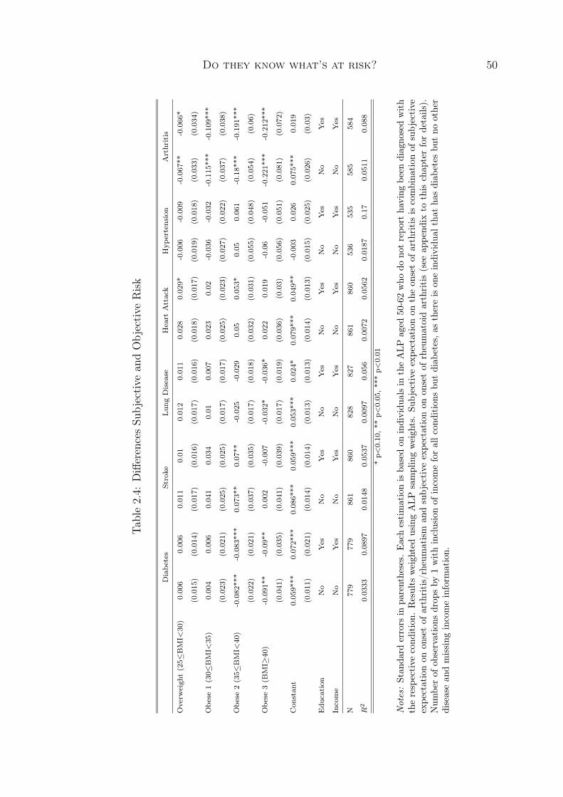
Do they know what’s at risk? 50
Table2.4:
DifferencesSu
bjective
andObjective
Risk
Diabe
tes
Stroke
Lun
gDisease
Heart
Attack
Hyp
ertension
Arthritis
Overw
eigh
t(25≤
BMI<
30)
0.006
0.006
0.011
0.01
0.012
0.011
0.028
0.02
9*-0.006
-0.009
-0.067**
-0.066*
(0.015)
(0.014)
(0.017)
(0.016)
(0.017)
(0.016)
(0.018)
(0.017)
(0.019)
(0.018)
(0.033)
(0.034)
Obe
se1(30≤
BMI<
35)
0.004
0.006
0.041
0.034
0.01
0.007
0.023
0.02
-0.036
-0.032
-0.115***
-0.109**
*
(0.023)
(0.021)
(0.025)
(0.025)
(0.017)
(0.017)
(0.025)
(0.023)
(0.027)
(0.022)
(0.037)
(0.038)
Obe
se2(35≤
BMI<
40)
-0.082***
-0.083***
0.073**
0.07**
-0.025
-0.029
0.05
0.053*
0.05
0.061
-0.18***
-0.191***
(0.022)
(0.021)
(0.037)
(0.035)
(0.017)
(0.018)
(0.032)
(0.031)
(0.055)
(0.048)
(0.054)
(0.06)
Obe
se3(B
MI≥
40)
-0.091**
-0.09**
0.002
-0.007
-0.032*
-0.036*
0.022
0.019
-0.06
-0.051
-0.221**
*-0.212***
(0.041)
(0.035)
(0.041)
(0.039)
(0.017)
(0.019)
(0.036)
(0.03)
(0.056)
(0.051)
(0.081)
(0.072)
Con
stan
t0.059*
**0.072***
0.086***
0.059***
0.053***
0.024*
0.079***
0.049**
-0.003
0.026
0.075***
0.019
(0.011)
(0.021)
(0.014)
(0.014)
(0.013)
(0.013)
(0.014)
(0.013)
(0.015)
(0.025)
(0.026)
(0.03)
Edu
cation
No
Yes
No
Yes
No
Yes
No
Yes
No
Yes
No
Yes
Income
No
Yes
No
Yes
No
Yes
No
Yes
No
Yes
No
Yes
N779
779
861
860
828
827
861
860
536
535
585
584
R2
0.0333
0.0897
0.0148
0.0537
0.0097
0.056
0.0072
0.0562
0.0187
0.17
0.0511
0.088
*p<
0.10,**
p<0.05,***p<
0.01
Not
es:Stan
dard
errors
inpa
rentheses.
Eachestimationisba
sedon
individu
alsin
theALP
aged
50-62who
dono
trepo
rtha
ving
been
diagno
sedwith
therespective
cond
ition.
Results
weigh
tedusingALP
samplingweigh
ts.Su
bjective
expe
ctationon
theon
setof
arthritisiscombina
tion
ofsubjective
expe
ctationon
onsetof
arthritis/rheumatism
andsubjective
expe
ctationon
onsetof
rheumatoidarthritis(see
appe
ndix
tothis
chap
terfordetails).
Num
berof
observations
drop
sby
1withinclusionof
incomeforallc
ondition
sbu
tdiab
etes,a
sthereis
oneindividu
althat
hasdiab
etes
butno
other
diseasean
dmissing
incomeinform
ation.

Do they know what’s at risk? 51
As the objective risks of most diseases for the normal- and underweight and ofchronic lung disease, heart attack and stroke among the overweight and obese arerelatively small on average, the general pattern of overestimation is in line with otherresults in the literature according to which individuals tend to overestimate smallprobability events (Lichtenstein et al., 1978). As diabetes risk increases significantlyfor the higher BMI groups, this might also explain why obese individuals have onaverage more accurate assessments of their risks of diabetes than the normal- andunderweight.
Interestingly the results in table 2.4 suggest that obese individuals underestimateone health risk, namely the risk of developing arthritis or rheumatism in the next 5years. On average, individuals with a BMI between 35 and 40 underestimate the riskby 10 percentage points and individuals in the highest BMI group underestimate therisk by about 15 percentage points.
The coefficients in the second column for each disease in table 2.4 result fromestimation of equation (2.4) with information on an individual’s educational attainmentand on household income included in addition to indicators of BMI categories. Theresults are essentially unchanged. Neither differences in educational attainment nordifferences in income can thus explain the underestimation of arthritis risk among theobese.
2.6 Robustness Analyses
In this section, we present several robustness analyses. First, we use estimates basedon a later HRS wave to calculate the objective risks in the ALP. Second, we employprobit models instead of duration models to estimate the relationship between indi-vidual characteristics and disease onset in the HRS. Third, we report estimates usingthe relative difference between subjective and objective risk instead of the absolutedifference as dependent variable.
The upper panel of table 2.5 displays coefficients and standard errors after esti-mation of equation (2.4) where the objective risk measure is based on HRS 1998 andfollow-up instead of on the first HRS wave.6 In order to ensure comparability to themain analysis, only individuals aged 50-62 from the HRS 1998 are used to estimatemodel (2.1). Using a later cohort in the HRS as baseline helps us to investigate whether
6The latest available wave that allows 5 years follow-up is wave 6, elicited in 2002. When infor-mation from this wave and follow-up is used, results are qualitatively and quantitatively unchangedfrom the ones displayed in the upper panel of table 2.5.

Do they know what’s at risk? 52
Table 2.5: Robustness Analyses I
Diabetes Stroke Lung Disease Heart Attack Hypertension Arthritis
Objective Risk based on duration model with HRS 1998 and follow-up
Overweight (25≤BMI<30) -0.005 0.009 0.014 0.034* -0.049** -0.042
(0.015) (0.017) (0.017) (0.018) (0.02 ) (0.033)
Obese 1 (30≤BMI<35) -0.022 0.046* 0.01 0.033 -0.075*** -0.139***
(0.023) (0.025) (0.018) (0.024) (0.028) (0.037)
Obese 2 (35≤BMI<40) -0.134*** 0.059 -0.025 0.056* 0.008 -0.193***
(0.023) (0.037) (0.018) (0.033) (0.053) (0.054)
Obese 3 (BMI≥40) -0.128*** 0.007 -0.055*** 0.02 -0.062 -0.236***
(0.041) (0.041) (0.018) (0.036) (0.053) (0.083)
Constant 0.055*** 0.083*** 0.048*** 0.076*** -0.041*** 0.053**
(0.01) (0.014) (0.013) (0.014) (0.015) (0.026)
N 779 861 828 861 536 585
R2 0.0643 0.0136 0.018 0.0101 0.0326 0.0668
Objective Risk based on probit model with HRS 1992 and follow-up
Overweight (25≤BMI<30) -0.002 0.014 0.018 0.03 -0.035* -0.067**
(0.015) (0.017) (0.017) (0.018) (0.019) (0.033)
Obese 1 (30≤BMI<35) -0.028 0.04 0.007 0.015 -0.078*** -0.114***
(0.023) (0.025) (0.017) (0.025) (0.027) (0.037)
Obese 2 (35≤BMI<40) -0.128*** 0.078** -0.027 0.042 0.02 -0.221***
(0.027) (0.037) (0.018) (0.032) (0.055) (0.057)
Obese 3 (BMI≥40) -0.177*** 0.007 -0.014 0.029 -0.186*** -0.332***
(0.043) (0.041) (0.017) (0.036) (0.06) (0.084)
Constant 0.06*** 0.083*** 0.046*** 0.073*** -0.011 0.037
(0.011) (0.013) (0.013) (0.014) (0.015) (0.026)
N 779 861 828 861 536 585
R2 0.083 0.0151 0.0089 0.0067 0.0789 0.0899
* p<0.10, ** p<0.05, *** p<0.01
Notes: Standard errors in parentheses. Dependent variables are differences between individual sub-jective and objective risks. Each estimation is based on individuals in the ALP aged 50-62 without adiagnosis of the specific condition prior to the ALP interview. Results weighted to take into accountsample selection. Subjective expectation on the onset of arthritis is combination of subjective expec-tation on arthritis/rheumatism onset and subjective expectation of rheumatoid arthritis onset (seeappendix to this chapter for details).
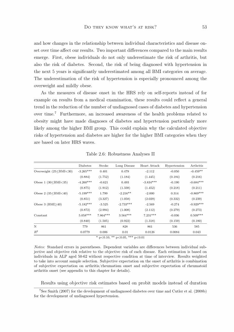
Do they know what’s at risk? 53
and how changes in the relationship between individual characteristics and disease on-set over time affect our results. Two important differences compared to the main resultsemerge. First, obese individuals do not only underestimate the risk of arthritis, butalso the risk of diabetes. Second, the risk of being diagnosed with hypertension inthe next 5 years is significantly underestimated among all BMI categories on average.The underestimation of the risk of hypertension is especially pronounced among theoverweight and mildly obese.
As the measures of disease onset in the HRS rely on self-reports instead of forexample on results from a medical examination, these results could reflect a generaltrend in the reduction of the number of undiagnosed cases of diabetes and hypertensionover time.7 Furthermore, an increased awareness of the health problems related toobesity might have made diagnoses of diabetes and hypertension particularly morelikely among the higher BMI group. This could explain why the calculated objectiverisks of hypertension and diabetes are higher for the higher BMI categories when theyare based on later HRS waves.
Table 2.6: Robustness Analyses II
Diabetes Stroke Lung Disease Heart Attack Hypertension Arthritis
Overweight (25≤BMI<30) -3.265*** 0.401 0.479 -2.112 -0.050 -0.459**
(0.884) (1.752) (1.184) (1.445) (0.184) (0.216)
Obese 1 (30≤BMI<35) -4.260*** -0.621 0.493 -3.834*** -0.190 -0.684***
(0.875) (1.912) (1.338) (1.452) (0.218) (0.211)
Obese 2 (35≤BMI<40) -5.199*** 1.799 -2.216** -2.000 0.314 -0.869***
(0.851) (3.327) (1.058) (2.029) (0.332) (0.239)
Obese 3 (BMI≥40) -5.182*** -3.525 -2.733*** -2.569 -0.274 -0.929***
(0.872) (2.994) (1.008) (2.112) (0.279) (0.273)
Constant 5.058*** 7.864*** 3.564*** 7.231*** -0.036 0.509***
(0.840) (1.505) (0.922) (1.318) (0.159) (0.180)
N 779 861 828 861 536 585
R2 0.0779 0.006 0.01 0.0126 0.0084 0.043
* p<0.10, ** p<0.05, *** p<0.01
Notes: Standard errors in parentheses. Dependent variables are differences between individual sub-jective and objective risk relative to the objective risk of each disease. Each estimation is based onindividuals in ALP aged 50-62 without respective condition at time of interview. Results weightedto take into account sample selection. Subjective expectation on the onset of arthritis is combinationof subjective expectation on arthritis/rheumatism onset and subjective expectation of rheumatoidarthritis onset (see appendix to this chapter for details).
Results using objective risk estimates based on probit models instead of duration7See Smith (2007) for the development of undiagnosed diabetes over time and Cutler et al. (2008b)
for the development of undiagnosed hypertension.

Do they know what’s at risk? 54
models are presented in the lower panel of table 2.5. Instead of the time to disease on-set as the dependent variable, we use an indicator variable that takes on the value oneif an individual is diagnosed with the specific condition sometime before the 4th waveof the HRS and is zero otherwise. The results confirm conclusions drawn in the mainanalysis. Obese individuals underestimate the risk of arthritis or rheumatism. More-over, there is evidence that the obese are overly optimistic about their risks of diabetesand hypertension, as they also underestimate the risks of the latter two diseases.
Table 2.6 reports results when the deviation of the subjective risk from the objectiverisk is measured relative to the objective risk. Instead of the difference in levels, we
use the difference relative to the objective risk, Sdi −OdiOdi
, as dependent variable in model
(2.4). The results are again similar to the results of the main analysis. Individualswho are normal- or underweight overestimate the risks of most diseases significantly.As the percent rather than percentage point metric puts an emphasis on deviationsfrom smaller objective values, it comes at no surprise that there are overestimationsbetween 350 and almost 800% for the diseases that show relatively low risks amongnormal- and underweight individuals. The risk of hypertension is not overestimatedand the risk of arthritis is overestimated by about 50% among the normal- and under-weight. Importantly, despite putting relatively less emphasis on deviations from higherobjective risks, we find evidence that individuals who are obese underestimate theirrisk of arthritis or rheumatism. Individuals with a BMI between 35 and 40 underesti-mate the risk by about 36% and individuals with a BMI over 40 underestimate theirrisk by 42%.
Overall, the robustness analyses confirm our main findings that obese individualsunderestimate the 5-year risk of arthritis or rheumatism. Furthermore, this sectionprovides evidence suggesting that also the risks of hypertension and diabetes are un-derestimated by individuals with excess body weight.
2.7 Conclusion
In this chapter, we add to the literature on risk perception among the overweight andobese by comparing subjective probabilities of developing different diseases within thefollowing 5 years to objective probabilities of the same events. Our results indicate thatindividuals who are normal- or underweight overestimate most disease risks. Similarly,the overweight tend to overestimate their risks. Obese individuals, however, under-estimate the risks of arthritis or rheumatism, diabetes and hypertension, while theyoverestimate the risks of heart attack and stroke.

Do they know what’s at risk? 55
These results are important for at least two reasons. First, diabetes and hyperten-sion are silent conditions that often do not show symptoms. Therefore they risk toremain undiagnosed. When undiagnosed the conditions cannot be treated adequatelyand are thus likely more harmful. Individuals who underestimate the risks of theseconditions might also be less likely to get checked for the conditions. The conditionsmight therefore remain undiagnosed longer, causing greater harm and higher medicalexpenses than if they were treated correctly.
Second, the results can provide guidance for designing health education programstargeted at the obese. While the medium term risks of cardiovascular disease, andin particular heart attack and stroke, is on average not underestimated by the obese,there is evidence that the risks of diabetes, hypertension and arthritis are not wellunderstood. Increasing the awareness of these risks among the obese might allow themto make better informed lifestyle choices and help them to opt for a more healthylifestyle.

Do they know what’s at risk? 56
Appendix
Results for smokers
In order to compare our results directly with the results of Khwaja et al. (2009), weestimate an equation similar to equation (2.4) where instead of the dummies for theBMI categories dummies for former and current smokers are included. Results aredisplayed in table 2.7. Despite some differences in the estimation method, the timehorizon and in the data used, our results support the findings by Khwaja et al. (2009).Neither current nor former smokers robustly underestimate any of the analyzed diseaserisks.
Subjective Expectations on Arthritis/Rheumatism
Subjective expectations on developing arthritis or rheumatism in the future are elicitedby two separate questions in the ALP. The first question asks individuals about theirchances of developing arthritis or rheumatism except rheumatoid arthritis, Pr(arthr),and the second question asks about the chances of developing rheumatoid arthritis,Pr(RA). In the HRS, however, there is only information on arthritis and rheumatismincluding rheumatoid arthritis. We therefore combine the answers to the two subjectiveexpectations question in the ALP.
As we are interested in whether overweight and obese individuals underestimatetheir risks of developing different diseases, we aggregate the two probabilities in a waythat results in the largest possible subjective probability of developing arthritis. Inparticular, we set
Pr(arthritis) = min{100;Pr(arthr) + Pr(RA)} (2.5)

Do they know what’s at risk? 57Ta
ble2.7:
Results
forSm
okers
Diabe
tes
Stroke
Lun
gDisease
Heart
Attack
Hyp
ertension
Arthritis
Objective
Riskba
sedon
HRS1992
Current
Smoker
-0.015
-0.012
-0.013
-0.015
0.022
0.026
-0.003
-0.009
-0.027
-0.00001
-0.014
-0.007
(0.02)
(0.021)
(0.02)
(0.02)
(0.021)
(0.02)
(0.021)
(0.02)
(0.023)
(0.022)
(0.04)
(0.042)
Form
erSm
oker
0.001
-0.003
0.011
0.003
0.012
0.006
0.004
-0.001
-0.003
-0.01
0.005
0.007
(0.016)
(0.016)
(0.019)
(0.018)
(0.013)
(0.012)
(0.018)
(0.017)
(0.021)
(0.02)
(0.032)
(0.032)
Con
stan
t0.056***
0.072***
0.104***
0.071***
0.048***
0.024***
0.099***
0.069***
-0.006
0.024
0.002
-0.038*
(0.011)
(0.017)
(0.011)
(0.012)
(0.007)
(0.008)
(0.011)
(0.012)
(0.013)
(0.022)
(0.019)
(0.023)
Edu
cation
No
Yes
No
Yes
No
Yes
No
Yes
No
Yes
No
Yes
Income
No
Yes
No
Yes
No
Yes
No
Yes
No
Yes
No
Yes
N779
779
861
860
828
827
861
860
536
535
585
584
R2
0.0016
0.0586
0.0023
0.0425
0.0042
0.0499
0.0002
0.049
0.0041
0.1537
0.0006
0.0424
Objective
Riskba
sedon
HRS1998
Current
Smoker
-0.007
-0.002
-0.018
-0.02
0.003
0.011
0.005
0.0004
-0.03
0.0005
-0.034
-0.018
(0.02)
(0.022)
(0.02)
(0.02)
(0.022)
(0.02)
(0.022)
(0.02)
(0.022)
(0.022)
(0.042)
(0.042)
Form
erSm
oker
0.008
0.005
0.011
0.004
0.009
0.005
0.008
0.004
-0.003
-0.007
0.002
0.011
(0.016)
(0.016)
(0.019)
(0.018)
(0.013)
(0.013)
(0.018)
(0.017)
(0.022)
(0.02)
(0.033)
(0.032)
Con
stan
t0.032***
0.051***
0.101***
0.068***
0.047***
0.031***
0.097***
0.06***
-0.068***
-0.024
-0.012
-0.037
(0.011)
(0.017)
(0.011)
(0.012)
(0.007)
(0.008)
(0.011)
(0.012)
(0.014)
(0.023)
(0.019)
(0.023)
Edu
cation
No
Yes
No
Yes
No
Yes
No
Yes
No
Yes
No
Yes
Income
No
Yes
No
Yes
No
Yes
No
Yes
No
Yes
No
Yes
N779
779
861
860
828
827
861
860
536
535
585
584
R2
0.0012
0.0583
0.0034
0.0431
0.0009
0.0473
0.0005
0.0482
0.0048
0.1678
0.0026
0.0548
*p<
0.10,*
*p<
0.05,*
**p<
0.01
Not
es:Stan
dard
errors
inpa
rentheses.
Eachestimationisba
sedon
individu
alsin
theALP
aged
50-62who
dono
trepo
rtha
ving
been
diagno
sedwith
therespective
cond
ition.
Results
weigh
tedusingALP
samplingweigh
ts.Su
bjective
expe
ctationon
theon
setof
arthritisiscombina
tion
ofsubjective
expe
ctationon
onsetof
arthritis/rheumatism
andsubjective
expe
ctationon
onsetof
rheumatoidarthritis(see
appe
ndix
tothis
chap
terfordetails).
Num
berof
observations
drop
sby
1withinclusionof
incomeforallc
ondition
sbu
tdiab
etes,a
sthereis
oneindividu
althat
hasdiab
etes
butno
other
diseasean
dmissing
incomeinform
ation.

Chapter 3
Heterogeneous Effects of Copayments:A Finite Mixture Bivariate ProbitAnalysis
3.1 Introduction
Analyses of reforms have traditionally focused on average effects. Average effects arehelpful, for example, in evaluating the cost-effectiveness of a reform. A comparison ofthe average returns generated by a reform to the average costs of the reform suffices todraw conclusions on cost-effectiveness. The average effect, however, might hide detailsthat are important for an overall evaluation of a reform. When the average effect ispositive, for example, but it is a combination of positive effects for most individuals andlarge negative effects for a few, this is likely of interest to the policy maker. Dependingon the policy maker’s objective function, the harm to the few might be more importantthan the gains for the many. It is therefore important to analyze whether a reformaffected different individuals differently.
In this paper, we develop and apply a finite mixture bivariate probit model thatallows to simultaneously analyze two types of effect heterogeneities. On the one hand,the finite mixture component of the model allows to estimate different reform effectsfor different latent classes of individuals. More specifically, it is assumed that there aredifferent classes or groups of individuals in the population, but that it is unobservedwhich individual belongs to which group. The observations within each group areassumed to be generated by the same distribution function. Between groups, however,any parameters of the distribution are allowed to vary. In the context of evaluatinga reform, the model allows for as many distinct reform effects as there are groups of

Heterogeneous Effects of Copayments 59
individuals; within each group individuals are assumed to be affected in the same way.On the other hand, the bivariate probit component of the model allows to jointly
estimate the effect on two distinct binary outcomes. The combination of the finitemixture and the bivariate probit component permits to study effects on the two binaryoutcomes within each of the latent classes at the same time. To our best knowledge,these two heterogeneities have up to now only been investigated under the assumptionof independence between the errors of the two outcome equations (Atella et al., 2004).In our model, this independence assumption is relaxed.
We apply the model to analyze heterogeneities in the effect of an increase of copay-ments for doctor visits and prescription drugs in the German statutory health insurancein 2004. The most radical element of the reform was an introduction of a per-quarterfee for doctor visits. Since 2004 patients have to pay e 10 for the first visit to a physi-cian in each quarter of the year. Further doctor visits to the same doctor within thequarter are free of charge for the patient. Visits in the same quarter to other doctorsare also exempt from the fee if the patient gets a referral by the doctor whom he visitedat first.
The literature that focuses on the effect of this specific reform delivers mixed results.Augurzky et al. (2006) and Schreyögg and Grabka (2010) find that the reform hadessentially no effect on the health care use of the statutorily insured in the GermanSocio-Economic Panel (SOEP). Using the same data set Farbmacher (2010), on thecontrary, presents evidence according to which the reform had an effect on the healthcare use of the statutorily insured. Farbmacher’s results are in line with Rückertet al. (2008) who find that individuals surveyed in the Bertelsmann Healthcare Monitorreport avoiding and delaying doctor visits due to the per-quarter fee. Our contributionsto this literature are twofold. We use a new data set to study the effect of the reform.In addition, our study is the first that analyzes whether this reform had heterogeneouseffects.
The data set that is employed in this analysis stems from insurance claims of thelargest German sickness fund. It includes information on doctor visits two years beforeand two years after the reform. An advantage of using insurance claims data is thatdoctor visits are reliably observed. We observe every doctor visit irrespective of whethera patient paid the per-quarter fee. Furthermore, the data includes information ondifferent types of doctor visits. In particular, it comprises information on visits togeneral practitioners (GPs) and on visits to specialists. This allows us to analyzewhether the reform had differential effects on these two types of doctor visits. Adisadvantage of the data is, however, that besides age and sex it does not contain any

Heterogeneous Effects of Copayments 60
socio-demographic information.Furthermore, the data set only includes few individuals who are exempt from the
copayments and could thus serve as a control group. We therefore apply a before-aftercomparison. Our results rely on the assumption that in the absence of the reformthere would not have been any changes in health care use. In the two years before andtwo years after the introduction of the copayments there were no other reforms in theGerman health care system.
In our analysis, we focus on the question whether the increase of the copaymentsin 2004 had an effect on the probability to visit a GP and/or a specialist at least oncewithin a year. We focus on the probability of visiting a doctor instead of on the numberof doctor visits within that period, because the reform should mainly affect access tohealth care. The e 10 fee only has to be paid for the first visit in a quarter. The pricefor additional doctor visits in the same quarter is therefore essentially zero.
Our results indicate that the average probability of at least one doctor visit, irre-spective of the doctor’s type, is 3 percentage points lower in the years after the reformthan in the years before the reform. The results are in line with Rückert et al. (2008)and Farbmacher (2010) and indicate that the reform affected the access to health care.
Furthermore, we find evidence for both of the analyzed heterogeneities. Whenallowing for two latent classes, the reform has a much stronger effect on individuals inone of the latent classes. The more affected class only comprises 24% of individuals.The two groups can be characterized by their probability of health care use prior tothe reform. The larger group has a probability of seeing at least one doctor per yearthat is almost 100%, we thus call them the likely users. The smaller group only goesto see a doctor with a probability of 66%. We call them the less-likely users. As thelikely users react less to the reform than the less-likely users our results are in line withfindings by Bago d’Uva (2006) and Winkelmann (2006) who present evidence that highusers of health care are less sensitive to increases in coinsurance and copayments thanlow users.
In addition, we find evidence that the two groups react differently for the two typesof doctor visits. Among the likely users the probability of seeing a GP is not affectedby the reform. The probability of seeing a specialist, however, decreases after thereform in this group. For the less-likely users, on the contrary, the probabilities ofboth types of doctor visits decline significantly after the reform. For a large group ofindividuals the introduction of the per-quarter fee might thus have strengthened theGP’s function as a gatekeeper in the health care system, even though the reform didnot force individuals to focus on GP visits only. Our results thus provide evidence that

Heterogeneous Effects of Copayments 61
it might be possible to strengthen the GP’s function as a gatekeeper without actuallylimiting individuals’ choices directly.
The chapter is structured as follows: Section 2 introduces our finite mixture bivari-ate probit model, the data used in the analysis is described in Section 3. Section 4presents the results, and Section 5 concludes.
3.2 Econometric Framework
Our data consists of a panel of individuals across time and across different physiciantypes. The patient can seek care from GPs (y1it) and/or specialists (y2it). The panel isunbalanced over time, and each individual i is observed in Ti periods. Over time andphysician types, individual i is thus observed 2 · Ti. Suppose that individual i belongsto a latent class j for the entire observational period. The probability of belonging toclass j is πj. Within a latent class, we use bivariate probits to jointly model the decisionto visit a GP and/or a specialist. The joint probability of the dependent variables overthe observed period is the product of Ti independent probabilities, given fixed classmembership, i.e.,
Pr(y1i, y2i|xi, θj) =
Ti∏t=1
Φ2[(2y1it − 1)xitβj, (2y2it − 1)xitγj, (2y1it − 1)(2y2it − 1)ρj](3.1)
where xi denotes the vector of covariates. θj contains the vector of parameters forGP visits (βj), for specialist visits (γj), and in addition the parameter ρj. The latterparameter indicates the extent to which the errors in the underlying structural modelcovary.The log-likelihood function is given by
ln(L) =I∑i=1
ln
(J∑j=1
πjPr(y1i, y2i|xi, θj)
)(3.2)
where I is the number of individuals in the dataset and J is the number of latentclasses. The likelihood function is maximized using the Newton-Raphson algorithm.First and second derivatives are calculated numerically in Stata’s optimization package.
Our finite mixture bivariate probit model is similar to the model developed byAtella et al. (2004). We expand their model by a panel dimension and thus use addi-tional information to determine class membership. While Atella et al. (2004) impose acorrelation of zero between the errors of the two outcome equations, we estimate these

Heterogeneous Effects of Copayments 62
correlations for each latent class. As the dependent variables are visits to differenttypes of physicians, the latter extension seems to be of particular importance.
For the interpretation of our results we calculate marginal effects on the marginaland joint outcome probabilities. Standard errors of the marginal effects are calculatedusing the delta method.1
3.3 Data
The analysis is based on insurance claims data from the largest German sickness fundin the years 2002 to 2005. The original data contains information on a 18.75% randomsubsample of all individuals in the German state of Hesse who are insured with thissickness fund.2 We only include individuals in our analysis who are at least 19 yearsold, as younger individuals are exempt from the copayments.3 Our sample is furtherrestricted to all individual-year pairs for which we observe the use of medical serviceswithin the entire year. Individual-year pairs, for example, in years within which anindividual switches from or to a different insurer or dies are excluded. This gives us thesame period at risk for each observation. Furthermore, in order to get a manageabledata set for our statistical analyses, we restrict the sample to a 3% random subsample.This gives us a sample with on average a little more than 7,000 individuals per year.
The data contains information on age and sex in addition to the information onhealth care use. Table 3.1 shows descriptive statistics for the different years. Theaverage age is almost unchanged over time. This reflects that we use an unbalancedpanel of individuals. The average number of doctor visits in our sample is almost 19per year. On average individuals visit a GP a little less than once a month and aspecialist around 7 times per year. This in international comparison relatively highuse of physician services is in line with information from other data on doctor visits inGermany. The average number of doctor visits in another large German wide sicknessfund, for example, is only slightly lower with 16.4 in 2004 and 16.9 in 2005 (Grobeet al., 2010).
While the average number of doctor visits per year does not change after the reform,at least one possible effect of the increased copayments becomes evident in table 3.1:Between 2003 and 2004, the fraction of individuals with at least one GP visit and the
1See appendix for details.2See http://www.pmvforschungsgruppe.de/content/02_forschung/02_b_sekundaerd_1.htm for a
short description of the data in German.3This feature of the reform suggests a natural devision in treatment and control group. We conduct
a difference-in-difference analysis for teenagers in a follow-up analysis.

Heterogeneous Effects of Copayments 63
Table 3.1: Descriptive Statistics
2002 2003 2004 2005Variable Mean SD Mean SD Mean SD Mean SDAge 52.35 18.55 52.47 18.66 52.58 18.64 52.49 18.72
19-39 0.30 0.46 0.29 0.45 0.28 0.45 0.28 0.4540-59 0.31 0.46 0.32 0.46 0.32 0.47 0.33 0.4760-79 0.32 0.47 0.32 0.47 0.32 0.47 0.31 0.46≥ 80 0.07 0.26 0.07 0.26 0.08 0.26 0.07 0.26
Female 0.52 0.50 0.52 0.50 0.52 0.50 0.52 0.50# GP visits 11.56 13.87 11.42 14.22 11.71 14.61 11.90 15.56GP>0 0.83 0.38 0.83 0.38 0.81 0.40 0.81 0.40# GP visits truncated at 0 13.95 14.10 13.84 14.54 14.52 14.96 14.76 16.06# Specialist visits 7.10 11.09 7.16 11.19 6.84 11.40 7.01 11.21Specialist>0 0.73 0.46 0.72 0.45 0.70 0.46 0.69 0.46# Specialist visits truncated at 0 9.77 11.97 9.89 12.09 9.75 12.53 10.1 12.24N 7,228 7,107 7,024 7,037
fraction with at least one specialist visit both decline by about 2 percentage points,from 83% to 81% for GPs and from 72% to 70% for specialists. Individuals thus seemto avoid to contact either type of doctor after the reform. There is also weak evidencethat the pattern of use might change after the reform. There are slightly more GP,and slightly less specialist visits in 2004 compared to 2003.
Figure 3.1: Development of GP and Specialist Visits Over Time

Heterogeneous Effects of Copayments 64
As the copayments can only be avoided by seeing neither type of physician, weare also interested in the different combinations of the outcome variables, i.e. whetheran individual visited both types of doctors at least once, or only one of the two, orneither. Figure 3.1 shows the development over time of the fractions of individualswho had different combination of doctor visits in the different years. While in 2002and 2003, roughly 10% of the sample visit neither a GP nor a specialist, this is thecase for about 12% of individuals in the years after the reform. The increase in thefraction of non-visitors is accompanied by small decreases in the other three fractions.
3.4 Results
In order to compare the results of the finite mixture bivariate probit model with resultsfrom models that just focus on average effects, and from models that analyze only oneof the two heterogeneities we estimate several models in addition to the one describedin section 3.2. In particular, we estimate a single equation probit model where thedependent variable combines the information on the two types of doctor visits to com-pare our results to others in the literature. We integrate a finite mixture componentwith two latent classes into this model to allow for different effects in different latentclasses.
Furthermore, differential effects on the two types of doctor visits are analyzed in abivariate probit model. This model is estimated imposing a correlation of 0 between theerror terms of the two underlying equations and relaxing this assumption. Similarly,when integrating the finite mixture component in the bivariate probit context, weestimate the model imposing a zero correlation and relaxing this assumption. We dothis in order to investigate whether our model improves upon the one presented byAtella et al. (2004).
3.4.1 Model Selection
Table 3.2 reports AIC and BIC information criteria for the different models. As thesingle equation probit models use a different dependent variable than the bivariateprobit models, the information criteria cannot be compared between the upper andthe lower part of the table. Within the lower and upper part, however, the informationin table 3.2 can help to select the model that fits the data best. In general, the tableindicates that models with two latent classes fit the data better than models that donot allow for unobserved heterogeneity. Restricting ρ to zero in the bivariate modelsleads to a deterioration of model fit in both, the degenerate and the finite mixture case.

Heterogeneous Effects of Copayments 65
Among the models in the lower part of table 3.2, the finite mixture bivariate probitmodel that allows for correlation between the error terms within each class shows thebest fit according to the AIC and BIC information criteria.
Table 3.2: Model Selection
Model N LogL df AIC BICProbit Visit 28,396 -9748.09 9 19514.18 19588.47FMM Probit Visit 28,396 -7729.19 19 15496.39 15653.21Bivariate Probit (ρ = 0) 28,396 -29567.2 18 59170.4 59318.97Bivariate Probit (ρ unrestricted) 28,396 -28076.14 19 56190.28 56347.1FMM Bivariate Probit (ρj = 0) 28,396 -24966.48 37 50006.96 50312.36FMM Bivariate Probit (ρj unrestricted) 28,396 -24887.91 39 49853.83 50175.74
Notes: Visit combines information on GP and specialists visits into one variable that is one if eithertype of doctor has been visited at least once.
3.4.2 Average Effects and one-way Heterogeneities
For means of comparison we begin with reporting the average marginal effects andstandard errors of the single equation probit models and the simple bivariate probitmodel with unrestricted ρ in table 3.3. The first two columns display average marginaleffects on the probability of at least one doctor visit per year, irrespective of thephysician type visited. The remainder of table 3.3 reports results with the two typesof heterogeneities introduced independently of each other. Columns 3 to 6 of table3.3 report results for two latent classes in the single equation probit. The averagemarginal effects and standard errors displayed in columns 7 and 8 are based on thebivariate probit model where the dependent variable is split to distinguish between theprobability to visit a GP and the probability to visit a specialist.
All estimations show significant changes in the probability of seeing a doctor afterthe increase of the copayments at the beginning of the year 2004. Marginal effectsreported in column 1 of table 3.3 indicate that the probability of at least one doctorvisit per year is 3 percentage points lower in 2004 and 2005 compared to 2002.
This overall effect hides heterogeneous reform effects in both analyzed dimensions.The finite mixture probit model reveals that individuals in the two latent classes reactdifferently to the reform. The estimate of the prior probability, π1, of belonging to latentclass 1 is 0.89%. In this larger fraction of the sample the probability of at least onedoctor visit only decreases by 1.9 percentage points in 2004 and 2.6 percentage points

Heterogeneous Effects of Copayments 66
Table 3.3: Marginal Effects after Probit, FMM Probit and Bivariate Probit
Probit FMM Probit Bivariate ProbitLatent Class 1 Latent Class 2
ME SE ME SE ME SE ME SEPr(Visit>0) Pr(Visit>0) Pr(Visit>0) Pr(GP>0)
Female 0.060*** 0.006 0.039*** 0.003 0.120*** 0.023 0.043*** 0.007Age Splines
Age 19-40 -0.001* 0.001 -0.001 0.0003 -0.001 0.002 0.0002 0.001Age 40-60 0.003*** 0.001 0.003*** 0.001 0.0004 0.004 0.004*** 0.001Age 60-80 0.001 0.001 0.0004 0.001 -0.0003 0.004 0.001 0.001Age > 80 -0.004 0.003 0.006 0.011 0.016** 0.008 -0.004 0.003
Year Dummies2003 -0.004 0.003 0.001 0.003 -0.032 0.027 -0.004 0.0042004 -0.032*** 0.004 -0.019*** 0.004 -0.138*** 0.027 -0.019*** 0.0052005 -0.034*** 0.004 -0.026*** 0.004 -0.099*** 0.028 -0.019*** 0.005
Pr(Specialist>0)Female 0.159*** 0.008Age Splines
Age 19-40 -0.001* 0.001Age 40-60 0.006*** 0.001Age 60-80 -0.006*** 0.001Age > 80 -0.011*** 0.003
Year Dummies2003 -0.003 0.0062004 -0.024*** 0.0062005 -0.030*** 0.006
ρ 0.572 0.011π1 0.887
* p<0.10, ** p<0.05, *** p<0.01
Notes: Marginal Effects on the probability stated at the top of each column. Visit combinesinformation on GP and specialists visits. π1 is the probability of class membership in latent class 1.Standard errors for the marginal effects are calculated using the delta method.
in 2005. In the other latent class the reaction amounts to 13.8 and 9.9 percentagepoint changes in the different years. There, thus, seems to be a rather small groupof individuals who reacted sharply to the reform while the rest only changed behaviormoderately.
The probabilities of different types of doctor visits are also affected differently bythe reform. The results in the last columns of table 3.3 show that the probability of

Heterogeneous Effects of Copayments 67
seeing a specialist at least once after the reform decreases more than the probabilityof seeing a GP. While the probability of seeing a GP at least once decreases by 1.9percentage points, the probability of seeing a specialist at least once is reduced by 2.4to 3 percentage points.
3.4.3 Simultaneous Evaluation of Heterogeneities
The finite mixture bivariate probit model allows to simultaneously analyze the twotypes of heterogeneities. Table 3.4 presents coefficients, average marginal effects, andstandard errors for the two dependent variables and the two latent classes. The es-timated prior probability of belonging to latent class 1, π1, is about 74%. There aredifferences in almost all parameter estimates between the two latent classes.
The sharpest difference between the two latent classes arises when focusing on thechanges over time. Probabilities in all other years are again compared to the year 2002as reference. In latent class 1 only the probability of at least one visit to a specialist in2005 decreases significantly compared to 2002, all other year parameter estimates arestatistically not different from 0. The increase of the copayments in 2004 did, thus,not affect the probability to see GPs and only had a delayed effect on the probabilityto see a specialist for this large fraction of the sample.
In latent class 2, on the contrary, the increase in the copayments in 2004 haschanged the probability of use of both types of physicians considerably. While in 2003,individuals are as likely to visit a GP at least once as in 2002, they are 8 percentagepoints less likely to visit a GP in 2004. In 2005, they are still 5.5 percentage pointsless likely to visit a GP compared to 2002. Similarly, the probability of at least onespecialist visit is reduced by 8 percentage points in 2004 and by 6 percentage pointsin 2005 compared to 2002. Combining the two types of heterogeneities in one modelthus allows the conclusion that a large group of individuals mainly reacted throughchanging their probability of seeing specialists, whereas among individuals in latentclass 2 the probability of both types of visits decreased significantly.
As the copayments can only be avoided entirely by not seeing any doctor, theeffect of the reform on the joint probability of neither seeing a GP nor a specialist isof particular interest. Table 3.5 reports average marginal effects on the different jointprobabilities for the three years 2003, 2004, and 2005 compared to 2002. Column 1 and2 of table 3.5 display the effects and their standard errors for latent class 1, columns 3and 4 for latent class 2, and the last two columns display the overall effect as a weightedaverage of the marginal effects in the two latent classes where the weight for each classis the probability of being in that class.

Heterogeneous Effects of Copayments 68
Table 3.4: FMM Bivariate Probit – Coefficients and Marginal Effects
Latent Class 1 Latent Class 2Coef SE ME SE Coef SE ME SE
GPFemale 0.002 0.041 0.0002 0.004 0.342*** 0.046 -0.256*** 0.015Age Splines
Age 19-40 0.011*** 0.003 0.001*** 0.0003 -0.004 0.005 -0.002 0.002Age 40-60 0.018*** 0.006 0.002*** 0.001 0.015* 0.008 0.005* 0.003Age 60-80 0.018 0.011 0.002 0.001 0.023*** 0.008 0.008*** 0.003Age > 80 -0.114* 0.062 -0.011* 0.006 -0.009 0.020 -0.003 0.007
Year Dummies2003 0.070 0.049 0.006 0.004 -0.071 0.045 -0.026 0.0172004 -0.008 0.050 -0.001 0.005 -0.214*** 0.047 -0.079*** 0.0172005 -0.080 0.049 -0.008 0.005 -0.149*** 0.047 -0.055*** 0.018
Constant 1.129*** 0.061 -0.421*** 0.094SpecialistFemale 0.748*** 0.031 0.551*** 0.008 0.286*** 0.041 0.103*** 0.015Age Splines
Age 19-40 -0.004 0.003 -0.001 0.001 0.003 0.005 0.001 0.002Age 40-60 0.027*** 0.005 0.006*** 0.001 0.000 0.007 0.0001 0.003Age 60-80 -0.021*** 0.006 -0.005*** 0.001 -0.004 0.007 -0.001 0.002Age > 80 -0.041*** 0.012 -0.009*** 0.003 -0.032 0.024 -0.012 0.009
Year Dummies2003 0.036 0.033 0.008 0.007 -0.077* 0.046 -0.029* 0.0172004 -0.025 0.033 -0.005 0.007 -0.222*** 0.048 -0.08*** 0.0172005 -0.092*** 0.033 -0.021*** 0.007 -0.172*** 0.048 -0.063*** 0.017
Constant 0.544*** 0.052 -0.539*** 0.090ρ 0.324*** 0.026 0.069*** 0.025π1 0.736
* p<0.10, ** p<0.05, *** p<0.01
Notes: π1 is the probability of class membership in latent class 1. Standard errors for the marginaleffects are calculated using the delta method.
The strongest reaction to the increase in copayments is again observed in latentclass 2. The probability of no doctor visit within a year increases by 9.5 percentagepoints in 2004 compared to 2002 while the probability to visit both types of physicians,a specialist and a GP, at least once within the year, decreases by 6.3 percentage points.In 2005, the effects are slightly smaller, but still highly significant. In latent class 1,on the contrary, the marginal probabilities do not change significantly in 2004. In
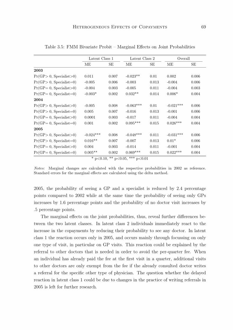
Heterogeneous Effects of Copayments 69
Table 3.5: FMM Bivariate Probit – Marginal Effects on Joint Probabilities
Latent Class 1 Latent Class 2 OverallME SE ME SE ME SE
2003Pr(GP> 0, Specialist>0) 0.011 0.007 -0.023** 0.01 0.002 0.006Pr(GP> 0, Specialist=0) -0.005 0.006 -0.003 0.013 -0.004 0.006Pr(GP= 0, Specialist>0) -0.004 0.003 -0.005 0.011 -0.004 0.003Pr(GP= 0, Specialist=0) -0.003* 0.002 0.032** 0.014 0.006* 0.0042004Pr(GP> 0, Specialist>0) -0.005 0.008 -0.063*** 0.01 -0.021*** 0.006Pr(GP> 0, Specialist=0) 0.005 0.007 -0.016 0.013 -0.001 0.006Pr(GP= 0, Specialist>0) 0.0001 0.003 -0.017 0.011 -0.004 0.004Pr(GP= 0, Specialist=0) 0.001 0.002 0.095*** 0.015 0.026*** 0.0042005Pr(GP> 0, Specialist>0) -0.024*** 0.008 -0.048*** 0.011 -0.031*** 0.006Pr(GP> 0, Specialist=0) 0.016** 0.007 -0.007 0.013 0.01* 0.006Pr(GP= 0, Specialist>0) 0.004 0.003 -0.014 0.011 -0.001 0.004Pr(GP= 0, Specialist=0) 0.005** 0.002 0.069*** 0.015 0.022*** 0.004
* p<0.10, ** p<0.05, *** p<0.01
Notes: Marginal changes are calculated with the respective probabilities in 2002 as reference.Standard errors for the marginal effects are calculated using the delta method.
2005, the probability of seeing a GP and a specialist is reduced by 2.4 percentagepoints compared to 2002 while at the same time the probability of seeing only GPsincreases by 1.6 percentage points and the probability of no doctor visit increases by.5 percentage points.
The marginal effects on the joint probabilities, thus, reveal further differences be-tween the two latent classes. In latent class 2 individuals immediately react to theincrease in the copayments by reducing their probability to see any doctor. In latentclass 1 the reaction occurs only in 2005, and occurs mainly through focussing on onlyone type of visit, in particular on GP visits. This reaction could be explained by thereferral to other doctors that is needed in order to avoid the per-quarter fee. Whenan individual has already paid the fee at the first visit in a quarter, additional visitsto other doctors are only exempt from the fee if the already consulted doctor writesa referral for the specific other type of physician. The question whether the delayedreaction in latent class 1 could be due to changes in the practice of writing referrals in2005 is left for further research.

Heterogeneous Effects of Copayments 70
Figure 3.2: Predicted Probabilities in 2002
The results suggest that the introduction of the per-quarter fee might have strength-ened the role of the GP in the German statutory health insurance. While GPs are notofficially implemented as gatekeepers, i.e. individuals can choose to directly visit aspecialist for a given disease and this would not cost them more than visiting a GPfirst, the reform nevertheless induces a large part of the sample to focus on GP visits.This might highlight the possibility of introducing gatekeeping into a health insurancesystem in a way that does not limit the patients’ choices.
Naturally, the question arises who the individuals are that belong to the differentlatent classes. Based on our model’s predictions, we can compare the two latent classesin terms of the probability of use of doctor visits. Figure 3.2 displays the predictedprobabilities of using the different types of physicians in 2002. It shows that in latentclass 1 the probability of no doctor visit within the year 2002 is about 2 percent. Mostof these individuals thus go to a doctor at least once within a year. And most ofthem see both, a GP and a specialist at least once. The probability to see both typesof physicians is 81 percent. In latent class 2, the picture looks very different. Thepredicted probability to see no physician at all within the year 2002 is 34 percent, theprobability to see both types of physicians is only 19 percent. Latent class 1 mightthus be described as the group of likely users, while individuals in latent class 2 are

Heterogeneous Effects of Copayments 71
the less-likely users.Overall, we find evidence for heterogeneous effects of increases in copayments.
When analyzing the two types of heterogeneities independently of each other, we findthat a large class of likely users of health care reacts much less to the increase in co-payments than the small class of less-likely users. Furthermore, the probability of atleast one visit to a GP decreases less than the probability of at least one visit to a spe-cialist. Simultaneously analyzing both types of heterogeneities reveals that the likelyusers not only react less strongly to the increase in copayments, but also by changingtheir pattern of use. While the less-likely users visit either type of physician with asmaller probability after the reform, likely users focus on one type of visit: Instead ofseeing GPs and specialists in a year, they only tend to visit GPs.
3.5 Conclusion
The interest in heterogeneous reform effects has recently increased in the literature.In order to evaluate heterogeneous effects, more sophisticated econometric models areneeded. In this chapter we develop and apply a finite mixture bivariate probit modelthat allows to estimate effects on two binary outcomes in different latent groups in thepopulation.
We apply our model to estimate the effects of an increase in copayments in theGerman statutory health insurance in 2004. In particular, we analyze whether thereform affected access to different types of health care differently in two latent groups.The different types of access to health care are measured as the probabilities of at leastone visit to a GP and of at least one visit to a specialist within a year. As earlierstudies of this reform did not distinguish between different types of doctor visits, wealso present results on general access to health care, measured as the probability of atleast one doctor visit per year, irrespective of the type of doctor visited. Furthermore,we gauge the contribution of our model by also analyzing the effects on the two typesof doctor visits without distinguishing between latent classes.
Using insurance claims data from the largest German sickness fund, we find thatthe probability to visit any kind of doctor at least once within a year decreases byabout 3 percentage points after the increase in the copayments. Distinguishing theresults between GP and specialist visits shows that the probability of at least one GPvisit decreases less than the probability of at least one specialist visit. Furthermore,we can distinguish two underlying groups: likely users who react less to the increasein copayments and less-likely users who show a strong reduction in the probability

Heterogeneous Effects of Copayments 72
to visit a doctor. This result aligns with findings in the literature that the demandfor health care is more elastic among low users of health care than among high users(Bago d’Uva, 2006; Winkelmann, 2006).
Combining the analysis of the two types of heterogeneities into one model allows touncover that the likely users not only react less to the increase in copayments than theless-likely users. They also react in a different way: While the less-likely users tend togo to neither type of doctor after the reform, the likely users change their behavior byfocussing on one type of doctor visits. They are more likely to visit only a GP after theincrease of the copayments and less likely to see both, a specialist and a GP. This mightindicate that per-quarter fees for doctor visits have the potential to concentrate visitsto one type of doctor. In particular, they may help to establish GPs as gatekeeperswithout actually forcing individuals to visit a GP first.

Heterogeneous Effects of Copayments 73
Appendix: Marginal Effects
Marginal effects on the probabilities of each type of doctor visit and on the joint prob-abilities for the different combinations of the different types of visits are calculated.Standard errors for the marginal effects are derived using the delta method. For con-tinuous explanatory variables the marginal effects are calculated using the calculusmethod. Marginal effects of binary variables are calculated with the finite differencemethod.
For a continuous variable x the marginal effect on the different joint probabilitiesfor y1i and y2i in latent class j are calculated for individual i
MExiPr(y1i, y2i|xi)j =∂Φ2(q1ix
′βj, q2ix′iγj, q1iq2iρj)
∂xi(3.3)
= q1iβx,jφ(q1ix′iβj)Φ
q2ix′iγj − q2
1iq2iρjx′iβj√
1− ρ2j
+ q2iγx,jφ(q2ix
′iγj)Φ
q1ix′iβj − q1iq
22iρjx
′iγj√
1− ρ2j
where Φ2 stands for the cumulative bivariate normal distribution function, Φ and
φ are the univariate standard normal cumulative distribution function and densityrespectively, and qki = 2yki − 1, where k ∈ {1, 2}. The values are averaged over allindividuals to get the average marginal effect.
Marginal effects of the continuous variable x on the marginal probabilities of theoutcomes in latent class j for individual i are calculated as
MExiPr(y1i = 1|xi)j = βx,jφ(x′iβj) (3.4)
MExiPr(y2i = 1|xi)j = γx,jφ(x′iγj) (3.5)
The individual marginal effects on the joint outcome probabilities of the years 2003,2004 and 2005 compared to 2002 in latent class j for individual i are calculated as
MEyear,iPr(y1i, y2i|xi)j = Φ2 (q1i(x′iβj + βyear,j), q2i(x
′iγj + γyear,j), q1iq2iρj) (3.6)
− Φ2(q1ix′iβj, q2ix
′iγj, q1iq2iρj)
where qki is defined as above, and βj and γj are vectors of parameter estimates forall variables but the year indicators. Again the averages of these marginal effects over

Heterogeneous Effects of Copayments 74
all individuals are reported.Marginal effects of the year dummies on the marginal probabilities for each indi-
vidual i are derived as
MEyear,iPr(y1i = 1|xi)j = Φ(q1i(x′iβj + βyear,j))− Φ(q1ix
′iβj) (3.7)
MEyear,iPr(y2i = 1|xi)j = Φ(q2i(x′iγj + γyear,j))− Φ(q2ix
′iγj) (3.8)
The overall marginal effect, i.e. the marginal effect averaged over the latent classes,for any continuous or discrete variable x is then derived as weighted average of themarginal effects across the different latent classes
MExi =∑j
πjMExi,j (3.9)
Averages over all individuals are reported.Standard errors for the average marginal effects are derived using the delta method
that delivers the variance for each average marginal effect as
V ar(ME) = ∇′gV ar(θ)∇g (3.10)
where θ is the vector of all parameters that are estimated (βj,γj,ρj, and p, whereπ = exp(p)
1+exp(p)) and ∇g stands for the gradient of the marginal effect, ME = g(θ), with
respect to θ. In order to calculate the variance on the average marginal effect, we seteach element in the gradient to its sample average.

Chapter 4
Is traditional teaching really all thatbad? A within-studentbetween-subject approach
4.1 Introduction
Recent studies stress the importance of teachers for student learning. However, thequestion what actually determines teacher quality, i.e. what makes one teacher moresuccessful in enhancing her students’ performance than another, has not been settled sofar (Aaronson et al., 2007). Different categories of teacher variables have been analyzed.Some studies focus on the impact of a teacher’s gender and race on teacher quality(Dee, 2005, 2007). Others try to uncover the relationship between student outcomesand teacher qualifications such as teaching certificates, other paper qualifications orteaching experience (Kane et al., 2008). Such observable teacher characteristics are,however, generally found to have only little impact on student achievement and canonly explain a relatively small part of overall teacher quality (Aaronson et al., 2007;Rivkin et al., 2005). Most of the variation in teacher quality can be attributed tounobserved factors.1
While most of these studies focus on characteristics of the teacher, this chapterdirectly peers into the black box of educational production by focusing on the actualteaching process. More specifically, we contrast two teaching practices (as currentlyimplemented in practice), teaching by giving lecture style presentations with teachingbased on in-class problem solving, and investigate the impact on student achievement.
1This finding led researchers, concerned with providing recommendations for recruitment policiesand designing optimal teacher pay schemes, to suggest to identify effective teachers by their actualperformance on the job using “value added” measures of student achievement (Gordon et al., 2006).

Is traditional teaching really all that bad? 76
Giving lecture style presentations is often regarded as old-fashioned and connected withmany disadvantages: Lectures fail to provide instructors with feedback about studentlearning and rest on the presumption that all students learn at the same pace. More-over, students’ attention wanes quickly during lectures and information tends to beforgotten quickly when students are passive. Finally, lectures emphasize learning bylistening, which is a disadvantage for students who prefer other learning styles. Alterna-tive instructional practices based on active and problem-oriented learning presumablydo not suffer from these disadvantages. National standards (NCTM, 1991; NationalResearch Council, 1996) consequently advocate engaging students more in hands-onlearning activities and group work. Despite these recommendations traditional lectureand textbook methodologies continue to dominate science and mathematics instructionin US middle schools (Weiss, 1997). This raises the question whether student achieve-ment could be raised by reducing the high share of teaching time devoted to lecturestyle presentations.
By addressing this question, this study adds to the literature analyzing the impactof teaching process variables such as teaching practices on student outcomes.2 Despitethe importance of teaching practices for student performance as recognized by educa-tional researchers (Seidel and Shavelson, 2007) and their potential relatively low-costimplementation, economists have only recently begun to analyze the impact of teach-ing methods on student achievement.3 Various dimensions of teaching practices havebeen shown to be able to explain a large share of the between-teacher variation in stu-dent achievement (Schacter and Thum, 2004). However, to our knowledge no rigorousempirical analysis of the effect of lecture style teaching compared to in-class problemsolving as implemented in practice today exists.4
To study the effect of lecture style teaching relative to teaching based on in-classproblem solving we use information on in-class time use provided by teachers in the2003 wave of the Trends in International Mathematics and Science Study (TIMSS) inUS schools. Estimating a reduced form educational production function and exploit-ing between-subject variation to control for unobserved student traits, we find thatthe choice of teaching practices matters for student achievement. We find that a 10
2For an overview see Goe (2007).3Brewer and Goldhaber (1997) and Aslam and Kingdon (2007) analyze the impact of many different
teaching methods. Rouse and Krueger (2004), Banerjee et al. (2007), and Barrow et al. (2009)investigate the effectiveness of computer-aided instruction and Machin and McNally (2008) analyzean education policy that changed reading instruction.
4Note that our results do not allow any comparison between teaching practices when implementedideally, but only allow a comparison of lecture-style teaching with problem-style learning approachesas implemented in practice.

Is traditional teaching really all that bad? 77
percentage point shift from problem solving to lecture style presentation results in anincrease in student achievement of about 1 percent of a standard deviation.
This result is highly robust. Consistent with other studies in this literature, wefind no evidence for significant effects of commonly investigated observable teachercharacteristics such as teaching certificates or teaching experience. While we are ableto control for a huge array of observable teacher traits, selection of teachers based onunobservable characteristics into teaching methods remains an issue. The bias resultingfrom potential selection of teachers with different unobservable attributes into differentteaching methods is assessed following the technique pioneered in Altonji et al. (2005).The results indicate that only relatively low selection on unobservables compared to theselection on observables is necessary to explain the entire estimated effect. We wouldthus not formulate policy conclusions that call for more lecture style teaching comparedto problem solving in general. However, a negative causal effect of giving lecture stylepresentations that is hidden in our results due to selection based on unobserved teachertraits is also not very likely. It can only exist if “good” teachers (teachers with favorableunobserved characteristics) predominately select themselves into an inferior teachingtechnique. This scenario, however, lacks any intuitive or theoretical support and thusappears extremely implausible. We therefore do not find any evidence that the highshare of total teaching time devoted to traditional lecture style teaching in scienceand mathematics instruction in US middle schools has detrimental effects on studentachievement. Our findings imply that simply changing the teaching method fromlecture style presentation to problem solving without concern for how the methods areimplemented has little potential for raising overall achievement levels.
The remainder of the chapter is structured as follows: the following section reviewsthe literature on teaching practices. Section 3 presents the data. Section 4 describesthe estimation strategy. Headline results are presented in Section 5, while Section 6provides a sensitivity analysis. Section 7 concludes.
4.2 Literature on Teaching Practices
There are two strands of literature that are closely related to our study. The first strandanalyzes the impact of different teaching styles on student achievement. In these studiesteaching style variables are meant to proxy for broader pedagogical concepts. A certainteaching style may consist of a combination of different teaching practices, where theterm teaching practice indicates the actual classroom activity, like giving a lecturestyle presentation or reviewing homework. The effects of single teaching practices are

Is traditional teaching really all that bad? 78
analyzed by the second strand of the related literature.Findings of the first strand of literature on teaching style speak in favor of mod-
ern, interactive teaching styles. Slavin et al. (2009) review recent research on theachievement outcomes of mathematics programs for middle and high schools. Themost striking observation of this review is the evidence supporting instructional processstrategies, especially cooperative learning. Several studies reveal important impacts ofcooperative learning programs that target teachers’ instructional behaviors rather thanmath content alone. The review concludes that educators and researchers might dowell to focus more on what is actually happening in the classroom.
In an earlier meta-analysis, Lou et al. (1996) focus on a typical component ofcooperative learning strategies, namely within-class grouping. The authors concludethat within-class grouping has the potential to raise student achievement. In particular,it works best when the physical placement of students into groups is combined withthe adaptation of instruction methods and materials for small-group learning. Dignathand Büttner (2008) find negative impacts of group work for primary school studentsin another meta-analysis. While these results are somehow in contradiction to thefindings by Lou et al. (1996) and Slavin et al. (2009), the authors emphasize thatpresumably the implementation of cooperative learning strategies into real classroomsettings matters.
Results from a study by Machin and McNally (2008) also support the idea thatcoordinated and comprehensive changes in instructional practices are beneficial forstudent learning. This study analyzes the effects of the introduction of the “literacyhour” in English primary schools in the late 1990s. This policy intervention by theBritish government changed how primary school students are taught to read. Usingthe fact that not all schools started the literacy hour at the same point in time in adifference-in-difference framework, the authors show that the literacy hour significantlyincreased reading skills for low ability student while high ability students were notaffected.
The findings of these studies suggest that the overall teaching style matters for stu-dent achievement. In particular, modern, interactive teaching styles have the potentialto positively affect student learning. However, the implementation of more interactiveteaching strategies into real classroom settings matters. There appear to be impor-tant interaction effects between individual instruction practices, curricula, teachingmaterials, and teacher experience with more interactive teaching styles.
The second strand of literature analyzes individual teaching practices more specifi-cally. A first group of studies in this area analyzes the use of computer based instruc-

Is traditional teaching really all that bad? 79
tion. The evidence on the use of computer programs is mixed for different subjects.On the one hand, Rouse and Krueger (2004) find that literacy skills of 3rd and 6thgrade students in a large US urban school district do not profit from the use of com-puter programs for teaching language and reading. Students’ math skills, on the otherhand, are found to increase due to computer-aided instruction as shown by Banerjeeet al. (2007) for India and Barrow et al. (2009) for the US. Computer-based instructionmight thus be more effective in some than in other subjects.
Other teaching practices that have received some attention in the literature areaccountability measures. Wenglinsky (2002) finds that frequent testing of studentsis positively related to students’ test scores taking into account student backgroundand prior performance. Bonesrønning (2004) analyzes if grading practices affect stu-dent achievement in Norway and finds evidence that easy grading deteriorates studentachievement. The design of tests might also matter. This hypothesis is supportedby findings of Matsumura et al. (2002). This study finds evidence for a positive linkbetween the quality of assignments that students are asked to do and overall studentperformance. These findings emphasize the importance of taking into account othercategories of in-class time use such as accountability measures when studying the ef-fect of teaching by giving lecture style presentations in comparison to in-class problemsolving.
More closely related to this chapter in terms of the teaching practices analyzed andidentification strategy are the analyses by Brewer and Goldhaber (1997) and Aslamand Kingdon (2007). Brewer and Goldhaber (1997) estimate different specifications ofeducation production functions for tenth grade students in math with data from theNational Educational Longitudinal Study of 1988. They conclude that teacher behavioris important in explaining student test scores. Controlling for student background,prior performance and school and teacher characteristics, they find that instruction insmall groups and emphasis on problem solving lead to lower student test scores.
Aslam and Kingdon (2007) analyze the impact of different teaching practices onstudent achievement in Pakistan. Their identification strategy rests on within studentacross subject (rather than across time) variation, which is similar to the identificationstrategy employed in this analysis. They find that students taught by teachers whospend more time on lesson planning and by teachers who ask more questions in classhave higher test scores.
Similar to this second strand of studies we focus on a comparison of single teachingpractices, namely time devoted to teaching by giving lecture style presentations versustime devoted to teaching by problem solving. As lecture style teaching is a teaching

Is traditional teaching really all that bad? 80
practice that is often associated with more traditional, didactic or teacher-centeredteaching styles, while problem solving is connected to more modern, interactive orstudent-centered approaches to teaching, our results might be also of a more generalinterest. Strictly speaking, however, our data only allows to draw conclusions aboutactual classroom activities.
4.3 Data
The data used in this study is the 2003 wave of the Trends in International Mathematicsand Science Study (TIMSS). In this study we focus on country information for the US.In TIMSS, students in 4th grade and in 8th grade were tested in math and science.We limit our analysis to 8th grade students, because 4th grade students are typicallytaught by one teacher in all subjects.
We standardize the test scores for each subject to be mean 0 and standard deviation1. In addition to test scores in the two tested subjects, the TIMSS data providebackground information on student home and family. For the purpose of this analysisit is crucial that TIMSS allows linking students to teachers. Each student’s teachersin math and science are surveyed on their characteristics, qualifications and teachingpractices. Additionally, school principals provide information on school characteristics.
The key variable of interest in this chapter is derived from question 20 in theteacher questionnaires in the 2003 wave of TIMSS. Unfortunately, this precise questionwas not asked in previous waves of TIMSS. We therefore limit our analysis to the2003 wave. Teachers are asked in 2003 to report what percentage of time in a typicalweek of the specific subject’s lessons students spend on eight in-class activities. Ourthree main categories of interest are listening to lecture style presentation, workingon problems with the teacher’s guidance and working on problems without guidance.The overall time in class spent on these three activities likely provides a good proxyfor the time in class in which students are taught new material. The main interestof this study is to contrast teaching by giving lecture style presentations to teachingbased on problem solving. The two problem solving categories are thus combined intoa single teaching practice: teaching based on problem solving. To allow a comparisonof the two categories we construct a single variable, lecture style teaching, that is thepercent of time spent giving lecture style presentation relative to the percent of timespent on either of the two activities ( lecture(%)
lecture(%)+problemsolving(%)). The key advantage is
that a change in this variable can directly be interpreted as a shift from spending timeon one to spending time on the other practice holding constant the overall time spent

Is traditional teaching really all that bad? 81
on these two practices. For example, an increase in this variable of 0.1 indicates that10 percentage points of total time devoted to teaching new material are shifted fromteaching based on problem solving to giving lecture style presentations.
The remaining 5 activities include reviewing homework, listening to the teacherreteach and clarify content, taking tests or quizzes, classroom management and otheractivities. We simply group these activities and construct a single variable, other classactivities, which measures the share of total time in class spent on other activities.We include this variable as a control in all specifications. To analyze the robustnessof our results we also estimate specifications that include the individual shares of allcategories. Moreover, teachers also report the total time in minutes per week that theyteach math or science to the class, which we also include as a control variable in mostspecifications.
The TIMSS 2003 US data set contains student-teacher observations on 8,912 stu-dents in 232 schools. 41 of those students have more than one teacher in science. Thesestudents are not included in the estimation sample. 8,871 students in 231 schools in455 math classes taught by 375 different math teachers and in 1,085 science classestaught by 475 different science teachers remain in the sample. Not all of the studentsand teachers completed their questionnaires. In order not to lose a large amount ofobservations we impute missing values of all control variables and include indicators forimputed values in all estimations.5 2,561 students have, however, missing informationon our teaching practice variable of interest. These observation are dropped from theanalysis. 6,310 students in 205 schools with 639 teachers (303 math teachers and 355science teachers, where 19 teachers teach both subjects) remain in the sample.
Furthermore due to the sampling design of TIMSS, students are not all selectedwith the same probability. A two stage sampling design makes it necessary to takeprobability weights into account when estimating summary statistics (Martin, 2005).All estimation results take the probability weights into account and allow for correlationbetween error terms within schools.6
Table 4.1 reports descriptive statistics on observable teacher characteristics sepa-rately for math and science teachers. Mean differences are reported in the last columnof table 4.1. The share of teachers with math or science majors naturally differs be-
5Experimenting with different imputation procedures revealed that our main results do not dependon the method of imputation. Main results remain also qualitatively unchanged when simply deletingobservations with missing values. Results presented in the chapter are based on a simple mean-imputation procedure.
6In addition, the two step procedure of sampling could be incorporated in the estimation of standarderrors. For simplicity, we ignore the latter in the following analysis which then gives us conservativeestimates of the standard errors.

Is traditional teaching really all that bad? 82
Table 4.1: Descriptive Statistics – Teacher variables
Math Science303 teachers 355 teachers
Variable Mean SD Mean SD Difference
In-class time useLecture style teaching 0.320 0.187 0.374 0.202 -0.054***Other class activities 0.428 0.119 0.446 0.161 -0.018Total teaching time ( min
week) 226.27 43.89 223.72 47.34 2.55
Teacher variablesTeacher is female 0.649 0.473 0.540 0.496 0.109**Full teaching certificate 0.970 0.163 0.957 0.188 0.013Major in math 0.473 0.492 0.099 0.294 0.374***Major in science 0.146 0.348 0.584 0.486 -0.438***Major in education 0.598 0.483 0.456 0.491 0.142***Teacher younger than 30 0.119 0.322 0.143 0.349 -0.024Teacher aged 30-39 0.273 0.443 0.223 0.414 0.050Teacher aged 40-49 0.293 0.452 0.335 0.469 -0.042Teaching experience < 1 year 0.043 0.201 0.042 0.199 0.001Teaching experience 1-5 years 0.178 0.370 0.224 0.404 -0.046Teacher training 0 years 0.102 0.301 0.154 0.359 -0.051**Teacher training 1 year 0.578 0.491 0.523 0.497 0.055Teacher training 2 years 0.209 0.404 0.193 0.392 0.016Teacher training 3 years 0.039 0.192 0.048 0.213 -0.009Teacher training 4 years 0.056 0.228 0.035 0.184 0.021Teacher training 5 years 0.008 0.090 0.039 0.193 -0.031**
MotivationPedagogy classes in last 2 years 0.748 0.431 0.648 0.472 0.100***Subject content classes in last 2 years 0.840 0.364 0.827 0.374 0.014Subject curriculum classes in last 2 years 0.830 0.372 0.853 0.349 -0.023Subject related IT classes in last 2 years 0.729 0.441 0.803 0.393 -0.074**Subject assessment classes in last 2 years 0.756 0.426 0.649 0.471 0.107***Classes on improving student’s skills last 2 years 0.759 0.424 0.766 0.418 -0.007Working hours scheduled per week 21.12 8.28 20.16 7.29 0.960Weekly hours spent on lesson planning 3.70 2.71 4.68 3.28 -0.976***Weekly hours spent on grading 5.25 3.93 6.08 4.41 -0.830**
Teaching requirementsRequirement probationary period 0.502 0.493 0.496 0.479 0.007Requirement licensing exam 0.526 0.493 0.558 0.479 -0.032Requirement finished Isced5a 0.891 0.307 0.824 0.371 0.067**Requirement minimum education classes 0.833 0.368 0.777 0.399 0.056Requirement minimum subject specific classes 0.799 0.395 0.744 0.420 0.056
Note: Probability weights and within school correlation are taken into account when estimating meansand standard deviations. Teacher variables are weighted by the number of students taught by eachteacher.

Is traditional teaching really all that bad? 83
tween those two groups. Apart from mean differences in majors several other variablesare significantly different between the two groups. We control for all these observabledifferences in teacher traits in our empirical analysis.
To investigate which teachers teach using relatively more lecture style presentationsand which students are more exposed to this method tables 4.2 and 4.3 display averagesof student, school, class and teacher characteristics grouped by the share of lecturestyle presentation. The last column of tables 4.2 and 4.3 presents the mean differencesbetween characteristics of students, schools, classes and teachers with more and lessthan the median share of time spent on lecture style presentation.
Table 4.2 reveals that the only student characteristic which shows significant dif-ferences between the two groups is the number of books that families have at home.Students who are taught with relatively less time spent on lecture style presentationsseem to have fewer books at home. Furthermore, the share of students in schools forwhich the principal reports very low involvement of parents in school activities is higheramong students taught with relatively less time spent on lecture style presentations.Students exposed to smaller shares of class time devoted to lecture style teaching arealso slightly more likely to be in tracked classes.
Table 4.3 reports teacher characteristics by the intensity of lecture style teaching.Students taught with relatively less time spent on lecture style teaching have a highershare of female teachers, more teachers who are at least 50, teachers who have themaximum number of years of teacher training, and teachers who have taken pedagogicalor content knowledge classes in the last two years. All other teacher characteristics donot differ significantly between the two groups.
Tables 4.2 and 4.3 indicate some potential for selection into different teaching prac-tices. To control for the confounding impact of these differences in observable char-acteristics, we include all variables presented in the tables above and additional in-formation on teaching limits (see table 4.8 in the appendix) in our empirical analysis.The latter are teacher reports on limitations that they face in teaching. These includelimitations through the class composition, shortages in teaching material, and a highstudent teacher ratio.
4.4 Estimation Strategy
To estimate the effect of giving lecture style presentations relative to teaching basedon problem solving we estimate a standard education production function:

Is traditional teaching really all that bad? 84
Table 4.2: Student, School and Class Variables by Intensity of Lecture Style Teaching
Lecture Style Lecture Style> median <= median
Variable Mean SD Mean SD Difference
StudentAge 14.22 0.451 14.23 0.470 -0.014Born in first 6 months 0.501 0.499 0.495 0.499 0.005Girl 0.522 0.500 0.522 0.499 0.000Number books at home: 11-25 0.175 0.378 0.173 0.376 0.002Number books at home: 26-100 0.282 0.448 0.278 0.445 0.004Number books at home: 101-200 0.185 0.387 0.173 0.375 0.013*Number books at home: >200 0.248 0.430 0.250 0.430 -0.002Parental Education lower secondary 0.057 0.208 0.058 0.211 -0.001Parental Education upper secondary 0.248 0.388 0.253 0.392 -0.005Parental Education post secondary voc/technical 0.094 0.264 0.088 0.254 0.006Parental Education university 0.577 0.445 0.571 0.446 0.006Number people at home 3 0.165 0.368 0.170 0.372 -0.005Number people at home 4 0.347 0.472 0.350 0.472 -0.003Number people at home 5 0.255 0.432 0.251 0.429 0.004Number people at home 6 0.108 0.307 0.104 0.303 0.003Number people at home 7 0.046 0.207 0.042 0.198 0.004Number people at home 8 or more 0.039 0.192 0.039 0.193 0.000Never speaks English at home 0.044 0.205 0.048 0.213 -0.004Sometime speaks English at home 0.099 0.298 0.093 0.289 0.006Almost always speaks English at home 0.845 0.360 0.843 0.361 0.002Immigrant 0.141 0.347 0.144 0.349 -0.003
SchoolCommunity, 3001-15,000 people 0.188 0.375 0.228 0.403 -0.041Community, 15,001-50,000 people 0.330 0.454 0.293 0.435 0.037Community, 50,001 - 100,000 people 0.121 0.314 0.118 0.309 0.003Community, 100,001 - 500,000 people 0.137 0.331 0.130 0.321 0.007Community, more than 500,000 people 0.125 0.319 0.111 0.299 0.014Parental involvement in school - very low 0.130 0.319 0.204 0.384 -0.074**Parental involvement in school - low 0.389 0.469 0.324 0.442 0.065Parental involvement in school - medium 0.300 0.440 0.316 0.441 -0.016Parental involvement in school - high 0.118 0.311 0.101 0.285 0.017
Class variablesTotal teaching time ( min
week) 221.93 48.60 227.45 43.03 -5.52
Class size 23.95 6.90 24.03 7.20 -0.073Tracked according to ability 0.319 0.452 0.394 0.469 -0.075*
Note: Lecture style measures the share of teaching time devoted to lecture style teaching instead ofteaching based on problem solving. Median refers to the median of lecture style teaching. Probabilityweights and within school correlation are taken into account when estimating means and standarddeviations.

Is traditional teaching really all that bad? 85
Table 4.3: Teacher Variables by Intensity of Lecture Style Teaching
Lecture Style Lecture Style> median <= median
Variable Mean SD Mean SD Difference
Teacher variablesTeacher is female 0.535 0.496 0.642 0.475 -0.107**Full teaching certificate 0.947 0.216 0.977 0.135 -0.031Major in math 0.265 0.432 0.303 0.455 -0.039Major in science 0.385 0.477 0.349 0.471 0.036Major in education 0.515 0.490 0.537 0.493 -0.022Teacher younger than 30 0.127 0.331 0.134 0.339 -0.007Teacher aged 40-49 0.367 0.480 0.272 0.442 0.096**Teacher at least 50 0.256 0.434 0.347 0.473 -0.091**Teaching experience < 1 year 0.045 0.205 0.041 0.197 0.004Teaching experience 1-5 years 0.229 0.406 0.180 0.372 0.049Teacher training 0 years 0.130 0.334 0.127 0.331 0.003Teacher training 1 year 0.568 0.492 0.537 0.496 0.031Teacher training 2 years 0.213 0.407 0.191 0.391 0.022Teacher training 3 years 0.036 0.185 0.050 0.216 -0.013Teacher training 4 years 0.040 0.195 0.050 0.216 -0.009Teacher training 5 years 0.008 0.089 0.036 0.186 -0.028**
Teacher motivationPedagogy classes in last 2 years 0.633 0.476 0.749 0.429 -0.116***Subject content classes in last 2 years 0.792 0.402 0.865 0.338 -0.073**Subject curriculum classes in last 2 years 0.818 0.381 0.860 0.342 -0.042Subject related IT classes in last 2 years 0.780 0.409 0.754 0.427 0.025Subject assessment classes in last 2 years 0.671 0.464 0.728 0.441 -0.057Classes on improving student’s skills last 2 years 0.757 0.424 0.768 0.418 -0.011Working hours scheduled per week 20.82 7.45 20.50 8.09 0.322Weekly hours spent on lesson planning 4.29 3.14 4.12 2.96 0.170Weekly hours spent on grading 5.66 3.85 5.67 4.45 -0.013
Teaching requirementsRequirement probationary period 0.503 0.484 0.496 0.487 0.008Requirement licensing exam 0.523 0.486 0.556 0.487 -0.033Requirement finished ISCED 5a 0.858 0.340 0.857 0.343 0.001Requirement minimum education classes 0.779 0.402 0.826 0.369 -0.047Requirement minimum subject specific classes 0.740 0.425 0.797 0.392 -0.056
Note: Lecture style measures the share of teaching time devoted to lecture style teaching instead ofteaching based on problem solving. Median refers to the median of lecture style teaching. Probabilityweights and within school correlation are taken into account when estimating means and standarddeviations. Teacher variables are weighted by the number of students taught by each teacher.

Is traditional teaching really all that bad? 86
Yijk = cj +B′ijkβ1j + S ′ijkβ2j + T ′ijkβ3j + Lectureijkβ4j + εijk. (4.1)
The test score, Yijk, of student i in subject j in school k is explained by a subjectspecific constant cj, student background characteristics, Bijk, school characteristics,Sijk, teacher and class characteristics, Tijk, and the variable Lectureijk. The lastvariable constitutes the focus of this analysis. It represents teaching time spent onlecture style presentation relative to problem solving. The error term, εijk, contains allunobservable influences on student test scores. In particular, it contains the effects ofunobservable student, µi , teacher, ξj, and school characteristics, νk:
εijk = µi + ξj + νk + ψijk (4.2)
Estimating equation (4.1) by ordinary least squares produces biased estimates ifunobserved school characteristics, νk, and Lectureijk are correlated. This can be thecase if the choice of the teaching practice is partly determined by the school and ifthere exists sorting of high ability students or effective teachers into schools.
To eliminate the effects of between-school sorting, we use school fixed effects, sk, toexclude any systematic between-school variation in performance or teaching practice,whatever its source:
Yijk = cj +B′ikβ1j + sk + T ′ijkβ3j + Lectureijkβ4j + µi + ξj + ψijk. (4.3)
The estimates produced by equation (4.3) could still be biased by within-schoolsorting wherever schools have more than one class per subject per grade. We thereforeeliminate the influence on constant student traits by differencing between subjects:
∆Yi = cm − cs +B′i(β1m − β1s) + S ′i(β2m − β2s) (4.4)
+T ′imβ3m − T ′isβ3s + Lectureimβ4m − Lectureisβ4s + ηi
where ∆Yi = Yim − Yis and ηi = ξm − ξs + ψim − ψis.In our headline specification we follow Dee (2005, 2007) by assuming that coeffi-
cients for each variable are equal across the two subjects:7
∆Yi = ∆T ′iβ3 + ∆Lectureiβ4 + ηi. (4.5)7We do, however, estimate equation (4.4) as a robustness check.

Is traditional teaching really all that bad? 87
The estimate of the effect of teaching practice on student achievement producedby equation (4.5) is not biased due to between or within school sorting of studentsbased on unobservable student traits. We do, however, have to make the identifyingassumption that unobservable teacher characteristics that directly influence studentachievement are not related to the choice of the teaching method. In other words, ηi isuncorrelated with all other right-hand side variables. This is a strong assumption andwe therefore refrain from interpreting β4 as causal effect. We rather interpret β4 as ameasure for the link between a teaching practice and student achievement that is notdriven by between or within school sorting of students. It might, however, be partlydriven by sorting of teachers into a special teaching method based on unobservableteacher traits.
We evaluate the concern of selection on unobservables by borrowing a procedurefrom Altonji et al. (2005) which allows to evaluate the bias of the estimate under theassumption that selection on unobservables occurs to the same degree as selection onobservables. As developed in the appendix the asymptotic bias of β4 in our applicationis
Bias(β4) =Cov( ˜∆Lecture, η)
V ar( ˜∆Lecture)=Cov(∆Lecture, η)
V ar( ˜∆Lecture)(4.6)
where indices are omitted for simplicity and where ˜∆Lecture is the residual ofa linear projection of ∆Lecture on all other between-subject differences of controlvariables, represented by ∆T . The second equality holds if the other controls (T ) areorthogonal to η. The condition that selection on unobservables is equal to selection onobservables can be stated as
Cov(∆T ′β3,∆Lecture)
V ar(∆T ′β3)=Cov(∆Lecture, η)
V ar(η)(4.7)
Equation (4.7) can be used to estimate the numerator of the bias of β4, once we haveconsistent estimates for β3. Under the assumptions that the true effect of lecture styleteaching is zero and again that T is orthogonal to η, β3 can be consistently estimated(see appendix).
The estimated bias displays the effect we would estimate even if the true effectwas zero when selection on unobservables is as strong as selection on observables. Inaddition, we report the ratio of the estimated β4 from equation (4.5) and the estimated

Is traditional teaching really all that bad? 88
bias giving a hint of how large selection on unobservables would have to be comparedto selection on observables to explain the entire estimated effect. A value higher thanone indicates that selection on unobservables needs to be stronger than selection onobservables to explain the entire estimate, in case of a ratio lower than one alreadyweaker selection on unobservables than on observables suffices to explain the entireestimate.
4.5 Results
Estimates of the effect of teaching practices based on the different methods advancedin Section 4.4 are presented in Tables 4.4 and 4.5. Each regression is performed at thelevel of the individual student and each of the estimations also takes into account thecomplex data structure produced by the survey design and the multi-level nature ofthe explanatory variables.
Table 4.4 reports results from estimating equation (4.1) and equation (4.3). Weestimate both equations separately for math and science. Columns 1 and 3 presentregressions results for math and science based on equation (4.1). These regressionsinclude a complete set of student- and family-background variables, controls for teacherand class characteristics as well as characteristics of the school. Given the purpose ofthis study, only estimated coefficients for the teaching practice variable of interest andselected teacher characteristics are reported.
Our key variable of interest, teaching time devoted to lecture style presentationrelative to time spent on problem solving, is estimated to have a positive impact on testscores in both subjects. In math the estimate is highly significant, while the estimatein science falls short of achieving statistical significance at any common significancelevel.
As discussed in the previous section, these results might be confounded by betweenschool sorting based on unobservable characteristics of students. Column 2 and 4therefore report estimation results based on equation (4.3), which includes school fixedeffects. Lecture style presentation is now highly significant in science and the pointestimate significantly increased compared to column 3. The estimate in math, however,did not change, but lost its statistical significance due to increased standard errors.
To gain statistical power we pool both estimation samples and estimate equations(4.1) and (4.3) with the joint sample. This approach assumes that the effects of allright-hand side variables are identical in both subjects. Based on this estimation samplethe relationship between more lecture style presentation and test scores is positive and

Is traditional teaching really all that bad? 89Ta
ble4.4:
Estim
ationResults
OLS
Math
Math
Science
Science
Poo
led
Poo
led
Lecturestyleteaching
0.514**
0.431
0.207
0.690**
0.380***
0.293***
(0.205)
(0.396)
(0.132)
(0.292)
(0.111)
(0.088)
Other
classactivities
–0.070
–0.701
0.042
–0.461
0.022
–0.322**
(0.298)
(0.523)
(0.161)
(0.301)
(0.140)
(0.135)
Total
teaching
time(m
inweek∗
10−3)
0.004
0.328
–0.329
–0.157
–0.064
0.070
(0.657)
(2.977)
(0.559)
(0.873)
(0.412)
(0.454)
Femaleteacher
–0.156**
–0.171
–0.075
–0.022
–0.098**
–0.019
(0.065)
(0.120)
(0.056)
(0.096)
(0.047)
(0.038)
Teacher
youn
gerthan
300.125
0.074
0.116
0.256*
0.110
0.054
(0.136)
(0.237)
(0.093)
(0.143)
(0.079)
(0.079)
Teacher’s
age40-49
0.054
0.075
0.054
0.127
0.051
0.001
(0.079)
(0.179)
(0.075)
(0.104)
(0.051)
(0.046)
Teacher
olderthan
500.024
0.113
0.083
–0.023
0.034
0.016
(0.082)
(0.181)
(0.073)
(0.128)
(0.057)
(0.059)
Teachingexpe
rience<1years
–0.513***
–0.878***
–0.116
–0.022
–0.266**
–0.160*
(0.155)
(0.242)
(0.167)
(0.175)
(0.105)
(0.093)
Teachingexpe
rience
1-5years
–0.202**
–0.303*
–0.016
–0.032
–0.103
–0.077
(0.097)
(0.178)
(0.072)
(0.101)
(0.068)
(0.069)
Teachingcertificate
–0.368**
–1.229***
0.057
–0.358
–0.040
–0.132
(0.170)
(0.318)
(0.180)
(0.383)
(0.137)
(0.161)
Con
stan
t0.898
1.891
–0.015
2.340***
0.345
0.345
(0.546)
(1.298)
(0.563)
(0.725)
(0.492)
(0.423)
Stud
entba
ckgrou
ndYes
Yes
Yes
Yes
Yes
Yes
Scho
olvariab
les
Yes
No
Yes
No
Yes
No
Scho
olfix
edeff
ects
No
Yes
No
Yes
No
Yes
Teacher
variab
les
Yes
Yes
Yes
Yes
Yes
Yes
Class
variab
les
Yes
Yes
Yes
Yes
Yes
Yes
Observation
s6,310
6,310
6,310
6,310
12,620
12,620
R2
0.313
0.518
0.337
0.501
0.309
0.476
*p<
0.10,**
p<0.05,***p<
0.01
Not
e:Dep
endent
variab
leis
thestan
dardized
stud
enttest
score.
Lecturestylemeasurestheshareof
teaching
timedevo
tedto
lecturestyleteaching
insteadof
teaching
basedon
prob
lem
solving.
Stud
entba
ckgrou
ndinclud
esstud
ents’g
ender,
agein
years,
adu
mmyifbo
rnin
first
6mon
thsof
the
year,nu
mbe
rof
book
sat
home,
Eng
lishspoken
atho
me,
migration
backgrou
nd,ho
useholdsize
andpa
rental
education.
Scho
olvariab
lesinclud
edu
mmiescapturingdiffe
rent
levels
ofpa
rental
involvem
entin
scho
olactivities
anddu
mmiesforcommun
itysize.Not
repo
rted
teachervariab
lesare
teacher’smajor
inmath,
sciencean
deducationan
dyearsof
teachertraining
.Class
variab
lesareclasssize,an
datracking
indicator.
Impu
tation
indicators
areinclud
edin
allr
egressions.Stan
dard
errors
clusteredat
thescho
ollevelinpa
rentheses.

Is traditional teaching really all that bad? 90
significantly different from zero in both specifications.The evidence presented in table 4.4 suggests a positive relation between more lecture
style presentation and student achievement. However, within school selection of stu-dents based on unobservable student characteristics might drive this relationship. Forinstance, it is reasonable to assume that teachers adjust the use of teaching practicesaccording to class composition and average student ability. We therefore difference outunobserved constant student traits by taking between-subject differences of test scoresand all right-hand side variables as presented in equation (4.5).
Table 4.5 presents estimation results of the between-subject differences approach.We start out with a very basic specification without further controls in column 1and successively add more controls that vary between subjects to account for subject-specific differences. In particular column 6 presents our headline results. In this spec-ification we additionally control for all observable teacher and class characteristicspresented in tables 4.1 and 4.8. It is quite astonishing to see that adding more controlvariables in the between-subject specification leaves our estimate for the effect of morelecture style teaching almost unchanged. Moreover, in contrast to most other controlvariables the share of lecture style teaching is estimated to be statistically significantthroughout all specifications presented in table 4.5. Apart from lecture style teaching,additional minutes per week spent teaching the subject to the class also seem to havea substantial positive effect on student test scores. This is a very intuitive result as itsimply suggests that students learning is an increasing function of total teaching time.
The specifications in columns 2 to 6 also include other class activities, i.e. the shareof total time in class spent on other activities apart from lecture style presentation orproblem solving, as a control variable. Other class activities include time spent on anyof the other five categories in question 20. In particular, these other activities includereteaching material and accountability measures like reviewing homework and test andquizzes. Naturally, not all students understand material when it is taught for the firsttime so that reviewing can be beneficial for student achievement. Moreover, previousresearch has shown that accountability measures might have positive effects for studentachievement (Wenglinsky, 2002). The overall average effect of all other class activitiesis, however, estimated to be small and insignificant.
The estimate of teaching time devoted to lecture style presentation relative to timespent on problem solving decreases in comparison to the regression results presentedin table 4.4. This indicates that within school sorting matters for the estimation ofteachers’ choice variables such as the degree of lecture style teaching. Estimates for theeffect of more lecture style teaching on student learning in table 4.5 range from 0.14 to
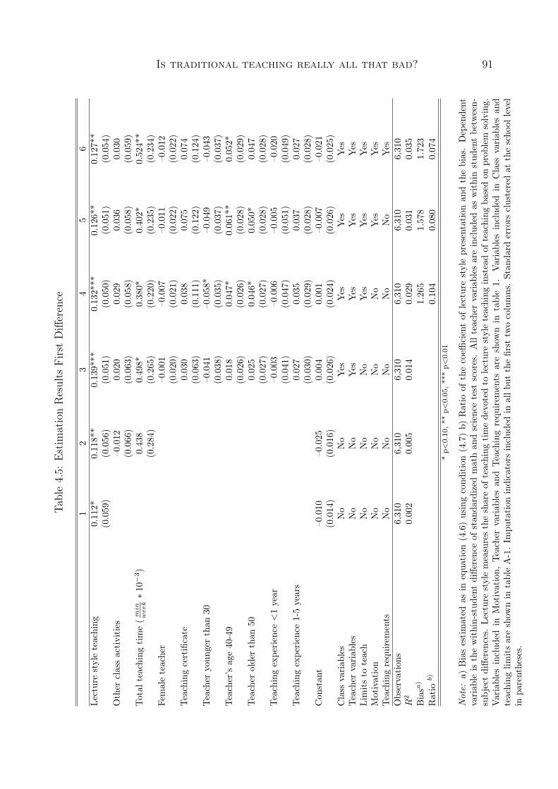
Is traditional teaching really all that bad? 91Ta
ble4.5:
Estim
ationResults
First
Difference
12
34
56
Lecturestyleteaching
0.112*
0.118**
0.139***
0.132***
0.126**
0.127**
(0.059)
(0.056)
(0.051)
(0.050)
(0.051)
(0.054)
Other
classactivities
–0.012
0.020
0.029
0.036
0.030
(0.066)
(0.063)
(0.058)
(0.058)
(0.059)
Total
teaching
time(m
inweek∗
10−3)
0.438
0.498*
0.380*
0.402*
0.524**
(0.284)
(0.265)
(0.220)
(0.235)
(0.234)
Femaleteacher
–0.001
–0.007
–0.011
–0.012
(0.020)
(0.021)
(0.022)
(0.022)
Teachingcertificate
0.030
0.038
0.075
0.074
(0.063)
(0.111)
(0.122)
(0.124)
Teacher
youn
gerthan
30–0.041
–0.058*
–0.049
–0.043
(0.038)
(0.035)
(0.037)
(0.037)
Teacher’s
age40-49
0.018
0.047*
0.061**
0.052*
(0.026)
(0.026)
(0.028)
(0.029)
Teacher
olderthan
500.025
0.046*
0.050*
0.047
(0.027)
(0.027)
(0.028)
(0.028)
Teachingexpe
rience<1year
–0.003
–0.006
–0.005
–0.020
(0.041)
(0.047)
(0.051)
(0.049)
Teachingexpe
rience
1-5years
0.027
0.035
0.037
0.027
(0.030)
(0.029)
(0.028)
(0.028)
Con
stan
t–0.010
–0.025
0.004
0.001
–0.007
–0.021
(0.014)
(0.016)
(0.026)
(0.024)
(0.026)
(0.025)
Class
variab
les
No
No
Yes
Yes
Yes
Yes
Teacher
variab
les
No
No
Yes
Yes
Yes
Yes
Limitsto
teach
No
No
No
Yes
Yes
Yes
Motivation
No
No
No
No
Yes
Yes
Teachingrequ
irem
ents
No
No
No
No
No
Yes
Observation
s6,310
6,310
6,310
6,310
6,310
6,310
R2
0.002
0.005
0.014
0.029
0.031
0.035
Biasa
)1.265
1.578
1.723
Ratio
b)
0.104
0.080
0.074
*p<
0.10,**
p<0.05,***p<
0.01
Not
e:a)
Biasestimated
asin
equa
tion
(4.6)usingcond
ition(4.7)b)
Ratio
ofthecoeffi
cientof
lecturestylepresentation
andthebias.Dep
endent
variab
leis
thewithin-stud
entdiffe
renceof
stan
dardized
mathan
dsciencetest
scores.Allteachervariab
lesareinclud
edas
withinstud
entbe
tween-
subjectdiffe
rences.Le
cturestylemeasurestheshareof
teaching
timedevotedto
lecturestyleteaching
insteadof
teaching
basedon
prob
lem
solving.
Variables
includ
edin
Motivation,
Teacher
variab
lesan
dTeachingrequ
irem
ents
areshow
nin
table1.
Variables
includ
edin
Class
variab
lesan
dteaching
limitsareshow
nin
tableA-1.Im
putation
indicators
includ
edin
allb
utthefirst
twocolumns.Stan
dard
errors
clusteredat
thescho
ollevel
inpa
rentheses.

Is traditional teaching really all that bad? 92
0.1. Our headline estimate is reported in column 6 with an estimated size of 0.1.8 Thisparameter suggests that shifting 10 p.p. of time from problem solving to teaching bygiving lecture style presentations while holding the overall time devoted to these twoactivities constant is associated with an increase in student test scores of one percentof a standard deviation.
In turn, our results imply a negative correlation between more in-class problemsolving and student achievement. This is consistent with the finding in Brewer andGoldhaber (1997) that more in-class problem solving for tenth grade students in mathis related to lower test scores on a standardized test. Furthermore, the other commonlyinvestigated teacher characteristics (e.g. gender, experience, credentials etc.) do notshow significant or robust impacts on student achievement as can be seen in table 4.5.This is in line with previous findings in this literature and emphasizes the importance ofthe statistically significant relationship between more lecture style teaching and studentachievement.
As pointed out in the previous section, estimates might still be biased due to se-lection of teachers into more (or less) lecture style teaching based on unobservableteacher characteristics. This concern is fostered by previous findings in the literaturethat emphasize the importance of unobservable teacher traits for student achievement.This raises the question: How can these results be interpreted?
The bias and ratio at the end of table 4.5 allow us to shed some light on the questionof the influence of unobservables. The underlying assumption for the estimation ofeach bias is that selection on unobservables occurs to the same degree as selectionon observables. In all columns the estimated bias is larger than the point estimateof the impact of lecture style teaching on student test scores. This is reflected inthe ratios at the end of each column that are always smaller than one, indicatingthat selection on unobservables that is weaker than selection on observables sufficesto explain the entire estimated coefficient. In our headline specification in column 6selection on unobservables that is only 0.07 times as strong as selection on observableswould explain the entire estimated coefficient given that the true effect is zero. Onthe one hand, we have included a great amount of control variables so that we believethat selection on unobservables is likely weaker than selection on observables. On theother hand, only very little selection on unobservables compared to the selection onobservables suffices to explain the entire effect. Given this uncertainty, we refrain from
8It should be noted that the lecture style teaching variable is based on self-reported time-use byteachers, which is likely measured with error. If time-use is measured with classical measurementerror, the estimate of the effect of lecture style teaching is biased towards zero. Hence, 0.1 might beinterpreted as a lower bound for the true effect of lecture style teaching.

Is traditional teaching really all that bad? 93
interpreting the results as evidence for a causal effect as the positive coefficient couldalso reflect selection of teachers with desirable unobserved characteristics into lecturestyle teaching.
This raises another question: Why would teachers with different desirable unob-served characteristics select different degrees of lecture style teaching compared toproblem solving? While a reduced form approach of educational production cannotmirror the full complexity of the choices involved in the teaching process, we are,nevertheless, able to pin down the relationship between potential selection based onunobserved teacher traits and the causal effect of lecture style teaching as our estima-tion approach eliminated all other likely biases. If no selection based on unobservableteacher traits exists, our estimates speak for a positive effect of lecture style teaching.Our estimates might, however, be biased upwards if teachers with desirable unobservedcharacteristics more frequently base their instruction on lectures. Theoretically, thisselection bias could be large enough to hide a true negative effect of lecture styleteaching, which would imply that teachers with desirable unobserved characteristicspredominately select themselves into an inferior teaching practice. This scenario, how-ever, lacks any intuitional or theoretical support. We thus argue that this scenario ishighly implausible and can be excluded, which allows a conservative interpretation ofour results: We find no evidence for any detrimental effect of lecture style teaching onoverall student learning.
It is important to stress that our results are limited to student achievement asmeasured by TIMSS test scores.9 Moreover, our results for lecture style teachingare based on a comparison with teaching based on in-class problem solving. Looselyspeaking our results suggest that on average lecture style teaching is at least not worsethan teaching based on in-class problem solving. The comparison of average effectsmight, however, hide significant effect heterogeneities. Depending on the teacher, thestudents, the content taught, or other factors the one or the other teaching practicemight be more effective.
Furthermore, our information on teaching practices, which is based on in-class timeuse reported by teachers, does not allow us to distinguish between different implementa-tions of the teaching practices. One worry might be that especially the implementationof problem-based teaching differs substantially within our sample. Differences betweenthe ideal and the actual implementation of interactive teaching styles that involve moreproblem-based teaching might also reconcile our findings with supportive evidence of
9To the extent that teaching methods cultivate general test-taking abilities differently or generatedifferent long-term effects, a focus on other learning outcomes or on long-term effects might producedifferent results.

Is traditional teaching really all that bad? 94
modern approaches to teaching (Lou et al., 1996; Machin and McNally, 2008). Thus,while a certain teaching practice may be very effective if implemented in the correctway, an empirical analysis that is based on the actual average implementation of thisteaching practice might not reveal any positive effects. Our results, therefore, do notcall for more lecture style teaching in general. The results rather imply that simplyreducing the amount of lecture style teaching and substituting it with more in-classproblem solving without concern for how this is implemented is unlikely to raise overallstudent achievement in math and science.
4.6 Robustness Checks
This section tests the sensitivity of the results presented in section 5 with respect toother definitions of the lecture style variable and with respect to specifications allowingfor heterogeneous effects. The results of these robustness checks are presented in tables4.6 and 4.7.
As our grouping of the response categories available to the teacher in question 20of the 2003 teacher questionnaires in TIMSS could be criticized, we provide evidenceon the effect of interest based on different approaches to construct the lecture stylevariable. We test four alternative definitions of the lecture style variable with corre-sponding estimation results presented in each of the four columns of the upper panelof table 4.6.
In column 1 time spent re-teaching and clarifying content/procedures is includedin the proxy for lecture style teaching. In column 2 taking tests or quizzes is added tothe problem solving category. Hence, the lecture style teaching variable in column 2is defined in relation to the enlarged definition of teaching based on problem solving.In column 3 we decompose the variable other class activities into its elements andseparately control for each category. In column 4 lecture style is defined as the shareof overall time in class spent on giving lecture style presentation.
The coefficients in the upper panel of table 4.6 reveal that redefining our key variableof interest does not change the estimated impact of more lecture style teaching onstudent achievement. While the main purpose of this study is to analyze the teachingof new material by giving lecture style presentations rather than by letting studentssolve problems, it is reassuring to see that increasing the total amount of time in classdevoted to lecture style presentations (in contrast to all other in-class activity) is alsoassociated with higher student achievement.
Additionally, we present evidence for various sub-samples in the middle panel of

Is traditional teaching really all that bad? 95
Table 4.6: Robustness Checks I
Other DefinitionsDef 1 Def 2 Def 3 Def 4
Lecture style teaching 0.145** 0.161** 0.134** 0.156*(0.060) (0.063) (0.054) (0.081)
Observations 6,310 6,310 6,310 6,310R2 0.035 0.036 0.036 0.035
SubsamplesSame Peers Diff Peers No Track Track
Lecture style teaching 0.355*** 0.082 0.116* 0.116(0.118) (0.058) (.070) (.091)
Observations 2,205 4,105 3,529 2,292R2 0.096 0.046 0.065 0.071
Heterogenous effectsDiff Background
Lecture style teaching 0.203*** 0.130*(math) (0.074) (0.072)Lecture style teaching –0.105 –0.111(science) (0.073) (0.071)Observations 6,310 6,310R2 0.065 0.081
* p<0.10, ** p<0.05, *** p<0.01
Note: Dependent variables in all panels and columns are the within-student between-subject dif-ferences in standardized test scores. All teacher variables, class variables, motivation and teachinglimits are included as controls. Upper panel: In Def 1 time spent re-teaching and clarifying con-tent/procedures is added to lecture style teaching. In Def 2 taking tests or quizzes is added toproblem solving. Thus, lecture style teaching in column 2 is defined in relation to the enlarged defini-tion of teaching based on problem solving. In Def 3 the variable ’other class activities’ is decomposedinto its elements and these are separately included to control for each category. Def 4 takes timespent on giving lecture style presentation in relation to all other time-use categories (problem solving+ other class activities). Middle panel: Separate estimation for different sub-samples: Column 1only students with same classmates in both subjects, column 2 students with different classmates.Column 3 students who are tracked according to ability in either both or none of the two subjects,column 4 students who are tracked in at least one of the two subjects. Lower panel: Column 1 and 2allow different coefficients in the two subjects. A negative coefficient for science variables stands for apositive association with the dependent variable. Column 2 additionally includes student backgroundas controls. Imputation indicators are included in all estimations. Standard errors clustered at theschool level in parentheses.
Is traditional teaching really all that bad? 96
table 4.6. In column 1 and 2 we estimate equation (4.5) for students with the same peersin math and science and students with different peers, respectively. This distinctionis motivated by the concern that the main effect might be driven by differences in theclassroom composition. In the sub-sample with identical peers in both subjects ourwithin-student between-subject identification strategy takes care of any potential peereffects. For students with the same peers in both subjects, shifting 10 p.p. of teachingtime from problem solving to lecture style teaching is associated with an increase ofalmost 4 percent of a standard deviation. The estimate in the sub-sample with differentpeers decreases to 0.08 and lacks statistical significance. The results indicate that peereffects do not drive the positive coefficient of lecture style teaching.
Column 3 and 4 of the middle panel of table 4.6 report estimates separately forstudents in schools where either no or both subjects are tracked by ability and forstudents in schools where tracking on ability exists in only one of the two subjects.This distinction is motivated by the consideration that tracking on ability might induceteachers to choose different degrees of lecture style teaching. The results indicate thatthe positive association between more lecture style teaching and student achievementholds in both types of schools. The point estimate is the same for the two groups. Inschools with differential tracking policies, however, it is not statistically significant.
In the lower panel of table 4.6 we investigate subject-specific effects. Column 1and 2 present estimation results from estimating versions of equation (4.4), where weabandon the assumption that coefficients for each right-hand side variable are equalacross subjects. As all science variables enter negatively on both sides of equation(4.4), a negative coefficient for any variable in science masks a positive relationshipbetween the variable and the science test score. All estimates thus have the expectedsigns. They are not statistically significant for science, though. We thus find evidencefor a stronger effect of lecture style teaching in math. A possible interpretation ofthe differential effects in the two subjects is that science with its natural emphasis onexperimentation might just be better suited for problem solving.
So far all specifications measured time devoted to certain class activities in shareswhile additionally controlling for total teaching time. The specification in shares ismainly motivated by the data itself as TIMSS asks teachers to report what percentageof time in a typical week of the specific subject’s lessons students spend on variousactivities. The data also contains information on the total time in minutes per weekteachers teach math or science to the class. Thus, we can also construct a proxy forminutes per week devoted to each activity based on the information on total timeper week and the shares reported by the teachers. While this constructed measure

Is traditional teaching really all that bad? 97
Table 4.7: Robustness Checks II: Absolute Time Specification
Variables are measured as minutes per week spent teaching with specific teaching prac-tice.
(1) (2) (3) (4)Lecture style teaching 0.733* 0.751* 0.653 0.826
(0.426) (0.408) (0.480) (0.526)Problem solving with guidance 0.184 0.174
(0.374) (0.538)Problem solving w\o guidance 0.058 –0.174
(0.424) (0.538)Other class activities 0.444 0.551* 0.362 0.536
(0.315) (0.297) (0.365) (0.461)Total teaching time 0.150 0.236 0.062
(0.293) (0.374) (0.419)* p<0.10, ** p<0.05, *** p<0.01
Note: All teaching practice variables are rescaled as minutes per week divided by (103). Column (1)groups time spent on all activities but lecture style teaching and problem solving, problem solvingwith and without guidance as reference category. Column (2) includes all in-class time use categories,excluded is total minutes per week. Column (3) uses only problem solving with guidance as referencecategory. Column (4) uses only problem solving without guidance as reference category. All speci-fications are otherwise identical to the specification estimated in Column (6) of table 4.5. Standarderrors clustered at the school level in parentheses.
presumably suffers from larger measurement error than the reported shares alone, wenevertheless estimate a version of equation (4.5) that is based on variables indicatingvarious teaching practices measured in minutes per week as a further robustness check.
The results of this robustness check can be seen in table 4.7. All specificationsmeasure class activities in minutes per week. Otherwise the specifications are identicalto the specification estimated in column 6 of table 4.5. In column 1 of table 4.7,minutes spent per week with lecture style teaching and minutes spent on other classactivities are included in the specification while minutes spent on problem solving areexcluded as a reference category. One additional minute per week spent on lecturestyle teaching instead of problem solving is associated with an increase in test scoresof 0.07 percent of a standard deviation. An increase of 23 minutes, which correspondsto a 10 p.p. shift in terms of total teaching time devoted to lecture style teaching, thusresults in an increase in test scores of 1.6% of a standard deviation. This is slightlylarger than our headline estimate based on shares of total teaching time. Column 2 oftable 4.7 reveals that increasing the overall time devoted to lecture style teaching leadsto an increase in test scores of the same magnitude as in column 1 when explicitlyincluding the two problem solving categories and the other class activities. Columns

Is traditional teaching really all that bad? 98
3 and 4 control again for total teaching time, but use either problem solving withthe teachers guidance (column 3) or problem solving without guidance (column 4) asreference categories. The point estimate of lecture style teaching remains positive inboth specifications, but loses significance. The point estimates for the two problemsolving categories in columns 3 and 4 suggest that problem solving with guidanceis slightly more effective than problem solving without guidance. The difference is,however, not statistically significant.10
In sum, we find positive relationships between more lecture style teaching and stu-dent achievement in all robustness analyses. The magnitude of the estimated effectsvaries between specifications and between sub-samples, with insignificant point esti-mates in some specification. Importantly, we do not find evidence for any detrimentaleffect of lecture style teaching in any specification.
4.7 Conclusion
Existing research on teacher quality allows two conclusions: First, there exists a largevariation in teachers’ ability to improve student achievement. Second, this variationcannot be explained by common, observable teacher characteristics. The results pre-sented in this study confirm that these observable teacher characteristics have littlepotential for explaining the variation in student achievement. We provide, however,new evidence on a significant link between teaching practice and student achievement.
The specific teaching practice variable analyzed in this chapter is the share of teach-ing time devoted to lecture style presentation (in contrast to in-class problem solving).We construct this variable based on information on in-class time use provided by teach-ers in the 2003 wave of the Trends in International Mathematics and Science Study(TIMSS) in US schools. Exploiting between-subject variation to control for unobservedstudent traits and estimating a reduced form educational production function, we findthat a 10 percentage point shift from problem solving to lecture style presentationresults in an increase in student achievement of about one percent of a standard devi-ation. We further show that this result is extremely robust to definitional changes inthe construction of the main variable of interest as well as to specifications allowingfor heterogeneous effects.
This finding suggests that students taught by teachers, who devote more teaching10Estimating corresponding specifications to columns 3 and 4 of table 4.7 based on specifications
with lecture style teaching measured in percent of time as in table 4.5 reveals slightly lower estimatesfor the coefficient on lecture style teaching compared to our headline estimate presented in column 6of table 4.5.

Is traditional teaching really all that bad? 99
time to lecture style presentation rather than letting students solve problems on theirown or with the teacher’s guidance, learn more (in terms of competencies tested inthe TIMSS student achievement test). This result stands in contrast to constructivisttheories of learning. It is, however, in line with previous findings in the literature(Brewer and Goldhaber, 1997) showing that instruction in small groups and emphasison problem solving lead to lower student test scores.
We emphasize, however, that our results demand a careful interpretation and needto be taken for what they are: Evidence for a positive association between more timedevoted to lecture style teaching and student achievement that is neither driven byselection of particular students into schools or classes nor by selection of teachersbased on various observable characteristics into a particular teaching method. However,selection based on unobservable teacher characteristics remains a worry. Followingthe method developed in Altonji et al. (2005), we show that only a relatively smallselection based on unobservables suffices to explain the entire estimated coefficient.We thus refrain from formulating any policy conclusions that call for more lecture styleteaching in general.
We are nevertheless able to draw an important conclusion about the nature of thecausal effect of lecture style teaching on student achievement as we eliminated anypotential biases arising from sorting of students, differences in schools and observabledifferences in teacher traits in our empirical approach. The existence of a sizeablenegative causal effect of lecture style teaching would only be consistent with our resultsif teachers with favorable unobserved characteristics predominantly select themselvesinto an inferior teaching practice. Such a scenario, however, lacks any intuitional andtheoretical support. We can thus exclude the possibility of a sizeable detrimental effectof lecture style teaching in math and science instruction on overall student achievementin US middle schools.
We believe that this result is relevant for the debate on optimizing the teachingprocess. Various dimensions of teaching practices have been shown to matter for stu-dent achievement. Moreover, the low-cost implementation of changes in the teachingprocess compared to other policy measures designed to foster student learning makesimprovements in the teaching process particularly appealing. There exists, however,little consensus about what measures could improve the teaching process. Reducingthe amount of traditional instruction based on lecture style teaching is typically a keycandidate. Lectures are potentially connected with many disadvantages and mighttherefore be an inferior teaching method. National standards (NCTM, 1991; NationalResearch Council, 1996) also advocate engaging students more in hands-on learning

Is traditional teaching really all that bad? 100
activities and group work, but traditional lecture and textbook methodologies remaindominant in science and mathematics instruction in US middle schools. This raises theconcern that the high share of total teaching time devoted to traditional lecture presen-tations has a detrimental effect on overall student learning in US middle schools. Ourresults, however, rather imply that, while newer teaching methods might be beneficialfor student achievement if implemented in an ideal way, simply inducing teachers toshift time in class from lecture style presentations to problem solving without concernfor how this is implemented contains little potential to increase student achievement.On the contrary, our results indicate that there might even be adverse effects on studentlearning.

Is traditional teaching really all that bad? 101
Appendix
Selection on unobservables following Altonji et al. (2005)
Formally, in our application the assumption that selection on unobservables occurs to
the same degree as selection on observables as imposed by Altonji, Elder and Taber
(2005) can be stated as:
Proj(∆Lecture|∆Tβ3, η) = φ0 + φ∆T ′β3∆T′β3 + φηη (4.8)
with φ∆T ′β3 = φη (4.9)
Where ∆Lecture captures the between subject differences in the teaching time
devoted to lecture style presentation relative to problem solving and β4 indicates its
coefficient while T includes all other k control variables (teacher characteristics, time
spent on other classroom activities, as well as class characteristics) and β3 is a kx1
vector of coefficients. When ∆T ′β3 is orthogonal to η the assumption (4.9) is equal to
Cov(∆T ′β3,∆Lecture)
V ar(∆T ′β3)=Cov(η,∆Lecture)
V ar(η)(4.10)
We proceed now to answer the question how large selection on unobservables relative
to selection on observabels would have to be in order to explain the entire estimate
of β4 under the assumption that the true β4 is 0. Following Altonji et al. (2005) we
regress ∆Lecture on ∆T , to get
∆Lecture = ∆T ′δ + ˜∆Lecture.
Plugging this into our equation (4.5) yields:
∆Y = c+ ∆T ′(β3 + δ · β4) + ˜∆Lectureβ4 + η (4.11)

Is traditional teaching really all that bad? 102
As ˜∆Lecture is by construction orthogonal to ∆T the probability limit of β4 can
be written as
plim β4 = β4 +Cov( ˜∆Lecture, η)
V ar( ˜∆Lecture)
whereCov( ˜∆Lecture, η)
V ar( ˜∆Lecture)=Cov(∆Lecture, η)
V ar( ˜∆Lecture)
as ∆T is orthogonal to η.
To estimate the numerator of the bias we can use the equality (4.10):
Cov(∆T ′β3,∆Lecture)
V ar(∆T ′β3)· V ar(η).
For this however, we need a consistent estimate of β3 which we obtain by estimating
equation (4.11) under the assumption that β4 = 0.

103
Table 4.8: Descriptive Statistics – Class Characteristics
Math Science359 classes 734 classes
Variable Mean SD Mean SD Difference
Class variablesClass size 23.46 6.54 24.57 7.51 -1.11**Tracked according to ability 0.550 0.480 0.171 0.363 0.379***
Teaching limits (reference not at all/not applicable)Differing academic ability - a little 0.339 0.469 0.340 0.473 -0.002Differing academic ability - some 0.330 0.466 0.321 0.466 0.008Differing academic ability - a lot 0.204 0.399 0.174 0.378 0.031Wide range of backgrounds - a little 0.308 0.456 0.277 0.447 0.031Wide range of backgrounds - some 0.205 0.399 0.238 0.425 -0.032Wide range of backgrounds - a lot 0.060 0.234 0.078 0.267 -0.018Special need students - a little 0.309 0.457 0.328 0.469 -0.019Special need students - some 0.147 0.350 0.184 0.387 -0.037Special need students - a lot 0.064 0.243 0.081 0.272 -0.016Shortage computer hardware - a little 0.140 0.343 0.236 0.423 -0.097***Shortage computer hardware - some 0.197 0.396 0.207 0.404 -0.011Shortage computer hardware - a lot 0.110 0.310 0.189 0.390 -0.079***Shortage computer software - a little 0.168 0.371 0.294 0.454 -0.125***Shortage computer software - some 0.146 0.350 0.198 0.397 -0.052Shortage computer software - a lot 0.145 0.349 0.174 0.378 -0.029Shortage support pc use - a little 0.181 0.380 0.217 0.411 -0.036Shortage support pc use - some 0.148 0.351 0.185 0.387 -0.037Shortage support pc use - a lot 0.089 0.282 0.137 0.343 -0.048*Shortage of textbooks - a little 0.055 0.225 0.088 0.283 -0.034Shortage of textbooks - some 0.045 0.205 0.044 0.205 0.001Shortage of textbooks - a lot 0.011 0.103 0.083 0.275 -0.072***

104
Table 4.9: Descriptive Statistics – Class Characteristics (cont.)
Math Science359 classes 734 classes
Variable Mean SD Mean SD DifferenceShortage instructional equipment - a little 0.180 0.380 0.314 0.463 -0.134***Shortage instructional equipment - a some 0.123 0.326 0.193 0.394 -0.070**Shortage instructional equipment - a lot 0.038 0.190 0.141 0.347 -0.103 ***Shortage demonstrative equipment - a little 0.253 0.431 0.318 0.465 -0.065Shortage demonstrative equipment - some 0.117 0.318 0.196 0.396 -0.080**Shortage demonstrative equipment - a lot 0.044 0.203 0.189 0.391 -0.146***Inadequate physical facilities - a little 0.148 0.352 0.219 0.413 -0.071*Inadequate physical facilities - some 0.051 0.219 0.158 0.364 -0.107***Inadequate physical facilities - a lot 0.030 0.169 0.131 0.337 -0.101***High student teacher ratio - a little 0.230 0.417 0.292 0.454 -0.062High student teacher ratio - some 0.132 0.335 0.204 0.402 -0.071**High student teacher ratio - a lot 0.091 0.285 0.129 0.334 -0.038
Note: Probability weights and within school correlation are taken into account when estimating meansand standard deviations. Class variables are weighted by the number of students in each class.

Bibliography
Aaronson, D., Barrow, L., and Sander, W. (2007). Teachers and student achievementin the Chicago public high schools. Journal of Labor Economics, 25:95–135.
Altonji, J., Elder, T., and Taber, C. (2005). Selection on observed and unobserved vari-ables: Assessing the effectiveness of catholic schools. Journal of Political Economy,113(1):151–184.
Aslam, M. and Kingdon, G. (2007). What can Teachers do to Raise Pupil Achievement?The centre for the study of African economies working paper series.
Atella, V., Brindisi, F., Deb, P., and Rosati, F. (2004). Determinants of access tophysician services in Italy: a latent class seemingly unrelated probit approach. HealthEconomics, 13(7):657–668.
Augurzky, B., Bauer, T. K., and Schaffner, S. (2006). Copayments in the Germanhealth system - Do they work? RWI : Discussion Papers.
Bago d’Uva, T. (2006). Latent class models for utilisation of health care. HealthEconomics, 15(4):329 – 343.
Baker, M., Stabile, M., and Deri, C. (2004). What do Self-Reported, Objective, Mea-sures of Health Measure? Journal of Human Resources, 39(4):1067–1093.
Banerjee, A. V., Cole, S., Duflo, E., and Linden, L. (2007). Remedying education:Evidence from two randomized experiments in India. The Quarterly Journal ofEconomics, 122(3):1235–1264.
Banks, J., Crossley, T., and Goshev, S. (2007). Looking for Private Information inSelf-assessed Health. HEDG Working Paper, University of York 9.
Barrow, L., Markman, L., and Rouse, C. E. (2009). Technology’s edge: The educationalbenefits of computer-aided instruction. American Economic Journal: Economic Pol-icy, 1(1):52–74.

106
Bonesrønning, H. (2004). Do the teachers’ grading practices affect student achieve-ment? Education Economics, 12(2):151–167.
Brewer, D. J. and Goldhaber, D. (1997). Why don’t schools and teachers seem tomatter? The Journal of Human Resources, 32(3):505–523.
Browne, M. and Kamiya, S. (2009). A Theory of the Demand for Underwriting. Work-ing Paper University of Wisconsin-Madison.
Buchmueller, T., Couffinhal, A., Grignon, M., and Perronnin, M. (2004). Access tophysician services: does supplemental insurance matter? Evidence from France.Health Economics, 13(7):669–687.
Bundorf, M., Levin, J., and Mahoney, N. (2008). Pricing and welfare in health planchoice. NBER Working Paper 14153.
Cawley, J. and Meyerhoefer, C. (2010). The Medical Care Costs of Obesity: AnInstrumental Variables Approach. NBER Working Paper 16467.
Cawley, J. and Philipson, T. (1999). An empirical examination of information barriersto trade in insurance. The American Economic Review, 89(4):827–846.
Chatterji, P., Joo, H., and Lahiri, K. (2010). Beware of Unawareness: Racial/EthnicDisparities in Awareness of Chronic Diseases. NBER Working Paper 16578.
Chiappori, P., Jullien, B., Salanie, B., and Salanie, F. (2006). Asymmetric informationin insurance: General testable implications. Rand Journal of Economics, 37(4):783–798.
Cohen, A. and Siegelman, P. (2010). Testing for Adverse Selection in Insurance Mar-kets. The Journal of Risk and Insurance, 77(1):39–84.
Cutler, D., Finkelstein, A., McGarry, K., and Center, L. (2008a). Preference Hetero-geneity and Insurance Markets: Explaining a Puzzle of Insurance. NBER WorkingPaper 13746.
Cutler, D., Lincoln, B., and Zeckhauser, R. (2009). Selection Stories: UnderstandingMovement Across Health Plans. NBER Working Paper 15164.
Cutler, D. and Zeckhauser, R. (2000). The Anatomy of Health Insurance. In Culyer, A.and Newhouse, J., editors, Handbook of Health Economics, volume I, pages 563–643.Elsevier.

107
Cutler, J., Sorlie, P., Wolz, M., Thom, T., Fields, L., and Roccella, E. (2008b). Trendsin Hypertension Prevalence, Awareness, Treatment, and Control Rates in UnitedStates Adults Between 1988-1994 and 1999-2004. Hypertension, 52:818–827.
De Meza, D. and Webb, D. (2001). Advantageous selection in insurance markets.RAND Journal of Economics, 32(2):249–262.
Dee, T. S. (2005). A teacher like me: Does race, ethnicity, or gender matter? AmericanEconomic Review, 95(2):158–165.
Dee, T. S. (2007). Teachers and the gender gaps in student achievement. The Journalof Human Resources, 42(3):528–554.
DeSalvo, K., Bloser, N., Reynolds, K., He, J., and Muntner, P. (2006). MortalityPrediction with a Single General Self-Rated Health Question - A Meta-Analysis.Journal of General Internal Medicine, 21(3):267–275.
Dignath, C. and Büttner, G. (2008). Components of fostering self-regulated learningamong students: A meta-analysis on intervention studies at primary and secondaryschool level. Metacognition and Learning, 3:231–264.
Dixon, J. (2010). The effect of obesity on health outcomes. Molecular and CellularEndocrinology, 316(2):104–108.
Doiron, D., Jones, G., and Savage, E. (2008). Healthy, wealthy and insured? The roleof self-assessed health in the demand for private health insurance. Health Economics,17(3):317–34.
Druss, B., Marcus, S., Olfson, M., and Pincus, H. (2002). The most expensive medicalconditions in America. Health Affairs, 21(4):105–111.
Einav, L., Finkelstein, A., and Cullen, M. (2010a). Estimating Welfare in InsuranceMarkets Using Variation in Prices. Quarterly Journal of Economics, 125(3):877–921.
Einav, L., Finkelstein, A., and Schrimpf, P. (2010b). Optimal mandates and the welfarecost of asymmetric information: evidence from the UK annuity market. Economet-rica, 78(3):1031–1092.
Fang, H., Keane, M., and Silverman, D. (2008). Sources of advantageous selection: Evi-dence from the Medigap insurance market. Journal of Political Economy, 116(2):303–350.

108
Farbmacher, H. (2010). Copayments for doctor visits and the probability of visitinga physician - evidence from a natural experiment. University of Munich WorkingPaper.
Finkelstein, A. and Poterba, J. (2002). Selection effects in the United Kingdom indi-vidual annuities market. The Economic Journal, 112(476):28–50.
Finkelstein, A. and Poterba, J. (2004). Adverse Selection in Insurance Markets: Pol-icyholder Evidence from the UK Annuity Market. Journal of Political Economy,112(1):183–208.
Finkelstein, A. and Poterba, J. (2006). Testing for Adverse Selection with UnusedObservables. NBER Working Paper 12112.
GAO (2003). Private Health Insurance: Federal and State Requirements AffectingCoverage Offered by Small Business. United States General Accounting Office.
Goe, L. (2007). The Link Between Teacher Quality and Student Outcomes: A ResearchSynthesis. Report, National Comprehensive Center for Teacher Quality, WashingtonDC.
Gordon, R., Kane, T. J., and Staiger, D. O. (2006). The hamilton project: Identify-ing effective teachers using performance on the job. Report Washington, DC, TheBrookings Institution.
Gregory, C., Blanck, H., Gillespie, C., Maynard, L., and Serdula, M. (2008). Perceivedhealth risk of excess body weight among overweight and obese men and women:differences by sex. Preventive Medicine, 47(1):46–52.
Grobe, T., Dörning, H., and Schartz, F. (2010). BARMER GEK Arztreport. Schriften-reihe zur Gesundheitsanalyse.
Hanushek, E. (2002). Publicly provided education. In Auerbach, A. and Feldstein, M.,editors, Handbook of Public Economics, volume 4, pages 2045–2141. Elsevier.
Hanushek, E. and Woessmann, L. (2009). Do Better Schools Lead to More Growth?Cognitive Skills, Economic Outcomes, and Causation. NBER Working Paper 14633.
Haslam, D. and James, W. (2005). Obesity. The Lancet, 366(9492):1197–1209.
He, D. (2009). The life insurance market: Asymmetric information revisited. Journalof Public Economics, 93(9-10):1090–1097.

109
Hendel, I. and Lizzeri, A. (2003). The Role of Commitment in Dynamic Contracts:Evidence from Life Insurance. Quarterly Journal of Economics, 118(1):299–327.
Hurd, M. (2009). Subjective probabilities in household surveys. Annual Review ofEconomics, 1:543–562.
Hurd, M. and McGarry, K. (2002). The Predictive Validity of Subjective Probabilitiesof Survival. The Economic Journal, 112(482):966–985.
Idler, E. and Benyamini, Y. (1997). Self-rated health and mortality: a review of twenty-seven community studies. Journal of Health and Social Behavior, 38(1):21–37.
Kan, K. and Tsai, W. (2004). Obesity and risk knowledge. Journal of Health Economics,23(5):907–934.
Kane, T. J., Rockoff, J. E., and Staiger, D. O. (2008). What does certification tell usabout teacher effectiveness? Evidence from New York city. Economics of EducationReview, 27(6):615–631.
Kesternich, I. and Schumacher, H. (2009). On the use of information in repeatedinsurance markets. Discussion paper, SFB/TR 15 Governance and the Efficiency ofEconomic Systems.
Khwaja, A., Silverman, D., Sloan, F., and Wang, Y. (2009). Are mature smokersmisinformed? Journal of Health Economics, 28(2):385–397.
Lichtenstein, S., Slovic, P., Fischhoff, B., Layman, M., and Combs, B. (1978). Judgedfrequency of lethal events. Journal of Experimental Psychology: Human Learningand Memory, 4(6):551–578.
Lo Sasso, A. and Lurie, I. (2009). Community rating and the market for private non-group health insurance. Journal of Public Economics, 93(1-2):264–279.
Lou, Y., Abrami, P. C., Spence, J. C., Poulsen, C., Chambers, B., and d’Apollonia, S.(1996). Wihtin-class grouping: A meta-analysis. Review of Educational Research,66(4):423–358.
Machin, S. and McNally, S. (2008). The literacy hour. Journal of Public Economics,92(5-6):1441–1462.
Manski, C. (2004). Measuring expectations. Econometrica, 72(5):1329–1376.

110
Marmot, M., Banks, J., Nazroo, J., and Blundell, R. (2009). English longitudinal studyof ageing: Wave 0 (1998, 1999 and 2001) and waves 1-3 (2002-2007). 11th Edition.Colchester, Essex: UK Data Archive [distributor] SN: 5050.
Martin, M. E. (2005). TIMSS 2003 User Guide for the International Data Base. Inter-national Association for the Evaluation of Educational Achievement (IEA), Boston.
Matsumura, L. C., Garnier, H. E., Pascal, J., and Valdes, R. (2002). Measuringinstructional quality in accountability systems: Classroom assignments and studentachievement. Educational Assessment, 8(3):207–229.
McCarthy, D. and Mitchell, O. (2010). International Adverse Selection in Life Insuranceand Annuities. In Tuljapurkar, S., Chu, C., Gauthier, A., Ogawa, N., and Pool, I.,editors, Riding the Age Wave, volume 3, chapter 6. Springer.
McTigue, K., Harris, R., Hemphill, B., Lux, L., Sutton, S., Bunton, A., and Lohr, K.(2003). Screening and interventions for obesity in adults: summary of the evidencefor the US Preventive Services Task Force. Annals of Internal Medicine, 139(11):933–966.
Mossialos, E. and Thomson, S. (2009). Private Health Insurance in the EuropeanUnion. Brussels, European Commission (Directorate General for Employment, SocialAffairs and Equal Opportunities).
National Center for Health Statistics (2010). Health, United States, 2009: With SpecialFeature on Medial Technology. Hyattsville, MD.
National Research Council (1996). National science education standards. Report,Washington, DC.
NCTM (1991). Professional standards for teaching mathematics. Report, NationalCouncil of Teachers of Mathematics, Reston, VA.
Oliveira, C. (2008). Nurse Visit - ELSA user day. Presentation at ELSA user day 2008,Economic and Social Data Service.
Poterba, J. (1996). Government Intervention in the Markets for Education and HealthCare: How and Why? In Fuchs, V., editor, Individual and Social Responsibility:Child Care, Education, Medical Care, and Long-Term Care in America, pages 277–308. University of Chicago Press.

111
Propper, C. (1989). An econometric analysis of the demand for private health insurancein England and Wales. Applied Economics, 21(6):777–792.
Risk Classification in Individually Purchased Voluntary Medical Expense Insurance(1999). The American Academy of Actuaries Issue Paper.
Rivkin, S. G., Hanushek, E. A., and Kain, J. F. (2005). Teachers, schools, and academicachievement. Econometrica, 73(2):417–458.
Rothschild, M. and Stiglitz, J. (1976). Equilibrium in Competitive Insurance Mar-kets: An Essay on the Economics of Imperfect Information. Quarterly Journal ofEconomics, 90(4):629–649.
Rouse, C. E. and Krueger, A. B. (2004). Putting computerized instruction to the test:A randomized evaluation of a “scientifically based” reading program. Economics ofEducation Review, 23(4):323–338.
Rückert, I., Böcken, J., and Mielck, A. (2008). Are German patients burdened by thepractice charge for physician visits(’Praxisgebuehr’)? A cross sectional analysis ofsocio-economic and health related factors. BMC Health Services Research, 8(232).
Schacter, J. and Thum, Y. M. (2004). Paying for high- and low-quality teaching.Economics of Education Review, 23(4):411–430.
Schoenbaum, M. (1997). Do smokers understand the mortality effects of smoking? Ev-idence from the Health and Retirement Survey. American Journal of Public Health,87(5):755–759.
Schreyögg, J. and Grabka, M. M. (2010). Copayments for ambulatory care in Germany:a natural experiment using a difference-in-difference approach. European Journal ofHealth Economics, 11(3):331–341.
Scott, A. (2000). Economics of general practice. In Culyer, A. and Newhouse, J.,editors, Handbook of Health Economics, volume 1, pages 1175–1200. Elsevier.
Seidel, T. and Shavelson, R. J. (2007). Teaching effectiveness research in the pastdecade: The role of theory and research design in disentangling meta-analysis results.Review of Educational Research, 77(4):454–499.
Slavin, R. E., Lake, C., and Groff, C. (2009). Effective programs in middle and highschool mathematics: A best-evidence synthesis. Review of Educational Research,79(2):839–911.

112
Smith, J. (2007). Nature and causes of trends in male diabetes prevalence, undiagnoseddiabetes, and the socioeconomic status health gradient. Proceedings of the NationalAcademy of Sciences, 104(33):13225–13231.
Viscusi, W. (1990). Do smokers underestimate risks? Journal of Political Economy,98(6):1253–1269.
Viscusi, W. and Hakes, J. (2008). Risk beliefs and smoking behavior. Economic Inquiry,46(1):49–59.
Weiss, I. R. (1997). The status of science and mathematics teaching in the UnitedStates: Comparing teacher views and classroom practice to national standards. NISEBrief 3, National Institute for Science Education, Madison: University of Wisconsin-Madison.
Wenglinsky, H. (2002). How schools matter: The link between teacher classroompractices and student academic performance. Education Policy Analysis Archives,10(12):1–28.
Winkelmann, R. (2006). Reforming health care: Evidence from quantile regressionsfor counts. Journal of Health Economics, 25(1):131–145.
Wooldridge, J. (2010). Econometric analysis of cross section and panel data. The MITpress, 2 edition.