Empirical analysis of monetary policy: Croatia vs. Slovenia

Munich Personal RePEc Archive

Empirical analysis of monetary policy:

Croatia vs. Slovenia

Vidakovic, Neven

Effectus University College for Finance and Law

2007

Online at https://mpra.ub.uni-muenchen.de/64583/

MPRA Paper No. 64583, posted 25 May 2015 13:48 UTC

55

6

UDK: 336.74:338.26(497.5:497.4)Članek poskuša pojasniti vzročnoodvisnost med izvozom in realnimdeviznim tečajem. V članku avtor razvijeenostaven ekonomski model, ki temeljina odnosu med izvozom in razliko vobrestnih merah, povpraševanjem iztujine po domačem blagu in realnimdeviznim tečajem. Model je empiričnopreverjen za Slovenijo in Hrvaško.Empirična analiza kaže, da je odvisnostmed razlikami v realnih obrestnihmerah, tujim povpraševanjem inizvozom, če sploh obstaja, zelo šibka.Hkrati pa obstaja močna odvisnost medizvozom in realnim deviznim tečajem.Ključna ugotovitev je, da je bilaslovenska politika drsečega deviznegatečaja bistveno uspešnejša od politiketrdnega deviznega tečaja na Hrvaškem.

Ključne besede: realni tečaj, denarnapolitika, izvoz

I z v l e č e k

JEL: F41, E42, O24

Neven Vidaković, BAPrivredna Banka Zagreb andBusiness School »Libertas«

Empirična analiza denarne politike na Hrvaškem in

v Sloveniji

EMPIRICAL ANALYSIS OF MONETARY POLICY:

CROATIA VS. SLOVENIA

VIDAKOVIĆ: EMPIRICAL ANALYSIS OF MONETARY POLICY: CROATIA VS. SLOVENIA

UDC: 336.74:338.26(497.5:497.4)This paper tries to explain empirical cau-sation between exports and the real ex-change rate. The paper develops asimple model based on the relationshipof exports to real interest rate differen-tial, foreign demand for domestic goods,and real exchange rate. The paper thentests the model with empirical data fromCroatia and Slovenia. The empiricalanalysis in the paper finds that there isa very limited relationship between realinterest rate differentials, foreign de-mand and exports. However, there is astrong relationship between exports andthe real exchange rate. When empiri-cally tested, the model confirms that themonetary policy of sliding exchange ratein Slovenia was vastly superior to themonetary policy of fixed exchange ratein Croatia.

Key words: real exchange rate, monetarypolicy, exports

A b s t r a c t

1 The whole process of transition and monetary adjustment is still not over in all countries

of ex-Yugoslavia.

1 Introduction

When Yugoslavia fell apart, what was once a big closed economy becamefive small open economies. Once the military operations and initial instances ofhyperinflation stopped (hyperinflation in Croatia ended in 1994), the succeedingcountries started to build their own economies.1

The process of transformation from a closed socialist system to an openeconomy was complex and challenging. Even fifteen years after the fall ofcommunism, some ex-Yugoslavian republics, such as Bosnia or Serbia andMontenegro, have not made much headway in the transition process. Others, likeSlovenia, are economically closer to western European countries than to othertransition countries. The explanation of these differences presents a challengingtask for any economics research paper.

This paper does not look at all of the aspects of the transition process; it onlylooks at the results of the monetary policies implemented. In effect, the paper isempirically evaluating two different monetary policies implemented, one in Croatiaand the other in Slovenia, with a special focus on exports.

But before we look at the specific history, we should look at the big picture.The main economic problems for the newly formed countries can be formulatedin the following way:

a) How to transition from the socialist fiscal policy (the government ownseverything) to the capitalist fiscal policies of limited (if any) governmentinvolvement? This process had to be done, at least in theory, with the minimumof social cost and maximum social benefit.

b) How to formulate a monetary policy and set up a central monetary authoritywith clearly defined objectives and methods? The main problem with the set-up of the monetary policy was the choice of the optimal monetary policy tool.

This paper does not look into the fiscal policy, privatization, or any other kindof development of the capitalistic free market economies that countries of ex-Yugoslavia have undertaken. Instead, this paper takes a look at two opposingmonetary regimes (Slovenia and Croatia) and tries to create, on an empiricallevel, a study of the real effects of the monetary policy choices.

The fundamental question about monetary policy is the issue of inflation,more specifically the control of inflation. In small open economies with freefluctuation of capital, the control of inflation translates into the control ofexpectations, as presented in Sargent (1992).

The newly founded countries lived under closed socialistic systems with fixedexchange rates (or exchange rates strictly determined by the National Bank ofYugoslavia). Due to the high inflation in the 1980s and the general instability ofthe dinar, most people in ex-Yugoslavia preferred to keep their income and savings

56

NG, ŠT. 1–2/2007 IZVIRNI ZNANSTVENI ČLANKI/ORIGINAL SCIENTIFIC PAPERS

in foreign currency, mostly Deutsch marks. Unlike other ex-socialist countries which had very limited access to hardcurrency, Yugoslavia was a special case. There was a constantinflow of hard currency from tourism and from Yugoslavswho worked in Western Europe.

When Yugoslavia fell apart, the main question for boththe government and the people was: what to do with theexchange rate?

Soon two opposing schools developed. One school ofthought considered it the best to keep the exchange rate fixed.The main argument was that through a stable or fixedexchange rate, the central bank would have an easymechanism for control of the quantity of money in theeconomy and, as such, inflation would be contained. Inaddition, perceptions and expectations of a stable exchangerate would create an expectation of a stable currency withlow inflation. This argument was very important in Croatia,where after the war there was a period of hyperinflation, asdescribed in Rohatinski et al (1995).

The second school wanted to constantly depreciate theexchange rate, or implement a “sliding” exchange rate. Itwas believed that such policies of constant depreciationwould weaken the national currency and stimulate exports,an important part of GDP. For a small open economy, a (real)depreciation and growth of exports can be a considerablesource of economic growth. From a mathematical standpoint, this policy can also be explained as the dynamicprogramming problem of the real exchange rate as presentedin Vidaković (2005b).

In essence, a constant real exchange rate depreciationpolicy was a mercantile “beggar thy neighbor” type policy,but with one major advantage: there was no concern aboutcounterparty depreciation or a trade war. The countries ofthe EU, where most of Croatian and Slovenian exports went,would never just depreciate their currencies as a response toCroatian or Slovenian monetary policy, especially with theMaastricht Treaty and the process of building a currencyunion. On the other hand, the WTO prevents any tariff andcustoms impositions, but does not stipulate anything aboutmonetary policy.

So from a game theory point of view, it was possible toimplement either monetary policy. It was a unique period intime, when two countries had to decide which path to take.The choice was between a path of stability and security (fixedexchange rate); or a path of uncertainty, but with a possiblelarge payoff.2 Many of these dilemmas were presented inRibnikar (1999).

The main problem with the exchange rate for both schoolswas the determination of the transmission of the exchangerate into inflation, meaning: will there be some realdepreciation? And is depreciation going to translate into the

inflation one-for–one, or will there be an overshooting effect?If overshooting was the case, then the argument for thesliding exchange rate would be void. But today we have anopportunity to empirically see the results of two differentpolicies.

This paper looks at a natural experiment which hasoccurred in real life. The two “test subjects” are Sloveniaand Croatia, two similar countries which have taken twodifferent paths. The most interesting aspect of this paper isnot a development of a model in order to artificially test themodel’s assumptions. Rather, the most interesting aspect ofthis paper is the explanation of the results of monetarypolicies in the last 10 years.

One policy was applied in Slovenia, a sliding exchangerate. It was based on a simple rule: depreciate the exchangerate at the same rate as inflation or higher. The exchange ratewas depreciated slowly over time. In essence, it was vectortargeting of the real exchange rate, as we shall see later. Thepath of the vector was set in order to achieve two goals:

a) Depreciate the real exchange rate and thus constantlymake Slovenian products more competitive in the worldmarket.

b) Prevent large capital inflows in Slovenia and thusdecrease foreign debt.

The Croatian strategy was different. After the war inCroatia, there was a period of hyperinflation. At one point,inflation was at 30% per month. Then in 1994 came thestabilization program that ended inflation. In order to keepinflation under control, the HNB (Hrvatska Narodna Banka,Croatian National Bank) decided to keep the exchange rateapproximately the same. HNB stated that its purpose was tokeep the oscillation of the exchange rate to a minimum,reacting to shocks to the exchange rate. This in effect madethe kuna exchange rate a mean reverting series, withoscillations up to 3% from the mean. So the only goal of themonetary policy was the stability of the exchange rate.Monetary policy did not concern itself with exports, imports,foreign debt or any other economic variables, just the stabilityof the exchange rate.

The model in this paper is based on a simple dynamicprogramming optimization of export function in a small openeconomy. Special attention is devoted to the analysis of thereal exchange rate and the impact of the real exchange rateon exports. The model is tested empirically, comparing theresults of the two monetary policies.

The paper is organized as follows: part two develops themodel, part three compares the model and the empirical datawith some interesting results, and part four concludes.

2 The model

When the central banks of Slovenia and Croatia weredetermining their respective policies regarding the exchangerate, the literature on the real exchange rate and openeconomies was relatively small. Up to that time, the mostimportant research done on open economies was Robert

2 In essence, we have an Elsberg paradox as presented in Sargent

and Hansen (2000) as a choice between known and unknown

distribution.

57

Mundell’s (1968) seminal work, and research done by RudyDornbush (1988). Furthermore, some computationaleconomics techniques (forward looking rational expectationsmodels3) had not been developed at that point in time, andcomputer power was low.

Today the state of economic theory regarding openeconomies is unrecognizable from the state of economictheory fifteen years ago. In the last fifteen years, there havebeen many successful attempts in the creation of a workingsmall open economy model, most notably the efforts of Galiet al (2005), Ball (1999), and Rogoff and Obstfeld (2000,2002). There have also been huge advances in thedevelopment of computational techniques as presented inthe works of Ljungqvist and Sargent (2004) and Hansen andSargent (2006).

After the Asian, Mexican, Russian and Argentineancurrency crises, it became apparent that economics as ascience does not fully understand the workings of themechanisms involving the real exchange rate and thetransition from fixed exchange rate to flexible exchange rate.Recently the research of Aizenman and Glick (2005) studiesthe behavior of fixed exchange rates and the transition froma fixed exchange rate to a flexible exchange rate. Aizenmanand Glick analyzed the cost of a switch from a fixed regimeexchange to a flexible regime exchange rate and came to astunning conclusion. Out of the 63 instances of currencyregime switch, 32 were considered disorderly. However, theduration of the regime plays a considerable role. There were20 cases where a fixed exchange regime was longer then200 months. Out of the 20 instances of regime switching, 16had a negative rate of growth and a fall in real output oncethe move to the flexible exchange regime was made, 4 had apositive rate of real output, and one instance was neutral.These results offer a powerful empirical argument against afixed exchange rate regime,4 especially in the long run. Theconclusion of Aizenman and Glick’s paper can be summedup as follows: the longer the fixed exchange rate regime, thelarger is the cost of switching to the flexible regime.

There are several models that try to portray the behaviorof a small open economy. One has been presented in Ball(1999), and many have been presented in the works ofObstfeld and Rogoff. In this paper we will work with amodification of the Mundell-Fleming model explained inVidakovic (2005a). This paper is in effect the continuationof the theoretical base made in Vidakovic (2005a and 2005b).The main model can be shown as follows:

y= c + s + g + (ex – im) (1)

e = c + I + g + (f – d) (2)

c = c°(-r,y) + A + c(y,- r, -E/P, W/P); A= z + φ(y, E/P) (3)

I = i(-r)° + i(CM) – iA*(CM, E/P) = i° + p (4)

im = c(y) + im° ± ζ(CM, E/P) = im° + m (5)

ex = ex°(E/P) + A*(y*) ± ζ (CM, E/P) = ex° + x (6)

g= g° (7)

y – GDPy* – GDP of the rest of the worlde – expendituresc – consumptions – savingsg – government expendituresex – exportsim – importsI – investmentsr – real interest ratesf – Croatian investment in the rest of the worldd – foreign investment in Croatiac° – autonomous consumptionA – Croatian demand for importsW – wagesP – price levelCM – world interest ratesg° – autonomous government expendituresi° – autonomous investmentsex° – autonomous exportsim° – autonomous importsA* – foreign demand for Croatian imports

From the above equations, we can get the IS curve for asmall open economy:

y = c°(-r,y) + c(y,-r, -E/P, W/P) + i°(-r) + g° +

+ im° + ex° + [ A + p + m + x] (8)

For the LM curve, we will use a standard Keynesian LMfunction:

l

lxhyr

π−−

= (9)

Once we graph the two equations, we will get a staticKeynesian small open economy model:


3 Here the author is mostly considering the rational expectations

model presented in Sargent and Hansen (2006)

4 Naturally this argument does not hold if a country has a fixed

exchange rate in order to enter a currency union.

This model, in effect, is the Mundell-Fleming version ofthe IS-LM closed economy model. It is a standard Keynesianstatic macroeconomic model. It is assumed that the labormarket clears and that all changes are instantaneous. The

58

expectations do not enter into the model and time variantprocesses do not play any role, so there are no lag operators.

Obviously this kind of model is not an appropriate ormodern tool in today’s economic theory. Today we havemathematical tools to develop more dynamic models, so weshall work with an updated version of the model.

The theoretical background from Vidaković (2005b) triesto create an optimization of the export function. The basisfor this optimization is the mathematics of dynamicprogramming. The central focus of Vidaković (2005b) is onthe functions:

im = c(y) + im° ± ζ(CM, E/P) = im° + m (10)

ex = ex°(E/P) + A*(y*) ± ζ(CM, E/P) = ex° + x (11)

These two functions represent the static functions forexports and imports in a small open economy. Previous workhas theoretically transformed these functions from static todynamic forms. This transformation has ushered in a modelable to give optimal dynamic account of the export functionfor a small open economy.

2.1 Dynamic model of exports.

In order to develop the model, we will have to makesome assumptions about the model. The first assumptionwill be that there are n households in economy. Althoughthe number of households is large, there is one representativeagent that resembles the rest of the households. The mainproblem the household faces is how to maximize utility overan infinite period of time. Utility comes from consumption:

dtc

t

∫∞

−−

−

−0

11

1max

θ

θ

θ

θβ (12)

Subject to:

∑−

−−

++−=

1

0

1)1(t

i

it

ittttswrswwc τ

0 < β < 1

where w is the wage the household receives, s is constantsavings rate, and τ is the portion of savings households decideto liquidate in period t, 0 ≤ τ ≤ 1. This number is stochasticfor every time period. Function 12 gives us the optimizationproblem for the household given its consumption. But sincewe are dealing with a small open economy it is necessary todefine consumption.

The household has the opportunity to consume two kindsof goods, domestic goods and foreign goods. Equation 13defines such total consumption:

fdh ccc ϑϑ +−= )1( (13)

Where ϑ represents the fraction of goods consumed,totaling 1; subscript d represents the domestic goods andsubscript f represents the foreign goods; and c is the vectorof goods consumed.

If we take the utility function as:

θ

θ

θ

θ

−−

−=

11

1)(

c

cuh (14)

Combining equations 13 and 14 we get:

( ) θ

θ

θ

θ

ϑϑ −−

−

+−=

11

1

)1()(

fd

h

cc

cu (15)

The cost of consumption can be defined as follows:

max ∑∑ +=

n

fii

m

dii ccP

0

,

0

,)*( ψρρ (16)

Subject to ∑−

−−

++−=

1

0

1)1(t

i

it

ittttswrswwc τ , so c=P

for every time period.

The price (P) spent on goods is the sum total of pricespaid for domestic goods plus prices paid for foreign goods;ψ in period t represents the exchange rate; and ρ is the priceof the ith good.

2.2 Factors that have an impact on exports

In order to better understand the optimization of theexport process, we have to define and investigate what factorshave an impact on exports.

According the Mundell-Fleming model presented at thebeginning of the paper, the most important factors affectingexports in a small open economy are:

1. Real exchange rate.2. Capital mobility, caused by the real interest rate differential.3. The economic condition of the country where most of

the exports go.

The reasons for naming each of these variables shouldbe obvious. The real exchange rate presents the true valueof the goods; capital mobility (real interest rate) will serveas an equalizer for the marginal productivity of capital; andthe economic condition of the country that is importing thegoods from a small open economy represents the demandfactor for export products.

The author’s main interest is the analysis of the timevector for each of the three variables presented. Someassumptions are in order. The first one is the assumption ofrational expectations as presented in Muth (1961) and Lucas(1972). The second assumption is the assumption of timeoptimization consistent with the set-up of a dynamicprogramming problem as presented in Stokey and Lucas(1989) and Adda and Cooper (2003). The third assumptionis the assumption of perfect substitution between domesticand foreign goods. This assumption states that arepresentative household is indifferent between the domesticand foreign good as long as the real price is the same. Incase the domestic currency is undergoing a real appreciationover time, consumers will start to substitute for the cheaper


59

foreign goods. This changes the relative values of thedistribution of weight between domestic and foreign goods.

The reader should notice here that there is no mention ofthe nominal exchange rate. This is a very important aspectof this paper. In essence the author of this paper is arguingthat under the above assumptions the nominal exchange rateis irrelevant.

Extrapolating from the argument of Lucas (1972), we seethat any kind of announced exchange rate movements willnot have any kind of real effect on the customer’s preferences.The nominal exchange rate in this paper is considered onlyin relation to the real exchange rate. The effect of changes innominal exchange rate is understood to be neutral in themodel. However, this assumption of neutrality of the nominalexchange rate is tested in the appendix.

Capital mobility is an important factor for the standardof a small open economy. Better real return on capitalinvested can mean movement of jobs from one country tothe next one, thus increasing employment and overallstandard of living in the economy.

With perfect capital mobility, as presented in the model,capital will move to countries where it can obtain a greaterreal interest rate return. The movement of capital in essenceis the capital account balance. In case a country has largeand persistent trade deficits, it will be necessary to financethose deficits. For a country to do that, it has to allow acounter balance in the capital account to offset the currentaccount deficit. This can only be done by selling goods orby selling labor. For the scenarios of trade deficits in thecase of Croatia, see Vidaković (2005a).

The third factor is the demand for export goods, or wecan say the current economic state of the country where theexports go. The rationale for this is simple: if we areexporting in a country with high economic growth, even ifthe percentage of the market held by the exporting countrystays the same, economic growth will cause imports toincrease in nominal quantities, although the percentage inthe market might stay the same. This is the exogenousvariable in the model.

2.3 Real exchange index

The following part of this paper develops an index ofthe real exchange rate and runs simple OLS regressions inorder to establish which of the above noted variables havean impact on the exports and to what extent. The purpose ofthe OLS regression is not to be used as a forecastingmechanism, but to confirm or deny causation and connectionbetween the variables. There will also be a separate test forthe nominal exchange rate.

First we have to create an index of the real exchangerate for Croatia and Slovenia. The notation for the data usedand the process of index creation are in the data appendix atthe end of the paper.

The main purpose of the index is to show in a simpleand straightforward manner the movement of the realexchange though time.

The index of the real exchange in the model is:

( )∏+−

Λ=Φ

t

im

t

ex

t

t

ee0 1

1

(17)

Λ − constant, the beginning value of index 1994 = 100.eex − price change in Croatia or Slovenia (percentage change

or inflation), plus exchange rate appreciation, minusthe exchange rate depreciation in the period.

eim − world inflation, in this case inflation in the EU.

The index created here is very simple. If the index is goingdown, this means that the prices in the domestic country areincreasing more then the prices in the rest of the world. Thismeans that the real exchange rate is appreciating. Domesticgoods are more expensive, foreign goods are cheaper, andthe substitution effect takes place. On the other hand, if theindex is going up, the prices in the rest of the world areincreasing faster then the prices in the domestic country, thereal exchange rate is depreciating, and households will startto substitute foreign goods for domestic goods.

According to the basic theory, the decrease in this indexshould have a negative effect on exports in a small openeconomy.

3 Empirical testing

Before we start the regression analysis, let us look atthe nominal exchange rate for a ten-year period for Croatiaand Slovenia. The exchange rate used is the exchange rateof the HRK vs. the euro and the tolar vs. the euro in theperiod 01/95-01/05.

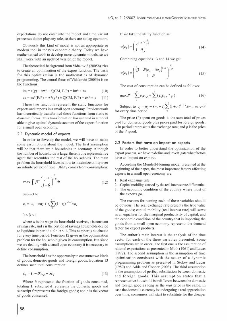
As seen in the graph, it is clear that the kuna exchangerate has been in a very narrow range from the period of mid-1998 until today. The mean for the whole period is 7.28,with a standard deviation of 0.33. The minimum in the seriesis 6.61 and the maximum is 7.73. The lower bound is 0.67kuna away from the mean of about 9%. The upper bound is0.45 kuna away from the mean of 6%, essentially indicatingan upward resistance.

The graph shows that since the beginning of 1999 thekuna has been heavily controlled. The exchange rate is notfixed, but it has been kept in a very narrow band. Now giventhe theory of the model, such an economic behavior shouldbe negative for the exports in Croatia if there exists aconsiderable price differential between Croatia and thecountry that imports Croatian goods.

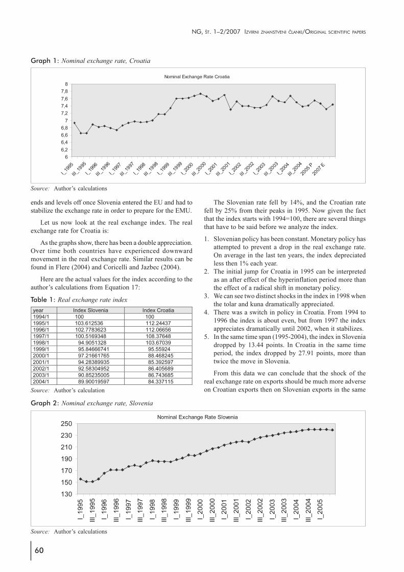
The same analysis can be done with the tolar. The meanof the series is 201.783. The highest point is 239.99 and theminimum of the series is 150.78. It should be noted that theminimum value occurs at the beginning of the series, andthe highest value occurs towards the end of the series.

It can be clearly seen that there is a persistent nominaldepreciation of the exchange rate of the tolar vs. the euro.

The first observation from these two graphs should be theway the graphs look. The kuna is a straight line, while thetolar is almost a linear function with a steady slope. The slope


60

ends and levels off once Slovenia entered the EU and had tostabilize the exchange rate in order to prepare for the EMU.

Let us now look at the real exchange index. The realexchange rate for Croatia is:

As the graphs show, there has been a double appreciation.Over time both countries have experienced downwardmovement in the real exchange rate. Similar results can befound in Flere (2004) and Coricelli and Jazbec (2004).

Here are the actual values for the index according to theauthor’s calculations from Equation 17:

The Slovenian rate fell by 14%, and the Croatian ratefell by 25% from their peaks in 1995. Now given the factthat the index starts with 1994=100, there are several thingsthat have to be said before we analyze the index.

1. Slovenian policy has been constant. Monetary policy hasattempted to prevent a drop in the real exchange rate.On average in the last ten years, the index depreciatedless then 1% each year.

2. The initial jump for Croatia in 1995 can be interpretedas an after effect of the hyperinflation period more thanthe effect of a radical shift in monetary policy.

3. We can see two distinct shocks in the index in 1998 whenthe tolar and kuna dramatically appreciated.

4. There was a switch in policy in Croatia. From 1994 to1996 the index is about even, but from 1997 the indexappreciates dramatically until 2002, when it stabilizes.

5. In the same time span (1995-2004), the index in Sloveniadropped by 13.44 points. In Croatia in the same timeperiod, the index dropped by 27.91 points, more thantwice the move in Slovenia.

From this data we can conclude that the shock of thereal exchange rate on exports should be much more adverseon Croatian exports then on Slovenian exports in the same


Source: Author’s calculations

Graph 1: Nominal exchange rate, Croatia


Graph 2: Nominal exchange rate, Slovenia

Source: Author’s calculation

Table 1: Real exchange rate index

61

time period, under the assumption that real exchange ratehas an effect on exports. This assumption still has to beproven empirically.

Going back to Equation 15, we see utility is based onconsumption, and from equation 16 we see that if domesticgoods are becoming cheaper, households will substituteforeign goods for domestic goods. From the results in thereal exchange rate movement, we can conclude thesubstitution effect in Croatia should be much more adverseto domestic production than in Slovenia.

3.1 Regressions

Now we will run regressions on several variables to seethe overall impact of real exchange rate, interest ratedifferential, and foreign demand for exports. We will bedealing with the basic one step ordinary least squaresregression of the form:

ex = α + β1γ + β

2δ + β

3ε

γ − log value A*δ − log value ξε − log value Φ

The purpose of this regression is not to be able to predictthe future movement of the real exchange rate or to serve asa model. Much better and more accurate results for prediction

can be obtained using VAR methods as in Echebaum andChristiano (2005) or a recently developed FAVAR procedureas proposed by Bernanke et al (2005). Rather OLSregressions here are being used to be able to determine withstatistical significance which of the variables have an impacton exports and which variables do not have impact onexports. The three main variables that we are focusing onare: real exchange rate (as presented in the index above),interest rate differential, and growth in the country whereCroatia and Slovenia export, in this case growth in the EU.

The regression results here are for Croatia. The regressionresults for Slovenia are in the appendix.

The most striking result of regression was the fact thatthe interest rate differential and growth in the EU were notstatistically significant.

ex = 10.37 – 5.72γ – 4.188δ + 0.536ε

(13.32) (-0.52) (-1.01) (3.59)

The t-statistic values are in brackets.

As we can see, neither interest rate differential nor growthis significant. The only statistically significant element ofthe equation is the real exchange rate index. From this theconclusion follows that in order to increase exports, a countryshould depreciate the real exchange rate.



Graph 3: Real exchange rate, Croatia


Graph 4: Real exchange rate, Slovenia

62

There is also a possible problem with the small samplesize, but since the time period considered is small, the 40observations are the only observations possible.

From this regression we can move to the single factorregression, and regressing only the values of exports on theindex of real exchange rate we get:

ex = 10.1625 + 0.5514ε

(13.84) (3.79)

Again the real exchange rate index is extremelysignificant and confirms the assumptions of the model.

In fact it is very significant and R square is at 26%, arelatively high R square for only a one variable regression.Also keep in mind that these are log values, so a positivesign in front of â makes sense. As the index goes up by 1percent, the exports will go up by 0.55 percent.

The results for Slovenia are very similar to those obtainedfor Croatia and are shown in the appendix with the rest ofthe results.

3.2 Discussion

The testing of data rejects the theoretical implications inVidakovic (2005b). Vidakovic (2005b) states that thereshould be three main variables for the stimulation of exports;however, empirical testing rejects that hypothesis and leavesus with only one variable: real exchange rate.

The only realistic policy for a small open economy is tokeep depreciating the real exchange rate. Through realdepreciation of the exchange rate, a small open economy inessence forces households to substitute domestic for foreigngoods.

But there are two problems with this logic:

1. The first problem is the fact that the real exchange ratecannot be constantly depreciated. The reason for this isthe autonomous imports. We are dealing with a small openeconomy and there are some imports that a small openeconomy needs in order to function properly, and thereare some goods where the substitution effect is impossible.The autonomous imports are part of eEquation 5.

2. The second reason is the nature of the problem. It is notpossible to set a goal for the depreciation of the real exchangerate forever. Such constant depreciation of real exchangerate in a linear or on an exponential (by constant percentage)basis seems highly implausible in the real world.

But there is a solution to the problem. A small openeconomy cannot constantly depreciate its currency adinfinitum, but a small open economy can optimize the realdepreciation/appreciation, which we have empirically seenin the case of Slovenia. The real exchange index isappreciating, but through proper monetary policy the realdepreciation has been slowed and put under control. On theother hand, in the case of Croatia we are seeing a lack ofdefined monetary policy. There is only preservation of thestatus quo: a fixed exchange rate no matter what the cost. InCroatia’s case, the real exchange rate has been left to drift

widely, and due to the considerable interest rate differential,this has caused massive foreign debt and a huge currentaccount deficit.

3.3 Solution

As we can see from the regressions, the most importantfactor for growth in imports is the real exchange rate. So inorder for an economy to have growth in exports, it isnecessary to optimize the real exchange rate.

However, the real exchange rate is not just a variablethat can be easily changed. If we look at equation 17, we seethat prices in the exporting country are beyond our control.In essence, controlling the real exchange rate is a stochasticdynamic programming problem. Such a problem can berepresented in the value equation 18.

)'()(max)('

exVEcuexVexex

β+= (18)

Empirically, if we look at the exchange rate indices forCroatia and Slovenia, we see that the real exchange indexfor Slovenia is a solution to Equation 18.5 Although the indexis not moving in the desired direction (the index isappreciating instead of depreciating), we see that the indexis smooth with very small volatility. Croatia’s real exchange,on the other hand, is wild and volatile.

3.4 Results

This is an empirically oriented research paper and now weshall look at the empirical results of the monetary policy chosen.Looking at the model, the main prediction is that due tooscillations in the real exchange rate, a substitution effect willtake place. If the real exchange rate is appreciating, domesticgoods will increase in price and force rational households tosubstitute domestic for foreign goods. This substitution effectwill cause large persistent trade deficits and in case there is areno alternate domestic means to finance the deficit, the countrywill have a large increase in foreign debt.

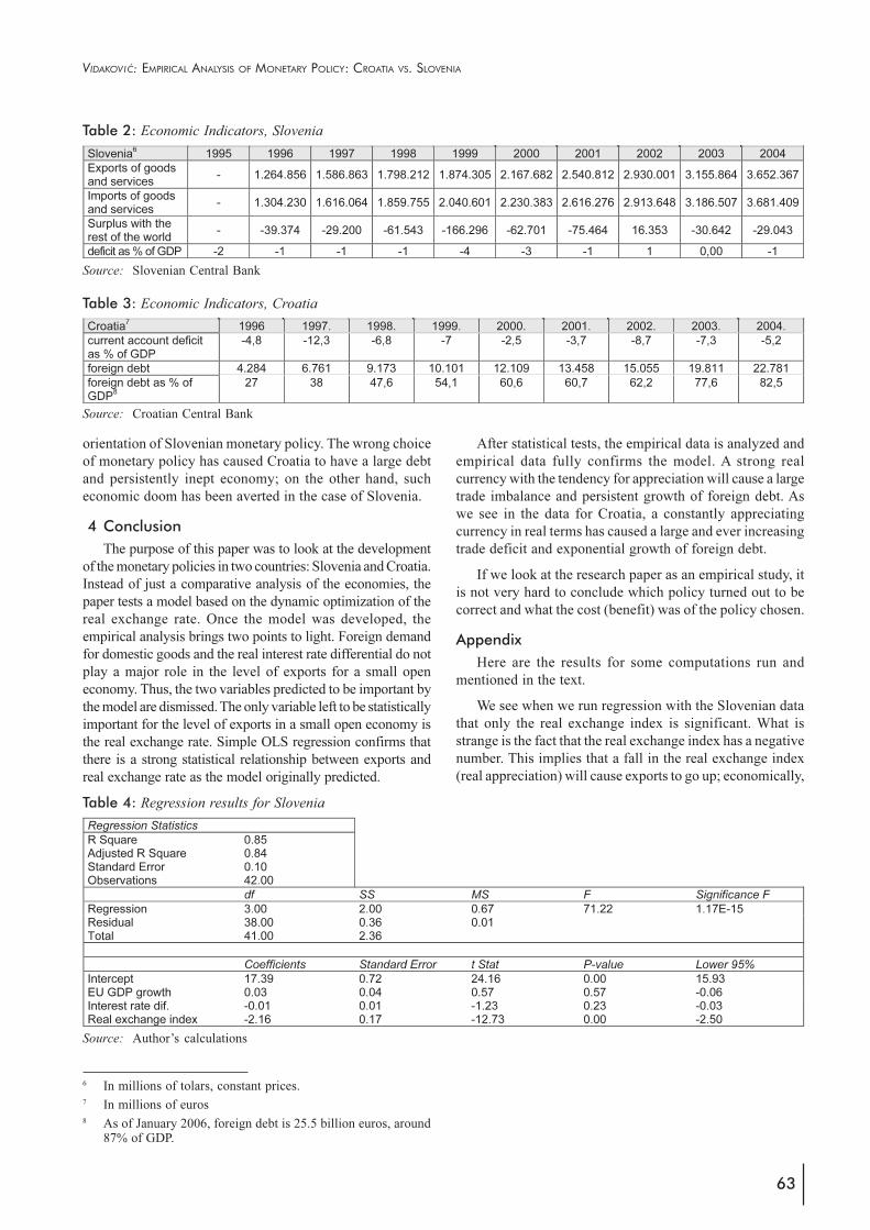
From the data we have seen on real exchange rate, themodel tells us that Slovenia should have a small trade deficitand small foreign debt. On the other hand, Croatia, accordingto the model, should have a large trade deficit and largeforeign debt. Now we shall look at the data and see if themodel’s predictions are correct.

In the last ten years, Croatia has undergone a persistenttrade deficit and foreign debt has exploded, as can be seenfrom the data below. During the same time period, Sloveniahas had a stable balance of payment and relatively benignforeign debt.

Thus, the model is absolutely correct in its predictionsabout the effect of the real exchange rate on the trade balanceand foreign debt.

As we see, the empirical data has shown the wrongorientation of Croatian monetary policy and the correct


5 By solution, the author here means smoothness of the curve

and small standard deviation of the index, not the mathematical

properties of the dynamic programming value equation solution.

63

orientation of Slovenian monetary policy. The wrong choiceof monetary policy has caused Croatia to have a large debtand persistently inept economy; on the other hand, sucheconomic doom has been averted in the case of Slovenia.

4 Conclusion

The purpose of this paper was to look at the developmentof the monetary policies in two countries: Slovenia and Croatia.Instead of just a comparative analysis of the economies, thepaper tests a model based on the dynamic optimization of thereal exchange rate. Once the model was developed, theempirical analysis brings two points to light. Foreign demandfor domestic goods and the real interest rate differential do notplay a major role in the level of exports for a small openeconomy. Thus, the two variables predicted to be important bythe model are dismissed. The only variable left to be statisticallyimportant for the level of exports in a small open economy isthe real exchange rate. Simple OLS regression confirms thatthere is a strong statistical relationship between exports andreal exchange rate as the model originally predicted.


After statistical tests, the empirical data is analyzed andempirical data fully confirms the model. A strong realcurrency with the tendency for appreciation will cause a largetrade imbalance and persistent growth of foreign debt. Aswe see in the data for Croatia, a constantly appreciatingcurrency in real terms has caused a large and ever increasingtrade deficit and exponential growth of foreign debt.

If we look at the research paper as an empirical study, itis not very hard to conclude which policy turned out to becorrect and what the cost (benefit) was of the policy chosen.

Appendix

Here are the results for some computations run andmentioned in the text.

We see when we run regression with the Slovenian datathat only the real exchange index is significant. What isstrange is the fact that the real exchange index has a negativenumber. This implies that a fall in the real exchange index(real appreciation) will cause exports to go up; economically,

Source: Slovenian Central Bank

Table 2: Economic Indicators, Slovenia

Source: Croatian Central Bank

Table 3: Economic Indicators, Croatia

6 In millions of tolars, constant prices.7 In millions of euros8 As of January 2006, foreign debt is 25.5 billion euros, around

87% of GDP.


Table 4: Regression results for Slovenia

64

this does not make any sense. This can be explained in twoways:

1. Statistically the regression is correct. In the time periodtested, the index is falling and exports are rising, so theregression coefficient should be negative.

2. The nominal value of the exchange rate is important,although in the paper we have assumed households onlycare about the real value of variables, not just nominalvalues.

Running a one variable regression, we again obtain anegative coefficient on the long index, but this time thecoefficient is much smaller (-0.39 versus -2.16 from theprevious regression). Also in this regression the t-statistic ismuch larger.

The next regression is the regression of nominal valueof exports on the nominal value of the exchange rate. As wecan see, regression is statistically significant and the values

of the t statistic are extremely large in the case of Slovenia,but in the case of Croatia we do not get this result.

In the case of Croatia, the same regression is not valid,the t statistic is small, and the nominal exchange rate isinsignificant even at the 10% level test. The p value is 13%.So we can conclude that the nominal exchange rate andexports are not correlated. This is an extremely powerfulconclusion that completely supports the main argument ofthe paper: only the real exchange rate matters.

What these two regressions tell us is that Slovenianexports are growing not because the exchange rate is falling,but because the real exchange rate is being controlled throughdepreciation. On the other hand, in Croatia there is noexchange rate movement due to any factor, so the relationshipbetween the exchange rate and exports is not statisticallysignificant.






Table 6: Regression results for Croatia


65

Bibliography

1. Adda, Jerome and Cooper, Russell (2003). Dynamic

Economics: Quantitative Methods and Applications. MITPress.

2. Aizenman, Joshua and Glick, Reuven (2005). PeggedExchange Rate Regimes - A Trap? NBER Working Paper

w11652.3. Ball, Laurence (1999). Policy Rules for Open Economies.

In Monetary Policy Rules, ed. John Taylor. Universityof Chicago Press.

4. Ben S. Bernanke, Jean Boivin and Piotr Eliasz (2005).Measuring the Effects of Monetary Policy: A Factor-Augmented Vector Autoregressive (FAVAR) Approach.Quarterly Journal of Economics 120 (1): 387-422.

5. Christiano, Lawrence, Eichenbaum, Martin andVigfusson, Robert (2005). Assessing Structural VARs.Working paper, Northwestern University.

6. Coricelli, Fabrizio and Jazbec, Bostjan (2004). Realexchange rate dynamics in transition economies. Structural

Change and Economic Dynamics 15 (1): 83-100.7. Dornbush, Rudy (1988). Open Economy

Macroeconomics: New Directions. In Misalignment of

Exchange Rates, ed T.R. Marston , University of ChicagoPress.

8. Flere, Luka (2004). Realni Efektivni Devizni TečajTolarja in Konkurenčnost. Prikazi in analize XII/1.Central Bank of Slovenia Ljubljana.

9. Gali, Jordi and Monacelli, Tommaso (2005). MonetaryPolicy and Exchange Rate Volatility in a Small OpenEconomy. Review of Economic Studies, 72 (3): 707-734.

10. Lucas, Robert E. Jr. and Sargent, Thomas J (1981). AfterKeynesian Economics. In Rational Expectations and

Econometric Practice, eds Robert E. Lucas, Jr. and ThomasJ. Sargent. Minneapolis: University of Minnesota Press.

11. Lucas, Robert E., Jr. (1972). Expectations and theNeutrality of Money. Journal of Economic Theory 4 (1):103–124.

12. Mundell, Robert (1968). International Economics. NewYork : Macmillan.

13. Muth, John F. (1961). Rational Expectations and the Theoryof Price Movements. Econometrica 29 (6): 315–335.

14. Obstfeld, Maurice and Rogoff, Kenneth (2000). NewDirections for Stochastic Open Economy Models.Journal of International Economies 50 (2): 117-153.

15. Obstfeld, Maurice and Rogoff, Kenneth (2002). The SixMajor Puzzles in International Macroeconomics: Is Therea Common Cause? NBER Working Paper w 7777.

16. Ribnikar, Ivan (1999). Monetary arrangements andexchange rate regime in a small transitional economy(Slovenia). In Inclusion of Central European countries

in the European Monetary Union, eds, Paul de Grauweand Vladimir Lavrač. Boston: Dordrecht; London:Kluwer Academic Publishers.

17. Rohatinski, Željko; Anušić, Zoran; Šonje, Velimir (1995).Put u Nisku Inflaciju. Vlada Republike Hrvatske.

18. Rogoff, Kenneth, Reinhart, Carmen, and Savastano,Miguel (2003). Debt Intolerance. Brookings Papers on

Economic Activity 1: 1-62.19. Stokey, Nancy, and Lucas, Jr., Robert E. (with Edward

C. Prescott) (1989) Recursive Methods in Economic

Dynamics. Cambridge, Mass.: Harvard University Press.20. Sargent, Thomas (1992). Rational Expectations and

Inflation. New York: Harper and Row, second edition.21. Sargent, Thomas and Ljungqivst, Lars (2004). Recursive

Macroeconomic Theory. Second Edition, MIT Press.22. Sargent, Thomas and Hansen, Lars (2000). Wanting

Robustness in Macroeconomics. June unpublished.23. Sargent, Thomas; Hansen, Lars (2006). Robustness.

unpublished book manuscript.24. Vidaković, Neven (2005a). Mundell-Fleming Model and

its Applicability on a Small Open Economy. Ekonomija

11 (3): 392-424.25. Vidaković, Neven (2005b). Theory of Rational Expectations

and Exports. Ekonomija 12 (1): 153-173.


Empirical analysis of monetary policy: Croatia vs. Slovenia

Documents

Transcript of Empirical analysis of monetary policy: Croatia vs. Slovenia