EMPAX-CGE Model Documentation - US Environmental Protection

March 2008

EMPAX-CGE Model Documentation

Interim Report

Prepared for

U.S. Environmental Protection Agency Office of Air Quality Planning and Standards

Research Triangle Park, NC 27711

Prepared by

RTI International Health, Social, and Economics Research


RTI Project Number 0209897.002.041

RTI Project Number 0209897.002.041

EMPAX-CGE Model Documentation

Interim Report

March 2008

Prepared for

U.S. Environmental Protection Agency Office of Air Quality Planning and Standards


Prepared by

RTI International* Health, Social, and Economics Research


*RTI International is a trade name of Research Triangle Institute.

ACKNOWLEDGEMENTS

The EMPAX-CGE model was developed for the Innovative Strategies and Economics Group (ISEG) under EPA contract number 68-D-99-024 by RTI International’s Center for Regulatory Economics and Policy Research in Research Triangle Park, NC. Tom Walton, Larry Sorrels, and Lisa Conner of ABC, and previously Tyler Fox, Linda Chappell, and Arturo Rios of ISEG, were the EPA project managers. Special thanks to EPA ISEG staff and to Martin Ross, Brooks Depro, and Robert Beach of RTI International for their efforts in developing this tool and its documentation.

iii

CONTENTS

Section Page

1. Introduction .............................................................................................................. 1-1 1.1 Background...................................................................................................... 1-1

1.2 History of CGE Modeling ................................................................................ 1-2 1.3 Application of CGE Models to Environmental Policies .................................... 1-3

1.4 Overview of a Standard CGE Model ................................................................ 1-5 1.5 Summary of EMPAX-CGE Features ................................................................ 1-8

1.6 Outline of Model Documentation ..................................................................... 1-9

2. Overview of EMPAX-CGE....................................................................................... 2-1

2.1 General Structure ............................................................................................. 2-1 2.2 Households ...................................................................................................... 2-2

2.3 Trade................................................................................................................ 2-4 2.4 Production Activities........................................................................................ 2-4

2.5 Tax Rates and Distortions ................................................................................ 2-5 2.6 Government and Investment............................................................................. 2-5

2.7 Industries in EMPAX-CGE (Static Versions) ................................................... 2-6 2.8 Regions in EMPAX-CGE (Regional Static Version) ........................................ 2-8

2.9 Social Accounting Matrix................................................................................. 2-9 2.10 Policy Evaluation ............................................................................................. 2-9

3. EMPAX-CGE Modeling Framework ........................................................................ 3-1 3.1 Production........................................................................................................ 3-1

3.1.1 Electricity Generation ........................................................................... 3-5 3.1.2 Manufacturing, Nonmanufacturing, and Services .................................. 3-8 3.1.3 Fixed Resource Sectors (Agriculture and Fossil Fuels).......................... 3-8

3.2 Households .................................................................................................... 3-12

3.3 Trade.............................................................................................................. 3-16

iv

3.4 Government and Investment........................................................................... 3-18 3.5 Market Clearing ............................................................................................. 3-18

4. Database and Calibration........................................................................................... 4-1 4.1 Social Accounting Matrix................................................................................. 4-1

4.2 IMPLAN Economic Data ................................................................................. 4-3 4.3 Energy Data Sources ........................................................................................ 4-4

4.4 Energy Data Calibration................................................................................... 4-5 4.4.1 Step 1: Estimate Energy Use for EMPAX-CGE Sectors....................... 4-5 4.4.2 Step 2: Determine National Energy Forecasts....................................... 4-7 4.4.3 Step 3: Allocate National Energy Data to States................................... 4-8 4.4.4 Step 4: Aggregate State-level Data to Regions and Balance Trade

Flows.................................................................................................... 4-8 4.5 Data Integration in the SAM............................................................................. 4-9

5. Model Calibration and Policy Evaluation .................................................................. 5-1 5.1 Model Calibration ............................................................................................ 5-2

5.2 Environmental Policy Evaluation ..................................................................... 5-2

6. Dynamic Version of EMPAX-CGE........................................................................... 6-1

6.1 Data Used by the Dynamic Version of EMPAX-CGE ...................................... 6-2 6.2 Energy Use ...................................................................................................... 6-4

6.3 Natural Resources ............................................................................................ 6-6 6.4 Capital Stock and Adjustment Dynamics.......................................................... 6-7

6.5 Households ...................................................................................................... 6-8 6.6 Generation of a Baseline Model Solution ......................................................... 6-9

7. Taxation in EMPAX-CGE ........................................................................................ 7-1 7.1 Overview ......................................................................................................... 7-1

7.2 Labor Taxes ..................................................................................................... 7-2 7.3 Capital Taxes ................................................................................................... 7-3

7.3.1 Theoretical Approach............................................................................ 7-3 7.3.2 Data and Estimated Capital Tax Rates................................................... 7-9

7.4 Labor Supply Decisions and Tax Distortions.................................................. 7-14

v

References ........................................................................................................................ R-1

Appendixes

A: Features of Selected CGE Models ................................................................... A-1 B: Linkage Between EMPAX-CGE and the Integrated Planning Model............... B-1

C: List of Industries in the National Static Version of EMPAX-CGE ................... C-1

vi

LIST OF FIGURES

Number Page

1-1. Circular Economic Flows within CGE Models .......................................................... 1-6

2-1 General EMPAX-CGE Structure............................................................................... 2-3 2-2 Regions in EMPAX-CGE ......................................................................................... 2-8

3-1 General Production Structure .................................................................................... 3-3 3-2 Electricity Generation ............................................................................................... 3-4 3-3 Energy Use in Fossil-Fueled Electricity Generation .................................................. 3-5 3-4 Energy Use in Manufacturing, Nonmanufacturing, and Service Sectors .................... 3-6 3-5 Structure of Agricultural Production........................................................................ 3-10 3-6 Structure of Natural Resources Production (Coal, Crude Oil, Natural Gas).............. 3-11 3-7 Petroleum Refining Structure .................................................................................. 3-12 3-8 Household Utility Function ..................................................................................... 3-14 3-9 Trade Functions ...................................................................................................... 3-17

5-1 Flow Chart of Steps in Developing and Applying a CGE Model ............................... 5-1

6-1 Regions in EMPAX-CGE (Dynamic Version)........................................................... 6-4 6-2 AEO’s Changes in Energy Use for Selected Fuels/Industries..................................... 6-5

vii

LIST OF TABLES

Number Page

2-1 Dimensions of EMPAX-CGE Versions ..................................................................... 2-2 2-2 Characterization of Industries in EMPAX-CGE (Regional Static Version) ................ 2-7

3-1 General Production Elasticities.................................................................................. 3-2 3-2 Elasticities Related to Energy Use in Electricity and Manufacturing/Services ........... 3-6 3-3 Elasticities Related to Resource Sectors .................................................................... 3-9 3-4 Elasticities Related to Household Consumption and Trade ...................................... 3-13

4-1 Basic SAM................................................................................................................ 4-2 4-2 EMPAX-CGE Economic Data Sources ..................................................................... 4-3 4-3 EMPAX-CGE Energy Data Sources.......................................................................... 4-6

5-1 Distributions of Environmental Protection Expenditures for Selected Industries........ 5-4

6-1 Industries in Dynamic Version and Correspondence to Static Version....................... 6-3 6-2 Industrial Output Revenues (in millions of $2005) .................................................. 6-12 6-3 Energy Consumption by Sector in the United States (Quadrillion BTU).................. 6-13 6-4 Energy Consumption by Components of Energy-Intensive Manufacturing

(Quadrillion BTU) .................................................................................................. 6-14

7-1 Wage and Salary Data by State: 2005....................................................................... 7-3 7-2 Average Marginal Effective Income Tax Rates by Type and State: 2005.................. 7-5 7-3 Parameter Definitions (following FR notation).......................................................... 7-6 7-4 Exogenous Variable Values (following FR notation)................................................. 7-7 7-5 Corporate Marginal Tax Rates by State: 2005 .......................................................... 7-9 7-6 Equipment and Structures Assets: Corporate and Noncorporate Sectors ................. 7-11 7-7 Inventory and Land Assets: Corporate and Noncorporate Sectors........................... 7-11 7-8 Regional Tax Rates ................................................................................................. 7-12 7-9 Cost Data by Type of Capital .................................................................................. 7-13 7-10 U.S. Industry Capital Stocks and Weighted Average Marginal Effective Capital

Tax Rates ................................................................................................................ 7-15 7-11 Weighted Average of Fullerton Corporate and Noncorporate METR....................... 7-16 7-12 MCPF and MEB Estimates in the Dynamic Version of EMPAX-CGE .................... 7-17

1-1

CHAPTER 1 INTRODUCTION

Computable general equilibrium (CGE) models are widely used in policy analysis, including analyses of environmental issues. For environmental policies that are expected to affect many sectors either through direct compliance costs or indirectly through linkages between sectors of the economy (i.e., industries, households, government, trade), it may be important to account for these interactions and constraints. General equilibrium (GE) models account for these linkages and are more appropriate than partial equilibrium analysis of large regulations that are expected to have measurable impacts across the economy. This report describes the CGE version of Economic Model for Environmental Policy Analysis-Computable General Equilibrium version (EMPAX-CGE), which was specifically designed for use in analyses of large-scale environmental regulations.

1.1 Background EMPAX-CGE is a regional CGE model developed by RTI International (RTI) for the

Environmental Protection Agency’s Office of Air Quality Planning and Standards (OAQPS). It is designed to estimate regional macroeconomic impacts of environmental regulations on the United States’ economy. Many major regulations directly affect a large number of industries and/or substantially affect markets for key factors of production. In either case, substantial indirect impacts may result from changes in production, input use, income, and consumption patterns for directly affected markets. EMPAX-CGE offers the ability to trace economic impacts as they are transmitted throughout the economy and allows it to provide insights to policy makers evaluating the magnitude and distribution of costs associated with environmental policies.

The EMPAX model was first developed in 2000 to support the economic analysis of EPA regulations controlling hazardous air pollutant emissions from three combustion source categories (reciprocating internal combustion engines, boilers, and turbines).1 It was a national multimarket partial equilibrium model with linkages between manufacturing industries and the energy sector designed to capture the effects that these combustion rules will have on other sectors of the economy through impacts on energy prices and output. A modified version of EMPAX was subsequently used to analyze the impacts of air pollution control strategies under

1Beach, R.H., M.P. Gallaher, B.M. Depro, and A.C. O’Connor. “Economic Impact Analysis of the Reciprocating Internal Combustion Engines NESHAP.” Prepared for the U.S. Environmental Protection Agency, February 2004.

1-2

the Southern Appalachian Mountain Initiative (SAMI).2 Over time, EMPAX has been greatly enhanced through the addition of multiple U.S. regions, more manufacturing and nonmanufacturing sectors; linkages between all sectors; more detailed energy and economic data; an improved characterization of production and consumption; and, in 2003, conversion to a GE framework (i.e., EMPAX-CGE). A key factor common across all versions of the model is the emphasis on capturing interactions between the energy sector and the rest of the economy.

EMPAX-CGE was most recently applied to estimate the macroeconomic effects of the Interstate Air Quality Rule (subsequently renamed the Clean Air Interstate Rule).3 EPA/OAQPS expects to employ it to evaluate economic impacts as part of its review of the National Ambient Air Quality Standards (NAAQS) for particulate matter as well as other future EPA rulemakings.

1.2 History of CGE Modeling Over the last several decades, CGE modeling has emerged as a widely accepted method

for conducting empirical economic analyses because it provides the ability to integrate economic theory with real-world data. The theoretical foundation of these models is a Walrasian general equilibrium structure (Arrow and Debreu, 1954). A “general equilibrium,” as described by an Arrow-Debreu model (see Arrow and Hahn, 1971), includes components such as (1) households in the economy that have an initial endowment of factors of production and a set of preferences for goods; (2) market demands that are the sum of all agents’ demands and depend on prices; (3) solution prices that conform to Walras’ law (expenditures equal income for any set of prices, or more specifically, as a consequence of assuming non-satiation, for any set of prices the value of excess demands over all markets is zero); (4) producers that maximize profits and have constant- or decreasing-returns-to-scale production functions; and (5) an equilibrium solution characterized by prices and production levels such that demand equals supply for all commodities, income equals expenditures, and production activities break even at solution prices (in the case of constant-returns-to-scale production). By combining this theoretical structure with numerical methods, CGE models can be used to estimate the effects of policy changes on all parts of the economy.

Advances in numerical simulation techniques have allowed modelers to move from simple partial equilibrium models to GE models with many more sectors and complex behaviors. This research began with Leontief (1936, 1951, 1953) who developed static input-output (I/O) models. The I/O approach employed “fixed coefficients” that did not allow production technologies to change in response to different policies. Johansen (1960) was the first to develop

2Beach, R.H., and B.M. Depro. “Competitiveness Analyses of Alternative SAMI Strategies.” Prepared for the U.S. Environmental Protection Agency, March 2002.

3 “Regional Macroeconomic Analysis of the Interstate Air Quality Rule.” U.S. EPA, Office of Air Quality Planning and Standards. See www.epa.gov/clearair2004.htm.

1-3

an applied GE model that moved away from this fixed-coefficients assumption to production functions that allow substitution among inputs and technical change. Since then, ever more complex models have been used to investigate a wide variety of policies from taxes to trade to the environment.

Analyses of the incidence and efficiency effects of taxes are based on the seminal works of Harberger (1959, 1962, 1966, 1974). The 1962 work laid out a two-sector GE model of taxes using standard neoclassical assumptions: supplies of capital and labor are fixed, factors are perfectly mobile across industries, and perfect competition exists in product and factor markets. Shoven and Whalley (1972, 1973) were the first to analyze taxes using a full GE structure. Subsequent works, notably Ballard et al. (1985), extended previous models by adding more sectors and modeling dynamic consequences of policies for household savings behavior. Recent works (e.g., Bovenberg and Goulder [1996], Babiker, Metcalf, and Reilly [2002], and Bovenberg, Goulder, and Gurney [2003]) have examined how existing tax distortions in an economy may interact with economic policies and alter their effects.

CGE models have been applied extensively to trade policies due to their ability to examine implications for many industries and countries simultaneously. Deardorff and Stern (1981) developed one of the first large-scale CGE trade models. It had 34 countries and 29 industries and was used to investigate the effects of changes in tariff and nontariff barriers in the Tokyo Round. Analysis of more recent trade agreements, such as the North American Free Trade Agreement (NAFTA) and the Uruguay Round of trade negotiations, have relied heavily on CGE models for assessments of impacts. These studies include U.S. International Trade Commission (1992), Francois and Shiells (1994), Martin and Winters (1996), Robinson et al. (1991), and Burfisher, Robinson, and Thierfelder (1994).

1.3 Application of CGE Models to Environmental Policies As in other branches of economics, the use of CGE models in environmental policy

applications has been growing in recent years as improvements in model structures, databases, and computer technology have reduced the costs of using these models and increased the benefits (see Adkins and Garbaccio [1999] for a bibliography of CGE models applied to environmental issues and IEC [2001] and Appendix A of EPA [2003] for an overview of selected CGE models used in environmental analysis). Regulations may affect the economy through their influence on rates of technological innovation, the level of private investment and trade, and the location decisions of firms and workers. A major strength of CGE models for regulatory analysis is their ability to implicitly take these effects into account. Regulations that directly raise costs of production and/or prices in an industry can indirectly discourage both investment in and exports from that industry as well as industries that rely on that sector for productive inputs. In CGE models, regulatory compliance costs lead to reductions in investment as a result of lower returns

1-4

to capital while exports are discouraged by higher terms of trade (the ratio of domestic to world prices).

The energy sector plays a unique role as an input into essentially every other sector of the economy while simultaneously being one of the largest contributors to air pollution. As a result of its importance, one of the earliest areas of application of CGE models to environmental issues, beginning in the mid- to late-1980s, was to energy policy modeling (e.g., Bergman [1988]; Despotakis and Fisher [1988]). Subsequently there has been an emphasis on the energy sector in almost all CGE models used to analyze large-scale environmental regulations. Often, the energy sector bears a large share of the direct costs, and resulting changes in prices and quantities in the energy market can have a substantial impact on the rest of the economy.

Another early application of CGE models to environmental policy (and still one of the most common) was in the analysis of economy-wide impacts associated with restrictions on or required reductions for emissions of pollutants. Environmental standards, taxes, or tradable permits lead to direct costs, including payments to government (in the case of taxes or auctioned permits), permit trade expenditures, and abatement expenditures. However, direct costs do not necessarily measure social costs nor the distributional implications that are important to policy makers/agencies who seek to design optimal policies from a societal viewpoint. To estimate the social costs of environmental programs, one must capture the sum of direct, indirect, and induced costs.4 This means modeling all relevant linkages, substitution possibilities, technical changes, and dynamic processes that are affected by environmental programs throughout the economy. The CGE framework has proven to be a valuable tool for capturing these kinds of complex effects because of its ability to model individual agent behavior, while at the same time depicting the workings of an entire economy. The Intertemporal General Equilibrium Model (IGEM), developed by Jorgenson, Ho, and Wilcoxen, is an example of a CGE model that has been used in many different studies of the impact of environmental regulations on economic growth since the early 1990s (e.g., Ho and Jorgenson [1998]; Jorgenson [1998]; Jorgenson and Wilcoxen [1990a], [1990b], [1993a], [1993b], [1993c], [1993d], [1997], [1998]) as well as an assessment of the social costs associated with the Clean Air Act. Hazilla and Kopp (1990) used a model that is very similar to IGEM in an analysis of the social costs of the Clean Air and Clean Water Acts.

CGE models have also routinely been applied to evaluate impacts of climate change policies. Studies include Rose and Oladosu (2002), Bernstein et al. (1999), Harrison and Rutherford (1998), Jorgenson and Wilcoxen (1993b), McKibbin et al. (1999), Manne and Richels (1997), and Bovenberg and Goulder (1996), among others. Most of these models

4In the terminology used by input-output models, direct effects are experienced by a specific industry. Indirect effects capture how direct effects spill over into other industries, and induced effects cover how income changes from direct/indirect effects affect the economy.

1-5

provide results at the national level, but efforts have been made to model impacts on different regions of the United States. The Multi-Region National (MRN) model, which is a dynamic CGE model that has been used primarily to estimate impacts associated with various energy policies and hypothetical carbon target policies (Balistreri and Rutherford, 2001), is capable of providing results down to the state level through a decomposition of estimation into three separate models solved sequentially.

Since the mid-1990s, numerous studies have relied on CGE models to examine the interaction between environmental regulations and tax-induced distortions in the labor market, often referred to as tax-interaction effects (TIEs). Parry (1997), Goulder et al. (1999), and Fullerton and Metcalfe (2001) are notable examples of this literature. If one performs single-market analysis of a tax policy, say, or an environmental regulation, then one assumes that there are no other-market distortions or that the exacerbation and amelioration of other-market distortions caused by the intervention in question cancel one another out. The TIEs literature argues that in the case of environmental policy (as well as agricultural policy and trade policy; see Parry [1999] and Williams [1999]) the other-market effects do not cancel out. In particular, the nature of environmental regulation—through command and control, pollution taxes, or quota restrictions on pollution—systematically worsens the distortion in the labor market that arises from the existing income tax (i.e., any decrease in the real wage tends to further decrease labor supply from an already nonoptimal point). This literature has potentially important implications for the way that social costs of environmental regulations are calculated. The findings in this literature argue for the use of CGE models rather than single-sector models in estimation of the social costs associated with regulation to account for the potentially large tax interaction effects that may result.

Some more recent studies are attempting to account for environmental benefits within CGE models. Perroni and Wigle (1994) argue that it is essential to build the benefits of environmental improvement into CGE models. In their model, there is an initial endowment of environmental quality, some of which is consumed by activities that generate pollution. Firms can abate pollution by substituting other inputs (e.g., machinery) for emissions. The household utility function in this model includes environmental quality as a consumption good with increasing marginal utility as income rises. They use the model to explore the interactions between trade policy and environmental policy. Another example of this line of research is Smith et al. (2003), where the benefits of ozone reductions in the Los Angeles Air Basin are estimated in a general equilibrium framework.

1.4 Overview of a Standard CGE Model CGE models explicitly capture all of the flows of factors and commodities in an

economy. Unlike I/O analyses, which focus on the production side of the economy and rely on

1-6

exogenous multipliers to estimate demand effects, CGE models include income flows, distributional effects, and changes in behavior in response to price changes. By modeling both producer and consumer behavior, CGE models are able to estimate how policy effects will ripple through the entire economy in a manner consistent with economic theory.

Figure 1-1 illustrates a simplified version of the circular flows in an economy considered by a CGE model.5 Households own factors of production (capital, labor, and natural resources) and supply them to firms. These factor sales generate income for households. Firms produce output by combining productive factors with intermediate inputs of goods and services from other industries. Output of each industry is purchased by other industries and consumers using the income received from sales factors. Goods and services can also be exported, and imported goods can be purchased from other countries.

Imports Exports

FirmsHouseholds

Factors ofProduction

Householdspurchase goods

& servicesFirms buy

goods & servicesas inputs

Firms supplygoods &services

Firmspurchase

factors

Householdssupply factors

Householdsreceive income

from factorsales

Goods &Services

Figure 1-1. Circular Economic Flows within CGE Models

5Although this diagram ignores government, investment, and some features of foreign agents for the sake of simplicity, CGE models usually cover these interactions as well.

1-7

The “general equilibrium” component of CGE modeling requires a comprehensive market coverage in which all sectors in the economy are in balance and all economic flows are accounted for. Every commodity that is produced must be purchased by firms or consumers within the United States or exported to foreign consumers. Prices of these goods reflect all costs of production. Households receive payments for their productive factors and transfers from the government (not shown in Figure 1-1), and this income must equal consumer expenditures. In aggregate, all markets must clear, meaning that supplies of commodities and factors must equal demand, and the income of each household must equal its factor endowments plus any net transfers received.

Firms in a CGE model are assumed to maximize profits, which are the difference between revenues from sales and payments for factors of production and intermediate inputs. Profit maximization is done subject to constraints imposed by available production technologies. According to economic theory of producer behavior, firms will use each type of input up to the point where the marginal revenue received from employing an additional unit of an input is equal to the marginal cost of purchasing that input (i.e., MRP = MC).

Typically, production technologies are specified using constant elasticity of substitution (CES) functions that describe how different types of inputs can be substituted for each other (as discussed in Chapters 2 and 3). The extent of these substitutions is determined by elasticities that control how easily trade-offs among inputs can be made. Unlike I/O models or partial-equilibrium models using fixed coefficients in production, this model structure allows producers to change the technology employed to manufacture goods. If, for example, energy prices rise, an industry can shift away from energy by employing more capital, labor, or intermediate inputs as allowed for by the CES equations. This allows a CGE model to consider energy efficiency improvements as businesses substitute away from energy and into less energy-intensive methods.

Households are assumed to maximize utility received from consumption of goods and services, subject to their budget constraint. CES equations, or other types of functions (e.g., Translog or Generalized Leontief), are used to describe these utility functions, which show how willing and able households are to substitute among consumption goods in response to price changes. Because of the explicit treatment of consumer preferences (in terms of utility or expenditure functions), CGE models are generally able to estimate how a policy will affect consumers’ standard of living as measured by changes in welfare, or Hicksian equivalent variation (EV). Models without a strong theoretical basis are only able to examine changes in variables like gross domestic product (GDP), which may be unrelated to consumers’ standard of living.

1-8

1.5 Summary of EMPAX-CGE Features Several versions of EMPAX-CGE have been developed for EPA:

• two static versions (national and regional) for investigating long-run policy effects on a wide range of industries (THESE TWO VERSIONS ARE IN THE PROCESS OF BEING UPDATED AND COMPLETED), and

• a dynamic regional version to examine policies with varying effects over time (COMPLETED).

The theoretical structures of all versions are similar, although the dynamic version has fewer sectors and regions because of computational constraints and the need for additional features to model investment decisions and energy markets over time (i.e., production, consumption, and price forecasts). Both the static and dynamic versions are described in detail in the following chapters.

The model structure and underlying databases of all EMPAX-CGE versions are designed to be capable of estimating macroeconomic impacts of environmental regulations on different industries and regions in the United States. Although the theoretical structure of EMPAX-CGE is similar to other CGE models looking at energy policies, it includes additional regional information and uses a wide range of sources for its energy data. The regional disaggregation is essential because many environmental policies can have substantially different impacts across areas of the country. Use of the most complete data sources to characterize energy production and consumption by firms and households is also critical when modeling policies that may have significant implications for energy markets.

Aside from dynamics, the main difference between the static and dynamic versions of EMPAX-CGE is the level of aggregation. The national-level static version has 384 sectors, while the regional static version has 82 commodities (seven of which are types of energy), produced by 81 sectors in 10 regions. The dynamic version of EMPAX-CGE has 35 sectors (six of which are types of energy) and five regions. Computational issues limit its size to fewer industries and regions than the static model because the dynamic version uses a perfect-foresight framework and hence must solve for multiple time periods simultaneously, which significantly increases the size of the model. All versions of the model are built using the same dataset and characterizations of firm and household behavior. Responses in the static version are intended to represent long-run changes in the economy, while the dynamic version is able to examine transitional effects as the economy responds to policies over a period of years.

Distortions associated with the existing tax structure in the United States have been included in EMPAX-CGE (as detailed in Chapter 7). A wide range of theoretical and empirical literature has examined “tax interactions” and found that they can substantially alter costs of

1-9

environmental (and other) policies. The economic database used by EMPAX-CGE (as detailed in Chapter 4) includes information on some types of taxes, which have been combined with other sources to cover important distortions from capital and income taxes.

To characterize households, the IMPLAN database was used to distinguish nine groupings classified by income. Because environmental policies can potentially influence income distributions and affect households in substantially different ways, these data can be used to define several households in each region of the model. The static versions of EMPAX-CGE are capable of running all nine household groupings, while computational issues limit the dynamic regional version to four households in each of five regions.

1.6 Outline of Model Documentation The remainder of this report includes the following:

• Chapter 2—Summarizes the EMPAX-CGE model structure, scope, and types of policy evaluations that can be conducted.

• Chapter 3—Discusses additional details of producer and consumer behaviors and presents more information on production technologies of different industries.

• Chapter 4—Examines the data sources used by EMPAX-CGE and how the energy data are integrated with the economic data.

• Chapter 5—Describes the use of EMPAX-CGE for policy applications. It also presents information on how EMPAX-CGE allocates environmental protection expenditures across types of equipment purchases and factor inputs by businesses in order to reduce emissions.

• Chapter 6—Discusses the extensions that have been made to the static version of EMPAX-CGE to incorporate dynamic responses over time.

• Chapter 7—Covers the inclusion of taxes in the model. This allows EMPAX-CGE to consider how interactions between existing taxes and environmental policies may affect model results.

• Appendix A—Summarizes the features of selected CGE models (IGEM and Argonne Multi-sector Industry Growth Assessment Model [AMIGA]) and EMPAX-CGE.

• Appendix B—Shows the various methods by which EMPAX-CGE can be linked to the Integrated Planning Model (IPM) model to estimate macroeconomic effects of electricity policies. It also illustrates the User Interface that automates a linkage between EMPAX-CGE and the IPM and AirControlNet models, and allows the user to determine how EMPAX-CGE will be run.

• Appendix C—Presents the 384 sectors that are included in the national static version of EMPAX-CGE.

2-1

CHAPTER 2 OVERVIEW OF EMPAX-CGE

This chapter provides an overview of EMPAX-CGE covering the general theoretical structure, industry and regional characterizations, and data sources. Subsequent chapters provide additional details on each of these topics.

2.1 General Structure The theoretical framework used by EMPAX-CGE is an Arrow-Debreu general

equilibrium. Firms maximize profits subject to technology constraints, and consumers maximize utility subject to budget constraints. All markets must clear so that supply of goods and services is equal to demand. In addition, income of each agent must equal their factor endowments plus any net transfers.

EMPAX-CGE combines a variety of economic and energy data sources (as detailed in Chapter 5) to characterize energy production and consumption decisions with sufficient regional and industry detail to allow investigation of policies that may alter these decisions. These data are contained in a social accounting matrix (SAM) that shows current production technologies and demands by agents in the economy. The economic data in the SAM come from state-level information provided by the Minnesota IMPLAN Group,1 while the energy data come from the Energy Information Administration (EIA) at the Department of Energy. .

The three versions of EMPAX-CGE employ these data sources to describe regions, industries, and commodities according to the dimensions shown in Table 2-1 (note: as of March 2008, the two static versions of EMPAX-CGE are still in process – this version of the documentation covers the updated data/forecasts used in all versions and their application in the dynamic version of the model, which has been used on the Ozone 070 RIA). The national static version of EMPAX-CGE has been developed for policy investigations that require a substantial level of detail in the representation of manufacturing industries without a need for regional detail (see Appendix C for a complete list of included sectors). The regional static version of EMPAX-CGE uses available data sources to describe 81 sectors and 82 commodities. It includes 10 regions covering the United States, which are combinations of states selected to approximate regions defined as distinct electricity markets by the North American Electric Reliability Council (NERC). Although the dynamic version of EMPAX-CGE contains fewer regions and industries because of computational limits (5 and 35, respectively), the underlying database and model structure are the same. Consequently, although the discussions in Chapters 2 and 3 focus on the

1See http://www.implan.com/index.html for a description of the IMPLAN Group and their data.

2-2

regional static version, the model structure for the dynamic version is substantially similar (differences are highlighted in Chapter 6).

Table 2-1. Dimensions of EMPAX-CGE Versions Version Regions Industries Commodities

Static

National 1 384 385

Regional 10 81 82

Dynamic

Regional 5 35 36

The baseline data used by static EMPAX-CGE are benchmarked using EIA forecasts to represent the economy in a particular year in the future, usually 2015 or 2020. From this starting point, it estimates long-run economic effects for a policy in question. The dynamic model uses baseline data representing the economy in 2005 and solves in 5-year increments out to 2050. For years following 2005, the dynamic version incorporates energy consumption and production forecasts generated by EIA.

All versions of EMPAX-CGE employ a nested CES model structure. These types of nested equations are used by CGE models to portray the types of substitution possibilities available to producers and consumers. Figure 2-1 illustrates this general framework and gives a broad characterization of the model. The diagram begins at the top with household decisions on consumption, followed by the trade structures used to generate aggregate consumption goods from domestic and imported varieties, and finally covers the production functions that provide the goods. Subsequent discussion gives more details about the decisions at each level of the figure, and Chapter 3 provides specifics about the production and consumption functions used.

2.2 Households As appropriate, each region within EMPAX-CGE contains one or more representative

households. As shown at the top of Figure 2-1 (i.e., Level 1), the household(s) maximizes utility received from consumption of goods and leisure time. Income used to purchase goods comes from sales of factors owned by the households, which include capital, labor and natural resources. In Level 2, consumption goods are first divided between transportation services (either purchased or provided through personal vehicles). In Level 3, households decide between energy and consumption and among various consumption goods according to a Cobb-Douglas specification. This structure allows households to shift consumption of goods and services in response to policies. If a good’s price increases, consumers can purchase less of that good and more of other types of goods. Effects of a policy on households’ standard of living (or, more

2-3

formally, their welfare as measured by changes in Hicksian equivalent variation) are determined by how willing and able they are to alter their consumption patterns.

Figure 2-1. General EMPAX-CGE Structure Note: The number of goods depends on the version of EMPAX-CGE being used (statistics shown in Figure 2-1

refer to the dynamic version of the model).

Leisure Consumption

Consumption is a Cobb-Douglas composite of transportation plus goods.

Foreign Domestic Domestic goods are a CES composite of local goods and goods from other U.S. regions.

Local Output

Regional Output

Intermediates KLE

Most producer goods use fixed proportions of intermediate inputs and KLE.

Energy Value Added

Labor Capital Energy

(5 Types)

KLE is a CES composite of energy (E) and value-added (KL).

Value added is a Cobb-Douglas composite of capital and labor (KL).

Utility

Intermediate inputs are the 30 types of non-energy goods, in fixed proportion for each industry.

Energy

Consumption of energy is a CES composite of energy and other consumption goods.

Energy (E) is a CES composite of 5 energy types. The structure of this function varies across industries.

Imports are a CES composite across foreign supply sources.

Purchased Transport

Personal Transport

Transportation Consumption Goods

Petroleum

Services Manufactured Goods

Goods and Services

Transportation is a CES composite of personal vehicle transport and purchased transport.

Personal vehicles use fuel and goods/services.

Each consumption good is a CES composite of foreign and domestically produced goods.

(30 types) (5 types)

Household utility is a CES function of consumption and leisure.

Level 1

Level 2

Level 3

Level 4

Level 5

Level 6

Level 7

Level 8

2-4

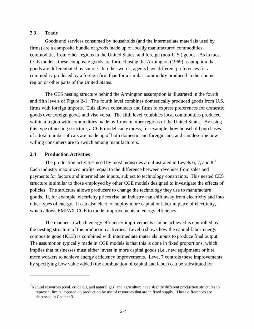
2.3 Trade Goods and services consumed by households (and the intermediate materials used by

firms) are a composite bundle of goods made up of locally manufactured commodities, commodities from other regions in the United States, and foreign (non-U.S.) goods. As in most CGE models, these composite goods are formed using the Armington (1969) assumption that goods are differentiated by source. In other words, agents have different preferences for a commodity produced by a foreign firm than for a similar commodity produced in their home region or other parts of the United States.

The CES nesting structure behind the Armington assumption is illustrated in the fourth and fifth levels of Figure 2-1. The fourth level combines domestically produced goods from U.S. firms with foreign imports. This allows consumers and firms to express preferences for domestic goods over foreign goods and vise versa. The fifth level combines local commodities produced within a region with commodities made by firms in other regions of the United States. By using this type of nesting structure, a CGE model can express, for example, how household purchases of a total number of cars are made up of both domestic and foreign cars, and can describe how willing consumers are to switch among manufacturers.

2.4 Production Activities The production activities used by most industries are illustrated in Levels 6, 7, and 8.2

Each industry maximizes profits, equal to the difference between revenues from sales and payments for factors and intermediate inputs, subject to technology constraints. This nested CES structure is similar to those employed by other CGE models designed to investigate the effects of policies. The structure allows producers to change the technology they use to manufacture goods. If, for example, electricity prices rise, an industry can shift away from electricity and into other types of energy. It can also elect to employ more capital or labor in place of electricity, which allows EMPAX-CGE to model improvements in energy efficiency.

The manner in which energy efficiency improvements can be achieved is controlled by the nesting structure of the production activities. Level 6 shows how the capital-labor-energy composite good (KLE) is combined with intermediate materials inputs to produce final output. The assumption typically made in CGE models is that this is done in fixed proportions, which implies that businesses must either invest in more capital goods (i.e., new equipment) or hire more workers to achieve energy efficiency improvements. Level 7 controls these improvements by specifying how value added (the combination of capital and labor) can be substituted for

2Natural resources (coal, crude oil, and natural gas) and agriculture have slightly different production structures to represent limits imposed on production by use of resources that are in fixed supply. These differences are discussed in Chapter 3.

2-5

energy. The eighth level then determines how capital and labor can be substituted for each other and, in the nest of the seven different types of energy, specifies how one type of fuel can be used in place of another.3

The ease with which firms can switch among production inputs is controlled by elasticities of substitution. Elasticities relating to energy consumption are particularly important for the types of policies investigated by EMPAX-CGE. If, for instance, an industry is able to substitute away from energy with relative ease, the price of its output will not change much when energy prices vary. These elasticity assumptions, which are based on empirical estimation and modeling research by Massachusetts Institute of Technology’s (MIT’s) Joint Program on the Science and Policy of Global Change, are discussed in more detail in Chapter 3.

2.5 Tax Rates and Distortions Taxes and associated distortions in economic behavior have been included in EMPAX-

CGE because theoretical and empirical literature found that taxes can substantially alter estimated policy costs. The IMPLAN economic database used by EMPAX-CGE includes information on taxes such as indirect business taxes (all sales and excise taxes) and Social Security taxes. However, IMPLAN reports factor payments for labor and capital at their gross-of-tax values, which necessitates use of additional data sources to determine personal income and capital tax rates. Chapter 7 describes this process and resulting model estimates of the burden imposed on households by the current tax structure in the United States.

2.6 Government and Investment Government purchases and use of investment goods to form capital stocks are tracked in

the IMPLAN economic data used by EMPAX-CGE (as detailed in Chapter 4). All government expenditures are financed by tax receipts and transfers from households. Although investment behavior plays an important role in the dynamic version of EMPAX-CGE (as detailed in Chapter 6), in the static versions of EMPAX-CGE, investment decisions are not linked to the formation of capital for future production. Therefore, in the static versions of the model, investment goods and government expenditures are determined from the IMPLAN data and are maintained at their current baseline levels and do not enter the optimization decisions of households and businesses. In all versions of the model, government purchases (as measured in real terms using the cost of obtaining the desired bundle of goods) are maintained through non-distortionary lump-sum transfers between the government and households. In the dynamic version of EMPAX-CGE, it is not necessary to exogenously maintain investment-goods purchases since decisions on investment and capital stocks are a result of the model, rather than an exogenous input.

3Specification of the energy nests depends on the industry in question, as discussed in Chapter 4.

2-6

2.7 Industries in EMPAX-CGE (Static Versions) The national static version of EMPAX-CGE includes 384 industries and 385

commodities (as detailed in Appendix C), while the regional static version includes 81 industries and 82 commodities. The number of commodities is different than the number of sectors because (1) the electricity sector is divided into two components, fossil-based and nonfossil-based generation, each producing the same type of electricity, and (2) the petroleum refining industry produces three goods: distillate fuel, motor gasoline, and other petroleum. Table 2-2 presents the industries in the regional static version and their associated North American Industry Classification System (NAICS) codes.

Industries in the regional static version of EMPAX-CGE have been selected based on two factors: (1) the desire to distinguish segments of the economy most likely to be affected by energy/environmental policies and (2) availability of energy consumption data. Several small industries (e.g., glass and cement) have been kept separate because they are relatively energy intensive and are more likely to be subjects of air pollution control programs, based on their combustion processes, than other types of firms classified under the same three-digit NAICS code.

2-7

Table 2-2. Characterization of Industries in EMPAX-CGE (Regional Static Version)

Sector NAICS Sector NAICS Sector NAICS

Energy Sectors Manufacturing Manufacturing (cont) Coal 2121 Food Products 311 Construction and Ag Equipment 3331 Crude Oil 211111, 4861 Beverages and Tobacco 312 Industrial Equipment 3332 Electricity Generation 2211 Textile Mills 313 Service Industry Equipment 3333 Natural Gas 211112, 2212, 4862 Textile Product Mills 314 HVAC Equipment 3334 Refined Petroleum 324, 48691 Wearing Apparel 315 Metalworking Equipment 3335

Leather 316 Engines 3336General Sectors Sawmills 3211 General Equipment 3339

Agriculture 11 Plywood and Venner 3212 Computers 3341Construction 23 Other Lumber 3219 Communication Equipment 3342Mining 21 less others Pulp and Paper Milles 3221 V Equipment 3343

Converted Paper Products 3222 Semiconductor Equipment 3344Services Printing 323 Instruments 3345

Wholesale Trade 42 Chemicals and gases 3251 Magnetic Recording Equipment 3346Retail Trade 44-45 Resins 3252 Elec Equipment and Appliances 335Air transportation 481 Fertilizer 3253 Motor Vehicles 3361Railroad transportation 482 Drugs and medicine 3254 Truck Bodies 3362Water transportation 483 Paints and adhesives 3255 Motov Vehicle Parts 3363Freight truck transportation 484 Soap 3256 Aircraft 3364Pipeline transport 486 Other chemicals 3259 Rail Cars 3365Other transportation 485, 487, 488 Plastic 3261 Ships 3366Information 51 Rubber 3262 Other Transport Equipment 3369Finance and Insurance 52 Clay 3271 Furniture 337Business Services 53 Glass 3272 Miscellaneous Manufacturing 339Real Estate 54 Cement 3273Professional Services 55 Lime and Gypsum 3274Administrative Services 56 Other Non-Metallic Minerals 3279Education 61 Iron and Steel 3311, 3312Health Care 62 Aluminum 3313Entertainment Services 71 Other Primary Metals 3314, 3315Accomodations 72 Fabricated Metal Products 332Other Services 81Public Services 92

Note: Appendix C contains listings of industries included in the national, static version of EMPAX-CGE.

The number of industries is also controlled by available energy data. As discussed in Chapter 4, the energy production and consumption data in EMPAX-CGE comes from a variety of government sources including the Energy Information Administration’s Annual Energy Outlook (AEO) forecasts and the Manufacturing Energy Consumption Survey (which gives current energy consumption by industries). This information is combined with the IMPLAN economic data to preserve as much industry detail as is feasible, resulting in the 81 sectors included in the regional static version of EMPAX-CGE.

Representation of the 81 industries shown in Table 2-2 requires all of the energy consumption data that are available from EIA. However, in some instances it is desirable to represent a wider range of industries for analyses of policies with concentrated scope and effects. For this reason, the national static version of EMPAX-CGE separates out the manufacturing industries in Table 2-2 into 372 industries (for a total of 384 sectors because energy and nonmanufacturing industries are maintained). This is accomplished by using economic data on nonenergy production inputs to sectors at approximately the 6-digit NAICS level. It is assumed that energy intensities of these detailed manufacturing sectors are equivalent to those of the ones

2-8

from which they have been disaggregated. Appendix C provides a listing of industries in the national static version of EMPAX-CGE.

2.8 Regions in EMPAX-CGE (Regional Static Version) As shown in Figure 2-2, the regional static version of EMPAX-CGE contains 10 regions

(the dynamic version contains five regions, as described in Chapter 6). These regions have been defined based on a variety of considerations: expected regional distribution of policy impacts investigated by EMPAX-CGE, computational limits on model size, and availability of economic and energy data.

Many environmental policies have significant implications for methods of generating electricity. In addition, existing generation technologies vary substantially across the United States, implying that regions will experience different effects from policies. Given these considerations, EMPAX-CGE regions have been designed to follow, as closely as possible, the electricity market regions defined by NERC. Unfortunately, economic data and information on nonelectricity energy markets are generally only available at the state level (see Chapter 4 for a discussion of EMPAX-CGE data sources). This necessitates an approximation of NERC regions in EMPAX-CGE that follows state boundaries, as indicated in Figure 2-2.

Figure 2-2. Regions in EMPAX-CGE *WSCC also includes Alaska and Hawaii.

2-9

2.9 Social Accounting Matrix EMPAX-CGE, like many other CGE models, relies on a SAM to provide the baseline

economic data for the model. These data describe initial economic conditions in a given year. A SAM shows values of output, payments by firms for factors of production and intermediate inputs, household income and consumption, government purchases, investment, and trade flows. It characterizes existing production technologies available to industries in the economy by showing what inputs are used to produce output.

By combining this information on current technologies with the production nesting structure and elasticities of substitution as detailed in Chapter 3, EMPAX-CGE is able to estimate how firms will respond to changes in prices of their inputs by substituting among productive factors to manufacture output in the least-cost manner. In addition, data in the SAM, together with households’ utility functions, portray initial consumer demands and how they will change in response to policies.

The SAM used by the static version of EMPAX-CGE is calibrated to represent a specific point in time, which is selected based on the policy year of interest. It is calibrated to represent the economy for the year in question through a process described in Chapter 4. The main focus of the calibration process is to ensure that data in the SAM reflect energy production and consumption patterns that are expected in the economy in the baseline forecast. Without an adequate characterization of initial energy use, it would be infeasible to estimate effects of policies that will alter these patterns. The dynamic version of EMPAX-CGE relies on the same database for its initial year but requires additional calibration work to replicate baseline economic forecasts (as detailed in Chapter 5).

2.10 Policy Evaluation The EMPAX-CGE model can be used to analyze a wide array of policy issues, including

such items as analyses of the economic costs of environmental regulations, distributional effects of policies across different industries and regions of the United States, the effects of energy efficiency improvements, and comparisons between command and control policies and market incentives, among many other possibilities. The use of comprehensive EIA data on the energy sector and energy use by the industrial, commercial, and residential sectors allows for detailed examinations of items such as

• how changes in electricity prices affect business and consumer choices,

• the implications of changes in fuel use by firms for fuel markets, and

• how changes in nonelectricity energy prices affect industry and consumer behavior.

2-10

An essential component of EMPAX-CGE’s ability to analyze environmental policies is its inclusion of information on environmental protection expenditures made by firms. These data show how businesses allocate compliance costs across purchases of emission control equipment and other necessary inputs (as detailed in Chapter 5). By tracking these purchases, EMPAX-CGE is able to move beyond a generic application of “costs” and consider how these expenditures affect other parts of the economy in a general equilibrium setting.

Along with the energy data, production nesting structures, and elasticities designed to portray behavioral responses to environmental policies, EMPAX-CGE can be used in conjunction with energy-sector models such as the Integrated Planning Model (IPM). IPM is a detailed model of electricity generation and transmission used by EPA to investigate various electricity policies.4 It provides results on electricity prices, fuel use, and generation costs to EMPAX-CGE for policies where it is important to reflect disaggregated unit-level results that cannot be readily modeled in a CGE model (as detailed in Appendix B).

To evaluate policy implications, EMPAX-CGE provides results for an extensive list of macroeconomic variables at the regional level, including the following (among others):

• welfare (standard of living)

• gross domestic product (GDP)

• energy prices

• fuel use by firms and households

• prices and output of commodities

• employment and wage rates

• capital earnings

• exports and imports

4See http://www.epa.gov/cleanair2004/ for recent IPM analyses of air pollution regulations.

3-1

CHAPTER 3 EMPAX-CGE MODELING FRAMEWORK

Three main components of a CGE model will influence estimated policy effects:1

1) the model nesting structure controls which types of inputs can be substituted for each other in production and consumption,

2) the elasticities determine the ease with which these substitutions can be made, and

3) the baseline dataset describes the economy prior to implementation of a new policy.

This chapter discusses the derivation of the nesting structure and elasticities and how they are specified in EMPAX-CGE, while Chapter 4 presents the data sources used by EMPAX-CGE.

In EMPAX-CGE, the nesting structure and elasticities are generally based on MIT’s CGE model called the Emissions Prediction and Policy Analysis Model, or EPPA, as described in Paltsev et al. (2005).2 Although the applications of the two models are quite different (EPPA is an international model with a single region for the United States that is mainly used to examine global climate change policies), both are intended to estimate how producers and consumers will respond to energy/environmental policies. Given this basic similarity in the objectives of the two models, EMPAX-CGE has adopted a comparable structure.3

3.1 Production Following the Arrow-Debreu general equilibrium structure, firms are assumed to be

perfectly competitive (i.e., they are price takers and are unable to influence market prices). Their

1 Other features such as assumptions about perfect/imperfect competition and pre-existing market distortions and imperfections can also influence model results.

2See http://web.mit.edu/globalchange/www/eppa.html for documentation of the EPPA model. 3EPPA and EMPAX-CGE also differ in their handling of dynamics, capital stocks, and natural resources. The static

version of EMPAX-CGE models long-run responses to policies but does not attempt to examine the transition path an economy takes to reach a new long-run equilibrium. The dynamic version of EMPAX-CGE is an intertemporally optimizing model that assumes agents can respond in the present to expected future policies, while EPPA is a recursive dynamic model that assumes agents do not react until a policy is actually instituted. Capital stock adjustments associated with dynamics are treated in different ways as well: EMPAX-CGE uses capital adjustment costs (see Section 6.4), while EPPA separates capital into “malleable” and “rigid” components and tracks how industry-specific nonmalleable stocks depreciate over time. Handling of natural resources is also somewhat different between the two models: EPPA sets resource prices to forecasts through 2010 and then allows prices to be determined by resource availability and supply elasticities since EPPA models climate policies through 2100. EMPAX-CGE relies on resource price forecasts through 2030 instead of modeling specific resource availabilities (see Section 6.3).

3-2

production technologies exhibit constant returns to scale with the exceptions of agriculture and natural resource sectors that have decreasing returns to scale because of use of factors in fixed supply (land and inputs of primary fuels, respectively). These assumptions interact with the three features listed above when examining policies.

This chapter presents the elasticity values and complete CES nesting structures for firms and households in EMPAX-CGE, as noted above. These features are largely based on MIT’s EPPA model. However, the underlying dataset and other parts of EMPAX-CGE are not shared with EPPA (as noted). The elasticity values shown in Tables 3-1 through 3-4 were derived by MIT from Burniaux, Nicoletti, and Oliveira-Martins (1992), Nainar (1989), Nguyen (1987), Pindyck (1979), and expert advice. The nesting structures of the CES functions are based on expert advice received by MIT and are designed to reflect input substitution possibilities from “bottom-up” engineering models.

Table 3-1 shows elasticity values used in EMPAX-CGE by most manufacturing and service industries, and the following diagrams illustrate how substitution possibilities are characterized. In the diagrams used to illustrate production and consumption functions below, straight lines are used to show which types of inputs can be substituted for each other, according to which inputs are listed at the end of each straight line. The ease with which substitutions can be made is indicated by the elasticity of substitution (s) at the end of the curved lines. Inputs shown at the end of the lines are combined together to form a composite good at the next higher level in the diagram using these CES elasticities.

Table 3-1. General Production Elasticities

Variable Variable Type Value Application

s mat Elasticity of substitution among material inputs

0 All sectors (includes inputs of goods to production, not factors or energy)

0.5 All sectors except electricity s eva Elasticity of substitution between energy and value added

0.4 Electricity

s va Elasticity of substitution between labor and capital

1.0 All sectors

s enoe Elasticity of substitution between electric and nonelectric energy

0.5 All sectors

Source: Paltsev, S., J.M. Reilly, H.D. Jacoby, R.S. Eckaus, J. McFarland, M. Sarofim, M. Asadoorian, and M. Babiker. 2005. “The MIT Emissions Prediction and Policy Analysis (EPPA) Model: Version 4.” MIT Joint Program on the Science and Policy of Global Change, Report No. 125.

3-3

Figure 3-1 illustrates the general production structure used by most industries in EMPAX-CGE. The only industries not using this structure are:

1) the natural resource sectors (coal, crude oil, and natural gas),

2) petroleum refining, and

3) agriculture.

Output

Energy / Value-Added Composite

Material Inputs (34 types)

Value-Added Composite

Energy Composite

Capital Labor Electricity All Other Energy

s mat = 0

s eva = 0.4 – 0.5 (depending on

industry)

s va = 1.0 s enoe = 0.5

Figure 3-1. General Production Structure

Some differences among industries also exist in the manner by which types of energy can be substituted for each other to form the “energy composite” good shown in Figure 3-1 (these assumptions are highlighted in Figures 3-2 and 3-4).

Materials Inputs

Materials are combined with an energy/value-added composite good that covers all capital, labor, and energy use by firms. The ability to substitute between value-added and energy varies slightly across industries (s eva). The lower value for electricity reflects the fact that energy

3-4

is an essential input to generation and substitution possibilities are more limited than for other industries.

The inputs of “materials” in Figure 3-1 cover all intermediate inputs other than energy, factors of production (capital and labor), and natural resources. Materials enter production using a Leontief structure (i.e., fixed coefficients in production). The implication of Leontief technology is that producers (households) can adjust their energy consumption by changing total output (consumption), substituting one type of energy for another, or using additional labor or capital to achieve energy-efficiency improvements. Intermediate materials inputs are Armington goods—meaning that, prior to being used in production, domestic and imported goods are combined to produce composite “Armington” goods that are used by firms.

Energy/Value-Added Composite

Following standard modeling conventions, EMPAX-CGE assumes that capital and labor are combined using a Cobb-Douglas function (s va equal to 1) to form the value-added composite good. Value added is combined with the energy composite, which is made up of all available types of energy. Within the energy composite, another elasticity, s enoe, controls the ability of firms to shift between electricity and other types of energy.

There are some differences across industries in how the “energy” composite is formed from various energy inputs. These differences are detailed in the next section and illustrated in Figures 3-2 through 3-4.

Figure 3-2. Electricity Generation

All Electricity

Electricity from

Fossil Fuels

All Inputs

s = 8

s = 0

Electricity from

Nuclear/Renewables

3-5

Energy Composite

Electricity

Natural Gas

Coal-Oil Composite

Distillate

s enoe = 0.5

s cog = 1.0

s co = 0.3

Other Petroleum

s oil = 1.0

Nonelectricity

Coal Oil Composite

Figure 3-3. Energy Use in Fossil-Fueled Electricity Generation4

3.1.1 Electricity Generation The CGE model formulation used to represent electricity generation will have important

effects on the results of environmental policies investigated by EMPAX-CGE. Electricity generation is unique from most other types of production in that it depends critically on energy inputs to create its output. There are also established theoretical and engineering bounds on how efficiently generators can convert fossil energy into electricity, which must be taken into consideration when designing the model. As the result of these considerations, the CES nesting structure used for electricity generation is different than those used for other industries.

As illustrated by the technology structure in Figure 3-2, electricity in EMPAX-CGE can be generated either by the fossil-fuel nest discussed above or by nonfossil sources. The two types of generation are separated so that EMPAX-CGE can track heat rates in fossil generation

4Note: Since publication of earlier EPPA documentation (Babiker et al., 2001) describing the electricity generation structure, EPPA has switched to modeling several types of electricity generation in separate production structures, but these alternatives are focused on climate-change policies that are not applicable in EMPAX-CGE.

3-6

Energy Composite

Electricity

Natural Gas

Coal

Distillate Fuel

senoe = 0.5

s en = 1.0

Other Petroleum

soil = 1.0

Nonelectricity

Oil Composite

Motor Gas

Figure 3-4. Energy Use in Manufacturing, Nonmanufacturing, and Service Sectors

(BTUs of energy input per kWh of electricity output) to ensure that fuel use per unit of electricity is consistent with theoretical limits and available technologies. There is an infinite elasticity of substitution at the top of the CES nest that combines electricity from the two sources, indicating that no distinction is made between electricity produced from these two methods. Table 3-2 shows several elasticities related to energy inputs, some of which are used exclusively by the electricity sector and others that are occasionally applied to other industries as well.

Table 3-2. Elasticities Related to Energy Use in Electricity and Manufacturing/Services


s cog Elasticity of substitution between gas and coal-oil in fossil generation

1.0 Electricity only

s co Elasticity of substitution between coal and oil in fossil generation

0.3 Electricity only

s oil Elasticity of substitution among types of petroleum (distillate, motor gasoline, and other petroleum)

1.0 All sectors and households

s en Elasticity of substitution between nonelectric energy sources

1.0 All sectors except electricity

Source: Paltsev et al. (2005), except for s oil (assumed to be Cobb-Douglas).

3-7

Fossil-Fuel Electricity Generation As shown in Figure 3-3, the nesting structure by which fossil fuels can be substituted for

each other is unique for electricity generation. The most important trade-off is between coal and natural gas because these are the two main fossil-fuel options available to utilities, and many environmental policies of interest are likely to cause a shift between these fuels. Although use of distillate and other petroleum in generation is included in EMPAX-CGE,5 the share of oil in total fuel use is quite small and will not have as much influence on results as coal and natural gas. In EMPAX-CGE, natural gas is combined with a coal-oil composite (s cog) using a Cobb-Douglas formulation. Following that, coal is combined with oil (s co), where the oil composite is made up of distillate and other types of petroleum (composed primarily of residual fuel in the electricity generation sector).

Nuclear/Renewable Electricity Generation EMPAX-CGE currently assumes that the amount of nuclear and renewable generation

will not be affected by the policies being investigated.6 Characterizing how nuclear and/or renewable generation might respond to environmental policies using a CGE model is quite problematic. MIT is at the forefront of research on how to include renewable and advanced generation options in CGE models (see Jacoby et al., 2004)*. However, a number of uncertainties remain regarding how to incorporate these features in policy investigations. The capabilities of wind and solar power are sensitive to parameter assumptions about how these sources can substitute for other types of generation. Feasible penetration rates for new technologies have to be exogenously assumed by modelers, as do future costs for these technologies. In addition, capabilities of nonfossil generation frequently do not depend solely on economic factors, for example, the building of new nuclear generation depends more on political decisions than economics, and wind/solar generation depends on site-specific characteristics (different classes of wind resources and days of sunshine) that are difficult to capture in a CGE model. Consequently, to avoid these difficulties, nuclear/renewable generation is fixed at levels given in the EIA’s Annual Energy Outlook forecasts. The implication is that policies investigated by EMPAX-CGE will not have large enough cost impacts to overcome existing cost differentials between fossil and renewable generation and additional nuclear units will not be built as the result of the policies. To the extent that EMPAX-CGE relies on EPA’s IPM model to evaluate policy responses in the electricity industry (see Appendix B), effects of this approach on model results will be minimized. Data from the EPPA model showing the ratios of inputs in

5The EPPA model includes oil generation but does not distinguish among types of petroleum. Similarly, the dynamic version of EMPAX-CGE only considers one type of refined petroleum.

6In contrast, because of its focus on long-run climate policies that can cause dramatic shifts in generation technologies, the EPPA model allows for some limited substitution in nuclear generation between value-added (i.e., capital and labor) and nuclear resources and also permits building of new carbon-free (i.e., renewable) generation at a substantial cost markup over other forms of generation.

3-8

nuclear and coal generation have been used to characterize inputs to EMPAX-CGE’s nonfossil generation. Use of these data gives nuclear/renewable generation a higher capital-labor ratio than fossil generation, which reflects the general cost structure of the two technologies.

3.1.2 Manufacturing, Nonmanufacturing, and Services Manufacturing, nonmanufacturing, and services (including transportation services) use

the general production nesting structure shown in Figure 3-1; however, the energy-value added elasticity (s eva) is higher than for electricity. This higher elasticity indicates that it is relatively easier to achieve energy efficiency improvements in manufacturing than in the electricity sector, which relies heavily on energy for generation purposes.

Some differences between these industries and the electricity sector exist in the substitution possibilities among energy types. Figure 3-4 shows how the energy composite good is formed for industrial and service sectors. The nesting structure draws fewer distinctions among types of energy than in electricity generation because the main trade-offs in nonelectricity industries are between natural gas and refined petroleum, rather than between coal and natural gas (electricity generation consumes around 90 percent of all coal used in the United States, and coal is a much less important energy source for other parts of the economy).

3.1.3 Fixed Resource Sectors (Agriculture and Fossil Fuels) The CES nesting structures used for agriculture and natural resource industries are

designed to reflect the presence of a factor of production that is available in fixed, or limited, supply. In the case of agriculture, this fixed factor is land. Similarly, production of fossil fuels relies on inputs of natural resources that are available in limited supply. Table 3-3 shows the elasticities that are included in the production functions describing these sectors, which are discussed separately below.

3-9

Table 3-3. Elasticities Related to Resource Sectors


s erva Elasticity of substitution between energy-resource and valued added

0.6 Agriculture only

s er Elasticity of substitution between energy-material bundle and resource


s ae Elasticity of substitution between materials and energy


s gr Elasticity of substitution between natural resource input and other inputs to resource production

0.6 Crude oil, coal, and natural gas production

s toil Elasticity of transformation in production of petroleum products from crude oil and other inputs

1 Petroleum refining sector

Source: Paltsev et al. (2005), except for s toil (assumed to be Cobb-Douglas).

Agriculture The agriculture sector is designed to reflect the presence of land in production (see

Figure 3-5).7 In the top nest, value added is substituted against a resource-materials-energy bundle. This substitution maintains a distinction between output per unit of land and output per unit of labor and capital and allows agricultural output to be increased by additions of land (if possible), materials, and energy, or value-added factors of production. This top-level nest (s erva)

7EMPAX-CGE assumes that the fixed resource (land) earnings represent one-third of the capital payments shown in the IMPLAN data for the agricultural sector (see Chapter 4 for a discussion of these data).

3-10

Output

Fixed Resource (Land)

smat = 0

s erva = 0.6

s va = 1.0 s er = 0.6

s ae = 0.3


Resource-Materials-Energy

Composite

Materials-Energy

Composite

Capital Labor

Material Inputs

Energy Composite (same as

Manuf/Services)

Materials (34 types)

Figure 3-5. Structure of Agricultural Production

allows agricultural efficiency per unit of land to be improved by using additional capital or labor. Energy and materials (s ae) can be substituted with some difficulty for the fixed land resource (s er), indicating that land can be made more productive by using materials (e.g., fertilizer) or energy (e.g., heating greenhouses or running farm equipment). Substitutions among energy types to form a composite energy good have the same structure as in manufacturing and services.

Natural Resources Production of natural resources (coal, crude oil, and natural gas) is handled in a manner

similar to agricultural goods (see Figure 3-6). Output of these sectors is limited by the availability of the natural resource, hence, the use of a fixed factor in production to approximate resource constraints and give the production function decreasing returns to scale. This captures the idea that, although it is possible to develop more efficient mining equipment or invest in discovering new mines, it is not possible to produce natural resources using only factors like capital/labor or intermediate inputs. In the production nesting structure, coal in the ground, for example, is combined with other inputs to make it available for use by other industries. Some increase in output is allowed by use of additional factors or materials, but these must be combined (s gr) with the fixed factor at the top of the nest.

3-11

Output

Materials (34 types)

Fixed Resource

s mat = 0

s gr = 0.6

s va = 1.0

Materials-Value Added Composite


Capital Labor

Figure 3-6. Structure of Natural Resources Production (Coal, Crude Oil, Natural Gas)

The values of the rents earned by natural resources are based on MIT data from the EPPA model. For the United States, the shares of total production costs attributed to payments to resource owners are 10 percent for coal, 33 percent for crude oil, and 25 percent for natural gas. It is assumed that these payments are included in capital payments shown in the IMPLAN data8 and, consequently, EMPAX-CGE separates out resource earnings from the more general payments to capital owners in the economic data.

Petroleum Refining Petroleum refining is not a natural resource sector. However, its production is similar in

that it depends on inputs of crude oil, which cannot be replaced by other types of materials (see Figure 3-7). The elasticity of substitution, s va, captures the idea that some factor substitution is possible in refining technology. However, crude oil and materials enter the production structure in fixed proportions to ensure it is necessary to use crude oil to produce petroleum products.

8Capital payments are typically calculated as the residual of all other payments and hence would include these resource earnings.

3-12

Materials

s mat = 0

s va = 1.0

Crude Oil

Distillate Motor Gas Other petroleum

s toil = 1.0

Refined Petroleum


Capital Labor

Figure 3-7. Petroleum Refining Structure

EMPAX-CGE tracks three types of petroleum products: distillate fuel, motor gasoline, and “other” petroleum. The elasticity of transformation, s toil, illustrates that it is possible to convert crude oil into a variety of petroleum products (transformation functions are shown as lines pointing up, rather than down). In the absence of other information, this transformation elasticity is assumed to be Cobb-Douglas.

3.2 Households EMPAX-CGE has the capability to represent multiple types of households by income

class in each region of the country, if it is desired for a particular policy analysis.9 Environmental policies can influence income distributions and affect households in substantially different ways, depending on their consumption patterns and income sources. By including several types of households classified by income, EMPAX-CGE is able to provide additional information on how environmental policies might affect different groups of consumers across regions of the nation.10

9Prior to running the model, the number of households to be included can be specified from the nine income classes defined by the IMPLAN data.

10 Note that defining household groups according to annual income does not capture all implications of intra- and inter-generational income distribution issues. However, attempting a full “life-cycle” model with different generations aging through time is beyond the computational scope of EMPAX-CGE.

3-13

The IMPLAN economic database used by EMPAX-CGE distinguishes among nine households classified by income. Their expenditure patterns and income sources have been developed from the U.S. Bureau of Labor Statistics’ Consumer Expenditure Survey and the U.S. Census Bureau’s Decennial Census and Population Surveys. These nine consumer groups cover households in the following annual income classes:

• $0 to $4,999 • $5,000 to $9,999

• $10,000 to $14,999 • $15,000 to $19,999

• $20,000 to $29,999 • $30,000 to $39,999

• $40,000 to $49,999 • $50,000 to $69,999

• $70,000 and above

The two static versions of EMPAX-CGE can include all nine types of households simultaneously or can aggregate selected groups (or all groups) together for a specific model run. In the dynamic version, computational limitations reduce the number of households that can be incorporated.

For each household included in a model run, EMPAX-CGE uses a nested CES structure to model consumer preferences in each of the 10 regions in EMPAX-CGE (regional static version). As shown in Figure 3-8, consumption goods and energy are combined to form an aggregate consumption good. This composite consumption good is then combined with transportation services (either purchased or provided by personal motor vehicles). Finally, aggregate consumption is combined with leisure time to produce household utility, or welfare. The elasticity of substitution between consumption goods and leisure (s cl) indicates how willing households are to trade off leisure time for consumption.11 Consequently, it controls how consumers will respond to changes in good prices and changes in wage rates. Table 3-4 shows the elasticities related to household consumption and to traded goods, which are combined using the Armington assumption to form these consumption goods.

The representative household(s) in each region is endowed with factors of production including labor, capital, natural resources, and land inputs to agricultural production. The value of factors owned by each representative household depends on factor use implied by production

11See Chapter 7 for a discussion of how this elasticity is determined.

3-14

within each region. Income from sales of these productive factors are allocated to purchases of consumption goods to maximize welfare.

Figure 3-8. Household Utility Function

Leisure Consumption

Welfare

Energy Purchased Transport

Personal Transport

Transportation Consumption Goods

Petroleum

Services Manufactured Goods

Goods and Services

s d = ~0.9

s c = 0.5

s ct = 1.0

s ce = 0.25

s e = 0.4

s pp = 0.2

s psm = 0.5

s sm = 0.5

3-15

Table 3-4. Elasticities Related to Household Consumption and Trade


s cl Elasticity of substitution between consumption and leisure

~0.9 Household trade-off between consumption and leisure

s ct Elasticity of substitution between consumption and transportation

1 All goods consumed by households

s pp Elasticity of substitution between types of transportation

0.2 Transportation services consumed by households

s psm Elasticity of substitution between petroleum and goods in personal transportation (motor vehicles)

0.5 Personal transport by households

s sm Elasticity of substitution between services and manufactured goods in personal transportation

0.5 Personal transport by households

s ce Elasticity of substitution between energy and other consumption goods

0.25 All non-transport goods consumed by households

s e Elasticity of substitution among energy goods

0.4 All non-transport energy consumed by households

s c Elasticity of substitution among consumption goods

0.5 All consumption goods consumed by households

s dm Armington elasticity of substitution between domestic and imported goods

3 All sectors except electricity (0.3)

5 Nonenergy goods s mm Armington elasticity of substitution among imports 4 Energy goods except crude oil

(homogeneous good => infinite elasticity) and electricity (0.5)

s t Elasticity of transformation between goods for domestic consumption and exports

2 All sectors

Source: Paltsev et al. (2005), except s cl. and s t. See Section 7.4 for derivation of consumption-leisure elasticities, which were not included in the 2001 version of the EPPA model (they have been added for the tax analysis in Babiker, Metcalf, and Reilly [2002]).

The structure of household utility in EMPAX-CGE allows measurement of welfare changes from a policy in a convenient manner. Welfare changes capture a wide variety of effects that influence how consumers are affected by a policy, including changes in income, changes in the costs of consumption goods, and changes in work effort. The method for measuring welfare normally used by economists involves calculating Hicksian equivalent variation. This is the amount of income that would be needed to compensate households for economic effects of a policy. Because EMPAX-CGE includes a utility function, it is able to estimate this variable, instead of merely calculating income effects of policies or GDP changes, which ignore important consequences of policies for consumers.

3-16

Savings are not included in consumers’ utility functions in the static version of EMPAX-CGE because it is not attempting to model adjustment dynamics over time.12 In the dynamic version of EMPAX-CGE (as detailed in Chapter 6), savings provide the basis for capital formation and are motivated through people’s expectations about future needs for capital.

3.3 Trade Regions constructed in CGE models are often assumed to be small, open economies that

are unable to influence import and export prices. In this case, pure trade theory suggests that each region would produce and export only those goods in which it has a comparative advantage and import all other tradable goods. However, empirical trade data routinely reveal “cross-hauling,” which is the simultaneous import and export of the same type of goods. CGE models typically try to avoid the “all or nothing” specialization effects that trade theory implies because it is not consistent with empirical data and can exaggerate the effects of policies. The majority of multiregion CGE models represent trade among regions employing an assumption that goods produced in different regions are imperfect substitutes for one another (i.e., Armington good represented by CES functions).

In EMPAX-CGE, goods and services consumed by households (and the intermediate materials used by firms) are composite goods made up of locally manufactured commodities, commodities from other regions in the United States., and foreign (non-U.S.) goods. This Armington formulation is illustrated in Figure 3-9. At the bottom of this nesting structure, output of local industries is differentiated into output destined for local consumption by producers or households and output destined for exports using a CES transformation elasticity, s t. Following the model’s Armington structure, local output and regional imports are then combined using a relatively high elasticity, which indicates that agents make relatively little distinction between output from firms located within their region and output from firms in other regions within the United States. This domestic composite good is finally aggregated with imports from foreign sources using a lower elasticity to capture the fact that foreign imports are more differentiated from domestic output than are imports from other regional suppliers in the country.13

12Note: This assumption about the role of savings in the utility function is different than that utilized in the MIT EPPA model. EPPA is a recursive dynamic model and assumes that savings provide utility to households in order to motivate savings for future time periods.

13Crude oil is modeled as a homogeneous good that is identical across all regions, rather than through an Armington structure.

3-17

Armington Commodity

Local Goods

Regional Goods

s dm = 3.0

smm = 5.0

Imports (Foreign)

Exports

Output by an

Industry

s t = 2.0

Domestic Commodities

Figure 3-9. Trade Functions

EMPAX-CGE assumes that any trade deficits or surpluses indicated by the original data are maintained during policy simulations in the model. It is also assumed that ownership of natural resources and the capital embodied in nuclear/renewable electricity generation are spread across the country through capital markets, with ownership shares based on each region’s share of total national income. Sharing out ownership across regions tends to smooth out welfare changes as the income impacts of policies are spread more broadly across households in the United States. Impacts on industrial output and energy use from assuming broad ownership of factors and resources is much less substantial because these are most directly affected by production costs and energy prices. Factors of production are intersectorally mobile within regions, but trade in productive factors is not allowed among regions of the United States or with foreign agents.14 The assumption that labor is interregionally immobile is necessary to calculate welfare changes for representative households in each of the 10 regions in EMPAX-CGE. The influence of policies on world prices of goods is controlled by export demand elasticities from the U.S. International Trade Commission, which are generally around unity.15

14 In the dynamic version of EMPAX-CGE, international financial capital flows can occur through borrowing or lending over time, as reflected in current account deficits and surpluses, through inclusion of an intertemporal balance-of-payments constraint..

15 Import supply elasticities are implicitly controlled by the Armington elasticities between imports and domestic goods.

3-18

3.4 Government and Investment Government purchases and investment are exogenous variables in the static version of

EMPAX-CGE. Because investment decisions in the static version are not linked to formation of capital for future production, investment purchases are determined from the IMPLAN data and are tracked in EMPAX-CGE, but they do not enter the optimization decisions of households. Government purchases of goods and services are also shown in the economic data and are included in EMPAX-CGE, but they do not adjust in response to policies. Government expenditures are financed by taxes on commodities, income, and capital (as detailed in Chapter 7). This allows EMPAX-CGE to consider how environmental policies may interact with existing taxes and resulting implications for policy costs.

3.5 Market Clearing All markets for factors and goods must clear simultaneously to find a general equilibrium

solution in EMPAX-CGE (i.e., supply must equal demand for all commodities). This market clearance determines equilibrium prices for factors and goods. Under perfect competition, the model solution occurs at a point where marginal costs of production are equal to marginal benefits from an additional unit of output as measured by the prices that firms and households are willing to pay for commodities. Factor prices are equal to the marginal revenue received by firms from employing an additional unit of labor or capital. Values of these factors are determined by demand of firms within each region so there are regional differences in factor prices. An alternative would be to adjust the model so that returns to labor and capital are equalized across the United States, rather than assume regional productivity differences exist. However, given the relatively large variation in economic growth forecasts across regions of the country in the AEO, assuming regional productivity differences will be closer to the forecasts used by EIA to generate the AEO energy consumption statistics.

4-1

CHAPTER 4 DATABASE AND CALIBRATION

This chapter discusses the data sources used in EMPAX-CGE and the methodology for integrating the economic and energy data. EMPAX-CGE relies on a wide variety of data sources to provide the data necessary to develop a SAM that characterizes the U.S. economy at a regional level. The SAM combines information on the economy with several types of energy data.

4.1 Social Accounting Matrix CGE models are typically based on a social accounting matrix (SAM), which is an

economy wide dataset that shows how resources flow through the economy at a specific point in time (see Shoven and Whalley [1992]). The framework for these data comes from traditional I/O analyses, originally developed by Leontief (1936). An I/O table represents the value of economic transactions at a particular point in time. As such, it shows how firms combine intermediate inputs and factors of production to produce output. This output is directed towards intermediate and final uses, where intermediate uses are the goods and services employed by other firms to manufacture their output and final uses are the ultimate destination of consumer goods purchased by households and government.

A SAM is an expanded version of the traditional I/O table. Unlike I/O data, a SAM contains information on ownership of factors of production, which allows CGE models to estimate policy effects on the distribution of income. In addition, a SAM contains data on direct taxes that are removed from income received by agents and transferred to the government, and vice versa. I/O tables, which do not focus on income sources, typically only include indirect taxes that are levied on purchases of intermediate production inputs or on expenditures for final goods of production. By covering all economic flows among agents, a SAM provides the basis for building a static CGE model or for providing a benchmark dataset for a dynamic CGE model.

Table 4-1 presents an aggregated version of a typical SAM. The table illustrates the circular flow in an economy—demand for goods and services leads to production activities, which generate income that leads back to demand. The “Activities” column shows how intermediate inputs, factors, and taxes paid by producers are combined to produce output. The other columns show how expenditures are made by agents in the model. Rows in the SAM give demands for commodities and income sources for agents. For example, demand for the gross output of a commodity (the “Commodities” row) is divided among intermediate input purchases by enterprises, household consumption, government purchases, use of commodities to make investment goods, and exports. Similarly, income for households comes from sales of factors to

4-2

Table 4-1. Basic SAM

Expenditures

Receipts Activities Commodities Factors Households Government Savings/

Investment Rest of World

(ROW) Total

Activities Gross output Gross output

Commodities Intermediate inputs

Household consumption

Government consumption

Investment Exports Demands

Factors Capital and labor

Factor income from ROW

Factor income

Households Household income from

factor ownership

Government transfers to households

Household transfers to

ROW

Household income

Government Output taxes, factor taxes

Sales taxes, export taxes

Government income from

factor ownership/

taxes

Household transfers to government

(direct)

ROW transfers to government

Government income

Savings/ Investment

Household savings

Government savings

Foreign savings

Savings

Rest of World (ROW)

Imports ROW income from factor ownership

Government transfers to

ROW

Capital outflows to

ROW

Total Activity Supply expenditures

Factor expenditures

Household expenditures

Government expenditures

Investment Capital inflows from

ROW

4-3

firms and transfers to households from the government or foreign agents (the “Households” row). This income is used to purchase private consumption goods, for direct transfers to the government, and to save for the future (the “Households” column).

In a balanced SAM, corresponding row and column sums are equal. This means that supply equals demand for all goods and factors, tax payments equal tax receipts, there are no excess profits in production, the value of household expenditures equals the value of factor income plus transfers, and the value of government tax revenue equals the value of its expenditures (ignoring budget deficits and surpluses over time).

4.2 IMPLAN Economic Data Economic data necessary to develop a SAM for EMPAX-CGE are provided by the

Minnesota IMPLAN Group (see Table 4-2), and the programs used to read these data were developed by Rutherford (2004). State-level information from IMPLAN shows how goods are manufactured using various intermediate inputs and factors of production. It also shows demands for goods and services by agents such as households and government. In addition, IMPLAN contains information on how these expenditures are financed by households’ sales of factors to businesses and by government tax collections.

Table 4-2. EMPAX-CGE Economic Data Sources

Data Source Data Table Data Elements

IMPLAN State-level economic data for year 2004

Output by industry Inputs to industries Consumer purchases and income Exports and imports

Commodity Flow Survey (Bureau of Economic Analysis)

Trade flows in 1997 Interstate trade data by commodity

IMPLAN contains data on production and consumption of 509 different types of commodities for the year 2004. These data have been developed from a variety of federal government sources, including

• U.S. Bureau of Economic Analysis Benchmark I/O Accounts of the United States,

• U.S. Bureau of Economic Analysis Output Estimates,

• U.S. Bureau of Economic Analysis REIS Program,

• U.S. Bureau of Labor Statistics Covered Employment and Wages (ES202) Program,

4-4

• U.S. Bureau of Labor Statistics Consumer Expenditure Survey,

• U.S. Census Bureau County Business Patterns,

• U.S. Census Bureau Decennial Census and Population Surveys,

• U.S. Census Bureau Economic Censuses and Surveys,

• U.S. Department of Agriculture Crop and Livestock Statistics, and

• U.S. Geological Survey.

Computational limitations of CGE models and available energy data (discussed below) were considered when determining the size and scope of EMPAX-CGE. As a result of these factors, the 509 sectors in IMPLAN have been aggregated into the industries in EMPAX-CGE. These industries have been selected based on their relevance to the types of energy/environmental policies that EMPAX-CGE has been designed to investigate, in conjunction with the availability of complete energy and economic data.

Although IMPLAN provides exports and imports of goods and services for each state, the data do not include information on the nature of interregional trade flows. To determine the origin of a state’s imports and the destination of a state’s exports, the IMPLAN data are combined with the Commodity Flow Survey conducted by the Bureau of Economic Analysis at the Department of Commerce. The Survey shows the origin and destination of each state’s trade flows of goods and services. These statistics are used to apportion IMPLAN’s general export and import data into state-to-state trade data. Once the economic data have been aggregated into the sectors used in EMPAX-CGE and trade flows have been established, the state-level data are aggregated into the regions used in EMPAX-CGE.

4.3 Energy Data Sources The IMPLAN economic data are supplemented by additional data sources on energy

production and consumption for two reasons: (1) because the policies being investigated by EMPAX-CGE focus on energy markets, it is essential to have the best possible characterization of these markets in the model, and (2) EMPAX-CGE uses a baseline starting year that is different from the year-2004 data provided by IMPLAN (discussed in Section 4.5 on data integration).

Although IMPLAN relies on government information when creating their datasets, the focus of IMPLAN is not energy/environmental policies. This leads, in some instances, to differences between the IMPLAN economic data and the energy data collected by the Energy Information Administration at the Department of Energy. Where these differences occur,

4-5

EMPAX-CGE is based on EIA data. These sources are shown in Table 4-3, which lists the data source and specific table of data used and gives a description of the tables.

Information on energy production at the state level comes from EIA’s annual industry profiles that collect data on coal, electricity, natural gas, and petroleum production. Energy consumption data in EMPAX-CGE are based on the Manufacturing Energy Consumption Survey (MECS) produced by EIA and historical data from EIA’s AEO, which shows industry-level consumption of different types of energy. The Commercial Buildings Energy Consumption Survey by EIA is also used to supplement energy consumption information from the MECS.

In addition, because EMPAX-CGE is used to investigate the effects of policies in the future, it requires a dataset that reflects changes that are expected to occur in energy markets in the absence of the policies under investigation. For this reason, EMPAX-CGE incorporates the forecasts from the AEO into its baseline dataset.

4.4 Energy Data Calibration To integrate the EIA energy data and the IMPLAN economic data, it is necessary to have

state-level energy data to combine with the economic data. The starting point for this process is the national-level (or, in the case of electricity, NERC-level) energy forecasts in the AEO. These forecasts are combined with the state-level historical data sources shown in Table 4-3 to produce state-level energy consumption, production, and trade forecasts. The following steps are necessary to accomplish this integration (while retaining overall energy market forecasts at the levels given in AEO):

1. Estimate how energy use by five broad categories in the AEO national forecasts corresponds to the wider array of activities in EMPAX-CGE.

2. Determine national-level forecasts for energy consumption, production, and trade.

3. Use EIA state-level energy data to share out the national AEO forecasts to states. 4. Aggregate state-level data into EMPAX-CGE regions and balance interregional

energy trade flows.

4.4.1 Step 1: Estimate Energy Use for EMPAX-CGE Sectors The AEO forecasts of energy consumption in quantity and price terms (Tables 2 and 3,

respectively) are given for five broad categories: Residential, Commercial, Industrial, Transportation, and Electricity Generation. For two of these categories, Industrial and Transportation, AEO provides additional details on the parts of the economy that comprise the broader sectors. Energy use in Electricity Generation is available at the NERC-region level in separate tables (Tables 62 through 91). The remaining two categories, Residential and Commercial, distinguish energy use by type of equipment, but not in a fashion that is consistent with industries in EMPAX-CGE.

4-6

Table 4-3. EMPAX-CGE Energy Data Sources

Data Source Data Table Data Elements Table 1 Total Production, Imports, and Exports (& some Prices) by Fuel Table 2 Consumption by Sector and Fuel (Quad Btu) Table 3 Prices by Sector and Fuel ($/MMBtu) Table 15 Coal supply, disposition, and prices Table 19 Macroeconomic variables Tables 21-34 Components of AEO Industrial Sector (output, fuel use) Table 36 Transportation energy use by use and type of fuel (Quad Btu)

Annual Energy Outlook 2007 (EIA)—Historical and forecast data (2004–2030)

Tables 62-91 Electricity generation, fuel consumption, and trade by NERC region

State Energy Consumption, Price, and Expenditure Estimates, 2003 (EIA)

State-level energy consumption data (historic)

Energy consumption data by state, 2003 Categories—residential, industrial, commercial, transportation, electric utilities (physical units and Btus)

State Energy Consumption, Price, and Expenditure Estimates, 2003 (EIA)

State-level energy consumption data (historic)

Energy consumption data by state, 2003 Categories—residential, industrial, commercial, transportation, electric utilities (Dollars and $/MMBtu)

Table 6 Coal production by state and coal rank (tons) Table 65 Coal trade from state to state (tons) Annual Coal Report 2005 (EIA) Table 85 Coal price (mine mouth) by state and coal rank (tons)

Electricity Power Annual 2005 (EIA) Table A7 Generation by state (MkWh) Table 6 Wellhead value and marketed production (MMCF and dollars) Natural Gas Annual 2005 (EIA) Table 12 Interstate and foreign trade by state (MMCF) Table 14 Crude oil production by PADD and state (barrels) Table 20 Imports of crude oil and petroleum from foreign sources (barrels) Table 32 Crude oil and refined petroleum trade between PADDs (barrels) Petroleum Supply Annual 2005 (EIA)

Table 36 Refinery capacity by state Manufacturing Energy Consumption Survey, 2002 (EIA)

Table N1.2—First Use of Energy for All Purposes Industrial energy use by NAICS code and type of fuel (trillion Btu)

Commercial Buildings Energy Consumption Survey, 1995 (EIA)

Table 1. Total Energy Consumption Major Fuel Energy use by Government-owned and nongovernment buildings (Btu)

Natural Gas Transportation—Infrastructure Issues and Operations Trends (EIA)

Table 1. Interregional Pipeline Capacity and Average Daily Flows, 1990 and 2000

Gas flows among regions of U.S. (MMCF)

4-7

The Residential sector in AEO gives household energy use but only includes energy consumption for household appliances, heating, etc. To find total household energy consumption that corresponds with the households in EMPAX-CGE, it is necessary to include energy use for private transportation. This information comes from AEO Table 36, which gives petroleum use by type of vehicle. Motor gasoline use by light-duty, noncommercial, vehicles is assigned to household consumption in EMPAX-CGE.

The Commercial sector in AEO contains energy data on service-providing facilities and equipment. This corresponds to the service sector in EMPAX-CGE, because energy use by industrial facilities is included in AEO’s industrial sector. One exception is that government buildings are included in the commercial sector. The most recent Commercial Buildings Energy Consumption Survey (1995) by EIA is used to separate energy consumption by the commercial sector into public and private consumption.1

The Industrial sector in AEO covers energy use by manufacturing facilities. Separate forecasts are available for a variety of energy-intensive industries and other sectors such as agriculture and mining (Tables 21 through 34).2 Other industries such as fabricated metal products, machinery, and equipment (NAICS 332-336) that are separate sectors in EMPAX-CGE have been aggregated into a single “Metals-Based Durables” category in the AEO forecasts. For those industries that have a direct correspondence between AEO and EMPAX-CGE, the individual energy consumption forecasts from AEO have been used. For other industries in AEO like “Metals-Based Durables” that cover several sectors in EMPAX-CGE, information on industrial energy consumption from the MECS is used to share out the broader AEO category into individual industries.

The Transportation sector in AEO covers all energy use by vehicles whose primary purpose is moving people and goods from one location to another. After assigning household and military fuel use to the appropriate sectors in EMPAX-CGE, the remaining energy consumption shown in Table 36 is separated into five modes of transportation: air, freight trucks, railroad, water, and other transportation. This fuel use is assigned to the same categories in EMPAX-CGE.

4.4.2 Step 2: Determine National Energy Forecasts After energy consumption forecasts are assigned to sectors in EMPAX-CGE, the next

step is to determine national-level forecasts for production, exports, and imports that balance

1Military fuel use from Table 36 on the Transportation sector is also assigned to the Government sector in EMPAX-CGE.

2See pg. 41 of EIA’s publication “Assumptions to AEO 2006.” <http://www.eia.doe.gov/oiaf/archive/aeo06/assumption/index.html> for the list of industries.

4-8

energy markets for each type of fuel in both physical units and value terms (price times quantity). This is done using the accounting identity:

U.S. Production = U.S. Consumption plus Exports minus Imports.3

Consumption has been determined by the steps taken above. Exports and imports of energy are given in the AEO forecasts. This leaves production as the residual component of the equation that balances supply and demand.

4.4.3 Step 3: Allocate National Energy Data to States Once national forecasts are determined for each sector and type of fuel in EMPAX-CGE,

it is necessary to determine how to share out the national totals for production, consumption, and foreign and domestic trade to states. The various energy-industry annual publications shown above in Table 8 give state-level production in quantity and price terms, which are used to share out national production data.4 Energy consumption by sector at the state level comes from EIA publications State Energy Consumption, Price, and Expenditure Estimates. Consumption data are shared out to states based on both expenditures in dollars and energy use in Btus to maintain differences in energy prices across states. Foreign and domestic energy trade data also come from these industry annuals where available and are proxied where not available.

Coal trade data among states are the most complete of the energy trade data series and can be used without approximations. Although the Natural Gas Annual reports flows among states, it only gives figures for all gas that moves across borders, rather than an initial origin and final destination of the gas. For this reason, gas flows from EIA’s “Natural Gas Transportation—Infrastructure Issues and Operations Trends” are used. In the absence of other data, petroleum trade is shared out to states based on state production levels. Electricity trade is available at the NERC-region level in Tables 62 through 91 of the AEO so those levels are used after the state-level data have been aggregated.

4.4.4 Step 4: Aggregate State-level Data to Regions and Balance Trade Flows Upon determining state-level energy forecasts, the energy data are aggregated into

EMPAX-CGE regions, and interregional trade flows are balanced. Once this is done, the energy data are ready to be integrated with the economic data.

3In the case of crude oil, available data (Table 1 in AEO) are for production and trade. Because all crude oil is consumed by the petroleum refining sector to produce different types of refined petroleum, the identity is reversed: consumption = production + net imports.

4The exception to this is the Petroleum Supply Annual, which only gives refinery capacity by state, rather than production. In the absence of production data, refinery capacity is used as a proxy for production at the state level.

4-9

4.5 Data Integration in the SAM Integrating the energy data with the economic data to produce a balanced SAM requires

the following three steps:

1. Estimating future economic activity starting from the historical IMPLAN data.

2. Combining the economic and energy data.

3. Generating a balanced SAM with interregional and foreign trade flows.

Although the process of calibrating the energy data produces balanced energy markets for each year in the AEO forecast (2004–2030), the IMPLAN economic data are for the year 2004. Therefore, before the data can be integrated with the energy data, they must be projected forward to the baseline year used by EMPAX-CGE. The AEO forecasts provide economic projections for industrial output and macroeconomic variables like GDP and consumption (Tables 23 and 19, respectively). Industrial output forecasts are used to grow the manufacturing sectors in EMPAX-CGE out to the baseline year. Growth in other sectors in EMPAX-CGE such as services depend on the availability of productive labor (after accounting for labor demands from other industries), which is based on AEO’s growth forecasts in the absence of other information. Consumption, government, and trade are assumed to expand at the rates given in AEO’s macroeconomic forecast (Table 20).

As discussed in Section 4.3, the IMPLAN data do not always adequately represent energy markets because they are not based on data sources such as those used to develop energy statistics for EMPAX-CGE. Consequently, the two types of data (economic and energy) must be integrated after they have been collected. EMPAX-CGE uses a procedure developed by Babiker and Rutherford (1997) and described in Rutherford and Paltsev (2000) to combine these data. This procedure was originally applied to data gathered by the Global Trade Analysis Project (GTAP) at Purdue University and used by many CGE modelers to investigate international energy policies such as climate change.

The methodology involves preserving the energy data and adjusting the economic data to integrate the two datasets. As done in the GTAP project, standard optimization techniques are used to maintain the calculated energy statistics while minimizing the changes necessary to combine them with the economic data. Once the data are integrated, a balanced SAM is generated that matches AEO forecasts for GDP, output, consumption, investment, and government spending.

5-1

CHAPTER 5 MODEL CALIBRATION AND POLICY EVALUATION

To use a CGE model to evaluate policies, the various components discussed in Chapters 2 through 4 on functional forms and data must be integrated together, the model must be checked for errors, and the analyst must ensure that the economy is initially in equilibrium. Figure 5-1 summarizes these “calibration” steps as they apply to the development of EMPAX-CGE (and other CGE models). Once data, functional forms, and elasticity values have been calibrated to a “baseline” equilibrium that represents expected economic growth in the absence of new policies, the CGE model is ready to evaluate “counterfactual” policies that move the economy away from the initial equilibrium. The effects of these policies can be appraised by comparing the baseline economy to the counterfactual solution. This chapter discusses the steps involved in model calibration and describes how the model can be used to evaluate environmental policies, including factors that it considers when estimating policy results.

Basic data for a single year in the economy

Adjustments to generate baseline SAM dataset

Choice of functional forms and calibration to

baseline equilibrium

Specification of exogenous

elasticity values Replication

check

Policy change

“Counterfactual” equilibrium estimated for

new policy

Policy appraisal by comparing

baseline solution to counterfactual

Figure 5-1. Flow Chart of Steps in Developing and Applying a CGE Modela aThis chart is adapted from Shoven and Whalley’s (1992) flow diagram of a typical CGE model.

5-2

5.1 Model Calibration As shown at the top of Figure 5-1, development of a typical CGE model begins with

specification of baseline data that represents the economy in a single year. Normally, datasets used for this purpose are not consistent with the conditions necessary for the economy to be in equilibrium (e.g., output is not equal to consumption, inputs to production do not equal the value of output). Because of these factors, adjustments must be made to “calibrate” a baseline SAM that is consistent with these types of general equilibrium conditions. Once the underlying dataset has been constructed, functional forms are chosen that describe substitution possibilities available to firms and households. Then, because the calibration process only involves a single year’s data, it is necessary to specify exogenous elasticity values, which control the ease of substitutions in the functional forms. Technically, the calibrated data determine the starting point for the production and utility functions, and the elasticities describe the curvature of the production isoquants and utility indifference curves around that starting point. When this process is complete and a replication check is run to ensure that the CGE model is fully specified and is initially in equilibrium, it is ready to be used for policy analyses.

The process of developing EMPAX-CGE has followed these steps, although additional calibration work was necessary, as discussed in Chapter 4, to allow the model to use a baseline dataset that accounts for expected economic growth and projected changes in energy markets between the year 2004 economic data and the starting year of the model. The figures and tables in Chapter 3 presented the functional forms and exogenous elasticity values in EMPAX-CGE. Based on these pieces of information, a baseline equilibrium is established by running a replication check of the model to ensure that all markets clear in the absence of new policies (supply equals demand, the value of inputs equal the value of output, etc.). At this point, a new “counterfactual” equilibrium can be computed for a policy change, which can be compared to the baseline solution to determine how the policy has altered the economy.

5.2 Environmental Policy Evaluation When evaluating policies, the static version of EMPAX-CGE considers approximately

4,000 nonlinear equations, which must be solved simultaneously to determine baseline, and subsequently the counterfactual, equilibriums. Model development was substantially facilitated by use of the MPSGE software (Mathematical Programming Subsystem for General Equilibrium).1 EMPAX-CGE is solved as a mixed complementarity problem (MCP)2 running

1See Rutherford (1999) for MPSGE documentation. 2Solving EMPAX-CGE as a MCP problem implies that complementary slackness is a feature of the equilibrium

solution. In other words, any firm in operation will earn zero economic profits, and any unprofitable firms will cease operations. Similarly, for any commodity with a positive price, supply will equal demand, or conversely any good in excess supply will have a zero price.

5-3

within the GAMS3 language (Generalized Algebraic Modeling System). The PATH solver from GAMS is used to solve the MCP equations generated by the MPSGE software.

EMPAX-CGE is capable of being applied to a wide range of environmental policies, and estimating how a change in a single part (or multiple parts) of the economy will influence economic behavior of firms and consumers across the United States. An essential component of its ability to analyze environmental policies is its inclusion of data on environmental protection expenditures made by firms. To reduce pollution, businesses typically must purchase emission control equipment and other production inputs from the rest of the economy. Accounting for these purchases is important because, in many cases, industries with high compliance costs will receive offsetting benefits as other types of companies buy more of their product, which partially reduces the burden of environmental regulations. For example, utilities have high environmental expenditures, but they also supply the electricity used by other firms to meet their own environmental standards. In addition, as expenditures on the goods and services necessary for compliance increase, firms producing these items may actually experience net benefits from regulatory action.

The importance of environmental protection activities in an economy has been investigated in previous studies (Schafer and Stahmer, 1989; Nestor and Pasurka, 1995). The goal of these papers was to improve estimates of environmental expenditures so that their contribution to gross national product could be more accurately measured. This was accomplished by developing I/O matrices showing the types of purchases made by firms to abate pollution. Schafer and Stahmer estimated an I/O matrix for Germany using 1980 data, and Nestor and Pasurka categorized environmental protection expenditures for the U.S. economy using a similar I/O framework based on 1977 and 1982 Census data.

EMPAX-CGE distributes estimated environmental protection costs across industries using data from Nestor and Pasurka (1995). This study, which is based on data from an EPA report (EPA, 1995b), provides a detailed I/O matrix of environmental protection expenditures by 41 industries in 1982. It shows how each industry’s costs are allocated across purchases from other industries and also gives data on how much labor and capital were used. Table 5-1 displays these environmental protection activities for selected industries (chemicals, petroleum refining, and electric utility industries) as an example of the information available. The columns of the table represent industries required to comply with environmental regulation, while the rows represent the industries from which they purchased environmental protection goods and services.

3See Brooke, Kendrick, Meeraus, and Raman (1998) for a description of GAMS (http://www.gams.com/).

5-4

Table 5-1. Distributions of Environmental Protection Expenditures for Selected Industries

Economic Sector/Factor Chemicals Petroleum Refining Electric Utilities

Mining 0% 0% 47%a

Construction 7% 7% 4%

Textile mill products 0% 1% 0%

Chemicals and allied products 5% 3% 3%

Petroleum refining 1% 6% 2%

Stone clay and glass products 4% 5% 2%

Machinery except electrical 0% 1% 0%

Electric utilities 8% 15% 6%

Gas utilities 0% 1% 0%

Finance insurance and real estate 1% 2% 1%

Other services 17% 22% 7%

Water supply (“environmental”) 2% 1% 0%

Sewerage systems 3% 0% 0%

Solid waste management services 10% 4% 4%

Labor 16% 18% 15%

Capital 24% 13% 11%

Total 100% 100% 100%

aMining use by electric utilities represents low-sulfur coal purchases (data not used in EMPAX-CGE).

Source: Nestor, D.V., and C.A. Pasurka. 1995. “Environment-Economic Accounting and Indicators of the Economic Importance of Environmental Protection Activities.” Review of Income and Wealth 41(3):265-287.

There are substantial differences in the distribution of costs between inputs across industries. For instance, the electric utility sector spends a very large proportion (47 percent) of their environmental protection expenditures on inputs purchased from the mining sector (most of which is low sulfur coal), while the chemicals and petroleum refining sectors do not spend any appreciable amount on these inputs. Expenditures on labor and capital generally account for a large share of environmental protection costs across all industries but still differ substantially across sectors in the total percentage devoted to these inputs and in the distribution between labor and capital.

EMPAX-CGE assumes, in the absence of any other information, that additional expenditures to meet new regulations (such as the operating costs for electricity generation or

5-5

any compliance costs experienced by other industries) follow the patterns shown in the Nestor and Pasurka study.4 Compliance costs are allocated across industries supplying environmental protection goods and services based on an assumption of constant shares. The only exception to this allocation approach is that electric utilities’ purchases from the mining sector are ignored when determining the shares because these purchases (mainly of low-sulfur coal) were specific to policies in place in 1982. Also, because EMPAX-CGE can use results from the IPM model on fuel switching directly (as detailed in Appendix B), it is not necessary to include them in another, more indirect, fashion.

4Ideally, environmental protection I/O tables more recent than 1982 would be available. The levels in dollar values for baseline expenditures are probably quite different now than when the study data were collected. However, EMPAX-CGE uses expenditure shares, rather than the 1982 dollar values.

6-1

CHAPTER 6 DYNAMIC VERSION OF EMPAX-CGE

The dynamic version of EMPAX-CGE is designed to investigate policies that have variable effects over time. By modeling the future path of the economy, it is able to consider transitions that occur as the economy adapts to new policies. This version is based on the same data sources, production technologies, and household utility functions as the static version, but it includes additional features to allow it to model economic growth, investment decisions, and intertemporal behavior by households.

There are four sources of economic growth in the dynamic version of EMPAX-CGE: technological change from improvements in energy efficiency, growth in the available supply of labor from population growth and changes in labor productivity, increases in stocks of natural resources, and capital accumulation. Changes in energy use per unit of output are model through exogenous variables called autonomous energy efficiency improvements (AEEI), which are used to specify energy consumptions by fuel type and industry to replicate energy forecasts from EIA. Labor force growth, industrial output trends, changes in available natural resources, and resource prices are also based on the AEO forecasts. Decisions regarding capital formation also control many of the dynamic aspects of the model.

The representation of savings-investment decisions by households determines behavioral responses to policies. The dynamic version of EMPAX-CGE models these decisions using a forward-looking, full intertemporal optimization approach in which households have perfect foresight and maximize the present value of all future consumption.1 This is in contrast to recursive-dynamic CGE models that assume savings and investment are based only on the current time period’s characteristics and that households are not forward looking.2 By allowing agents to anticipate new policies, the EMPAX-CGE model shows how people will begin to prepare for policies that are announced today, but that will not begin until sometime in the future.

To investigate the dynamic implications of policies, the model must first establish a baseline path for the economy that incorporates economic growth and technology changes that are expected to occur in the absence of any new policies. The dynamic version of EMPAX-CGE begins from a balanced SAM that reflects economic conditions estimated by EIA for the year 2005. From this starting point, it solves in 5-year time intervals into the future and uses a variety of mechanisms (discussed in this chapter) to replicate the AEO energy and economic projections

1The theoretical basis for these types of models includes Ramsey (1928), Cass (1965), and Koopmans (1965). 2Nonforward looking models are classified as recursive dynamic, e.g., MIT’s EPPA model.

6-2

through the year 2030. Once this baseline is established, it is possible to run “counterfactual” policy experiments.

Section 6.1 discusses how the industry and regional data employed in the static version of EMPAX-CGE have been aggregated to allow the dynamic version to find solutions for multiple time periods while remaining within computational modeling limits. Section 6.2 describes the energy production and consumption forecasts used by the model and how they are replicated. Section 6.3 covers similar issues related to natural resources. Section 6.4 discusses the approach to modeling capital formation. Section 6.5 discusses household decisions and labor supply issues. Finally, Section 6.6 describes how a baseline equilibrium is established for the model and presents information on baseline growth paths for industries in the model.

6.1 Data Used by the Dynamic Version of EMPAX-CGE The dynamic version of EMPAX-CGE relies on the same data sources as the static

version of EMPAX-CGE and employs the same techniques discussed in Chapter 5 to generate an initial SAM for the economy based on AEO forecasts for the year 2005. An initial baseline year of 2005 is used in the dynamic version of EMPAX-CGE for a couple of reasons. Developing a SAM for the year 2005 outside of EMPAX-CGE allows more opportunity to incorporate estimates of economic growth between the year of the IMPLAN economic data and the base year of 2005. If the model were solved for an initial year of 2004 and the 2005 solution was endogenous to the model, it would be more difficult to accurately incorporate historical estimates of growth between 2004 and 2005. From the 2005 starting point, EMPAX-CGE determines a growth path for the economy in the baseline by adjusting energy production and consumption, along with resource and labor changes, as discussed in following chapters.

Table 6-1 shows industries in the dynamic version of EMPAX-CGE. The five main types of energy (coal, crude oil, electricity, natural gas, and petroleum) are maintained as separate industries because of their importance to environmental policies, although the petroleum refining sector only produces one type of oil instead of the original three categories (distillate fuel, motor gasoline, and other petroleum). Agriculture is also kept separate because it does not fit well in the other categories. Energy-intensive manufacturing industries (i.e., those businesses defined as high energy users according to EIA’s classification in “Assumptions to AEO 2007”) are also maintained as separate sectors. The remaining, less energy-intensive manufacturers are grouped together into a more aggregated categories. Service industries are left in a few distinct category because of the overall size of the service side of the economy, even though they use relatively little energy and are generally less affected by environmental policies. Transportation services are grouped together to reduce the size of the model, but they have not been merged with other types of services because they consume significant amounts of fuel and are vital for moving goods and people around the country.

6-3

Table 6-1. Industries in Dynamic Version

Industry NAICS Code Energy Sectors

Coal 2121 Crude Oil 211111, 4861 Electricity Generation 2211 Natural Gas 211112, 2212, 4862 Refined Petroleuma 324, 48691

General Sectors

Agriculture 11 Mining (w/o coal, crude, gas) 21 Construction 23 Wholesale & Retail Trade 42, 44, 45 Transportation Services 48

Manufacturing

Food Products 311 Textiles and Apparel 313, 314, 315, 316 Lumber 321 Paper and Allied 322 Printing 323 Chemicals 325 Plastic & Rubber 326 Glass 3272 Cement 3273 Other Minerals 3271, 3274, 3279 Iron and Steel 3311, 3312 Aluminum 3313 Other Primary Metals 3314, 3316 Fabricated Metal Products 332 Manufacturing Equipment 333 Computers & Communication Equipment 334 Electronic Equipment 335 Transportation Equipment 336

Services

Information 51 Finance & Real Estate 52, 54 Business/Professional 53, 55, 56 Education (w/public) 61 Health Care (w/public) 62 Other Services 71, 72, 81, 92

aThe petroleum refining industry produces only one type of oil, rather than the three types produced in the static

versions (distillate, motor gasoline, and other petroleum).

6-4

Figure 6-1. Regions in EMPAX-CGE (Dynamic Version) *West also includes Alaska and Hawaii.

Note: Northeast = “NPCC+MAAC,” Southeast = “SERC+FERC,” Midwest = “ECAR+MAIN,” Plains = “MAPP +SPP+ERCOT,” and West = “WSCC.” See http://www.nerc.com/ for further discussion of NERC regions.

A similar aggregation has been applied to regions in the model (see Figure 6-1). The goal of this process is to reduce the size of the dynamic model while keeping a regional categorization that maintains important differences in electricity generation and manufacturing industries across parts of the nation. In the Northeast, Midwest, and Southern parts of the United States, two regions from the static model have been combined into a single more aggregated region. In the middle of the country, three regions have been merged. The West region remains the same as in the static version of EMPAX-CGE.

6.2 Energy Use The baseline model solution for EMPAX-CGE needs to reflect the fact that energy

consumption per unit of output tends to decrease over time through improvements in production technologies and energy conservation. Not incorporating these changes would cause the model to estimate unrealistically large costs for energy/environmental policies in absolute terms, if not in terms of costs per unit of reduction, because the initial energy use would be too high. In addition, the baseline equilibrium must consider how industries shift from one energy source to another over time.

6-5

Figure 6-2 shows EIA estimates for fuel-use changes in two industries that rely heavily on energy: electricity generation and energy-intensive manufacturing (EIM). Utilities mainly use coal and gas to generate electricity, in addition to nonfossil sources. Consumption of both types of fuel is expected to increase in the future as demand for electricity grows, but there is a

0%

20%

40%

60%

80%

100%

120%

140%

160%

2005 2010 2015 2020 2025 2030

Perc

ent o

f 200

5 En

ergy

Use

Coal in ElectricityGas in ElectricityElectricity in EIMGas in EIMOil in EIM

Figure 6-2. AEO’s Changes in Energy Use for Selected Fuels/Industries

significant shift into gas-fired generation over the next 2 decades for a variety of reasons.3 Similarly, EIM firms consume somewhat more energy in the future but are inclined to switch to natural gas, rather than to other fuels.

To capture these types of shifts in consumption, along with changes in energy efficiency, an autonomous energy efficiency improvement (AEEI) index for each fuel and each industry is

3In addition to variations in fuel use patterns expected from changes in prices and technologies, the AEO forecasts include effects that are expected to occur from legislation on the books at the time the forecasts are generated. This contributes to the shift away from coal and into gas as firms comply with existing environmental regulations.

6-6

developed that specifies the rate of decline in energy use per unit of output.4 AEEIs provide the means for matching expected trends in energy consumption that have been taken from the AEO forecasts. They alter the amount of energy needed to produce a given quantity of output by incorporating improvements in energy efficiency and conservation.

Another important method of establishing baseline energy consumption patterns in the dynamic version of EMPAX-CGE is setting electricity generation by nuclear and renewable sources. The AEO forecasts provide estimates for future generation by these two sources, and EMPAX-CGE fixes nonfossil electricity output at these levels. This implies that the types of policies investigated by EMPAX-CGE will not be of a magnitude sufficient to overcome cost differentials between fossil and renewable generation, and that additional nuclear and renewable units will not be built as the result of these policies. If policies investigated by EMPAX-CGE in the future involve significant changes in electricity prices, this assumption will be altered to allow additional nonfossil generation.

6.3 Natural Resources The final component of the dynamic version of EMPAX-CGE that controls the energy

side of the economy is the modeling of how natural resources (coal, crude oil, and natural gas) evolve over time in price and quantity terms. AEO forecasts show prices and production quantities expected in the future, but they do not provide any information on the amount of the resources available in the ground for extraction or the costs associated with extracting additional materials. To overcome this limitation, EMPAX-CGE generates resource supply elasticities around the forecasted production paths.5

Resource supply elasticities reflect the fact that production costs rise as more is extracted and resources are depleted. By selecting the elasticities of substitution between the natural resources and other production inputs in these industries (elasticity s gr in Figure 3-6), the supply elasticity can be determined.6 Price paths from AEO are also matched in EMPAX-CGE by adjusting the growth rates for the fixed factor inputs to resource production so that their prices in the baseline solution are calibrated to the desired forecasts.

4Edmonds and Reilly (1985) were the first to outline this approach. See Babiker et al. (2001) for a discussion of how this methodology was used in the EPPA model (EPPA assumes that AEEIs are the same across all industries in a country, while the AEEIs in EMPAX-CGE are industry specific).

5See Babiker and Rutherford (1997) and Rutherford and Paltsev (2000) for a discussion of how these techniques were used to incorporate the International Energy Agency energy data in the GTAP economic data.

6EMPAX-CGE uses an approach to natural resources that is similar to the EPPA model. Algebraic calculations can demonstrate that the resource supply elasticity (?s) is equal to the substitution elasticity (s gr) adjusted by the share of inputs of natural resources used to produce output from the resource industry (Snr): ?s = s gr* (1 – Snr) / Snr.

6-7

6.4 Capital Stock and Adjustment Dynamics Savings and investment decisions made by households determine aggregate capital stocks

in the economy in the dynamic version of EMPAX-CGE. Characteristics of the formation of these stocks is described by the IMPLAN dataset, which provides details on the types of goods and services used to produce investment goods. The model uses this information to specify an aggregate investment sector that produces capital used by the economy. The data sources, however, do not contain a representation of initial capital stocks so it is necessary to calibrate them from observed earnings generated by the unobserved capital stock.7 Typically, capital stock data, even if available, are not considered as reliable as capital earnings data so the calibration approach may be employed even if stocks are provided.8

Starting from the initial capital stock in the economy, the model has to specify how the stock evolves over time. These “adjustment dynamics” associated with formation of capital control the transition path the economy takes in response to new policies. In the dynamic version of EMPAX-CGE, these dynamics are controlled by using quadratic adjustment costs associated with installing new capital, which imply that real costs are experienced to build and install new capital equipment.

Following Uzawa (1969), EMPAX-CGE assumes that capital installation costs depend on the rate of gross investment in relation to the existing stock of capital. Costs of new capital decrease as the capital stock rises and vice versa. The installation cost function is given by

+=

t

ttt K

JJI

21 φ

where It is gross investment (in period t), Jt is net investment, Kt is the existing capital stock, and φ reflects the speed of adjustment.9 The formulation implies that rapid changes in capital stocks are expensive and that the rate of adjustment will decline as adjustment costs increase.

7The rate of return to capital earnings includes the interest rate (r) plus the depreciation rate (d). This is equal to the ratio of capital earnings (Ke) in the economy divided by the capital stock (K), allowing the stock to be calculated as Ks = K / (r+ d). Following the MIT EPPA model (Paltsev et al. [2003]), the real interest rate in EMPAX-CGE is set at 5 percent. Based on weighted average calculations of depreciation across capital assets and industries (see Table 7.10), the depreciation rate is assumed to be 7 percent.

8See Babiker et al. (2001) for a discussion of the EPPA model’s calibration of capital stocks, which was done even though the underlying GTAP data included information on stocks.

9The capital adjustment cost parameter is set at 0.2 following Bovenberg and Goulder (2000), which was based on Summers (1981).

6-8

Overall capital stocks are a function of this new net investment and depreciation (d) of existing capital. The amount of capital available in the economy in the future is controlled by this equation:

ttt JKK +−=+ )1(1 δ

which shows how depreciation lowers available capital and net investment increases it. Net investment has to be sufficient to cover both economic growth (generating a need for additional capital in the future) and depreciation of existing capital. The capital stock generated in the model is perfectly malleable across industries within each of the five regions.

6.5 Households As in the static version of EMPAX-CGE, the dynamic version of EMPAX-CGE is able to

include multiple households in each region of the country, if desired. Although the dynamic version of EMPAX-CGE has computational limits that prevent all nine groups used in the static versions from being included, three or four income classes can be represented in each region. Prior to each run, the desired aggregation can be specified and normally includes (in cases where more than one household is needed):

• $0 to $14,999,

• $15,000 to $29,999,

• $30,000 to $49,999, and

• $50,000 and above.

These representative household(s) maximizes utility subject to its budget constraint. In the dynamic version of EMPAX-CGE, households have perfect foresight and maximize intertemporal utility over all time periods in the model. Within each period, intratemporal utility received by a household is formed from consumption of goods and leisure time according to the CES nesting structure shown in Figure 3-8. Over time, households consider the discounted present value of utility received from all periods’ consumption of goods and leisure.

Because it is not computationally feasible to model an infinite number of time periods, EMPAX-CGE approximates an infinite horizon. This is done by separating the household’s maximization decisions into two optimization problems, within model horizon (t = 0 to t = T) and post horizon (t = T + 1 to infinity).10 The two problems are connected by the desired capital stock in T + 1. In each time period, t, households maximize intratemporal utility. Across time

10See Lau, Pahlke, and Rutherford (2000) for a discussion of this approach.

6-9

periods, the intratemporal utility, Ut (shown in Figure 3-6), is combined using a CES function to form intertemporal utility:

[ ]ρ

ρ

γ

1

0 11max

+

= ∑=

t

tT

tUU

where ? is the effective discount rate and the intertemporal elasticity of substitution, s , is equal to s = 1/(1 – ?).11 This intertemporal utility maximization is done subject to intertemporal budget and time constraints (abstracting from any government transfers or taxes):

TTt

ttt

tct KpkKpkLEISLwCp −+−= ∑∑ 00)( tLLaborLEIS =+

where pc is the average price of consumption goods, C is total consumption, w is the wage rate, LEIS is leisure time, Lt is the total labor endowment in time t, pk0 is the price of capital in the initial time period, K0 is the initial capital stock, pkT is the price of capital in the terminal model period, and KT is the supply of capital in the terminal period.

Labor earnings arise from an endowment of labor to households. This endowment grows over time as population and labor productivity grow. The model does not attempt to distinguish between these two sources of growth. Instead, it relies on exogenously specified growth rates in effective units of labor available to the economy. Using the assumption of Harrod-neutral technical change to represent increases in labor productivity allows EMPAX-CGE to include a labor augmentation parameter that covers both population growth and improvements in per-unit labor effectiveness. The growth parameter is based on AEO forecasts of overall economic growth.

At the beginning of the model horizon, in addition to labor endowments, households also own the existing capital stock, the value of which reflects expected future capital earnings generated from that stock. However, because the model solves an finite horizon problem it is necessary to remove the value of capital stocks remaining at the end of the model horizon.

6.6 Generation of a Baseline Model Solution Before the dynamic version of EMPAX-CGE can be used to investigate a new policy, a

baseline solution must be established for the model. In a dynamic model, this involves more steps than those discussed in Chapter 5 for the static model. Starting from the initial dataset representing the year 2005, the functional forms are chosen and exogenous elasticities are specified as before. Then a “steady-state” growth path is specified for the economy that is used

11The intertemporal elasticity of substitution is set equal to 0.5, following other works such as Goulder (2000) and Fullerton and Rogers (1993).

6-10

as a replication check to ensure there are no errors in the model. Finally, the economy’s growth and energy variables are matched to desired forecasts.

A steady-state growth path involves allowing all variables in the model to grow at a constant rate from the initial year out into the future. Labor and natural resource endowments grow at this constant rate (assumed to be 3 percent per year, based on the average GDP growth in the AEO forecasts). Output, inputs to production, and consumption also grow at this rate. If the model has been properly specified, the “steady-state” replication check will show that the economy is in an equilibrium along this constant-rate growth path. Once the model is able to replicate a steady-state growth path, desired forecasts can be applied to move the economy to a new baseline equilibrium that is based on expected future economic conditions.

The dynamic version of EMPAX-CGE incorporates a variety of AEO forecasts to allow it to reflect expected future economic conditions. These include

• energy consumption and output by industry and fuel type, • nuclear/renewable electricity generation,

• natural resource prices, and • labor endowments.

Growth paths for energy consumption are matched by the use of AEEIs that adjust the amount of fuel consumed by industries and households. These are calculated for each of the 35 sectors, 5 regions, and each household for each type of energy (coal, crude oil, electricity, natural gas, and petroleum). A series of iterative solves are conducted by the model to find AEEI coefficients that replicate the energy consumption and production forecasts. Each model solve estimates what the appropriate AEEI needs to be to match the forecasts. The model is then solved to determine the resulting energy uses, and these findings are compared to the desired result. The differences between the model solution values and the desired forecasts are used to adjust the AEEIs, and the model is resolved again until the baseline model solution is within a small percentage of the initial forecasts (generally within 0.1 percent – 0.5 percent of AEO’s projections).12

The amount of electricity generated by nuclear/renewable sources is easier to match to forecasts because of the assumption of fixed input coefficients in production. Households are endowed with a fixed factor input to nonfossil generation (e.g., some fraction of the capital used

12 When calculating and applying the AEEI scaling factors needed to match energy-consumption projections, EMPAX-CGE re-scales industries’ baseline cost shares for non-energy inputs to production to account for the fact that energy-efficiency improvements are not costless and can require use of additional non-energy inputs.

6-11

in generation) that is required to produce the electricity. By allowing this endowment to grow along the desired path, output from nonfossil sources is constrained to match forecasts.

Price paths for natural resources (coal, crude oil, and natural gas) are established using the process described in Section 6.3, which allows the model to replicate prices off the steady-state growth path. Labor endowments of the household(s) in each region in the dynamic version of EMPAX-CGE grow at exogenously specified rates based on AEO forecasts of economic growth, which are available at a Census Region level. These growth parameters cover both population growth and improvements in labor productivity and are one of the main sources of economic growth in the model.

The following tables present the results of this process for data in the baseline model solution of EMPAX-CGE, focusing on variables with the most significant impacts on results of energy and environmental policies (i.e., industrial growth and energy consumption forecasts). Table 6-2 shows industrial output revenues in dollars ($2005) and overall growth rates. Table 6-3 gives overall energy consumption in the United States for broad industrial and household groups in physical units (BTUs). Table 6-4 then presents details on energy consumption by fuel type for individual energy-intensive industries (food processing, paper, chemicals, glass, cement, iron and steel, and aluminum).

6-12

Table 6-2. Regional Industrial Output Revenues (in millions of $2005)

Industry 2010 2015 2020 2025 2030Growth Rate

Coal $33,706 $33,592 $35,727 $41,707 $49,122 1.9% Crude Oil $96,391 $81,857 $87,476 $90,067 $89,553 -0.4% Electricity $396,533 $398,696 $450,617 $501,486 $543,807 1.6% Natural Gas $215,904 $201,535 $219,376 $232,070 $244,513 0.6% Petroleum $448,666 $429,115 $471,206 $509,858 $516,492 0.7% Agriculture $406,800 $474,442 $563,780 $671,581 $801,444 3.4% Mining (other) $13,142 $15,218 $17,877 $20,556 $23,307 2.9% Construction $1,588,933 $1,843,005 $2,138,511 $2,441,675 $2,744,798 2.8% Food $754,125 $877,343 $1,036,796 $1,221,225 $1,428,972 3.2% Textiles & Apparel $163,071 $187,353 $218,857 $253,800 $292,182 3.0% Lumber $134,064 $154,823 $180,056 $206,151 $232,558 2.8% Pulp & Paper $226,825 $260,600 $303,483 $350,411 $401,186 2.9% Printing $62,421 $71,642 $83,538 $95,953 $108,685 2.8% Chemicals $1,013,428 $1,175,953 $1,346,895 $1,537,354 $1,744,376 2.8% Plastics & Rubber $222,241 $254,547 $296,210 $340,710 $387,857 2.8% Glass $32,315 $36,694 $42,494 $48,564 $54,931 2.7% Cement $69,611 $80,614 $93,678 $107,032 $120,310 2.8% Other Minerals $75,368 $86,583 $99,149 $112,124 $125,259 2.6% Iron & Steel $147,181 $165,386 $189,800 $214,391 $239,842 2.5% Aluminum $61,098 $68,902 $79,305 $89,578 $100,105 2.5% Other Primary Metals $45,343 $50,585 $58,213 $65,809 $73,663 2.5% Fabricated Metal Products $336,915 $383,102 $443,859 $505,633 $568,057 2.6% Machinery & Equipment $392,217 $444,835 $513,915 $582,315 $648,496 2.5% Computer Equipment $697,025 $794,185 $934,327 $1,071,776 $1,203,467 2.8% Electronic Equipment $151,130 $170,892 $197,832 $225,499 $253,870 2.6% Transportation Equipment $947,769 $1,072,192 $1,243,070 $1,418,206 $1,600,920 2.7% Miscellaneous Manufacturing $475,373 $548,414 $641,432 $743,100 $852,579 3.0% Wholesale & Retail Trade $2,669,900 $3,107,680 $3,642,970 $4,223,132 $4,831,082 3.0% Transportation Services $963,704 $1,074,362 $1,224,740 $1,381,931 $1,543,530 2.4% Information Services $1,210,550 $1,400,952 $1,642,500 $1,899,543 $2,164,157 2.9% Finance & Real Estate $3,349,332 $3,887,431 $4,565,555 $5,300,690 $6,074,915 3.0% Business Services $2,985,004 $3,470,474 $4,065,529 $4,692,055 $5,332,302 2.9% Education $880,028 $1,029,506 $1,195,978 $1,378,219 $1,572,044 2.9% Health Services $1,830,608 $2,129,602 $2,498,959 $2,919,892 $3,381,096 3.1% Other Services $5,547,553 $6,475,222 $7,594,181 $8,815,006 $10,146,809 3.1%

6-13

Table 6-3. Energy Consumption by Sector in the United States (Quadrillion BTU)

2010 2015 2020 2025 2030Growth Rate

Electricity 5.03 5.40 5.76 6.08 6.41 1.2% Natural Gas 5.12 5.28 5.37 5.38 5.39 0.3% Oil - Heat 4.33 4.47 4.51 4.51 4.20 -0.2% Oil - Motor gas 13.73 14.74 15.90 17.13 15.94 0.7% Total 28.22 29.89 31.54 33.11 31.94 0.6%

Coal 20.88 20.44 22.87 27.32 32.19 2.2% Natural Gas 9.02 10.52 10.99 10.39 9.67 0.3% Oil 0.86 0.89 0.91 0.97 1.06 1.0% Total 30.76 31.84 34.76 38.68 42.92 1.7%

Crude Oil 33.77 35.38 37.09 38.09 39.21 0.7% Electricity 0.15 0.15 0.15 0.16 0.16 0.6% Natural Gas 1.36 1.28 1.42 1.49 1.36 0.0% Oil 2.02 2.27 2.32 2.40 2.63 1.3% Total 37.30 39.09 40.98 42.14 43.36 0.8%

Coal 0.00 0.00 0.00 0.00 0.00 0.0% Electricity 0.13 0.13 0.14 0.14 0.16 1.1% Natural Gas 0.09 0.10 0.10 0.11 0.13 1.7% Oil 0.72 0.72 0.71 0.73 0.86 0.9% Total 0.94 0.95 0.95 0.98 1.15 1.0%

Coal 1.73 1.67 1.64 1.62 1.60 -0.4% Electricity 1.46 1.51 1.53 1.55 1.57 0.4% Natural Gas 4.30 4.44 4.55 4.77 4.97 0.7% Oil 3.36 3.01 2.92 2.90 2.86 -0.8% Total 10.85 10.64 10.65 10.84 11.01 0.1%

Coal 0.24 0.22 0.21 0.21 0.21 -0.7% Electricity 1.68 1.74 1.76 1.79 1.82 0.4% Natural Gas 2.09 2.18 2.23 2.32 2.43 0.8% Oil 2.00 2.02 2.09 2.15 2.18 0.4% Total 6.01 6.16 6.30 6.46 6.64 0.5%

Coal 0.06 0.06 0.06 0.06 0.06 -0.1% Electricity 3.70 4.10 4.47 4.90 5.37 1.9% Natural Gas 2.39 2.62 2.77 2.93 3.09 1.3% Oil 0.54 0.57 0.57 0.58 0.58 0.3% Total 6.69 7.35 7.88 8.46 9.09 1.5%



Services

Transportation

Total

Residential

Electricity

Petroleum Refining

Agriculture

Energy-Intensive Manufacturing

Other Manufacturing

6-14

Table 6-4. Energy Consumption by Components of Energy-Intensive Manufacturing (Quadrillion BTU)

Sector Fuel 2010 2015 2020 2025 2030Growth

RateCoal 0.21 0.21 0.21 0.21 0.21 -0.02%Electricity 0.24 0.25 0.26 0.26 0.27 0.57%Natural Gas 0.57 0.60 0.64 0.70 0.77 1.51%Oil 0.02 0.02 0.02 0.03 0.03 0.85%Total 1.05 1.09 1.13 1.20 1.28 1.00%Coal 0.29 0.29 0.29 0.29 0.28 -0.16%Electricity 0.26 0.27 0.27 0.28 0.28 0.40%Natural Gas 0.58 0.61 0.65 0.71 0.77 1.44%Oil 0.12 0.12 0.12 0.12 0.12 -0.05%Total 1.24 1.29 1.33 1.39 1.45 0.76%Coal 0.26 0.25 0.25 0.24 0.24 -0.41%Electricity 0.48 0.50 0.50 0.51 0.52 0.37%Natural Gas 2.42 2.48 2.51 2.59 2.65 0.47%Oil 3.10 2.76 2.68 2.66 2.61 -0.86%Total 6.25 5.99 5.94 6.00 6.02 -0.19%Coal 0.00 0.00 0.00 0.00 0.00 0.00%Electricity 0.05 0.05 0.05 0.05 0.05 0.32%Natural Gas 0.15 0.16 0.16 0.17 0.18 0.81%Oil 0.01 0.01 0.01 0.01 0.01 -0.31%Total 0.20 0.21 0.21 0.22 0.23 0.67%Coal 0.25 0.23 0.23 0.23 0.23 -0.44%Electricity 0.05 0.05 0.05 0.05 0.05 0.51%Natural Gas 0.02 0.02 0.02 0.03 0.03 0.86%Oil 0.06 0.05 0.05 0.06 0.06 0.27%Total 0.39 0.36 0.36 0.37 0.38 -0.11%Coal 0.68 0.66 0.63 0.62 0.61 -0.55%Electricity 0.19 0.20 0.20 0.20 0.20 0.18%Natural Gas 0.43 0.43 0.43 0.43 0.44 0.06%Oil 0.01 0.01 0.01 0.01 0.01 -1.83%Total 1.32 1.30 1.27 1.26 1.25 -0.25%Coal 0.03 0.03 0.03 0.03 0.03 -0.28%Electricity 0.19 0.20 0.20 0.20 0.20 0.23%Natural Gas 0.13 0.14 0.14 0.14 0.14 0.25%Oil 0.04 0.04 0.03 0.03 0.03 0.00%Total 0.40 0.40 0.40 0.40 0.40 0.02%Coal 1.73 1.67 1.64 1.62 1.60 -0.37%Electricity 1.46 1.51 1.53 1.55 1.57 0.37%Natural Gas 4.30 4.44 4.55 4.77 4.97 0.73%Oil 3.36 3.01 2.92 2.90 2.86 -0.81%Total 10.85 10.64 10.65 10.84 11.01 0.07%

Cement

Iron and Steel

Aluminum

Total

Food and Kindred

Paper and Allied

Chemicals

Glass

7-1

CHAPTER 7 TAXATION IN EMPAX-CGE

This chapter discusses the motivations for including taxes in EMPAX-CGE. It also describes the theoretical approaches used, data sources, and resulting estimates of tax rates. Although taxes have been incorporated in both the static and dynamic versions of EMPAX-CGE, the focus of this chapter, and that of any subsequent analyses of tax effects on estimated policy costs, is on the dynamic version of the model. Taxes are included in the static version of EMPAX-CGE for consistency, however, the structure of a static model will not necessarily represent some of the distortionary effects associated with taxes captured by dynamic models, especially those involving capital formation decisions occurring over time (distortions associated with labor taxes are better represented in static models).

7.1 Overview Tax distortions have been included in EMPAX-CGE because of the critical role that an

existing tax structure can play in determining costs of a policy. If tax rates drive a wedge between the cost of producing a good and the price paid by the purchaser, producer and consumer behaviors will be distorted, giving rise to an excess burden beyond the revenue raised by the tax. Both theoretical and empirical literature have examined these “tax interactions” and found that they can substantially alter policy costs.1 Consequently, it is important for EMPAX-CGE to consider how tax distortions may interact with policies when estimating their macroeconomic impacts.

The IMPLAN economic database used by EMPAX-CGE includes information on taxes such as indirect business taxes (all sales and excise taxes).2 Payments related to the Federal Insurance Contribution Act, or FICA, taxes (i.e., Social Security plus Medicare) also appear as a direct claim on labor income by the government. However, IMPLAN follows National Income and Products Accounts (NIPA) conventions and reports factor payments at their gross-of-tax values. This implies that the tax payments and receipts associated with personal income taxes and corporate taxes are only reported as transfers between households and the government. Although these transfers can used to examine average tax rates, they do not show marginal tax rates.

However, the behavioral distortions caused by the existing tax structure are a function of marginal rates, not average rates. Marginal rates are what businesses consider (at the margin)

1See, for example, Goulder and Williams (2003), Goulder, Parry, and Burtraw (1997), Bovenberg and Goulder (1996), and Fullerton and Rogers (1993).

2These are modeled as ad valorem tax rates that drive a wedge between producer costs and purchaser prices.

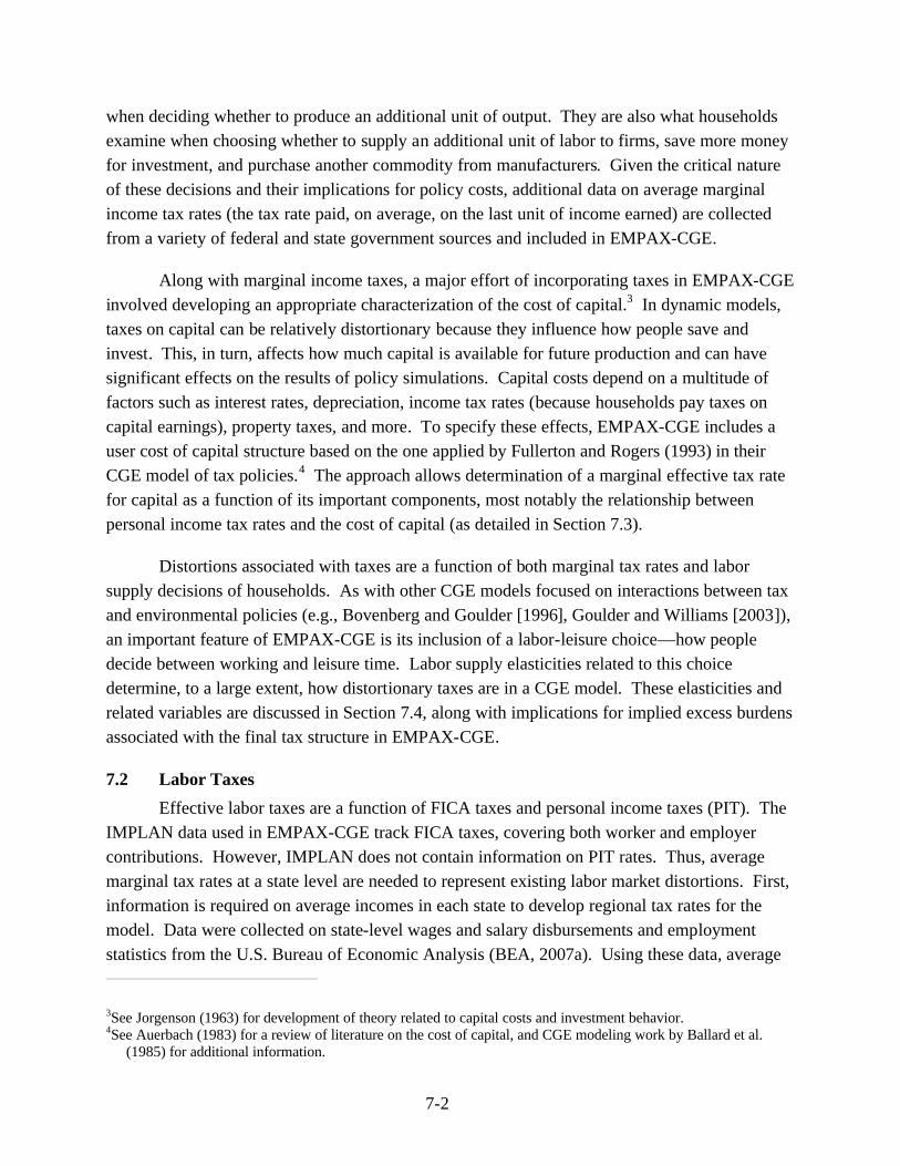
7-2

when deciding whether to produce an additional unit of output. They are also what households examine when choosing whether to supply an additional unit of labor to firms, save more money for investment, and purchase another commodity from manufacturers. Given the critical nature of these decisions and their implications for policy costs, additional data on average marginal income tax rates (the tax rate paid, on average, on the last unit of income earned) are collected from a variety of federal and state government sources and included in EMPAX-CGE.

Along with marginal income taxes, a major effort of incorporating taxes in EMPAX-CGE involved developing an appropriate characterization of the cost of capital.3 In dynamic models, taxes on capital can be relatively distortionary because they influence how people save and invest. This, in turn, affects how much capital is available for future production and can have significant effects on the results of policy simulations. Capital costs depend on a multitude of factors such as interest rates, depreciation, income tax rates (because households pay taxes on capital earnings), property taxes, and more. To specify these effects, EMPAX-CGE includes a user cost of capital structure based on the one applied by Fullerton and Rogers (1993) in their CGE model of tax policies.4 The approach allows determination of a marginal effective tax rate for capital as a function of its important components, most notably the relationship between personal income tax rates and the cost of capital (as detailed in Section 7.3).

Distortions associated with taxes are a function of both marginal tax rates and labor supply decisions of households. As with other CGE models focused on interactions between tax and environmental policies (e.g., Bovenberg and Goulder [1996], Goulder and Williams [2003]), an important feature of EMPAX-CGE is its inclusion of a labor-leisure choice—how people decide between working and leisure time. Labor supply elasticities related to this choice determine, to a large extent, how distortionary taxes are in a CGE model. These elasticities and related variables are discussed in Section 7.4, along with implications for implied excess burdens associated with the final tax structure in EMPAX-CGE.

7.2 Labor Taxes Effective labor taxes are a function of FICA taxes and personal income taxes (PIT). The

IMPLAN data used in EMPAX-CGE track FICA taxes, covering both worker and employer contributions. However, IMPLAN does not contain information on PIT rates. Thus, average marginal tax rates at a state level are needed to represent existing labor market distortions. First, information is required on average incomes in each state to develop regional tax rates for the model. Data were collected on state-level wages and salary disbursements and employment statistics from the U.S. Bureau of Economic Analysis (BEA, 2007a). Using these data, average

3See Jorgenson (1963) for development of theory related to capital costs and investment behavior. 4See Auerbach (1983) for a review of literature on the cost of capital, and CGE modeling work by Ballard et al.

(1985) for additional information.

7-3

labor income for employees within each state is computed by dividing wage and salary earnings by employment figures. As shown in Table 7-1, the U.S. average value in 2005 was approximately $32,500 and state-level averages ranged from $21,200 (Montana) to $60,400 (District of Columbia).

These average state-level earnings are combined with information from the TAXSIM model at the National Bureau of Economic Research (Feenberg and Coutts, 1993). TAXSIM is a microsimulation model of U.S. federal and state income tax systems. It can be used to estimate the average marginal tax rates needed for CGE analyses of taxes. As shown in Table 7-2, the TAXSIM model distinguishes rates by wage, interest, dividend, and capital-gains income. All four types of tax rates are used in Section 7.3 to calculate capital costs, and the wage tax rate is applied to labor earnings in EMPAX-CGE.

Following Ballard et al. (1985), EMPAX-CGE treats FICA as an ad valorem tax on labor and Social Security benefits as lump-sum transfers to households. Combining FICA taxes from the IMPLAN data with TAXSIM’s average marginal wage tax rate gives a total labor tax rate of approximately 39 percent.5 This is similar to the 40 percent figure often cited in literature and used in CGE models (e.g., Williams [1999], Goulder et al. [1999], Browning [1987]).

As with FICA taxes, EMPAX-CGE follows the approaches of Ballard et al. (1985) and Fullerton and Rogers (1993) related to modeling income taxes for different consumer groups (for EMPAX-CGE simulations that distinguish among household income classes). Income taxes are modeled as linear functions of income for each household, where households have different negative intercepts and a single positive marginal PIT rate. This captures differences in average tax rates and represents the progressive nature of the U.S. tax system, but it does not consider all of the complexities of graduated tax schedules (these are captured as much as possible by inclusion of state-specific PIT rates based on income differences across the country).

7.3 Capital Taxes This section discusses the theoretical motivation and derivation of capital taxes used in

EMPAX-CGE, describes the data sources, and reports the resulting tax rate estimates.

7.3.1 Theoretical Approach A characterization in a CGE model of marginal effective tax rates (METR) on capital

needs to account for features such as

• how corporate tax rates affect the cost of capital,

5Average FICA payments in the IMPLAN data represent an approximately 13 percent tax rate, which takes into account phasing out of employee contributions above certain income levels.

7-4

Table 7-1. Wage and Salary Data by State: 2005

State Wages and Salary

Disbursements ($103) Share of Total Average Per Employee Alabama $69,902,189 1.2% $27,633 Alaska $13,742,435 0.2% $31,895 Arizona $99,828,565 1.8% $31,178 Arkansas $38,259,435 0.7% $24,464 California $736,180,803 13.0% $36,746 Colorado $97,350,123 1.7% $31,608 Connecticut $90,536,002 1.6% $41,346 Delaware $19,715,443 0.3% $36,915 District of Columbia $48,285,943 0.9% $60,442 Florida $302,719,974 5.3% $29,721 Georgia $164,324,254 2.9% $31,406 Hawaii $25,357,599 0.4% $30,233 Idaho $20,297,896 0.4% $23,174 Illinois $263,719,718 4.7% $35,390 Indiana $106,533,476 1.9% $28,868 Iowa $50,337,115 0.9% $25,342 Kansas $47,593,373 0.8% $26,357 Kentucky $64,636,378 1.1% $27,063 Louisiana $66,193,924 1.2% $27,039 Maine $20,608,670 0.4% $24,841 Maryland $119,621,779 2.1% $35,801 Massachusetts $165,051,093 2.9% $39,914 Michigan $183,651,753 3.2% $33,091 Minnesota $112,746,867 2.0% $32,147 Mississippi $35,793,125 0.6% $23,780 Missouri $101,760,161 1.8% $28,294 Montana $13,074,355 0.2% $21,229 Nebraska $31,691,898 0.6% $25,964 Nevada $50,107,960 0.9% $32,583 New Hampshire $26,176,493 0.5% $31,060 New Jersey $201,573,503 3.6% $40,112 New Mexico $28,157,867 0.5% $26,433 New York $452,654,143 8.0% $42,051 North Carolina $149,423,406 2.6% $29,012 North Dakota $10,865,392 0.2% $22,939 Ohio $206,591,362 3.6% $30,300 Oklahoma $50,037,354 0.9% $24,063 Oregon $63,492,374 1.1% $28,424 Pennsylvania $230,550,821 4.1% $32,165 Rhode Island $19,491,289 0.3% $31,882 South Carolina $64,502,276 1.1% $27,109 South Dakota $11,881,595 0.2% $21,906 Tennessee $101,304,199 1.8% $27,821 Texas $407,295,824 7.2% $31,287 Utah $40,060,783 0.7% $26,404 Vermont $10,815,541 0.2% $25,361 Virginia $166,466,705 2.9% $35,013 Washington $125,842,021 2.2% $33,652 West Virginia $22,996,720 0.4% $25,293 Wisconsin $102,031,419 1.8% $28,677 Wyoming $9,187,607 0.2% $25,551 United States $5,661,021,000 100.0% $32,500

Source: U.S. Bureau of Economic Analysis (BEA). 2007a. “Detailed Income and Employment Tables by SIC Industry 1958–2005.” <http://www.bea.gov/bea/regional/spi/default.cfm>. As obtained May 2007.

7-5

Table 7-2. Average Marginal Effective Income Tax Rates by Type and State: 2004

Name Wages Interest Dividends Long-Term Capital Gains Alabama 24.4% 26.5% 32.4% 18.8% Alaska 21.8% 26.2% 25.7% 14.7% Arizona 25.1% 26.3% 27.8% 18.6% Arkansas 24.8% 27.2% 33.4% 17.8% California 29.7% 30.7% 28.2% 23.0% Colorado 27.3% 27.8% 30.2% 19.0% Connecticut 29.2% 29.9% 31.8% 19.5% Delaware 27.5% 28.3% 29.5% 19.7% District of Columbia 32.9% 37.1% 35.6% 24.7% Florida 21.7% 23.5% 25.1% 14.6% Georgia 27.2% 29.2% 31.5% 20.1% Hawaii 26.6% 29.6% 31.6% 22.5% Idaho 25.5% 27.4% 30.4% 20.4% Illinois 25.6% 26.8% 29.8% 17.4% Indiana 23.7% 24.2% 28.4% 17.9% Iowa 25.5% 25.5% 28.9% 21.5% Kansas 27.0% 24.9% 28.0% 20.2% Kentucky 25.4% 27.9% 33.7% 19.2% Louisiana 24.0% 26.0% 29.5% 18.6% Maine 26.4% 27.9% 32.3% 22.8% Maryland 27.6% 27.9% 30.7% 19.6% Massachusetts 29.3% 29.6% 31.5% 19.5% Michigan 25.3% 25.7% 27.7% 18.3% Minnesota 27.8% 29.6% 32.7% 21.8% Mississippi 23.3% 22.7% 26.5% 18.0% Missouri 25.8% 27.8% 28.5% 19.9% Montana 23.5% 22.2% 26.3% 18.5% Nebraska 26.1% 26.7% 23.0% 19.9% Nevada 22.5% 26.2% 27.5% 15.0% New Hampshire 23.0% 28.6% 28.5% 15.6% New Jersey 29.1% 29.3% 31.0% 20.9% New Mexico 26.4% 30.3% 29.2% 19.2% New York 29.7% 30.1% 32.4% 21.9% North Carolina 27.5% 29.9% 32.0% 21.1% North Dakota 25.4% 26.8% 30.3% 17.2% Ohio 26.1% 27.2% 30.0% 21.1% Oklahoma 26.3% 26.7% 33.8% 20.1% Oregon 29.6% 28.0% 29.2% 22.2% Pennsylvania 25.3% 25.2% 28.4% 17.5% Rhode Island 27.9% 30.2% 29.7% 23.1% South Carolina 25.9% 28.5% 28.9% 17.8% South Dakota 19.0% 23.9% 24.6% 12.7% Tennessee 20.9% 26.9% 30.0% 14.3% Texas 22.5% 24.1% 26.5% 14.9% Utah 25.4% 29.0% 30.7% 20.8% Vermont 26.4% 24.0% 27.7% 18.3% Virginia 28.3% 28.7% 30.2% 20.3% Washington 22.2% 22.6% 23.5% 14.7% West Virginia 24.3% 23.4% 25.5% 20.0% Wisconsin 25.5% 26.3% 25.3% 14.6% Wyoming 17.9% 20.7% 22.6% 12.5% Weighted Average 25.6% 27.1% 29.2% 18.9%

Source: NBER TAXSIM Model at <http://www.nber.org/~taxsim/> (Feenberg and Coutts, 1993).

7-6

• how PIT paid on capital earnings influence capital costs, • how economic depreciation of capital assets (which depends on asset type) alters costs,

• how corporate structures in different industries shape treatment of capital taxes, and • how capital taxes vary across industries as a result of these interactions.

EMPAX-CGE determines effective capital tax rates by applying the user cost of capital methodology. The theoretical basis for this approach has a long history (see Auerbach [1983] for a review of the method) and has been used in applied general equilibrium models by other researchers such as Fullerton and Rogers (Who Bears the Lifetime Tax Burden? [1993]), subsequently referred to as FR. The FR documentation of how capital taxes were incorporated into their CGE model is relatively unique in its level of detail, both in terms of calculations and the associated data sources and parameter estimates. For these reasons, EMPAX-CGE uses a similar approach, although data used in the calculations have been updated where feasible.

Effective capital costs reflect interactions among a number of variables such as statutory corporate tax rates, PIT on capital earnings, effects of incorporation levels on tax payments, property taxes, and differential tax and depreciation treatments for various types of financial assets. One reason for adopting the FR approach is that it makes these interactions explicit (including relationships with the most implications for model results, i.e., between PIT and capital costs). Tables 7-3 and 7-4 define parameters used in the computations, followed by a discussion of the relevant equations.

For corporations, the cost of financing is a function of interest payments on debt, costs of retained earnings, and costs of new shares.6 As a weighted average across financial instruments, the overall corporate discount rate can thus be expressed as

rc = cdrd + crerre + cnsrns (7.1)

and the noncorporate discount rate can be expressed as

rnc = ndrd + nere. (7.2)

Arbitrage conditions among these rates of return will ensure that they are all equal on a net-of-tax basis, which implies that capital costs can be calculated from the net real return to holding debt [r = i(1 – td) – p] and leads to the following calculations. Because debt financing charges are deductible at the statutory corporate tax rate, firms pay the equivalent of the nominal

6Following FR assumptions, EMPAX-CGE assumes that industries have fixed financial structures.

7-7

Table 7-3. Parameter Definitions (following FR notation)

Parameter Description kcρ Corporate sector gross-of-tax capital costs of type k

kncρ Noncorporate sector gross-of-tax capital costs of type k

i Nominal interest rate rc Corporate sector discount rate (weighted average) rnc Noncorporate sector discount rate (weighted average) rd Discount rate on debt financing rre Discount rate on retained earnings rns Discount rate on new shares re Discount rate on equity wk Property tax rate on capital of type k dk Economic depreciation rate of capital of type k

kcz Present value of depreciation allowance for corporate capital of type k

kncz Present value of depreciation allowance for noncorp capital of type k

Table 7-4. Exogenous Variable Values (following FR notation)

Variable Description Value Source

r Real interest rate 0.05 MIT EPPA model

p Inflation rate 0.03 AEO 2007 (Table 19)

uf Statutory federal corporate tax rate 0.35 IRS Publication 542

us Statutory state corporate tax rates ~0.06 See Table 7-5

u Statutory corporate tax rate ~0.39 See Table 7-8

tPIT Personal income tax rate ~0.29 See Table 7-2

td Income tax rate on interest income (debt financing) ~0.28 See Table 7-2

t re Income tax rate on accrued capital gains (retained earnings) ~0.05 FR and Table 7-2

tns Income tax rate on dividend income (new shares) ~0.28 See Table 7-2

tnc Income tax rate on noncorporate income (or PIT) ~0.29 See Table 7-2

cd Proportion of corporate investment financed by debt 0.34 FR (Table 3-17)

cre Proportion of corporate investment financed by retained earnings 0.33 FR (Table 3-17)

cns Proportion of corporate investment financed by new shares 0.33 FR (Table 3-17)

nd Proportion of noncorporate investment financed by debt 0.34 FR (Table 3-17)

ne Proportion of noncorporate investment financed by retained earnings 0.67 FR (Table 3-17)

7-8

interest rate excluding the statutory rate [rd = i(1 – u)]. For retained earnings, the nominal net return is the corporation’s discount rate, which is a function of taxes paid on debt and the tax rate applied to retained earnings [rre = i(1 – td)/(1 – t re)]. Similarly, the nominal net return for new shares is a function of taxes paid on debt and on dividend earnings [rns = i(1 – td)/(1 – tns)]. Eq. (7.3) presents these three components of the corporate discount rate, weighted by the shares of each in overall corporate financing:

( )[ ] ( ) ( )[ ]

−−+−−+−= )/()(ic /ic uicr nsdnsredredc ττττ 11111 . (7.3)

For firms with a noncorporate structure, interest payments are deductible at the personal income rate applied to equity earnings. Equity returns must equal the return to holding debt because of arbitrage conditions. Eq. (7.4) give these two components of the noncorporate discount rate, which are weighted by the shares of each in overall noncorporate financing:

( )[ ] ( )[ ]dencdnc ininr ττ −+−= 11 . (7.4)

Using the arbitrage condition to determine the real return to capital, r, and simplifying the FR equations by assuming that the PIT is applied to equity returns of noncorporate firms, implies that Eqs. (7.3) and (7.4) can be expressed as7

( )[ ] ( )[ ] ( )[ ]nsnsrerePITdc rcrcurcr τπτπτπ −++−++−−+= 1/)( 1/)( 1))1/()(( (7.5)

[ ] [ ])(n )1/()1)(( πττπ ++−−+= rrnr edPITdnc . (7.6)

After these real returns to capital have been determined, they can be incorporated into an expression of a firm’s profit-maximization decision to determine gross-of-tax costs of capital, following the methodology of Hall and Jorgenson (1967) as described in Fullerton and Lyon (1988) and Fullerton and Rogers (1993). Eqs. (7.7) and (7.8), adapted from FR,8 illustrate these calculations for each type of capital asset, k (equipment, structures, inventories, land, and intangibles such as knowledge). The capital costs are expressed as functions of real returns, inflation, depreciation, PIT, the present value of depreciation allowances (z, which is equal to allowances divided by allowances plus real net returns), and property taxes:

7t re is assumed to be equal to one quarter of the long-term capital gains rate, following Fullerton and Rogers (1993). This reflects the fact that taxes on capital gains can be postponed by not realizing the gains until a future date, thereby lowering the effective tax rate.

8The original FR equations included discounts for investment tax credits that have since been phased out.

7-9

( ) kkkc

kckc uz

ur

δωδπ

ρ −+−−

+−= 1

1 (7.7)

( ) kkkncPIT

PIT

kncknc zr

δωττ

δπρ −+−

−+−

= 11

(7.8)

METRs for capital can then be calculated for each asset class and corporate structure as the difference between the gross-of-tax capital cost (?) minus the net-of-tax cost (r) divided by the gross-of-tax cost. These METR summarize the effects of all taxes applied to capital and characterize how changes in components of METR will affect the cost of capital. Using the data discussed below, EMPAX-CGE develops a weighted average of METR for each industry across all asset types and firm structures, based on the industry’s share of corporate and noncorporate assets and associated types of capital.

7.3.2 Data and Estimated Capital Tax Rates One of the motivations for choosing the approach to estimating capital taxes used by

Fullerton and Rogers (1993) is that they provide detailed information on their parameter estimates and data sources. Where feasible, the parameters, and sources used to develop capital stock estimates underlying user cost of capital calculations, have been updated to the year 2005, consistent with the base year of the IMPLAN database.

Table 7-5 shows state-specific statutory corporate tax rates. These are combined with the top bracket, federal statutory rate of 35 percent to determine regional corporate tax rates (see Table 7-8). Although there may be differences between the location of capital earnings shown in the IMPLAN state-level data and the location where corporate taxes are assessed, these differences are assumed away at the regional level used in EMPAX-CGE.

Along with updating statutory corporate tax rates, the data sources used by EMPAX-CGE to calculate capital assets by industry are based on year 2004 information where possible. As illustrated in Section 7.3, the user cost-of-capital equations require data on five types of assets (equipment, structures, inventory, land, and intangibles) owned by two different types of firms (corporate and noncorporate).

Data on equipment and structures owned by industries are available from the U.S. Bureau of Economic Analysis (BEA, 2004b). However, these data do not distinguish asset values by corporate and noncorporate organizations. For this, BEA data that separate out legal organization forms by broad industry category are employed (see Table 7-6).

7-10

Table 7-5. Corporate Marginal Tax Rates by State: 2005a

Name State Corporate Alabama 6.50% Alaska 9.40% Arizona 6.97% Arkansas 6.50% California 8.84% Colorado 4.63% Connecticut 7.50% Delaware 8.70% District of Columbia 9.98% Florida 5.50% Georgia 6.00% Hawaii 6.40% Idaho 7.60% Illinois 7.30% Indiana 8.50% Iowa 12.00% Kansas 4.00% Kentucky 7.00% Louisiana 8.00% Maine 8.93% Maryland 7.00% Massachusetts 9.50% Michigan 1.90% Minnesota 9.80% Mississippi 5.00% Missouri 6.25% Montana 6.75% Nebraska 7.81% Nevada 0.00% New Hampshire 9.25% New Jersey 9.00% New Mexico 7.60% New York 7.50% North Carolina 6.90% North Dakota 7.00% Ohio 8.50% Oklahoma 6.00% Oregon 6.60% Pennsylvania 9.99% Rhode Island 9.00% South Carolina 5.00% South Dakota 0.00% Tennessee 6.50% Texas 4.50% Utah 5.00% Vermont 9.75% Virginia 6.00% Washington 0.00% West Virginia 9.00% Wisconsin 7.90% Wyoming 0.00%

a The majority of states have only one tax bracket for corporations; however, some states have multiple brackets. In these cases, consistent with Fullerton (1987), EMPAX-CGE uses the top bracket in its calculations.

Source: The Tax Foundation. State Corporate Income Tax Rates. As of December 31, 2005.

7-11

Table 7-6. Equipment and Structures Assets: Corporate and Noncorporate Sectors

Asset Type Corporate Noncorporate

Farms

Equipment and software 11% 89%

Structures 7% 93%

Manufacturing


Structures 98% 2%

Nonfarm nonmanufacturing


Structures 69% 31%

Source: U.S. Bureau of Economic Analysis (BEA). 2004c. “Current-Cost Net Stock of Nonresidential Fixed Assets by Industry Group and Legal Form of Organization, Table 4-1.” <http://www.bea.doc.gov/bea/dn/faweb/AllFATables.asp>. As obtained January 2004.

Data on inventories and land come from two government sources. The U.S. Census Bureau publishes asset data for inventory and land for selected mining and manufacturing industries in the Quarterly Manufacturing Reports (U.S. Bureau of the Census, 2001). Similarly, the U.S. Department of Agricultural estimates land assets in the agricultural sector in the Agricultural Economics and Land Ownership Survey (USDA, 2000). For the majority of the mining and manufacturing data, asset values are distinguished by corporate and noncorporate sectors using the Federal Reserve Board’s Flow of Funds Accounts (see Table 7-7). In cases where updated information could not be identified, data from Fullerton and Rogers (1993) were used to estimate asset distributions.

The final category of assets, intangibles, is established using the methodology described in Fullerton and Lyon (1988). Intangible capital (i.e., knowledge or information) requires investment by firms but is treated differently than other types of assets (in part because there is no tangible asset to measure). The kinds of investments used to develop intangible capital include advertising expenditures, research and development (R&D), and expenses related to training and customer relations. Unlike other assets, these investments are usually deducted from business income immediately, rather than being depreciated over time. This preferential tax treatment has implications for capital tax rates that are accounted for by the user cost of capital approach.

7-12

Table 7-7. Inventory and Land Assets: Corporate and Noncorporate Sectors

Asset Type Corporate Noncorporate

Land 70% 30% Inventory 75% 25%

Source: Federal Reserve Board. 2004. Flow of Funds Accounts of the United States, Coded Tables for Z.1 Release. Tables B.102 and B.103. <http://www.federalreserve.gov/releases/Z1/20040115/Coded/coded.pdf>. As obtained January 2004.

Following Fullerton and Lyon (1988), intangible capital stocks are assumed to comprise the depreciated present values of advertising and R&D expenditures. The U.S. Internal Revenue Service publishes flows of advertising deductions by industry (U.S. IRS, 1995–2001). Implied capital stocks associated with these flows are computed using data for the period 1994–2000, based on an annual depreciation rate of 33 percent. Asset values connected to R&D expenditures are taken from the National Science Foundation’s (NSF) Industrial Research and Development Information System. Data by industry from 1980 to 2000 (NSF, 2001a and 2001b) are employed to estimate capital stock values using an annual depreciation rate of 15 percent. In the absence of other data, Fullerton and Lyon (1988) data are used to distribute these stocks between corporate and noncorporate sectors.

Following this process, findings on the five types of capital assets by industry are combined with the data developed on personal income and statutory corporate tax rates (see Table 7-8). Information from Fullerton and Rogers (1993) on depreciation and property taxes is also used (see Table 7-9), along with general EMPAX-CGE assumptions about real interest rates (set at 5 percent, following the MIT EPPA model). This collection of data is sufficient to allow calculation of the marginal effective tax rates on capital, based on Eqs. (7.1) to (7.8).

Table 7-8. Regional Tax Rates

Region PIT State Corporate9 Combined State and Federal Corporatea

Northeast 28.3% 6.5% 40.5% South 24.5% 6.1% 39.1% Midwest 25.4% 6.3% 39.5% Plains 23.6% 2.7% 38.2% West 27.2% 6.8% 39.2%

a The total statutory corporate tax rate, based on combined state plus federal corporate tax rates, is calculated according to the method used in Fullerton [1987] as federal (35 percent) + state * (1 – federal).

9Capital earnings in each state from the IMPLAN data are used to weight the corporate tax rates across states within regions.

7-13

Table 7-9. Cost Data by Type of Capital

Capital Type Economic Depreciation Depreciation Allowance Property Tax Rate

Equipment 0.1300 0.3400 0.00574

Structures 0.0300 0.1350 0.00865

Inventories 0.0000 0.0000 0.00574

Land 0.0000 0.0000 0.00865

Intangibles 0.2100 1.0000 0.00000

Source: Fullerton, D., and D. Rogers. 1993. “Who Bears the Lifetime Tax Burden?” Washington, DC: The Brookings Institute, except property taxes from authors’ calculations (see text).

Calculations of average effective property tax rates are based on King and Fullerton (1984), which are updated using NIPA data (U.S. BEA, 2004d) on state and local property tax receipts from year 2000. These data are available as a total figure covering personal and business property taxes (equal to $254 billion). Information from King and Fullerton (1984) on the relative shares of business property taxes in total property taxes, separated into land and structures versus equipment and inventories, is used to apportion this total. Multiplying the shares by total property taxes and then dividing the resulting figure by total capital assets of each type (see Table 7-10) gives the property tax rates shown in Table 7-9.

Table 7-10 presents the results of the estimates of capital assets by industry and associated marginal tax rates for the 40 sectors in the regional static version of EMPAX-CGE. For the dynamic version, weighted average rates across relevant industries are used. Unlike the FR model, EMPAX-CGE does not explicitly track asset and firm types once effective tax rates by industry have been estimated. Consequently, the weighted average METR enters EMPAX as a tax on capital earnings by industry. These estimated METR range from around 25 percent in industries such as computers that depend heavily on R&D assets that can be deducted from business profits immediately to more than 40 percent in sectors such as iron and steel where assets mainly comprise equipment and structures that receive less favorable tax treatment.10

Table 7-11 presents the capital asset and METR findings of Fullerton and Rogers (1993) as a weighted average over corporate and noncorporate structures. A comparison of these data to EMPAX-CGE estimates indicates that effective capital tax rates remain around 40 percent for most industries, although there have been changes in tax laws (i.e., reductions in statutory corporate tax rates—FR uses 49.5 percent—and investment tax credits considered in the FR

10As noted in Fullerton (1987), METR tend to show less variation across industries than average tax rates. Thus, use of METR will imply lower overall distortions from capital taxes in a CGE model than average rates.

7-14

calculations have been eliminated).12 The 40 percent figure is similar to what is typically assumed in CGE modeling of tax distortions (e.g., Goulder et al. [1999]).

7.4 Labor Supply Decisions and Tax Distortions The motivation for including taxes in EMPAX-CGE is to adequately represent how

interactions between the existing tax structure and new policies will alter estimated macroeconomic results. Aside from the specific marginal tax rates included in a CGE model, the parameter with the greatest impact on distortionary effects associated with taxes is the labor-supply elasticity. This elasticity controls how willing households are to substitute between leisure time and supplying labor to businesses. If households are very willing to switch between leisure and work in response to changes in wages, existing labor taxes will have significantly distorted economic behavior from what would have occurred in the absence of the taxes, implying a large excess burden for labor taxes, and the reverse if households are not willing to substitute leisure time for work (and hence consumption goods).

Existing taxes on labor income have two effects on labor supply: a substitution effect—a reduction in the amount of labor available for production because they lower income received by households providing the labor and an income effect—an increase in work effort due to the fact that taxes have lowered overall income levels. Which of these two effects dominates is an empirical question. Russek (1996) reviews relevant literature, which cites estimates for total labor supply elasticities (covering both women and men) ranging between –0.1 and 2.3. Fuchs, Krueger, and Poterba (1998) also review estimated elasticities with similar findings.

The values for labor-supply elasticities most commonly used in CGE models are in the mid-point of the range presented by Russek—typically around 0.4 for compensated elasticities and 0.15 for uncompensated elasticities (e.g., Parry and Bento [2000], Williams [1999], Goulder, Parry, and Burtraw [1997], Bovenberg and Goulder [1996]). Selection of labor-supply elasticities for a CGE model must also take into consideration its implications for measurements of how distorting existing taxes are in the model. These distortions are typically measured in two ways: marginal cost of public funds (MCPF) and

12FR used a 4 percent real interest rate and a 4 percent inflation rate. EMPAX-CGE uses a 5 percent real interest rate and a 3 percent inflation rate so these variables have equivalent effects.

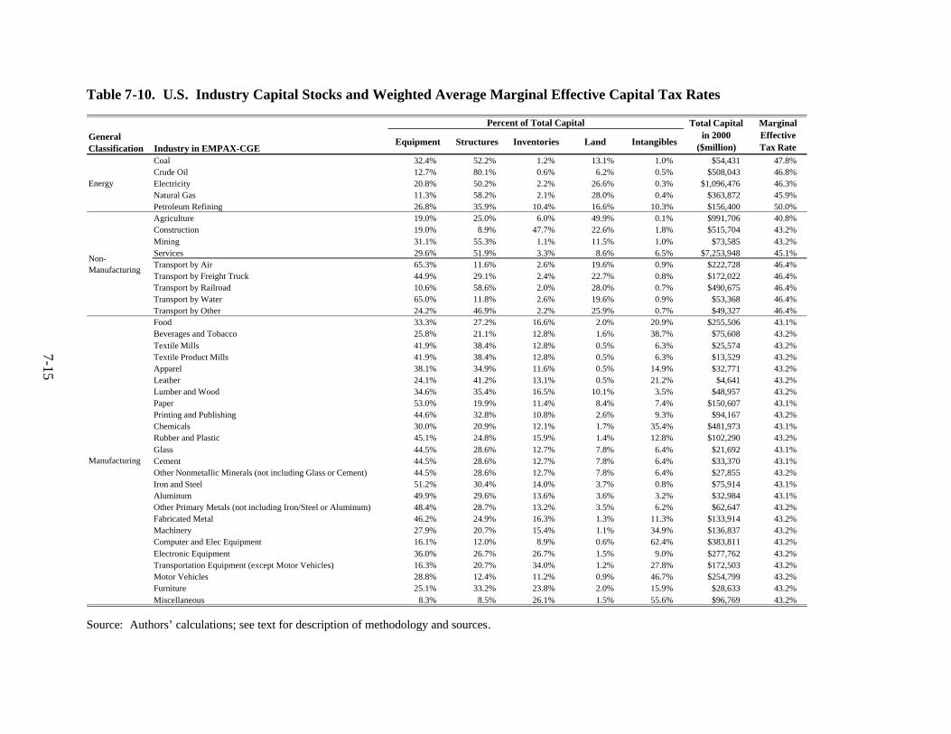
7-15

Table 7-10. U.S. Industry Capital Stocks and Weighted Average Marginal Effective Capital Tax Rates

Equipment Structures Inventories Land Intangibles

Coal 32.4% 52.2% 1.2% 13.1% 1.0% $54,431 47.8% Crude Oil 12.7% 80.1% 0.6% 6.2% 0.5% $508,043 46.8% Electricity 20.8% 50.2% 2.2% 26.6% 0.3% $1,096,476 46.3% Natural Gas 11.3% 58.2% 2.1% 28.0% 0.4% $363,872 45.9% Petroleum Refining 26.8% 35.9% 10.4% 16.6% 10.3% $156,400 50.0% Agriculture 19.0% 25.0% 6.0% 49.9% 0.1% $991,706 40.8% Construction 19.0% 8.9% 47.7% 22.6% 1.8% $515,704 43.2% Mining 31.1% 55.3% 1.1% 11.5% 1.0% $73,585 43.2% Services 29.6% 51.9% 3.3% 8.6% 6.5% $7,253,948 45.1% Transport by Air 65.3% 11.6% 2.6% 19.6% 0.9% $222,728 46.4% Transport by Freight Truck 44.9% 29.1% 2.4% 22.7% 0.8% $172,022 46.4% Transport by Railroad 10.6% 58.6% 2.0% 28.0% 0.7% $490,675 46.4% Transport by Water 65.0% 11.8% 2.6% 19.6% 0.9% $53,368 46.4% Transport by Other 24.2% 46.9% 2.2% 25.9% 0.7% $49,327 46.4% Food 33.3% 27.2% 16.6% 2.0% 20.9% $255,506 43.1% Beverages and Tobacco 25.8% 21.1% 12.8% 1.6% 38.7% $75,608 43.2% Textile Mills 41.9% 38.4% 12.8% 0.5% 6.3% $25,574 43.2% Textile Product Mills 41.9% 38.4% 12.8% 0.5% 6.3% $13,529 43.2% Apparel 38.1% 34.9% 11.6% 0.5% 14.9% $32,771 43.2% Leather 24.1% 41.2% 13.1% 0.5% 21.2% $4,641 43.2% Lumber and Wood 34.6% 35.4% 16.5% 10.1% 3.5% $48,957 43.2% Paper 53.0% 19.9% 11.4% 8.4% 7.4% $150,607 43.1% Printing and Publishing 44.6% 32.8% 10.8% 2.6% 9.3% $94,167 43.2% Chemicals 30.0% 20.9% 12.1% 1.7% 35.4% $481,973 43.1% Rubber and Plastic 45.1% 24.8% 15.9% 1.4% 12.8% $102,290 43.2% Glass 44.5% 28.6% 12.7% 7.8% 6.4% $21,692 43.1% Cement 44.5% 28.6% 12.7% 7.8% 6.4% $33,370 43.1% Other Nonmetallic Minerals (not including Glass or Cement) 44.5% 28.6% 12.7% 7.8% 6.4% $27,855 43.2% Iron and Steel 51.2% 30.4% 14.0% 3.7% 0.8% $75,914 43.1% Aluminum 49.9% 29.6% 13.6% 3.6% 3.2% $32,984 43.1% Other Primary Metals (not including Iron/Steel or Aluminum) 48.4% 28.7% 13.2% 3.5% 6.2% $62,647 43.2% Fabricated Metal 46.2% 24.9% 16.3% 1.3% 11.3% $133,914 43.2% Machinery 27.9% 20.7% 15.4% 1.1% 34.9% $136,837 43.2% Computer and Elec Equipment 16.1% 12.0% 8.9% 0.6% 62.4% $383,811 43.2% Electronic Equipment 36.0% 26.7% 26.7% 1.5% 9.0% $277,762 43.2% Transportation Equipment (except Motor Vehicles) 16.3% 20.7% 34.0% 1.2% 27.8% $172,503 43.2% Motor Vehicles 28.8% 12.4% 11.2% 0.9% 46.7% $254,799 43.2% Furniture 25.1% 33.2% 23.8% 2.0% 15.9% $28,633 43.2% Miscellaneous 8.3% 8.5% 26.1% 1.5% 55.6% $96,769 43.2%

Percent of Total Capital Total Capital in 2000

($million)

Marginal Effective Tax Rate

Energy

Non-Manufacturing

Manufacturing

General Classification Industry in EMPAX-CGE

Source: Authors’ calculations; see text for description of methodology and sources.

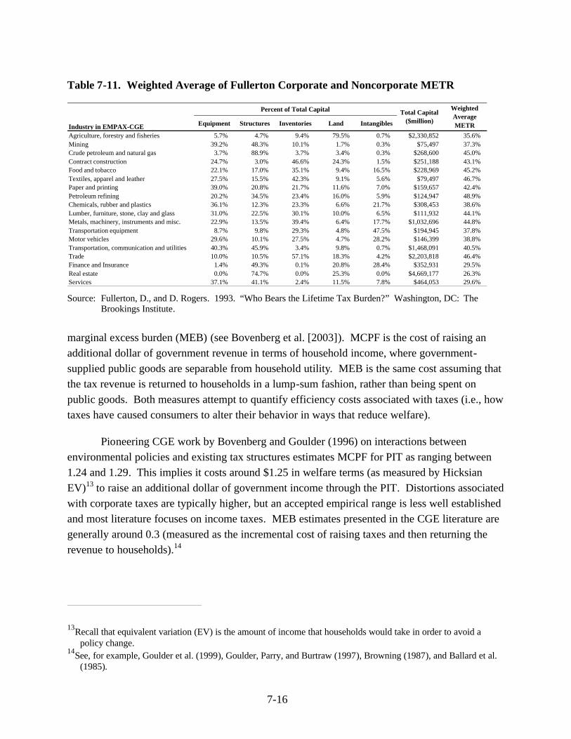
7-16

Table 7-11. Weighted Average of Fullerton Corporate and Noncorporate METR

Equipment Structures Inventories Land Intangibles

Agriculture, forestry and fisheries 5.7% 4.7% 9.4% 79.5% 0.7% $2,330,852 35.6% Mining 39.2% 48.3% 10.1% 1.7% 0.3% $75,497 37.3% Crude petroleum and natural gas 3.7% 88.9% 3.7% 3.4% 0.3% $268,600 45.0% Contract construction 24.7% 3.0% 46.6% 24.3% 1.5% $251,188 43.1% Food and tobacco 22.1% 17.0% 35.1% 9.4% 16.5% $228,969 45.2% Textiles, apparel and leather 27.5% 15.5% 42.3% 9.1% 5.6% $79,497 46.7% Paper and printing 39.0% 20.8% 21.7% 11.6% 7.0% $159,657 42.4% Petroleum refining 20.2% 34.5% 23.4% 16.0% 5.9% $124,947 48.9% Chemicals, rubber and plastics 36.1% 12.3% 23.3% 6.6% 21.7% $308,453 38.6% Lumber, furniture, stone, clay and glass 31.0% 22.5% 30.1% 10.0% 6.5% $111,932 44.1% Metals, machinery, instruments and misc. 22.9% 13.5% 39.4% 6.4% 17.7% $1,032,696 44.8% Transportation equipment 8.7% 9.8% 29.3% 4.8% 47.5% $194,945 37.8% Motor vehicles 29.6% 10.1% 27.5% 4.7% 28.2% $146,399 38.8% Transportation, communication and utilities 40.3% 45.9% 3.4% 9.8% 0.7% $1,468,091 40.5% Trade 10.0% 10.5% 57.1% 18.3% 4.2% $2,203,818 46.4% Finance and Insurance 1.4% 49.3% 0.1% 20.8% 28.4% $352,931 29.5% Real estate 0.0% 74.7% 0.0% 25.3% 0.0% $4,669,177 26.3% Services 37.1% 41.1% 2.4% 11.5% 7.8% $464,053 29.6%

Industry in EMPAX-CGE

Percent of Total Capital Total Capital ($million)

Weighted Average METR

Source: Fullerton, D., and D. Rogers. 1993. “Who Bears the Lifetime Tax Burden?” Washington, DC: The

Brookings Institute.

marginal excess burden (MEB) (see Bovenberg et al. [2003]). MCPF is the cost of raising an additional dollar of government revenue in terms of household income, where government-supplied public goods are separable from household utility. MEB is the same cost assuming that the tax revenue is returned to households in a lump-sum fashion, rather than being spent on public goods. Both measures attempt to quantify efficiency costs associated with taxes (i.e., how taxes have caused consumers to alter their behavior in ways that reduce welfare).

Pioneering CGE work by Bovenberg and Goulder (1996) on interactions between environmental policies and existing tax structures estimates MCPF for PIT as ranging between 1.24 and 1.29. This implies it costs around $1.25 in welfare terms (as measured by Hicksian EV)13 to raise an additional dollar of government income through the PIT. Distortions associated with corporate taxes are typically higher, but an accepted empirical range is less well established and most literature focuses on income taxes. MEB estimates presented in the CGE literature are generally around 0.3 (measured as the incremental cost of raising taxes and then returning the revenue to households).14

13Recall that equivalent variation (EV) is the amount of income that households would take in order to avoid a policy change.

14See, for example, Goulder et al. (1999), Goulder, Parry, and Burtraw (1997), Browning (1987), and Ballard et al. (1985).

7-17

To estimate MEB in EMPAX-CGE, equal-yield constraints on government income have been included in the model. These equations allow a CGE model to replace an existing tax instrument with an alternative approach that raises the same amount of revenue—or maintains a given level of utility. Following Ballard et al. (1985), the equal-yield constraints in EMPAX-CGE are modeled as ensuring equal purchasing power for the government at the new prices prevailing under the alternative tax policy.15

In EMPAX-CGE, the compensated labor-supply elasticity is set at 0.40 and the uncompensated labor-supply elasticity is set at 0.15, based on estimates used in the other CGE models mentioned above. This implies the elasticity between consumption goods and leisure (s cl) equals approximately 0.85. Table 7-12 illustrates the MCPF and MEB associated with these assumptions for several types of taxes. These findings are based on all interactions among economic and energy data, tax rates, CES production functions, and production and consumption elasticities in the current structure of EMPAX-CGE (changes in any of these data or assumptions may alter MCPF and MEB estimates).16

Table 7-12. MCPF and MEB Estimates in the Dynamic Version of EMPAX-CGE

Tax Instrument MCPF MEB

All Taxes 1.23 0.30

Personal Income Taxes 1.24 0.31

Statutory Corporate Taxes 1.31 0.38

aMCPF and MEB calculations are based on model runs with a single household in each region to allow comparison of the results to existing estimates in the literature. As noted in Bovenberg and Goulder, the appropriate equilibrium, at which to measure MCPF is a post-policy equilibrium, so MCPF also depends on the policy in question.

15This avoids the need to specify a utility function for the government and limits the number of utility-maximizing agents in the model (which simplifies results interpretation).

16As noted in Bovenberg and Goulder, the appropriate equilibrium at which to measure MCPF is a post-policy equilibrium, so MCPF also depends on the policy in question.

R-1

REFERENCES

Adkins, L.G., and R.F. Garbaccio. 1999. “A Bibliography of CGE Models Applied to Environmental Issues.” U.S. Environmental Protection Agency, Office of Economy and Environment. Available at <http://www.ksg.harvard.edu/cbg/ptep/cge.bib.2e.pdf>.

Armington, P.S. 1969. “A Theory of Demand for Products Distinguished by Place of Production.” IMF Staff Papers 16:159-178.

Arrow, K.J., and G. Debreu. 1954. “Existence of an Equilibrium for a Competitive Economy.” Econometrica 22:265-290.

Arrow, K.J., and F.H. Hahn. 1971. General Competitive Analysis. San Francisco: Holden-Day.

Auerbach, A.J. 1983. “Corporate Taxation in the United States.” Brookings Papers on Economic Activity 2:451-505.

Babiker, M.H., and T.F. Rutherford. 1997. “Input-Output and General Equilibrium Estimates of Embodied Carbon: A Data Set and Static Framework for Assessment.” University of Colorado at Boulder, Working Paper 97-2.

Babiker, M.H., J.M. Reilly, M. Mayer, R.S. Eckaus, I.S. Wing, and R.C. Hyman. 2001. “The MIT Emissions Prediction and Policy Analysis (EPPA) Model: Revisions, Sensitivities, and Comparisons of Results.” MIT Joint Program on the Science and Policy of Global Change, Report No. 71. Cambridge, MA.

Babiker, M.H., G.E. Metcalf, and J. Reilly. 2002. “Tax Distortions and Global Climate Policy.” MIT Joint Program on the Science and Policy of Global Change, Report No. 85. Cambridge, MA.

Ballard, C.L. 2000. "How Many Hours are in a Simulated Day? The Effects of Time Endowment on the Results of Tax-Policy Simulation Models." Michigan State University, June 28, 2000. This is a revised version of a paper presented at the Conference on Using OLG Models for Policy Analysis, Copenhagen, Denmark, August 13-14, 1999.

Balistreri, E.J., and T.F. Rutherford. 2001. “Dynamic General Equilibrium Analysis at the State Level: Assessing the Economic Implications of the Kyoto Protocol.” Conference Proceedings: Fourth Annual Conference on Global Economic Analysis, vol. II, June 27-29, Purdue University. <http://www.georgetown.edu/faculty/ejb37/Papers/CO2004.pdf>.

Ballard, C.L., D. Fullerton, J.B. Shoven, and J. Whalley. 1985. A General Equilibrium Model for Tax Policy Evaluation. Chicago: University of Chicago Press.

Beach, R.H., and B.M. Depro. “Competitiveness Analyses of Alternative SAMI Strategies.” Prepared for the U.S. Environmental Protection Agency, March 2002.

R-2

Bergman, L. 1988. “Energy Policy Modeling: A Survey of General Equilibrium Approaches.” Journal of Policy Modeling 12(4):671-691.

Bernstein, P.M., W.D. Montgomery, T.F. Rutherford, and G. Yang. 1999. “Effects of Restrictions on International Permit Trading: The MS-MRT Model.” The Energy Journal (Kyoto Special Issue):221-256.

Bovenberg, L.A., and L.H. Goulder. 1996. “Optimal Environmental Taxation in the Presence of Other Taxes: General-Equilibrium Analysis.” American Economic Review 86(4):985-1000.

Bovenberg, L.A., and L.H. Goulder. 2000. “Neutralizing the Adverse Industry Impacts of CO2 Abatement Policies: What Does It Cost?” In Behavioral and Distributional Impacts of Environmental Policies, C. Carraro and G. Metcalf (eds.). Chicago, IL: University of Chicago Press.

Bovenberg, A.L., L.H. Goulder, and D.J. Gurney. 2003. “E? ciency Costs of Meeting Industry-Distributional Constraints under Environmental Permits and Taxes.” Stanford University working paper, <http://www.stanford.edu/~goulder/Bovenberg-Goulder-Gurney%20Paper.pdf>.

Brooke, A., D. Kendrick, A. Meeraus, and R. Raman. 1998. GAMS: A User’s Guide. GAMS Development Corporation. <http://www.gams.com>.

Browning, E.K. 1987. “On the Marginal Welfare Cost of Taxation.” American Economic Review 77:11-23.

Burfisher, M., S. Robinson, and K. Thierfelder. 1994. “Wage Changes in a U.S.-Mexico Free Trade Area: Migration versus Stolper-Samuelson Effects.” In Modeling Trade Policy: Applied General Equilibrium Assessments of North American Free Trade. J. Francois and C. Shiells (eds.). Cambridge: Cambridge University Press.

Burniaux, J.M., G. Nicoletti, and J. Oliveira-Martins. 1992. “GREEN: A Global Model for Quantifying the Cost of Policies to Curb CO2 Emissions.” OECD Economic Studies 19:123-140.

Cass, D. 1965. “Optimum Growth in an Aggregative Model of Capital Accumulation.” Review of Economic Studies 32:233-240.

Conrad, K. 1999. “Computable General Equilibrium Models for Environmental Economics and Policy Analysis,” in: J.C.J.M. van den Bergh (ed.): Handbook of Environmental and Resource Economics, Cheltenham, Edward Elgar, 1061-1087.

Conrad, K. 2001. “Computable General Equilibrium Models in Environmental and Resource Economics,” in: T. Tietenberg and H. Folmer (eds.): The International Yearbook of Environmental and Resource Economics 2002/2003, 66-114.

R-3

Deardorff, A.V., and M. Stern. 1981. “A Disaggregated Model of World Production and Trade: An Estimate of the Impact of the Tokyo Round.” Journal of Policy Modeling 3:127-152.

Despotakis, K.A., and A.C. Fisher. 1988. “Energy in a Regional Economy: A Computable General Equilibrium Model for California.” Journal of Environmental Economics and Management 15(3):313-330.

Edmonds, J., and J. Reilly. 1985. Global Energy: Assessing the Future. New York: Oxford University Press.

Espinoza, J., and V. Kerry Smith. 1995. “Measuring the Environmental Consequences of Trade Policy: A Nonmarket CGE Analysis.” American Journal of Agricultural Economics 77(August 1995):772-777.

Federal Reserve Board. 2004. Flow of Funds Accounts of the United States, Coded Tables for Z.1 Release. Tables B.102 and B.103. <http://www.federalreserve.gov/releases/ Z1/20040115/Coded/coded.pdf>. As obtained January 2004.

Feenberg, D., and E. Coutts. 1993. “An Introduction to the TAXSIM Model.” Journal of Policy Analysis and Management 12(1): 189-194. <http://www.nber.org/~taxsim/>.

Francois, J., and C. Shiells (eds.). 1994. Modeling Trade Policy: Applied General Equilibrium Assessments of North American Free Trade. Cambridge: Cambridge University Press.

Fuchs, V.R., A.B. Krueger, and J.M. Poterba. 1998. “Economists’ Views about Parameters, Values, and Policies: Survey Results in Labor and Public Economics.” Journal of Economic Literature 36:1387-1425.

Fullerton, D. 1987. “The Indexation of Interest, Depreciation, and Capital Gains and Tax Reform in the United States.” Journal of Public Economics 32:25-51.

Fullerton, D., and A. Lyon. 1988. “Tax Neutrality and Intangible Capital.” In Tax Policy and the Economy, vol. 2, Lawrence Summers (ed.), p. 63-88. Cambridge, MA: MIT Press.

Fullerton, D., and G.E. Metcalfe. 2001. “Environmental Controls, Scarcity Rents, and Pre-Existing Distortions.” Journal of Public Economics 80:249-267.

Fullerton, D., and D. Rogers. 1993. “Who Bears the Lifetime Tax Burden?” Washington, DC: The Brookings Institute.

Goulder, L.H. 2000. “Confronting the Adverse Industry Impacts of CO2 Abatement Policies: What Does It Cost?” Resources for the Future: Climate Issues Brief No. 23.

Goulder, L.H., Ian W.H. Parry, R.C. Williams, and D. Burtraw. 1999. “The Cost-Effectiveness of Alternative Instruments for Environmental Protection in a Second-Best Setting.” Journal of Public Economics 72:329-360.

R-4

Goulder, L.H., and R.C. Williams. 2003. “The Substantial Bias from Ignoring General Equilibrium Effects in Estimating Excess Burden, and a Practical Solution.” Journal of Political Economy 111:898-927.

Goulder, L.H., Ian W.H. Parry, and D. Burtraw. 1997. “Revenue-Raising Versus Other Approaches to Environmental Protection: The Critical Significance of Preexisting Tax Distortions.” Rand Journal of Economics 28:708-731.

Hall, R.E., and D.W. Jorgenson. 1967. “Tax Policy and Investment Behavior.” American Economic Review 57:391-414.

Harberger, A.C. 1959. “The Corporate Income Tax: An Empirical Appraisal.” In Tax Revision Compendium, Vol. 1. House Committee on Ways and Means. Washington D.C.: Government Printing Office.

Harberger, A.C. 1962. “The Incidence of the Corporation Income Tax.” Journal of Political Economy 70:215-240.

Harberger, A.C. 1966. “Efficiency Effects of Taxes on Income from Capital.” In Effects of Corporation Income Tax, M. Krzyzaniak (ed.). Detroit: Wayne State University Press.

Harberger, A.C. 1974. Taxation and Welfare. Chicago: University of Chicago Press.

Harrison, G.W., and T.F. Rutherford. 1998. “Burden Sharing, Joint Implementation, and Carbon Coalitions.” In International Environmental Agreements on Climate Change, Amsterdam: Kluwer.

Hazilla, Michael, and Raymond Kopp. 1990. “Social Cost of Environmental Regulations: A General Equilibrium Analysis.” Journal of Political Economy 98(4):853-872.

Ho, M.S., and D.W. Jorgenson. 1998. “Environmental Regulation and U.S. Trade.” In Growth, Volume 2: Energy, the Environment, and Economic Growth, D.W. Jorgenson (ed.). Cambridge, MA: MIT Press.

Industrial Economics, Inc. (IEC). 2001. “Benefits and Costs of the Clean Air Act 1990-2020: Draft Analytical Plan for EPA’s Second Prospective Analysis.” Prepared for the U.S. Environmental Protection Agency, Office of Policy Analysis and Review.

Jacoby, H.D., J.M. Reilly, J.R. McFarland, and S. Paltsev. 2004. “Technology and Technical Change in the MIT EPPA Model.” MIT Joint Program on the Science and Policy of Global Change, Report No. 111. Cambridge, MA. <http://web.mit.edu/globalchange/www/MITJPSPGC_Rpt111.pdf>.

Johansen, Leif. 1960. A Multi-Sectoral Study of Economic Growth. Amsterdam, The

Netherlands: North-Holland.

Jorgenson, D.W. 1963. “Capital Theory and Investment Behavior.” American Economic Review 53(2):247-259.

R-5

Jorgenson, D.W. 1998. Growth, Volume 2: Energy, the Environment, and Economic Growth. Cambridge, MA: MIT Press.

Jorgenson, D.W., and P.J. Wilcoxen. 1990a. “Environmental Regulation and U.S. Economic Growth.” Rand Journal of Economics 21(2):314-340.

Jorgenson, D.W., and P.J. Wilcoxen. 1990b. “Intertemporal General Equilibrium Modeling of U.S. Environmental Regulation.” Journal of Policy Modeling 12(4):715-744.

Jorgenson, D.W., and P.J. Wilcoxen. 1993a. “The Economic Impact of the Clean Air Act Amendments of 1990.” The Energy Journal 14(1):159-182.

Jorgenson, D.W., and P.J. Wilcoxen. 1993b. “Reducing U.S. Carbon Dioxide Emissions: An Econometric General Equilibrium Assessment.” Resource and Energy Economics 15(1):7-25.

Jorgenson, D.W., and P.J. Wilcoxen. 1993c. “Reducing U.S. Carbon Dioxide Emissions: An Assessment of Alternative Instruments.” Journal of Policy Modeling 15(5&6):491-520.

Jorgenson, D.W., and P.J. Wilcoxen. 1993d. “Energy, the Environment, and Economic Growth.” In Handbook of Natural Resource and Energy Economics, Volume 3, A.V. Kneese and J.L. Sweeney (eds.). New York: Elsevier Sciences.

Jorgenson, D.W., and P.J. Wilcoxen. 1997. “Fundamental U.S. Tax Reform and Energy Markets.” The Energy Journal 18(3):1-30.

Jorgenson, D.W., and P.J. Wilcoxen. 1998. “The Economic Impact of the Clean Air Act Amendments of 1990.” In Growth. Volume 2: Energy, the Environment, and Economic Growth, D.W. Jorgenson (ed.). Cambridge, MA: MIT Press.

King, M.A., and D. Fullerton. 1984. The Taxation of Income from Capital. Chicago, IL: University of Chicago Press.

King, B. 1985. “What is a SAM?” Pyatt, G. and J. I. Round (eds.), Social Accounting Matrices: A Basis for Planning. Washington D. C.: The World Bank.

Koopmans, T.C. 1965. “On the Concept of Optimal Economic Growth.” In The Econometric Approach to Development Planning. Amsterdam: North Holland.

Lau, M., A. Pahlke, and T. Rutherford. 2000. “Approximating Infinite-Horizon Models in a Complementarity Format: A Primer in Dynamic General Equilibrium Analysis.” University of Colorado working paper.

Leontief, W.W. 1936. “Quantitative Input-Output Relations in the Economic System of the United States.” The Review of Economics and Statistics 18:105-25.

Leontief, W.W. 1951. The Structure of the American Economy, 1919-1939, 2nd ed. New York: Oxford University Press.

R-6

Leontief, W.W. (ed.). 1953. Studies in the Structure of the American Economy. New York: Oxford University Press.

Manne, A., and R. Richels. March 1997. “On Stabilizing CO2 Concentrations: Cost-Effective Emission Reduction Strategies.” Paper presented at the IPCC Asia-Pacific Workshop on Integrated Assessment Models, the United Nations University, Tokyo, Japan.

Martin, W., and L.A. Winters. 1996. The Uruguay Round and the Developing Countries. Cambridge: Cambridge University Press.

McKibbin, W.J., M.T. Ross, R. Shackleton, and P.J. Wilcoxen. 1999. “Emissions Trading, Capital Flows, and the Kyoto Protocol.” The Energy Journal (Kyoto Special Issue):287-333.

Nainar, S.M.K. 1989. “Bootstrapping for Consistent Standard Errors for Translog Price Elasticities.” Energy Economics 11:319-322.

National Science Foundation (NSF). 2001a. “Company and Other Non-Federal Funds for Industrial R&D Performance in the U.S., by Industry and Size of Company: 1997–2000.” Table A-7. <http://www.nsf.gov/sbe/srs/iris/start.htm>. Last updated September 2001.

National Science Foundation (NSF). 2001b. “Company and Other (Except Federal) Funds for Industrial R&D Performance, by Industry and by Size of Company: 1953–98.” Table H-25. <http://www.nsf.gov/sbe/srs/iris/start.htm>. Last updated September 2001.

Nestor, D.V., and C.A. Pasurka. 1995. “Environment-Economic Accounting and Indicators of the Economic Importance of Environmental Protection Activities.” Review of Income and Wealth 41(3):265-287.

Nguyen, H.V. 1987. “Energy Elasticities Under Divisia and Btu Aggregation.” Energy Economics 9:210-214.

Paltsev, S., J.M. Reilly, H.D. Jacoby, A.D. Ellerman, and K.H. Tay. 2003. “Emissions Trading to Reduce Greenhouse Gas Emissions in the United States: The McCain-Lieberman Proposal.” MIT Joint Program on the Science and Policy of Global Change, Report No. 97. <http://web.mit.edu/globalchange/www/MITJPSPGC_Rpt97.pdf>.

Paltsev, S., J.M. Reilly, H.D. Jacoby, R.S. Eckaus, J. McFarland, M. Sarofim, M. Asadoorian, and M. Babiker. 2005. “The MIT Emissions Prediction and Policy Analysis (EPPA) Model: Version 4.” MIT Joint Program on the Science and Policy of Global Change, Report No. 125. Cambridge, MA. <http://web.mit.edu/globalchange/www/eppa.html>.

Parry, Ian W.H. 1997. “Environmental Taxes and Quotas in the Presence of Distorting Taxes in Factor Markets.” Resource and Energy Economics 19:203-220.

Parry, Ian W.H. 1999. “Agricultural Policies in the Presence of Distorting Taxes.” American Journal of Agricultural Economics 81:212-230.

R-7

Parry, Ian W.H. and A.M. Bento. 2000. “Tax Deductions, Environmental Policy, and the ‘Double Dividend’ Hypothesis.” Journal of Environmental Economics and Management 39:67-96.

Perroni, C. and R.M. Wigle. 1994. “International Trade and Environmental Quality: How Important are the Linkages?” Canadian Journal of Economics 27(3):551-567.

Pindyck, R.S. 1979. “Interfuel Substitution and the Industrial Demand for Energy: An International Comparison.” Review of Economics and Statistics 61:169-179.

Ramsey, F.P. 1928. “A Mathematical Theory of Saving.” Economic Journal 38:543-559.

Robinson, S., M. Burfisher, R. Hinojosa, and K. Thierfelder. 1991. “Agriculture in a U.S.-Mexico Free Trade Agreement: A Computable General Equilibrium Model with Migration and Farm Programs.” Giannini Foundation Working Paper No. 617.

Rose, A., and G. Oladosu. 2002. “Greenhouse Gas Reduction Policy in the United States: Identifying Winners and Losers in an Expanded Permit Trading System.” Energy Journal 23(1):1-18.

Russek, F.S. 1996. “Labor Supply and Taxes.” Congressional Budget Office working paper. <ftp://ftp.cbo.gov/33xx/doc3372/labormkts.pdf>.

Rutherford, T.F. 1999. “Applied General Equilibrium Modeling with MPSGE as a GAMS Subsystem: An Overview of the Modeling Framework and Syntax.” Computational Economics 14(1):1-46.

Rutherford, T.F. 2004. “Tools for Building National Economic Models Using State-Level IMPLAN Social Accounts.” University of Colorado Web site <http://debreu.colorado.edu/implan98.htm>.

Rutherford, T.F., and S.V. Paltsev. 2000. “GTAP-Energy in GAMS: The Dataset and Static Model.” University of Colorado at Boulder, Working Paper 00-2.

Schafer, D., and C. Stahmer. 1989. “Input-Output Model for the Analysis of Environmental Protection Activities.” Economic Systems Research 1(2):203-228.

Shoven, J.B., and J. Whalley. 1972. “A General Equilibrium Calculation of the Effects of Differential Taxation of Income from Capital in the U.S.” Journal of Public Economics 1:281-322.

Shoven, J.B., and J. Whalley. 1973. “General Equilibrium with Taxes: A Computation Procedure and an Existence Proof.” Review of Economic Studies 40:475-490.

Shoven, J.B., and J. Whalley. 1992. Applying General Equilibrium. Cambridge: Cambridge University Press.

R-8

Smith, V.K., H. Sieg, H.S. Banzhaf, and R. Walsh. 2003. “General Equilibrium Benefits for Environmental Improvements: Projected Ozone Reductions under EPA’s Prospective Analysis for the Los Angeles Air Basin.” Working Paper.

Summers, L.H. 1981. “Taxation and Corporate Investment: A q-Theory Approach.” Brookings Papers on Economic Activity: 67-127.

The Tax Foundation. 2006a. State General Sales and Use Tax Rates. <http://www.taxfoundation.org/taxdata>. As of December 31, 2005.

The Tax Foundation. 2006b. State Corporate Income Tax Rates. <http://www.taxfoundation.org/taxdata>. As of December 31, 2005.

The Tax Foundation. 2006c. State Gasoline Tax Rates. <http://www.taxfoundation.org/taxdata>. As of December 31, 2005.

U.S. Bureau of Economic Analysis (BEA). 2007a. “Detailed Income and Employment Tables by SIC Industry 1958–2005.” <http://www.bea.gov/bea/regional/spi/default.cfm>. As obtained May 2007.

U.S. Bureau of Economic Analysis (BEA). 2007b. “Detailed Estimates for Private Nonresidential Fixed Assets by Detailed Industry and by Detailed Asset Type, Current Cost Net Stocks: 1947-2005.” <http://www.bea.doc.gov/bea/dn/faweb/ Details/Index.html>. As obtained May 2007.

U.S. Bureau of Economic Analysis (BEA). 2004c. “Current-Cost Net Stock of Nonresidential Fixed Assets by Industry Group and Legal Form of Organization, Table 4-1.” <http://www.bea.doc.gov/bea/dn/faweb/AllFATables.asp>. As obtained January 2004.

U.S. Bureau of Economic Analysis (BEA). 2004d. “State and Local Government Current Receipts and Expenditures, Table 3-3.” <http://www.bea.doc.gov/bea/dn/ nipaweb/Index.asp>. As obtained January 2004.

U.S. Bureau of Labor Statistics (BLS). 2004. Consumer Expenditure Survey. <http://www.bls.gov/cex/home.htm>.

U.S. Census Bureau. 2001. Quarterly Financial Report for Manufacturing, Mining, and Trade Corporations. Third Quarter 2001, Series QFR/01-Q3. Washington, DC: U.S. Government Printing Office.

U.S. Census Bureau. 2004. Decennial Census and Population Surveys. <http://www.census.gov/population/www/index.html>.

U.S. Department of Agriculture (USDA). 2000. “1999 Agriculture Economics and Land Ownership Survey, Table 72.” <http://www.nass.usda.gov/census/census97/ aelos/aelos.htm>. As obtained January 2004.

R-9

U.S. Energy Information Administration (EIA) at Department of Energy (DOE). Commercial Buildings Energy Consumption Survey. <http://www.eia.doe.gov/emeu/cbecs/ce951b.html>.

U.S. Energy Information Administration (EIA) at Department of Energy (DOE). International Energy Annual 2004. <http://www.eia.doe.gov/iea/>.

U.S. Energy Information Administration (EIA) at Department of Energy (DOE). International Energy Price Information. <http://www.eia.doe.gov/emeu/international/prices.html>.

U.S. Energy Information Administration (EIA) at Department of Energy (DOE). Manufacturing Energy Consumption Survey 2002. <http://www.eia.doe.gov/emeu/mecs/contents.html>.

U.S. Energy Information Administration (EIA) at Department of Energy (DOE). 2001. Natural Gas Transportation: Infrastructure Issues and Operations Trends. <http://www.eia.doe.gov/pub/oil_gas/natural_gas/analysis_publications/natural_gas_infrastructure_issue/pdf/nginfrais.pdf>.

U.S. Energy Information Administration (EIA) at Department of Energy (DOE). 2004. Coal Transportation: Rates and Trends in the United States, 1979-2001. <http://www.eia.doe.gov/cneaf/coal/page/trans/ratesntrends.html>.

U.S. Energy Information Administration (EIA) at Department of Energy (DOE). 2005a. Coal Distribution Report 2004. <http://www.eia.doe.gov/cneaf/coal/page/coaldistrib/coal_distributions.html>.

U.S. Energy Information Administration (EIA) at Department of Energy (DOE). 2005b. Annual Energy Review 2005. DOE/EIA-0384. <http://www.eia.doe.gov/emeu/aer/contents.html>.

U.S. Energy Information Administration (EIA) at Department of Energy (DOE). 2005c. International Energy Outlook 2004. DOE/EIA-0484. <http://www.eia.doe.gov/oiaf/ieo/index.html>.

U.S. Energy Information Administration (EIA) at Department of Energy (DOE). 2007. Annual Energy Outlook 2007. DOE/EIA-0383. <http://www.eia.doe.gov/oiaf/archive/aeo07/index.html>.

U.S. Energy Information Administration (EIA) at Department of Energy (DOE). 2006a. Assumptions to the Annual Energy Outlook 2006. DOE/EIA-0445. <http://www.eia.doe.gov/oiaf/aeo/assumption/index.html>.

U.S. Energy Information Administration (EIA) at Department of Energy (DOE). 2006b. Annual Coal Report 2005. DOE/EIA-0584. <http://www.eia.doe.gov/cneaf/coal/page/acr/acr_sum.html>.

R-10

U.S. Energy Information Administration (EIA) at Department of Energy (DOE). 2006e. Petroleum Supply Annual 2005, Volume 1. DOE/EIA-0340/1. <http://www.eia.doe.gov/oil_gas/petroleum/data_publications/petroleum_supply_annual/psa_volume1/psa_volume1.html>.

U.S. Energy Information Administration (EIA) at Department of Energy (DOE). 2006d. Natural Gas Annual 2005. DOE/EIA-0131. <http://www.eia.doe.gov/oil_gas/natural_gas/data_publications/natural_gas_annual/nga.html>.

U.S. Energy Information Administration (EIA) at Department of Energy (DOE). 2006e. Electric Power Annual 2005. DOE/EIA-0348. <http://www.eia.doe.gov/cneaf/electricity/epa/epa_sum.html>.

U.S. Energy Information Administration (EIA) at Department of Energy (DOE). 2006f. Renewable Energy Annual 2004. DOE/EIA-0603. <http://www.eia.doe.gov/cneaf/solar.renewables/page/rea_data/rea_sum.html>.

U.S. Energy Information Administration (EIA) at Department of Energy (DOE). 2006g. Refinery Capacity Report 2006. <http://www.eia.doe.gov/oil_gas/petroleum/data_publications/refinery_capacity_data/refcapacity.html>.

U.S. Energy Information Administration (EIA) at Department of Energy (DOE). 2006h. State Energy Consumption, Price, and Expenditure Estimates 2003. <http://www.eia.doe.gov/emeu/states/_seds.html>.

U.S. Environmental Protection Agency (EPA). 1995a. The U.S. Environmental Protection Industry: A Proposed Framework for Assessment. Office of Policy, Planning, and Evaluation, EPA 230-R-95-011.

U.S. Environmental Protection Agency (EPA). 1995b. The U.S. Environmental Protection Industry: The Technical Document. Office of Policy, Planning, and Evaluation, EPA 230-R-95-012.

U.S. Environmental Protection Agency (EPA). 2003. OAQPS Economic Analysis Resource Document. Office of Air Quality Planning and Standards, Innovative Strategies and Economics Group.

U.S. International Trade Commission. 1992. “Economy-Wide Modeling of the Economic Implications of a FTA with Mexico and a NAFTA with Canada and Mexico.” USITC Publication No. 2508.

U.S. Internal Revenue Service (IRS). 2001. 2000 Tax Rate Schedules. <http://www.irs.gov>. As obtained January 2004.

U.S Internal Revenue Service (IRS). 1995-2001. Corporation Tax Returns by Industry. <http://www.irs.gov/taxstats/article/0,,id=96388,00.html>. As obtained January 2004.

R-11

U.S. Internal Revenue Service (IRS). 2004. Publication 542: Corporations 2003 Returns. <http://www.irs.gov/pub/irs-pdf/p542.pdf>. As obtained January 2004.

Uzawa, H. 1969. “Time Preference and the Penrose Effect in a Two-Class Model of Economic Growth.” Journal of Political Economy 77:628-652.

Williams, Roberton C., III. 1999. “Revisiting the Cost of Protectionism: The Role of Tax Distortions in the Labor Market.” Journal of International Economics 47:429-447.

A-1

APPENDIX A FEATURES OF SELECTED CGE MODELS

Several CGE models have been applied to economic analyses of environmental and natural resource issues. To illustrate key similarities and differences among models, we review general features of EMPAX-CGE and two other CGE models of particular interest to EPA (see Table A-1):1

• Jorgenson/Ho/Wilcoxen Inter-temporal General Equilibrium Model (IGEM)2

• Argonne Multi-sector Industry Growth Assessment Model (AMIGA)3

Two of the models, EMPAX-CGE and IGEM, are single-country models of the U.S. economy (all other countries combined into a single “rest-of-world” category that characterizes international trade). AMIGA includes the United States along with other countries. EMPAX-CGE divides the United States into five regions, providing it with the capability to assess policy impacts at the subnational level, while IGEM and AMIGA represent the United States as a single region. The static version of EMPAX-CGE defines 10 regions approximating NERC regions, and the dynamic version has 5 regions. IGEM includes 35 sectors, and AMIGA has over 200. The number of industries included in EMPAX-CGE varies: the national static version has 384 sectors, the regional static version includes 40 sectors, and the regional dynamic version has 17 sectors. EMPAX-CGE and AMIGA are considered calibrated models, that is, they use a set of parameters to replicate a benchmark data set as a model solution and impose any necessary substitution elasticities on the model (the EMPAX-CGE elasticities come from MIT’s EPPA model).4 In contrast, IGEM econometrically estimates utility and cost function elasticities.

All three models offer different approaches to modeling sector detail for the energy industry and household responses to policies. The dynamic version of EMPAX-CGE includes six aggregate energy industries (coal, crude oil extraction, electric generation [fossil and nonfossil], natural gas, refined petroleum; in the static version of EMPAX-CGE the refining sector produces three types of oil). EMPAX-CGE and IGEM also offer the capability of being linked with a detailed electric power generation model, the Integrated Planning Model or IPM.5 Similar to EMPAX-CGE, IGEM includes five aggregate energy sectors (coal, crude oil,

1For additional information on CGE models used for analyses of environmental and natural resource issues, see U.S. Environmental Protection Agency. 2003. “OAQPS Economic Analysis Resource Document.” Office of Air Quality Planning and Standards, Innovative Strategies and Economics Group.

2See http://www.ksg.harvard.edu/cbg/ptep/IGEM.htm for information on IGEM. 3See http://amiga.dis.anl.gov for information on AMIGA. 4See http://web.mit.edu/globalchange/www/eppa.html for information on EPPA. 5See http://www.epa.gov/airmarkt/epa-ipm/ for information on IPM.

A-2

electricity, natural gas, and refined petroleum) but does not distinguish between types of electricity generation. AMIGA includes a “bottom up” characterization of the energy industry with emphasis on supply technology choices. The AMIGA characterization includes an electric generation model with associated unit inventory. EMPAX-CGE includes several representative households in each region, whose responses to policies are endogenous and can influence model decisions. IGEM uses a single representative household when solving the model, but applies a numerical procedure post-solve to estimate impacts for over 16,800 household types. AMIGA has a household demand module with a single representative household.

The dynamic version of EMPAX-CGE, IGEM, and AMIGA are all multiperiod models and consider dynamic effects of policies. The dynamic version of EMPAX-CGE and IGEM are intertemporal CGE models with forward-looking producers and consumers who have perfect foresight. The AMIGA model considers multiperiod investment decisions but does not assume perfect foresight. EMPAX-CGE, IGEM, and AMIGA include standard impact measures of macroeconomic variables such as GDP, consumption, investment, and employment. All three also provide output, price, and employment impacts by sector. EMPAX-CGE and IGEM provide measures of changes in household welfare (using equivalent variation) from consumption of goods and leisure, and AMIGA calculates utility from consumption of goods. They all also include taxes. EMPAX-CGE and IGEM include a labor-leisure decision, which allows evaluation of tax distortions, but AMIGA does not.

Each model uses a different specification of pollution control costs. EMPAX-CGE determines how pollution abatement expenditures are spread across different types of purchases using data from the Nestor and Pasurka study. This information provides details on pollution abatement expenditures by 41 types of industries and includes labor and capital expenditures associated with pollution control, as well as necessary materials inputs. In contrast, IGEM’s approach assumes that pollution abatement expenditures scale up existing production costs by the same mix of inputs as currently used in production (i.e., a Hicks neutral cost increase). AMIGA’s model includes information on new pollution control technologies, and the model specifies associated inputs demands for employing these technologies.

GE feedbacks associated with environmental quality changes are considered to some extent in these models. Although all three models can consider roles of environmental improvements in their production frameworks (i.e., increases in labor productivity), none of the models consider effects of environmental changes on household preferences.6

6This characteristic is not restricted to these models, but applies to many CGE models used for policy evaluation (Espinoza and Smith, 1995).

A-3

Table A-1. Selected Features of IGEM, AMIGA and EMPAX-CGE Models

Characteristic IGEM AMIGA EMPAX-CGE

(dynamic version) Geographic/ Sectoral Scope

Single country (U.S.) model with one region and 35 sectors

Multi-country model with a single region in U.S. and over 200 industries

Single country (U.S.) model with 5 regions and 17 sectors

Calibration/ Estimation

Econometrically estimated Calibrated Calibrated (MIT estimates)

Energy Sector Five energy sectors (coal, crude oil, electricity, natural gas, refined petroleum); can be linked to detailed electric power generation model

Detailed energy market specification with technology choices. Includes electric generation model with unit inventory

Six energy sectors (coal, crude oil, electric generation [fossil and nonfossil], natural gas, refined petroleum); can be linked to detailed electric power generation model

Households Uses a numerical procedure to estimate impacts for over 16,000 different household types, based on U.S. effects

Single representative household

Four representative households per region based on income (total of 20); solved for simultaneously with policy impacts

Dynamic Modeling Intertemporal optimization, forward looking agents; perfect foresight

No perfect foresight, agents act on approximate intertemporal rules

Intertemporal optimization, forward looking agents; perfect foresight

Capital Mobility and Investment

Perfectly malleable and mobile capital

Putty-(semi)Clay structure Perfectly malleable capital; quadratic adjustment costs control installation costs for new capital

Technology Change

Modeled through substitution of production inputs. Also has endogenous technological change

Models explicit technologies that can be adopted.

Modeled through substitution of production inputs. Could include additional options

Taxes Yes (has labor-leisure choice)

Yes (no labor-leisure choice)

Yes (has labor-leisure choice)

Natural Resources Includes natural resource sectors

Includes natural resource sectors

Resource prices matched to AEO forecasts. MIT resource supply elasticities set around price path.

Specification of Pollution Abatement Costs

Pollution abatement input mix mirrors output production function

Focuses on new pollution control technologies and specifies associated sector input demands

Distributes pollution abatement expenditures using an input-output matrix of these expenditures

Feedbacks Associated with Environmental Quality Changes

Can consider exogenous changes in labor productivity associated with environmental quality changes



Examples of Impact Measures

Macroeconomic variables such as GDP, consumption, investment, and employment; output, price and employment by sector; equivalent variation welfare changes

Macroeconomic variables such as GDP, consumption, investment, and employment. Output, price and employment by sector, household utility

Macroeconomic impacts such as GDP, consumption, investment, and employment; output, price and employment by region and sector; equivalent variation welfare changes

B-1

APPENDIX B LINKAGE BETWEEN EMPAX-CGE AND THE INTEGRATED PLANNING MODEL

EMPAX-CGE can be used to analyze a wide array of policy issues, including analyses of the economic costs of environmental regulations, distributional effects of policies across different industries and regions of the United States, and the effects of energy efficiency improvements, among many other possibilities. It is capable of estimating how a change in a single part (or multiple parts) of the economy will influence firms and consumers across the United States. However, although CGE models have been used extensively to analyze climate policies that limit carbon emissions from electricity production,1 some other types of utility-emissions policies are more difficult to consider. Unlike carbon dioxide, emissions of pollutants such as SO2, NOx, and mercury are not necessarily proportional to fuel use.

These types of emissions can be lowered by a variety of methods: fuel switching from high- to low-sulfur coal, moving from coal- to gas-fired generation, and/or installing retrofit equipment designed to reduce emissions. However, the boiler-specific nature of these decisions, and their costs and effects, cannot be adequately captured by the more general structure of a CGE model. In addition, because of the ways that retrofits and construction of new generating units affect electricity prices and fuel use, a detailed characterization of electricity markets is preferable when estimating implications of policies. For these reasons, an interface has been developed that allows a linkage between EMPAX-CGE and the Integrated Planning Model (IPM)2 used by EPA.

IPM is a comprehensive model of electricity generation and transmission in the United States. The model contains data on all generating units available to dispatch electricity to the national grid, their existing equipment configurations and fuel consumption, transmission constraints, and generating costs. It includes characteristics of new units and retrofits that can be built and/or installed. IPM is capable of estimating how electric utilities will respond to policies by determining the least-cost methods of generating sufficient electricity to meet demands, while meeting emissions reduction (and other) objectives.

However, IPM does not fully consider how changes in the electricity sector, or electricity prices, will affect the rest of the U.S. economy. Combining the strengths of IPM (disaggregated unit-level analyses of electricity policies) with the strengths of CGE models (macroeconomic effects of environmental policies) allows investigation of economy-wide implications of policies that would normally be hard to estimate consistently and effectively. For electricity-generation

1See, for example, the analyses of energy/climate using CGE models organized by the Stanford University Energy Modeling Forum (http://www.stanford.edu/group/EMF/home/index.htm).

2See http://www.epa.gov/airmarkt/epa-ipm/ for complete IPM documentation.

B-2

regulations that require a very disaggregated level of analysis, IPM can determine for EMPAX-CGE a number of electricity market outcomes needed to evaluate macroeconomic implications of policies. The linkage with IPM then allows EMPAX-CGE to take these findings and use them in “counterfactual” policy evaluations. Results from EMPAX-CGE on variables like electricity demand, or changes in energy markets outside of the electricity sector, could also be passed back to IPM to inform its modeling (to date, this step in the process has not been implemented).

Among the many results provided by IPM, several can potentially have significant implications for the rest of the economy including changes in electricity prices, fuel consumption by utilities, fuel prices, and changes in electricity production expenditures. EMPAX-CGE is capable of simultaneously incorporating some or all of these IPM findings, depending on the desired type and degree of linkage between the two models. At the regional level, EMPAX-CGE can match changes estimated by IPM for the following variables:

• electricity prices (percentage change in retail prices) • coal and gas consumption for electricity (percentage changes in BTUs) • coal and gas prices (percentage changes in prices) • coal and gas expenditures ($ changes—BTUs of energy input times $/MMBTU) • capital costs ($ changes) • fixed operating costs ($ changes) • variable operating costs ($ changes)

In addition, EMPAX-CGE can control electricity output to simulate the fixed demand used by IPM, or it can determine how changes in electricity prices will affect demand for electricity and hence electricity generation levels.

The IPM model calculates these variables for 26 NERC subregions. EMPAX-CGE uses information on generation levels for these subregions to aggregate the IPM results into the 10 regions used in the static CGE model and the five regions used in the dynamic CGE model. Electricity prices paid by firms and consumers are then matched to the changes shown by IPM. Fuel consumption by utilities in physical units (Btus) is adjusted by the percentage changes in the IPM results. Fuel prices paid by both industries and households are also changed by the amounts estimated by IPM (the coal and gas market modules of IPM cover all fuel consumers, not merely utilities, so prices paid by all agents in EMPAX-CGE are adjusted).

In addition to energy market effects, IPM provides information on generation costs in terms of capital costs, fixed operating costs, and variable operating costs. For EMPAX-CGE to effectively incorporate these IPM data on changes in costs, they have to be expressed in terms of the productive inputs used in CGE models (i.e., capital, labor, and material inputs produced by other industries). Rather than assume these costs represent a proportional scaling up of all inputs

B-3

to the electricity industry in EMPAX-CGE, we use Nestor and Pasurka (1995) data on purchases made by industries for environmental protection reasons to allocate these additional expenditures across inputs within EMPAX-CGE (discussed in Chapter 5). Once these expenditures are specified, the incremental costs from IPM can be used to adjust the production technologies and input purchases by electricity generation in the CGE model.

By providing electricity market findings for policies where disaggregated unit-level characteristics affect policy results and extending them to the rest of the economy, the linkage between IPM and EMPAX-CGE allows the two models to consider policies that could not be readily modeled by either type of model individually. For example, using the IPM conclusions, EMPAX-CGE can conducted detailed examinations of policy implications such as:

• how changes in electricity prices will affect industries’ decisions on fuel choice and energy-efficiency improvements;

• how changes in electricity prices will influence household demand for electricity, other types of fuel, and consumption goods;

• how changes in fuel consumption by utilities will alter fuel markets (prices and production levels);

• how changes in fuel prices affect industrial and household demand for fuels;

• how changes in energy prices will alter production costs for industries and affect commodity prices;

• how increased capital needs by utilities may affect the rest of the economy by crowding out capital investments originally directed towards other industries and raising capital prices;

• how use of additional labor and materials by utilities may draw resources away from other industries; and

• how changes in electricity-generation technology will alter input prices and production costs for other industries.

An automated Excel interface has been developed for EMPAX-CGE that allows a user run the model and specify what types of information it should consider. This interface guides the user through selection of a scenario, types of costs and other data to be included, what results from IPM to incorporate, imports the data, runs the model, and produces an Excel file with scenario results.

B-1

The main screen of the EMPAX-CGE User Interface is shown in Figure B-1. It prompts the user for a scenario name and then inquires whether the user is interested in specifying compliance costs for particular sectors in either dollar or percentage terms, and also whether information from IPM will be used. Based on these selections, the user is directed to the screens shown in Figures B-2 and/or B-3.

Figure B-1. EMPAX-CGE User Interface

B-2

The screen shown in Figure B-2 allows the user to enter compliance costs for sectors in EMPAX-CGE in dollar terms (a similar screen is available for percentage cost increases). This allows EMPAX-CGE to incorporate costs coming from detailed models such as AirControlNet. Data from pre-formatted files generated by AirControlNet can be imported, or the user can enter data in the table. Nestor and Pasurka data are used to allocate these costs to appropriate input purchases by industries.

Figure B-2. Interface Screen to Import Compliance Costs in Dollar Terms

B-3

The screen shown in Figure B-3 allows the user to import IPM results from a pre-formatted file. There are also a wide range of choices on how the IPM information is used. By selecting particular options (for example, matching IPM’s changes in electricity prices), the user can determine how the model will use the IPM data and which types of IPM results will be matched in EMPAX-CGE.

Figure B-3. Interface Options to Specify How IPM Inputs are Used

C-1

APPENDIX C LIST OF INDUSTRIES IN THE NATIONAL STATIC VERSION OF EMPAX-CGE

Table C-1. Industries that Are Identical Between National and Regional Static Versions

Industry

Energy (6)

Coal

Crude Oil

Electricity (fossil and nonfossil)

Natural Gas

Petroleum

Same as in 81-sector EMPAX-CGE

Nonmanufacturing (9)

Agriculture

Construction

Mining

Services

Transport by Air

Transport by Freight Truck

Transport by Railroad

Transport by Water

Transport by Other


EMPAX Energy-Intensive Industries from the Regional Static Version (3)

Cement

Glass Products

Motor Vehicles


C-2

Table C-2. List of Disaggregated Manufacturing Industries in National Static Version

Meat Packing Plants Coated Fabrics Not Rubberized Manifold Business Forms Asbestos ProductsSausages And Other Prepared Meats Tire Cord And Fabric Greeting Card Publishing Minerals Ground Or TreatedPoultry Processing Nonwoven Fabrics Blankbooks And Looseleaf Binders Mineral WoolCreamery Butter Cordage And Twine Bookbinding & Related Nonclay RefractoriesCheese Natural And Processed Textile Goods N.E.C Typesetting Nonmetallic Mineral Products N.E.CCondensed And Evaporated Milk Apparel Made From Purchased Material Plate Making Blast Furnaces And Steel MillsIce Cream And Frozen Desserts Curtains And Draperies Alkalies & Chlorine Electrometallurgical ProductsFluid Milk Housefurnishings N.E.C Industrial Gases Steel Wire And Related ProductsCanned Specialties Textile Bags Inorganic Pigments Cold Finishing Of Steel ShapesCanned Fruits And Vegetables Canvas Products Inorganic Chemicals Nec. Steel Pipe And TubesDehydrated Food Products Pleating And Stitching Cyclic Crudes Interm. & Indus. Org Iron And Steel FoundriesPickles Sauces And Salad Dressing Automotive And Apparel Trimming Plastics Materials And Resins Primary CopperFrozen Fruits Juices And Vegetable Schiffi Machine Embroideries Synthetic Rubber Primary AluminumFrozen Specialties Fabricated Textile Products N.E.C. Cellulosic Man-made Fibers Primary Nonferrous Metals N.E.C.Flour And Other Grain Mill Products Logging Camps And Logging Contracto Organic Fibers Noncellulosic Secondary Nonferrous MetalsCereal Preparations Sawmills And Planing Mills General Drugs Copper Rolling And DrawingRice Milling Hardwood Dimension And Flooring Mil Soap And Other Detergents Aluminum Rolling And DrawingBlended And Prepared Flour Special Product Sawmills N.E.C Polishes And Sanitation Goods Nonferrous Rolling And Drawing N.EWet Corn Milling Millwork Surface Active Agents Nonferrous Wire Drawing And InsulatDog Cat And Other Pet Food Wood Kitchen Cabinets Toilet Preparations Aluminum FoundriesPrepared Feeds N.E.C Veneer And Plywood Paints And Allied Products Brass Bronze And Copper FoundriesBread Cake And Related Products Structural Wood Members N.E.C Gum And Wood Chemicals Nonferrous Castings N.E.C.Cookies And Crackers Wood Containers Nitrogenous And Phosphatic Fertaliz Metal Heat TreatingSugar Wood Pallets And Skids Fertilizers Mixing Only Primary Metal Products N.E.C.Confectionery Products Mobile Homes Agricultural Chemicals N.E.C. Metal CansChocolate And Cocoa Products Prefabricated Wood Buildings Adhesives And Sealants Metal Barrels Drums And PailsChewing Gum Wood Preserving Explosives CutlerySalted And Roasted Nuts & Seeds Reconstituted Wood Products Printing Ink Hand And Edge Tools N.E.C.Cottonseed Oil Mills Wood Products N.E.C Carbon Black Hand Saws And Saw BladesSoybean Oil Mills Wood Household Furniture Chemical Preparations N.E.C Hardware N.E.C.Vegetable Oil Mills N.E.C Upholstered Household Furniture Tires And Inner Tubes Metal Sanitary WareAnimal And Marine Fats And Oils Metal Household Furniture Rubber And Plastics Footwear Plumbing Fixture Fittings And TrimShortening And Cooking Oils Mattresses And Bedsprings Rubber And Plastics Hose And Beltin Heating Equipment Except ElectricMalt Beverages Wood Tv And Radio Cabinets Gaskets Packing And Sealing Device Fabricated Structural MetalMalt Household Furniture N.E.C Fabricated Rubber Products N.E.C. Metal Doors Sash And TrimWines Brandy And Brandy Spirits Wood Office Furniture Miscellaneous Plastics Products Fabricated Plate Work -- Boiler ShopsDistilled Liquor Except Brandy Metal Office Furniture Leather Tanning And Finishing Sheet Metal WorkBottled And Canned Soft Drinks Public Building Furniture Footwear Cut Stock Architectural Metal WorkFlavoring Extracts And Syrups N.E. Wood Partitions And Fixtures House Slippers Prefabricated Metal BuildingsCanned And Cured Sea Foods Metal Partitions And Fixtures Shoes Except Rubber Miscellaneous Metal WorkPrepared Fresh Or Frozen Fish Or Se Blinds Shades And Drapery Hardwar Leather Gloves And Mittens Screw Machine Products And Bolt EtRoasted Coffee Furniture And Fixtures N.E.C Luggage Iron And Steel ForgingsPotato Chips & Similar Snacks Pulp Mills Womens Handbags And Purses Nonferrous ForgingsManufactured Ice Paper Mills Except Building Paper Personal Leather Goods Automotive StampingsMacaroni And Spaghetti Paperboard Mills Leather Goods N.E.C Crowns And ClosuresFood Preparations N.E.C Paperboard Containers And Boxes Brick And Structural Clay Tile Metal Stampings N.E.C.Cigarettes Paper Coated & Laminated Packaging Ceramic Wall And Floor Tile Plating And PolishingCigars Paper Coated & Laminated N.E.C. Clay Refractories Metal Coating And Allied ServicesChewing And Smoking Tobacco Bags Plastic Structural Clay Products N.E.C Small Arms AmmunitionTobacco Stemming And Redrying Bags Paper Vitreous Plumbing Fixtures Ammunition Except For Small ArmsBroadwoven Fabric Mills And Finishi Die-cut Paper And Board Vitreous China Food Utensils Small ArmsNarrow Fabric Mills Sanitary Paper Products Fine Earthenware Food Utensils Other Ordnance And AccessoriesWomens Hosiery Except Socks Envelopes Porcelain Electrical Supplies Industrial And Fluid ValvesHosiery N.E.C Stationery Products Pottery Products N.E.C Steel Springs Except WireKnit Outerwear Mills Converted Paper Products N.E.C Concrete Block And Brick Pipe Valves And Pipe FittingsKnit Underwear Mills Newspapers Concrete Products N.E.C Miscellaneous Fabricated Wire ProduKnit Fabric Mills Periodicals Ready-mixed Concrete Metal Foil And LeafKnitting Mills N.E.C Book Publishing Lime Fabricated Metal Products N.E.C.Yarn Mills And Finishing Of Textile Book Printing Gypsum Products Steam Engines And TurbinesCarpets And Rugs Miscellaneous Publishing Cut Stone And Stone Products Internal Combustion Engines N.E.C.Thread Mills Commercial Printing Abrasive Products Farm Machinery And Equipment

EMPAX-CGE Model Documentation - US Environmental Protection

Documents

Transcript of EMPAX-CGE Model Documentation - US Environmental Protection