Emerging Spatiotemporal Patterns from Discrete Migration...

Hindawi Publishing CorporationDiscrete Dynamics in Nature and SocietyVolume 2010, Article ID 348747, 13 pagesdoi:10.1155/2010/348747

Research ArticleEmerging Spatiotemporal Patterns from DiscreteMigration Dynamics of Heterogeneous Agents

J. K. Shin1 and Yuri Mansury2

1 School of Mechanical Engineering, Yeungnam University,Gyeongsangbuk-do 712-749, Republic of Korea2 School of Public Policy and Management, Korea Development Institute (KDI), 87 Hoegiro Dongdaemun,Seoul 130-868, Republic of Korea

Correspondence should be addressed to Yuri Mansury, [email protected]

Received 2 December 2009; Revised 23 May 2010; Accepted 15 June 2010

Academic Editor: Francisco Solis

Copyright q 2010 J. K. Shin and Y. Mansury. This is an open access article distributed underthe Creative Commons Attribution License, which permits unrestricted use, distribution, andreproduction in any medium, provided the original work is properly cited.

We propose a discrete agent-based model to investigate the migration dynamics of heterogeneousindividuals. Compatibility among agents of different types is expressed in terms of homophilyparameters capturing the extent to which similar individuals are attracted to, or dissimilarindividuals are repelled by, each other. Based on agent-based simulations, we establish theconnection between emerging spatiotemporal patterns and the homophily parameters. Key resultsare presented in a novel phase diagram, which reveals a wide range of spatial patterns includingthe cell, worm, herd, amoeba, and swarm modes under the dynamic regime and the separation,ghetto, and integration modes under the stationary one. Our model thus provides a generalizedframework encompassing both static equilibrium and nonstationary systems to investigate theimpact of agent heterogeneity on population dynamics. We demonstrate potential applications ofour model to social systems using sexual segregation of ungulate habitats as a case study.

1. Introduction

Spatiotemporal patterns are ubiquitous in natural and social systems. Many of these patternsare the results of bottom-up, self-organizing behavior without the presence of a top-down,central control. Numerous studies have explored whether such complex patterns, eitherspatial or temporal, can be explained with a simple set of rules defined between interactingindividuals, or agents, in the system. Discrete multiagent models are widely used to pursuesuch a quest in physics, biology, and social sciences. In such a model, the rules of interactionbetween agents can be defined in unlimited ways, depending on the system of interests.

One approach is to employ a set of rules borrowed from the laws of nature. Forexample, when biologists try to identify a fission-fusion process, the chemical and physicalforces acting on each cell are identified and the equations of motion are applied to describe

2 Discrete Dynamics in Nature and Society

cell motility in themost precise way [1, 2]. Another example is the application of conventionalphysics laws, such as Newton’s law of motion, which is relatively straightforward whenwe deal with particle-like individuals. But when the constituting individuals behaveautonomously in a way that cannot be predicted with certainty, the laws of physics alone areinadequate. For example, when simulating the migratory patterns of a school of fish [3, 4],we cannot directly identify the forces that lead to the spontaneous emergence of collectivebehavior. Each individual has an internal degree of autonomy [5], in contrast to particle-likeagents that follows simple, mechanistic rules. Pedestrians [6], bird flocks [7], and schoolsof fish are examples of autonomous agents that react collectively to environmental changes.Often the external forces driving the behavior of autonomous agents are cultural, economical,psychological, or sociodemographical. In this case physical laws alone are insufficient, andnew models need to be developed in order to explain the emerging collective behavior witha simple set of rules. In [8] for example, the flight pattern of a flock of birds is successfullyreduced to just three simple rules. Most of these examples dealing with the spatial patterns ofnatural systems share at least one thing in common, namely, that the rules, be it physical ornot, generate a continuous path of motion for every agent in the system. Thus, even thoughthe rules are not directly derived from physical laws, the resulting continuous trajectory isnevertheless consistent with the laws of physics.

Another approach is to assume that laws of physics are of secondary importance oreven ignore them completely altogether. The well-known Conway’s game of life [9] is a goodexample of this class of models. Depending on the initial setup and rules, distinct spatialpatterns can arise from a two- or three-dimensional cellular automaton. There are those whohave even argued that many automaton creatures generated using simple rules are indistin-guishable from real-life organisms [7]. However, cellular automaton rules are typically highlyabstract, not paying much attention to how they can be realized in the real world. Betweenthe two extremes of true physical and purely conceptual models, there exist hybrid ones. Forexample, consider the migration of households [10, 11] across neighborhoods in a city. Inthis case, the migration’s intermediate trajectory is usually considered of little importance.Instead, only the origin and the final destination matter. The migration of households couldbe explained in terms of simple rules as in the Schelling model [10]. Sometimes such amigration can be explained in terms of the physics-like rules. For example, we can definethe potential field as a function of the spatial distribution of all agents in the system [11]. Asagents relocate and situation unfolds, the potential field also changes accordingly, which inturn affects agents’ migratory behavior in the subsequent period. This coevolving system isknown to be associated with adaptive fitness landscapes or adaptive potentials [12].

We can similarly define the fitness landscape for households in a city. A householdmigrates to another neighborhood in order to improve its welfare, that is, its fitness level. Forexample, a household relocates because of its preference for same-ethnic neighbors [11]. Themigration dynamics is comparable to the dynamics of Brownian particles [5]. A Brownianparticle also moves on an adaptive landscape to improve its potential, but its trajectory isa continuous one. The typical trajectory of Brownian particles may not be appropriate todescribe the movement of migrating households. A particle cannot pass through a zonethat has higher potential than its present one. By contrast, any migrating households canpass through Beverly Hills even though housing there is unaffordable to most households.Similarly, but in opposite sense, buffalos frequently move between groups during matingperiods at the risk of greater exposure to predation [13]. Clearly, conventional laws ofphysics cannot describe the rules of discrete migration since the individual trajectory is notcontinuous. But those rules are still not purely conceptual, in the sense that rules are based on

Discrete Dynamics in Nature and Society 3

the physics-like ansatz. In describing discrete migration dynamics, the rules are not definedin terms of acceleration or velocity but in terms of position. In addition to migration ofhouseholds, the fission-fusion of animal groups is another example [13, 14]. And thoughnot transpiring on physical space, the dynamics of human networks is an example in whichsocial distance between groups replaces the role of geometrical distance [15].

This study links discrete migration dynamics to an agent-based model in orderto explain the emergence of distinct spatial patterns in complex systems. To that end,a dynamical system composed of two types of migrating individuals is defined andinvestigated. In that system, compatibility between two individuals is described in termsof differential attraction coefficients or homophily parameters [16]. The original concept of“homophily” developed in the sociology literature is based on the principle that similaritybreeds compatibility [17]. Similarities in race, ethnicity, age, religion, education, and genderall create strong homophilous relationships. The result is agents that are attracted to same-type individuals sharing similar characteristics, while at the same time repelled by dissimilarindividuals, or perhaps attracted but only to a lesser degree. Under this pretext, positivehomophily arises from the interaction of two same-type individuals that benefit from thepresence of each other; while negative homophily is generated when two incompatibleindividuals of different types attempt to evade each other. A more general notion mayalso allow positive homophily to result from the interaction of dissimilar individuals whilenegative one could stem from the interaction of same-type individuals. Similar homophilyprinciples have been applied in biology to examine the preferential mixing behavior [18] ofanimals and in sociology to understand in-group attraction and out-group avoidance [19].The general setup of our homophily-augmented agent-based model is briefly described next.

Starting from an initial random distribution of agents on a two-dimensional squarelattice, individuals relocate under a single move condition defined in terms of adaptivepotential and frictional cost. Specifically, an agent migrates to a new location if its increase inpotential net of travel costs is positive. We show below that the emerging spatial patterns ofthe system population depend on specific values of the homophily parameters, which capturethe extent to which individuals are attracted or repelled by each other. A key result of thisstudy is the phase-diagram representation of the emerging patterns on the homophily plane.We then demonstrate how our model can be used as a tool to study the grouping behavior ofungulates.

2. The Model

Agents in our model interact on a two-dimensional lattice system composed of L × L sites.A total, fixed number of N heterogeneous agents of multiple types are distributed on thelattice system in such a way that, at any given time, a location is either empty or occupiedby a maximum of one agent. Thus, the average population density is p = N/L2. Althoughpotentially there is no limit on the number of agent types that our model could accommodate,in this study we focus mainly on a two-group system. Specifically, the agent population canbe broken down into two subgroups denoted by setA and set B, respectively. SetA comprisesof nA agents of type Awhile set B comprises of nB agents of type B. Hence,N = nA + nB. Forcompleteness, let E denote the set of empty locations, comprising of nE = L2 −N sites.

The potential or fitness level of an agent depends on the spatial distribution of allthe agents in the system. Specifically, every agent in the system contributes to an agent’spotential. The spatial distribution evolves due tomigration, whichmeans every time an agentmoves; it affects the adaptive potential of all other agents. Next, define αIJ as the homophily


parameter that comes into effect when agent i of type I and agent j of type J interact. We thushave four homophily constants corresponding to interactions between and within the twotypes of agents, namely, αAA, αAB, αBA, and αBB. We assume that empty sites also contributeto an agent’s potential, which can be viewed as agents’ preference for empty space. Denotethe contribution of an empty site to the potential of a type-A and a type-B agent as αAE andαBE, respectively. Note that empty sites do not have preferences, which mean that αEA andαEB are undefined in our model. The potential of an agent i is then defined as in the followingequation:

φi =j /= i∑

j=1 to L2

αIJ

dνij

. (2.1)

In (2.1), I ∈ {A,B} denotes agent i’s type and J ∈ {A,B, E} denotes either agent j’s type oran empty cell e ∈ E, while dij measures the Euclidian distance between agents i and j. Thesummation is carried over all sites in the system except itself. It is important to note thatthe power exponent v is strictly positive implying that the transmission of influence acrossindividuals decays with distance. The exponent v can take any real value, depending onthe nature of the interactions. It is shown in [11] that, in general, agent-agent interactionsare global when v ≤ 2, while local when v is greater than 2. In the present study we assumeglobal interactions and fix v = 1, which implies that every individual is affected by everybodyelse in the system. We recognize that in complex-systems studies local interactions areoften assumed. For example, the classic Schelling’s model of residential segregation assumespurely local interactions, so that only the nearest neighbors have an impact on the focal agent.Conway’s game of life [9] and the voids model [8] are other well-known examples of purelylocal interactions.

There are, however, complex systems in which purely local interactions alone are notsufficient to understand the observed communal behavior. For example, a select group ofliving cells behave as if they are “aware” of the state of their entire system [20], fish adjustits swimming velocity to stay united with all other fish in its school [21], and travelingvertebrates appear to utilize global information in order to move collectively together incertain directions [22]. There have been also hybrid models of self-organizing systemsthat combine local with global interactions, for example, to study the motility-proliferationcycle of malignant brain tumor cells [23]. The distance-decay function that we employ herereflects the combination of short-range, local interactions with long-range influences of agentslocated farther away that weaken with distance but never become completely negligible.

The potential of an empty location can also be calculated using (2.1), which can bethought of as the hypothetical potential that an evaluating agent would realize if it choosesto move to an empty site. An empty location’s potential therefore depends on the type ofthe evaluating agents. When an agent migrates to enhance its potential, the same emptylocation acquires a different value (potential) depending on the type of the relocating agent.Relocation therefore alters not only the potential of the migrating agent but also that of allother agents and empty sites in the system as well. In this way agents in our model climb upthe hills on an adaptive fitness landscape.

We specify next the condition under which migration occurs. The key behavioralassumption here is agents’ desire to find locations that yield higher potentials. However,since a site’s maximum carrying capacity is one agent at any given time, and since we donot allow swapping between agents, the only possible relocation of an agent is into an empty


site. Consider the case in which agent a evaluates the attractiveness of empty site e. That agentmigrates to empty site e if the following condition is satisfied:

φe − φa ≥ fdae, (2.2)

where f is the friction factor and dae the distance between agent a’s current location and theempty site e. The right-hand term fdae corresponds to moving cost that is proportional to thedistance between the agent’s origin location and its destination. Thus, according to condition(2.2) an agent relocates if its increase in potential obtained by doing so is greater than themoving cost.

The dynamics of the system in ourmodel is then completely defined by the sequence ofmatching-evaluating-moving. At every single, discrete time step, only one agent is allowedto move, if ever. Specifically at any given time, an agent and an empty cell are randomlyselected and matched. The selected agent then evaluates the attractiveness of the empty cell.Migration occurs if condition (2.2) is satisfied. If it is not, no action is taken, and the simulationadvances to the next time step. Starting from a random initial distribution of agents, we repeatthe simple process of matching-evaluating-moving until no agents have any incentives tochange location anymore, or until a long-run spatial pattern can be identified.

3. Simulations and Results

We demonstrate next the dependence of the emerging spatiotemporal pattern on the model’sparameters. Since our goal is to establish the connection between the extent of agentheterogeneity and population dynamics, we focus on the impact of changing the homophilyparameter values while holding fixed the other system parameters. The reported results hereare based on agent-based simulations of a system in which the lattice size is 100 × 100, thesubgroup populations are nA = nB = 500, and the friction factor is f = 0.1, unless statedotherwise. With two types of agent, there are six agent-specific parameters whose numericalvalues remain to be determined, namely, (αAA, αAB, αAE) and (αBA, αBB, αBE). The first threeparameters influence directly the migratory behavior of type-A agents: αAA represents thein-group homophily among the type-A agents and αAB the extent to which a type-B agentaffects a type-A one. More specifically, a positive αAB implies that type-A agents benefitfrom the presence of type-B ones, while a negative value indicates that the former suffersa reduction in potential from the presence of the latter. The parameters are not constrainedto be symmetric across types so that, in general, αAB /=αBA. Of course, symmetric homophily,αAB = αBA, is automatically included as a special case.

We can easily show that, without loss of generality, the set of parameters(αAA, αAB, and αAE) is shift invariant (see the appendix), which implies that the set ofparameters (αAA, αAB, and αAE) is equivalent to the set (αAA − c, αAB − c, and αAE − c)for arbitrary constant c. Using this fact, we can standardize the parameter set such thatαAE = αBE = 0. Thus we are left with four nonzero homophily parameters αAA, αAB, αBA,and αBB. This reduction in the number of nonzero parameters substantially reduces thecomputation time required to compute agent potentials as defined by (2.1). The reward ofstandardizing the homophily parameters is that we no longer have to compute empty sites’contribution to agent potentials since αAE = αBE = 0, and hence at any given time we needto keep track of only 10 percent of total cells that are occupied by agents. This results in 90percent savings of the original computation time without standardization.


Although the number of homophily parameters to be investigated has been reduced tofour, an exhaustive search is still impractical. We can further constrain the values of these fourparameters to those satisfying αAA + αAB = ±1.0, αBA + αBB = ±1.0. These constraints can bethought of as a second standardization that normalizes the sum of the homophily parametervalues associated with a particular agent type to unity. With these two constraints, we haveonly two independent parameters left. We select (αAA,αBB) to be the independent parameters.

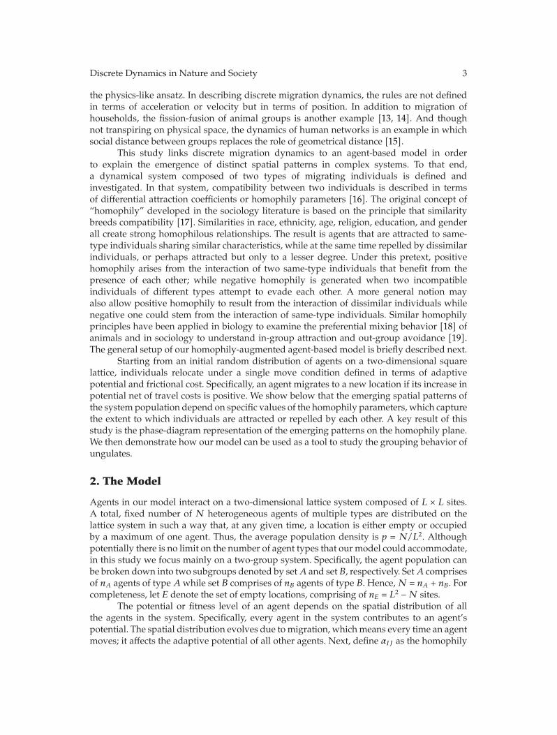
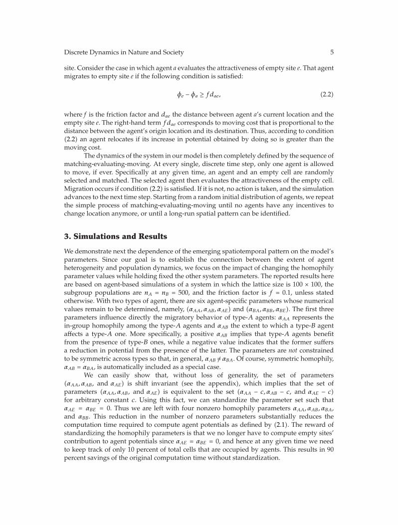
We show next the distinct spatiotemporal patterns that emerge from the systemcorresponding to different combinations of the two independent homophily parameters. Ingeneral, starting from a random initial distribution, the long-run behavior of the systemconverges toward two broad classes of temporal outcomes. Under some parameter setting,the system settles down to a stationary equilibrium pattern. Every agent in the systemis satisfied with its current location or, equivalently, there is no possible relocation thatwould make an agent profited from a move. This case therefore corresponds to the staticregime. Under some other parameter setting, however, the system never settles down.Instead, the system remains out of equilibrium even in the long run, with agents constantlymoving in a state of perpetual motion. This case corresponds to the dynamic nonequilibriumregime in which the prevailing spatial pattern is ever-changing. Figures 1 and 2 showexamples of spatial patterns that emerge under both stationary and dynamic regimes. A selectnumber of distinct patterns were already reported in a previous study [24]. Nevertheless, acomprehensive study establishing the link between patterns and the model parameters hasnot been done until now.

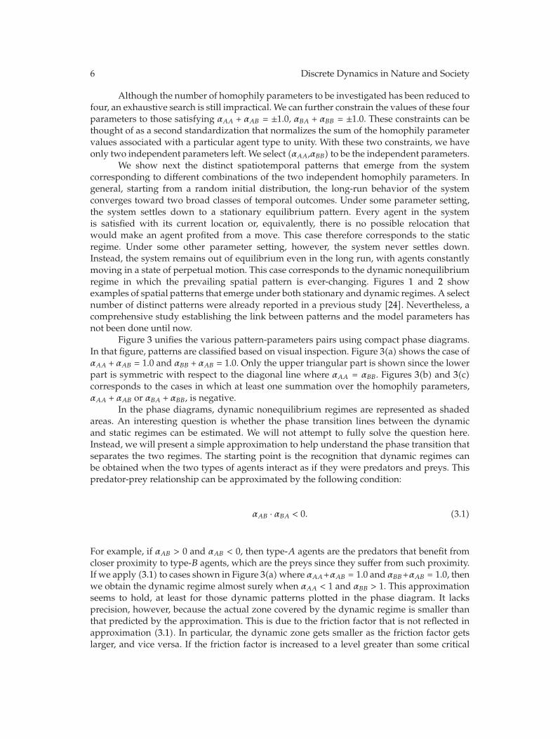
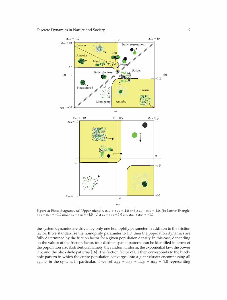
Figure 3 unifies the various pattern-parameters pairs using compact phase diagrams.In that figure, patterns are classified based on visual inspection. Figure 3(a) shows the case ofαAA + αAB = 1.0 and αBB + αAB = 1.0. Only the upper triangular part is shown since the lowerpart is symmetric with respect to the diagonal line where αAA = αBB. Figures 3(b) and 3(c)corresponds to the cases in which at least one summation over the homophily parameters,αAA + αAB or αBA + αBB, is negative.

In the phase diagrams, dynamic nonequilibrium regimes are represented as shadedareas. An interesting question is whether the phase transition lines between the dynamicand static regimes can be estimated. We will not attempt to fully solve the question here.Instead, we will present a simple approximation to help understand the phase transition thatseparates the two regimes. The starting point is the recognition that dynamic regimes canbe obtained when the two types of agents interact as if they were predators and preys. Thispredator-prey relationship can be approximated by the following condition:

αAB · αBA < 0. (3.1)

For example, if αAB > 0 and αAB < 0, then type-A agents are the predators that benefit fromcloser proximity to type-B agents, which are the preys since they suffer from such proximity.If we apply (3.1) to cases shown in Figure 3(a)where αAA+αAB = 1.0 and αBB+αAB = 1.0, thenwe obtain the dynamic regime almost surely when αAA < 1 and αBB > 1. This approximationseems to hold, at least for those dynamic patterns plotted in the phase diagram. It lacksprecision, however, because the actual zone covered by the dynamic regime is smaller thanthat predicted by the approximation. This is due to the friction factor that is not reflected inapproximation (3.1). In particular, the dynamic zone gets smaller as the friction factor getslarger, and vice versa. If the friction factor is increased to a level greater than some critical


(a) (b) (c) (d)

Figure 1: Stationary patterns: (a) separated, (b) ghetto, (c) mixed, and (d) stripes.

Figure 2: Dynamic patterns, from top to bottom: (a) cell, (b) worm, (c) herd, (d) amoeba, and (e) swarm.

value, the system is “frozen” in its initial state [16], which means the static regime triviallyrules the entire phase plane.

Table 1 lists the long-run patterns of the population spatial distribution found in thepresent study. It is important to keep in mind that the list is not meant to be exhaustive. Anumber of patterns were already identified and reported in a previous study [24], includingthe worm and the cell modes. However, the list also includes newly identified patterns suchas the herd, the amoeba, and the stripes modes. One contribution of this paper is the pinningdown of the patterns’ relative positions vis-a-vis others on the phase diagram. The cell patternin particular is fascinating since it can be thought of as representing self-replicating cellsin a live organism. In contrast to cellular automatons which may be considered the most


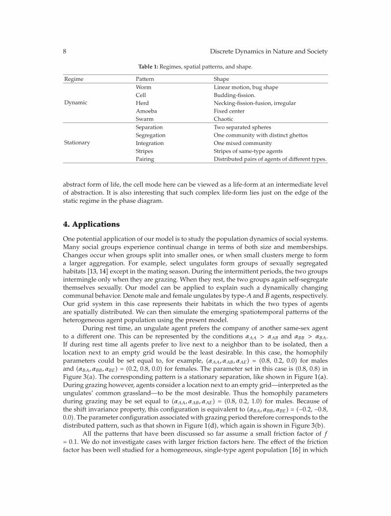
Table 1: Regimes, spatial patterns, and shape.

Regime Pattern Shape

Dynamic

Worm Linear motion, bug shapeCell Budding-fission.Herd Necking-fission-fusion, irregularAmoeba Fixed centerSwarm Chaotic

Stationary

Separation Two separated spheresSegregation One community with distinct ghettosIntegration One mixed communityStripes Stripes of same-type agentsPairing Distributed pairs of agents of different types.

abstract form of life, the cell mode here can be viewed as a life-form at an intermediate levelof abstraction. It is also interesting that such complex life-form lies just on the edge of thestatic regime in the phase diagram.

4. Applications

One potential application of our model is to study the population dynamics of social systems.Many social groups experience continual change in terms of both size and memberships.Changes occur when groups split into smaller ones, or when small clusters merge to forma larger aggregation. For example, select ungulates form groups of sexually segregatedhabitats [13, 14] except in the mating season. During the intermittent periods, the two groupsintermingle only when they are grazing. When they rest, the two groups again self-segregatethemselves sexually. Our model can be applied to explain such a dynamically changingcommunal behavior. Denote male and female ungulates by type-A and B agents, respectively.Our grid system in this case represents their habitats in which the two types of agentsare spatially distributed. We can then simulate the emerging spatiotemporal patterns of theheterogeneous agent population using the present model.

During rest time, an ungulate agent prefers the company of another same-sex agentto a different one. This can be represented by the conditions αAA > αAB and αBB > αBA.If during rest time all agents prefer to live next to a neighbor than to be isolated, then alocation next to an empty grid would be the least desirable. In this case, the homophilyparameters could be set equal to, for example, (αAA, αAB, αAE) = (0.8, 0.2, 0.0) for malesand (αBA, αBB, αBE) = (0.2, 0.8, 0.0) for females. The parameter set in this case is (0.8, 0.8) inFigure 3(a). The corresponding pattern is a stationary separation, like shown in Figure 1(a).During grazing however, agents consider a location next to an empty grid—interpreted as theungulates’ common grassland—to be the most desirable. Thus the homophily parametersduring grazing may be set equal to (αAA, αAB, αAE) = (0.8, 0.2, 1.0) for males. Because ofthe shift invariance property, this configuration is equivalent to (αBA, αBB, αBE) = (−0.2, −0.8,0.0). The parameter configuration associatedwith grazing period therefore corresponds to thedistributed pattern, such as that shown in Figure 1(d), which again is shown in Figure 3(b).

All the patterns that have been discussed so far assume a small friction factor of f= 0.1. We do not investigate cases with larger friction factors here. The effect of the frictionfactor has been well studied for a homogeneous, single-type agent population [16] in which


αAA = −10αBB = 10

αAA = 10

αBB = −10

Swarm

Swarm

Amoeba

Amoeba

Stripes

Static:mixed

Static: ghetto

HerdWorm

Static: segregation

Cell

0

0

0.5

2.6

(a) (b)−1.2

−0.9

Monogamy

0

(c)

−0.8

10

0

−1.5

−102

αAA = −10αBB = 10

αAA = 10

αBB = −10

0.5

Figure 3: Phase diagrams. (a) Upper triangle, αAA + αAB = 1.0 and αBA + αBB = 1.0. (b) Lower Triangle,αAA + αAB = −1.0 and αBA + αBB = −1.0. (c) αAA + αAB = 1.0 and αBA + αBB = −1.0.

the system dynamics are driven by only one homophily parameter in addition to the frictionfactor. If we standardize the homophily parameter to 1.0, then the population dynamics arefully determined by the friction factor for a given population density. In this case, dependingon the values of the friction factor, four distinct spatial patterns can be identified in terms ofthe population size distribution, namely, the random uniform, the exponential law, the powerlaw, and the black-hole patterns [16]. The friction factor of 0.1 then corresponds to the black-hole pattern in which the entire population converges into a giant cluster encompassing allagents in the system. In particular, if we set αAA = αBB = αAB = αBA = 1.0 representing


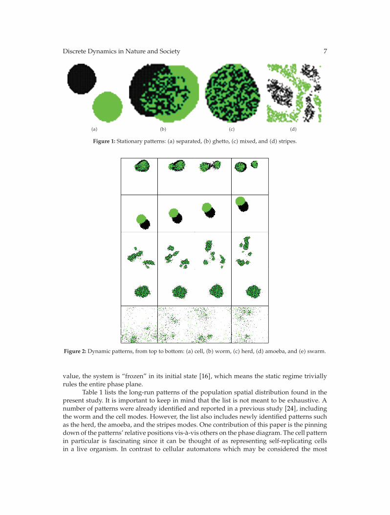
Figure 4: Distributed groups for large friction f = 0.45.

essentially a homogeneous population, then all agents regardless of type collapse to a singlegroup, that is, the black hole. The reason why in the present study we observe separatedgroups as shown in the phase diagram is due to negative, homophily parameters.

When the homophily parameters are all positive and the friction factor f = 0.1,we obtain at most two groups in the long run. But at higher friction factors we obtain adistributed system of groups—even with all-positive homophily parameters—where eachgroup can contain a mix of different types. An example is a multiracial city system. Cities insuch a system form spatially distributed groups, each composed of different types, that is,races. In a multiracial system the degree of segregation between the different races is often ofinterest. Another example is associated with mammalian groups. During the grazing period,ungulates self-organize themselves into smaller groups, each of which is sexually segregated.In order to quantify the overall degree of gender partitioning among ungulates, we computethe segregation coefficient (SC) as follows [14]

SC =

[1 − N

XY

K∑

i=1

xiyi

n i −1

]1/2

, (4.1)

where X and Y denote the total number of males and females in the system, respectively,and N = X + Y . There are K-groups in the system. In the ith group, the male and femalesubpopulations are denoted by x i and y i , respectively. Groups with only one member areexcluded from the calculation of the segregation coefficient. Our model can be easily appliedto see how segregation behavior responds to changes in the homophily parameters. Againconsider a population of ungulates where the group behavior of males is represented bythe parameters (αAA, αAB, αAE) = (0.8, 0.2, 0.0) while for females (αBA, αBB, αBE) = (0.2, 0.8,0.0). The friction factor is set at f = 0.45, much higher than before in order to focus on caseswhere ungulates migrate not solely because of homophily forces, in particular during grazingperiods when they strongly prefer to live next to an empty grassland.

With higher friction factor, the groups remain spatially distributed as shown inFigure 4. But the homophily forces remain sufficiently strong that each group exhibits unevendistribution of the two sexes. Note that we defined a “group” here as the cluster of locationsconnected by at least one non-empty site. From simulations of a 200 × 200 lattice system withX = 1600 and Y = 2400, we obtain the average SC equal to (mean, standard deviation) =


Figure 5: A Static pattern obtained from a three-color case.

(0.35, 0.045) and the average group size for ni ≥ 2 is 3.2. The segregation coefficientclearly suggests the tendency for males and females to live in gender-partitioned groups.Changing the male homophily parameter values to (0.7, 0.3, and 0.0) reduces the segregationcoefficient to (0.16, 0.051). Thus, we could calibrate the parameters in order to fit the availableexperimental data and then perform simulations to test whether sexual homophily causesgender segregation, but not the other way around. Finally, we can also apply the model toa heterogeneous population with more than two types of agents. In Figure 5, we presentan interesting spatial pattern generated from a system with three agent types. With greaternumber of parameters, more complex patterns could be generated.

5. Concluding Remarks

We have developed an agent-based model to investigate how diverse spatial patterns can begenerated from a minimal set of interaction rules. Numerical simulations of the model allowus to identify distinct stationary and dynamic patterns of the population spatial distribution,and we present phase diagrams on the planes of homophily parameters. The complexspatial patterns are generated primarily by agents’ simple adaptive behavior, and not by theinternal complexity of the agents themselves. The phase transition between the dynamic andstationary regimes is also identified and explained. Our model can be applied to study thegroup forming behavior of social communities. As an example, we apply themodel to explainthe sexual segregation of ungulates in terms of the homophily parameters and the frictionfactor. Future extensions of this study could include the development of the generalizedSchelling model of segregation in a heterogeneous population with n types of agents. Also itwill be an interesting topic of research to classify social systems in terms of the various spatialpatterns of the population associated with the dynamic regime presented in this study.

Appendix

The Shift Invariance of Homophily Parameters

This appendix shows that the set of parameters (αAA, αAB, and αAE) is indeed shift invariant,which implies that the set (αAA, αAB, αAE) is equivalent to the set (αAA − c, αAB − c, αAE − c) foran arbitrary constant c.


By definition, the potential of an agent a of type A is given by the following equation:

φa =j /= i∑

j=1,L2

αIJ

dνij

=j /= i∑

j={A}

αAJ

dνij

+∑

j={B}

αAJ

dνij

+∑

j={E}

αAJ

dνij

. (A.1)

In (A.1), the sets {A}, {B}, and {E} correspond to agents of type A and B, as wellas empty cells, respectively. Now, subtracting a constant c from every homophily parameteryields

φa(αAA − c, αAB − c, αAE − c) =j /=a∑

j=1,L2

(αIJ − c

)

dνij

=j /=a∑

j∈{A}

(αAJ − c

)

dνij

+∑

j∈{B}

(αAJ − c

)

dνij

+∑

j∈{E}

(αAJ − c

)

dνij

=j /=a∑

j={A}

αAJ

dνij

+∑

j={B}

αAJ

dνij

+∑

j={E}

αAJ

dνij

−j /=a∑

j∈{A+B+E}

c

dνij

= φa(αAA, αAB, αAE) − cj /=a∑

j∈{A+B+E}

1dνij

.

(A.2)

Similarly, the potential of an agent b of type B is obtained as follows:

φb(αAA − c, αAB − c, αAE − c) = φb(αAA, αAB, αAE) − cj /= b∑

j∈{A+B+E}

1dνij

. (A.3)

Since we are dealing with systems exhibiting periodic boundaries, it follows that

j /=a∑

j∈{A+B+E}

1dνij

=j /= b∑

j∈{A+B+E}

1dνij

= K, (A.4)

where K is a constant, which does not depend on the specific agent under consideration.Thus, it follows that

φi(αIA − c, αIB − c, αIE − c) = φi(αIA, αIB, αIE) −K′, ∀i ∈ {A,B}, (A.5)

where K′ = cK is just another constant. This proves that the parameter sets (αAA − c, αAB −c, αAE − c) and (αAA, αAB, αAE) are equivalent. Therefore, (αAA − c, αAB − c, αAE − c) and(αAA, αAB, αAE) are shift invariant. This completes the proof.

Acknowledgment

This research was supported by the Yeungnam University research grants in 2009.


References

[1] J. A. Glazier and F. Graner, “Simulation of the differential adhesion driven rearrangement of biologicalcells,” Physical Review E, vol. 47, no. 3, pp. 2128–2154, 1993.

[2] P. Hogeweg, “Evolving mechanisms of morphogenesis: on the interplay between differentialadhesion and cell differentiation,” Journal of Theoretical Biology, vol. 203, no. 4, pp. 317–333, 2000.

[3] R. Vabø and L. Nøttestad, “An individual based model of fish school reactions: predictingantipredator behaviour as observed in nature,” Fisheries Oceanography, vol. 6, no. 3, pp. 155–171, 1997.

[4] S. V. Viscido, J. K. Parrish, and D. Grunbaum, “The effect of population size and number of influentialneighbors on the emergent properties of fish schools,” Ecological Modelling, vol. 183, no. 2-3, pp. 347–363, 2005.

[5] F. Schweitzer, Brownian Agents and Active Particles, Springer, Berlin, Germany, 2003.[6] D. Helbing and P. Molnar, “Social force model for pedestrian dynamics,” Physical Review E, vol. 51,

no. 5, pp. 4282–4286, 1995.[7] C. Langton, Artificial Life: An Overview, MIT Press, Cambridge, Mass, USA, 1995.[8] C. W. Reynolds, “Flocks, herds and schools, a distributed behavioral model,” Computer Graphics, vol.

21, no. 4, pp. 25–34, 1987.[9] S. Levy, Artificial life: A Report from the Frontier Where Computers Meet Biology, Vintage Books, Random

House, New York, NY, USA, 1992.[10] T. Schelling, “Dynamic models of segregation,” Journal of Mathematical Sociology, vol. 1, pp. 143–186,

1971.[11] J. K. Shin andM. Fossett, “Residential segregation by hill-climbing agents on the potential landscape,”

Advances in Complex Systems, vol. 11, no. 6, pp. 875–899, 2008.[12] S. Kaufman, The Origins of Order: Self-Organization and Selection in Evolution, Oxford University Press,

New York, NY, USA, 1993.[13] L. Conradt and T. J. Roper, “Activity synchrony and social cohesion: a fission-fusion model,”

Proceedings of the Royal Society B, vol. 267, no. 1458, pp. 2213–2218, 2000.[14] K. E. Ruckstuhl and P. Neuhaus, “Sexual segregation in ungulates: a new approach,” Behaviour, vol.

137, no. 3, pp. 361–377, 2000.[15] J. A. Holyst, K. Kacperski, and F. Schweitzer, “Phase transitions in social impact models of opinion

formation,” Annual Reviews of Computational Physics, vol. 9, pp. 253–273, 2001.[16] J. K. Shin, G. S. Shin, and Y. S. Mansury, “Clustering in a spatial system of self-aggregating agents,”

Fractals, vol. 17, no. 1, pp. 99–107, 2009.[17] M. McPherson, L. Smith-Lovin, and J. M. Cook, “Birds of a feather: homophily in social networks,”

Annual Review of Sociology, vol. 27, pp. 415–444, 2001.[18] D. Lusseau, B. Wilson, P. S. Hammond et al., “Quantifying the influence of sociality on population

structure in bottlenose dolphins,” Journal of Animal Ecology, vol. 75, no. 1, pp. 14–24, 2006.[19] S.-S. Hwang and S. H. Murdock, “Racial attraction or racial avoidance in American suburbs?” Social

Forces, vol. 77, no. 2, pp. 541–566, 1998.[20] K. Kaneko, Life: An Introduction to Complex Systems Biology, Springer, Berlin, Germany, 2006.[21] H.-S. Niwa, “Newtonian dynamical approach to fish schooling,” Journal of Theoretical Biology, vol. 181,

no. 1, pp. 47–63, 1996.[22] I. D. Couzin and J. Krause, “Self-organization and collective behavior in vertebrates,” Advances in the

Study of Behavior, vol. 32, pp. 1–75, 2003.[23] Y. Mansury, M. Kimura, J. Lobo, and T. S. Deisboeck, “Emerging patterns in tumor systems:

simulating the dynamics of multicellular clusters with an agent-based spatial agglomeration model,”Journal of Theoretical Biology, vol. 219, no. 3, pp. 343–370, 2002.

[24] J. K. Shin, “Emergence of static and dynamic patterns on two-color slope system,” Fractals, vol. 15,no. 3, pp. 237–247, 2007.

Emerging Spatiotemporal Patterns from Discrete Migration...

Documents

Transcript of Emerging Spatiotemporal Patterns from Discrete Migration...