Emergency Nutrition Assessment for Standardized Monitoring and Assessment of Relief and Transitions

(ENA for SMART)

Software User Manual

ENA 2011 (Version 2011, July 31st, 2012)

Final Version August 2012

1

TABLE OF CONTENTS TABLE OF CONTENTS ............................................................................................................. 1 ACKNOWLEDGEMENTS .......................................................................................................... 3 INTRODUCTION ..................................................................................................................... 4 1. GETTING STARTED .......................................................................................................... 5

1.1 Installation of the Software ............................................................................................. 5 1.2 Opening the Software ...................................................................................................... 6 1.3 Getting to Know the Software ......................................................................................... 6

1.3.1 Files .............................................................................................................................. 7 1.3.2 Extras ............................................................................................................................ 8

2. PLANNING ................................................................................................................... 11 2.1 Name of Survey .............................................................................................................. 11 2.2 Sampling ......................................................................................................................... 12 2.3 Sample Size Calculation for a Cross Sectional Anthropometric Survey ......................... 14 2.4 Sample Size Calculation for a Death Rate Survey .......................................................... 18 2.5 Table for Cluster Sampling ............................................................................................. 19 2.6 Random Number Table .................................................................................................. 20

3. TRAINING..................................................................................................................... 23 3.1 Type of data: .................................................................................................................. 23 3.2 Data entry ...................................................................................................................... 24 3.3 Data analysis and reporting ........................................................................................... 24

4. DATA ENTRY ANTHROPOMETRY ................................................................................... 27 4.1 Shortcuts ........................................................................................................................ 28 4.2 Individual results ............................................................................................................ 28 4.3 Column variable ............................................................................................................. 29 4.4 Row/Data ....................................................................................................................... 29 4.5 Go To (Selecting records) ............................................................................................... 29 4.6 Report plausibility check report ..................................................................................... 29 4.7 NCHS reference and WHO standards ............................................................................ 30 4.8 Disclaimer ....................................................................................................................... 30 4.9 Data entry screen ........................................................................................................... 30 4.10 Variable view .................................................................................................................. 31

5. RESULTS ANTHROPOMETRY ......................................................................................... 35 5.1 Statistical calculator ....................................................................................................... 42

5.1.1 Analysing a single variable ......................................................................................... 43 5.1.2 Analysing variables using crossable ........................................................................... 44 5.1.3 Calculating prevalence estimates with design effect and adjusted confidence intervals .................................................................................................................................. 45

6. DEATH RATES ............................................................................................................... 47 6.1 Data Entry Individual Level ............................................................................................ 47

6.1.1 Shortcuts .................................................................................................................... 47 6.1.2 Recall days .................................................................................................................. 48

2

6.1.3 Cause and location of death ...................................................................................... 49 6.1.4 Data entry ..................................................................................................................... 49 6.1.5 Data of all household .................................................................................................... 50

6.2 Results individual level ................................................................................................... 51 6.2.1 Age groups for evaluation (years) .............................................................................. 52 6.2.2 Summary table for age groups................................................................................... 52 6.2.3 Summary table for clusters ........................................................................................ 52 6.2.4 Death rates and design effects .................................................................................. 52 6.2.5 Population pyramid and transfer table to Excel ........................................................ 53

6.3 Data entry household level ............................................................................................ 53 6.3.1 Shortcuts .................................................................................................................... 53 6.3.2 Recall days from planning sheet ................................................................................ 53 6.3.3 Spread sheet for data entry ....................................................................................... 54

6.4 Results household level ................................................................................................. 55 7. OPTIONS ...................................................................................................................... 57

7.1 Automatic fill out ........................................................................................................... 58 7.2 Entering of age ............................................................................................................... 58 7.3 7.3 Entering of date ....................................................................................................... 58 7.4 Showing columns for measure, cloths, and weighing variables .................................... 58 7.5 Program for output ........................................................................................................ 61 7.6 Age groups ..................................................................................................................... 61 7.7 Exclusion of z-scores ...................................................................................................... 61 7.8 Anthropometry analysing criteria .................................................................................. 62 7.9 MUAC cut-off ................................................................................................................. 62 7.10 Reset and save ............................................................................................................... 62

Annex 1: Death Rate Survey Form ........................................................................................ 63 Annex 2: Converting sample size from children to households ............................................. 64 Annex 3: Answers to exercises ............................................................................................. 66

3

ACKNOWLEDGEMENTS This manual was written by Douglas Jayasekaran with guidance and support from Aurore Virayie. The manual has been reviewed by Melody Tondeur, Hermann Ouedraogo, Yara Sfeir, and Victoria Sauveplane. ACF Canada would like to thank US AID for the financial support for developing this manual.

4

INTRODUCTION

Standardized Monitoring and Assessment of Relief and Transitions (SMART) is a survey methodology that was developed to improve the quality of anthropometric and mortality survey data collected in humanitarian and development contexts (however, SMART has been increasingly used in developmental settings). The aim of SMART is to assist decision-makers to carry out, analyse, interpret, and report on survey findings in a standardized manner while maintaining the reliability of the data. In order to assist field workers to carry out surveys using the SMART methodology, several tools have been developed. These tools include, a SMART survey manual (April 2006), an accompanying computer software programme namely Emergency Nutrition Assessment (ENA), a Standardised Training Package (STP1), and a sampling guide. ENA is a computer software programme that was developed to facilitate the planning, data collection, analysis, and reporting of anthropometric, mortality, and food security survey data in a standardised and simplified manner. ENA software, which originally came out as NutriSurvey for SMART Emergency Nutrition Assessment has gone through several updates based on user feedback and best practises in the field and the current edition of the software is ENA 2011 (Version 2011, July 31st, 2012). This ENA software user manual has been developed to guide the ENA 2011 (Version 2011, July 31st, 2012) users. The main purpose of the manual is to provide users with an understanding of various functionalities of the ENA 2011 software so that they will be able to use the software to plan and implement surveys and analyse survey data. This manual does not describe the theories behind the functionalities used in the software or the SMART methodology itself. The manual should be used along with the SMART manual (April 2006), the STP, and the sampling guide to get a better understanding of the various concepts used in the software. Although a food security module is included in the ENA 2011 software, this manual does not include information about how to use the food security module in the software as guidance on how to carry out food security surveys are still being finalised. It is hoped that this manual will be revised as the ENA software is updated. Additional information about the ENA software can be found on: www.nutrisurvey.de/ena2011. For further information on the SMART methodology, please visit: www.smartmethodology.org.

1Standardised Training Package (STP) is a set of Microsoft PowerPoint presentations that has been developed by ACF Canada to help organise and deliver training on the SMART methodology. The STP has been tested and peer-reviewed and can be found on: http://www.smartmethodology.org/index.php/article/index/capacity_building_ toolbox/stp Reference is made to various STP modules throughout this manual.

5

1. GETTING STARTED

1.1 Installation of the Software The ENA 2011 (Version 2011, July 31st, 2012) software can be downloaded for free from the following web page: http://www.smartmethodology.org/ (by clicking on the ENA Software which can be found on the right hand side of the Capacity building toolbox section) or from this web link: http://www.nutrisurvey.de/ena2011/2. Alternatively, a ZIP file with the ena.exe file can be downloaded from the following web link: www.nutrisurvey.net/ena2011/ena2011.zip and ENA software can be installed by running the ena.exe in the ZIP file. The default installation directory for the ena.exe file is set to be the c: directory (i.e. c:/ena2011). This should work in most cases. Once the installation is complete, an icon (see below) will be displayed on the computer desktop.

ENA 2011 software icon as it appears on the computer desktop

During the installation of the software, a folder named ena2011 will be automatically created in the c:/ drive and all the ENA 2011 software programme related files will be stored in this folder. The ena2011 folder will also act as the default folder for saving the survey data files (i.e. when files are saved for the first time, ena2011 folder will be selected for saving the files). If an ENA 2011 file needs to be saved in another folder, it should be manually selected while saving the file. The file extension used in ENA 2011 data files is .as. There should not be any space in the folder name ena2011 (i.e. no space between the word ‘ena’ and the number ‘2011’) as this space may cause problems either with installations or proper functioning of the software. If there is a space, make sure to manually remove it during the installation. In some cases, if the Microsoft Office 2010 version is installed in the computer after ena2011 was installed, this may also affect the smooth functionality of the ena2011 software. In these situations, uninstall the ena2011 software and reinstall it in the computer’s Programme files after Microsoft Office 2010 installation is complete. 2 This web link can also be used to download older versions of the software such as ENA 2007 and ENA2008.

6

1.2 Opening the Software The software can be accessed by double clicking on the ‘ENA for SMART’ icon on the desktop or by clicking on the <Start> menu and selecting the ENA for SMART programme under <All Programmes>. When opening the software, the software will first open with the box displaying the names of the individuals who designed the software along with what version of the software – e.g. July 31, 2012. It is recommended that the latest version is always used as it will always

have the most advanced features; the latest version currently is ENA 2011 (July 31, 2012). The box will also show an email contact where feedback and queries can be sent to and the link to the web page where the software is housed. Note that feedback can also be sent to the SMART forum on: www.smartmethodology.org web page. When ready to go into the software, click on <OK> to proceed. 1.3 Getting to Know the Software Figure 1.1: Screenshot of files menu as it is opened on a data entry anthropometry screen

When the software is opened, it automatically opens up with the Date Entry Anthropometry screen (see section 4 below). However, the software also has other screens such as planning, Training, Results Anthropometry, Death Rates, Food Security, and Options, which are arranged

7

in an order following the steps of a typical SMART survey. Additionally, there is a menu bar for Files and Extras with further commands. The Files and Extras menu are described here and each screen (except food security screen) is illustrated below in the subsequent sections. 1.3.1 Files The Files menu consists of 6 commands grouped into 3 sections. Some of these commands are also available in the shortcuts on data entry anthropometry screen (e.g. New, Open, and Save) and death rate survey screen (e.g. Save) – see respective sections below for details. The Files menu also has the names and paths of up to 4 files that have recently been used (note: when the software is opened and used for the first time, this information will not be available). The functionality of each command in the Files menu is described below. Table 1.1: Functions of commands in the Files menu

Command Function Remarks

New Opens a new file in .as format

Regardless of the screen on display when this command is clicked, the software will always open up a new Data Entry Anthropometry screen. If there is unsaved data when this command is selected, the software will ask whether the data needs to be saved. If the (unsaved) data doesn’t need to be saved, click on <No> and a new file will open up. If the data needs to be saved, click <Yes>. If a file has already been created, the data will be saved in the file and a new file will be opened. If no file has been previously created, a new window will appear showing the recommended file name format. If the data needs to be saved, click <OK> and save the data in the recommended file name format (see below). Once the file is saved, a new file will be opened.

Open Opens an existing .as file

A new window will be opened displaying the contents of the ena2011 folder. When a file is open, the path to the file is displayed on the top of the screen. If there is unsaved data when this command is selected, the software will ask whether the data needs to be saved. Follow the instructions above under the command <New> to save the data.

Save Saves the actual file in .as format

If a file has already been created, the data will be saved in the file. If the data is saved for the first time, a new window with the recommended file name format will appear. Click <OK> to proceed. Save the file based on the recommended file name format (see below).

Save as Saves file .as with a chosen name

A new window with the recommended file name format will appear. Click <OK> to proceed. Save the file based on the recommended file name format (see below).

8

Import EPI-Info 5/6 or DBase files

Imports files .rec EPI-Info (.rec) 5/6 or DBase (.dbf) file

This function was included to facilitate the import and analysis of data in .rec and .dbf file formats. As Windows versions of EPI-info are increasingly used, this functionality maybe removed in the next version of ENA. To import a .rec or .dbf file, click on the command and select the file to be imported from the window that is displayed. Click on <OK>.

Exit Closes the software If there is unsaved data, a new window asking whether to save the data will appear when <Exit> is clicked. Click <Yes> if the data needs to be saved. If not, click <Cancel>. If <Yes> is selected, a new window will appear showing the recommended file name format. Select <Yes> and save the file in the recommended file name format (see below). If <Cancel> is selected at this stage, the software will close and all unsaved data will be lost!

1.3.2 Extras Figure 1.2: Screenshot of Extras menu as it is opened on a data entry anthropometry screen

The Extras menu has 11 commands some of which are also available in the shortcuts in the training data entry anthropometry and death rate screens. Each of the command is briefly described below. For additional information, refer to the respective sections indicated.

9

Table 1.2: Functions of commands in the Extras menu

Command Function

Form for anthropometric

survey

Opens an anthropometric survey questionnaire in Microsoft Word format; the form is identical to the Data Entry Anthropometry screen (see below). This is a very basic form designed to collect anthropometric data quickly in an emergency situation. The form structured in a way that data from children in an entire cluster can be collected in one form. If additional data are to be collected, this form should be adapted. It may also be useful to design the form in a format that can capture information from each household, including anthropometry, separately (i.e. one form per household). See STP module 1 or contact the SMART forum for additional details on questionnaire design.

Form for death rate

survey

Provides options for 2 types of death rate survey forms: 1) SMART standard form and 2) Simple form (one sheet/cluster). Both of these forms have shortcomings and their use is discouraged. For the form that is currently recommended for use in a death rate survey, see annex 1.

Paste Data from Clipboard Pastes data that was copied last into the spread sheet on Data Entry Anthropometry screen. This function is similar to paste function in Microsoft Office packages and can also be executed by pressing <Ctrl> + <V> keys together on the keyboard (data will be pasted on the highlighted cell in the data entry anthropometry screen) however, pasting by right-clicking the mouse and selecting paste option does not work in ENA. To paste data onto a specific screen, the shortcut button for paste on the specific screen needs to be selected (see below). For example, to paste data onto training screen, the shortcut button for paste on the training screen needs to be clicked.

Transfer survey data to

Excel

The data in the Data Entry Anthropometry will be exported to Excel along with column headings (see section on Data Entry Anthropometry). To transfer data on a specific screen, the shortcut button for transfer on the specific screen needs to be selected (see below). For example, to transfer data on death rate survey screen, the shortcut button for paste on the death rate survey screen needs to be clicked. Note that although the data is transferred to a Excel template, the file format used in ENA 2011 is a text (.txt). It is recommended that the transferred file is saved in Microsoft Workbook (.xls) file format. To do this, follow the standards procedure for saving a document. In the small window that appears, type the file name and from the dropdown button for ‘save as type’ select <Excel Workbook>.

Plausibility check Opens plausibility report in Microsoft Word format (see section on

10

Data Entry Anthropometry).

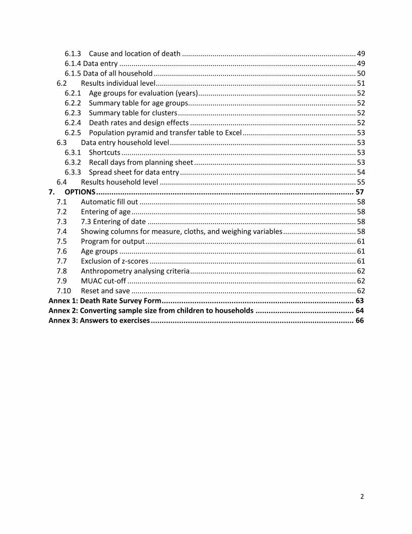
Check of double entry Compares two data files and check if they are similar. It is used in data entry to make sure the survey data was entered correctly (see section on Data Entry Anthropometry).

Report in Word Generates a sample report template with standard tables that are automatically filled with anthropometric and death rate survey data.

Statistical calculator Allows further analysis and cross-tabulation of variables (see section on Results Anthropometry)

Weighted analysis of

survey

Facilitates analysis of survey data where weighing needs to be taken into account because of unequal probability of selection for different elements in the sample (see section on Data Entry Anthropometry). This is typically done when combining 2 or more surveys.

Merge surveys Enables 2 different datasets to be merged into one dataset (see section on Data Entry Anthropometry)

Change of language Changes the software between English and French. To change language, select the <Change of language> command in the <Extras> menu. A box will appear with 2 language options (english.Ing and French.Ing). Select the language and press <OK>. Once the language is changed the software must be restarted to effect the changes. ENA in other languages may also be made available to users upon request – please post the request on the SMART forum on www.smartmethodology.org.

Notes:________________________________________________________________________

______________________________________________________________________________

______________________________________________________________________________

______________________________________________________________________________

______________________________________________________________________________

______________________________________________________________________________

______________________________________________________________________________

______________________________________________________________________________

______________________________________________________________________________

______________________________________________________________________________

______________________________________________________________________________

______________________________________________________________________________

______________________________________________________________________________

______________________________________________________________________________

11

2. PLANNING The Planning section of the software is used to calculate sample sizes for anthropometric and death rate surveys and, in a cluster survey, is used to assign clusters. The planning screen can also be used to generate random number tables. Figure 2.1: Screenshot of ENA 2011 planning screen

For illustration purposes, the planning screen has been divided into following 6 sections: 1) Name of survey, 2) Sampling, 3) Sample size calculation for a cross sectional anthropometric survey, 4) Sample size calculation for a death rate survey, 5) Table for cluster sampling, and 6) Random number table. Each section is described in detail below. 2.1 Name of Survey

This section allows one to give a name for the survey. It is important

that each survey is identified by a unique name and all files and

directories associated with the survey are named consistently so

that it can be easily recognized by any of the team members.

1 2

3

4

5

6

12

It is recommended that the file name starts with the 3 letter country code (e.g., SUD for Sudan,

ZAM for Zambia, ANG for Angola, etc.), followed by the date of the survey in YYMM format. It

may also be useful to include the following information: the region, type of population

(refugee, IDP, resident), and the agency involved. It is also useful to include the type of file (REP

for report, DAT for the data file, etc.) when saving files.

Example 2.1: A file named <LIB_0408_IDP_Buchanan_AAH> would be the name of a survey conducted by Action Against Hunger among the IDPs in Buchanan, Liberia in September 2004. Similarly, a file named <LIB_0408_IDP_Buchanan_AAH_dat.xls> would be the data file of the above mentioned survey conducted by Action Against Hunger among the IDPs in Buchanan, Liberia in September 2004.

Exercise 2.1: A SMART survey was conducted by ACF in Dadu district of Pakistan in Oct. 2010. As the Survey Manager how would you: a) Name the survey?____________________________________________________________

b) Name the ENA (i.e. .as) file?____________________________________________________

c) Name the survey report?______________________________________________________

Compare your answers with the answers in Annex 3.

Note that the name that is given on the Planning screen (i.e. section no 1 above) is the survey

name that will be unique to each survey. The information entered in the ENA software needs to

be saved separately as an .as file3. It is recommended that planning and training data related to

one survey is saved in the same file along with anthropometric (and death rate survey data, if

applicable).

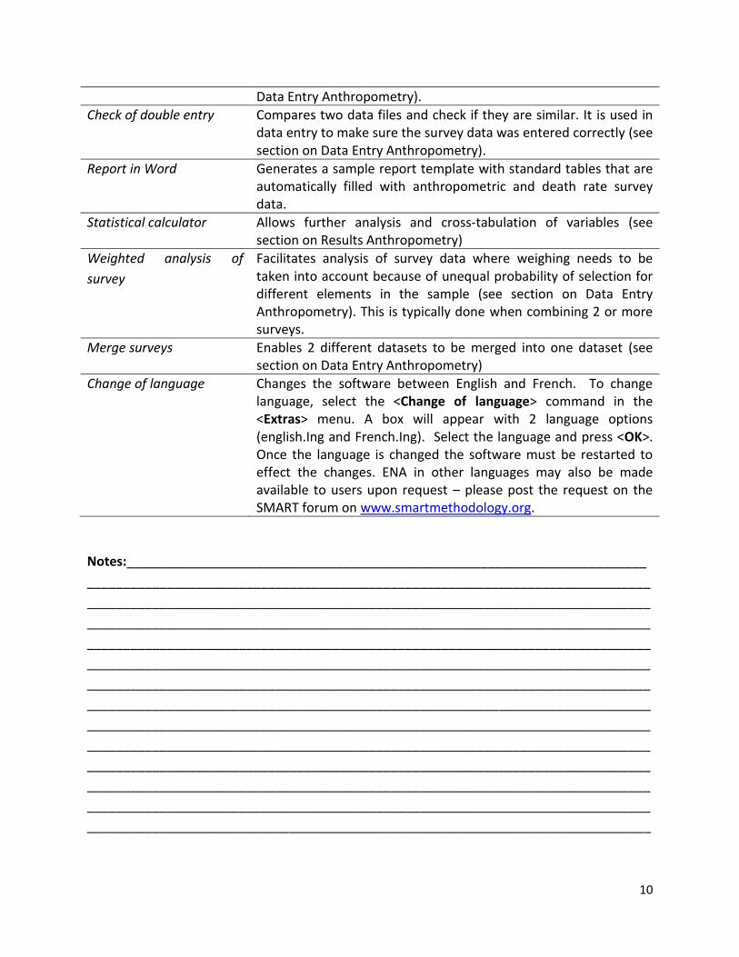
2.2 Sampling This section in the Planning screen helps specify what type of

sampling is to be used in the survey and whether a correction

factor (required for small population size) needs to be applied.

The default setting is always cluster but this needs to be

changed to random if the survey is going to use simple

random sampling method as this has implications in the sample size calculations (see below).

3To save a data file, click on the <Save as> command in the <Files> menu and save the file using the recommended file name format

13

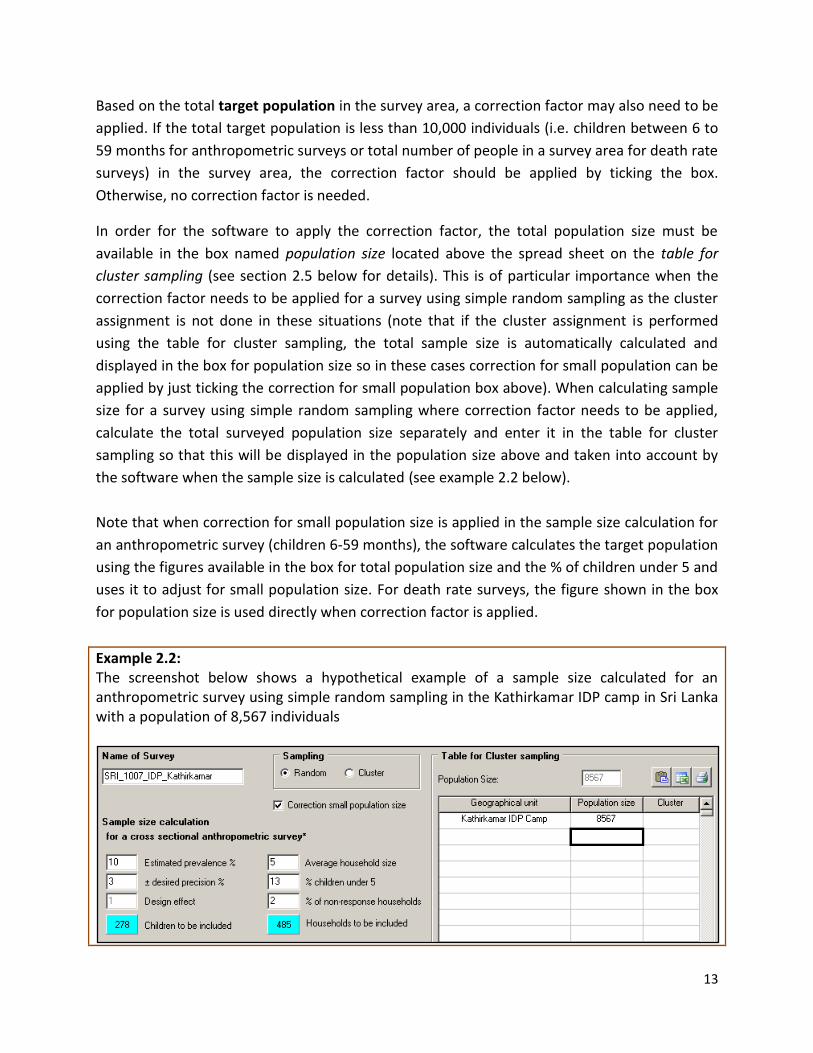
Based on the total target population in the survey area, a correction factor may also need to be

applied. If the total target population is less than 10,000 individuals (i.e. children between 6 to

59 months for anthropometric surveys or total number of people in a survey area for death rate

surveys) in the survey area, the correction factor should be applied by ticking the box.

Otherwise, no correction factor is needed.

In order for the software to apply the correction factor, the total population size must be

available in the box named population size located above the spread sheet on the table for

cluster sampling (see section 2.5 below for details). This is of particular importance when the

correction factor needs to be applied for a survey using simple random sampling as the cluster

assignment is not done in these situations (note that if the cluster assignment is performed

using the table for cluster sampling, the total sample size is automatically calculated and

displayed in the box for population size so in these cases correction for small population can be

applied by just ticking the correction for small population box above). When calculating sample

size for a survey using simple random sampling where correction factor needs to be applied,

calculate the total surveyed population size separately and enter it in the table for cluster

sampling so that this will be displayed in the population size above and taken into account by

the software when the sample size is calculated (see example 2.2 below).

Note that when correction for small population size is applied in the sample size calculation for

an anthropometric survey (children 6-59 months), the software calculates the target population

using the figures available in the box for total population size and the % of children under 5 and

uses it to adjust for small population size. For death rate surveys, the figure shown in the box

for population size is used directly when correction factor is applied.

Example 2.2: The screenshot below shows a hypothetical example of a sample size calculated for an anthropometric survey using simple random sampling in the Kathirkamar IDP camp in Sri Lanka with a population of 8,567 individuals

14

2.3 Sample Size Calculation for a Cross Sectional Anthropometric Survey The sample size calculation in

ENA can be described in 2 parts:

1) the left hand side that is used to calculate the number of subjects (i.e. sample size)

2) the right hand side that is used to calculate the number of households to visit in view to meet the calculated number of subjects, taking into account the average household size, percentage of survey subjects in a household, and the expected non-response rate.

In a SMART anthropometric survey, the survey subjects are children between 6-59 months and

the survey units are households. Thus, the sample size is first calculated in number of children,

which is then converted into number of households.

Note that the sample size calculation (left hand side) in ENA is similar to any categorical variable

(and thus can be used to calculate sample size for any variable with a proportion). For example

the left hand side of the sample size calculator can be used to calculate sample sizes for IYCF

indicators. However, the calculated number of households is only applicable to children 6-59

months. If the sample size calculation is performed for children aged 0-59 months, the

calculated number of households has to be multiplied by 0.9. The same applies when the right

hand side of the calculator is used to convert the sample size into number of households for

other age groups or target population (e.g. women of childbearing age).

In order to calculate the sample size, information about 5-6 factors (depending on the type of

sampling method used) are needed (see STP module 3 for details). Note that the values

included in the planning page are for illustration purposes only. These values will vary from

survey to survey and must be adjusted depending on the survey objectives.

Once the survey is named, type of sampling is specified, and decision about correction factor is

made (and applied as relevant), proceed according to the following steps to calculate the

sample size.

15

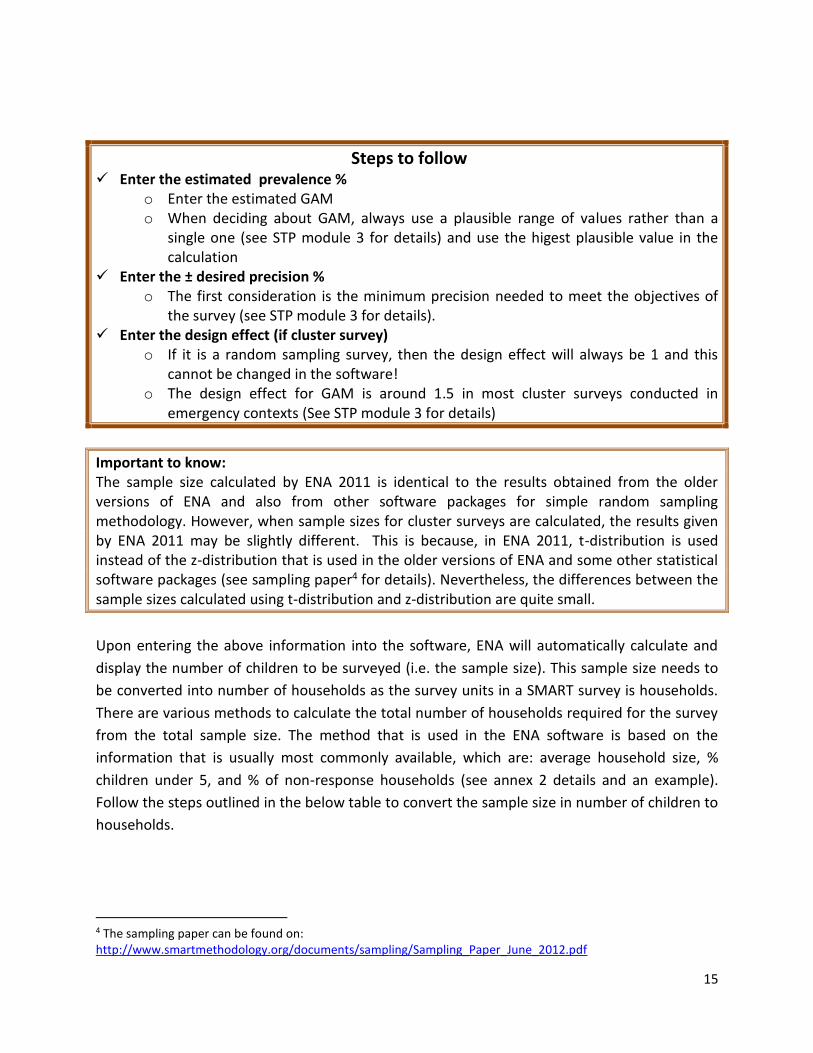
Steps to follow

Enter the estimated prevalence % o Enter the estimated GAM o When deciding about GAM, always use a plausible range of values rather than a

single one (see STP module 3 for details) and use the higest plausible value in the calculation

Enter the ± desired precision % o The first consideration is the minimum precision needed to meet the objectives of

the survey (see STP module 3 for details). Enter the design effect (if cluster survey)

o If it is a random sampling survey, then the design effect will always be 1 and this cannot be changed in the software!

o The design effect for GAM is around 1.5 in most cluster surveys conducted in emergency contexts (See STP module 3 for details)

Important to know: The sample size calculated by ENA 2011 is identical to the results obtained from the older versions of ENA and also from other software packages for simple random sampling methodology. However, when sample sizes for cluster surveys are calculated, the results given by ENA 2011 may be slightly different. This is because, in ENA 2011, t-distribution is used instead of the z-distribution that is used in the older versions of ENA and some other statistical software packages (see sampling paper4 for details). Nevertheless, the differences between the sample sizes calculated using t-distribution and z-distribution are quite small.

Upon entering the above information into the software, ENA will automatically calculate and

display the number of children to be surveyed (i.e. the sample size). This sample size needs to

be converted into number of households as the survey units in a SMART survey is households.

There are various methods to calculate the total number of households required for the survey

from the total sample size. The method that is used in the ENA software is based on the

information that is usually most commonly available, which are: average household size, %

children under 5, and % of non-response households (see annex 2 details and an example).

Follow the steps outlined in the below table to convert the sample size in number of children to

households.

4 The sampling paper can be found on: http://www.smartmethodology.org/documents/sampling/Sampling_Paper_June_2012.pdf

16

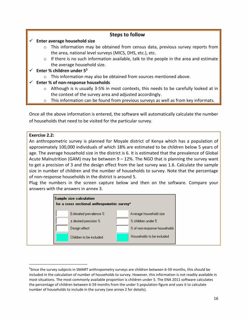
Steps to follow Enter average household size

o This information may be obtained from census data, previous survey reports from the area, national level surveys (MICS, DHS, etc.), etc.

o If there is no such information available, talk to the people in the area and estimate the average household size.

Enter % children under 55 o This information may also be obtained from sources mentioned above.

Enter % of non-response households o Although is is usually 3-5% in most contexts, this needs to be carefully looked at in

the context of the survey area and adjusted accordingly. o This information can be found from previous surveys as well as from key informats.

Once all the above information is entered, the software will automatically calculate the number

of households that need to be visited for the particular survey.

Exercise 2.2: An anthropometric survey is planned for Moyale district of Kenya which has a population of approximately 100,000 individuals of which 18% are estimated to be children below 5 years of age. The average household size in the district is 6. It is estimated that the prevalence of Global Acute Malnutrition (GAM) may be between 9 – 12%. The NGO that is planning the survey want to get a precision of 3 and the design effect from the last survey was 1.6. Calculate the sample size in number of children and the number of households to survey. Note that the percentage of non-response households in the district is around 5. Plug the numbers in the screen capture below and then on the software. Compare your answers with the answers in annex 3.

5Since the survey subjects in SMART anthropometry surveys are children between 6-59 months, this should be

included in the calculation of number of households to survey. However, this information is not readily available in most situations. The most commonly available proportion is children under 5. The ENA 2011 software calculates the percentage of children between 6-59 months from the under 5 population figure and uses it to calculate number of households to include in the survey (see annex 2 for details).

17

Notes:________________________________________________________________________

______________________________________________________________________________

______________________________________________________________________________

______________________________________________________________________________

______________________________________________________________________________

______________________________________________________________________________

______________________________________________________________________________

Exercise 2.3: Praville, an IDP camp in Haïti, has an estimated population of approximately 2,000 individuals of which about 21% is children below 5 years of age. The average family size is around 5.1 individuals. An anthropometric survey has been planned to estimate the GAM prevalence among children between 6-59 months in the camp. The estimated GAM prevalence according to some key-informants is between 13 and 17%. The precision desired is ±4 and the expected percentage of non-response households is about 4%. Based on this information, answer the following 2 question: a) What precaution do you need to take while computing your sample size? b) What is the sample size? (first plug the numbers in the screenshot below and then on

the software)

Notes:________________________________________________________________________

______________________________________________________________________________

______________________________________________________________________________

______________________________________________________________________________

18

2.4 Sample Size Calculation for a Death Rate Survey Calculating the sample size for death rate survey is similar to an anthropometric survey. However, death rate being a rate rather than a percentage, there is one additional factor that needs to be considered: recall period. Recall period is the interval of time during which the deaths are

calculated. Additionally, since death rate takes into account everyone in the survey population, the entire population is included in the sample size calculation (rather than, for example, only under 5 children in the case of anthropometric survey sample calculation above).

Steps to follow Enter the estimated death rate per 10,000/day Enter the ± desired precision per 10,000/day

o It is generally not possible to achieve a precision much greater than 0.4 deaths/10,000 persons/day with a survey of a resonable size and a three-month recall period

Enter the design effect o The recommended value to use for design effect for sample size calculation for

death rate is 1.5, which is sufficient in most contexts, especially if violence-related deaths are limited in the survey area (refer to STP module 8)

Enter the chosen recall period in days Enter the average household size Enter % of non-response households

Exercise 2.4: A death rate survey is planned in northern Kenya. The estimated death rate per 10,000/day is 1.6 and the design effect for death rate from a previous survey is 1.3. The average household size in the survey area is 6. The NGO that is planning the survey wants to get a precision of 0.5 and the recall period is set to be 95 days. Calculate the sample size in number of children and the number of households to survey. Note that the percentage of non-response households in the survey area is 4%. Plug the numbers first in the screenshot below and then on the software. Compare your answers with the answers in annex 3.

19

2.5 Table for Cluster Sampling The table for cluster sampling is used to assign

clusters to geographical areas such as villages,

departments, etc. The key is to use the smallest

geographical units in the survey area for which

population figures are available. A population

figure for each geographic unit that will be

included in the survey must be entered in the

‘table for cluster sampling’ to assign clusters.

Prior to assigning clusters, it is necessary to

determine the number of clusters that is to be

included in the survey. To do this, first, the average

number of households that can be visited in one

day should be decided. The total number of

household calculated above is then be divided by the average number of households that can

be visited in one day to determine the number of clusters to survey. It is recommended that the

total number of clusters do not fall below 25 (see STP module 3 and 4 for details).

20

Steps to follow Enter name of the smallest geographical unit (i.e.village) and the population

o This can be manually entered or copied and pasted from a Microsoft Office document (make sure the headings are excluded when copying) using the past icon above

Enter the number of clusters needed in the box provided for number of clusters (refer to the previous section for details on calculating the number of clusters)

Click ONCE on assign cluster o Click on the Excel icon to get the selected file on Excel file o Click on the Print icon to print the assigned clusters

Note that as the population figures are entered, the software will automatically compute the

total population size and display it in the box located above the table (see below).

Screenshot of the box where total population size is displayed

The software will assign clusters using the probability proportional to size (PPS) principle (see

STP module 3 for details) to assign clusters. In addition to the specified number of clusters

some additional clusters will also be assigned and noted as RC (Reserve Clusters). ENA

calculates the number of RCs by taking 10% of the total number of clusters specified and

rounding it up to the next whole number. For example, for any number of clusters specified

between 30 and 39, the software will add 4 RCs and for clusters specified between 40 and 49,

the total number of RCs will be 5. The RCs are surveyed only when data from more than 10% of

the assigned clusters are not collected. In these situations, all the RCs will be surveyed.

2.6 Random Number Table Random number table option in ENA is

used to generate random number

tables or random numbers within a

specified range. To generate random

numbers within a range, specify the

range by entering the lowest value of the range against the box ‘from’ and the highest value in

the box, ‘to’ and then enter the number of random numbers required within the specified

range in the box ‘numbers’. Click on <Generate Table>. A Microsoft Word document will open

with the random numbers and the range specified (see below).

21

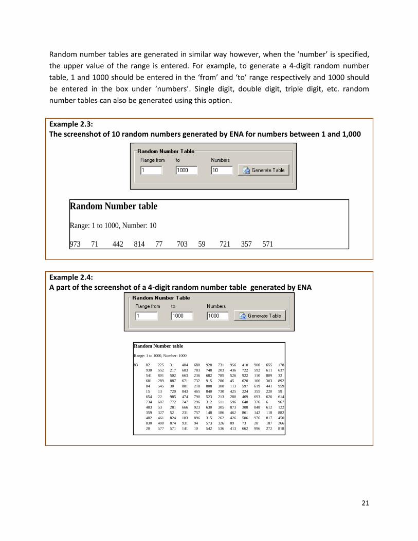
Random number tables are generated in similar way however, when the ‘number’ is specified,

the upper value of the range is entered. For example, to generate a 4-digit random number

table, 1 and 1000 should be entered in the ‘from’ and ‘to’ range respectively and 1000 should

be entered in the box under ‘numbers’. Single digit, double digit, triple digit, etc. random

number tables can also be generated using this option.

Example 2.3: The screenshot of 10 random numbers generated by ENA for numbers between 1 and 1,000

Example 2.4: A part of the screenshot of a 4-digit random number table generated by ENA

Random Number table

Range: 1 to 1000, Number: 10

973 71 442 814 77 703 59 721 357 571

Random Number table

Range: 1 to 1000, Number: 1000

83 82 225 31 404 680 928 731 956 410 900 655 178

930 552 217 683 783 748 203 436 722 592 611 637

541 801 502 663 236 682 785 526 922 110 809 32

681 289 887 671 732 915 286 45 620 106 303 892

84 545 30 881 218 808 300 113 597 619 441 959

15 13 720 843 465 840 730 425 224 355 220 59

654 22 985 474 790 523 213 280 469 693 626 614

734 607 772 747 296 312 511 596 640 376 6 967

483 53 281 666 923 630 305 873 308 848 612 122

359 327 52 231 757 148 186 462 861 142 118 882

482 461 824 183 896 315 262 426 506 976 817 450

830 400 874 931 94 573 326 89 73 28 187 266

20 577 571 141 10 542 536 413 662 996 272 818

22

Exercise 2.5:

Open the Excel file named ETH_1107_DessieZuria that comes with this user manual and go to

spread sheet no. 1 named planning. Copy the geographical areas and the population figure and

paste them onto the ENA software in Table for Cluster Sampling.

a) Assign 45 clusters. b) Transfer the assigned clusters to a Microsoft Excel file, and sort the column named, Cluster,

in assending order, and safe the file using the recommended file name.

Notes:________________________________________________________________________

______________________________________________________________________________

______________________________________________________________________________

______________________________________________________________________________

______________________________________________________________________________

Exercise 2.6:

Generate a 3 digit random number table.

Generate 12 random numbers between 1 and 98.

Notes:________________________________________________________________________

______________________________________________________________________________

______________________________________________________________________________

______________________________________________________________________________

______________________________________________________________________________

______________________________________________________________________________

23

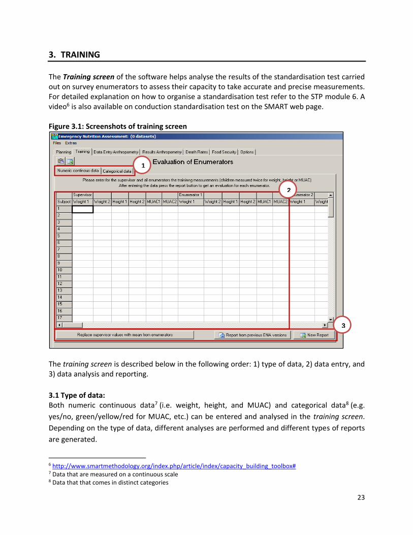
3. TRAINING The Training screen of the software helps analyse the results of the standardisation test carried out on survey enumerators to assess their capacity to take accurate and precise measurements. For detailed explanation on how to organise a standardisation test refer to the STP module 6. A video6 is also available on conduction standardisation test on the SMART web page. Figure 3.1: Screenshots of training screen

The training screen is described below in the following order: 1) type of data, 2) data entry, and 3) data analysis and reporting.

3.1 Type of data: Both numeric continuous data7 (i.e. weight, height, and MUAC) and categorical data8 (e.g.

yes/no, green/yellow/red for MUAC, etc.) can be entered and analysed in the training screen.

Depending on the type of data, different analyses are performed and different types of reports

are generated.

6 http://www.smartmethodology.org/index.php/article/index/capacity_building_toolbox# 7 Data that are measured on a continuous scale 8 Data that that comes in distinct categories

1

1

1

1

2

1

3

1

24

3.2 Data entry Data can either be entered manually or copied and pasted from a Microsoft Word or an Excel

document, which is in the same format, by selecting the <Paste> button located just above the

type of data on the training screen. Measurement values of 100 subjects from 20 enumerators

and 1 supervisor can be entered or copied and pasted at a time.

While the height and weight data are entered in 0.1 cm and 0.1 kg respectively, MUAC data

must always be entered in millimetre (mm). The software will still produce results even if a

different unit is used (e.g. cm) but the results will be wrong. The data on the training screen can

be exported to a Microsoft Excel document by clicking on the Microsoft Excel icon that is next

to the paste button on the training screen.

3.3 Data analysis and reporting For categorical data, the enumerator’s data are always compared with the supervisor’s values when analysis is performed. However, the enumerators’ numeric continuous data can be compared either with the supervisor’s values or the mean value of the enumerators by clicking on the appropriate button at the bottom of the screen (see below). For numeric continuous data, two types of reports can be generated from the software. The report that is generated by clicking the ‘Report from previous ENA versions’ is identical to the reports generated by the previous versions of ENA. The ‘New Report’ is a new feature that has been recently added to the software. The report will be generated in a Microsoft Excel format when the ‘New Report’ button is clicked. Although references are available at the end of the report, detailed guidance on how to interpret the ‘New Report’ results are not available at present. For categorical data, the report will be generated in Microsoft Word format when the Report Word button is clicked.

Important to know: In the event that only enumerators’ data are available, data can still be analysed by using the 'replace supervisor value with mean from enumerators’ button. In these situations, click on the 'replace supervisor value with mean from enumerators’ button first before the report is generated (note: as this is performed, mean values will be automatically calculated). All the reports generated after the ‘replace supervisor value with mean from enumerators’ is clicked, will only compare the individual enumerator values with the mean value of the enumerators. If the enumerator data needs to be compared again, the existing file needs to be closed and opened again.

25

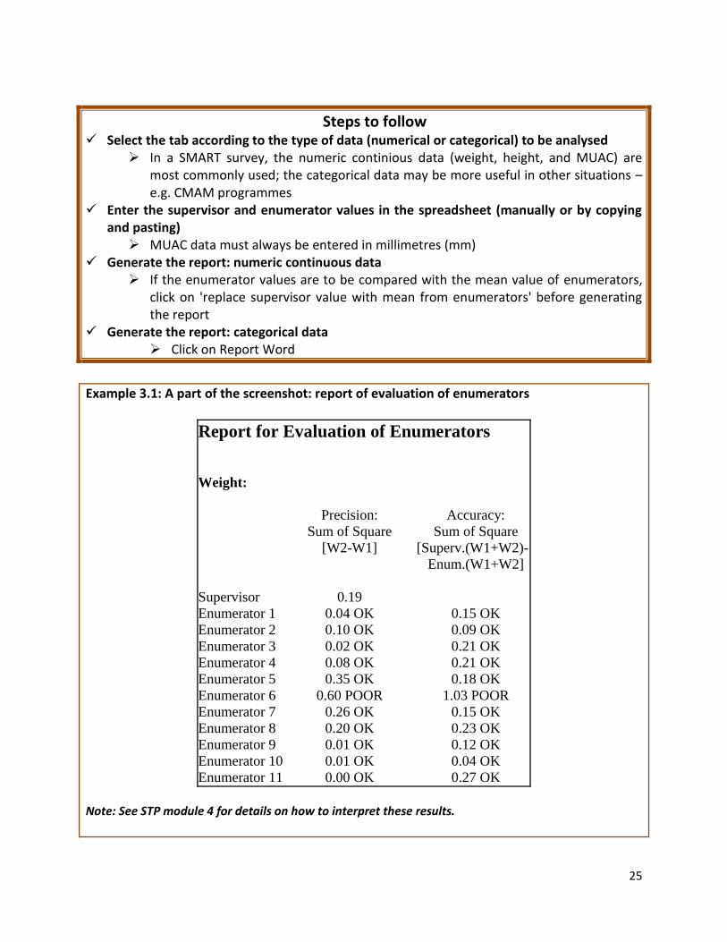
Steps to follow Select the tab according to the type of data (numerical or categorical) to be analysed

In a SMART survey, the numeric continious data (weight, height, and MUAC) are most commonly used; the categorical data may be more useful in other situations – e.g. CMAM programmes

Enter the supervisor and enumerator values in the spreadsheet (manually or by copying and pasting)

MUAC data must always be entered in millimetres (mm) Generate the report: numeric continuous data

If the enumerator values are to be compared with the mean value of enumerators, click on 'replace supervisor value with mean from enumerators' before generating the report

Generate the report: categorical data Click on Report Word

Example 3.1: A part of the screenshot: report of evaluation of enumerators

Report for Evaluation of Enumerators

Weight:

Precision: Accuracy: No. +/- No. +/-

Sum of Square Sum of Square Precision Accuracy

[W2-W1] [Superv.(W1+W2)-

Enum.(W1+W2]

Supervisor 0.19 3/1

Enumerator 1 0.04 OK 0.15 OK 2/2 4/3

Enumerator 2 0.10 OK 0.09 OK 5/2 2/5

Enumerator 3 0.02 OK 0.21 OK 1/1 3/4

Enumerator 4 0.08 OK 0.21 OK 1/4 5/2

Enumerator 5 0.35 OK 0.18 OK 6/2 3/4

Enumerator 6 0.60 POOR 1.03 POOR 6/2 7/3

Enumerator 7 0.26 OK 0.15 OK 5/2 2/4

Enumerator 8 0.20 OK 0.23 OK 4/1 3/2

Enumerator 9 0.01 OK 0.12 OK 0/1 4/2

Enumerator 10 0.01 OK 0.04 OK 1/0 4/1

Enumerator 11 0.00 OK 0.27 OK 0/0 4/4 Note: See STP module 4 for details on how to interpret these results.

26

Exercise 3.1:

Open the Excel file named ETH_1107_DessieZuria that comes with this user manual and go to

spread sheet no. 2 called training. Copy both supervisor and enumerator data and paste them

onto the Training screen. Generate the standardisation test report using the ‘report from

previous ENA versions’.

Notes:________________________________________________________________________

______________________________________________________________________________

______________________________________________________________________________

______________________________________________________________________________

______________________________________________________________________________

______________________________________________________________________________

______________________________________________________________________________

______________________________________________________________________________

______________________________________________________________________________

______________________________________________________________________________

27

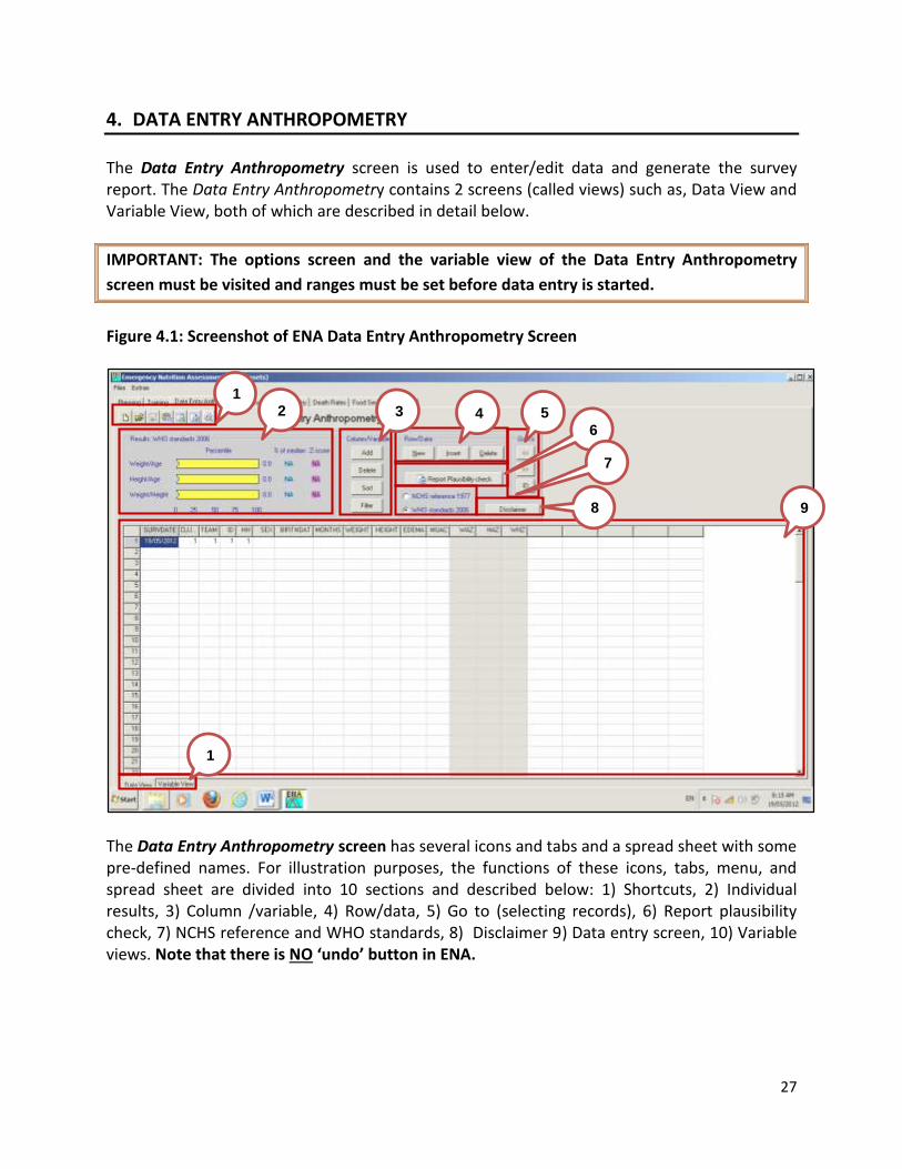
4. DATA ENTRY ANTHROPOMETRY The Data Entry Anthropometry screen is used to enter/edit data and generate the survey report. The Data Entry Anthropometry contains 2 screens (called views) such as, Data View and Variable View, both of which are described in detail below.

IMPORTANT: The options screen and the variable view of the Data Entry Anthropometry

screen must be visited and ranges must be set before data entry is started.

Figure 4.1: Screenshot of ENA Data Entry Anthropometry Screen

The Data Entry Anthropometry screen has several icons and tabs and a spread sheet with some pre-defined names. For illustration purposes, the functions of these icons, tabs, menu, and spread sheet are divided into 10 sections and described below: 1) Shortcuts, 2) Individual results, 3) Column /variable, 4) Row/data, 5) Go to (selecting records), 6) Report plausibility check, 7) NCHS reference and WHO standards, 8) Disclaimer 9) Data entry screen, 10) Variable views. Note that there is NO ‘undo’ button in ENA.

1

9

1

0

3 4 6

5

8

7

2

28

4.1 Shortcuts

Note that the first 3 icon (New, Open survey, and Save) are the same as the first 3 commands in the file menu. There are similar commands in the extras menu for the other 4 icons (see section 1.3.2 for details). Table 4.1: Functions of shortcut icons in the data entry anthropometry screen

Icon Command Function

New survey Opens a new file in .as format

Open survey Opens an existing .as file

Save survey Saves the actual.as file

Paste data from clipboard Pastes last copied data being worked on

Transfer data to excel Opens data in Microsoft Excel format as .txt file (see section 1.3.1 for details)

Report word Generates sample survey report in Microsoft Word format as .txt file (see section 1.3.1 for details)

Statistical calculator Allows further analysis and cross-tabulation of variables (see section on Results Anthropometry)

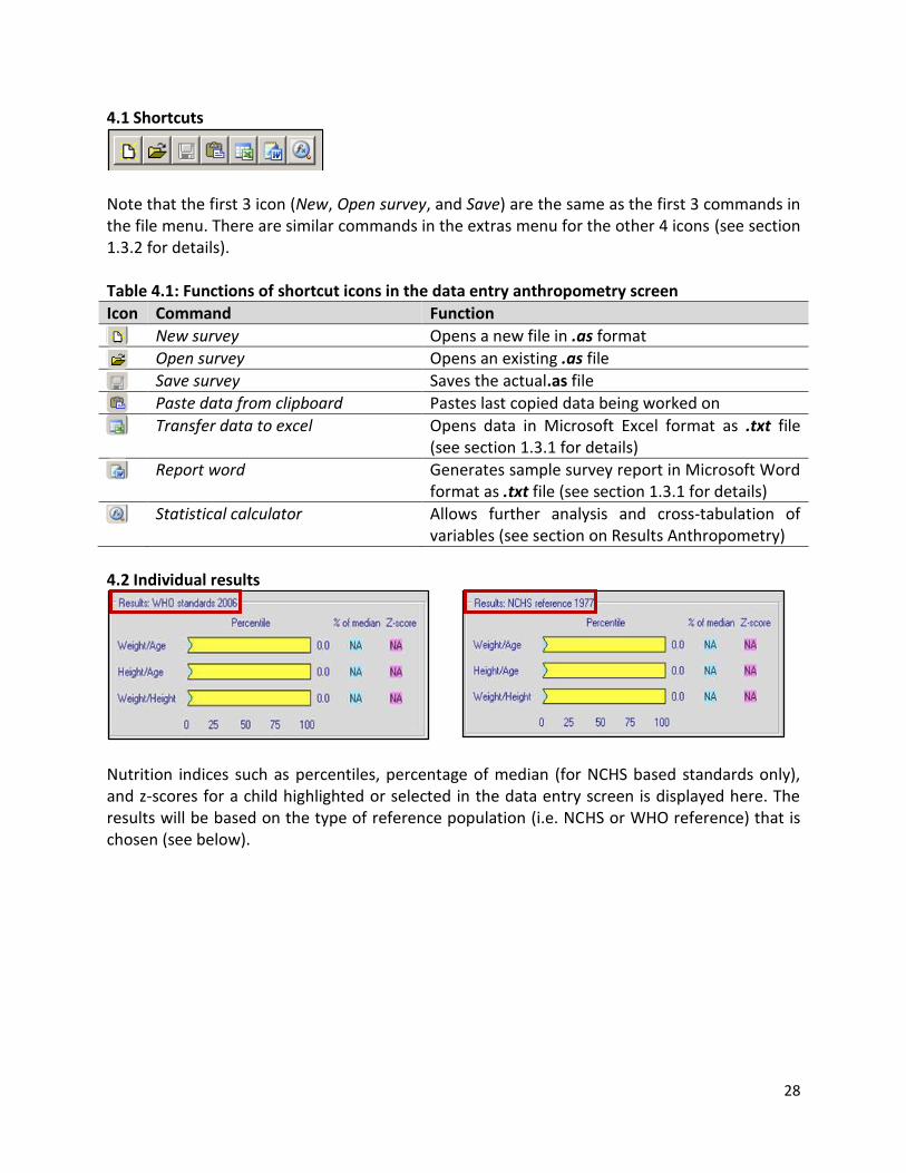
4.2 Individual results

Nutrition indices such as percentiles, percentage of median (for NCHS based standards only), and z-scores for a child highlighted or selected in the data entry screen is displayed here. The results will be based on the type of reference population (i.e. NCHS or WHO reference) that is chosen (see below).

29

4.3 Column variable Table 1.2: Functionalities of commands in the Extras menu

Function Steps to follow

Add: Includes a new variable column9

Highlight any cell after the 19th column and click on <Add>. A box will appear. Enter the name of the extra column that should be entered (e.g. Measles). Click on <OK> or <Enter>.

Delete: deletes the highlighted column10

Highlight any of the columns with a newly created variable that needs to be deleted and click on <Delete>. A box will appear asking for confirmation. Click on <Yes> or <Enter>.

Sort: Sort a variable in an ascending or descending order

Click on <Sort>. A box will appear requesting to specify the name of the variable to be sorted. Specify the variable and click on <Yes> or <Enter>.

Filter: filters selected variables based on the conditions specified

Click on <Filter>. A box will appear asking you to define the variable and the condition for filtering. Select the variable and condition (range) and click <OK>. This procedure can be repeated to filter already filtered variables and results. Click on the icon <Original file> to return to the full dataset.

4.4 Row/Data

Function Steps to follow

Add: adds a new row at the end of the dataset

Click on <Add>.

Insert: adds a new row in between rows

Highlight the cell before which a new row needs to be added and click on <Insert>.

Delete: deletes an entire row Highlight the row to be deleted and click on <delete>.

4.5 Go To (Selecting records)

Function Steps to follow

<<: Brings to the first row (ID No. 1) of the column that’s highlighted

Click on <<. The first row of the highlighted column will be displayed

>>: Brings to the last row (last subject) of the column that’s highlighted

Click on >>. The last row of the highlighted column will be displayed

ID: Brings to the ID specified Click on <ID>. A box will appear requesting the ID. Enter the ID of the record and press <OK>.

4.6 Report plausibility check report

Click on the ‘Report plausibility check’ button will

generate the plausibility check report that will open up

in a Microsoft Word format. It is essential that the

option screen is set accordingly before the plausibility check is generated – see options screen

below for details. 9 The first 19 columns are predefined and a new column variable cannot be added in between; a new column variable can only be added as the 20th columns 10 The first 19 columns are predefined and cannot be deleted; only the newly added columns can be deleted

30

4.7 NCHS reference and WHO standards This function allows the calculation of nutrition indices against both

NCHS reference and WHO standards. As the required reference is

chosen by clicking on the respective reference, the indices will be

calculated and displayed.

4.8 Disclaimer For WHO standards, a disclaimer has been included. Click on the

button to get additional details, which will disappear when the

disclaimer button is clicked on again.

4.9 Data entry screen

The data entry screen, designed as a spread sheet with columns and rows, helps enter data into the software. The first 19 columns are predefined and cannot be changed. In a default setting only 15 of the 19 columns are visible. The small check box next to the ‘showing columns for measure, cloths, and weighing variables’ in the options screen needs to be checked if all the 19 columns need to be visible on the data entry anthropometry screen (see section 7.4 for more details). Additional variables can be added and data can be entered into the software by following the procedure described above in section 4.3. Note that although any additional data can be entered, only anthropometric and death rate survey data are automatically analysed and included in the report. Additional data however can be analysed in the ENA-EPI INFO hybrid version of the software (see ‘ENA for EPI INFO user manual’ for details).

31

As the anthropometric data are entered, nutrition indices such as percentiles, z-scores, and percentage of median (for NCHS references) are automatically calculated and displayed based on the reference selected. Any data that is beyond the limit of the values set in the variable view (see below) will be displayed as flags with the cell highlighted in pink colour.

IMPORTANT:

The software recognises the difference between data from simple random survey and cluster

survey by using the numbers entered in the column, ‘cluster’. In cluster surveys, the column

‘cluster’ will have different numbers for different clusters but in simple random surveys, there

will be only one number, 1.

4.10 Variable view

The variable view is used to define the accepted values for variables in the data view. There are

3 types of variables that are defined in the software such as numeric, character and date.

Although ranges and accepted values can be set for all 3 types of variables, the software does

not recognise the range set for dates. As a result, date, even if they are outside the range set in

the variable view, will not be flagged in the data view.

All the 19 variables which are predefined in the software have default values. While most of

these default values can be changed (e.g. months, weight, height, etc.) some of them cannot be

changed (e.g. sex, cloths, measure, etc.). Each pre-defined range that could be changed should

be looked at in the context of the survey and changed accordingly. To change a pre-defined

32

value, click on the value, delete the pre-defined value using the <Delete> Key in the computer

keyboard, and enter the new value.

To ensure quality of data, it is recommended that limits are set for all additional variables

entered in the data view.

Steps to follow Follow the procedure in 4.3 and create a variable from the data view.

o Once the variable is created in the data view, it will automatically appear in the variable view

Specify the type of the value (i.e. date, numeric, or character) Enter the low range and high range

IMPORTANT: It may be required to switch between data view and variable view a few times

before the software incorporate changes and/or additions and reflects it in the data view as

flags.

Additional options for data entry from Extras menu

Some additional commands are available under the extras menu to help facilitate the data

entry and quality check process. Each of this command is described below.

Check of double entry

The ‘check of double entry’ command helps examine if there are differences between two files which have been entered independently – for example, whether the same data entered by 2 different individuals varies.

To check double entry: click on the <Extras> menu and select <Check of double entry>. A box will appear asking to specify the 2 files that need to be checked. Note that the box will open with the default folder (ena2011) selected; if the files are saved in another directory, the correct path for the file needs to be selected. Select the file and click on <OK>. A Microsoft Word document will open. If there are no discrepancies between the 2 files, the Word document will indicate so. If there are discrepancies, the Word document will provide details.

33

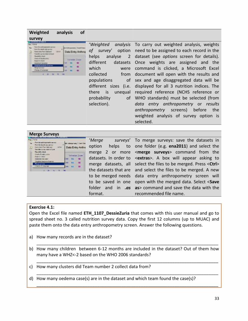
Weighted analysis of survey

‘Weighted analysis of survey’ option helps analyse 2 different datasets which were collected from populations of different sizes (i.e. there is unequal probability of selection).

To carry out weighted analysis, weights need to be assigned to each record in the dataset (see options screen for details). Once weights are assigned and the command is clicked, a Microsoft Excel document will open with the results and sex and age disaggregated data will be displayed for all 3 nutrition indices. The required reference (NCHS reference or WHO standards) must be selected (from data entry anthropometry or results anthropometry screens) before the weighted analysis of survey option is selected.

Merge Surveys

‘Merge surveys’ option helps to merge 2 or more datasets. In order to merge datasets, all the datasets that are to be merged needs to be saved in one folder and in .as format.

To merge surveys: save the datasets in one folder (e.g. ena2011) and select the <merge surveys> command from the <extras>. A box will appear asking to select the files to be merged. Press <Ctrl> and select the files to be merged. A new data entry anthropometry screen will open with the merged data. Select <Save as> command and save the data with the recommended file name.

Exercise 4.1: Open the Excel file named ETH_1107_DessieZuria that comes with this user manual and go to spread sheet no. 3 called nutrition survey data. Copy the first 12 columns (up to MUAC) and paste them onto the data entry anthropometry screen. Answer the following questions. a) How many records are in the dataset?

___________________________________________________________________________ b) How many children between 6-12 months are included in the dataset? Out of them how

many have a WHZ<-2 based on the WHO 2006 standards? ___________________________________________________________________________

c) How many clusters did Team number 2 collect data from? ___________________________________________________________________________

d) How many oedema case(s) are in the dataset and which team found the case(s)? ___________________________________________________________________________

34

e) How many record(s) are flagged? Why is(are) the data flagged? With what reference the data is/are flagged? ___________________________________________________________________________

f) What are the lowest and highest readings of MUAC? ___________________________________________________________________________

g) What is the age range in the dataset? ___________________________________________________________________________

h) Add a new column for CHILD IN PROGRAMME ___________________________________________________________________________

i) Save the file in the recommended file name format ___________________________________________________________________________

Notes: ________________________________________________________________________

______________________________________________________________________________

______________________________________________________________________________

______________________________________________________________________________

______________________________________________________________________________

______________________________________________________________________________

______________________________________________________________________________

______________________________________________________________________________

______________________________________________________________________________

______________________________________________________________________________

______________________________________________________________________________

______________________________________________________________________________

______________________________________________________________________________

______________________________________________________________________________

______________________________________________________________________________

______________________________________________________________________________

______________________________________________________________________________

35

5. RESULTS ANTHROPOMETRY The Results Anthropometry screen of the software displays the results of the anthropometric data based on nutrition indices, internationally agreed cut-offs, theoretical distributions, and different exclusion criteria. The results are depicted in diagrams and graphs (which can be copied onto the clipboard and pasted onto reports and other documents) as well as actual numbers. Nutrition indices can be further disaggregated into various categories such as sex, cluster, age, etc. The results can be obtained based on WHO standards or NCHS reference by selecting the appropriate options. The results anthropometry also enables users to produce a sample report.

IMPORTANT: The options screen must be visited and the limits must be set under Reports section of the Options screen before any anthropometric data analysis is carried out.

Figure 5.1: Screenshot of a Results Anthropometry screen

The left hand side of the screen displays the results of the survey data graphically and the right

hand side of the screen show the results numerically. The bottom of the screen is used to

specify different criteria that are used to derive the results. For illustration purposes, the entire

results anthropometry screen is divided into 6 sections and numbered, and briefly described

1 2

3 4

5

6

36

below. Examples of different graphs that can be generated from the results anthropometry

screen are then provided and discussed.

The results anthropometry section allows obtaining results against both NCHS reference and

WHO standards (by selecting the appropriate reference population in box no. 6). The results

can also be attained based on SMART flags, WHO flags, or without exclusion of any data (select

the appropriate option in the box no. 4).

Once the reference population is chosen and the required flag criterion is applied, results can

be obtained for all the 3 nutrition indices and MUAC (by selecting the necessary index or MUAC

in the box no. 3). Nutrition indices and MUAC can be further segregated by other factors such

as sex, cluster, and age (using the options in the box no. 3) as well as other options in the

dropdown menu (shown with Gaussian curve on display in box no. 5) such as Gaussian (normal)

curve, cumulative distribution, and probability plot. Additionally, when the nutrition indices are

analysed by cluster, the dropdown menu will provide further options for various distributions

such as distribution of SAM, GAM, Oedema, etc.

Based on the options specified above, the results will be displayed graphically (see box no. 1)

and numerically (see box no. 2). The graphical results can be copied using the <Clipboard>

command (see box no. 5). Clicking on the <Report Word> will generate a sample report

template with anthropometric and death rate survey results automatically filled into standard

tables (if death rate survey data is included in the file). The report will open in Microsoft Word.

Steps to follow Go to Options screen and specify the criteria for report

o E.g. Specify whether age or height should be used as the criteria for selecting records for analysis/report

o E.g. Check the MUAC cutoff and make changes as necessary Choose the reference population Select the type of flag to be automatically excluded from the final analysis Select the nutrition index to be analysed Analyse the data by

o Selecting the appropriate categories such as All, Sex, Cluster, and Age o Selecting the type of graph from the drop down menu (if cluster is selected above,

distribution of cases can also be analysed) Copy graph to clipboard and use it in report as appropriate

The functions of the results anthropometry screen described above are explained below with

an example using an anthropometric survey dataset. Note that for illustration and practical

37

purposes, the weight-for-height index and MUAC results are explained in detail here. However,

similar results can be obtained for the other 2 indices as well.

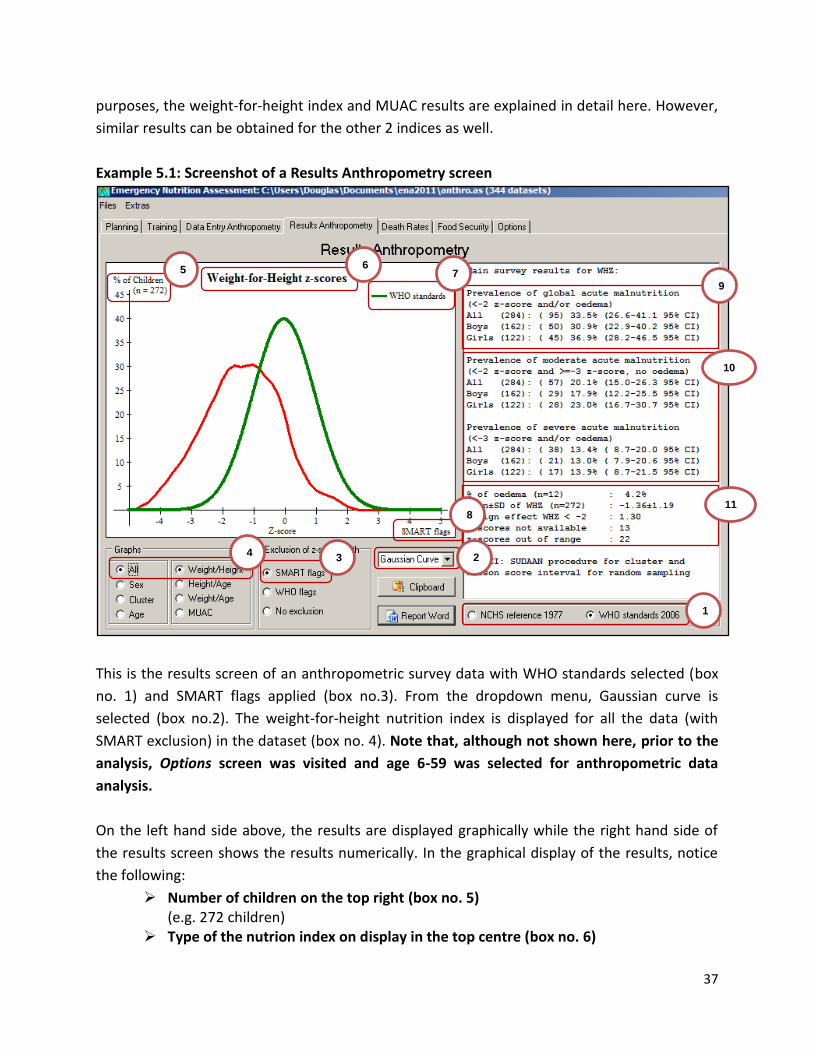
Example 5.1: Screenshot of a Results Anthropometry screen

This is the results screen of an anthropometric survey data with WHO standards selected (box

no. 1) and SMART flags applied (box no.3). From the dropdown menu, Gaussian curve is

selected (box no.2). The weight-for-height nutrition index is displayed for all the data (with

SMART exclusion) in the dataset (box no. 4). Note that, although not shown here, prior to the

analysis, Options screen was visited and age 6-59 was selected for anthropometric data

analysis.

On the left hand side above, the results are displayed graphically while the right hand side of

the results screen shows the results numerically. In the graphical display of the results, notice

the following:

Number of children on the top right (box no. 5) (e.g. 272 children)

Type of the nutrion index on display in the top centre (box no. 6)

5 6

1

1

11

9

8

3 2

1

10

7

1

4

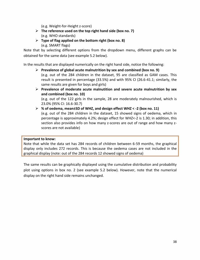
38

(e.g. Weight-for-Height z-score) The reference used on the top right hand side (box no. 7)

(e.g. WHO standards) Type of flag applied on the bottom right (box no. 8)

(e.g. SMART flags) Note that by selecting different options from the dropdown menu, different graphs can be

obtained for the same data (see example 5.2 below).

In the results that are displayed numerically on the right hand side, notice the following:

Prevalence of global acute malnutrition by sex and combined (box no. 9) (e.g. out of the 284 children in the dataset, 95 are classified as GAM cases. This result is presented in percentage (33.5%) and with 95% CI (26.6-41.1; similarly, the same results are given for boys and girls)

Prevalence of moderate acute malnutition and severe acute malnutrition by sex and combined (box no. 10) (e.g. out of the 122 girls in the sample, 28 are moderately malnourished, which is 23.0% (95% CI: 16.6-30.7)

% of oedema, mean±SD of WHZ, and design effect WHZ < -2 (box no. 11) (e.g. out of the 284 children in the dataset, 15 showed signs of oedema, which in percentage is approximately 4.2%; design effect for WHZ<-2 is 1.30; in addition, this section also provides info on how many z-scores are out of range and how many z-scores are not available)

Important to know: Note that while the data set has 284 records of children between 6-59 months, the graphical display only includes 272 records. This is because the oedema cases are not included in the graphical display (note: out of the 284 records 12 showed signs of oedema)

The same results can be graphically displayed using the cumulative distribution and probability

plot using options in box no. 2 (see example 5.2 below). However, note that the numerical

display on the right hand side remains unchanged.

39

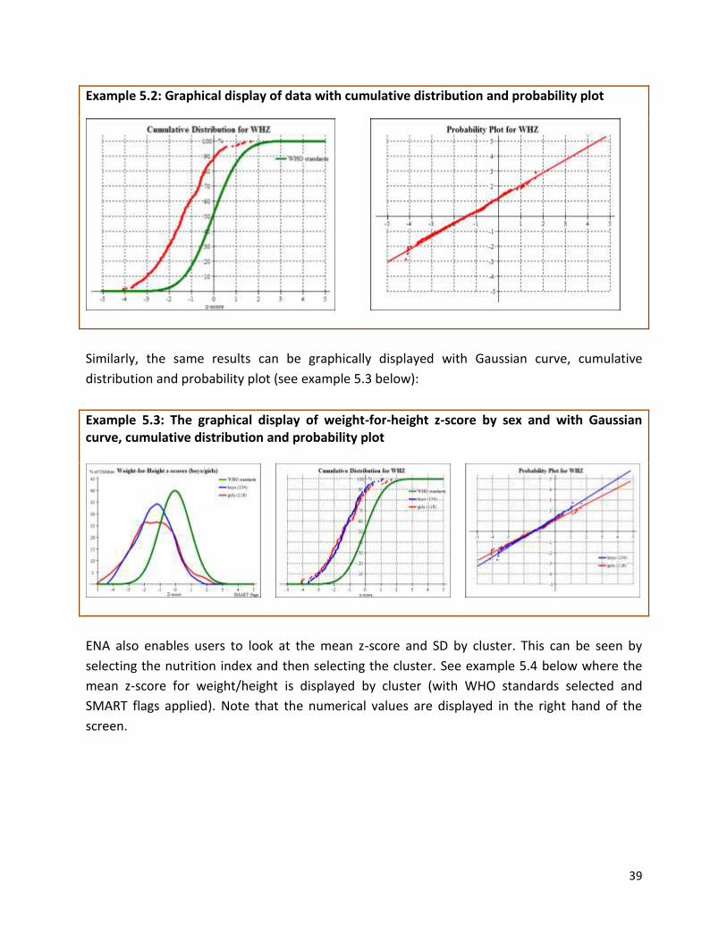
Example 5.2: Graphical display of data with cumulative distribution and probability plot

Similarly, the same results can be graphically displayed with Gaussian curve, cumulative

distribution and probability plot (see example 5.3 below):

Example 5.3: The graphical display of weight-for-height z-score by sex and with Gaussian curve, cumulative distribution and probability plot

ENA also enables users to look at the mean z-score and SD by cluster. This can be seen by

selecting the nutrition index and then selecting the cluster. See example 5.4 below where the

mean z-score for weight/height is displayed by cluster (with WHO standards selected and

SMART flags applied). Note that the numerical values are displayed in the right hand of the

screen.

40

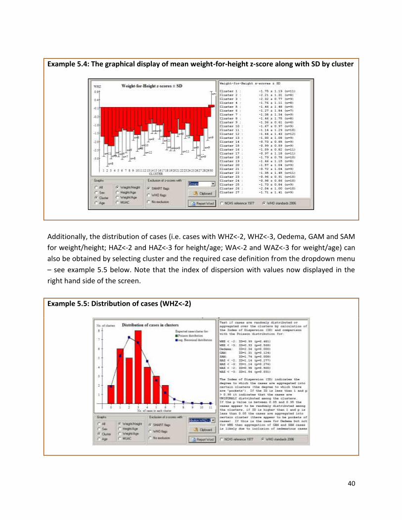
Example 5.4: The graphical display of mean weight-for-height z-score along with SD by cluster

Additionally, the distribution of cases (i.e. cases with WHZ<-2, WHZ<-3, Oedema, GAM and SAM

for weight/height; HAZ<-2 and HAZ<-3 for height/age; WA<-2 and WAZ<-3 for weight/age) can

also be obtained by selecting cluster and the required case definition from the dropdown menu

– see example 5.5 below. Note that the index of dispersion with values now displayed in the

right hand side of the screen.

Example 5.5: Distribution of cases (WHZ<-2)

41

The results (the mean z-score±SD) can also be obtained by age group by selecting the nutrition

index to be analysed along with ‘age’. See example 5.6 where weight/height z-score is displayed

by age groups. Note that the results are displayed numerically on the right hand side of the

screen.

Example 5.6: The graphical display of weight/height by age groups

MUAC is displayed graphically as cumulative curve, which can also be disaggregated by sex. See

example 5.7 below for details.

Example 5.7: Display of MUAC by age

42

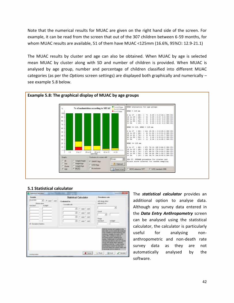
Note that the numerical results for MUAC are given on the right hand side of the screen. For

example, it can be read from the screen that out of the 307 children between 6-59 months, for

whom MUAC results are available, 51 of them have MUAC <125mm (16.6%, 95%CI: 12.9-21.1)

The MUAC results by cluster and age can also be obtained. When MUAC by age is selected

mean MUAC by cluster along with SD and number of children is provided. When MUAC is

analysed by age group, number and percentage of children classified into different MUAC

categories (as per the Options screen settings) are displayed both graphically and numerically –

see example 5.8 below.

Example 5.8: The graphical display of MUAC by age groups

5.1 Statistical calculator The statistical calculator provides an

additional option to analyse data.

Although any survey data entered in

the Data Entry Anthropometry screen

can be analysed using the statistical

calculator, the calculator is particularly

useful for analysing non-

anthropometric and non-death rate

survey data as they are not

automatically analysed by the

software.

43

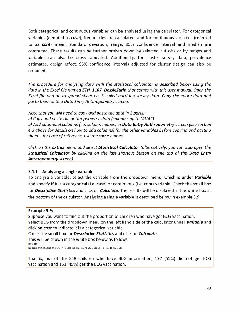
Both categorical and continuous variables can be analysed using the calculator. For categorical

variables (denoted as case), frequencies are calculated, and for continuous variables (referred

to as cont) mean, standard deviation, range, 95% confidence interval and median are

computed. These results can be further broken down by selected cut offs or by ranges and

variables can also be cross tabulated. Additionally, for cluster survey data, prevalence

estimates, design effect, 95% confidence intervals adjusted for cluster design can also be

obtained.

The procedure for analysing data with the statistical calculator is described below using the data in the Excel file named ETH_1107_DessieZuria that comes with this user manual. Open the Excel file and go to spread sheet no. 3 called nutrition survey data. Copy the entire data and paste them onto a Data Entry Anthropometry screen. Note that you will need to copy and paste the data in 2 parts: a) Copy and paste the anthropometric data (columns up to MUAC) b) Add additional columns (i.e. column names) in Data Entry Anthropometry screen (see section 4.3 above for details on how to add columns) for the other variables before copying and pasting them – for ease of reference, use the same names. Click on the Extras menu and select Statistical Calculator (alternatively, you can also open the Statistical Calculator by clicking on the last shortcut button on the top of the Data Entry Anthropometry screen).

5.1.1 Analysing a single variable To analyse a variable, select the variable from the dropdown menu, which is under Variable

and specify if it is a categorical (i.e. case) or continuous (i.e. cont) variable. Check the small box

for Descriptive Statistics and click on Calculate. The results will be displayed in the white box at

the bottom of the calculator. Analysing a single variable is described below in example 5.9

Example 5.9: Suppose you want to find out the proportion of children who have got BCG vaccination. Select BCG from the dropdown menu on the left hand side of the calculator under Variable and click on case to indicate it is a categorical variable. Check the small box for Descriptive Statistics and click on Calculate. This will be shown in the white box below as follows: Results: Descriptive statistics BCG (n=358); n] (n= 197) 55.0 %; y] (n= 161) 45.0 %; That is, out of the 358 children who have BCG information, 197 (55%) did not get BCG vaccination and 161 (45%) get the BCG vaccination.

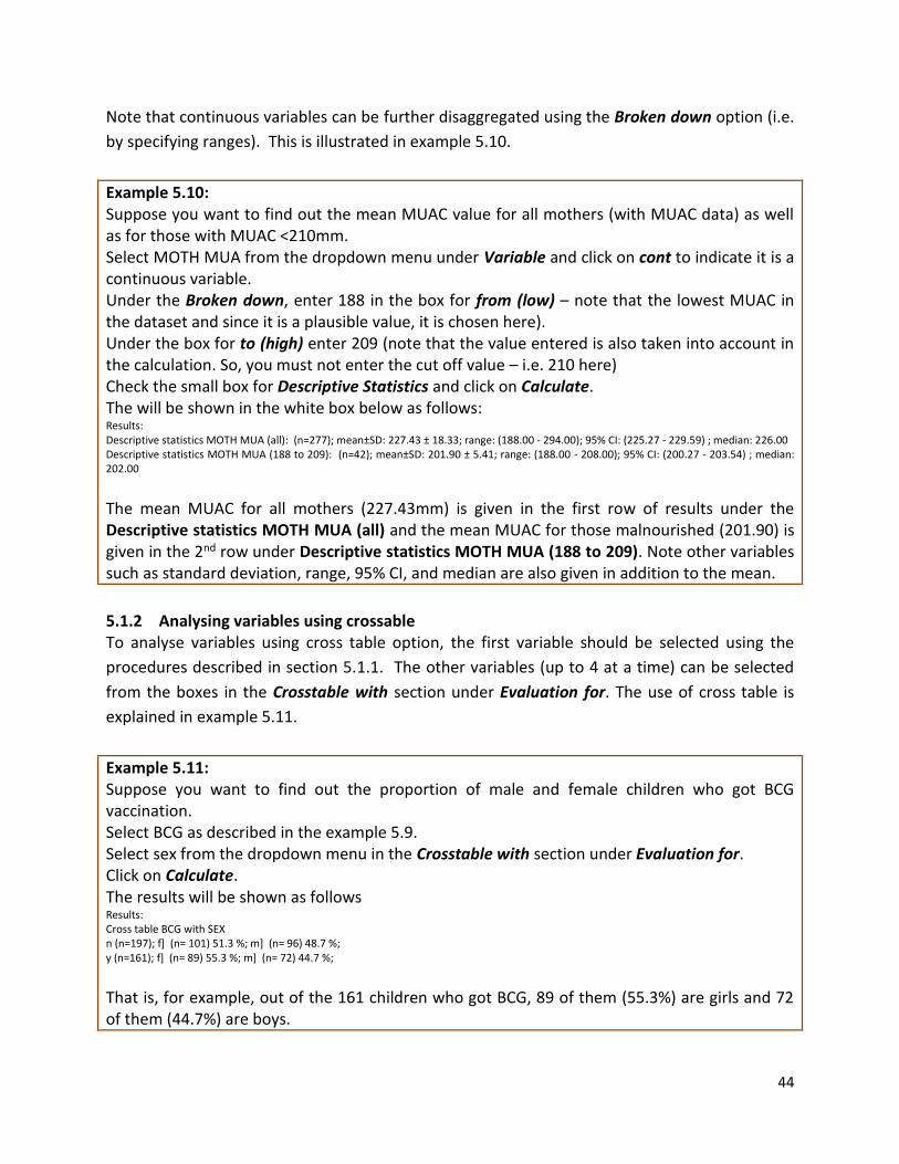
44

Note that continuous variables can be further disaggregated using the Broken down option (i.e.

by specifying ranges). This is illustrated in example 5.10.

Example 5.10: Suppose you want to find out the mean MUAC value for all mothers (with MUAC data) as well as for those with MUAC <210mm. Select MOTH MUA from the dropdown menu under Variable and click on cont to indicate it is a continuous variable. Under the Broken down, enter 188 in the box for from (low) – note that the lowest MUAC in the dataset and since it is a plausible value, it is chosen here). Under the box for to (high) enter 209 (note that the value entered is also taken into account in the calculation. So, you must not enter the cut off value – i.e. 210 here) Check the small box for Descriptive Statistics and click on Calculate. The will be shown in the white box below as follows: Results: Descriptive statistics MOTH MUA (all): (n=277); mean±SD: 227.43 ± 18.33; range: (188.00 - 294.00); 95% CI: (225.27 - 229.59) ; median: 226.00 Descriptive statistics MOTH MUA (188 to 209): (n=42); mean±SD: 201.90 ± 5.41; range: (188.00 - 208.00); 95% CI: (200.27 - 203.54) ; median: 202.00 The mean MUAC for all mothers (227.43mm) is given in the first row of results under the Descriptive statistics MOTH MUA (all) and the mean MUAC for those malnourished (201.90) is given in the 2nd row under Descriptive statistics MOTH MUA (188 to 209). Note other variables such as standard deviation, range, 95% CI, and median are also given in addition to the mean.

5.1.2 Analysing variables using crossable To analyse variables using cross table option, the first variable should be selected using the

procedures described in section 5.1.1. The other variables (up to 4 at a time) can be selected

from the boxes in the Crosstable with section under Evaluation for. The use of cross table is

explained in example 5.11.

Example 5.11: Suppose you want to find out the proportion of male and female children who got BCG vaccination. Select BCG as described in the example 5.9. Select sex from the dropdown menu in the Crosstable with section under Evaluation for. Click on Calculate. The results will be shown as follows Results: Cross table BCG with SEX n (n=197); f] (n= 101) 51.3 %; m] (n= 96) 48.7 %; y (n=161); f] (n= 89) 55.3 %; m] (n= 72) 44.7 %; That is, for example, out of the 161 children who got BCG, 89 of them (55.3%) are girls and 72 of them (44.7%) are boys.

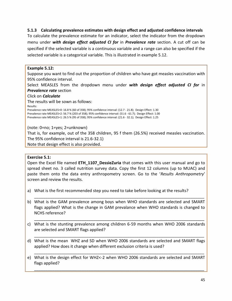
45

5.1.3 Calculating prevalence estimates with design effect and adjusted confidence intervals To calculate the prevalence estimate for an indicator, select the indicator from the dropdown

menu under with design effect adjusted CI for in Prevalence rate section. A cut off can be

specified if the selected variable is a continuous variable and a range can also be specified if the

selected variable is a categorical variable. This is illustrated in example 5.12.

Example 5.12: Suppose you want to find out the proportion of children who have got measles vaccination with 95% confidence interval. Select MEASLES from the dropdown menu under with design effect adjusted CI for in Prevalence rate section Click on Calculate The results will be sown as follows: Results: Prevalence rate MEASLES=0: 16.8 % (60 of 358); 95% confidence interval: (12.7 - 21.8); Design Effect: 1.30 Prevalence rate MEASLES=2: 56.7 % (203 of 358); 95% confidence interval: (51.6 - 61.7); Design Effect: 1.00 Prevalence rate MEASLES=1: 26.5 % (95 of 358); 95% confidence interval: (21.6 - 32.1); Design Effect: 1.25 (note: 0=no; 1=yes; 2=unknown) That is, for example, out of the 358 children, 95 f them (26.5%) received measles vaccination. The 95% confidence interval is 21.6-32.1) Note that design effect is also provided.

Exercise 5.1: Open the Excel file named ETH_1107_DessieZuria that comes with this user manual and go to spread sheet no. 3 called nutrition survey data. Copy the first 12 columns (up to MUAC) and paste them onto the data entry anthropometry screen. Go to the ‘Results Anthropometry’ screen and review the results. a) What is the first recommended step you need to take before looking at the results?

___________________________________________________________________________ b) What is the GAM prevalence among boys when WHO standards are selected and SMART

flags applied? What is the change in GAM prevalance when WHO standards is changed to NCHS reference? ___________________________________________________________________________

c) What is the stunting prevalence among children 6-59 months when WHO 2006 standards are selected and SMART flags applied? ___________________________________________________________________________

d) What is the mean WHZ and SD when WHO 2006 standards are selected and SMART flags applied? How does it change when different exclusion criteria is used? ___________________________________________________________________________

e) What is the design effect for WHZ<-2 when WHO 2006 standards are selected and SMART flags applied? ___________________________________________________________________________

46

f) What is the Index of Dispersion and p-value for oedema when WHO 2006 standards are selected and SMART flags applied? ___________________________________________________________________________

g) What is the mean WHZ and standards deviation for the age group 6-17 months when WHO 2006 standards are selected and SMART flags applied? ___________________________________________________________________________

h) Generate the sample survey report and save it using the recommended file name. ___________________________________________________________________________

Notes: ________________________________________________________________________

______________________________________________________________________________

______________________________________________________________________________

______________________________________________________________________________

______________________________________________________________________________

______________________________________________________________________________

______________________________________________________________________________

______________________________________________________________________________

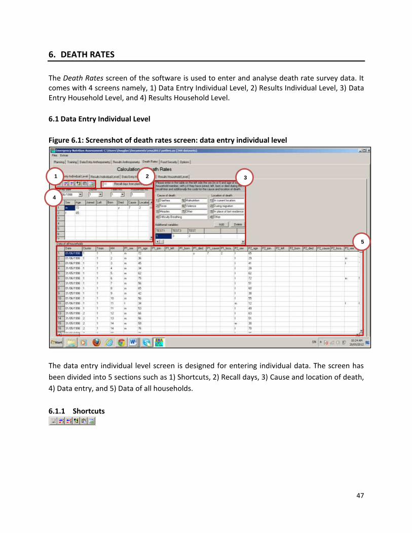
47

6. DEATH RATES

The Death Rates screen of the software is used to enter and analyse death rate survey data. It comes with 4 screens namely, 1) Data Entry Individual Level, 2) Results Individual Level, 3) Data Entry Household Level, and 4) Results Household Level.

6.1 Data Entry Individual Level

Figure 6.1: Screenshot of death rates screen: data entry individual level

The data entry individual level screen is designed for entering individual data. The screen has

been divided into 5 sections such as 1) Shortcuts, 2) Recall days, 3) Cause and location of death,

4) Data entry, and 5) Data of all households.

6.1.1 Shortcuts

1 2 3

5

4

48

Table 6.1: Functions of icons on death rates screen

Icon Command Function Steps to follow

Save survey Saves the actual file .as Click on the icon. If the data is saved for the first time, a box will appear with recommendation for file format. Save the file according to the recommended format. Once the file is created, the data will be saved automatically onto the file when this icon is clicked

Insert row A new row is added just above the highlighted cell in the data for all households section

Highlight the cell above which the row needs to be created and click on the icon.

Delete row An entire row of a highlighted cell is deleted in the data for all households section

Highlight one cell the row that needs to be deleted and click on the icon.

Takeover of HH + cluster numbers

Date, cluster, team and household and cluster numbers from data entry anthropometry screen will be copied and pasted here

Click on the icon. A box will appear asking for confirmation for copying the information from data entry anthropometry screen. Click on <OK>. The date, cluster, team and household and cluster numbers information will appear.

Paste data from clipboard

Pastes last copied data Highlight the cell on which data needs to be pasted and click on the icon. The last copied data will be pasted on the highlighted cell.

Transfer data to excel

Opens data in Microsoft Excel format

Click on the icon and the entire dataset will be transferred to Excel.

6.1.2 Recall days The figure displayed in the box named ‘recall days from

planning sheet’ on the data entry individual level screen

(and also the data entry household level screen) corresponds to the number of recall days that

was used to calculate the sample size (note that since the default setting is used in the

illustration here, the default setting of the 90 day recall period appears here but this will vary

from survey to survey. This must be decided separately for each survey based on the survey

objectives). The number of recall days cannot be entered here. If the sample size for the death

rate is not calculated in the same file that is used for entering death rate survey data or due to

any other reason where the planning screen doesn’t have the same recall period that the

survey used, it is important to change this in the planning screen.

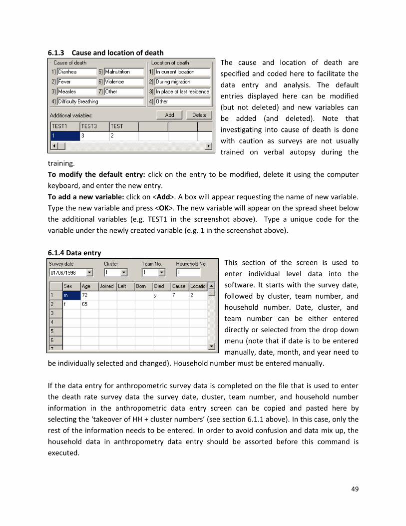
49

6.1.3 Cause and location of death The cause and location of death are

specified and coded here to facilitate the

data entry and analysis. The default

entries displayed here can be modified

(but not deleted) and new variables can

be added (and deleted). Note that

investigating into cause of death is done

with caution as surveys are not usually

trained on verbal autopsy during the

training.

To modify the default entry: click on the entry to be modified, delete it using the computer

keyboard, and enter the new entry.

To add a new variable: click on <Add>. A box will appear requesting the name of new variable.

Type the new variable and press <OK>. The new variable will appear on the spread sheet below

the additional variables (e.g. TEST1 in the screenshot above). Type a unique code for the

variable under the newly created variable (e.g. 1 in the screenshot above).

6.1.4 Data entry This section of the screen is used to

enter individual level data into the

software. It starts with the survey date,

followed by cluster, team number, and

household number. Date, cluster, and

team number can be either entered

directly or selected from the drop down

menu (note that if date is to be entered

manually, date, month, and year need to

be individually selected and changed). Household number must be entered manually.

If the data entry for anthropometric survey data is completed on the file that is used to enter

the death rate survey data the survey date, cluster, team number, and household number

information in the anthropometric data entry screen can be copied and pasted here by

selecting the ‘takeover of HH + cluster numbers’ (see section 6.1.1 above). In this case, only the

rest of the information needs to be entered. In order to avoid confusion and data mix up, the

household data in anthropometry data entry should be assorted before this command is

executed.

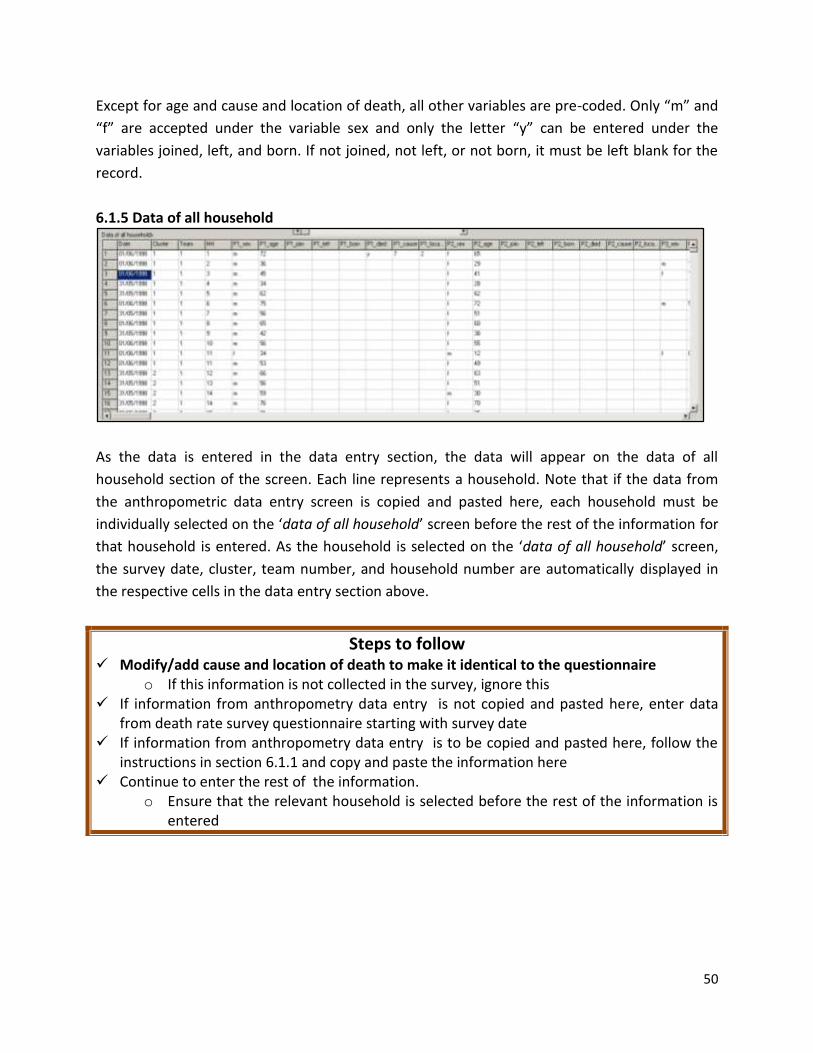
50

Except for age and cause and location of death, all other variables are pre-coded. Only “m” and

“f” are accepted under the variable sex and only the letter “y” can be entered under the

variables joined, left, and born. If not joined, not left, or not born, it must be left blank for the

record.

6.1.5 Data of all household

As the data is entered in the data entry section, the data will appear on the data of all

household section of the screen. Each line represents a household. Note that if the data from

the anthropometric data entry screen is copied and pasted here, each household must be

individually selected on the ‘data of all household’ screen before the rest of the information for

that household is entered. As the household is selected on the ‘data of all household’ screen,

the survey date, cluster, team number, and household number are automatically displayed in

the respective cells in the data entry section above.

Steps to follow Modify/add cause and location of death to make it identical to the questionnaire

o If this information is not collected in the survey, ignore this If information from anthropometry data entry is not copied and pasted here, enter data

from death rate survey questionnaire starting with survey date If information from anthropometry data entry is to be copied and pasted here, follow the

instructions in section 6.1.1 and copy and paste the information here Continue to enter the rest of the information.

o Ensure that the relevant household is selected before the rest of the information is entered

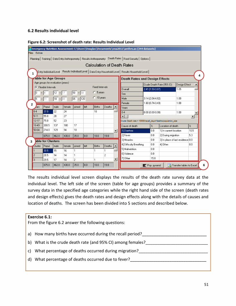
51

6.2 Results individual level

Figure 6.2: Screenshot of death rate: Results Individual Level

The results individual level screen displays the results of the death rate survey data at the

individual level. The left side of the screen (table for age groups) provides a summary of the

survey data in the specified age categories while the right hand side of the screen (death rates

and design effects) gives the death rates and design effects along with the details of causes and

location of deaths. The screen has been divided into 5 sections and described below.

Exercise 6.1: From the figure 6.2 answer the following questions: a) How many births have occurred during the recall period?____________________________

b) What is the crude death rate (and 95% CI) among females?___________________________

c) What percentage of deaths occurred during migration?______________________________

d) What percentage of deaths occurred due to fever?_________________________________

1

2

3

4

6

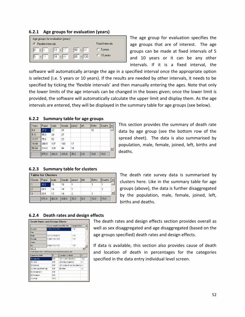
52

6.2.1 Age groups for evaluation (years) The age group for evaluation specifies the

age groups that are of interest. The age

groups can be made at fixed intervals of 5

and 10 years or it can be any other

intervals. If it is a fixed interval, the

software will automatically arrange the age in a specified interval once the appropriate option

is selected (i.e. 5 years or 10 years). If the results are needed by other intervals, it needs to be

specified by ticking the ‘flexible intervals’ and then manually entering the ages. Note that only

the lower limits of the age intervals can be changed in the boxes given; once the lower limit is

provided, the software will automatically calculate the upper limit and display them. As the age

intervals are entered, they will be displayed in the summary table for age groups (see below).

6.2.2 Summary table for age groups This section provides the summary of death rate

data by age group (see the bottom row of the

spread sheet). The data is also summarised by

population, male, female, joined, left, births and

deaths.

6.2.3 Summary table for clusters The death rate survey data is summarised by

clusters here. Like in the summary table for age

groups (above), the data is further disaggregated

by the population, male, female, joined, left,

births and deaths.

6.2.4 Death rates and design effects The death rates and design effects section provides overall as

well as sex disaggregated and age disaggregated (based on the

age groups specified) death rates and design effects.

If data is available, this section also provides cause of death

and location of death in percentages for the categories

specified in the data entry individual level screen.

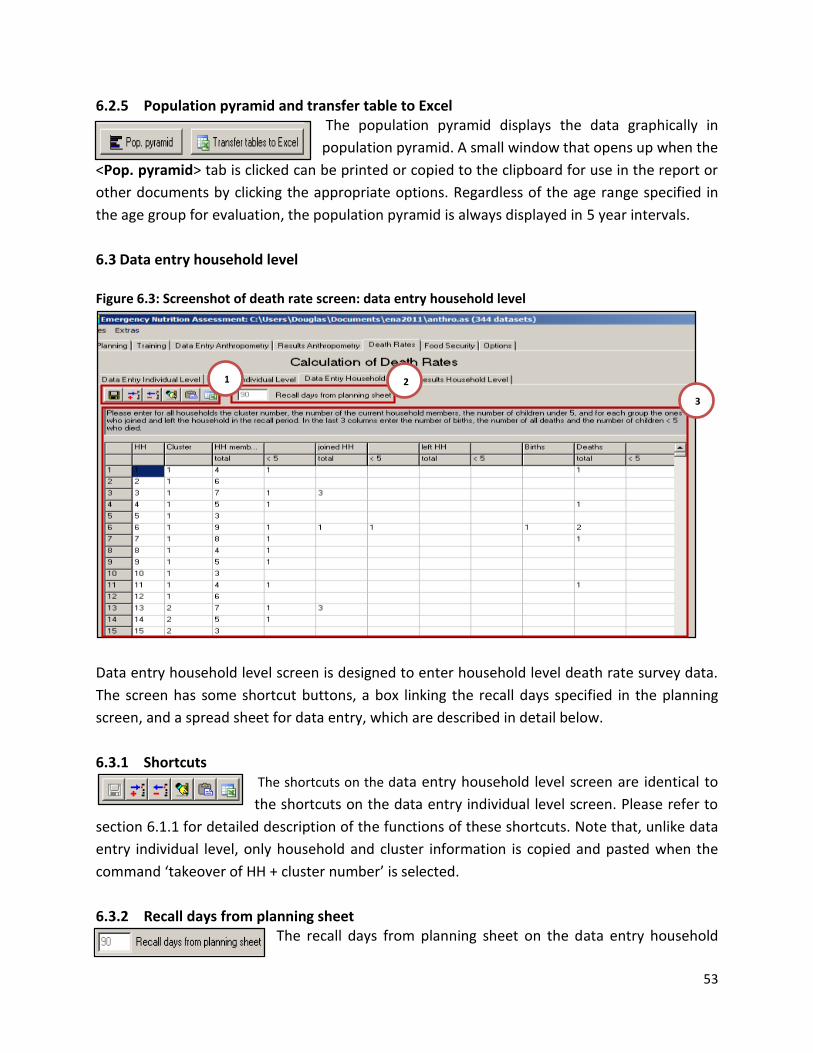
53

6.2.5 Population pyramid and transfer table to Excel The population pyramid displays the data graphically in

population pyramid. A small window that opens up when the

<Pop. pyramid> tab is clicked can be printed or copied to the clipboard for use in the report or

other documents by clicking the appropriate options. Regardless of the age range specified in

the age group for evaluation, the population pyramid is always displayed in 5 year intervals.

6.3 Data entry household level

Figure 6.3: Screenshot of death rate screen: data entry household level

Data entry household level screen is designed to enter household level death rate survey data.

The screen has some shortcut buttons, a box linking the recall days specified in the planning

screen, and a spread sheet for data entry, which are described in detail below.

6.3.1 Shortcuts The shortcuts on the data entry household level screen are identical to

the shortcuts on the data entry individual level screen. Please refer to

section 6.1.1 for detailed description of the functions of these shortcuts. Note that, unlike data

entry individual level, only household and cluster information is copied and pasted when the

command ‘takeover of HH + cluster number’ is selected.

6.3.2 Recall days from planning sheet The recall days from planning sheet on the data entry household

1 2

3

54

level screen is identical to the recall days from planning sheet on the data entry individual level

screen. Please refer to section 6.1.2 for detailed description.

6.3.3 Spread sheet for data entry The spread sheet is used to enter household level death rate survey

data. The summary data for households are entered starting with

the household number. The data is disaggregated by only one

criterion, age (under 5 years and over 5 years).

Steps to follow If information from anthropometry data entry is not copied and pasted here, enter data

from death rate survey questionnaire starting with household number o Note that only household and cluster number from anthropometry data will be

pasted If information from anthropometry data entry is to be copied and pasted here, follow the

instructions in section 6.1.1 and copy and paste the information

Notes: ________________________________________________________________________

______________________________________________________________________________

______________________________________________________________________________

______________________________________________________________________________

______________________________________________________________________________

______________________________________________________________________________

______________________________________________________________________________

______________________________________________________________________________

______________________________________________________________________________

______________________________________________________________________________

______________________________________________________________________________

______________________________________________________________________________

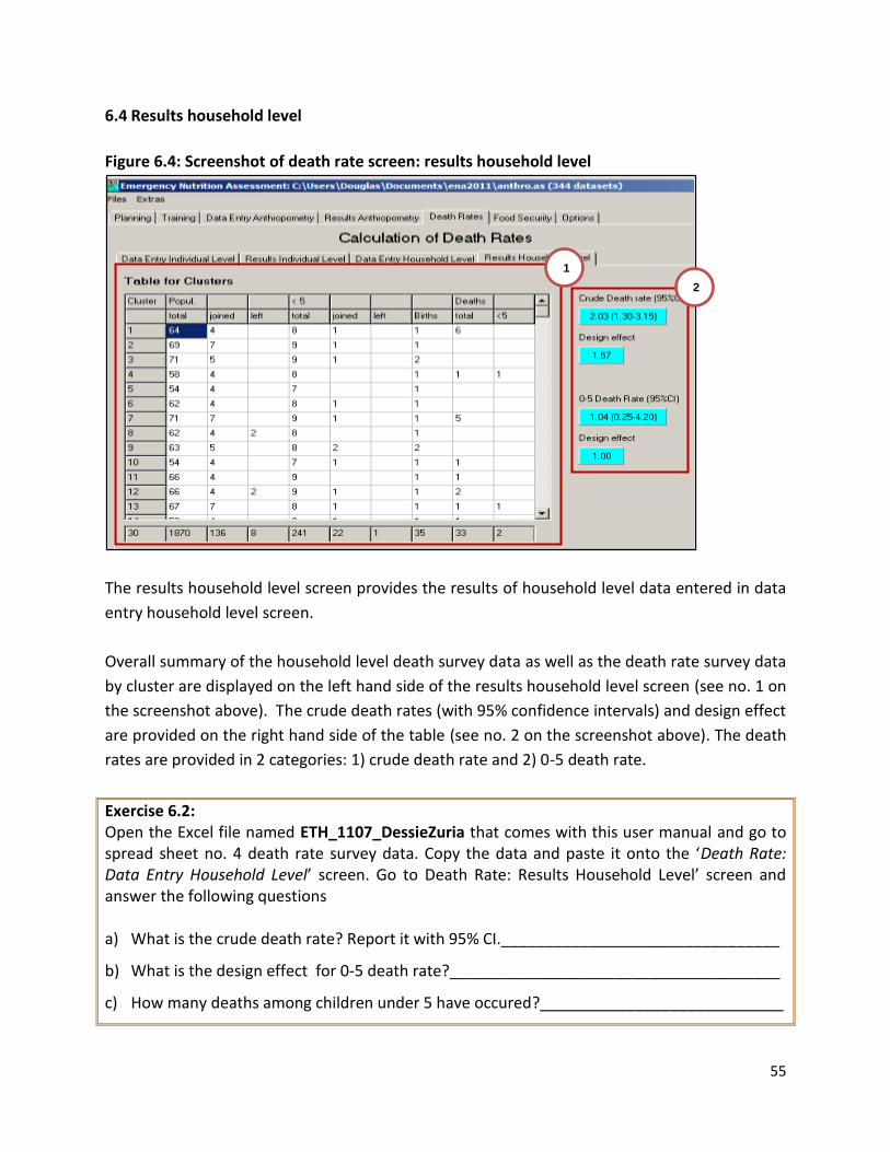
55

6.4 Results household level

Figure 6.4: Screenshot of death rate screen: results household level

The results household level screen provides the results of household level data entered in data

entry household level screen.

Overall summary of the household level death survey data as well as the death rate survey data

by cluster are displayed on the left hand side of the results household level screen (see no. 1 on

the screenshot above). The crude death rates (with 95% confidence intervals) and design effect

are provided on the right hand side of the table (see no. 2 on the screenshot above). The death

rates are provided in 2 categories: 1) crude death rate and 2) 0-5 death rate.

Exercise 6.2: Open the Excel file named ETH_1107_DessieZuria that comes with this user manual and go to spread sheet no. 4 death rate survey data. Copy the data and paste it onto the ‘Death Rate: Data Entry Household Level’ screen. Go to Death Rate: Results Household Level’ screen and answer the following questions a) What is the crude death rate? Report it with 95% CI.________________________________

b) What is the design effect for 0-5 death rate?______________________________________

c) How many deaths among children under 5 have occured?____________________________

1

2

56

Notes: ________________________________________________________________________

______________________________________________________________________________

______________________________________________________________________________

______________________________________________________________________________

______________________________________________________________________________

______________________________________________________________________________

______________________________________________________________________________

______________________________________________________________________________

______________________________________________________________________________

______________________________________________________________________________

______________________________________________________________________________

______________________________________________________________________________

______________________________________________________________________________

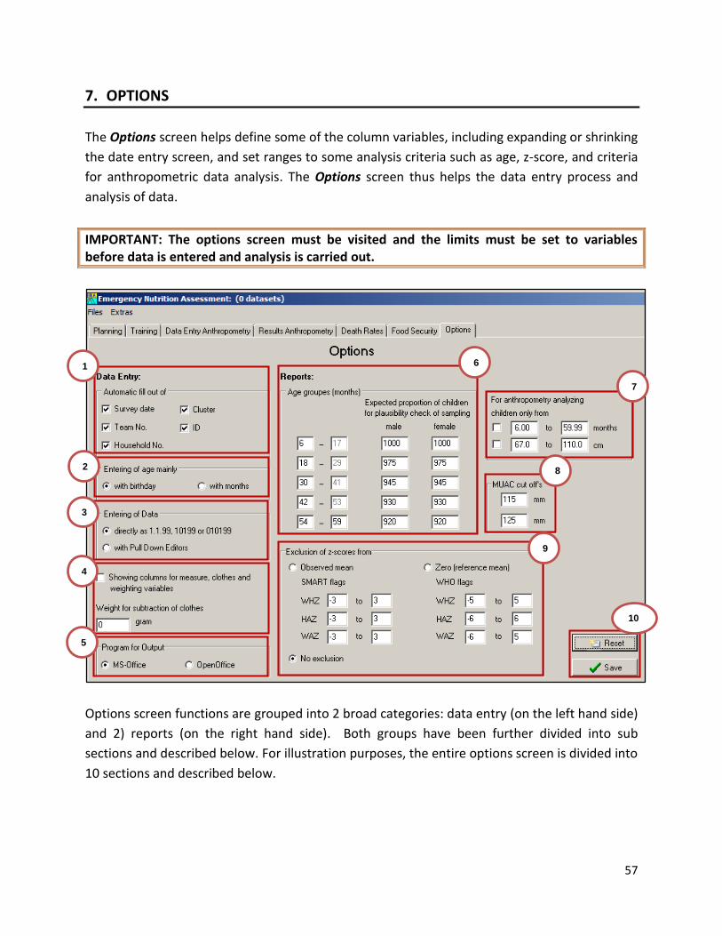
57

7. OPTIONS

The Options screen helps define some of the column variables, including expanding or shrinking

the date entry screen, and set ranges to some analysis criteria such as age, z-score, and criteria

for anthropometric data analysis. The Options screen thus helps the data entry process and

analysis of data.

IMPORTANT: The options screen must be visited and the limits must be set to variables before data is entered and analysis is carried out.

Options screen functions are grouped into 2 broad categories: data entry (on the left hand side)

and 2) reports (on the right hand side). Both groups have been further divided into sub

sections and described below. For illustration purposes, the entire options screen is divided into

10 sections and described below.

1

2

3

4

5

6

7

8

9

10

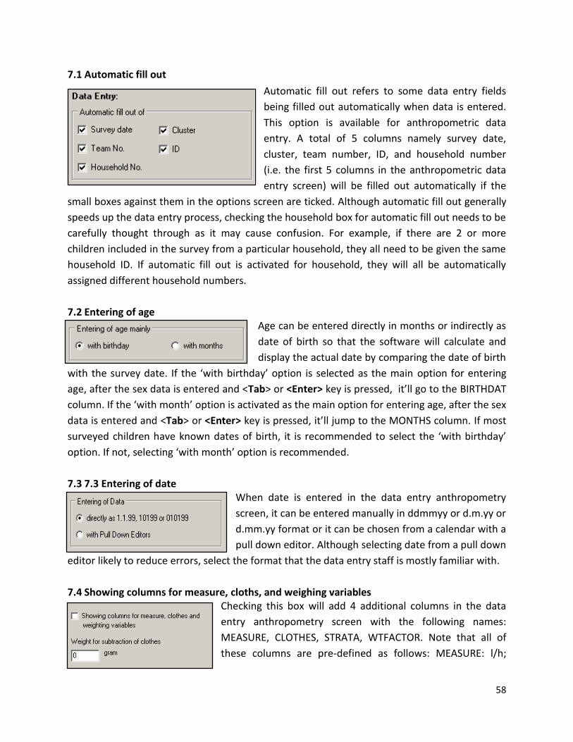
58

7.1 Automatic fill out

Automatic fill out refers to some data entry fields

being filled out automatically when data is entered.

This option is available for anthropometric data

entry. A total of 5 columns namely survey date,

cluster, team number, ID, and household number

(i.e. the first 5 columns in the anthropometric data

entry screen) will be filled out automatically if the

small boxes against them in the options screen are ticked. Although automatic fill out generally

speeds up the data entry process, checking the household box for automatic fill out needs to be

carefully thought through as it may cause confusion. For example, if there are 2 or more

children included in the survey from a particular household, they all need to be given the same

household ID. If automatic fill out is activated for household, they will all be automatically

assigned different household numbers.

7.2 Entering of age Age can be entered directly in months or indirectly as

date of birth so that the software will calculate and

display the actual date by comparing the date of birth

with the survey date. If the ‘with birthday’ option is selected as the main option for entering

age, after the sex data is entered and <Tab> or <Enter> key is pressed, it’ll go to the BIRTHDAT

column. If the ‘with month’ option is activated as the main option for entering age, after the sex

data is entered and <Tab> or <Enter> key is pressed, it’ll jump to the MONTHS column. If most

surveyed children have known dates of birth, it is recommended to select the ‘with birthday’

option. If not, selecting ‘with month’ option is recommended.

7.3 7.3 Entering of date When date is entered in the data entry anthropometry

screen, it can be entered manually in ddmmyy or d.m.yy or

d.mm.yy format or it can be chosen from a calendar with a

pull down editor. Although selecting date from a pull down

editor likely to reduce errors, select the format that the data entry staff is mostly familiar with.

7.4 Showing columns for measure, cloths, and weighing variables Checking this box will add 4 additional columns in the data

entry anthropometry screen with the following names:

MEASURE, CLOTHES, STRATA, WTFACTOR. Note that all of

these columns are pre-defined as follows: MEASURE: l/h;

59

CLOTHES: y/n; and STRATA and WTFACTOR: numeric value with optional decimal separator.

MEASURE: according to the protocol, length should be measured (lying down position) for all

children below the age of 2 and height measurement (standing up position) should be made for

older children. If for any unavoidable circumstances, the only length measurement could be

taken on a child who is older than 2 years or only height measurement could be possible on a

child who is less than 2 years of age, the enumerators should do the measurement accordingly

and make a special note on the questionnaire. Note that if height is used as admission criteria,

87 cm will be the deciding point – i.e. length measurement on all children below 87 cm and

height measurement on children more than 87 cm should be taken. If children less than 87cm

were measured standing up or children more than 87 cm were measured lying down,

enumerators should make a special note on the questionnaire.

When these cases are entered into the software, these should be specified so that the software

will apply a correction factor and correct nutrition indices accordingly. If a child that is supposed

to be measured lying down (e.g. 13 month old child) is measured standing up, under the

MEASURE column, the letter ‘h’ (meaning ‘height’) should be entered. Similarly, if a child that is

supposed to be measured standing up (e.g. 33 month old child) is measured lying down, under

the MEASURE column, the letter ‘l’ (meaning ‘length’) should be entered.

CLOTHES: Children should be weighed naked. If for any reason it is not possible to measure

them naked, they should be weighed with clothes and the approximate weight of clothes

should be taken and noted on the questionnaire.

Before the data entry, the average weight of clothes should be entered in the space provided

under the ‘weight for subtraction of clothes’ in the options screen in grams. When the data of

children who were weighed with clothes are entered, the letter ‘y’ (meaning yes) should be

entered into the CLOTHES column for these children. The software will subtract the weight of

the clothes from the total weight entered for the child before calculating nutrition indices. For

those children who were measured without clothes, it is not necessary to enter the letter ‘n’

(meaning no) in the column, CLOTHES.

STRATA: STRATA refers to stratification. In certain surveys, the entire population is divided into

different strata (sub-groups) before sampling is carried out. In these surveys, stratification also

needs to be taken into account when data is analysed. The column STRATA is included for this

purpose. However, its functionality is still being tested at present and therefore no further

guidance is given as to how to use this functionality.

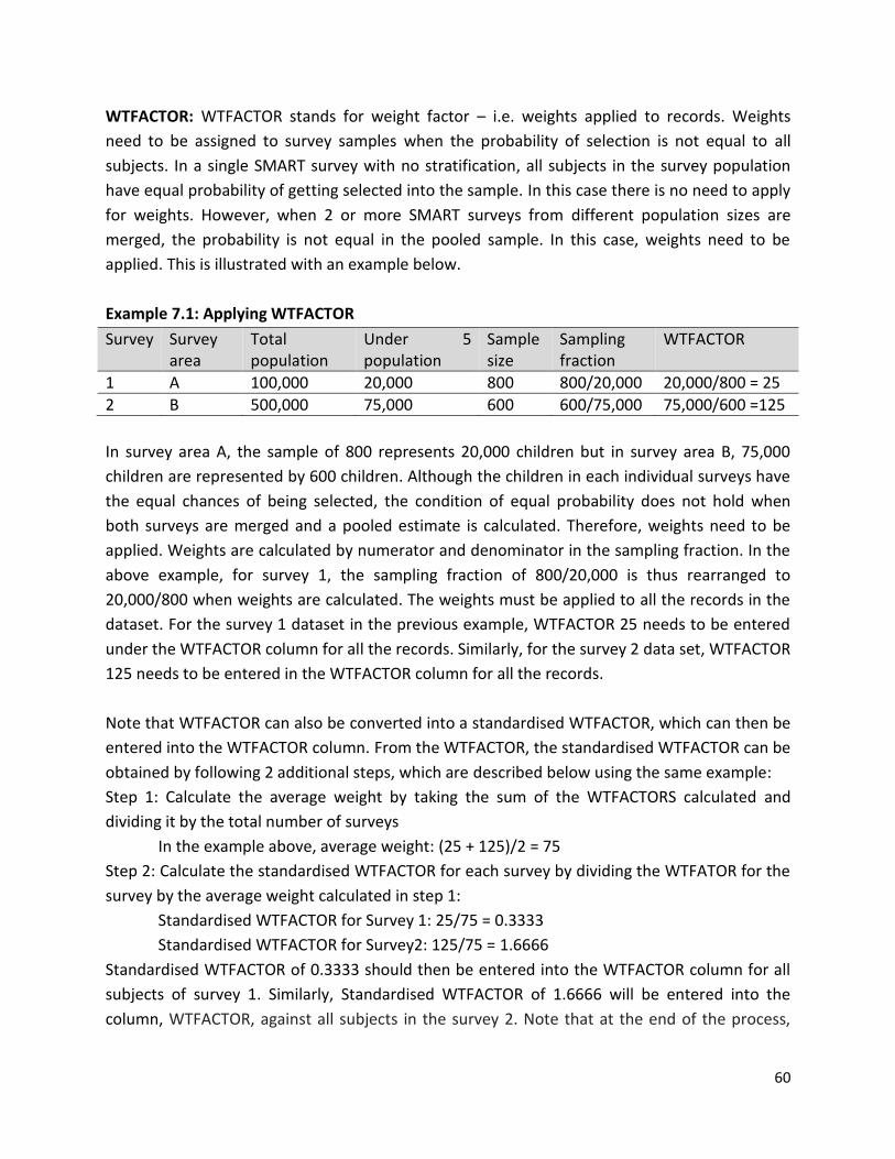
60

WTFACTOR: WTFACTOR stands for weight factor – i.e. weights applied to records. Weights

need to be assigned to survey samples when the probability of selection is not equal to all

subjects. In a single SMART survey with no stratification, all subjects in the survey population

have equal probability of getting selected into the sample. In this case there is no need to apply

for weights. However, when 2 or more SMART surveys from different population sizes are

merged, the probability is not equal in the pooled sample. In this case, weights need to be

applied. This is illustrated with an example below.

Example 7.1: Applying WTFACTOR

Survey Survey area

Total population

Under 5 population

Sample size

Sampling fraction

WTFACTOR

1 A 100,000 20,000 800 800/20,000 20,000/800 = 25

2 B 500,000 75,000 600 600/75,000 75,000/600 =125

In survey area A, the sample of 800 represents 20,000 children but in survey area B, 75,000

children are represented by 600 children. Although the children in each individual surveys have

the equal chances of being selected, the condition of equal probability does not hold when

both surveys are merged and a pooled estimate is calculated. Therefore, weights need to be

applied. Weights are calculated by numerator and denominator in the sampling fraction. In the

above example, for survey 1, the sampling fraction of 800/20,000 is thus rearranged to

20,000/800 when weights are calculated. The weights must be applied to all the records in the

dataset. For the survey 1 dataset in the previous example, WTFACTOR 25 needs to be entered

under the WTFACTOR column for all the records. Similarly, for the survey 2 data set, WTFACTOR

125 needs to be entered in the WTFACTOR column for all the records.

Note that WTFACTOR can also be converted into a standardised WTFACTOR, which can then be

entered into the WTFACTOR column. From the WTFACTOR, the standardised WTFACTOR can be

obtained by following 2 additional steps, which are described below using the same example:

Step 1: Calculate the average weight by taking the sum of the WTFACTORS calculated and

dividing it by the total number of surveys

In the example above, average weight: (25 + 125)/2 = 75

Step 2: Calculate the standardised WTFACTOR for each survey by dividing the WTFATOR for the

survey by the average weight calculated in step 1:

Standardised WTFACTOR for Survey 1: 25/75 = 0.3333

Standardised WTFACTOR for Survey2: 125/75 = 1.6666

Standardised WTFACTOR of 0.3333 should then be entered into the WTFACTOR column for all

subjects of survey 1. Similarly, Standardised WTFACTOR of 1.6666 will be entered into the

column, WTFACTOR, against all subjects in the survey 2. Note that at the end of the process,

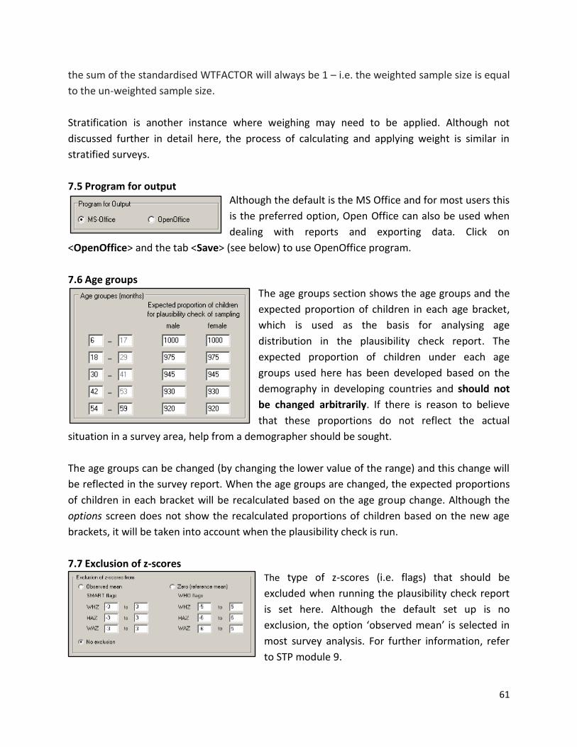
61

the sum of the standardised WTFACTOR will always be 1 – i.e. the weighted sample size is equal

to the un-weighted sample size.

Stratification is another instance where weighing may need to be applied. Although not

discussed further in detail here, the process of calculating and applying weight is similar in

stratified surveys.

7.5 Program for output Although the default is the MS Office and for most users this

is the preferred option, Open Office can also be used when

dealing with reports and exporting data. Click on

<OpenOffice> and the tab <Save> (see below) to use OpenOffice program.

7.6 Age groups The age groups section shows the age groups and the

expected proportion of children in each age bracket,

which is used as the basis for analysing age

distribution in the plausibility check report. The

expected proportion of children under each age

groups used here has been developed based on the

demography in developing countries and should not

be changed arbitrarily. If there is reason to believe

that these proportions do not reflect the actual

situation in a survey area, help from a demographer should be sought.

The age groups can be changed (by changing the lower value of the range) and this change will

be reflected in the survey report. When the age groups are changed, the expected proportions

of children in each bracket will be recalculated based on the age group change. Although the

options screen does not show the recalculated proportions of children based on the new age

brackets, it will be taken into account when the plausibility check is run.

7.7 Exclusion of z-scores The type of z-scores (i.e. flags) that should be

excluded when running the plausibility check report

is set here. Although the default set up is no

exclusion, the option ‘observed mean’ is selected in

most survey analysis. For further information, refer

to STP module 9.

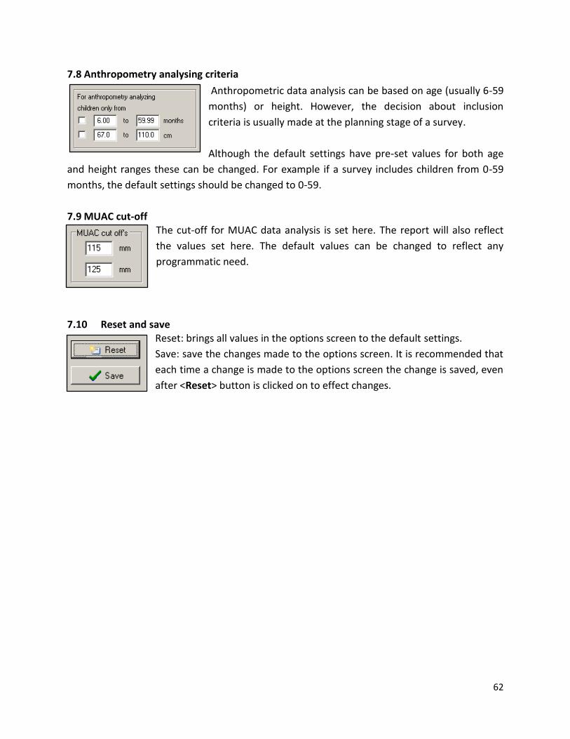
62

7.8 Anthropometry analysing criteria

Anthropometric data analysis can be based on age (usually 6-59

months) or height. However, the decision about inclusion

criteria is usually made at the planning stage of a survey.

Although the default settings have pre-set values for both age

and height ranges these can be changed. For example if a survey includes children from 0-59

months, the default settings should be changed to 0-59.

7.9 MUAC cut-off The cut-off for MUAC data analysis is set here. The report will also reflect

the values set here. The default values can be changed to reflect any

programmatic need.

7.10 Reset and save Reset: brings all values in the options screen to the default settings.

Save: save the changes made to the options screen. It is recommended that

each time a change is made to the options screen the change is saved, even

after <Reset> button is clicked on to effect changes.

63

Annex 1: Death Rate Survey Form

FSAU/FAO SOMALIA: MODIFIED MORTALITY SURVEY QUESTIONNAIRE

Enumerator’s Name:__________________ Team No: _____________ Date: ______________

Household No: _________ Cluster No: ________ District: ______________ Village: ____________

No. 1: Name 2: Sex 3: Age (yrs)

4: Born since _____ (insert the start of the recall period)

5: Arrived since _____ (insert the start of the recall period)

6: Cause of death

7: Location of death

a) How many members are present in this household now? List them.

b) How many members have left this household (out migrants) since _____ (insert the start of the recall period)? List them

c) Do you have any member of the household who has died since _____ (insert the start of the recall period)? List them

Summary

U5 Total

Current HH Members

Arrivals during the Recall period

Number who have left during Recall period

Births during recall

Deaths during recall period

64

Annex 2: Converting sample size from children to households

𝑵𝒖𝒎𝒃𝒆𝒓 𝒐𝒇 𝒉𝒐𝒖𝒔𝒆𝒉𝒐𝒍𝒅𝒔 𝒕𝒐 𝒃𝒆 𝒗𝒊𝒔𝒊𝒕𝒆𝒅 =𝑺𝒂𝒎𝒑𝒍𝒆 𝒔𝒊𝒛𝒆 𝒄𝒂𝒍𝒄𝒖𝒍𝒂𝒕𝒆𝒅 𝒊𝒏 𝒏𝒐. 𝒐𝒇 𝒄𝒉𝒊𝒍𝒅𝒓𝒆𝒏 𝟔−𝟓𝟗

𝑨𝒗𝒆𝒓𝒂𝒈𝒆 𝒉𝒐𝒖𝒔𝒆𝒉𝒐𝒍𝒅 𝒔𝒊𝒛𝒆 𝒙 𝒑𝒆𝒓𝒄𝒆𝒏𝒕𝒂𝒈𝒆 𝒐𝒇 𝒄𝒉𝒊𝒍𝒅𝒓𝒆𝒏 𝒖𝒏𝒅𝒆𝒓 𝟓 𝑿 𝟎.𝟗

Example:

When the sample size for an anthropometric survey among children between 6-59 months was

calculated in ENA, a sample size of 483 children was obtained. Convert the number of children

into households. According to the recent DHS survey, the average household size in the survey

area is 5.5 and percentage of children under five is 18%.

Answer:

Note that Sample size in children 6-59 months can be converted into households by applying

required figures directly in the formula above. For illustration purposes, however, the answer is

shown in multiple steps below.

Step 1: Calculate the average under 5 children per household by multiplying the average

household size by the % of children under five

Average under 5 children per household = Average household size x % of children under 5

= 5.5 x 18/100

= 0.99

(This means that each household has 0.99 under 5 children; in other words, if you visit 100

households you will get approximately 99 children)

Step 2: Calculate the average number of children between 6-59 months per household by

multiplying average under 5 children by 0.9

Note that the under 5 population can be broken down into 10 equal parts of 6-month brackets

(i.e. 0-5, 6-12, 13-18 … 44-50) and children 6-59 month includes 9 of these age brackets (i.e.

9/10=0.9). Assuming that the proportion of children in each of these age bracket is the same,

the under 5 population is multiplied by 0.9 to obtain the total number of children 6-59 months.

Similarly, multiplying the under 5 population by 0.4 would give the approximate number of

children under 2.

Average number of children between 6-59 months per HH = average under 5 children x 0.9

= 0.99 x 0.9

= 0.891

(This means that each household has 0.891 children 6-59 months; in other words, if you visit 100

households you will get approximately 89 children6-59 months)

65

Step 3: Calculate the number of households to be visited by dividing the sample size by the

average number of children between 6-59 months per household

Total no. of HH = Total sample size of children 6-59/Average no. of children 6-59 per HH

= 483/0.891

= 542

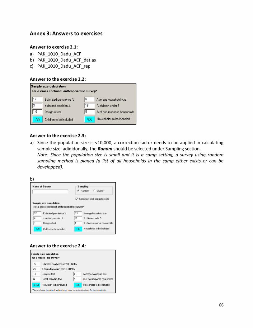
66

Annex 3: Answers to exercises

Answer to exercise 2.1:

a) PAK_1010_Dadu_ACF b) PAK_1010_Dadu_ACF_dat.as c) PAK_1010_Dadu_ACF_rep

Answer to the exercise 2.2:

Answer to the exercise 2.3:

a) Since the population size is <10,000, a correction factor needs to be applied in calculating sample size. adididonally, the Ranom should be selected under Sampling section. Note: Since the population size is small and it is a camp setting, a survey using random sampling method is planed (a list of all households in the camp either exists or can be developped).

b)

Answer to the exercise 2.4:

67

Answer to exercise 2.5:

a) The table for cluster sampling in the Planning screen should look like the fllowing once the geographical units are copied and pasted onto the, the number of clusters specified as 45 and the ‘Assign Custer’ button is clicked:

b) The Microsoft Excel file, whch contain the transferred data, should look like the following once the Clusters are sorted (note that the clusters selected will vary as the first village is selected randomly):

The file should be named as ETH_1107_DessieZuria_AssignedClusters_xls

Geographical unit Population size Cluster

Yebiso 290 1

Ayata 1 576 2

Mayan mamedo 1 683 3

Alekodayo 643 4

Berara tuwate tsehay 871 5

Genfot 1 437 6

Jerjero 2 535 7

Meyane 1 533 8

Golbo 624 9

Kermemie 662 10

Guassa 1 677 11

Weltu 2 521 12

Temsase 518 13

Gobeya 709 14

Erkoche 861 15

Werebecho 779 16

Tidegebeya 2 786 17

Jimetit 724 18

Jema 732 19

Wereruga 301 20

Eshetie Ager 556 21

Kurach Ager 1 559 22

Abaweldiye 414 23

Tigaja 766 24

Doyo Ager 376 25

Matebo 668 26

Yegof 842 27

Chorka Mender 2 526 28

Abachufa 486 29

Abecho 733 30

Kurkur 495 31

Jegolasitaya 890 32

Gobeya 799 33

Mendebona feto 816 34

Gena Memcha 476 35

Abiagerna Betoager 595 36

Dedibona Geferssa 738 37

Tach kelad 600 38

Enessana 799 39

Goshign 671 40

Bikeru 552 41

Amboasa 442 42

Tatessa 590 43

Endulti 581 44

Gero 728 45

Buko Ager 666 RC

Neftegna 486 RC

Yinale 614 RC

Sereser 457 RC

Kilkilo 528 RC

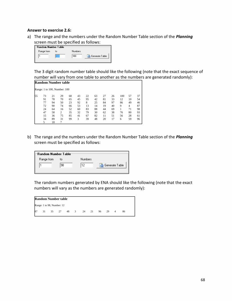
68

Answer to exercise 2.6:

a) The range and the numbers under the Random Number Table section of the Planning screen must be specified as follows:

The 3 digit random number table should like the following (note that the exact sequence of number will vary from one table to another as the numbers are generated randomly):

b) The range and the numbers under the Random Number Table section of the Planning screen must be specified as follows:

The random numbers generated by ENA should like the following (note that the exact numbers will vary as the numbers are generated randomly):

Random Number table

Range: 1 to 100, Number: 100

55 73 21 29 68 43 22 63 27 26 100 57 37

91 78 70 65 45 95 42 81 33 12 10 54

77 94 50 23 92 8 25 84 97 86 49 46

72 90 74 66 53 13 14 19 40 9 4 87

24 64 16 52 60 83 88 44 69 1 71 98

47 58 2 35 32 79 30 62 38 76 80 93

15 36 75 85 41 67 82 11 51 56 28 61

34 89 31 99 3 39 48 20 17 6 59 96

5 18 7

Random Number table

Range: 1 to 98, Number: 12

87 31 35 27 48 3 24 21 96 29 4 86

69

Answer to exercise 3.1:

Once the data is copied and pasted, the ENA training screen should look like the following:

The output should be like the following when the report from previous ENA versions button is

clicked (note that only part of the output is displayed here):

Answer to exercise 4.1:

a) 359 b) Children between 6-12 months included in the dataset = 41; number of children 6-12

months who have WHZ<-2=2 a WHZ<-2? c) 7 (cluster numbers: 9, 17, 31, 34, 38, 41, and 44) d) 1; team no 2 e) 1; The particular reacord is flagged because it’s is outside of the SMART flag range (the

mean value for WHZ is -0.86 so, any WHZ value ±3 of the mean value will be flagged as abnormal). The data is flagged when WHO standards are selected and SMART flags applied.

f) Lowest reading of MUAC = 96 mm; Highest readings of MUAC = 170 mm g) 6-59 months

h) The column heading should appear something like this: i) ETH_1107_DessieZuria_data.as

Report for Evaluation of Enumerators

Weight:

Precision: Accuracy: No. +/- No. +/-

Sum of Square Sum of Square Precision Accuracy

[W2-W1] [Superv.(W1+W2)-

Enum.(W1+W2]

Supervisor 0.19 3/1

Enumerator 1 0.04 OK 0.15 OK 2/2 4/3

Enumerator 2 0.10 OK 0.09 OK 5/2 2/5

Enumerator 3 0.02 OK 0.21 OK 1/1 3/4

Enumerator 4 0.08 OK 0.21 OK 1/4 5/2

Enumerator 5 0.35 OK 0.18 OK 6/2 3/4

Enumerator 6 0.60 POOR 1.03 POOR 6/2 7/3

Enumerator 7 0.26 OK 0.15 OK 5/2 2/4

Enumerator 8 0.20 OK 0.23 OK 4/1 3/2

Enumerator 9 0.01 OK 0.12 OK 0/1 4/2

Enumerator 10 0.01 OK 0.04 OK 1/0 4/1

Enumerator 11 0.00 OK 0.27 OK 0/0 4/4

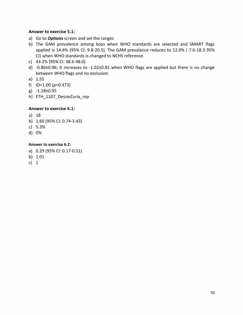
70

Answer to exercise 5.1:

a) Go to Options screen and set the ranges b) The GAM prevalence among boys when WHO standards are selected and SMART flags

applied is 14.4% (95% CI: 9.8-20.5). The GAM prevalance reduces to 12.0% ( 7.6-18.3 95% CI) when WHO standards is changed to NCHS reference.

c) 43.2% (95% CI: 38.6-48.0) d) -0.86±0.96; It increases to -1.02±0.81 when WHO flags are applied but there is no change

between WHO flags and no exclusion. e) 1.55 f) ID=1.00 (p=0.473) g) -1.18±0.95 h) ETH_1107_DessieZuria_rep

Answer to exercise 6.1:

a) 18 b) 1.60 (95% CI: 0.74-3.43) c) 5.3% d) 0%

Answer to exercise 6.2:

a) 0.29 (95% CI: 0.17-0.51) b) 1.01 c) 1