Embodied carbon in trade: a survey of the empirical literature · Embodied carbon in trade: A...

Embodied carbon in trade: a survey of the

empirical literature!

Misato Sato!April 2012!

Centre for Climate Change Economics and Policy Working Paper No. 89!

Grantham Research Institute on Climate Change and the Environment

Working Paper No. 77!

The Centre for Climate Change Economics and Policy (CCCEP) was established by the University of Leeds and the London School of Economics and Political Science in 2008 to advance public and private action on climate change through innovative, rigorous research. The Centre is funded by the UK Economic and Social Research Council and has five inter-linked research programmes:

1. Developing climate science and economics 2. Climate change governance for a new global deal 3. Adaptation to climate change and human development 4. Governments, markets and climate change mitigation 5. The Munich Re Programme - Evaluating the economics of climate risks and

opportunities in the insurance sector More information about the Centre for Climate Change Economics and Policy can be found at: http://www.cccep.ac.uk. The Grantham Research Institute on Climate Change and the Environment was established by the London School of Economics and Political Science in 2008 to bring together international expertise on economics, finance, geography, the environment, international development and political economy to create a world-leading centre for policy-relevant research and training in climate change and the environment. The Institute is funded by the Grantham Foundation for the Protection of the Environment, and has five research programmes:

1. Global response strategies 2. Green growth 3. Practical aspects of climate policy 4. Adaptation and development 5. Resource security

More information about the Grantham Research Institute on Climate Change and the Environment can be found at: http://www.lse.ac.uk/grantham. This working paper is intended to stimulate discussion within the research community and among users of research, and its content may have been submitted for publication in academic journals. It has been reviewed by at least one internal referee before publication. The views expressed in this paper represent those of the author(s) and do not necessarily represent those of the host institutions or funders.

Embodied carbon in trade: A survey of the empiricalliterature⇤

Misato Sato†

Abstract

This paper critically reviews the literature on embodied carbon in trade and evaluatesour present empirical understanding of these flows. A careful comparison of quantitativeresults from this literature exposes significant inconsistencies. For instance, estimates foremission embodied in world trade in 2004 range between 4.4 Gt and 6.2 Gt CO2, thedifference corresponding to around half of Europe’s annual emissions. A few consistentthemes do nevertheless emerge from the literature. Most importantly, emissions in tradeconstitute a large and growing share of global emissions. Uncertainty about country-level embodied emissions remains large, however, which presents severe limitations forthe practical application of embodied carbon principles in climate policy.

1 Introduction

To what extent do trade and consumption contribute to rising global greenhouse gas (GHG)emissions? Will strengthening domestic climate policy measures lead to real reductions inGHG emissions or relocation of industry and emissions to countries with lax regulation?Who is responsible for the emissions from China’s export sectors – the Chinese producers,or the consumers abroad?

In an effort to provide empirical support to such policy debates around the design ofGHG mitigation policies for industry emissions and the wider environmental impacts ofconsumption, there has been a recent boom in the literature which quantitatively examinesthe embodied carbon content of trade. Typically, these studies measure and contrastthe volumes of embodied emissions in a country’s imports versus their exports, therebyestimating a country’s balance of embodied emissions in trade.

These studies form an extension to the discourse that began in the 1970s, around thegeographical displacement of pollution and resource use as a consequence of trade. Previousto carbon, quantitative assessments of embodied pollution and resources have been carried

⇤I would like to thank Richard Perkins, Giles Atkinson, Philippe Quirion, Raphael Calel and two anonymousreferees for many helpful comments. Financial support has come from the Grantham Foundation and the ESRCthrough the Centre for Climate Change Economics and Policy.

†Grantham Research Institute on Climate Change and the Environment, London School of Economics. Email:[email protected]

1

Figure 1: Embodied emissions in global trade : estimates from the literature

20#

25#

30#

35#

Embo

died

(emission

s(in(trad

e(as(a(

%(of(a

nnua

l(globa

l(CO2(em

ission

s(((

(

2"

4"

6"

8"

2001" 2002" 2003" 2004" 2005" 2006" 2007"

!Glob

al!Embo

died

!Emission

s!!in!Trade

!(Gt!C

O2)!

Davis"&"Caldeira"(2010)"

Aichele"and"Felbermayr"(2010)"simple"Aichele"and"Felbermayr"(2010)"MRIO"Peters"et"al"(2011)"

Carbon"Trust"(2011)"

IEA"WEO"(2008)"

Peters"&"Hertwich"(2008)"

Source: Author. Notes: The bottom graph plots the estimated global EET volumes by study, expressed inabsolute volume. The top graph plots the corresponding share relative to global annal CO2 emissions. Studiesincluded: Aichele & Felbermayr (2010, The emissions embodied in trade between 1995 and 2005 were reportedin a previous version dated 2009, and have since been removed in updated versions.), Carbon Trust (2011d);Davis & Caldeira (2010); IEA (2008); Peters & Hertwich (2008); Peters et al. (2011b)

out for water (Wichelns, 2001; Hoekstra & Hung, 2005; Oki & Kanae, 2004), methane (Subak,1995), energy (Proops, 1977; Herendeen, 1978) and land use (Lenzen & Murray, 2001).

Studies on embodied carbon have thus far found large and growing volumes of embodiedemissions in trade (EET) (Figure 1), in line with the growth in global trade volumes1 andinternational integration of supply chains over the past decade. Studies have found some4 to 6Gt of CO2 embodied in global trade in 2004 (equivalent to 15-25% of annual GHGemissions) and 7.8Gt for 2006 (equivalent to around 30% of global emissions).

The problem is not in the volumes of embodied emissions in trade per se, but in the lack ofmechanisms to account for the emissions that are produced in one country and consumedin another. The lack of policy measures that regulate the carbon emissions embodied intrade is, in turn, a natural consequence of the convention of conducting GHG accountingand inventory based on the production based approach which measures emissions using the

1The world has seen a rapid growth in global merchandise trade by 460% in value terms between 1990 and2008 (World Trade Organisation, 2012). During the same period, population and global GDP grew by 21% and64% respectively.

2

territorial system boundary.2

Indeed the body of literature quantifying embodied carbon in trade has provided importantevidence, highlighting that Annex I countries tend to be net importers of EET, and thusexposing the limitations of the conventional production based perspective. This literaturehas also prompted debates around an alternative, consumption based approach to carbonaccounting (e.g. Munksgaard & Pedersen, 2001; Bastianoni et al., 2004; Rodrigues et al.,2006), questioning what is a fair allocation of mitigation responsibility in the presence oftrade, as well as the validity, efficacy and fairness of climate change policies founded on theconventional production based emissions accounting and inventory.

As more quantitative analyses emerge, however, issues around definitions, robustnessand uncertainty of EET measurement are gradually coming to light. A large varianceacross the estimated volumes of EET is problematic because they can be used to supportdifferent interpretations with potentially profound implications for environmental and tradepolicy making. For example, Yan & Yang (2009) find relatively small volumes of embodiedemissions in China’s imports (0.45Gt CO2 relative to 1.18Gt in exports in 2005) and advocatesthe consumption based CO2 accounting system on the basis of fairness. Weber (2008) on theother hand finds substantial volumes embodied in China’s imports and concludes that “ifChina does not want to take responsibility for its exported emissions, it must at least beheld responsible for what it imports” (p. 3576).

Previous reviews of this literature have focused on methodology (e.g. Lutter et al., 2008;Wiedmann et al., 2009; Hertwich & Peters, 2010; Liu & Wang, 2009; Wiedmann et al., 2011;Peters & Solli, 2010). Yet, syntheses of the quantitative results have been relatively few. Thecontradicting pictures emerging from the growing body of research suggests that it is timelyfor results to be subject to careful comparative evaluation. The central purpose of this paperis to compare the quantitative results reported across studies and to discuss methodologicaland data issues that contribute to the variability of results. In doing so, it assesses the extentto which this literature provides a consistent empirical understanding of trade embodiedcarbon flows. Based on these assessments, it evaluates the strengths of the conclusions andpolicy implications drawn in this literature.

The paper is structured as follows. Section 2 provides a typology of papers that quantify EET,including scale of analysis and estimation methodology. Section 3 then collates reported res-ults across studies for select countries, in terms of reported volumes of embodied emissionsin exports, imports, and the balance. To better understand what drives the differences inestimations across studies, Section 4 examines the various sources of uncertainty involved inEET estimation. In light of these, Section 5 examines the literature in terms of the strengthof the conclusions and interpretations of the results. Section 6 offers conclusions.

2Production based emissions are relatively straightforward to compute and to interpret. Under the UnitedNations Framework Convention on Climate Change (UNFCCC), for example, countries are currently required tomeasure their annual emission levels “including all green house gas emissions and removals taking place withinnational (including administered) territories and offshore areas over which the country has jurisdiction”(IPCC,1996, p.5). According to Lenzen et al. (2007, pp. 27), this accounting norm is in line with the “tendency ofeconomic policy in market driven economies not to interfere with consumer’s preferences that the producercentric representation is the dominant form of viewing the environmental impacts of industrial production”.

3

2 Typologies of quantitative embodied carbon research

This review covers over 50 papers quantifying embodied carbon in trade, from both the greyand academic literature. This section provides some key typologies.

2.1 Scales

Quantification of embodied carbon at the macro-scale involves estimating the embodiedemissions in imports and exports at the level of a country or a region. A key enquirypursued at the macro-scale is whether a particular country is a net importer or exporter ofembodied carbon emissions, and how the consumption based emissions change over time,with respect to production based emissions.

Analysis at the meso-scale on the other hand, entails quantifying sector level embodiedcarbon in trade. Analyses at this scale are often motivated by questions around mitigationin industry sectors exposed to international trade. Micro-scale quantification considers theembodied carbon of a product, household or a firm. Carbon footprinting of products arein this vein, typically using methods that apply life cycle assessment (LCA) proceduresin relation to carbon. These include the World Resource Institute (WRI)/World BusinessCouncil on Sustainable Development (WBCSD)’s GHG Protocol, the ISO 14064 and theBritish Standard Institution (BSI)’s Publicly Available Specifications-2050 (PAS 2050). 3

Tukker et al. (2009) notes that action at one level can have important ripple effects atanother (e.g. EU climate policy applied to specific sectors may impact China’s emissionsas a country). Indeed, the continuum of methods that allows a broad assessment andripple effects between the different scales, has received some attention in recent literature(e.g. Wiedmann et al., 2009; Peters & Solli, 2010). Section 5 will discuss the importance ofthe policy context and the type of analysis conducted. This review focuses primarily onmacro-scale analysis.

2.2 Methods

Figure 2 relates methods to scales of analysis (vertical axis), as well as policy relevance andinformation needs. At the meso- and macro-scale, three approaches based on environmentallyextended input-output analysis4 are widely used to calculate embodied carbon in trade:the Single Region Input-Output (SRIO); Bilateral Trade Input-Output (BTIO) which is

3Reviewing these methods are beyond the scope of this paper. Pandey et al. (2010) discusses some of thedifferences across carbon footprinting methodologies.

4The IO analysis is a top-down technique to attribute pollution or resource use to a final demand in aconsistent framework (Miller & Blair, 1985; Leontief, 1970; Ayres & Kneese, 1969). Symmetric EEIO tables canbe derived from national supply-use tables (SUTs) extended with environmental data. It describes the annualtransaction between different sectors within an economy (the output of one sector is an input of another) andalso how the sectors trade externally. IO tables are compiled by national statistics offices to map the circularflows of money, labour, goods, services, payments, wages, rents from households, firms, sectors, import, export,government and investment.

4

Figure 2: Methods for calculating embodied emissions

CGE$$

Trade$balance$$

MRIO$$

BTIO$$

MFA$$

SRIO$$

Physical$IO$$

Material$Balance$

$

GHG$Protocol$$

Hybrid$MRIO>LCA$

$

LCA$$

Highly$aggre>$gated$

Very$detailed$

wide$micro$

meso$

macro$

Methods$ Scope$of$InformaFon$

Policy$Focus$

Spec$ific$

Policy$$examples$

Evidence$$base$

BoKom>up$Process>$based$

Top>down$Process>$based$

hybrid$

AnalyFcal$Approach$

NaFonal$ConsumpFon>$Based$accounts$

$NaFonal$$

Responsibility$And$targets$NegoFaFons$

$Carbon$Leakage$

$Sectoral$

Agreements$$$

Product$carbon$Foot>prinFng$

$$

Scale$

Notes: Adapted from Wiedmann et al. (2009)

also known as Embodied Emissions in Bilateral Trade (EEBT); and Multi-Regional Input-Output (MRIO) models. Critical distinctions between the three models can be made withregards to the system boundary used (the way the imported intermediate goods are treated),assumption about technology and model complexity.

The SRIO model takes a single country and examines the emissions associated with its totalconsumption (including household, government and capital investment), taking account ofthe embodied carbon in trade with the rest of the world (ROW). By aggregating the ROW asone region, it is generally assumed under this model that the same technology is applied toproduction both home and abroad (the import substitution assumption). Embodied CO2 forover 20 countries have been examined using SRIO models so far (as reviewed by Wiedmann(2009)).

The BTIO model also considers emissions associated with the total consumption of one country,but decomposes trade by trading partner and applies differentiated emission factors, hencerelaxing the import substitution assumption. Separately representing a handful of keytrading partner countries using a BTIO model has been a popular quantification strategy.The MRIO model extends the input-output analysis to a multi-regional level .

A key point to note is that in both SRIO and BTIO models, all imports are allocated tototal consumption. In contrast, the MRIO model distinguishes between imports which aredirected towards final consumption versus those directed towards intermediate consumption.The latter can be directed to the production of goods for both domestic consumption andexports. Under the MRIO approach, the allocation of intermediate goods is endogenouslydetermined to meet the final demand in each region. Thus in theory at least, this model is

5

capable of fully capturing the re-export of goods (also termed through-trade or feed-backeffects).

Several method reviews have concluded that the MRIO model is the most appropriateapproach for EET quantification at the country level (Liu & Wang, 2009; Rodrigues et al.,2011; Peters & Solli, 2010). Indeed the MRIO model is theoretically sound and now widelyused, with dedicated research groups and projects pioneering methodological developmentsand building databases (see Section 2.4). Its practical application is far from simple,however, and MRIO modelling has been described as a “minefield for practitioners desiringfairly accurate numbers” (Weber, 2008, p.22). Discussions around the multiple sourcesof uncertainty inherent in MRIO models are beginning to gain pace. These include dataand computational requirements and the lack of methodological transparency, and will bediscussed in greater detail in Section 4.

In light of the differences in system boundaries, scope and level of transparency between themethods, some authors point out that in fact BTIO and MRIO serve different purposes(e.g.Peters, 2008b). While MRIO has the potential to detail consumption-based accounts of theproducts consumed by a country, the more simple and transparent BTIO model is useful fortrade adjusted emission inventories as the total demand system boundary it uses is directlycomparable to the original statistical source.

Other approaches for quantifying embodied emissions shown in Figure 2 range from com-plex Computable General Equilibrium (CGE) models to very simple back-of-the-envelopecalculations, as well as those using data expressed in physical quantities. On the complexend of the spectrum, Kainuma et al. (2000), using a CGE model and accounting for indirecteffects such as those induced by changes in socioeconomic structures and production effi-ciencies, finds significantly lower EET volumes than found under MRIO analyses. On theother extreme, Wang & Watson (2008) uses a crude approach which involves multiplyingChina’s balance of trade by the average CO2 intensity GDP to estimate China’s embodiedemissions in exports (trade balance approach, or TBA).

The material balance approach improves upon the latter, by introducing sector disaggrega-tion, drawing sector level intensity factor estimates from bottom-up or LCA studies.5 Forexample, Shui & Harriss (2006) examine the carbon content of trade between US and Chinafrom 1997 to 2003 by multiplying the value of trade by sector, with sector carbon intensitiesderived from the hybrid IO-LCA model (Green Design Institute, 2009).6 The physicalinput-output and the material flow accounting (MFA) methods use physical quantity data.The latter maps the physical flows of materials, taking account of stock and hence has adynamic element. The key distinguishing characteristics of the different models are furtherdiscussed in Section 4 and summarised in Table 5.

5Mathematically, the material balance approach is a special case of a generalized physical IO formulation(Wiedmann & Lenzen, 2007) although in practice, imperfect data availability and the resulting simplificationsleads to inconsistent results from the two methods. Additionally, the implication of using carbon intensityfactors determined exogenously is that the results are vulnerable to LCA issues such as lack of full coverageof indirect upstream flows (system boundary issues), over and under counting and truncation errors (Lenzen,2001).

6This model expand the technical coefficient matrix by selectively disaggregating industry sectors in the IOtable using information from process-based accounts.

6

2.3 Policy vs methodological focus

A distinction can be drawn between studies with an emphasis on drawing policy implicationsfrom EET quantification, and those with a stronger emphasis on pursuing methodologicalcontributions to the literature. A stark contrast is apparent, for example, comparing Helmet al. (2007) and Wiedmann et al. (2008), both of which estimate the UK’s consumptionbased emissions for similar time periods. The former paper uses the simple trade balanceapproach calculations multiplying the UK’s trade balance and average CO2 intensity of GDP,whereas the latter uses a much more detailed BTIO model with three key trading regionsand 30 economic sectors. Both studies find significant growth in the UK’s consumptionbased emissions and a widening gap between production and consumption based emissionsbetween the early 1990s and 2004.

The two studies compliment one another well: the former uses a simple method to highlightthe issue of embodied carbon in trade, draw policy implications and generate debate; thelatter can provide a form of verification by virtue of the fact that they use more sophisticatedmethods and explore sensitivity of results. The literature as a whole has a heavier emphasison methodological discussions. Yet the above example begs the questions: to what endare embodied carbon flows quantified? And what are the requirements from decisionmaking in the climate-trade issues? Section 5 will discuss in further detail, the variouspolicy issues surrounding embodied carbon in trade. It will make a distinction betweenthe policy questions where simple calculations suffice, and those where resolution in theembodied carbon estimates matter.

2.4 Research groups and projects pioneering MRIO modelling

Table 1 lists some of the key centres of research and key projects,7 their models and theirfocus, along with some recent research outputs.

The symmetric input-output tables and the extensions provided by the Global Trade AnalysisProject (GTAP) database are widely used as a data source for multi-regional modelling forEET quantification. Researchers at the Norwegian University of Science and Technology(NTNU) played a central role in developing methods to convert the original database intofull trade matrices necessary for MRIO modelling.8 Importantly, empirical analyses usingMRIO and other techniques from the NTNU constituency are often framed to addressspecific policy questions (e.g. Peters, 2008a; Peters et al., 2007) and have made significantcontributions to raise the profile of embodied carbon research in the climate debate.

The Stockholm Environment Institute (SEI) at the University of York and the IntegratedSustainability Analysis (ISA) group at the University of Sydney have also pioneered MRIOmodelling in the context of environmental pressures. They have produced several analysis

7As the table shows, some research centres and projects overlap in terms of researchers and models used.8This involves developing methods to approximate the off-diagonal blocks (intermediate trade flow matrix)

which is necessary because the original data does not include the full trade matrices between all countries.Correction of inconsistencies in the original database is also necessary to enable MRIO modelling with GTAPdata.

7

Table 1: Key research groups in the field of quantifying embodied carbon

Institution /Projects Model Focus Recent Outputs

CICIERO andIndEcol@NTNU and

GTAP

GTAP-based MRIO, Strong policyfocus Peters & Solli (2010); Peters et al. (2011b);

Hertwich & Peters (2009); Peters & Hertwich(2008); Peters et al. (2011a)

ISA, Sydneyand SEI, York

Detailed SUT-based MRIO,REAP/EORA Lenzen et al. (2010b); Lenzen (2011);

Kanemoto et al. (2012); Wood & Lenzen (2009);Wiedmann et al. (2008, 2010); Dawkins et al.

(2010); Lenzen et al. (2010a)GDI @Carnegie

MellonUS focus.

Detailed MRIO using LCA data Weber & Matthews (2007); Weber & Peters(2009); Weber & Matthews (2008)

SERI Material extraction,EU focus. GRAM model Giljum et al. (2010, 2008); Bruckner et al. (2010)

EXIOPOL EU focus.Public’ disaggregated global SUTs

database

Tukker et al. (2009); Wiedmann et al. (2009);Moll et al. (2008); Lutter et al. (2008)

OPEN EU Project GTAP-basedwater, carbon and ecological

footprinting

Hertwich & Peters (2010)

Source: Author

tools including the four region UK-MRIO model and the Resource and Energy AnalysisProgramme (REAP) to conduct scenario modelling of the emissions attributable to the UK’sconsumption, and more recently the global EORA database.9 The latter aims to achievethe maximum possible disaggregation of MRIO modelling, in terms of country, sectors,valuation margins and the number of years. They simultaneously aim to have a high level oftransparency, by using a system of data standardisation and automation (Wiedmann et al.,2011).10

The research based at the Carnegie Mellon University’s Green Design Institute has examinedembodied emissions in US trade, using a MRIO model of the US and seven key tradingpartners and a time dimension. This model has a detailed breakdown of consumption groupsand allows micro-scale analysis such as the impact of individual households’ consumptionon international trade and the role of different socio-economic variables.

The Sustainable Europe Research Institute (SERI) group have an emphasis on the develop-ment of indicators on material extraction versus consumption of countries and economicsectors therein, using the Global Resource Accounting Model (GRAM). This model wasoriginally developed as part of the three year European project petrE.11

The One Planet Economy Network (OPEN) EU research project has multiple partners

9See Lenzen et al. (2010a); Kanemoto et al. (2012)10To do this, standardised matrix balancing approaches for the use of supply-use tables (SUT) in a MRIO

framework have been explored to avoid the use of aggregated symmetric input-output tables.11The model extends the monetary core model (a global, multi-regional, environmental input-output model

based on OECD IO tables) with a global dataset on material inputs in physical units. http://www.petre.org.uk/

8

(including the groups mentioned here) and aims to produce academically robust nationalcarbon, ecological and water footprint indicators, covering 113 countries using GTAP dataand an integrated MRIO-footprint model. The input-output data from Asian InternationalInput-Output Table by IDE/JETRO and the World Input-Output database by University ofGroningen are important resource in this literature.

EXIOPOL – a project under the EU Framework 7 programme – aims to fill gaps in the dataavailability for analysis on embodied carbon in trade and created supply-use tables (SUTs)with high-level geographical and sector disaggregation (130 sectors and 43 countries) andmany environmental extensions (material flows, land-use, water, energy and externalitiesare considered, in addition to emissions), using process and LCA data to disaggregateenvironmentally relevant sectors.

3 Empirical findings in the literature

3.1 EET estimates at the global level

Figure 1 graphs the estimated volumes of embodied carbon in annual global trade between2001 and 2006. Most of these estimates are generated from MRIO modelling exercises, withthe exception of IEA (2008) which uses the share of exports in GDP to approximate theshare of carbon emissions embodied in exports.

Collectively, these estimates show that volumes of embodied carbon in global trade aresignificant and on a growing trend. Estimates from 2004 range between 4Gt and 6Gt CO2

(roughly 20-30% of global emissions) whereas those for 2006 lie between 7Gt and 8Gt CO2

(around 25-35%). Aichele & Felbermayr (2010) reports a growth rate of EET of around 50%in one decade (1995-2005). Reported estimates for more recent base years confirm this trend– Peters et al. (2011b) estimate 7.8Gt in 2008.

The chart begins to illustrate the non-trivial variation in reported results. In 2004, the lowerbound is set at 4.4Gt CO2 by Aichele & Felbermayr (2010)’s ’simple’ model, and the upperbound by Davis & Caldeira (2010) at 6.2Gt. The gap of 2.2Gt CO2 between the upper andlower bounds is substantial – equivalent to the EU ETS’s annual cap, or around 40% ofEurope’s CO2 emissions in 2005.

3.2 EET estimates at country level

Tables 2, 3 and 4 compares the reported levels of emissions for China, the USA andJapan respectively, by year and model type, in terms of: production-based emissions;consumption-based emissions; embodied emissions in exports (EEE); the share of EEErelative to production-based emissions; embodied emissions in imports (EEI); the share ofEEI relative to production-based emissions; and finally the country’s balance of embodiedemissions in trade (BEET). Tables 6 to 8 in the Appendix compares similarly for the UK,Denmark and Brazil and India respectively.

9

Table 2: EET estimates from the literature for China

Author/Year Data year model

CO2 production (Mt CO2)

CO2 consumption

(Mt CO2)EEE (Mt

CO2) EEE (%)EEI (Mt CO2) EEI (%) BEET (%)

Weber et al (2008) 1995 SRIO 3010 3150 570 19 710 24 -5Nakano et al (2009)*" 1995 MRIO 2869 2615 318 11 64 2 9Brukner et al (2010) 1995 MRIO 2759 2152 727 26 120 4 22

Weber et al (2008) 1997 SRIO 3210 3330 580 18 700 22 -4Yan & Yang (2010)^ 1997 SRIO 3133 2957 314 10 138 4 6Huimin & Qi (2010)^ 1997 BTIO 3219 2871 513 16 165 5 11Ahmad and Wyckoff (2003) 1997 MRIO 3068 2708 463 15 102 3 12

Huimin & Qi (2010)^ 2000 SRIO 2974 2717 623 21 367 12 9Yan & Yang (2010)^ 2000 SRIO 2967 2767 350 12 150 5 7Nakano et al (2009)*" 2000 MRIO 2904 2645 387 13 128 4 9Shimoda et al. (2008) 2000 MRIO 3221 2537 754 23 71 2 21

Yan & Yang (2010)^ 2001 SRIO 3108 2908 380 12 180 6 6Huimin & Qi (2010)^ 2001 BTIO 2454 2271 623 25 440 18 7Peters & Hertwich (2008) 2001 MRIO 3289 2704 803 24 217 7 18

Weber et al (2008) 2002 SRIO 3620 4030 760 21 1170 32 -11Yan & Yang (2010)^ 2002 SRIO 3441 3241 400 12 200 6 6Pan et al (2008) 2002 SRIO 3279 2656 880 27 257 29 19Huimin & Qi (2010)^ 2002 BTIO 2564 2381 733 29 550 21 7

Qi (2008) Upper* 2003 SRIO 800Qi (2008) Lower* 2003 SRIO 700Yan (2010) 2003 SRIO 4062 3662 700 17 300 7 10Huimin & Qi (2010)^ 2003 BTIO 3667 3373 1027 28 733 20 8

Wang and Watson (2007) 2004 TBA 4732 3623 1490 31 381 8 23Qi (2008) Upper* 2004 SRIO 1200Qi (2008) Lower* 2004 SRIO 900Yan & Yang (2010)^ 2004 SRIO 4847 4297 950 20 400 8 11Huimin & Qi (2010)^ 2004 BTIO 5044 4567 1393 28 917 18 9Carbon Trust (2011) 2004 MRIO 4834 3740 1374 28 280 20 23Davis and Caldiera (2010) 2004 MRIO 5100 3950 1430 28 279 5 23Atkinson et al. (2011) 2004 MRIO 4226 3122 1393 33 290 7 26

Weber et al (2008) 2005 SRIO 5030 5560 1670 33 2200 44 -11Yan & Yang (2010)^ 2005 SRIO 5429 4699 1180 22 450 8 13Lin & Sun (2010) 2005 SRIO 5458 4434 2441 45 2333 43 19Lin & Sun (2010) 2005 BTIO 5458 3370 2441 45 583 11 38Huimin & Qi (2010)^ 2005 BTIO 5699 5039 1760 31 1100 19 12Nakano et al (2009)*" 2005 MRIO 4508 3921 794 18 207 5 13Brukner et al (2010) 2005 MRIO 4449 3459 1357 31 366 8 22

IEA WEO 2007 2006 %export** 1600Qi (2008) Upper* 2006 SRIO 1650Qi (2008) Lower* 2006 SRIO 1250Pan et al (2008) 2006 SRIO 5500 3840 31Yan & Yang (2010)^ 2006 SRIO 6018 5018 1500 25 500 8 17Huimin & Qi (2010)^ 2006 BTIO 6423 5580 2163 34 1320 21 13

Yan & Yang (2010)^ 2007 SRIO 6499 5362 1725 27 588 9 17Huimin & Qi (2010)^ 2007 BTIO 6672 5829 2493 37 1650 25 13

Notes: EEE% and EEI% refer to the volume of embodied emissions in exports and imports respectively, as a share of

total domestic emissions. BEET% is equal to net export (EEE-EEI) relative to domestic production based annual emissions.

*Reported in Ellermann et al. (2009). **This method uses the share of ex ports in GDP to approximate a share of emissions

that are attributable to the production of export goods and services. *” Updated results obtained from authors. ^Results

have been extracted from graphs presented in papers, hence are approximate. In Huimin & Ye (2010), values have been

converted from carbon to carbon dioxide.

10

Comparing the reported results across studies, stark discrepancies are observed, even forthe “reference” territorial (production-based) emissions, reflecting the different scope ofemissions taken into account in the models as well as different sources of data. As shown inTable 2, for China’s production based emissions in 2005, the difference between the highestand lowest estimates across six studies exceeds 1Gt (4.4Gt and 5.7Gt CO2). China is noexception, for example, studies on the UK (Table 6) report varying levels of production-basedemissions - in 1995 this ranged from Bruckner et al. (2010)’s estimate of 411Mt CO2, toWiedmann et al. (2008)’s estimate of 593Mt CO2.12

Wider variations are found for the estimated volumes of consumption based emissions, EEEand EEI. This reflects the more data intensive nature of calculations, which entails moreassumptions. China’s consumption based emissions range between 3.1Gt and 4.6Gt CO2 for2004, and between 3.4Gt and 5.6Gt CO2 in 2005.

Turning to the volume of embodied emissions in China’s exports, this quantity is of particularinterest in the context of calculating national emission targets, as pressure mounts for theworld’s largest emitter of to undertake legally binding mitigation targets. Contrasting twostudies that use MRIO models and data for 2005, Nakano et al. (2009) estimates 794MtCO2 embodied in China’s exports (18% of China’s production-based emissions) whereasBruckner et al. (2010) estimates around twice as much at 1.4Gt (31%). As shown in Table 9,both studies use the same data - OECD input-output tables and IEA energy and emissionsdata - but the aggregation levels vary.13 The former has 48 production sectors and 87 regions,whereas the latter has only 17 and 41 respectively.

Studies using SRIO models fine higher volumes of embodied emissions in China’s exports.Yan & Yang (2009) report a lower-end estimate at 1.2Gt (22%) using a SRIO approachassuming US carbon intensity factors for the ROW and using PPP exchange rate adjustments,whereas Lin & Sun (2010) find 2.4Gt (45%). Such two fold differences in the estimates are notuncommon with these estimations, as the tables show. Recall that in contrast to the systemboundary under the MRIO model which distinguishes between imported and domesticinput materials, the EEE estimates under the SRIO and BTIO models include the emissionsattributable to the production of export goods, whether the input materials are sourceddomestically or from abroad.

Attention has also been drawn to the embodied emissions in China’s imports, particularly asChinese demand for intermediate goods and raw materials imports rise with consumptionand industrial growth. As shown in Table 2, estimates of EEI vary considerably both withinand across different model types. For 2005 in China, two studies by Weber et al. (2008) andLin & Sun (2010) using the SRIO model and assuming import substitution (imports areproduced with domestic technology) report significant volumes of EEI, exceeding 2Gt CO2

(over 40% of production based emissions). Huimin & Ye (2010) using a BTIO model with12The emissions level given by World Resource Institute’s CAIT is 529Mt CO2.13A sample of 13 studies which quantify China’s embodied emissions in trade for the years 2004 and 2005

are summarised in Table 9 of the Appendix. It shows several methodologies have been applied using differentassumptions, with data drawn from varying sources: Chinese National Bureau of Statistics (NBS), OECD, GTAP,IEA and UN sources. Sector aggregation ranges from zero to 57, and regional aggregation from two (China VSROW, or rest of the world) to 113.

11

Figure 3: Comparison of EET estimates from the literature for China in 2005

Weber et al (2008)

Yan & Yang (2010)

Lin & Sun (2010)

Lin & Sun (2010)

Huimin & Qi (2010)

Nakano et al (2009)

Brukner et al (2010)

SRIO

BTIO

MRIO

-1.5Gt Avg +1.5Gt

=5.1Gt

Production emissions

-1.5Gt Avg +1.5Gt

=4.4Gt

Consumption emissions

-1.5Gt Avg +1.5Gt

=1.6Gt

EEE

-1.5Gt Avg +1.5Gt

=1.0Gt

EEI

-50% 0 +50%

BEET

36 regions and differentiated technology estimates China’s EEI at 1.1Gt CO2 (equivalent to19%). Studies using MRIO models (and accounting for through trade) report much less: 0.2to 0.4Gt (5-8%).

To illustrate the variation across studies, Figure 3 graphically compares a set of seven resultsfor China’s embodied emissions in 2005. Focusing on the first two columns from the left,they plots for each study and model type, the deviation of the results from the average valueof the seven studies, in terms of China’s production-based and consumption-based emissions(averaging 5.5Gt and 4.4Gt respectively, as indicated on the x-axis). As expected, there iswider variation in the estimates for consumption-based emissions. The next two columnsshow the deviation from the average for EEE and EEI estimates (whilst recalling that weare not comparing like for like due to difference in system boundaries). The last columnplots not the deviation from the average, but the estimates of the BEET for each study. Thefirst study by Weber et al. (2008) finds that China is a net importer of EET, whereas theothers find that China is a next exporter (but to varying degrees). This figure highlights thediscrepancies across reported results in the literature are not small in magnitude. In thisexample there is not one study that stands out as performing close to the average across the

12

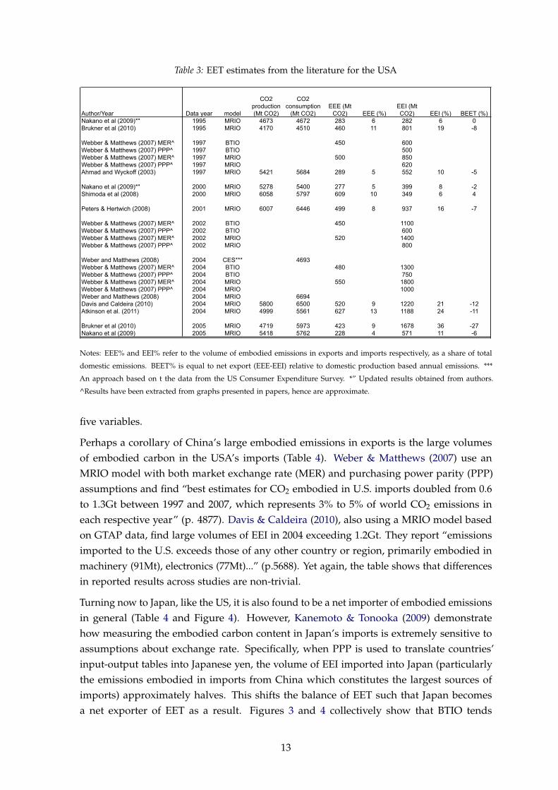
Table 3: EET estimates from the literature for the USA



CO2 consumption

(Mt CO2)EEE (Mt


Nakano et al (2009)*" 1995 MRIO 4673 4672 283 6 282 6 0Brukner et al (2010) 1995 MRIO 4170 4510 460 11 801 19 -8

Webber & Matthews (2007) MER^ 1997 BTIO 450 600Webber & Matthews (2007) PPP^ 1997 BTIO 500Webber & Matthews (2007) MER^ 1997 MRIO 500 850Webber & Matthews (2007) PPP^ 1997 MRIO 620Ahmad and Wyckoff (2003) 1997 MRIO 5421 5684 289 5 552 10 -5

Nakano et al (2009)*" 2000 MRIO 5278 5400 277 5 399 8 -2Shimoda et al (2008) 2000 MRIO 6058 5797 609 10 349 6 4

Peters & Hertwich (2008) 2001 MRIO 6007 6446 499 8 937 16 -7

Webber & Matthews (2007) MER^ 2002 BTIO 450 1100Webber & Matthews (2007) PPP^ 2002 BTIO 600Webber & Matthews (2007) MER^ 2002 MRIO 520 1400Webber & Matthews (2007) PPP^ 2002 MRIO 800

Weber and Matthews (2008) 2004 CES*** 4693Webber & Matthews (2007) MER^ 2004 BTIO 480 1300Webber & Matthews (2007) PPP^ 2004 BTIO 750Webber & Matthews (2007) MER^ 2004 MRIO 550 1800Webber & Matthews (2007) PPP^ 2004 MRIO 1000Weber and Matthews (2008) 2004 MRIO 6694Davis and Caldeira (2010) 2004 MRIO 5800 6500 520 9 1220 21 -12Atkinson et al. (2011) 2004 MRIO 4999 5561 627 13 1188 24 -11

Brukner et al (2010) 2005 MRIO 4719 5973 423 9 1678 36 -27Nakano et al (2009) 2005 MRIO 5418 5762 228 4 571 11 -6

Notes: EEE% and EEI% refer to the volume of embodied emissions in exports and imports respectively, as a share of total

domestic emissions. BEET% is equal to net export (EEE-EEI) relative to domestic production based annual emissions. ***

An approach based on t the data from the US Consumer Expenditure Survey. *” Updated results obtained from authors.

^Results have been extracted from graphs presented in papers, hence are approximate.

five variables.

Perhaps a corollary of China’s large embodied emissions in exports is the large volumesof embodied carbon in the USA’s imports (Table 4). Weber & Matthews (2007) use anMRIO model with both market exchange rate (MER) and purchasing power parity (PPP)assumptions and find “best estimates for CO2 embodied in U.S. imports doubled from 0.6to 1.3Gt between 1997 and 2007, which represents 3% to 5% of world CO2 emissions ineach respective year” (p. 4877). Davis & Caldeira (2010), also using a MRIO model basedon GTAP data, find large volumes of EEI in 2004 exceeding 1.2Gt. They report “emissionsimported to the U.S. exceeds those of any other country or region, primarily embodied inmachinery (91Mt), electronics (77Mt)...” (p.5688). Yet again, the table shows that differencesin reported results across studies are non-trivial.

Turning now to Japan, like the US, it is also found to be a net importer of embodied emissionsin general (Table 4 and Figure 4). However, Kanemoto & Tonooka (2009) demonstratehow measuring the embodied carbon content in Japan’s imports is extremely sensitive toassumptions about exchange rate. Specifically, when PPP is used to translate countries’input-output tables into Japanese yen, the volume of EEI imported into Japan (particularlythe emissions embodied in imports from China which constitutes the largest sources ofimports) approximately halves. This shifts the balance of EET such that Japan becomesa net exporter of EET as a result. Figures 3 and 4 collectively show that BTIO tends

13

Table 4: EET estimates from the literature for Japan



CO2 consumption

(Mt CO2)EEE (Mt


Kanemoto&Tonooka(2009)MER 1995 BTIO 1258 1387 147 12 276 22 -10Kanemoto&Tonooka(2009)PPP 1995 BTIO 1258 1221 147 12 110 9 3Ahmad and Wyckoff (2003) 1995 MRIO 1100 1287 102 9 289 26 -17Nakano et al (2009)*" 1995 MRIO 1051 1220 59 6 229 22 -16Brukner et al (2010) 1995 MRIO 978 1409 107 11 537 55 -44

Kanemoto&Tonooka(2009)MER 2000 BTIO 1308 1423 188 14 303 23 -9Kanemoto&Tonooka(2009)PPP 2000 BTIO 1308 1251 188 14 131 10 4Nakano et al (2009)*" 2000 MRIO 1076 1214 69 6 207 19 -13Shimoda et al (2008) 2000 MRIO 1051 1134 132 13 214 41 -8Nansai et al (2008) 2000 MRIO 939 291

Peters & Hertwich (2008) 2001 MRIO 1291 1489 187 15 385 30 -15

Davis and Caldiera (2010) 2004 MRIO 1310 1600 185 14 420 32 -18Atkinson et al. (2011) 2004 MRIO 940 1200 185 20 468 50 -30

Kanemoto&Tonooka(2009)MER 2005 BTIO 1335 1450 288 22 403 30 -9Kanemoto&Tonooka(2009)PPP 2005 BTIO 1335 1249 288 22 202 15 6Nakano et al (2009)*" 2005 MRIO 1114 1232 114 10 232 21 -11Brukner et al (2010) 2005 MRIO 1070 1450 211 20 592 55 -36


domestic emissions. BEET% is equal to net export (EEE-EEI) relative to domestic production based annual emissions. *”

Updated results obtained from authors.

to over-estimate EEE and MRIO underestimates EEE, an expected effect of the systemboundary difference. However, in contrast to Figure 3, Figure 4 shows that different studiesusing MRIO models can report wide ranging results. Atkinson et al. (2011) and Davis &Caldeira (2010), for example, both use GTAP 7 data but the former study leads to markedlyconservative estimates. The authors attribute this divergence to several factors includingthe omission of government and household demand in their modelling, the lower shareof global emissions that their model reattributes as embodied carbon in trade, and thedifference in country carbon accounts data used.

Overall, the broad picture emerging from the comparison of the results reported in theset of papers studied show large and growing volumes of embodied carbon emissions inglobal trade. This picture underlines the deepening of the global economic integrationprocess since the Kyoto Protocol was adopted in the 1990s. In line with the empirical tradeliterature (e.g. Backer & Yamano, 2008), it portrays a pattern of increasing intermediategoods trade and spatial fragmentation in production and consumption. It shows that notableand growing volumes of embodied carbon traded to and from both new and old centres ofproduction and consumption. As summarised by Hertwich & Peters (2010): “high densityOECD countries had higher emissions embodied in imports than exports, while for materialsexporters like Russia, Canada, Australia, Finland, Norway and South Africa, the situationwas the reverse. Emerging economies specialising in manufacturing, like China and Indiaalso had higher emissions in embodied exports and in imports.” (p.16).

Yet the quantities of the embodied carbon flows at country level remain highly uncertain formost countries and years. Significant inconsistencies are found when comparing reportedresults across the studies surveyed as shown in this section. Why such a large range ofestimates are being produced is evident from a description of the quantification approaches

14

Figure 4: Comparison of EET estimates from the literature for Japan in 2004-2005

Kanemoto&Tonooka(2009) MER

Kanemoto&Tonooka(2009) PPP

Davis & Caldiera (2010)

Atkinson et al. (2011)

Nakano et al (2009)

Brukner et al (2010)

BTIO, 2005 data

MRIO, 2004 data

MRIO, 2005 data

-200Mt Avg +200Mt

=1184Mt

Production emissions

-200Mt Avg +200Mt

=1363Mt

Consumption emissions

-200Mt Avg +200Mt

=212Mt

EEE

-200Mt Avg +200Mt

=386Mt

EEI

-40% 0 +40%

BEET

15

used; in practice many simplifications are necessary to overcome data, methodological andcomputational constraints in estimating embodied carbon flows. The next section describesthese issues that undermine the robustness of existing quantification of embodied emissions.

4 Issues contributing to uncertainty in EET estimation

4.1 Generic sources of uncertainty

4.1.1 Reliability of primary data

Although the data intensive nature of EET quantification is frequently noted, the reliabilityof the underlying statistics is often overlooked.

Economic input-output data: The quality of the input-output data depends on both theunderlying supply-use tables (SUT),14 and the procedure used for the complying thesymmetric input–output table. Druckman et al. (2008) conducts a simple test on the impactof the IO table compilation procedure on the UK embodied carbon results for 1995, andfinds that there is a “carbon inconsistency” of around 13% between the two methods.15

The two main sources of harmonised IO tables used for environmental MRIO modelling areOECD16 and the Global Trade Analysis Project.17 Additional uncertainties are introducedduring the process of interlinking and harmonizing IO tables for MRIO modelling, whichrequires multiple assumptions and aggregation of sectors (Weber et al., 2008). One papercautions: “...the GTAP database has considerable uncertainty, but it is unknown howbig this uncertainty is.”(Reinvang & Peters, 2008, p.31). Directly using SUTs for MRIOmodelling has been the favoured approach by some researchers to increase transparencyand disaggregation (e.g. Tukker et al. (2009). see Section 2.4), but this involves additionalassumptions and uncertainty.

Trade data: International trade statistics suffer from quality issues, in part due to thevoluntary nature of reporting trade data. Mirror statistics between two countries often donot match in bilateral trade data, due in part to differences between ci f (cost insuranceand freight) valuation typically used to record imports, and f ob (free on board) valuationfor exports (Lenzen et al., 2004).18 Several procedures have been developed to reconcile

14On the quality of SUTs, Thage (2005, p.14) notes “the size of sampling and non-sampling errors associatedwith the primary data on which the SUT is based, and the fact that a considerable part of the data contentsof the SUT is usually obtained by grossing-up methods, extrapolations, estimates of a more or less subjectivenature and even model calculations, should be taken into account when choosing the compilation method forthe SIOT”.

15The consistency check here for the estimated IO table from SUT gives the percentage difference between theleft and right-hand sides of the relationship x = (I � A)�1y where x is output and y is final demand.

16Used byAhmad & Wyckoff (2003), Nakano et al. (2009),Bruckner et al. (2010), Aichele & Felbermayr (2010)and Giljum et al. (2008).

17Used by Kainuma et al. (2000), Rodrigues et al. (2011), Atkinson et al. (2011), Peters & Hertwich (2008) andWilting & Vringer (2009)

18Other differences in reporting practises such as as definition of sectors and products, minimum levels andtime periods, as well as the treatment of unallocated or confidential trade also lead to discrepancies (Guo et al.,2009).

16

non-matching mirror statistics, such as GTAP’s reliability index approach (Narayanan &Walmsley, 2008).19 The degree of uncertainty associated with such methods are unknownand unverified. Moreover, additional uncertainty is induced when allocating bilateral tradeinto importing/ exporting sectors under the MRIO, as will be discussed in Section 4.2.3.

Environmental and emissions data: For the estimation of embodied emissions, reliableemission intensity coefficients are difficult to obtain particularly at a detailed sector leveland for developing countries (Liu & Wang, 2009). Peters et al. (2007) questions the accuracyof Chinese emission intensity data, in particular highlighting the uncertainty around thedecline in energy intensity between 1996 and 2000 and whether this was real or due tounder-reporting of coal consumption (see Akimoto et al. (2006)). Problems with the GTAPCO2 emissions data have also been noted – the quality is poor and may vary 10% to 20% fromUNFCCC data at the national level and may be greater at the sector level (Reinvang & Peters,2008). Moving towards EIO-LCA hybrid models, in theory, allows for more disaggregationof sectors and the capturing of international technology differences. However in practice,the availability of LCA-based carbon intensity data poses serious restrictions (Liu & Wang,2009).

4.1.2 Data coverage and aggregation

Geographical coverage and aggregation: Spatial disaggregation has several advantages,including improved representation of trade patterns and technology differences betweencountries and regions. For example, Su & Ang (2010) estimate China’s embodied carbon inexports using three levels of spatial aggregation. The authors find that when aggregated atthe country level using national average carbon intensities, emissions from the central coastand east coast regions (with lower carbon intensity) are overestimated whilst those from thenortheast and northwest (with higher carbon intensity) are underestimated. The net effect isa drop in total CO2 embodied in China’s export as the number of regions increase.

Whilst a multi-regional model may serve better from the perspective of representing techno-logy differences, there are trade-offs to be made with other sources of uncertainty. Andrewet al. (2009) examines the trade-off between complexity and accuracy in MRIO and findsthat including only the most important trade partner in terms of emissions embodied inimports and aggregating the rest of the world can substantially reduce the data requirementand achieve a good approximation to more complex models.

Greenhouse gas and sector coverage leads to systematic differences in EET estimates, hencestudies should make these explicit to aid the interpretation of the results (Lenzen & Murray,2001). The majority of studies considers only CO2 emissions from fossil fuel combustionand the most important differences are due to the inclusion/ exclusion of process emissions(e.g. from the cement and chemicals sectors) and the service sectors. . Some studies considera much wider scope of emissions – Lenzen (1998) includes CH4 and N2O due to fossilfuel consumption in addition to CO2, as well as CH4 and C2F6 due to industrial processes,

19GTAP trade data is based on UN COMTRADE and complimented with Global Trade Information Services(GTIS).

17

solvent use, agriculture, land use change, forestry and waste and fugitive emissions fromfossil fuel extraction.The latter study finds that differences in GHG coverage bounds is themain explanatory factor for the difference between their own conclusion that Australia isa net exporter of embodied emissions, and that of Common & Salma (1992)’s which findAustralia to have a balanced trade.

Sector Aggregation: Whilst MRIO models overcome issues with geographical aggregation,there is a trade-off with sector aggregation. The sector resolution of the model tends tobecome more coarse under MRIO models because of the process of matching datasets. Thisusually requires taking a lower common denominator, of the various levels of disaggregationavailable – USA and Japan produce tables of about 500 sectors, but Brazil has only 19.Harmonised tables tend to have around 50 sectors.20

Aggregation is also carried out to make the running of models computationally moremanageable but can lead to errors in estimates (this is referred to as aggregation bias inthe input-output literature) because input-output tables implicitly assumes one industrytechnology and homogeneity of firms producing for the domestic and export markets (Weisz& Duchin, 2006; Liu & Wang, 2009). This issue is particularly important for sectors withdifferentiated products such as the “non-metallic minerals sector” which includes clinker,cement, as well as basic and specialised glass products. Aggregation error is also importantwhere the sector’s trade composition does not reflect the production composition, orwhere technology is differentiated between export-demand and domestic-demand orientedproduction. 21

For macro or country level analysis, Tukker et al. (2009) argue that at least 100-150 sectorsare necessary in order to avoid lumping together important sectors with different emissionintensities, whilst Su et al. (2010) find that around 40 sectors are sufficient to capture theoverall share of embodied emissions in a country’s total exports. The extent of disaggregationnecessary, is in fact contingent on the policy question at hand. For sector level analysis,the policy question at hand should also guide the level of disaggregation necessary, asthe problem of heterogeneity can continue down to the product level – Maurer & Degain(2012) notes that “even in the most finely disaggregated import and export data, there arelarge differences in unit values of exports and imports across countries reflecting qualitydifferences that cannot be eliminated by disaggregation” (p.17).

20GTAP has 57 sectors, OECD harmonised tables have 48 sectors, and the Asian database from IDE-JETROhas 76 sectors (maximum). The EU mandates submission every five years, of harmonised tables (60 productsand 60 industries), however, there are some key gaps in the data availability.

21Lenzen et al. (2004) examines Denmark’s EET using a 128 sector model or an aggregated 10 sector model.For the uni-directional trade scenario, the authors find that total emissions produced remains the same in theclosed framework but aggregation results in a different distribution of EET across sectors. For the multi-regionaltrade scenario, the CO2 embodied in domestic final demand increases, mainly because the CO2 intensity ofthe aggregated ‘electricity, gas and water’ sector increases. This is, however, offset by the decreases of the CO2intensity of manufactured goods.

18

4.1.3 Using monetary data

The majority of top-down EET quantification rely on monetary data, to approximate physicalflows of goods. This assumes proportionality between monetary and physical flows. Thisnecessitates multiple assumptions which induce additional layers of uncertainty in estimat-ing EET, particularly in sectors where product heterogeneity is important (Maurer & Degain,2012; Reinvang & Peters, 2008).22 Using basic prices avoids some of the issues, but only to alimited extent (Muradian et al., 2002; Ahmad & Wyckoff, 2003; Weber & Matthews, 2007).23

Quantitatively, the error associated with assuming proportionality between monetary andphysical trade flows has been found to be significant – up to 40% for Australian energy andgreenhouse gas multipliers (Lenzen, 1998).

In addition, the use of monetary data requires assumptions about exchange rates – usingmarket exchange rate (MER) or purchasing power parity (PPP). Studies have repeatedlyshown that the results of EET estimation are very sensitive to this assumption. As shown inTable 4, Kanemoto & Tonooka (2009) report that using PPP reduces the estimate of Japan’sEEI by a third, compared with the same scenario using MER, largely due to the impact of theassumption on EEI from China. Weber & Matthews (2007) finds that “For most developedcountries, the difference between MER and PPP is relatively small, reflecting similar pricelevels. However, the difference between MER and PPP can be much higher for developingcountries – a factor of about 2 for Mexico and 4 for China in 1997... [it is] likely that the truevalue of EEI falls somewhere between the values calculated using MER and PPP and thatthe mix varies by commodity, as each commodity’s output in each country includes a mixof exports and domestically consumed goods, and the exports are usually valued higher perunit than domestically consumed goods. However, in the absence of physical unit data forthousands of commodities, this uncertainty is difficult to reduce.” (p. 4879).24

To overcome problems with monetary data, several studies integrate physical units intothe monetary core model (e.g. Machado et al., 2001; De Haan, 2001; Giljum, 2005; Weisz& Duchin, 2006; Giljum et al., 2010). Overall, the large sensitivity of EET estimates toassumptions used on price data suggests that studies that rely on monetary data should atminimum, test the sensitivity of results to the exchange rate assumption made.

22Even in the case where products are identical in a physical sense, they are often different in an economicsense in that they may be sold at different prices to different purchasers due to the existence of market power orlong term price contracts, as well as differences in the way transportation costs are invoiced, or in the way taxesor subsidies on production are accounted for.

23Basic prices tend to be more stable over time. The difference between basic prices and trade data in f.o.b.(free-on-board) and c.i.f. (cost-insurance-freight) is that includes tax. In Lenzen et al. (2004), economy-widebasic price-/f.o.b./c.i.f. ratios in order to convert imports into basic prices. Using physical quantities wouldavoid uncertainties induced by this conversion.

24Additionally, Hayami & Nakamura (2007) note that using monetary units and the industry-technologyassumption means that the aggregation error is never really eliminated, even if you have a high-resolutiondisaggregation of sectors. This is because almost always, firms produce multiple products, but the commonoverhead costs get spread across the different output products.

19

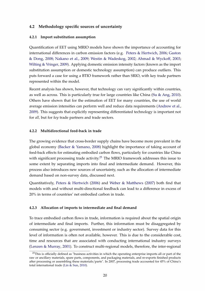
4.2 Methodology specific sources of uncertainty

4.2.1 Import substitution assumption

Quantification of EET using MRIO models have shown the importance of accounting forinternational differences in carbon emission factors (e.g. Peters & Hertwich, 2006; Gaston& Dong, 2008; Nakano et al., 2009; Westin & Wadeskog, 2002; Ahmad & Wyckoff, 2003;Wilting & Vringer, 2009). Applying domestic emission intensity factors (known as the importsubstitution assumption or domestic technology assumption) can produce outliers. Thisputs forward a case for using a BTIO framework rather than SRIO, with key trade partnersrepresented within the model.

Recent analysis has shown, however, that technology can vary significantly within countries,as well as across. This is particularly true for large countries like China (Su & Ang, 2010).Others have shown that for the estimation of EET for many countries, the use of worldaverage emission intensities can perform well and reduce data requirements (Andrew et al.,2009). This suggests that explicitly representing differentiated technology is important notfor all, but for key trade partners and trade sectors.

4.2.2 Multidirectional feed-back in trade

The growing evidence that cross-border supply chains have become more prevalent in theglobal economy (Backer & Yamano, 2008) highlight the importance of taking account offeed-back effects for estimating embodied carbon flows, particularly for countries like Chinawith significant processing trade activity.25 The MRIO framework addresses this issue tosome extent by separating imports into final and intermediate demand. However, thisprocess also introduces new sources of uncertainty, such as the allocation of intermediatedemand based on non-survey data, discussed next.

Quantitatively, Peters & Hertwich (2006) and Weber & Matthews (2007) both find thatmodels with and without multi-directional feedback can lead to a difference in excess of20% in terms of countries’ net embodied carbon in trade.

4.2.3 Allocation of imports to intermediate and final demand

To trace embodied carbon flows in trade, information is required about the spatial originof intermediate and final imports. Further, this information must be disaggregated byconsuming sector (e.g. government, investment or industry sector). Survey data for thislevel of information is often not available, however. This is due to the considerable cost,time and resources that are associated with conducting international industry surveys(Lenzen & Murray, 2001). To construct multi-regional models, therefore, the inter-regional

25This is officially defined as "business activities in which the operating enterprise imports all or part of theraw or ancillary materials, spare parts, components, and packaging materials, and re-exports finished productsafter processing or assembling these materials/parts". In 2007, processing trade accounted for 45% of China’stotal international trade (Lin & Sun, 2010).

20

Table 5: The characteristics of existing EET quantification approaches

System Boundary

Model typeTrade * intensity

(Physical)Trade * intensity

(Monetary) SRIO BTIO/EEBT MRIOHybrid MRIO-

LCATransparency Medium Medium High High Low LowAbility to capture time dimension High High Medium Medium Low LowLevel of sector disaggregation High Medium Medium Medium Low High

Capturesbilateral trade-partner info. n n n y

y (non-survey data)

y (non-survey data)

Captures differences in carbon intensities by country n n n y y y

domestic n n y y y y

international n n n n y yerror due to SUT conversion to IO n/a n/a Medium Medium High High

IO Harmonisation (e.g. different yearbase) n/a n/a n n High Highgeneric trade data issues Medium Medium Medium Medium High HighNon-survey estimation of origin of sector's imports n/a n/a n/a n/a y yaggregation error (sectors) n/a n/a Low Low High Medium

error due to lack of representation of technology differences High High High Low Low Mediumerror due to lack of feed-back loops High High High High Low Lowst

ruct

ural

Total demand Final Demand

Inte

r-se

ctor

al

trad

ere

gion

al

brea

kdow

n

Mod

el c

onst

ruct

ion

Dat

a is

sues

Vuln

erab

ility

to

sour

ce o

f un

cert

aint

y

Source: Author

intermediate trade component26 must be estimated, based on known variables and analyticalassumptions.

The standard non-survey approach used to estimate this is the trade share method, whichuses a region’s share in total global exports, and applies to all entries along the row ofthe imports matrix, for all using domestic industries and imported final demand vectors(Lenzen et al., 2004; Peters & Hertwich, 2006; Rodrigues et al., 2011).27Other methods areused by Rodrigues et al. (2011, p.52) which uses three additional estimation approaches28

and the project EXIOPOL which uses an alternative non-survey approach which is based onOosterhaven et al. (2008), as described in Tukker et al. (2009). The extent of adjustment inthe bilateral trade data to match the estimated intermediate trade component is unknown,however.

21

4.3 Summary

The data intensive exercise of estimating embodied carbon in trade involves multiplemethodological and data issues. Researchers in this field are faced with many trade-offs, forexample between regional and sectoral detail, or between policy relevance, cost, complexityand ease of estimation as well as robustness of the results (Table 5 summarises these trade-offs). Whilst some papers test the sensitivity of EET estimates to assumptions made intheir analysis, it can be said that the literature as a whole has so far paid little attention toensuring the measurement is sufficiently robust.

Moreover, clear statements of system boundaries, underlying assumptions and methodologyare noticeably absent in the literature (?Wiedmann & Minx, 2008). The large variations inthe estimates of country level embodied carbon in trade remains prevalent. As an increasingnumber of governments endorse the potential role of flow based indicators for environmentalpolicy evaluation and decision making, it is hoped that more structured analysis of thetrade-offs, as well as the suitability of different methods and system boundaries for theevaluation of different policy issues will emerge.

Assessing the accuracy of the reported volumes of EET is difficult because the results are notalways directly comparable to available survey data (the BTIO model is more comparable tonational trade balances whereas MRIO models are not (Peters, 2008b)). Nonetheless, theevaluation of the different sources of uncertainty in this section suggest some minimumrequirements for EET quantification analysis. For example, to address the fact that EETestimations are very sensitive to the assumption about technology, at minimum, the keytrading partners’ technologies should be accounted for. The import substitution assumptioncan lead to extreme results, hence there is a strong case for using BTIO over SRIO. Similarly,for country level estimations, it appears important to capture an appropriate amount ofsector detail, such that the important trading sectors are represented. It is not clear what theoptimum aggregation level is, but the literature suggests that good representation of thekey trading partners and sectors is more important than disaggregation and detail per se.The appropriate level of sector disaggregation will also depend on the motivating policyquestion.

In terms of system boundary, for countries with a high share of processing trade, thedistinction between using total and final demand is important. For such countries, itis important even in those cases where the model structure does not allow the explicitrepresentation of the multi-directional feed-back in trade (i.e. the MRIO framework is notused), that efforts is made to address the existence of high levels of re-exports. Huimin &Ye (2010), for example, apply a simple method in their study of China’s embodied carbon,using the share of processing trade and applying this to embodied emissions.

26This is usually represented by �Ars , or the inverse of matrix A of intermediate consumption of importedproducts from region s to region r to s.

27Using the notation from the latter, this is specified as tabij = im⇤b

ijexa⇤

⇤⇤ex⇤⇤

⇤⇤where tab

ij describes the flow from sectori in region a to sector j in region b, ⇤ denotes the sum of all values and imp and exp denote imports and exportsrespectively.

28These are: tabij = imp⇤b

ijexab

i⇤ex⇤b

i⇤; tab

ij = exabi⇤

imabij

im⇤bi⇤

; and tabij = exab

i⇤im⇤⇤

⇤jim⇤⇤

⇤⇤.

22

Although some of the issues associated with using monetary data are difficult to overcome,one that can and should be addressed is the assumption made when applying currencyexchange rates – using MER or PPP. This assumption in particular has been proven re-peatedly to strongly affect EET estimation levels. Sensitivity analysis should be conductedat minimum, to make a case for robustness of the results.

5 What does this mean for policy?

Embodied carbon in trade has been a subject of substantial interest in the academic andpolitical spheres. Estimates of EET flows can inform many policy questions, which canbe grouped into two broad levels. At a higher level, empirical understanding of embodiedcarbon in trade can help shape thinking around issues such as fairness in the allocationof responsibility between producers and consumers. At a lower level, more specific policyelements can be evaluated using EET estimates, for example, discussions around the carbonleakage concerns as well a measures to address such concerns. This section summarises thepolicy contexts in which embodied carbon have been measured, focusing on the higher level.It also evaluates the extent to which the existing literature can assist these debates, in lightof the degree of uncertainty involved in the quantification as highlighted in this paper thusfar.

5.1 Insights for higher level policy elements

Embodied carbon in trade has informed discussions around the fair allocation of respons-ibility between the producers and the consumers of emissions that are emitted throughoutthe multi-country processes linked by trade. There are a variety of views about the notionof fairness from a theoretical perspective. On the one extreme, some authors advocate thefull attribution of responsibility to the consumer. Other authors are in favour of sharedresponsibility principles, recognising that there are benefits accrued to both producers (e.g.value-added, jobs) and consumers (e.g. utility) along the chain (e.g. Kondo et al., 1998;Bastianoni et al., 2004; Ferng, 2003; Huimin & Ye, 2010). Lenzen et al. (2007) for examplepropose an allocation to each segment of the supply chain, depending on the share ofvalue-added. Rodrigues et al. (2011) also proposes a method to distribute responsibilityalong the chain, suggesting an even spread.29

Relatedly, the empirical literature on EET has evaluated the validity, efficacy and fairnessof using the production based approach to emissions accounting particularly as a basisfor international burden sharing agreements such as those under the Kyoto Protocol. Forexample, Druckman et al. (2008) quantify the volume of embodied emissions in UK’s importsand exports and concludes “any progress towards the UK’s carbon reduction targets (visible

29They define for each country or stage k, the total downstream embodied emissions EDk and a symmetrical

EUk which is the total upstream embodied emissions. They define total carbon responsibility of a country k as

Ek= aEUk + (1 � a)ED

k , suggesting a value of a half for a, hence an even distribution of responsibility betweenthe up and down streams.

23

under a production perspective) disappears completely when viewed from a consumptionperspective” (p. 594). Peters & Hertwich (2008) using a global MRIO model find that “from1996 to 2006 global CO2 emissions have increased by 35% even though Annex I countriesare still on target for a 5% reduction in 1990 GHG emissions by 2008-2012.” (p.1406). Thelatter paper also evaluates how the embodied carbon balances of countries may affecttheir incentives to participate in international agreements on climate change. They arguethat barriers to participation (as well as problems of carbon leakage) may be overcome byencouraging international coalition formation in defining emissions mitigation objectives.However, it is unclear what incentives are necessary to induce countries into such coalitionbuilding.

The assessment of sustainable development is another central motivation behind quan-tifying embodied emissions in trade at a higher level (e.g. Lenzen & Murray, 2001; Honget al., 2007). Resource flow based indicators for the global impacts of production andconsumption activities are officially endorsed by the European Union and OECD to sup-port environmental-economic decision making and to improve material flow and resourceproductivity, for example under EU’s Sustainable Development Strategy (European Commis-sion, 2004) and the EU Action Plan on Sustainable Consumption and Production (EuropeanCommission, 2008).30 Studies quantifying EET has also helped shape thinking around theimpact of trade on natural resource dependency and supply chain security. For example,Giljum et al. (2008) quantifies the embodied resource content of trade from a North-Southperspective and finds “trade pattern of net imports to the North is particularly visible forthe EU25, which faces the strongest dependence on resource imports of all investigatedworld regions, in particular regarding fossil fuels and metal ores.”(p.18). Machado et al.(2001) use estimates of Brazil’s embodied carbon and energy to highlight the adverse impactof trade promotion policies on export dependency and energy security.

To help address these higher level issues, suggestions have been made for presenting theconsumption based indicator alongside the usual territorial accounts to the UNFCCC (e.g.Wiedmann et al., 2011). Interestingly, the international agreement on HFC gases – MontrealProtocol – explicitly incorporates a consumption based perspective in the allocation ofmitigation responsibility (Ahmad & Wyckoff, 2003). In the case of carbon, however, themethodological and data considerations discussed in Section 4 limit the practical applicationof consumption based accounting in climate policy in a serious way. Indeed attempts inpublic policy to deviate away from the conventional production based carbon accountingapproach to account for EET has been met with hard opposition. For example, the Canadian“clean energy exports credit” proposal to the Kyoto Protocol was rejected (Zhang, 2004),as was Denmark’s plea to the European Union to deduct from their national accounts, theemissions for electricity which was consumed by Norwegian consumers (Lenzen et al.,2004). Nonetheless, these studies put forward a strong case for incorporating consumption

30Carbon footprint indicators extend from previous literature on ecological footprinting including carryingcapacity, bioproductivity and land disturbance. The ecological footprint was developed as an intuitively simple andelegant method for comparing the amount of productive land required to support the consumption of a givenpopulation indefinitely (Wackernagel et al., 1993). To measure the sustainability of a given population, this landarea is compared with the actual available land area.

24

based principles (for example as a shadow indicator) into strategies for CO2 mitigation, forexample to evaluate the drivers of global emissions or assess the environmental impactsconnected to national consumption (e.g. Peters & Solli, 2010).

5.2 Insights for lower level, detailed policy elements

At a lower level, the literature quantifying EET makes contributions towards more specificpolicy issues, in particular, the discourse on carbon leakage. Peters (2008a) suggests thedistinction between “strong” and “weak” carbon leakage. The former, narrower definitionconsiders only the geographical shift in production (and its associated emissions) in directresponse to climate policy, whilst ’weak’ carbon leakage extends the term to cover alltrade embodied emissions, whether the changes in trade level are driven by policy orby underlying economic factors e.g. international differences in labour price, industrialcapacity, technology, environmental standards and demand. It is argued the latter definitionis more conducive to discussing possible fruitful synergies between climate change andtrade policies (Peters & Hertwich, 2008; Peters, 2008a).

As an extension to the carbon leakage debate, quantifying EET has also enabled theevaluation of policies to regulate cross-border embodied emissions, such as border carbonmeasures.31 For example, by quantifying existing EET volumes and modelling differentmitigation and carbon price scenarios, Mattoo et al. (2009) assess the carbon leakage andwelfare effect of a border tax adjustment and find potential for large international transfersdue to such trade measures – in the direction from exporting to consuming countries. Thissuggests that countries with export industries may benefit from collecting a carbon taxdomestically and redistributing the revenue internally. By highlighting the difficulty ofmeasuring embodied carbon, the literature (e.g. Wiedmann et al., 2011) also suggests thatborder measures may in practice have to be based on averaged, rather than the actual carboncontent of traded goods, which in turn is likely to impact incentives for importers andexporters (Monjon & Quirion, 2011).

EET quantification has also led authors to advocate a sectoral perspective to approachingemissions mitigation. Weber et al. (2008, p.3577) and Carbon Trust (2011b) identify the inef-ficient and coal dominated electricity production in China as the main source of embodiedcarbon in consumption around the world. These authors suggest that policies promotingtechnology transfer in these carbon intensive industries may be more direct and effectivethan efforts to reduce trade (e.g. with a border carbon tax), partly because of the largeindirect role of the same industries in supplying each other, and also because of the potentialmagnitude of problems involved in agreeing a trade treaty.

Embodied carbon quantification has been shown to be a useful tool from the perspectiveof identifying carbon hotspots in a global supply chain (e.g. Carbon Trust, 2011a,b,c,e;Steinberger et al., 2009). Hayami & Nakamura (2007) using a case study on PV cellproduction in Japan and Canada finds that while it is desirable for countries to clean up

31Some of the recent debates can be found in Lockwood & Whalley (2008, 2010)

25

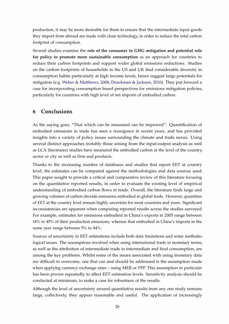
production, it may be more desirable for them to ensure that the intermediate input goodsthey import from abroad are made with clean technology, in order to reduce the total carbonfootprint of consumption.

Several studies examine the role of the consumer in GHG mitigation and potential rolefor policy to promote more sustainable consumption as an approach for countries toreduce their carbon footprints and support wider global emissions reductions. Studieson the carbon footprints of households in the US and UK find considerable diversity inconsumption habits particularly at high income levels, hence suggest large potentials formitigation (e.g. Weber & Matthews, 2008; Druckman & Jackson, 2010). They put forward acase for incorporating consumption based perspectives for emissions mitigation policies,particularly for countries with high level of net imports of embodied carbon.

6 Conclusions

As the saying goes, “That which can be measured can be improved”. Quantification ofembodied emissions in trade has seen a resurgence in recent years, and has providedinsights into a variety of policy issues surrounding the climate and trade nexus. Usingseveral distinct approaches (notably those arising from the input-output analysis as wellas LCA literatures) studies have measured the embodied carbon at the level of the country,sector or city as well as firm and products.

Thanks to the increasing number of databases and studies that report EET at countrylevel, the estimates can be compared against the methodologies and data sources used.This paper sought to provide a critical and comparative review of this literature focusingon the quantitative reported results, in order to evaluate the existing level of empiricalunderstanding of embodied carbon flows in trade. Overall, the literature finds large andgrowing volumes of carbon dioxide emissions embodied in global trade. However, quantitiesof EET at the country level remain highly uncertain for most countries and years. Significantinconsistencies are apparent when comparing reported results across the studies surveyed.For example, estimates for emissions embodied in China’s exports in 2005 range between18% to 45% of their production emissions, whereas that embodied in China’s imports in thesame year range between 5% to 44%.

Sources of uncertainty in EET estimations include both data limitations and some methodo-logical issues. The assumptions involved when using international trade in monetary terms,as well as the attribution of intermediate trade to intermediate and final consumption, areamong the key problems. Whilst some of the issues associated with using monetary dataare difficult to overcome, one that can and should be addressed is the assumption madewhen applying currency exchange rates – using MER or PPP. This assumption in particularhas been proven repeatedly to affect EET estimation levels. Sensitivity analysis should beconducted at minimum, to make a case for robustness of the results.

Although the level of uncertainty around quantitative results from any one study remainslarge, collectively, they appear reasonable and useful. The application of increasingly

26

sophisticated modelling techniques (particularly in MRIO modelling), discussions aroundthe creation of a meta-database for MRIO data32 as well as ongoing efforts to fill the datagaps reflect a significant level of interest invested in the potential for embodied carbonmeasurement for political and corporate decision making.

In fact, embodied carbon in trade arises in a variety of policy discourse surroundingclimate and trade, which can be grouped broadly into two levels. At a higher-level of policydiscussions, EET quantified at the country level has been used as a tool to deliberate issuesaround the fair allocation of mitigation responsibility in the presence of trade, as well asthe validity, efficacy and fairness of climate change policies founded on the conventionalproduction based emissions accounting and inventory. Explicitly incorporating consumptionbased principles can, in theory, improve fairness of outcomes in terms of the distributionof responsibility across producers and consumers. These principles have ben previouslyapplied in the context of global environmental agreements on HFC gases. Yet, this paperargued that in the case of carbon, the methodological and data considerations limit thepractical application of consumption based accounting in climate policy in a serious way.However, there may be a case for incorporating consumption based principles, for exampleas a shadow indicator, into strategies for CO2 mitigation for certain countries with large netimports of embodied carbon.

At a lower-level, EET flows quantified at the sector level have facilitated in discussions aroundthe carbon leakage concerns that surrounds the implementation of unilateral climate changepolicies. Although a review of the sector, firm or product level quantification of EET wasbeyond the scope of this paper, their potential policy implications were discussed. It wasfound that the empirical understanding of embodied carbon at the sector or supply chainlevel can provide useful insights for the potential design, functioning and distributionalconsequences of measures to address these concerns. It also opens new questions withregards to the role of trade in decarbonising these global supply chains, and the designof climate-trade integrated policies to support this. EET quantification at the productlevel suggest that policies promoting sustainable consumption can complement existingapproaches to drive down emissions in a production (through to consumption) chain.

Scope remains for further research at many levels – methodological, and empirical – in thequantification of embodied carbon. Sector level analysis seem especially timely for futureinvestigation.

References

Ahmad, N. & Wyckoff, A. (2003). Carbon dioxide tmissions tmbodied in internationaltrade of goods. OECD Science, Technology and Industry Working Papers 2003/15, OECDPublishing. 16, 19, 20, 24

32e.g. the OPEN EU project (http://www.oneplaneteconomynetwork.org) and the Reunion Project (Wiedmannet al., 2011).

27

Aichele, R. & Felbermayr, G. (2010). Kyoto and the carbon content of trade. FZID DiscussionPapers 10-2010, University of Hohenheim, Center for Research on Innovation and Services(FZID). Available from: https://fzid.uni-hohenheim.de/fileadmin/einrichtungen/

fzid/fzid_dp_2010_10_Felbermayr.pdf. 2, 9, 16

Akimoto, H., Ohara, T., Kurokawa, J., & Horii, N. (2006). Verification of energy consumptionin China during 1996-2003 by using satellite observational data. Atmospheric Environment,40, 7663–7667. 17

Andrew, R., Peters, G. P., & Lennox, J. (2009). Approximation and regional aggregation inmulti-regional input-output analysis for national carbon footprint accounting. EconomicSystems Research, 21(3), 311–335. 17, 20

Atkinson, G., Hamilton, K., Ruta, G., & Van Der Mensbrugghe, D. (2011). Trade in ‘virtualcarbon’: Empirical results and implications for policy. Global Environmental Change, 21(2),563–574. 14, 16

Ayres, R. U. & Kneese, A. V. (1969). Production, consumption, and externalities. TheAmerican Economic Review, 59(3), 282–297. 4

Backer, K. D. & Yamano, N. (2008). The measurement of globalisation using internationalinput-output tables. In OECD (Ed.), Staying competitive in the global economy: compendiumof studies on global value chains chapter 2, (pp. 37–64). Paris: OECD. Available from:http://browse.oecdbookshop.org/oecd/pdfs/product/9208061e.pdf#page=39. 14, 20

Bastianoni, S., Pulselli, F. M., & Tiezzi, E. (2004). The problem of assigning responsibility forgreenhouse gas emissions. Ecological Economics, 49(3), 253–257. 3, 23

Bruckner, M., Giljum, S., Lutz, C., & Wiebe, K. (2010). Consumption-based CO2 emissionsand carbon leakage: Results from the Global Resource Accounting Model GRAM. In Inter-national Conference on Economic Modeling (Ecomod 2010) Istanbul. Available from: http://ecomod.net/sites/default/files/document-conference/ecomod2010/1319.pdf. 8, 11,16

Carbon Trust (2011a). International carbon flows: Aluminium. CTC 790, Car-bon Trust, London. Available from: http://www.carbontrust.com/media/38366/

ctc790-international-carbon-flows_-aluminium.pdf. 25

Carbon Trust (2011b). International carbon flows: Automotive. CTC 792, Car-bon Trust, London. Available from: http://www.carbontrust.com/media/38401/

ctc792-international-carbon-flows-automotive.pdf. 25

Carbon Trust (2011c). International carbon flows: Cotton. CTC 794, Car-bon Trust, London. Available from: http://www.carbontrust.com/media/38354/

ctc794-international-carbon-flows-cotton.pdf. 25

Carbon Trust (2011d). International carbon flows: Global flows. CTC 795, Car-bon Trust, London. Available from: http://www.carbontrust.com/media/38075/

ctc795-international-carbon-flows-global-flows.pdf. 2

28

https://fzid.uni-hohenheim.de/fileadmin/einrichtungen/fzid/fzid_dp_2010_10_Felbermayr.pdf

https://fzid.uni-hohenheim.de/fileadmin/einrichtungen/fzid/fzid_dp_2010_10_Felbermayr.pdf

http://browse.oecdbookshop.org/oecd/pdfs/product/9208061e.pdf#page=39

http://ecomod.net/sites/default/files/document-conference/ecomod2010/1319.pdf

http://ecomod.net/sites/default/files/document-conference/ecomod2010/1319.pdf

http://www.carbontrust.com/media/38366/ctc790-international-carbon-flows_-aluminium.pdf

http://www.carbontrust.com/media/38366/ctc790-international-carbon-flows_-aluminium.pdf

http://www.carbontrust.com/media/38401/ctc792-international-carbon-flows-automotive.pdf

http://www.carbontrust.com/media/38401/ctc792-international-carbon-flows-automotive.pdf

http://www.carbontrust.com/media/38354/ctc794-international-carbon-flows-cotton.pdf

http://www.carbontrust.com/media/38354/ctc794-international-carbon-flows-cotton.pdf

http://www.carbontrust.com/media/38075/ctc795-international-carbon-flows-global-flows.pdf

http://www.carbontrust.com/media/38075/ctc795-international-carbon-flows-global-flows.pdf

Carbon Trust (2011e). International carbon flows: Steel. CTC 791, Car-bon Trust, London. Available from: http://www.carbontrust.com/media/38362/

ctc791-international-carbon-flows-steel.pdf. 25

Common, M. S. & Salma, U. (1992). Accounting for changes in Australian carbon dioxideemissions. Energy Economics, 14(3), 217–225. 18

Davis, S. J. & Caldeira, K. (2010). Consumption-based accounting of CO2 emissions. Proceed-ings of the National Academy of Sciences, 107(12), 5687–5692. 2, 9, 13, 14

Dawkins, E., Roelich, K., & Owen, A. (2010). A consumption approach foremissions accounting - The REAP tool and REAP data for 2006. SEI Pro-ject Report, Stockholm Environment Institute, Stockholm. Available from:http://www.sei-international.org/mediamanager/documents/Publications/

Rethinking-development/SEI_Report_REAP_Documentation_2010.pdf. 8

De Haan, M. (2001). A structural decomposition analysis of pollution in the Netherlands.Economic Systems Research, 13(2), 181–196. 19

Druckman, A., Bradley, P., Papathanasopoulou, E., & Jackson, T. (2008). Measuring progresstowards carbon reduction in the UK. Ecological Economics, 66(4), 594–604. 16, 23

Druckman, A. & Jackson, T. (2010). The bare necessities: How much household carbon dowe really need? Ecological Economics, 69(9), 1794–1804. 26

Ellermann, C., Oliver, P., & Xingyu, L. (2009). Competitiveness and carbon leakage: Im-plications for China and the world. In Conference on the International Dimensions of Cli-mate Policies Bern. Available from: http://www.nccr-climate.unibe.ch/conferences/

climate_policies/working_papers/Ellermann.pdf. 10

European Commission (2004). Communication from the Commission to the Counciland the European Parliament - Stimulating technologies for sustainable development:An environmental technologies action plan for the European Union. Communica-tion COM/2004/0038 final, European Commission, Brussels. Available from: http:

//eur-lex.europa.eu/LexUriServ/LexUriServ.do?uri=CELEX:52004DC0038:EN:NOT. 24

European Commission (2008). Communication from the Commission to the EuropeanParliament, the Council, the European Economic and Social Committee and the Committeeof the Regions on the sustainable consumption and production and sustainable industrialpolicy action plan {SEC(2008) 2110} {SEC(2008) 2111}. Communication COM/2008/0397final, European Commission, Brussels. Available from: http://eur-lex.europa.eu/

LexUriServ/LexUriServ.do?uri=CELEX:52008DC0397:EN:NOT. 24

Ferng, J.-J. (2003). Allocating the responsibility of CO2 over-emissions from the perspectivesof benefit principle and ecological deficit. Ecological Economics, 46(1), 121–141. 23

Gaston, C. & Dong, L. (2008). CO2 emissions from Chinese imports. In International Input-Output Meeting on Managing the Environment Seville. Available from: http://www.iioa.org/pdf/Intermediate-2008/Papers/4a2_Gaston.pdf. 20

29

http://www.carbontrust.com/media/38362/ctc791-international-carbon-flows-steel.pdf

http://www.carbontrust.com/media/38362/ctc791-international-carbon-flows-steel.pdf

http://www.sei-international.org/mediamanager/documents/Publications/Rethinking-development/SEI_Report_REAP_Documentation_2010.pdf

http://www.sei-international.org/mediamanager/documents/Publications/Rethinking-development/SEI_Report_REAP_Documentation_2010.pdf

http://www.nccr-climate.unibe.ch/conferences/climate_policies/working_papers/Ellermann.pdf

http://www.nccr-climate.unibe.ch/conferences/climate_policies/working_papers/Ellermann.pdf

http://eur-lex.europa.eu/LexUriServ/LexUriServ.do?uri=CELEX:52004DC0038:EN:NOT




http://www.iioa.org/pdf/Intermediate-2008/Papers/4a2_Gaston.pdf

http://www.iioa.org/pdf/Intermediate-2008/Papers/4a2_Gaston.pdf

Giljum, S. (2005). Quantifying indirect natural resource requirements with a global mul-ticountry input-output model. In Proceedings of the conference “Environmental Accountingand Sustainable Development Indicators” (pp. 183–189). Prague: The Charles UniversityEnvironmental Center. 19

Giljum, S., Lutz, C., Jungnitz, A., Bruckner, M., & Hinterberger, F. (2008). Global dimensionsof European natural resource use: First results from the Global Resource AccountingModel (GRAM). SERI Working Paper 7, Sustainable Europe Research Institute, Vienna.Available from: http://seri.at/wp-content/uploads/2009/08/SERI-Working-Paper-7.pdf. 8, 16, 24

Giljum, S., Polzin, C., & Lutz, C. (2010). Global implications of a european environmental taxreform. SERI Working Paper 10, Sustainable Europe Research Institute, Vienna. Availablefrom: http://seri.at/wp-content/uploads/2010/02/SERI-Working-Paper-10.pdf. 8,19

Green Design Institute. Economic Input-Output Life Cycle Assessment (EIO-LCA) [online].(2009). Carnegie Mellon University. Available from: http://www.eiolca.net/. 6

Guo, D., Webb, C., & Yamano, N. (2009). Towards harmonised bilateral trade data forinter-country input-output analysis: Statistical issues. OECD Science, Technology andIndustry Working Papers 2009/4, OECD Publishing. 16

Hayami, H. & Nakamura, M. (2007). Greenhouse gas emissions in Canada and Japan: Sector-specific estimates and managerial and economic implications. Journal of EnvironmentalManagement, 85(2), 371–392. 19, 25

Helm, D., Smale, R., & Phillips, J. (2007). Too good to be true? The UK’s climate changerecord. [Online], Dieter Helm CBE. Available from: http://www.dieterhelm.co.uk/

sites/default/files/Carbon_record_2007.pdf. 7

Herendeen, R. A. (1978). Input-output techniques and energy cost of commodities. EnergyPolicy, 6(2), 162–165. 2

Hertwich, E. G. & Peters, G. P. (2009). Carbon footprint of nations: A global, trade-linkedanalysis. Environmental Science & Technology, 43(16), 6414–6420. 8

Hertwich, E. G. & Peters, G. P. (2010). Multiregional input-output database.OPEN: EU Technical Document, One Planet Economy Network. Availablefrom: http://www.oneplaneteconomynetwork.org/resources/programme-documents/

WP1_MRIO_Technical_Document.pdf. 3, 8, 14

Hoekstra, A. Y. & Hung, P. Q. (2005). Globalisation of water resources: International virtualwater flows in relation to crop trade. Global Environmental Change, 15(1), 45–56. 2

Hong, L., Dong, Z. P., Chunyu, H., & Gang, W. (2007). Evaluating the effects of embodiedenergy in international trade on ecological footprint in China. Ecological Economics, 62(1),136–148. 24

30

http://seri.at/wp-content/uploads/2009/08/SERI-Working-Paper-7.pdf



http://www.eiolca.net/

http://www.dieterhelm.co.uk/sites/default/files/Carbon_record_2007.pdf

http://www.dieterhelm.co.uk/sites/default/files/Carbon_record_2007.pdf

http://www.oneplaneteconomynetwork.org/resources/programme-documents/WP1_MRIO_Technical_Document.pdf

http://www.oneplaneteconomynetwork.org/resources/programme-documents/WP1_MRIO_Technical_Document.pdf

Huimin, L. & Ye, Q. (2010). Carbon embodied in international trade of China and itsemission responsibility. Chinese Journal of Population, Resources and Environment, 8(2), 24–31.10, 11, 22, 23

IEA (2008). World energy outlook 2008. Paris: International Energy Agency (OECD/IEA). 2, 9

IPCC (1996). Revised 1996 IPCC guidelines for national greenhouse gas inventories. Work-book (Volume 2), Intergovermental Panel on Climate Change, Geneva. Available from:http://www.ipcc-nggip.iges.or.jp/public/gl/invs5.html. 3

Kainuma, M., Matsuoka, Y., & Morita, T. (2000). Estimation of embodied CO2 emissions bygeneral equilibrium model. European Journal of Operational Research, 122(2), 392–404. 6, 16

Kanemoto, K., Lenzen, M., Geschke, A., & Moran, D. (2012). Building Eora:a global multi-region input-output model at high country and sector resolution.In Proceedings of The 20th International Input-Output Conference Bratislava. Avail-able from: http://www.iioa.org/files/conference-3/700_20120110120_LenzenEtAl_

BuildingEora_BratislavaIOConf.pdf. 8

Kanemoto, K. & Tonooka, Y. (2009). Embodied CO2 emissions in Japan’s international trade.Journal of Japan Society of Energy and Resources, 30(2), 15–23. 13, 19

Kondo, Y., Moriguchi, Y., & Shimizu, H. (1998). CO2 emissions in Japan: Influences ofimports and exports. Applied Energy, 59(2-3), 163–174. 23

Lenzen, M. (1998). Primary energy and greenhouse gases embodied in Australian finalconsumption: An input-output analysis. Energy Policy, 26(6), 495–506. 17, 19

Lenzen, M. (2001). Errors in conventional and input-output-based life-cycle inventories.Journal of Industrial Ecology, 4(4), 127–148. 6

Lenzen, M. (2011). Aggregation versus disaggregation in input–output analysis of theenvironment. Economic Systems Research, 23(1), 73–89. 8

Lenzen, M., Kanemoto, K., Geschke, A., Moran, D., Muñoz, P., Ugon, J., Wood, R., & Ting, Y.(2010a). A global multi-region input-output time series at high country and sector detail.In Proceedings for The 18th International Input Output Conference Sydney. 8

Lenzen, M., Murray, J., Sack, F., & Wiedmann, T. (2007). Shared producer and consumerresponsibility – Theory and practice. Ecological Economics, 61(1), 27–42. 3, 23

Lenzen, M. & Murray, S. A. (2001). A modified ecological footprint method and its applica-tion to Australia. Ecological Economics, 37(2), 229–255. 2, 17, 20, 24

Lenzen, M., Pade, L.-L., & Munksgaard, J. (2004). CO2 multipliers in multi-region input-output models. Economic Systems Research, 16(4), 391–412. 16, 18, 19, 21, 24

Lenzen, M., Wood, R., & Wiedmann, T. (2010b). Uncertainty analysis for multi-region input-output models – a case study of the UK’s carbon footprint. Economic Systems Research,22(1), 43–63. 8

31

http://www.ipcc-nggip.iges.or.jp/public/gl/invs5.html

http://www.iioa.org/files/conference-3/700_20120110120_LenzenEtAl_BuildingEora_BratislavaIOConf.pdf

http://www.iioa.org/files/conference-3/700_20120110120_LenzenEtAl_BuildingEora_BratislavaIOConf.pdf

Leontief, W. (1970). Environmental Repercussions and the Economic Structure: An Input-Output Approach. The Review of Economics and Statistics, 52(3), 262–271. 4

Lin, B. & Sun, C. (2010). Evaluating carbon dioxide emissions in international trade of China.Energy Policy, 38(1), 613–621. 11, 20

Liu, X. & Wang, C. (2009). Quantitative analysis of CO2 embodiment in international trade:An overview of emerging literatures. Frontiers of Environmental Science & Engineering inChina, 3(1), 12–19. 3, 6, 17, 18

Lockwood, B. & Whalley, J. (2008). Climate change-related border tax adjustments. CIGIPolicy Brief 4, The Centre for International Governance Innovation, Ontario. Availablefrom: http://dspace.cigilibrary.org/jspui/bitstream/123456789/24495/1/Policy_

Brief_no4.pdf?1. 25

Lockwood, B. & Whalley, J. (2010). Carbon-motivated border tax adjustments: Old wine ingreen bottles? World Economy, 33(6), 810–819. 25

Lutter, S., Giljum, S., Wilting, H., Widemann, T., & Palm, V. (2008). Interim-report on theresults of the evaluation of methodologies assessed with the RACER framework. EIPOTWork Package 3, Scientific Knowledge for Environmental Protection (SKEP) EnvironmentalImpact of Trade (EIPOT) Project. Available from: http://www.sei.se/eipot/resources/EIPOT-Interim-Report-final2007Oct08.pdf. 3, 8

Machado, G., Schaeffer, R., & Worrell, E. (2001). Energy and carbon embodied in theinternational trade of Brazil: An input-output approach. Ecological Economics, 39(3),409–424. 19, 24

Mattoo, A., Subramanian, A., van der Mensbrugghe, D., & He, J. (2009). Reconciling climatechange and trade policy. Working Paper WP 09-15, The Peterson Institute for InternationalEconomics, Washington, DC. Available from: http://www.piie.iie.com/publications/wp/wp09-15.pdf. 25

Maurer, A. & Degain, C. (2012). Globalization and trade flows: What you see is not whatyou get! Journal of International Commerce, Economics and Policy, 03(03), 1250019 1–27. 18, 19

Miller, R. E. & Blair, P. D. (1985). Input-output analysis: Foundations and extensions. EnglewoodCliffths, N.J.: Prentice-Hall. 4

Moll, S., Acosta, J., Giljum, S., Lutter, S., Pulles, M. T., & Kuenen, J. (2008). Creatinga global environmental database for input-output applications environmental exten-sions in the EXIOPOL project. In The Intermediate Input-Output Meeting on Managing theEnvironment Seville. Available from: http://old.seri.at/documentupload/SERI%20PR/Projekte/paper_iiomme_molletal.pdf. 8

Monjon, S. & Quirion, P. (2011). A border adjustment for the EU ETS: Reconciling WTOrules and capacity to tackle carbon leakage. Climate Policy, 11(5), 1212–1225. 25

32

http://dspace.cigilibrary.org/jspui/bitstream/123456789/24495/1/Policy_Brief_no4.pdf?1

http://dspace.cigilibrary.org/jspui/bitstream/123456789/24495/1/Policy_Brief_no4.pdf?1

http://www.sei.se/eipot/resources/EIPOT-Interim-Report-final2007Oct08.pdf

http://www.sei.se/eipot/resources/EIPOT-Interim-Report-final2007Oct08.pdf

http://www.piie.iie.com/publications/wp/wp09-15.pdf

http://www.piie.iie.com/publications/wp/wp09-15.pdf

http://old.seri.at/documentupload/SERI%20PR/Projekte/paper_iiomme_molletal.pdf

http://old.seri.at/documentupload/SERI%20PR/Projekte/paper_iiomme_molletal.pdf

Munksgaard, J. & Pedersen, K. A. (2001). CO2 accounts for open economies: producer orconsumer responsibility? Energy Policy, 29(4), 327–334. 3

Muradian, R., O’Connor, M., & Martinez-Alier, J. (2002). Embodied pollution in trade:Estimating the ‘environmental load displacement’ of industrialised countries. EcologicalEconomics, 41(1), 51–67. 19

Nakano, S., Okamura, A., Sakurai, N., Suzuki, M., Tojo, Y., & Yamano, N. (2009). Themeasurement of CO2 embodiments in international trade: Evidence from the harmonisedinput-output and bilateral trade database. OECD Science, Technology and IndustryWorking Papers 2009/03, OECD Publishing. Available from: http://dx.doi.org/10.

1787/227026518048. 11, 16, 20

Narayanan, G. B. & Walmsley, T. L. (2008). Global trade, assistance, and production: TheGTAP 7 data base. Center for Global Trade Analysis, Purdue University. Available from:https://www.gtap.agecon.purdue.edu/databases/v7/v7_doco.asp. 17

Oki, T. & Kanae, S. (2004). Virtual water trade and world water resources. Water Science &Technology, 49(7), 203–209. 2

Oosterhaven, J., Stelder, D., & Inomata, S. (2008). Estimating international interindustrylinkages: Non-survey simulations of the Asian-Pacific economy. Economic Systems Research,20(4), 395–414. 21

Pandey, D., Agrawal, M., & Pandey, J. S. (2010). Carbon footprint: current methods ofestimation. Environmental Monitoring and Assessment, 178, 135–160. Available from: http://www.springerlink.com.gate2.library.lse.ac.uk/content/g531t74mvh500125/. 4

Peters, G. (2008a). Reassessing carbon leakage. In The 11th Annual Conference on GlobalEconomic Analysis “Future of Global Economy” Helsinki. Available from: https://www.gtap.agecon.purdue.edu/resources/download/3751.pdf. 7, 25

Peters, G. & Hertwich, E. (2008). CO2 embodied in international trade with implications forglobal climate policy. Environmental Science & Technology, 42(5), 1401–1407. 2, 8, 16, 24, 25

Peters, G. & Solli, C. (2010). Global carbon footprints: Methods and import and export correctedresults from the Nordic countries in global carbon footprint studies. Copenhagen: Norden: TheNordic Council & Nordic Council of Ministers. 3, 4, 6, 8, 25

Peters, G. P. (2008b). From production-based to consumption-based national emissioninventories. Ecological Economics, 65(1), 13–23. 6, 22

Peters, G. P., Andrew, R., & Lennox, J. (2011a). Constructing an environmentally-extendedmulti-regional input-output table using the GTAP data. Economic Systems Research, 23(2),131–152. 8

Peters, G. P. & Hertwich, E. G. (2006). Pollution embodied in trade: The Norwegian case.Global Environmental Change, 16(4), 379–387. 20, 21

33

http://dx.doi.org/10.1787/227026518048

http://dx.doi.org/10.1787/227026518048

https://www.gtap.agecon.purdue.edu/databases/v7/v7_doco.asp

http://www.springerlink.com.gate2.library.lse.ac.uk/content/g531t74mvh500125/

http://www.springerlink.com.gate2.library.lse.ac.uk/content/g531t74mvh500125/

https://www.gtap.agecon.purdue.edu/resources/download/3751.pdf

https://www.gtap.agecon.purdue.edu/resources/download/3751.pdf

Peters, G. P., Minx, J. C., Weber, C. L., & Edenhofer, O. (2011b). Growth in emission transfersvia international trade from 1990 to 2008. Proceedings of the National Academy of Sciences,108(21), 8533–8534. 2, 8, 9

Peters, G. P., Weber, C. L., Guan, D., & Hubacek, K. (2007). China’s growing CO2 emissions– A race between increasing consumption and efficiency gains. Environmental Science &Technology, 41(17), 5939–5944. 7, 17

Proops, J. L. R. (1977). Input-output analysis and energy intensities: A comparison of somemethodologies. Applied Mathematical Modelling, 1(4), 181–186. 2

Reinvang, R. & Peters, G. (2008). Norwegian consumption, Chinese pollution. Technicalreport, WWF Norway, WWF China Programme Office, Norwegian University of Sci-ence and Technology. Available from: http://assets.wwf.no/downloads/wwfrapport_

jan2008_norsk_klimaavtrykk_i_kina_1.pdf. 16, 17, 19

Rodrigues, J. A., Domingos, T., Giljum, S., & Schneider, F. A. (2006). Designing an indicatorof environmental responsibility. Ecological Economics, 59(3), 256–266. 3

Rodrigues, J. F. D., Domingos, T. M. D., & Marques, A. P. (2011). Carbon responsibility andembodied emissions: Theory and measurement. Routledge, Taylor & Francis Group. 6, 16, 21,23

Shui, B. & Harriss, R. C. (2006). The role of CO2 embodiment in US-China trade. EnergyPolicy, 34(18), 4063–4068. 6

Steinberger, J. K., Friot, D., Jolliet, O., & Erkman, S. (2009). A spatially explicit life cycleinventory of the global textile chain. The International Journal of Life Cycle Assessment, 14,443–455. 25

Su, B. & Ang, B. W. (2010). Input-output analysis of CO2 emissions embodied in trade: Theeffects of spatial aggregation. Ecological Economics, 70(1), 10–18. 17, 20

Su, B., Huang, H. C., Ang, B. W., & Zhou, P. (2010). Input-output analysis of CO2 emissionsembodied in trade: The effects of sector aggregation. Energy Economics, 32(1), 166–175. 18

Subak, S. (1995). Methane embodied in the international trade of commodities : Implicationsfor global emissions. Global Environmental Change, 5(5), 433–446. 2

Thage, B. (2005). Symmetric input-output tables: Compilation issues. In 15th InternationalInput-Output Conference Beijin. Available from: http://www.iioa.org/pdf/15th%20Conf/thage.pdf. 16

Tukker, A., Poliakov, E., Heijungs, R., Hawkins, T., Neuwahl, F., Rueda-Cantuche, J. A. M.,Giljum, S., Moll, S., Oosterhaven, J., & Bouwmeester, M. (2009). Towards a global multi-regional environmentally extended input-output database. Ecological Economics, 68(7),1928–1937. 4, 8, 16, 18, 21

34

http://assets.wwf.no/downloads/wwfrapport_jan2008_norsk_klimaavtrykk_i_kina_1.pdf

http://assets.wwf.no/downloads/wwfrapport_jan2008_norsk_klimaavtrykk_i_kina_1.pdf

http://www.iioa.org/pdf/15th%20Conf/thage.pdf

http://www.iioa.org/pdf/15th%20Conf/thage.pdf

Wackernagel, M., McIntosh, J., Rees, W. E., & Woollard, R. (1993). How big is our ecologicalfootprint? A handbook for estimating a community’s appropriated carrying capacity. Vancouver:University of British Columbia. Discussion draft of the UBC Task Force on PlanningHealthy and Sustainable Communities. 24

Wang, T. & Watson, J. (2008). China’s carbon emissions and international trade: Implicationsfor post-2012 policy. Climate Policy, 8, 577–587. 6

Weber, C. L. (2008). Uncertainties in constructing environmental multiregional input-output models. In International Input-Output Meeting on Managing the Environment Seville.Available from: http://www.iioa.org/pdf/Intermediate-2008/Papers/5d4_Weber.pdf.3, 6

Weber, C. L. & Matthews, H. S. (2007). Embodied environmental emissions in U.S. interna-tional trade, 1997-2004. Environmental Science & Technology, 41(14), 4875–4881. 8, 13, 19,20

Weber, C. L. & Matthews, H. S. (2008). Quantifying the global and distributional aspects ofAmerican household carbon footprint. Ecological Economics, 66(2-3), 379–391. 8, 26

Weber, C. L. & Peters, G. P. (2009). Climate change policy and international trade: Policyconsiderations in the US. Energy Policy, 37(2), 432–440. 8

Weber, C. L., Peters, G. P., Guan, D., & Hubacek, K. (2008). The contribution of Chineseexports to climate change. Energy Policy, 36(9), 3572–3577. 11, 12, 16, 25

Weisz, H. & Duchin, F. (2006). Physical and monetary input-output analysis: What makesthe difference? Ecological Economics, 57(3), 534–541. 18, 19

Westin, J. & Wadeskog, A. (2002). The environmental impact of swedish trade. MI71Environmental accounts MI71ÖP0202, Statistiska centralbyrån (SCB) - Statistics Sweden.Available from: http://www.scb.se/statistik/MI/MI1202/2000I02/MI71OP0202.pdf. 20

Wichelns, D. (2001). The role of ‘virtual water’ in efforts to achieve food security andother national goals, with an example from Egypt. Agricultural Water Management, 49(2),131–151. 2

Wiedmann, T. (2009). A review of recent multi-region input-output models used forconsumption-based emission and resource accounting. Ecological Economics, 69(2), 211–222.5

Wiedmann, T. & Lenzen, M. (2007). On the conversion between local and global hectares inecological footprint analysis. Ecological Economics, 60(4), 673–677. 6

Wiedmann, T. & Minx, J. (2008). A definition of ‘carbon footprint’. In C. Pertsova (Ed.),Ecological economics research trends. Hauppauge NY: Nova Science Publishers. 22

Wiedmann, T., Wilting, H., Lutter, S., Palm, V., Giljum, S., Wadeskog, A., & Nijdam, D.(2009). Development of a methodology for the assessment of global environmental impacts

35

http://www.iioa.org/pdf/Intermediate-2008/Papers/5d4_Weber.pdf

http://www.scb.se/statistik/MI/MI1202/2000I02/MI71OP0202.pdf

of traded goods and services. Final report, Scientific Knowledge for EnvironmentalProtection (SKEP) Environmental Impact of Trade (EIPOT) Project. Available from:http://seri.at/wp-content/uploads/2010/06/development.pdf. 3, 4, 5, 8

Wiedmann, T., Wilting, H. C., Lenzen, M., Lutter, & Palm, V. (2011). Quo vadis MRIO?methodological, data and institutional requirements for multi-region input-output analysis.Ecological Economics, 70(11), 1937–1945. 3, 8, 24, 25, 27

Wiedmann, T., Wood, R., Lenzen, M., Minx, J., Guan, D., & Barrett, J. (2008). Developmentof an embedded carbon emissions indicator – producing a time series of input-outputtables and embedded carbon dioxide emissions for the UK by using a MRIO data op-timisation system. Report to the UK Department for Environment, Food and RuralAffairs, by the Stockholm Environment Institute and the University of Sydney, Defra,London. Available from: http://www.isa.org.usyd.edu.au/publications/documents/Defra_EmbeddedCarbon_Main.pdf. 7, 8, 11

Wiedmann, T., Wood, R., Minx, J. C., Lenzen, M., Guan, D., & Harris, R. (2010). A carbonfootprint time series of the UK – Results from a multi-regional input-output model.Economic Systems Research, 22(1), 19–42. 8

Wilting, H. C. & Vringer, K. (2009). Carbon and land use accounting from a producer’sand a consumer’s perspective – An empirical examination covering the world. EconomicSystems Research, 21(3), 291–310. 16, 20

Wood, R. & Lenzen, M. (2009). Structural path decomposition. Energy Economics, 31(3),335–341. 8

World Trade Organisation (2012). WTO Statistics Database. Available from: http://stat.wto.org/Home/WSDBHome.aspx?Language=E. 2

Yan, Y. & Yang, L. (2009). China’s foreign trade and climate change: A case study of CO2

emissions. Energy Policy, 38(1), 350–356. 3, 11

Zhang, Z. X. (2004). Open trade with the US without compromising Canada. Journal ofWorld Trade, 38(1), 155–182. 24

7 Appendix

36

http://seri.at/wp-content/uploads/2010/06/development.pdf

http://www.isa.org.usyd.edu.au/publications/documents/Defra_EmbeddedCarbon_Main.pdf

http://www.isa.org.usyd.edu.au/publications/documents/Defra_EmbeddedCarbon_Main.pdf

http://stat.wto.org/Home/WSDBHome.aspx?Language=E

http://stat.wto.org/Home/WSDBHome.aspx?Language=E

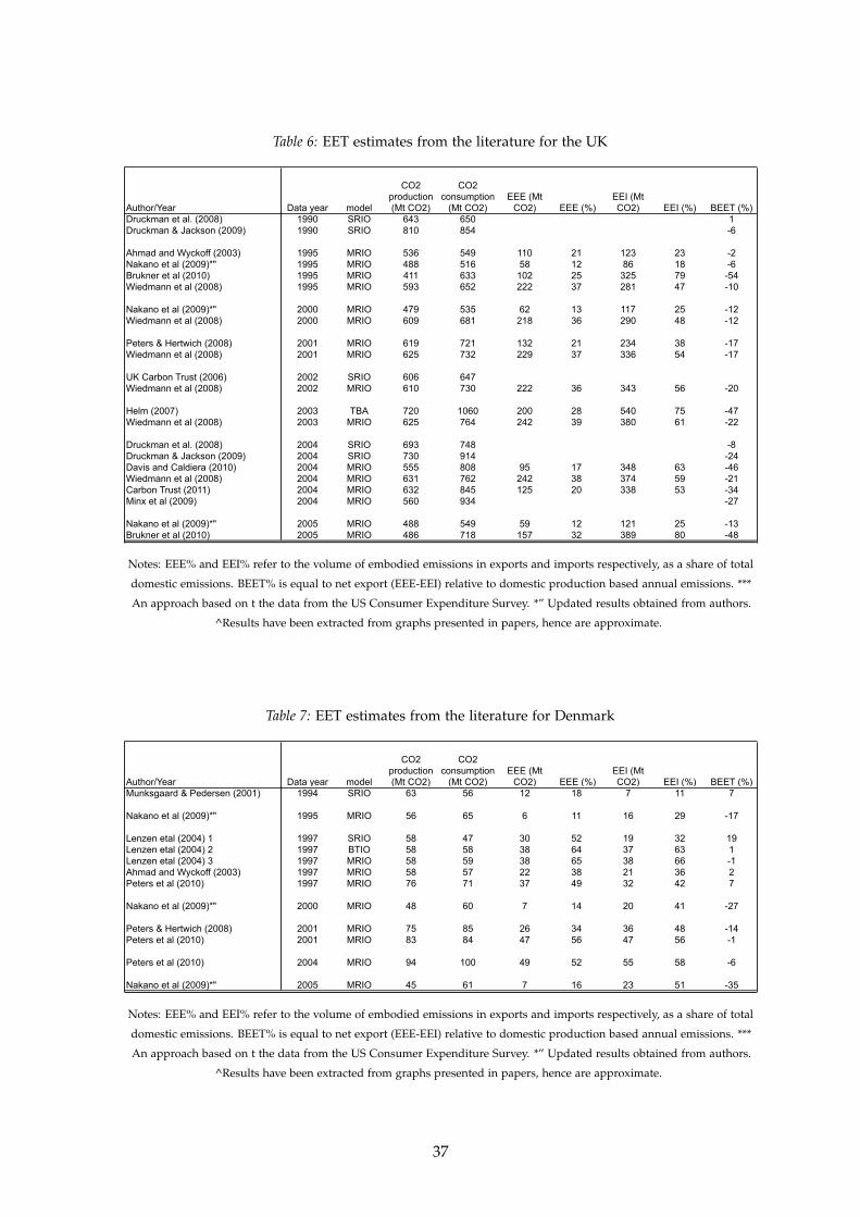
Table 6: EET estimates from the literature for the UK



CO2 consumption

(Mt CO2)EEE (Mt


Druckman et al. (2008) 1990 SRIO 643 650 1Druckman & Jackson (2009) 1990 SRIO 810 854 -6

Ahmad and Wyckoff (2003) 1995 MRIO 536 549 110 21 123 23 -2Nakano et al (2009)*" 1995 MRIO 488 516 58 12 86 18 -6Brukner et al (2010) 1995 MRIO 411 633 102 25 325 79 -54Wiedmann et al (2008) 1995 MRIO 593 652 222 37 281 47 -10

Nakano et al (2009)*" 2000 MRIO 479 535 62 13 117 25 -12Wiedmann et al (2008) 2000 MRIO 609 681 218 36 290 48 -12

Peters & Hertwich (2008) 2001 MRIO 619 721 132 21 234 38 -17Wiedmann et al (2008) 2001 MRIO 625 732 229 37 336 54 -17

UK Carbon Trust (2006) 2002 SRIO 606 647Wiedmann et al (2008) 2002 MRIO 610 730 222 36 343 56 -20

Helm (2007) 2003 TBA 720 1060 200 28 540 75 -47Wiedmann et al (2008) 2003 MRIO 625 764 242 39 380 61 -22

Druckman et al. (2008) 2004 SRIO 693 748 -8Druckman & Jackson (2009) 2004 SRIO 730 914 -24Davis and Caldiera (2010) 2004 MRIO 555 808 95 17 348 63 -46Wiedmann et al (2008) 2004 MRIO 631 762 242 38 374 59 -21Carbon Trust (2011) 2004 MRIO 632 845 125 20 338 53 -34Minx et al (2009) 2004 MRIO 560 934 -27

Nakano et al (2009)*" 2005 MRIO 488 549 59 12 121 25 -13Brukner et al (2010) 2005 MRIO 486 718 157 32 389 80 -48





Table 7: EET estimates from the literature for Denmark



CO2 consumption

(Mt CO2)EEE (Mt


Munksgaard & Pedersen (2001) 1994 SRIO 63 56 12 18 7 11 7

Nakano et al (2009)*" 1995 MRIO 56 65 6 11 16 29 -17

Lenzen etal (2004) 1 1997 SRIO 58 47 30 52 19 32 19Lenzen etal (2004) 2 1997 BTIO 58 58 38 64 37 63 1Lenzen etal (2004) 3 1997 MRIO 58 59 38 65 38 66 -1Ahmad and Wyckoff (2003) 1997 MRIO 58 57 22 38 21 36 2Peters et al (2010) 1997 MRIO 76 71 37 49 32 42 7

Nakano et al (2009)*" 2000 MRIO 48 60 7 14 20 41 -27

Peters & Hertwich (2008) 2001 MRIO 75 85 26 34 36 48 -14Peters et al (2010) 2001 MRIO 83 84 47 56 47 56 -1

Peters et al (2010) 2004 MRIO 94 100 49 52 55 58 -6

Nakano et al (2009)*" 2005 MRIO 45 61 7 16 23 51 -35





37

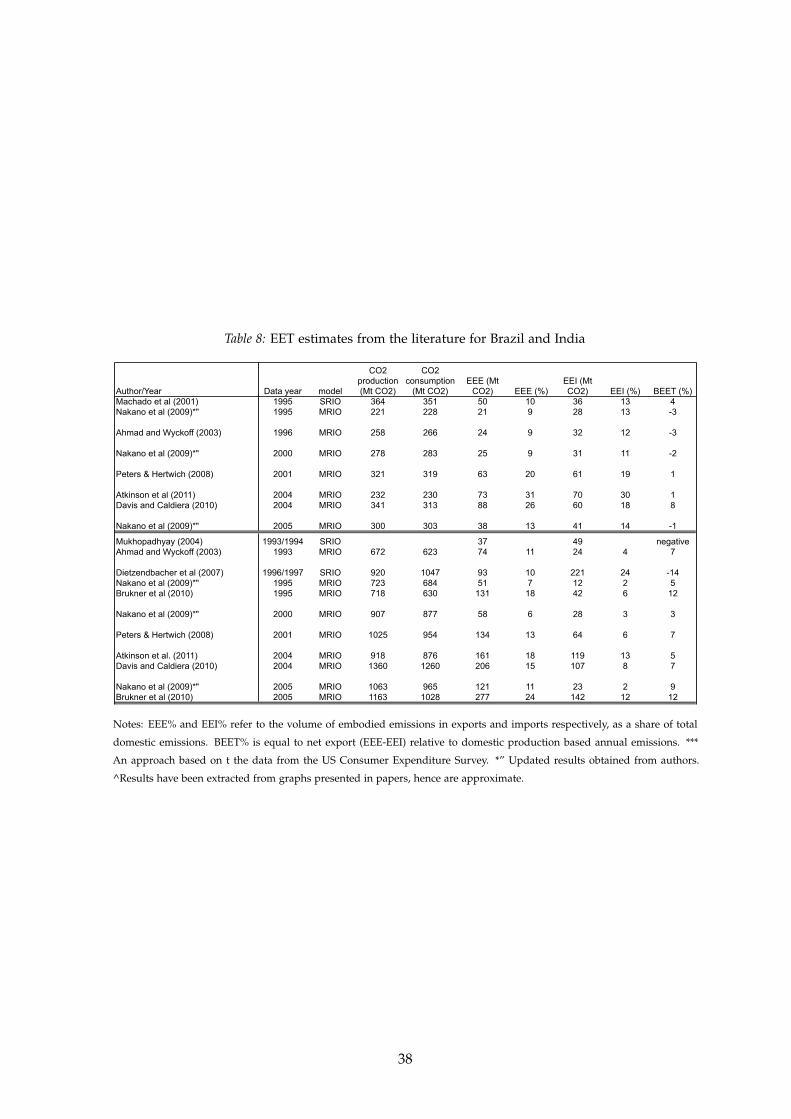
Table 8: EET estimates from the literature for Brazil and India



CO2 consumption

(Mt CO2)EEE (Mt


Machado et al (2001) 1995 SRIO 364 351 50 10 36 13 4Nakano et al (2009)*" 1995 MRIO 221 228 21 9 28 13 -3

Ahmad and Wyckoff (2003) 1996 MRIO 258 266 24 9 32 12 -3

Nakano et al (2009)*" 2000 MRIO 278 283 25 9 31 11 -2

Peters & Hertwich (2008) 2001 MRIO 321 319 63 20 61 19 1

Atkinson et al (2011) 2004 MRIO 232 230 73 31 70 30 1Davis and Caldiera (2010) 2004 MRIO 341 313 88 26 60 18 8

Nakano et al (2009)*" 2005 MRIO 300 303 38 13 41 14 -1

Mukhopadhyay (2004) 1993/1994 SRIO 37 49 negativeAhmad and Wyckoff (2003) 1993 MRIO 672 623 74 11 24 4 7

Dietzendbacher et al (2007) 1996/1997 SRIO 920 1047 93 10 221 24 -14Nakano et al (2009)*" 1995 MRIO 723 684 51 7 12 2 5Brukner et al (2010) 1995 MRIO 718 630 131 18 42 6 12

Nakano et al (2009)*" 2000 MRIO 907 877 58 6 28 3 3

Peters & Hertwich (2008) 2001 MRIO 1025 954 134 13 64 6 7

Atkinson et al. (2011) 2004 MRIO 918 876 161 18 119 13 5Davis and Caldiera (2010) 2004 MRIO 1360 1260 206 15 107 8 7

Nakano et al (2009)*" 2005 MRIO 1063 965 121 11 23 2 9Brukner et al (2010) 2005 MRIO 1163 1028 277 24 142 12 12





38

Tabl

e9:

Sum

mar

yof

met

hods

,dat

aan

dre

sults

from

13st

udie

sof

embo

died

emis

sion

sin

Chi

na’s

trad

efo

rth

eye

ars

2004

or20

05

Mod

el

refe

renc

eC

ount

ryYe

arst

ruct

ure

Eco

nom

ic

data

Trad

e D

ata

Em

isio

ns

Dat

a

sour

ceso

urce

sour

ce

#production sectors

#regions

#energy types

process emissions

international transport

service sectors

Exc

hang

e ra

tes

fore

ign

tech

nolo

gy

Feed

-ba

ck

Loop

IEA

(200

8)20

06%

exp

ort i

n G

DP

UN

CTA

D

IEA

Wor

ld

Ene

rgy

Sta

ts

& B

alan

ces

8ye

sn/

a

Wan

g &

W

atso

n (2

008)

Chi

na v

s

RO

W20

04tra

de

bala

nce

NB

S

IEA

CO

2 em

issi

ons

from

fuel

co

mbu

stio

nac

tual

term

sno

Web

er e

t al

(200

8)C

hina

vs

RO

W19

87-

2005

SR

ION

BS

for 1

997-

2005

GTA

P fo

r 198

7-20

02, C

hina

S

tatis

tical

Yea

r B

ook

for 2

005

from

Pet

ers,

W

eber

, Liu

(2

006)

422

20ye

sno

yes

n/a

impo

rt su

bstit

utio

n as

sum

ptio

nno

Pan

et a

l (2

008)

Chi

na v

s R

OW

2002

-20

06S

RIO

NB

SU

NC

OM

TRA

DE

Chi

na

Sta

tistic

al

Year

Boo

k37

2

impo

rt su

b.

adju

sted

by

natio

nal a

vg

inte

nsity

sca

lar

Hui

min

& Y

e (2

010)

Chi

na v

s R

OW

1997

-20

07S

RIO

NB

SIn

put-

outp

ut ta

bels

of

Chi

na, 2

002

NB

S F

orei

gn E

con

Sta

t Yrb

ook

1998

-20

05, G

TAP

(impo

rts)

IEA

CO

2 em

is. f

rom

fu

el c

ombu

st.

Yan

& Y

ang

(201

0)C

hina

vs

RO

W19

97-

2007

SR

IO

NB

S C

hina

in

put-o

utpu

t ta

ble,

199

7C

hine

se S

tatis

tical

Ye

arbo

ok

from

Pet

ers,

W

eber

, Liu

(2

006)

20ye

sno

yes

Chi

na's

ex

ports

ad

just

ed b

y P

PP

RO

W=

US

A (d

ata

from

C

arne

gie

Mel

lon

Uni

.GD

I)no

Lin

& S

un

(201

0)C

hina

vs

RO

W20

05B

TIO

NB

S

Chi

na

Sta

tistic

al

Year

Boo

k15

yes

adju

sted

Shi

mod

a et

al

(200

8)m

ultip

le20

00B

TIO

IED

Asi

an

inte

rnat

iona

l IO

da

ta

IED

Asi

an

inte

rnat

iona

l IO

da

ta

IEA

Wor

ld

Ene

rgy

Sta

ts

& B

alan

ces

1310

3no

yes

yes

yes

Nak

ano

et a

l (2

009)

mul

tiple

1995

, 20

00,

2005

MR

IO

OE

CD

ha

rmon

ised

IO

tabl

esO

EC

D B

ilate

ral

Trad

e da

taba

se

IEA

CO

2 em

is. f

rom

fu

el c

ombu

st.

1741

noye

sye

sM

ER

usin

g lik

e co

untri

esye

s

Bru

ckne

r et

al (2

010)

mul

tiple

1995

-20

05M

RIO

OE

CD

ha

rmon

ised

IO

tabl

esO

EC

D B

ilate

ral

Trad

e da

taba

seIE

A E

nerg

y ba

lanc

es48

554

noye

sye

sus

ing

like

coun

tries

yes

Pet

ers

&

Her

twic

h (2

008)

mul

tiple

2001

MR

IOG

TAP

6G

TAP

6G

TAP

5787

yes

Dav

is &

C

alde

ira

(201

0)m

ultip

le20

04M

RIO

GTA

P 7

GTA

P 7

GTA

P,

mat

ched

with

C

DIA

C57

113

yes

noA

tkin

son

et

al (2

011)

mul

tiple

2004

MR

IOG

TAP

7G

TAP

GTA

P19

15no

ME

Rye

s

Dat

aA

ssum

ptio

ns

Agg

rega

tion

Cov

erag

e

Not

e:Th

ere

sults

colu

mn

show

the

valu

esof

embo

died

emis

sion

ses

timat

eby

the

stud

ies,

inte

rms

ofth

eth

eto

tale

mis

sion

sat

trib

utab

leto

Chi

na’s

prod

uctio

n,co

nsum

ptio

n,ex

port

san

dim

port

s.

Embo

died

emis

sion

sin

expo

rts

(EEE

)and

impo

rts

(EEI

)are

pres

ente

dbo

thin

term

sof

the

abso

lute

volu

me

(inM

tCO

2)an

din

term

sof

ash

are

ofto

tale

mis

sion

sfr

ompr

oduc

tion

inC

hina

.**

Thes

e

valu

esw

ere

repo

rted

for

the

year

2006

.Par

tialM

RIO

mod

els

like

half-

way

betw

een

BTIO

and

MR

IO.T

hey

use

coun

try-

spec

ific

emis

sion

fact

oran

dm

ake

som

ead

just

men

tfor

re-e

xpor

ts.

39

Embodied carbon in trade: a survey of the empirical literature · Embodied carbon in trade: A...

Documents

Transcript of Embodied carbon in trade: a survey of the empirical literature · Embodied carbon in trade: A...