
Embedded Systems and Software Ed F. Deprettere, Todor Stefanov, Hristo Nikolov {edd, stefanov,...
76
Embedded Systems and Software Ed F. Deprettere, Todor Stefanov, Hristo Nikolov {edd, stefanov, nikolov}@liacs.nl Leiden Embedded Research Center Spring 2010; http://www.liacs.nl/~cserc/EMBSYST/ ESSOFIA2010
-
Upload
kenyon-shackleton -
Category
Documents
-
view
231 -
download
2
Transcript of Embedded Systems and Software Ed F. Deprettere, Todor Stefanov, Hristo Nikolov {edd, stefanov,...

Embedded Systems and Software
Ed F. Deprettere, Todor Stefanov, Hristo Nikolov{edd, stefanov, nikolov}@liacs.nl
Leiden Embedded Research CenterSpring 2010;
http://www.liacs.nl/~cserc/EMBSYST/ESSOFIA2010
Part II Process Networks
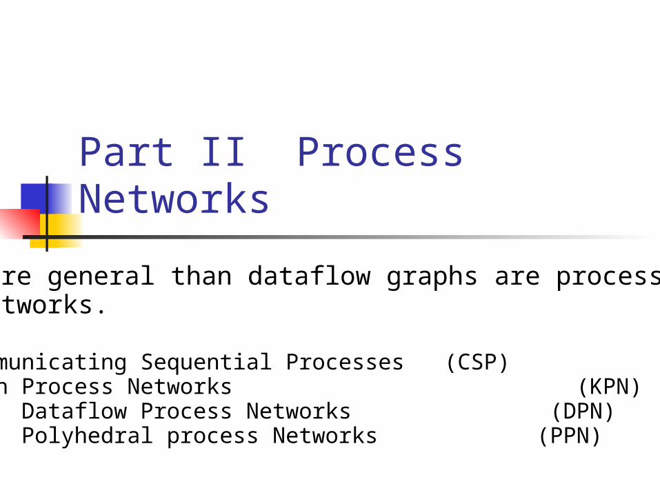
More general than dataflow graphs are processnetworks.
Communicating Sequential Processes (CSP)Kahn Process Networks (KPN) Dataflow Process Networks (DPN) Polyhedral process Networks (PPN)
What is the difference
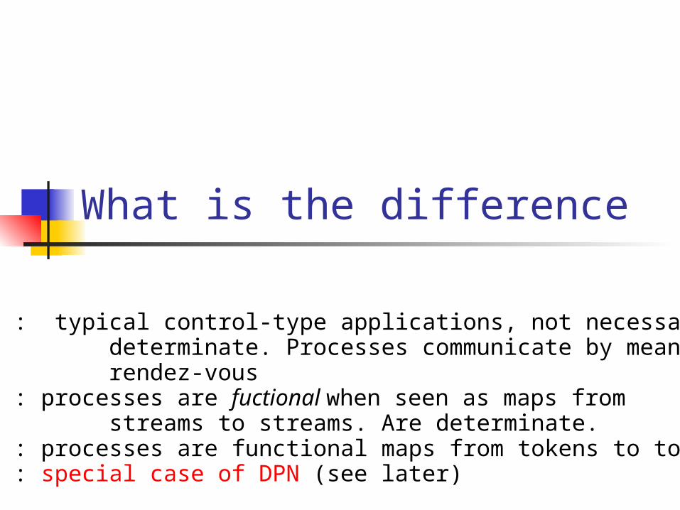
CSP : typical control-type applications, not necessarily determinate. Processes communicate by means of rendez-vousKPN : processes are fuctional when seen as maps from streams to streams. Are determinate.DPN : processes are functional maps from tokens to tokensPPN : special case of DPN (see later)
04/18/23 04ESSOFIA
Usage of KPNs
The KPN model of computation is used to specify applications in aconcurrent language.
Processes are specified in a host language (C, C++, Java). Thecommunication between processes is specified in a co-ordinationlanguage: blocking read.
KPN is a convenient model for streaming data applications: audio,and video, multimedia in general.
Processes operate on infinite streams of date, one quantum of dataat a time, i.e., the streams need not be available as a whole.
04/18/23 04ESSOFIA
Dataflow and Kahn Process Networks
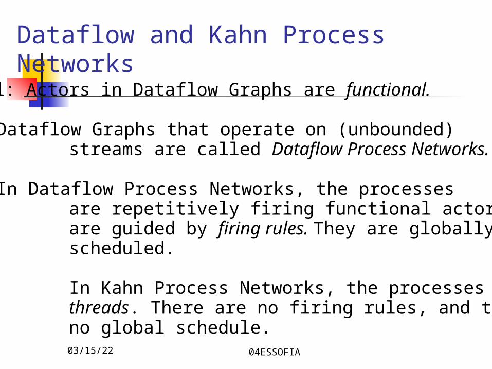
Recall: Actors in Dataflow Graphs are functional.
Dataflow Graphs that operate on (unbounded) streams are called Dataflow Process Networks.
In Dataflow Process Networks, the processes are repetitively firing functional actors that are guided by firing rules. They are globally scheduled.
In Kahn Process Networks, the processes are threads. There are no firing rules, and there is no global schedule.
04/18/23 04ESSOFIA
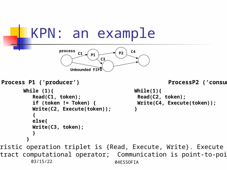
P2P1process
Unbounded FIFO
Process P1 (‘producer’) ProcessP2 (‘consumer’)
While (1){ Read(C1, token); if (token != Token) { Write(C2, Execute(token)); { else{ Write(C3, token); } }
C1
C3
While(1){ Read(C2, token); Write(C4, Execute(token));}
C4
Characteristic operation triplet is {Read, Execute, Write}. Execute refers tosome abstract computational operator; Communication is point-to-point.
KPN: an example
04/18/23 04ESSOFIA
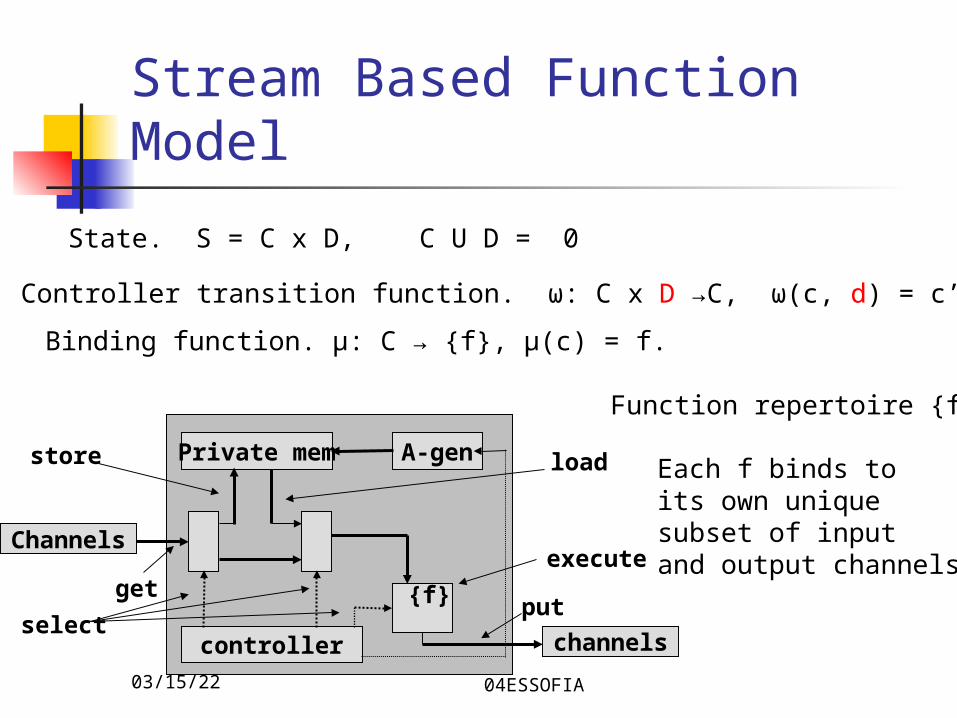
Stream Based Function Model
Private mem A-gen
{f}
controller
Channels
channels
store load
executeget
putselect
State. S = C x D, C U D = 0
Controller transition function. ω: C x D →C, ω(c, d) = c’
Binding function. μ: C → {f}, μ(c) = f.
Function repertoire {f}
Each f binds toits own uniquesubset of inputand output channels
04/18/23 04ESSOFIA
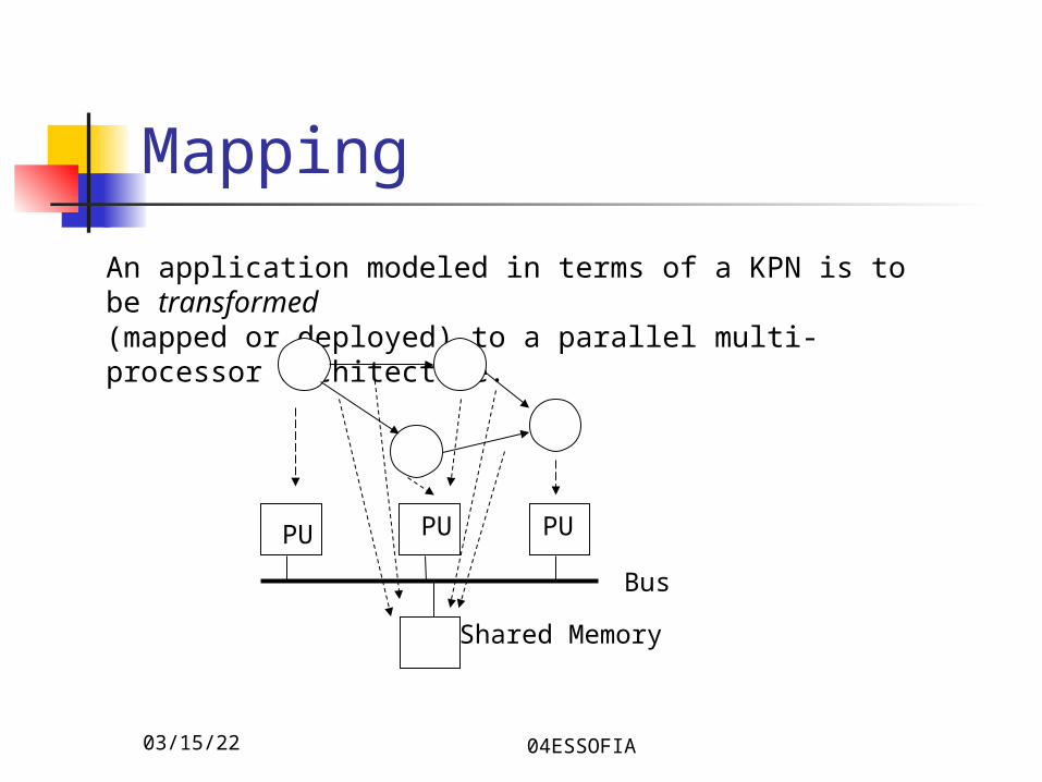
Mapping
An application modeled in terms of a KPN is to be transformed(mapped or deployed) to a parallel multi-processor architecture.
PU PU PU
Shared Memory
Bus
04/18/23 04ESSOFIA
Part II: applying it all
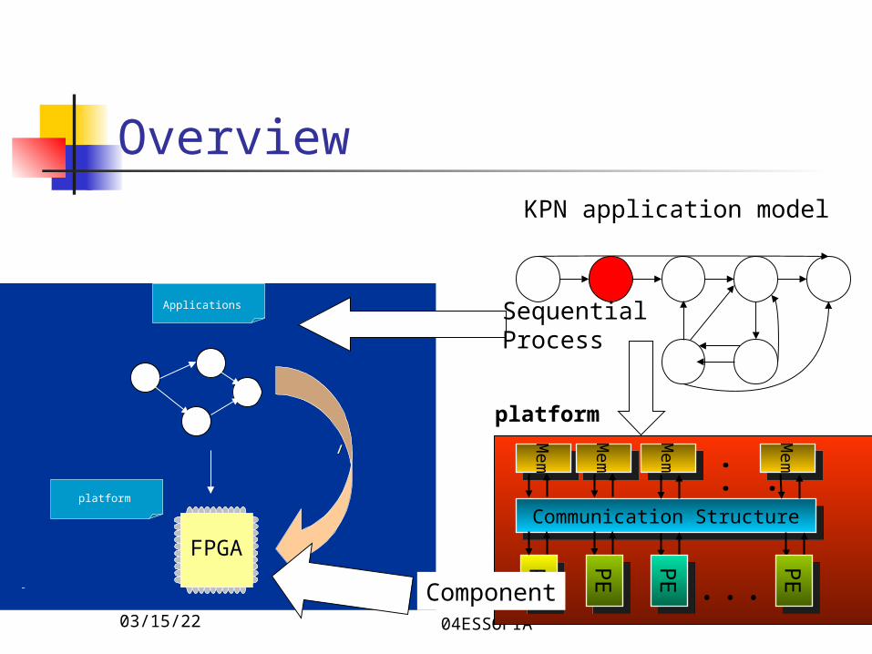
Overview
FPGA
Applications
–
/ /
platform
KPN application model
SequentialProcess
platform
Communication StructureCommunication Structure
Mem
Mem
PE
PE ...
.. .
PE
PE PE
PE PE
PE
Mem
Mem
Mem
Mem
Mem
Mem
Component
04/18/23 04ESSOFIA
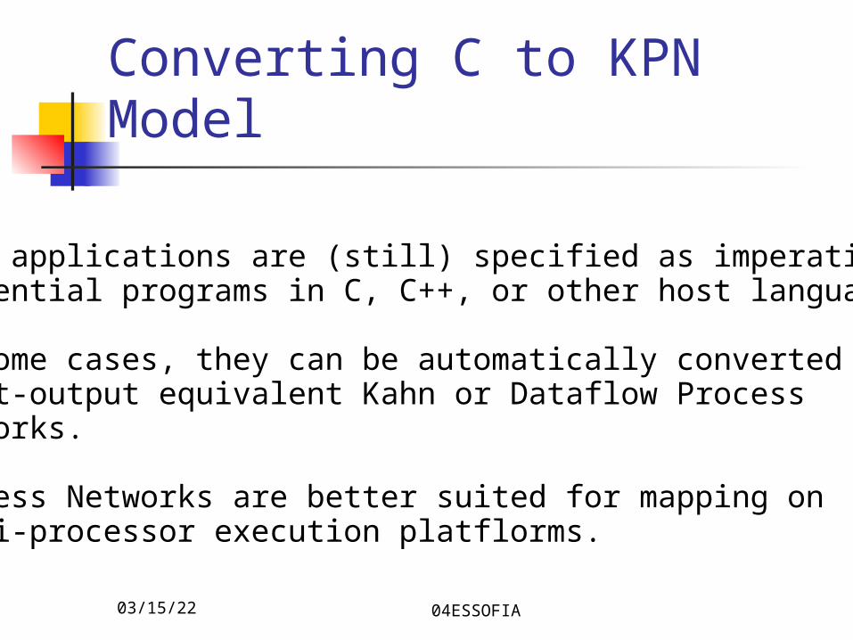
Converting C to KPN Model
Most applications are (still) specified as imperativesequential programs in C, C++, or other host languages.
In some cases, they can be automatically converted toinput-output equivalent Kahn or Dataflow ProcessNetworks.
Process Networks are better suited for mapping onmulti-processor execution platflorms.
04/18/23 04ESSOFIA
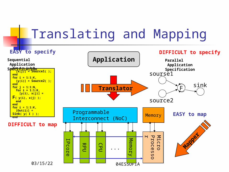
Translating and Mapping
Application
Programmable Interconnect (NoC)Programmable Interconnect (NoC)
IPcore
IPcore
RP
UR
PU
Mem
oryM
emory
CP
UC
PU
Micro
Processor
Micro
Processor
MemoryMemory
...
Programming
for j = 1:1:N, [x(j)] = Source1( ); endfor i = 1:1:K, [y(i)] = Source2( ); endfor j = 1:1:N, for i = 1:1:K,
[y(i), x(j)] = F( y(i), x(j) ); endendfor i = 1:1:K, [Out(i)] = Sink( y( I ) ); end
Sequential Application Specification
EASY to specify
DIFFICULT to map
Translator
Map
per
EASY to map
Parallel Application Specification
DIFFICULT to specify
F
sourse1
source2
sink
04/18/23 04ESSOFIA
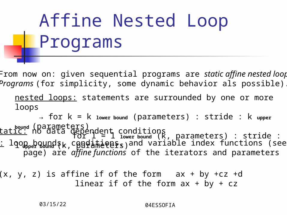
Affine Nested Loop Programs
From now on: given sequential programs are static affine nested loopPrograms (for simplicity, some dynamic behavior als possible).
nested loops: statements are surrounded by one or more loops → for k = k lower bound (parameters) : stride : k upper bound (parameters) for l = l lower bound (k, parameters) : stride : l upper bound (k, parameters) static: no data dependent conditions
affine: loop bounds, conditions, and variable index functions (see next page) are affine functions of the iterators and parameters
f(x, y, z) is affine if of the form ax + by +cz +d linear if of the form ax + by + cz
04/18/23 04ESSOFIA
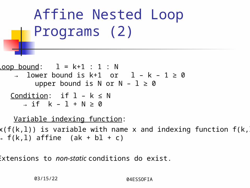
Affine Nested Loop Programs (2)
Loop bound: l = k+1 : 1 : N → lower bound is k+1 or l – k – 1 ≥ 0 upper bound is N or N – l ≥ 0
Condition: if l – k ≤ N → if k – l + N ≥ 0
Variable indexing function:
x(f(k,l)) is variable with name x and indexing function f(k,l)→ f(k,l) affine (ak + bl + c)
Extensions to non-static conditions do exist.
04/18/23 04ESSOFIA
Extensions
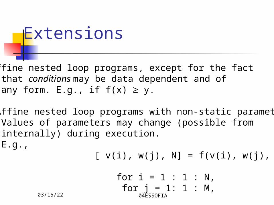
1. Affine nested loop programs, except for the fact that conditions may be data dependent and of any form. E.g., if f(x) ≥ y.
2. Affine nested loop programs with non-static parameters. Values of parameters may change (possible from internally) during execution. E.g., [ v(i), w(j), N] = f(v(i), w(j), M); for i = 1 : 1 : N, for j = 1: 1 : M,
04/18/23 04ESSOFIA
Affine Nested Loop Programs (3)
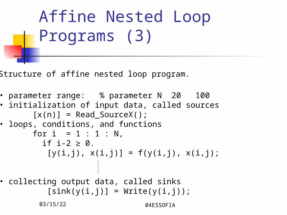
Structure of affine nested loop program.
• parameter range: % parameter N 20 100• initialization of input data, called sources [x(n)] = Read_SourceX();• loops, conditions, and functions for i = 1 : 1 : N, if i-2 ≥ 0. [y(i,j), x(i,j)] = f(y(i,j), x(i,j);
• collecting output data, called sinks [sink(y(i,j)] = Write(y(i,j));
04/18/23 04ESSOFIA
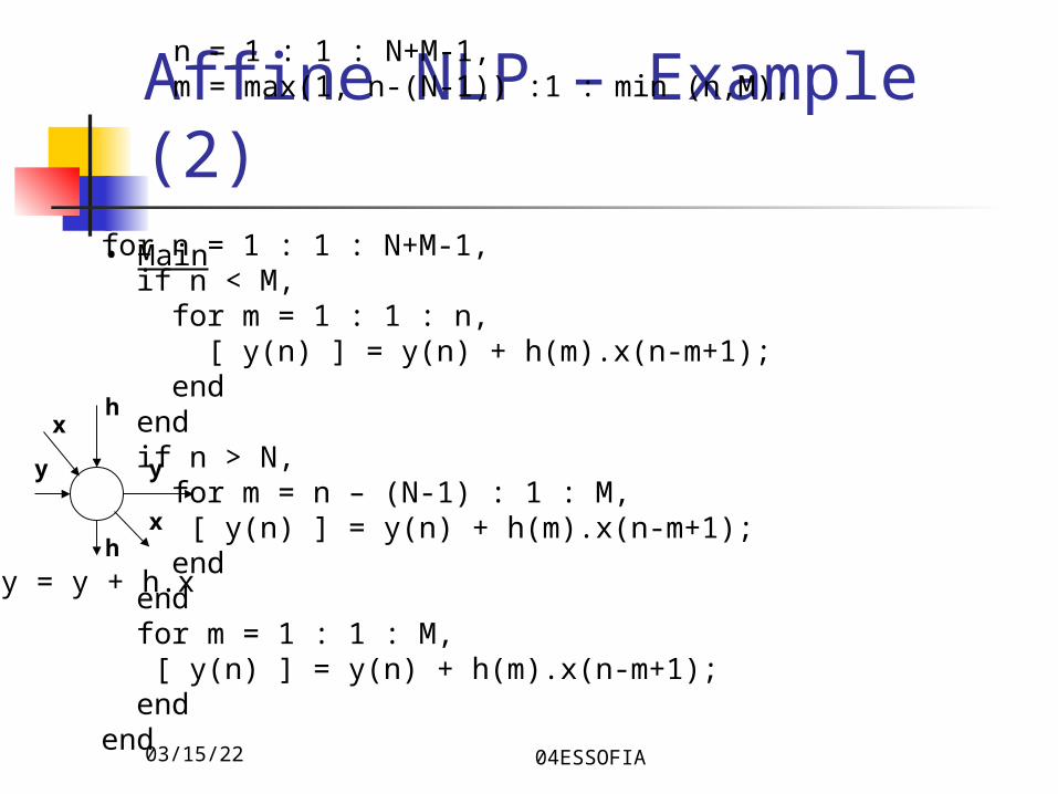
Affine NLP – Example (2)• Main for n = 1 : 1 : N+M-1,
if n < M, for m = 1 : 1 : n, [ y(n) ] = y(n) + h(m).x(n-m+1); end end if n > N, for m = n – (N-1) : 1 : M, [ y(n) ] = y(n) + h(m).x(n-m+1); end end for m = 1 : 1 : M, [ y(n) ] = y(n) + h(m).x(n-m+1); endend
y y
h
h
x
x
y = y + h.x
n = 1 : 1 : N+M-1,m = max(1, n-(N-1)) :1 : min (n,M),
04/18/23 04ESSOFIA
From ANLP to KPN
• Converting ANLPs to input/output equivalent KPNs provides (equivalent) concurrent processing specifications that facilitate mapping onto parallel architectures
• Because ANLPs are static, the corresponding KPNs are also static. They are in some sense similar to Cyclo-Static dataflow process networks.
• Global schedules can be derived, and sizes of buffers can be determined, at least an upper bound for them.
04/18/23 04ESSOFIA
From ANLP to PN (2)
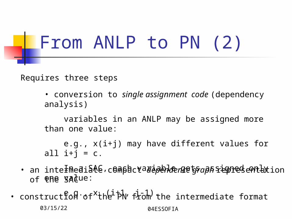
Requires three steps
• conversion to single assignment code (dependency analysis)
variables in an ANLP may be assigned more than one value:
e.g., x(i+j) may have different values for all i+j = c.
In a SAC, each variable gets assigned only one value:
e.g., x1 (i+1, j-1).
• an intermediate compact dependence graph representation of the SAC
• construction of the PN from the intermediate format
04/18/23 04ESSOFIA
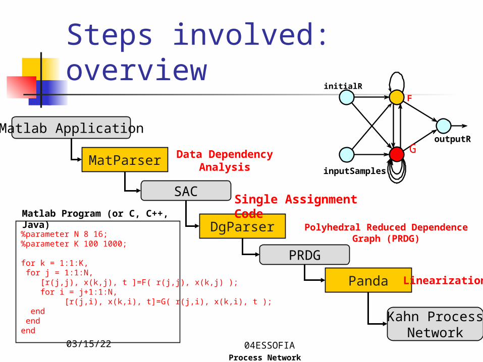
Steps involved: overview
%parameter N 8 16;%parameter K 100 1000;
for k = 1:1:K, for j = 1:1:N, [r(j,j), x(k,j), t ]=F( r(j,j), x(k,j) ); for i = j+1:1:N, [r(j,i), x(k,i), t]=G( r(j,i), x(k,i), t ); end endend
Matlab Program (or C, C++, Java)
Matlab Application
Process Network
Kahn ProcessNetwork
DgParser
PRDG
Polyhedral Reduced Dependence Graph (PRDG)
MatParser Data DependencyAnalysis
Panda Linearization
outputR
F
initialR
inputSamples
G
SACSingle Assignment Code
04/18/23 04ESSOFIA
Data Dependency Analysisj
1 2 3 4 5 N=612
43
5N=6
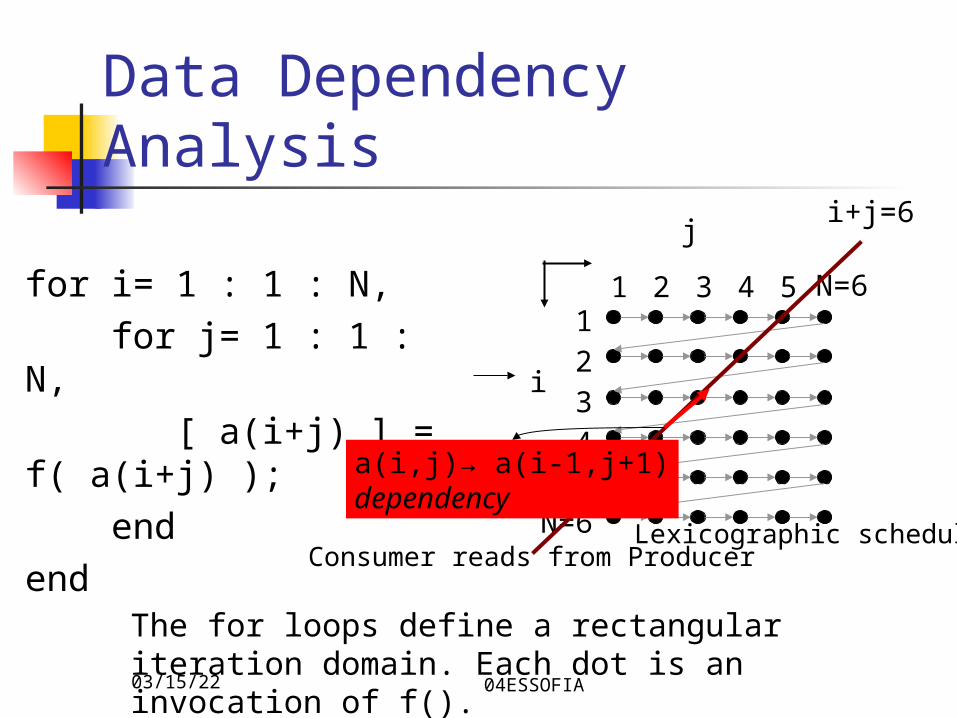
for i= 1 : 1 : N, for j= 1 : 1 : N, [ a(i+j) ] = f( a(i+j) ); endend
The for loops define a rectangular iteration domain. Each dot is an invocation of f().
i
i+j=6
a(i,j)→ a(i-1,j+1)dependency
Consumer reads from ProducerLexicographic schedule
04/18/23 04ESSOFIA
Data Dependency Analysis (2)
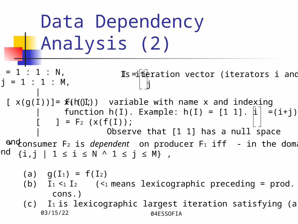
i = 1 : 1 : N, j = 1 : 1 : M, | [ x(g(I))]= F1 (); | [ ] = F2 (x(f(I)); | endend
x(h(I)) variable with name x and indexingfunction h(I). Example: h(I) = [1 1]. i =(i+j) j
• consumer F2 is dependent on producer F1 iff - in the domain {i,j | 1 ≤ i ≤ N ^ 1 ≤ j ≤ M} ,
(a) g(I1) = f(I2) (b) I1 <l I2 (<l means lexicographic preceding = prod. before cons.) (c) I1 is lexicographic largest iteration satisfying (a) and (b)
Observe that [1 1] has a null space
I = i j
Is iteration vector (iterators i and j)
04/18/23 04ESSOFIA
Data Dependency Analysis (3)
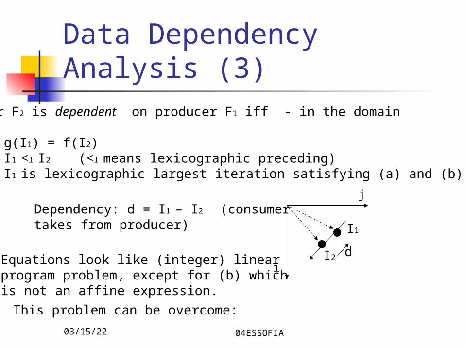
consumer F2 is dependent on producer F1 iff - in the domain
(a) g(I1) = f(I2) (b) I1 <l I2 (<l means lexicographic preceding) (c) I1 is lexicographic largest iteration satisfying (a) and (b)
Dependency: d = I1 – I2 (consumertakes from producer)
j
i
I1
I2 dEquations look like (integer) linearprogram problem, except for (b) whichis not an affine expression.
This problem can be overcome:
04/18/23 04ESSOFIA
Data Dependency Analysis (4)
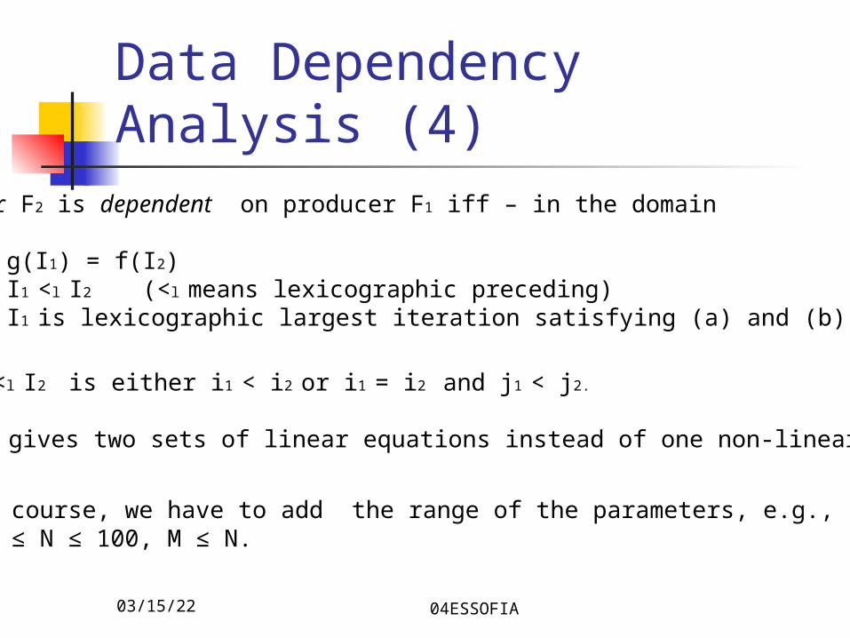
consumer F2 is dependent on producer F1 iff – in the domain
(a) g(I1) = f(I2) (b) I1 <l I2 (<l means lexicographic preceding) (c) I1 is lexicographic largest iteration satisfying (a) and (b)
I1 <l I2 is either i1 < i2 or i1 = i2 and j1 < j2.
This gives two sets of linear equations instead of one non-linear set.
Of course, we have to add the range of the parameters, e.g., 30 ≤ N ≤ 100, M ≤ N.
04/18/23 04ESSOFIA
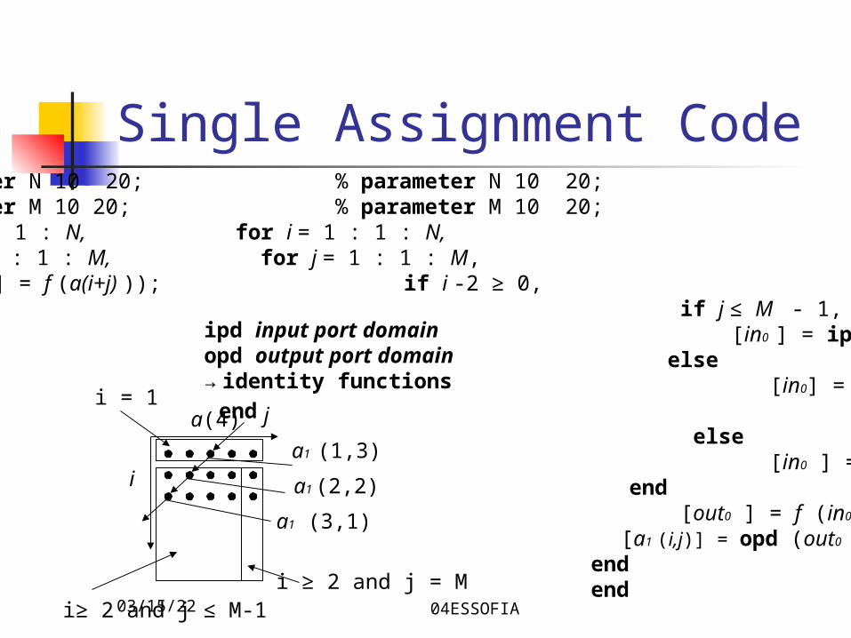
Single Assignment Code% parameter N 10 20; % parameter N 10 20;% parameter M 10 20; % parameter M 10 20;for i = 1 : 1 : N, for i = 1 : 1 : N, for j = 1 : 1 : M, for j = 1 : 1 : M, [ a(i+j)] = f (a(i+j) )); if i -2 ≥ 0, end if j ≤ M - 1,end [in0 ] = ipd (a1 (i -1, j +1)); else [in0] = ipd (a (i + j)); end else [in0 ] = ipd (a (i + j)); end [out0 ] = f (in0 ); [a1 (i,j)] = opd (out0 ); end end
ja(4)
ia1 (1,3)
a1 (2,2)
a1 (3,1)
i≥ 2 and j ≤ M-1i ≥ 2 and j = M
i = 1
ipd input port domainopd output port domain→ identity functions
04/18/23 04ESSOFIA
Polyhedron
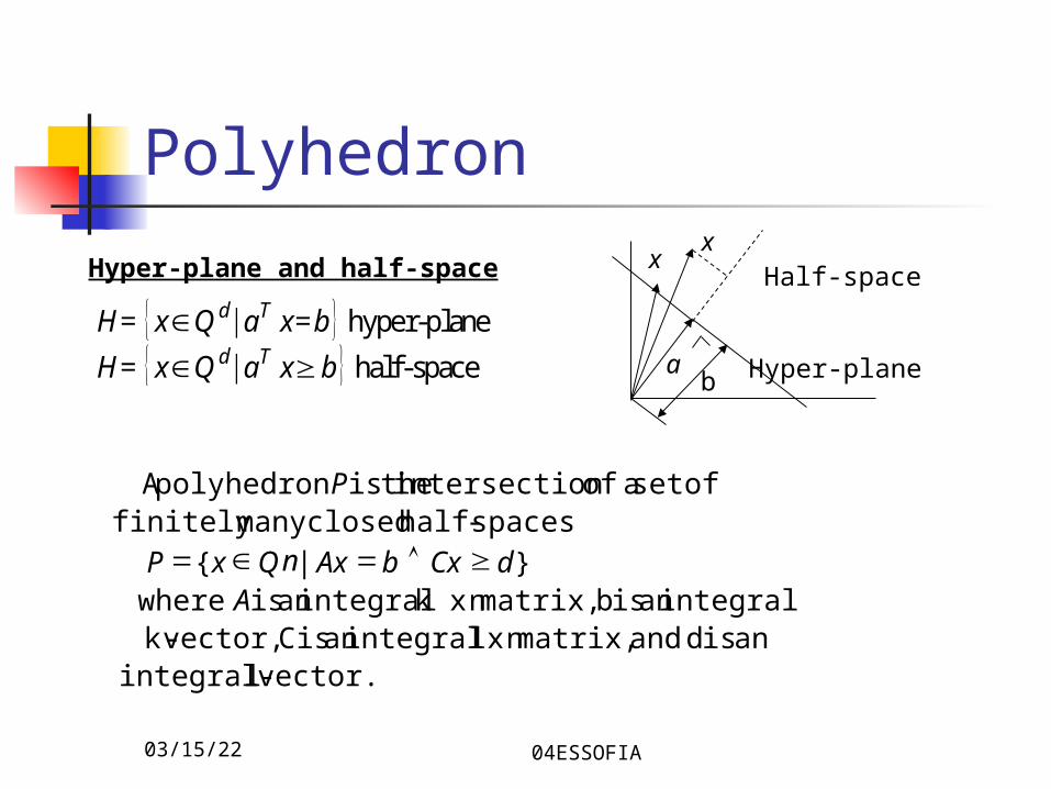
Hyper-plane and half-space
H= { x∈Q d∣aT x=b } hyper-plane
H= { x∈Q d∣aT x≥b } half-space
x
a
x
b Hyper-plane
Half-space
vector.-l integralan is d and matrix,n x l integralan is C vector,-k
integralan is b matrix,n k x integralan is where}|{
spaces-half closedmany finitely ofset a of intersection theis polyhedronA
AdCxbAxQxP
P
n
04/18/23 04ESSOFIA
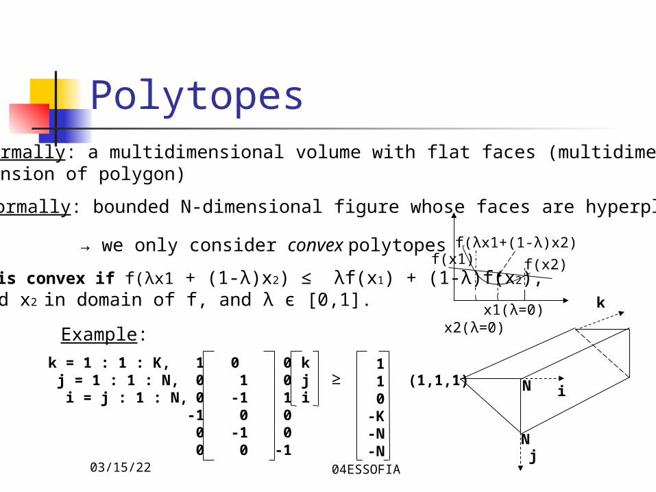
PolytopesInformally: a multidimensional volume with flat faces (multidimensionalextension of polygon)
Formally: bounded N-dimensional figure whose faces are hyperplanes
Example:
k = 1 : 1 : K, j = 1 : 1 : N, i = j : 1 : N,
1 0 0 0 1 0 0 -1 1-1 0 0 0 -1 0 0 0 -1
kji
≥ 1 1 0-K-N-N
k
j
iN
N
(1,1,1)
→ we only consider convex polytopes
f(x) is convex if f(λx1 + (1-λ)x2) ≤ λf(x1) + (1-λ)f(x2),x1 and x2 in domain of f, and λ є [0,1]. x1(λ=0) x2(λ=0)
f(x1) f(x2)
f(λx1+(1-λ)x2)
04/18/23 04ESSOFIA
Polytopes(2)
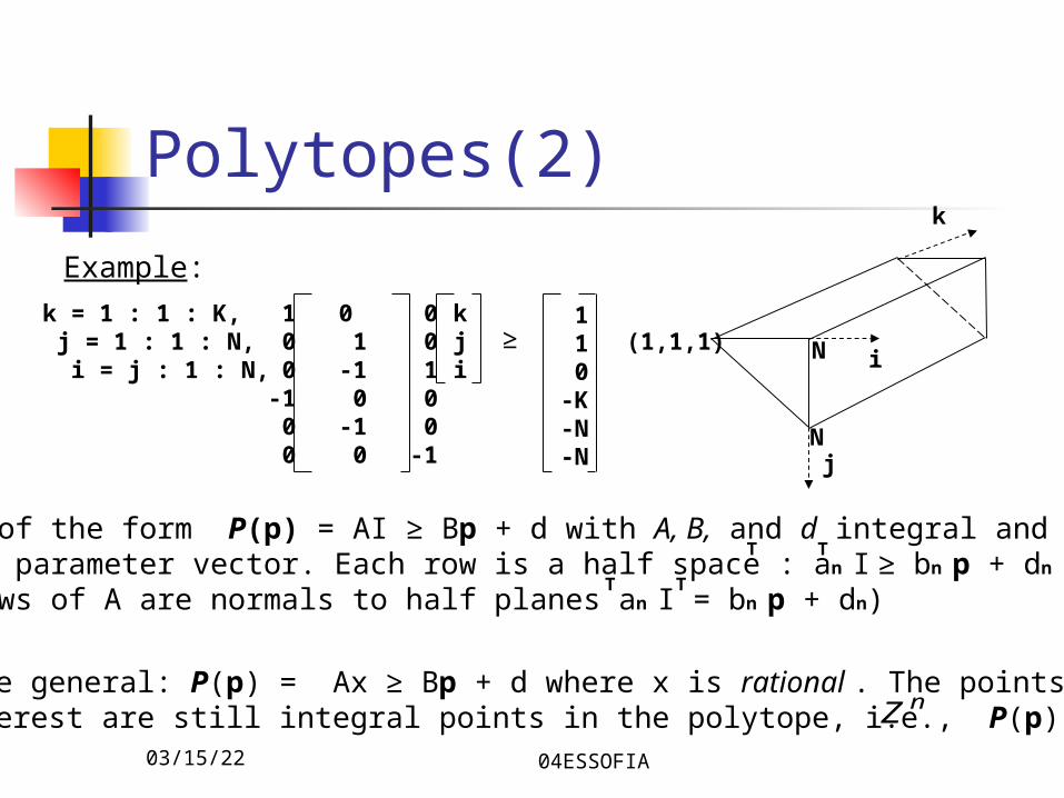
Example:
k = 1 : 1 : K, j = 1 : 1 : N, i = j : 1 : N,
1 0 0 0 1 0 0 -1 1-1 0 0 0 -1 0 0 0 -1
kji
≥ 1 1 0-K-N-N
k
j
iN
N
(1,1,1)
More general: P(p) = Ax ≥ Bp + d where x is rational . The points of interest are still integral points in the polytope, i.e., P(p) ∩ Ζ
n
Is of the form P(p) = AI ≥ Bp + d with A, B, and d integral and pthe parameter vector. Each row is a half space : an I ≥ bn p + dn
(rows of A are normals to half planes an I = bn p + dn)
T T
T T
04/18/23 04ESSOFIA
Polytopes (3)
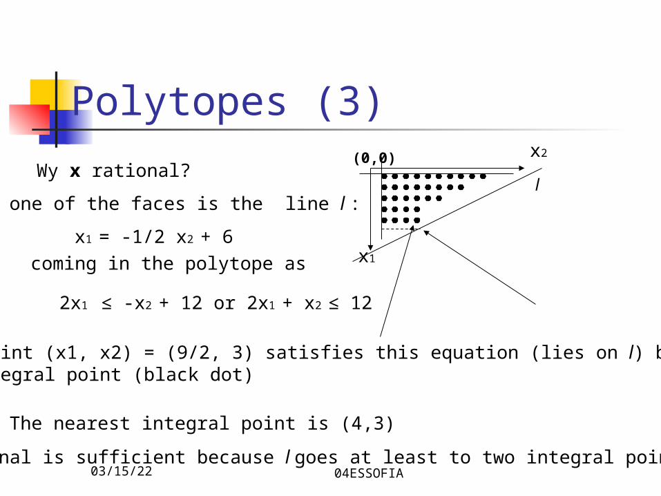
Wy x rational?
one of the faces is the line l :
x1 = -1/2 x2 + 6
coming in the polytope as
2x1 ≤ -x2 + 12 or 2x1 + x2 ≤ 12
the point (x1, x2) = (9/2, 3) satisfies this equation (lies on l) but is notan integral point (black dot)
The nearest integral point is (4,3)
Rational is sufficient because l goes at least to two integral points.
x1
x2(0,0)
l
04/18/23 04ESSOFIA
Example
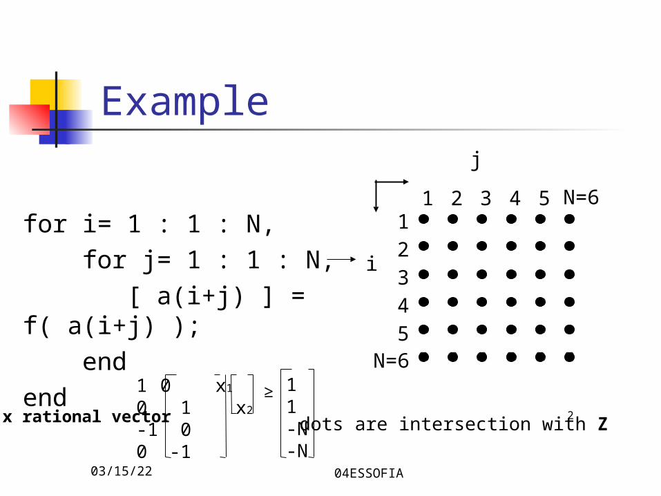
for i= 1 : 1 : N, for j= 1 : 1 : N, [ a(i+j) ] = f( a(i+j) ); endend
j
1 2 3 4 5 N=612
43
5N=6
i
1 0 x1
0 1 x2
-1 00 -1
≥ 11-N-N
dots are intersection with Z 2x rational vector
04/18/23 04ESSOFIA
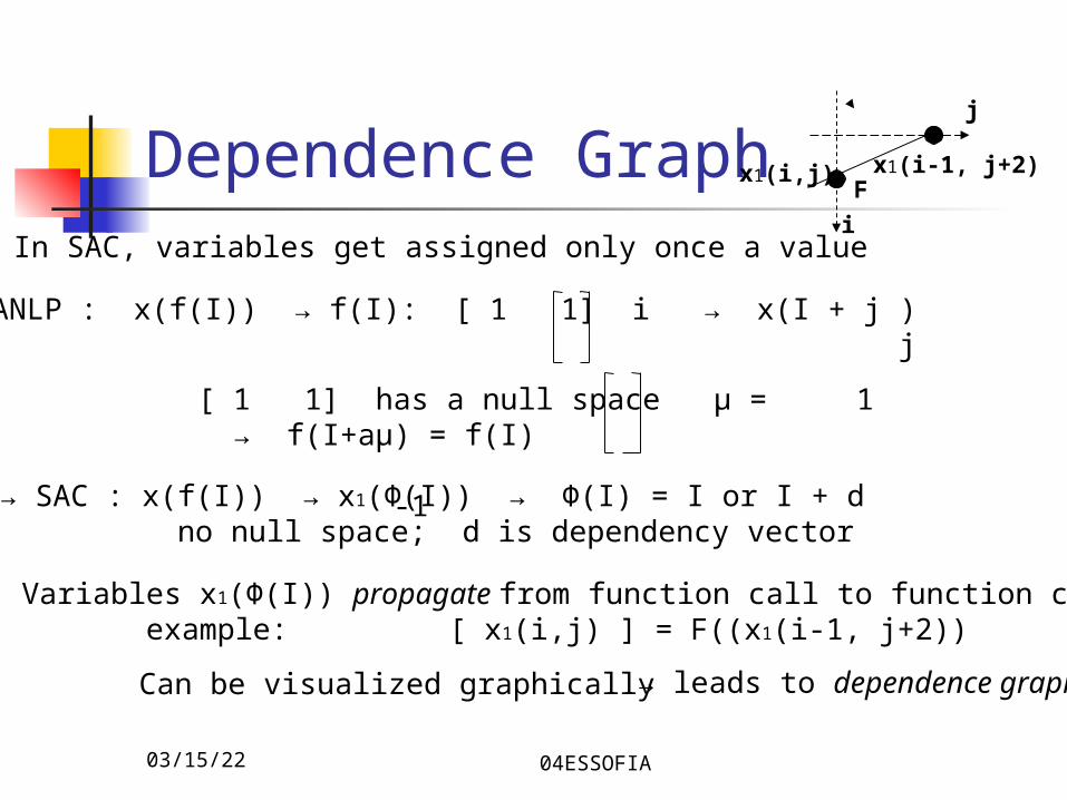
Dependence GraphIn SAC, variables get assigned only once a value
→ ANLP : x(f(I)) → f(I): [ 1 1] i → x(I + j ) j
[ 1 1] has a null space μ = 1 → f(I+aμ) = f(I) -1
→ SAC : x(f(I)) → x1(Φ(I)) → Φ(I) = I or I + d no null space; d is dependency vector
Variables x1(Φ(I)) propagate from function call to function call example: [ x1(i,j) ] = F((x1(i-1, j+2))
Fx1(i-1, j+2)x1(i,j)
i
j
Can be visualized graphically → leads to dependence graph
04/18/23 04ESSOFIA
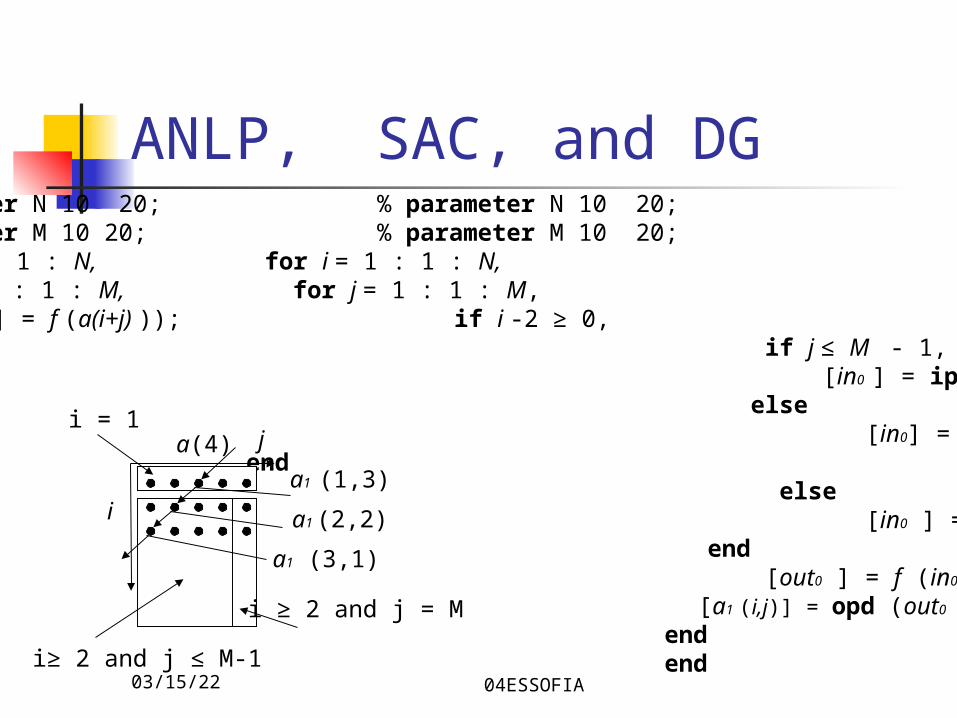
ANLP, SAC, and DG% parameter N 10 20; % parameter N 10 20;% parameter M 10 20; % parameter M 10 20;for i = 1 : 1 : N, for i = 1 : 1 : N, for j = 1 : 1 : M, for j = 1 : 1 : M, [ a(i+j)] = f (a(i+j) )); if i -2 ≥ 0, end if j ≤ M - 1,end [in0 ] = ipd (a1 (i -1, j +1)); else [in0] = ipd (a (i + j)); end else [in0 ] = ipd (a (i + j)); end [out0 ] = f (in0 ); [a1 (i,j)] = opd (out0 ); end endi≥ 2 and j ≤ M-1
ja(4)
ia1 (1,3)
a1 (2,2)
a1 (3,1)
i ≥ 2 and j = M
i = 1
04/18/23 04ESSOFIA
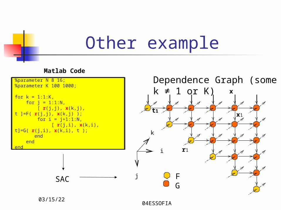
Other example
%parameter N 8 16;%parameter K 100 1000;
for k = 1:1:K, for j = 1:1:N, [ r(j,j), x(k,j), t ]=F( r(j,j), x(k,j) ); for i = j+1:1:N, [ r(j,i), x(k,i), t]=G( r(j,i), x(k,i), t ); end endend
Matlab Code
SAC
i
FG
Dependence Graph (somek ≠ 1 or K)
k
j
x
x1
r1
t1
04/18/23 04ESSOFIA
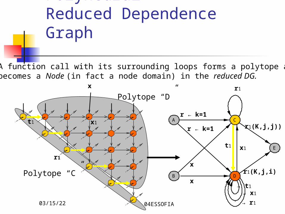
Polyhedral Reduced Dependence Graph
Polytope “C”
Polytope “D”
x
x1
r1
t1 CA
B D
E
r1
r ← k=1
r ← k=1
x
x
t1 x1
r1(K,j,j))
r1(K,j,i)
→ t1
→ x1
→ r1
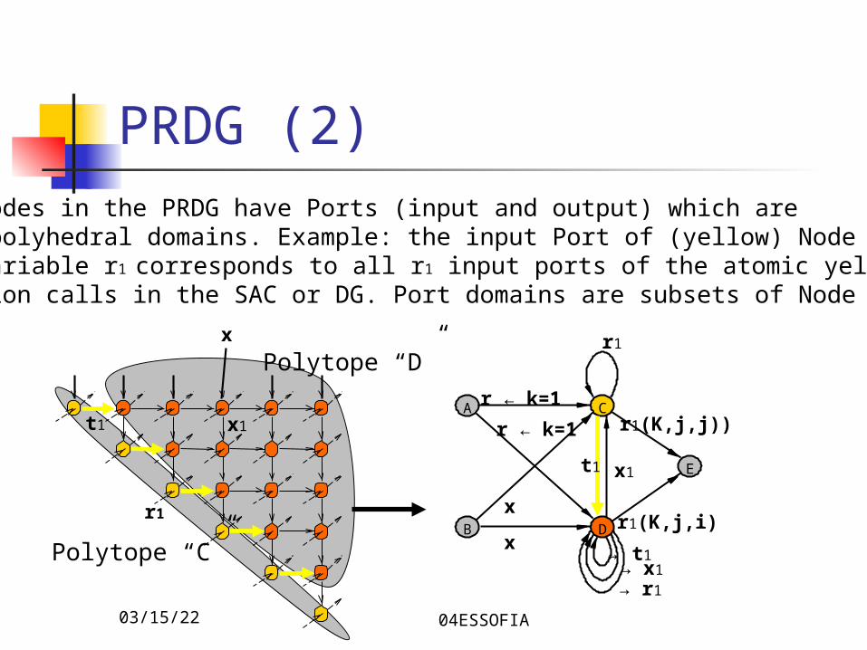
A function call with its surrounding loops forms a polytope and becomes a Node (in fact a node domain) in the reduced DG.
04/18/23 04ESSOFIA
PRDG (2)
CA
B D
E
r1
r ← k=1
r ← k=1
x
x
t1 x1
r1(K,j,j))
r1(K,j,i)
→ t1→ x1
→ r1
The Nodes in the PRDG have Ports (input and output) which arealso polyhedral domains. Example: the input Port of (yellow) Node Cfor variable r1 corresponds to all r1 input ports of the atomic yellowfunction calls in the SAC or DG. Port domains are subsets of Node domain
Polytope “C”
Polytope “D”x
x1
r1
t1
04/18/23 04ESSOFIA
PRDG (3)CA
B D
E
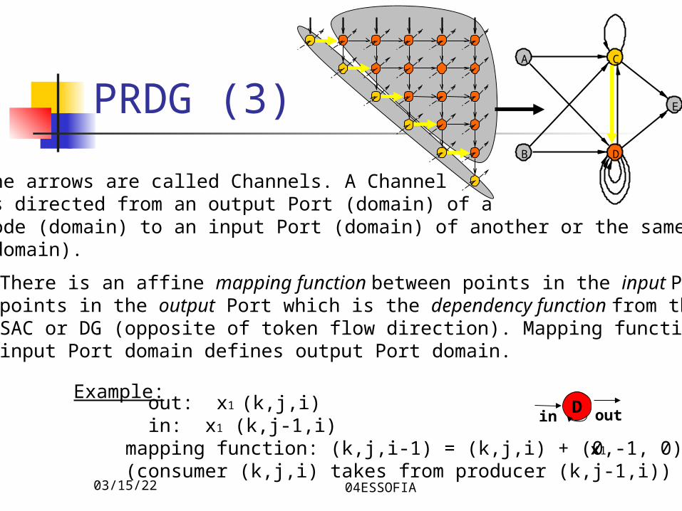
The arrows are called Channels. A Channelis directed from an output Port (domain) of aNode (domain) to an input Port (domain) of another or the same Node(domain).
There is an affine mapping function between points in the input Port topoints in the output Port which is the dependency function from theSAC or DG (opposite of token flow direction). Mapping function +input Port domain defines output Port domain.
out: x1 (k,j,i) in: x1 (k,j-1,i) mapping function: (k,j,i-1) = (k,j,i) + (0,-1, 0) (consumer (k,j,i) takes from producer (k,j-1,i))
Example:D
x1
in out
04/18/23 04ESSOFIA
PRDG (4)
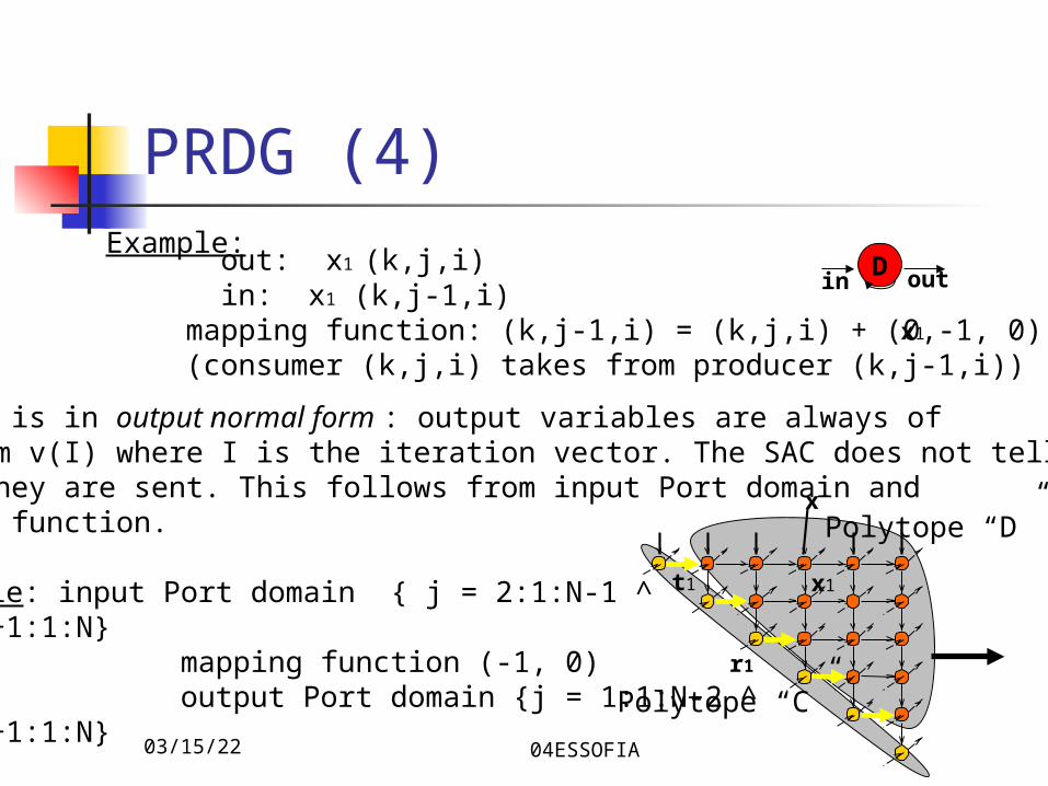
The SAC is in output normal form : output variables are always ofthe form v(I) where I is the iteration vector. The SAC does not tellwhere they are sent. This follows from input Port domain andmapping function.
Example: input Port domain { j = 2:1:N-1 ^i = j+1:1:N} mapping function (-1, 0) output Port domain {j = 1:1:N-2 ^I = j+1:1:N}
Polytope “C”
Polytope “D”x
x1
r1
t1
out: x1 (k,j,i) in: x1 (k,j-1,i) mapping function: (k,j-1,i) = (k,j,i) + (0,-1, 0) (consumer (k,j,i) takes from producer (k,j-1,i))
Example:D
x1
in out
04/18/23 04ESSOFIA
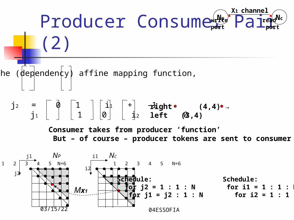
Producer Consumer Pair
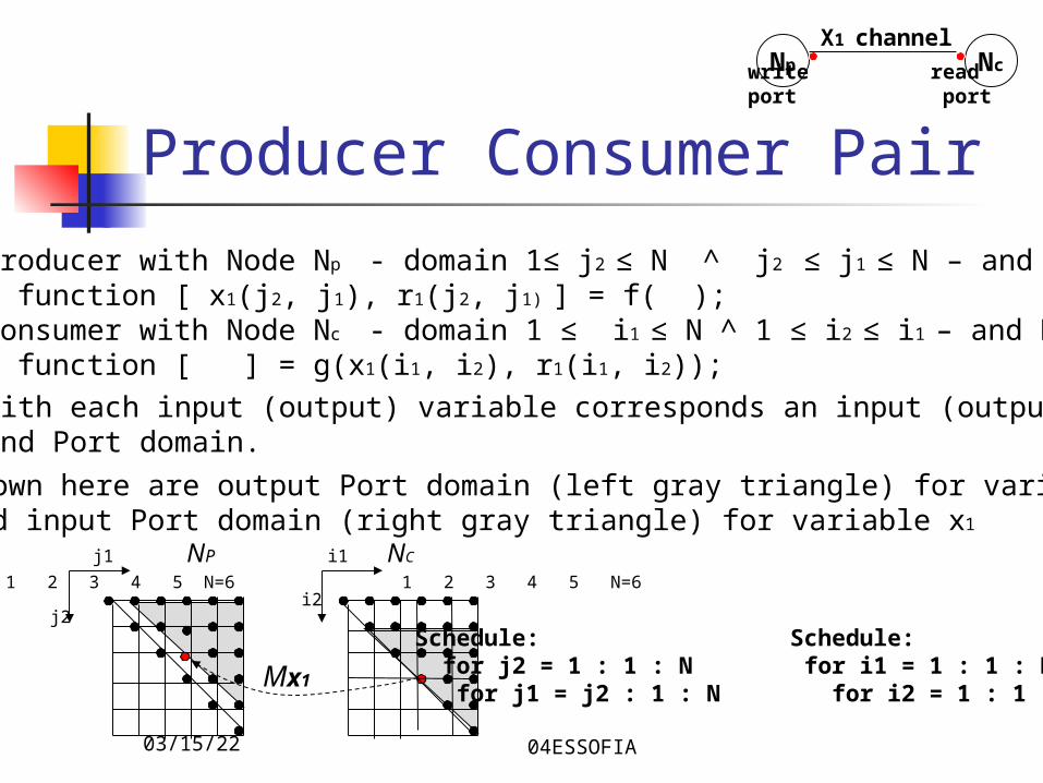
Producer with Node Np - domain 1≤ j2 ≤ N ^ j2 ≤ j1 ≤ N – and Node function [ x1(j2, j1), r1(j2, j1) ] = f( );Consumer with Node Nc - domain 1 ≤ i1 ≤ N ^ 1 ≤ i2 ≤ i1 – and Node function [ ] = g(x1(i1, i2), r1(i1, i2));
With each input (output) variable corresponds an input (output) Portand Port domain.
Shown here are output Port domain (left gray triangle) for variable x1
and input Port domain (right gray triangle) for variable x1
Np Nc
X1 channel
write readport port
NP NC
j2
1 2 3 4 5 N=6 1 2 3 4 5 N=6
j1 i1
i2
Mx1
Schedule: Schedule: for j2 = 1 : 1 : N for i1 = 1 : 1 : N for j1 = j2 : 1 : N for i2 = 1 : 1 : i1
04/18/23 04ESSOFIA
Producer Consumer Pair (2)
j2 = Mx1( i1 ) is the (dependency) affine mapping function,j1 i2
NP NC
j2
1 2 3 4 5 N=6 1 2 3 4 5 N=6
j1 i1
i2
Mx1
Schedule: Schedule: for j2 = 1 : 1 : N for i1 = 1 : 1 : N for j1 = j2 : 1 : N for i2 = 1 : 1 : i1
Here: j2 = 0 1 i1 + -1 j1 1 0 i2 0
right (4,4) → left (3,4)
Consumer takes from producer ‘function’ But – of course – producer tokens are sent to consumer
Np Nc
X1 channel
write readport port
04/18/23 04ESSOFIA
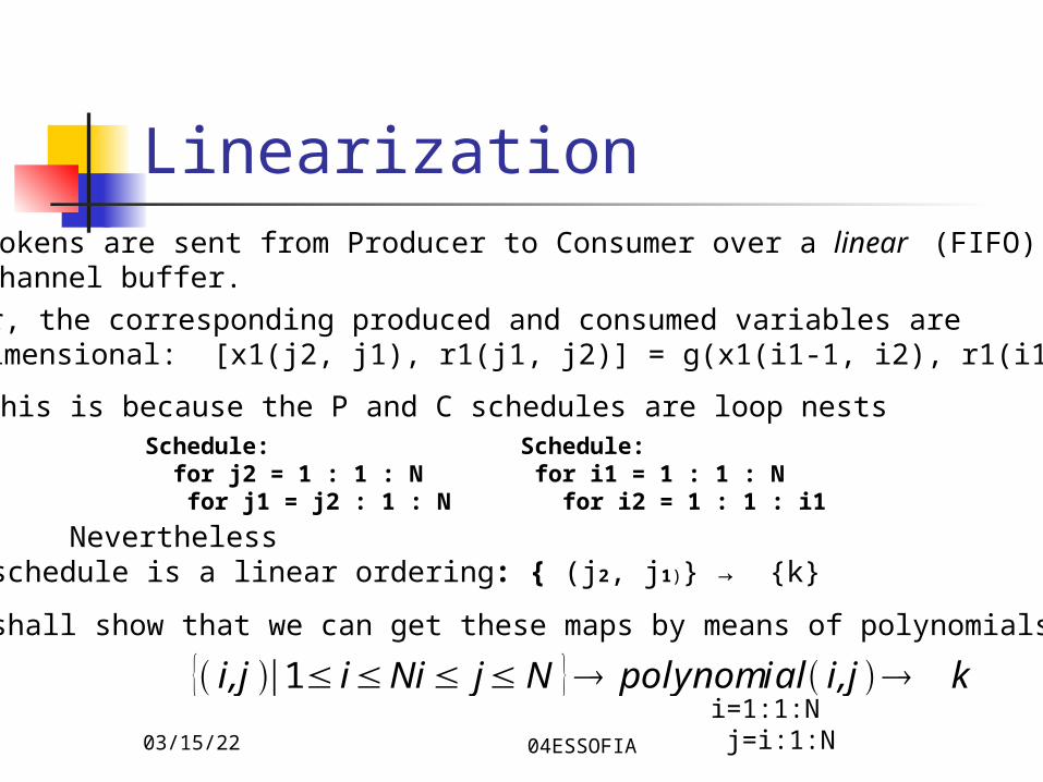
Linearization
{ i,j ∣1≤ i≤Ni≤ j≤ N } polynomial i,j ki=1:1:N j=i:1:N
Tokens are sent from Producer to Consumer over a linear (FIFO)Channel buffer.
However, the corresponding produced and consumed variables are multidimensional: [x1(j2, j1), r1(j1, j2)] = g(x1(i1-1, i2), r1(i1, i2));
This is because the P and C schedules are loop nestsSchedule: Schedule: for j2 = 1 : 1 : N for i1 = 1 : 1 : N for j1 = j2 : 1 : N for i2 = 1 : 1 : i1
a schedule is a linear ordering: { (j2, j1)} → {k}Nevertheless
I shall show that we can get these maps by means of polynomials:
04/18/23 04ESSOFIA
Linearization (2)
For the given domain {(i,j) | 1 ≤ i ≤ N ^ i ≤ j ≤ N}, and the givenlexicographic order: for i = 1 : 1 : N, for j = i : 1 : N, thereexists a (pseudo) polynomial E(i,j) such that, if (i’,j’ ) is the lexicographic k-th vector, then E(i’,j’ ) = k.
Pseudo polynomial to be defined on next slide.
Because the polynomial E(i,j) represents a ranking of vectors, we call itthe ranking polynomial.
Underlying theory is polynomial counting of integral points in polytopes.
i=1:1:N j=i:1:N
04/18/23 04ESSOFIA
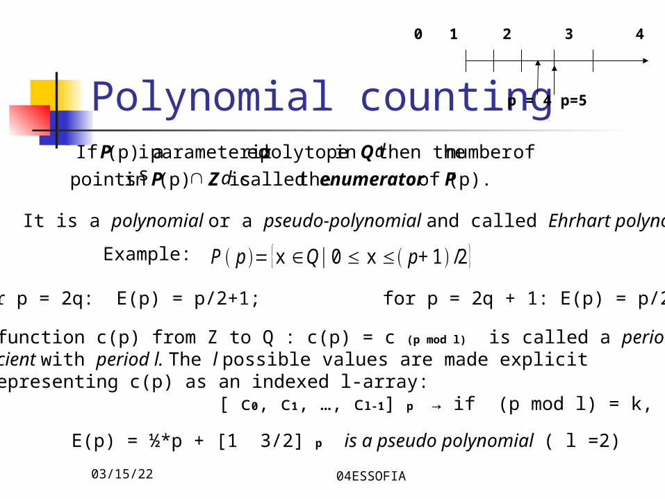
Polynomial counting
It is a polynomial or a pseudo-polynomial and called Ehrhart polynomial E(p).
Example: P p = {x ∈Q∣ 0 ≤ x ≤ p+ 1 /2 }
for p = 2q: E(p) = p/2+1; for p = 2q + 1: E(p) = p/2 + 3/2
The function c(p) from Z to Q : c(p) = c (p mod l) is called a periodiccoefficient with period l. The l possible values are made explicitby representing c(p) as an indexed l-array: [ c0, c1, …, cl-1] p → if (p mod l) = k, then ck
(p). of thecalled is (p)in points
ofnumber then thein polytope edparameteriz a is (p) If
PenumeratorZP
QP
d
d
E(p) = ½*p + [1 3/2] p is a pseudo polynomial ( l =2)
0 1 2 3 4
p = 4 p=5
04/18/23 04ESSOFIA
Theorem
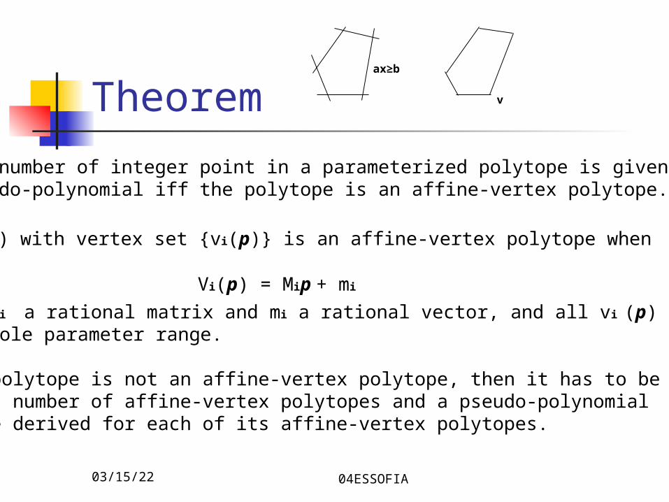
The number of integer point in a parameterized polytope is given as a pseudo-polynomial iff the polytope is an affine-vertex polytope.
P(p) with vertex set {vi(p)} is an affine-vertex polytope when
Vi(p) = Mip + mi
With Mi a rational matrix and mi a rational vector, and all vi (p) valid forthe whole parameter range.
If a polytope is not an affine-vertex polytope, then it has to be partitionedinto a number of affine-vertex polytopes and a pseudo-polynomialcan be derived for each of its affine-vertex polytopes.
ax≥b
v
04/18/23 04ESSOFIA
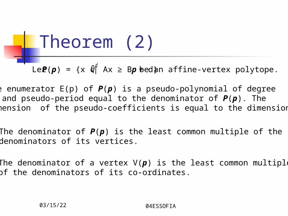
Theorem (2)
The enumerator E(p) of P(p) is a pseudo-polynomial of degreed and pseudo-period equal to the denominator of P(p). Thedimension of the pseudo-coefficients is equal to the dimension of p.
The denominator of P(p) is the least common multiple of thedenominators of its vertices.
The denominator of a vertex V(p) is the least common multipleof the denominators of its co-ordinates.
P(p) = {x є Qd| Ax ≥ Bp + d}Let be an affine-vertex polytope.
04/18/23 04ESSOFIA
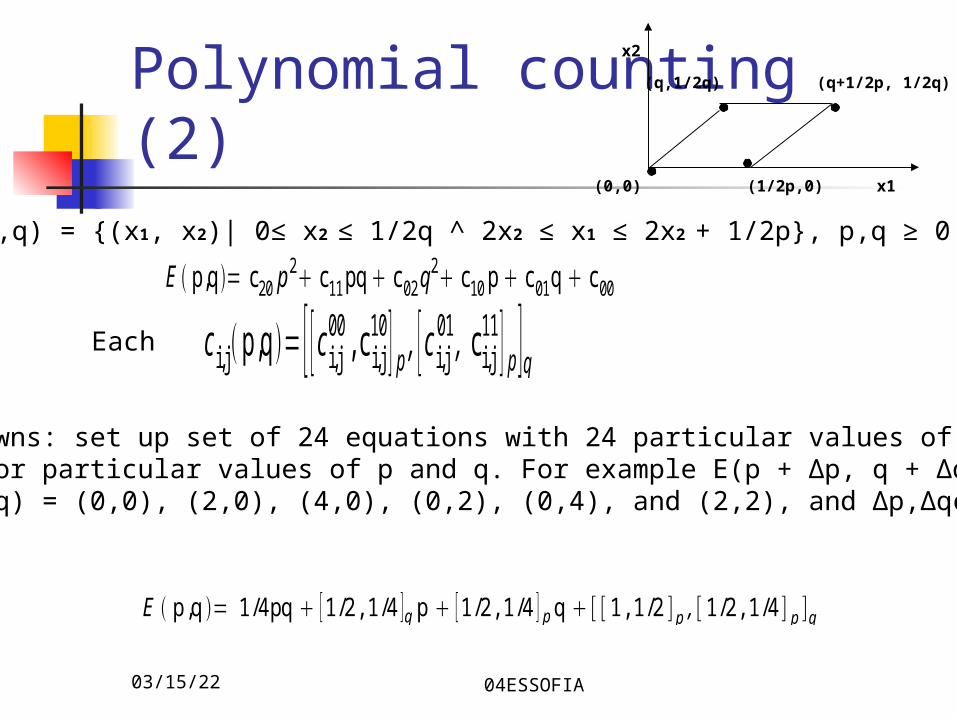
Polynomial counting (2)P(p,q) = {(x1, x2)| 0≤ x2 ≤ 1/2q ^ 2x2 ≤ x1 ≤ 2x2 + 1/2p}, p,q ≥ 0
E p,q = c20 p 2 c11 pq c 02 q2 c10 p c 01q c 00
c i,j p,q = [ [c i,j00 , c i,j
10 ] p , [ c i,j01 , c i,j
11 ] p ]qEach
24 unknowns: set up set of 24 equations with 24 particular values ofE(p,q) for particular values of p and q. For example E(p + Δp, q + Δq)with (p,q) = (0,0), (2,0), (4,0), (0,2), (0,4), and (2,2), and Δp,Δqє{0,1}.
E p ,q = 1 /4pq [1/2 , 1 /4 ]q p [1/2 , 1 /4 ] p q [ [ 1 , 1 /2 ] p , [ 1/2 , 1 /4 ] p ]q
(0,0) (1/2p,0)
(q,1/2q) (q+1/2p, 1/2q)
x1
x2
04/18/23 04ESSOFIA
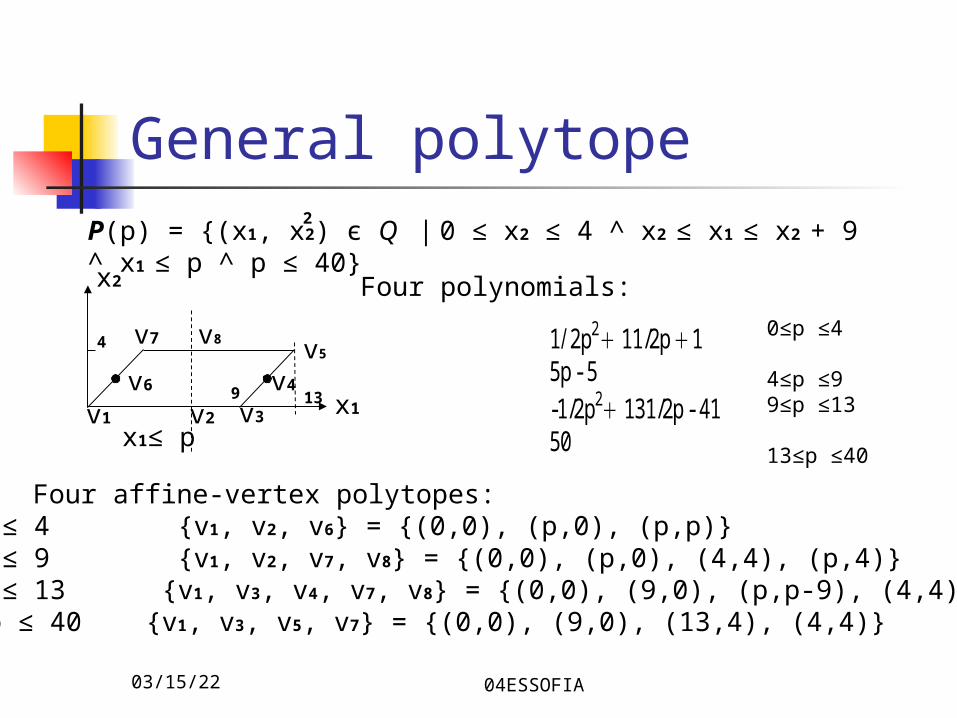
General polytopeP(p) = {(x1, x2) є Q | 0 ≤ x2 ≤ 4 ^ x2 ≤ x1 ≤ x2 + 9 ^ x1 ≤ p ^ p ≤ 40}
2
4
9 13 x1
x2
v1 v2 v3
v4
v5
v6
v7 v8
x1≤ p
Four affine-vertex polytopes:0 ≤ p ≤ 4 {v1, v2, v6} = {(0,0), (p,0), (p,p)}4 ≤ p ≤ 9 {v1, v2, v7, v8} = {(0,0), (p,0), (4,4), (p,4)}9 ≤ p ≤ 13 {v1, v3, v4, v7, v8} = {(0,0), (9,0), (p,p-9), (4,4), (p,4)}13 ≤ p ≤ 40 {v1, v3, v5, v7} = {(0,0), (9,0), (13,4), (4,4)}
Four polynomials:
1 /2p2 11/2p 15p - 5-1/2p2 131/2p - 4150
0≤p ≤4
4≤p ≤99≤p ≤13
13≤p ≤40
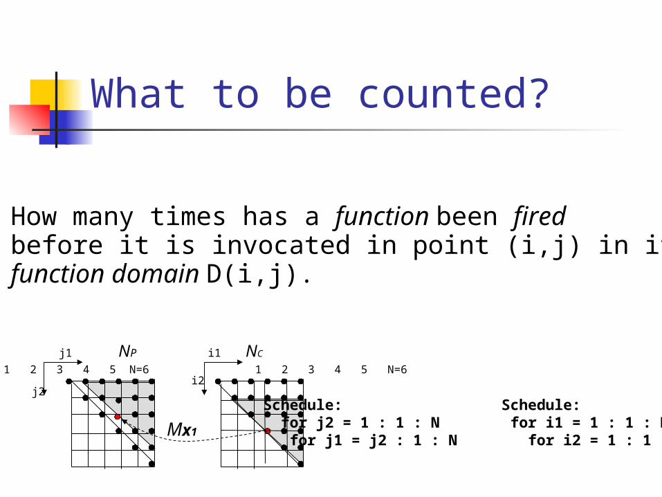
What to be counted?
How many times has a function been firedbefore it is invocated in point (i,j) in itsfunction domain D(i,j).
NP NC
j2
1 2 3 4 5 N=6 1 2 3 4 5 N=6
j1 i1
i2
Mx1
Schedule: Schedule: for j2 = 1 : 1 : N for i1 = 1 : 1 : N for j1 = j2 : 1 : N for i2 = 1 : 1 : i1
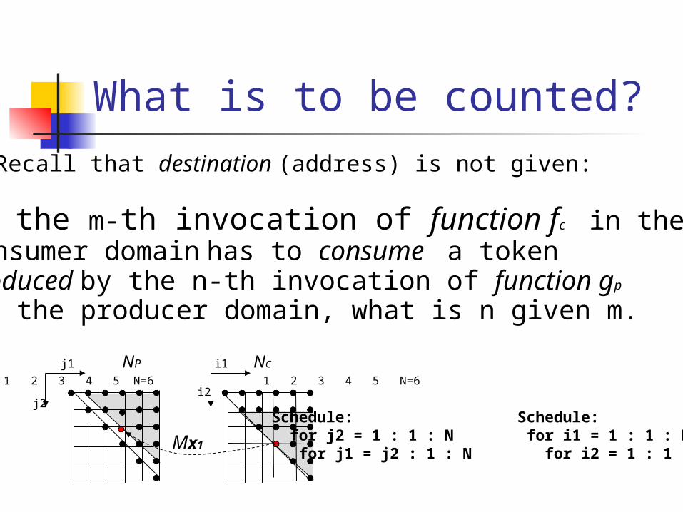
What is to be counted?
If the m-th invocation of function fc in theconsumer domain has to consume a token produced by the n-th invocation of function gp
in the producer domain, what is n given m.
NP NC
j2
1 2 3 4 5 N=6 1 2 3 4 5 N=6
j1 i1
i2
Mx1
Schedule: Schedule: for j2 = 1 : 1 : N for i1 = 1 : 1 : N for j1 = j2 : 1 : N for i2 = 1 : 1 : i1
Recall that destination (address) is not given:
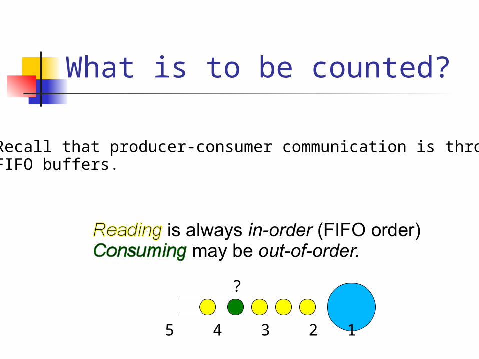
What is to be counted?
Recall that producer-consumer communication is throughFIFO buffers.
5 4 3 2 1
?
04/18/23 04ESSOFIA
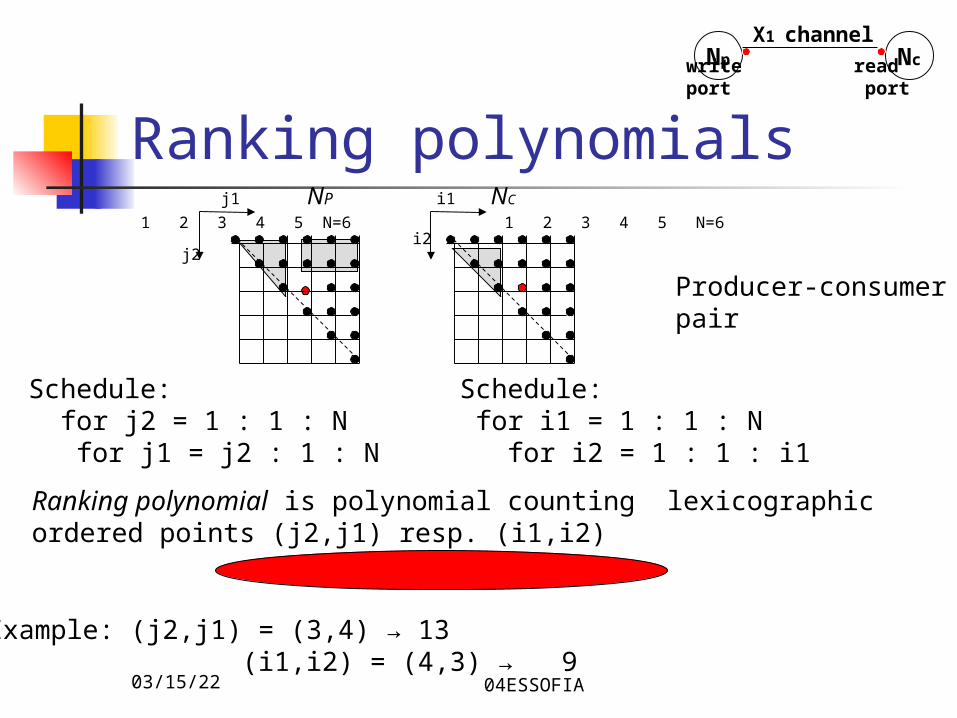
Ranking polynomials
Ranking polynomial is polynomial counting lexicographic ordered points (j2,j1) resp. (i1,i2)
Example: (j2,j1) = (3,4) → 13 (i1,i2) = (4,3) → 9
j2
NP NC
1 2 3 4 5 N=6 1 2 3 4 5 N=6
j1 i1
i2
Schedule: Schedule: for j2 = 1 : 1 : N for i1 = 1 : 1 : N for j1 = j2 : 1 : N for i2 = 1 : 1 : i1
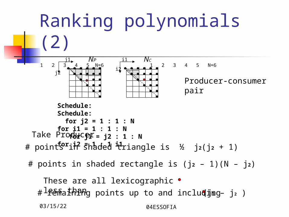
Producer-consumerpair
Np Nc
X1 channel
write readport port
04/18/23 04ESSOFIA
Ranking polynomials (2)
Take Producer
# points in shaded triangle is ½ j2(j2 + 1)
# points in shaded rectangle is (j2 – 1)(N – j2)
These are all lexicographic less than # remaining points up to and including (j1 – j2 )
j2
NP NC1 2 3 4 5 N=6 1 2 3 4 5 N=6
j1 i1
i2
Schedule: Schedule: for j2 = 1 : 1 : N for i1 = 1 : 1 : N for j1 = j2 : 1 : N for i2 = 1 : 1 i1
Producer-consumerpair
04/18/23 04ESSOFIA
production and consumption polynomials
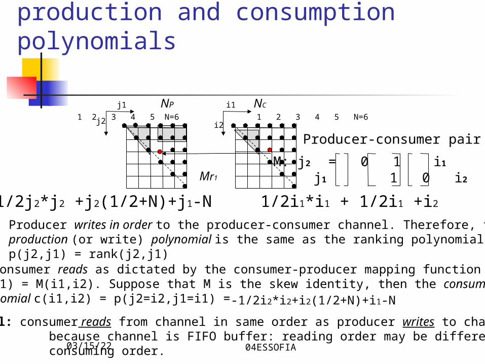
The consumer reads as dictated by the consumer-producer mapping function(j2,j1) = M(i1,i2). Suppose that M is the skew identity, then the consumption polynomial c(i1,i2) = p(j2=i2,j1=i1) =
Producer writes in order to the producer-consumer channel. Therefore, theproduction (or write) polynomial is the same as the ranking polynomial p(j2,j1) = rank(j2,j1)
Recall: consumer reads from channel in same order as producer writes to channel because channel is FIFO buffer: reading order may be different from consuming order.
NP NC
1 2 3 4 5 N=6 1 2 3 4 5 N=6
j1
j2
i1
i2
Mr1
Producer-consumer pair
M: j2 = 0 1 i1 j1 1 0 i2
-1/2j2*j2 +j2(1/2+N)+j1-N 1/2i1*i1 + 1/2i1 +i2
-1/2i2*i2+i2(1/2+N)+i1-N
04/18/23 04ESSOFIA
production and consumption polynomials(2)
NP NC
1 2 3 4 5 N=6 1 2 3 4 5 N=6
j1
j2
i1
i2
Mr1
−1 / 2j22N+ 1 / 2 j 2+j 1 -N 1 / 2i1
2−1 / 2i1+i 2
Producer-consumer pair
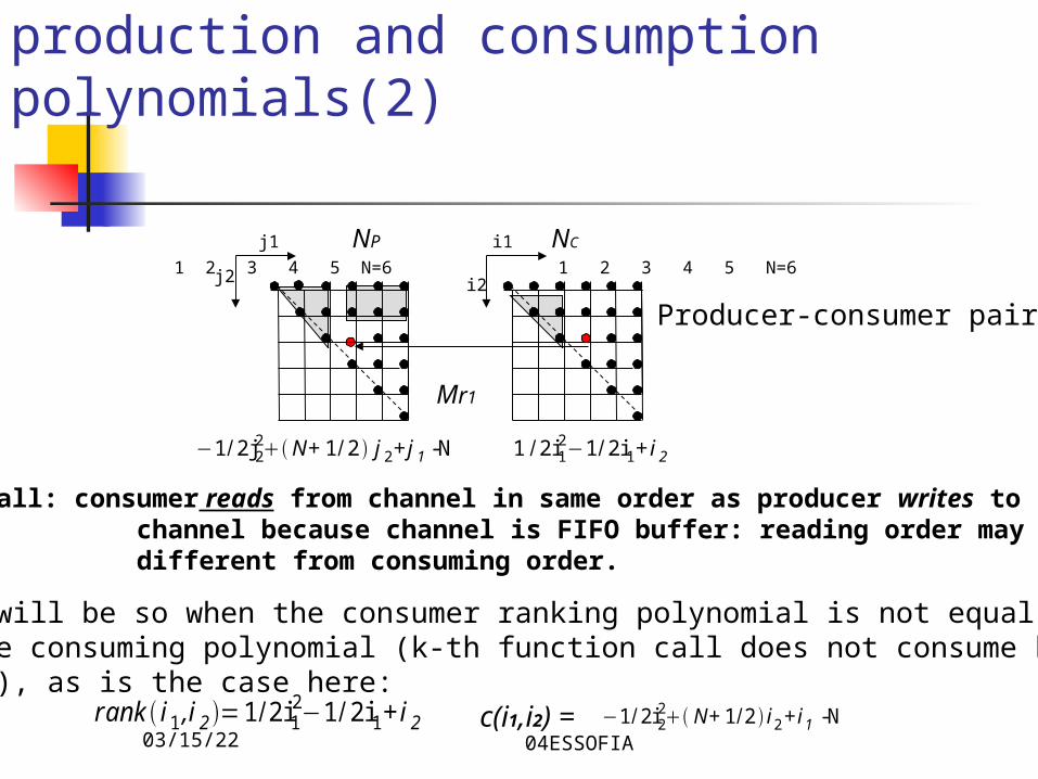
Recall: consumer reads from channel in same order as producer writes to channel because channel is FIFO buffer: reading order may be different from consuming order.
This will be so when the consumer ranking polynomial is not equalto the consuming polynomial (k-th function call does not consume k-th senttoken), as is the case here:
rank i1 ,i 2 =1 /2i12−1 / 2i1+i 2 c(i1,i2) = −1 / 2i2
2 N+1 /2 i2 +i1 -N
04/18/23 04ESSOFIA
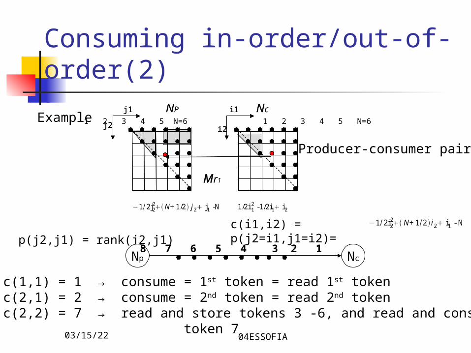
Consuming in-order/out-of-order
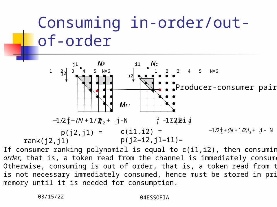
If consumer ranking polynomial is equal to c(i1,i2), then consuming is inorder, that is, a token read from the channel is immediately consumed.Otherwise, consuming is out of order, that is, a token read from the channelis not necessary immediately consumed, hence must be stored in privatememory until it is needed for consumption.
NP NCNP NC
1 2 3 4 5 N=6 1 2 3 4 5 N=6
j1
j2
i1
i2
Mr1
€
−1/2j22 +(N +1/2)j2 + j1 - N 1/2i1
2 -1/2i1 + i2
€
−1/2i22 +(N +1/2)i2 + i1 - N
j1
j2
i1
i2
M
p(j2,j1) = rank(j2,j1)
c(i1,i2) = p(j2=i2,j1=i1)=
Producer-consumer pair
04/18/23 04ESSOFIA
Consuming in-order/out-of-order(2)
ExampleNP NCNP NC
1 2 3 4 5 N=6 1 2 3 4 5 N=6
j1
j2
i1
i2
Mr1
−1 / 2j22 N+ 1/2 j2 j1 -N 1/2i 1
2 -1/2i1 i2
−1 / 2i22 N+ 1 /2 i2 i1 - N
j1
j2
i1
i2
M
p(j2,j1) = rank(j2,j1)
c(i1,i2) = p(j2=i1,j1=i2)=
Producer-consumer pair
Np Nc 8 7 6 5 4 3 2 1
c(1,1) = 1 → consume = 1st token = read 1st tokenc(2,1) = 2 → consume = 2nd token = read 2nd tokenc(2,2) = 7 → read and store tokens 3 -6, and read and consume token 7
04/18/23 04ESSOFIA
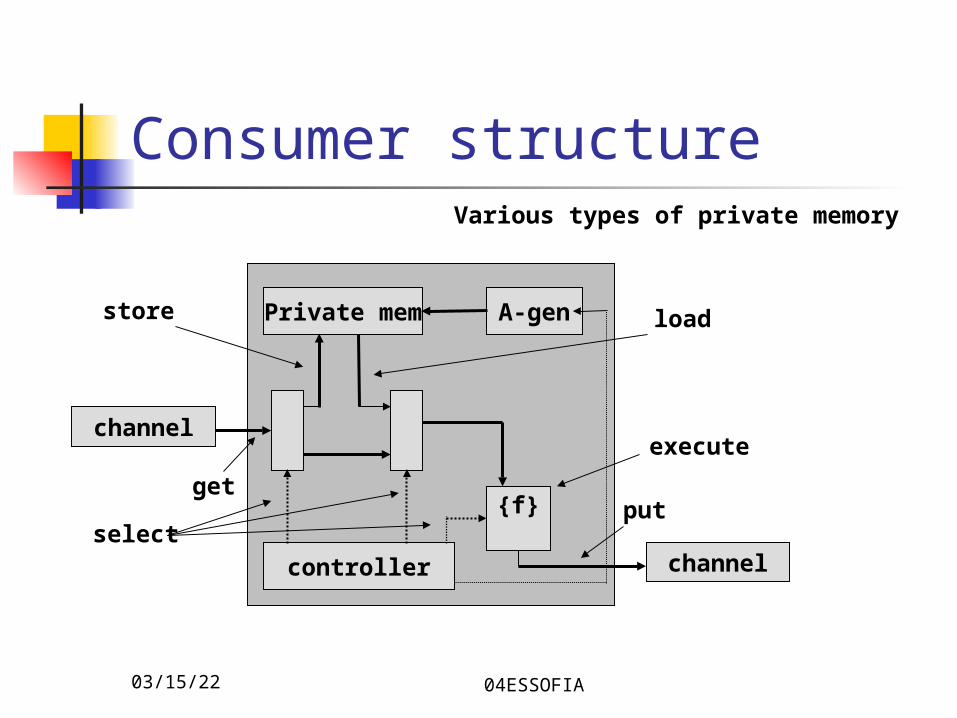
Consumer structure
Private mem A-gen
{f}
controller
channel
channel
store load
execute
getput
select
Various types of private memory
04/18/23 04ESSOFIA
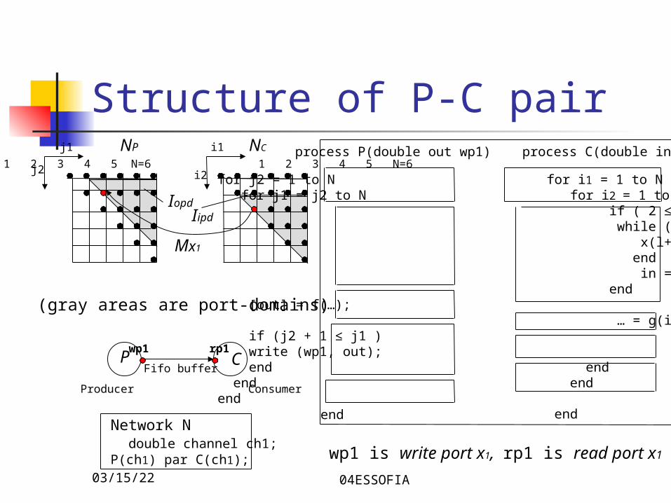
Structure of P-C pair
(gray areas are port-domains)
NP NC
1 2 3 4 5 N=6 1 2 3 4 5 N=6
j1
j2
i1
i2
Mx1
Iopd Iipd
process P(double out wp1) process C(double in rp1)
for j2 = 1 to N for i1 = 1 to N for j1 = j2 to N for i2 = 1 to i1 if ( 2 ≤ i2 ) while ( l < c(i1,i2) x(l++) = read(rp1); end in = x(c(i1,i2)); end [out] = f(…); … = g(in); if (j2 + 1 ≤ j1 ) write (wp1, out); end end end endend endend
wp1 is write port x1, rp1 is read port x1
P CFifo buffer
Producer Consumer
Network N double channel ch1;P(ch1) par C(ch1);
wp1 rp1
04/18/23 04ESSOFIA
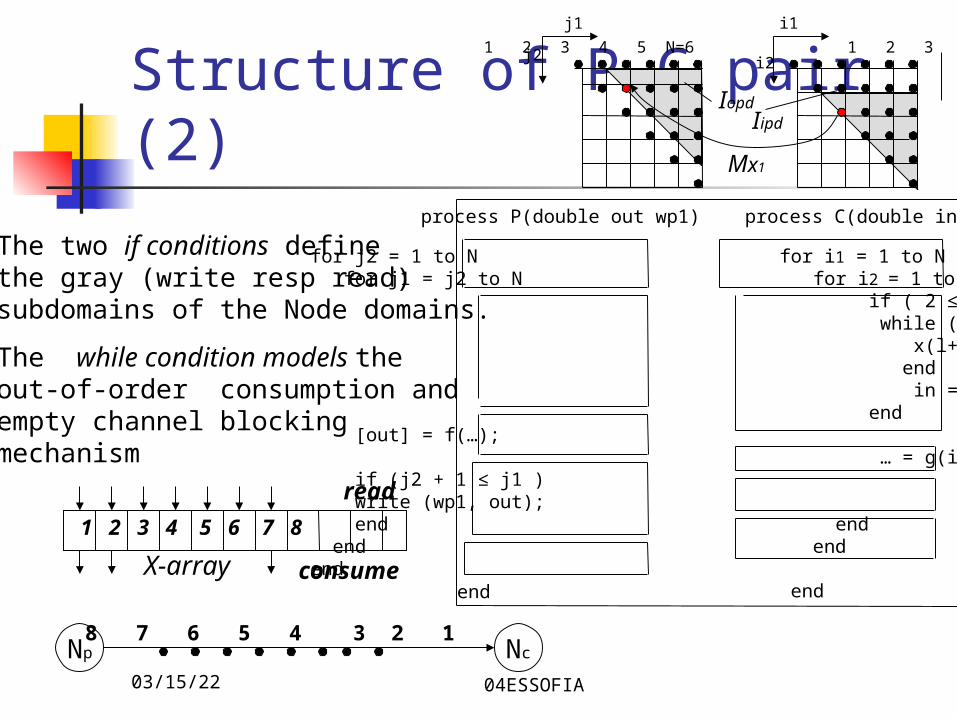
Structure of P-C pair (2)
The two if conditions definethe gray (write resp read)subdomains of the Node domains.
The while condition models theout-of-order consumption andempty channel blocking mechanism
Np Nc 8 7 6 5 4 3 2 1
X-array
1 2 3 4 5 6 7 8
read
consume
process P(double out wp1) process C(double in rp1)
for j2 = 1 to N for i1 = 1 to N for j1 = j2 to N for i2 = 1 to i1 if ( 2 ≤ i2 ) while ( l <= c(i1,i2) x(l++) = read(rp1); end in = x(c(i1,i2)); end [out] = f(…); … = g(in); if (j2 + 1 ≤ j1 ) write (wp1, out); end end end endend endend
1 2 3 4 5 N=6 1 2 3 4 5 N=6
j1
j2
i1
i2
Mx1
Iopd Iipd
04/18/23 04ESSOFIA
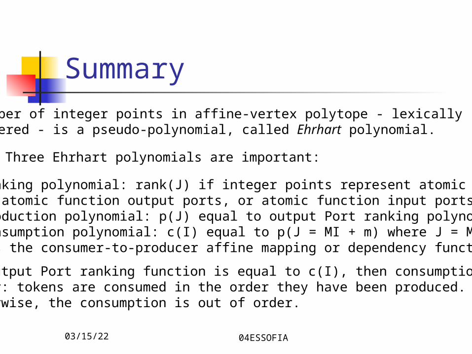
SummaryNumber of integer points in affine-vertex polytope - lexicallyordered - is a pseudo-polynomial, called Ehrhart polynomial.
Three Ehrhart polynomials are important:
• ranking polynomial: rank(J) if integer points represent atomic functions, atomic function output ports, or atomic function input ports.• production polynomial: p(J) equal to output Port ranking polynomial• consumption polynomial: c(I) equal to p(J = MI + m) where J = MI+m is the consumer-to-producer affine mapping or dependency function.
If output Port ranking function is equal to c(I), then consumption is inorder: tokens are consumed in the order they have been produced.Otherwise, the consumption is out of order.
04/18/23 04ESSOFIA
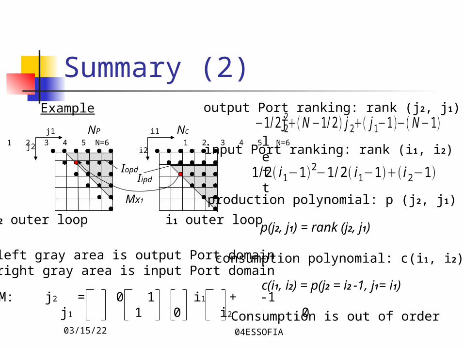
Summary (2)Example
NP NC
1 2 3 4 5 N=6 1 2 3 4 5 N=6
j1
j2
i1
i2
Mx1
Iopd Iipd
j2 outer loop i1 outer loop
left gray area is output Port domainright gray area is input Port domain
M: j2 = 0 1 i1 + -1 j1 1 0 i2 0
−1 / 2j22N −1 / 2 j 2 j1−1 − N −1
left
output Port ranking: rank (j2, j1)
input Port ranking: rank (i1, i2)
1 / 2 i1−1 2−1 / 2 i1−1 i2−1
production polynomial: p (j2, j1)
p(j2, j1) = rank (j2, j1)
consumption polynomial: c(i1, i2)
c(i1, i2) = p(j2 = i2 -1, j1= i1)
Consumption is out of order
04/18/23 04ESSOFIA
Multiplicity
If p consecutive tokens sent by the producer have equalvalue, then this token is sent only once and said to havemultiplicity p.
The consumer, then, stores that token in private memory andconsumes it p times, after which the storage location isreleased.
There are thus 4 cases: in-order without multiplicity (IOM-) in-order with multiplicity (IOM+) out-of-order without multiplicity (OOM-) out-of-order with multiplicity (OOM+)
04/18/23 04ESSOFIA
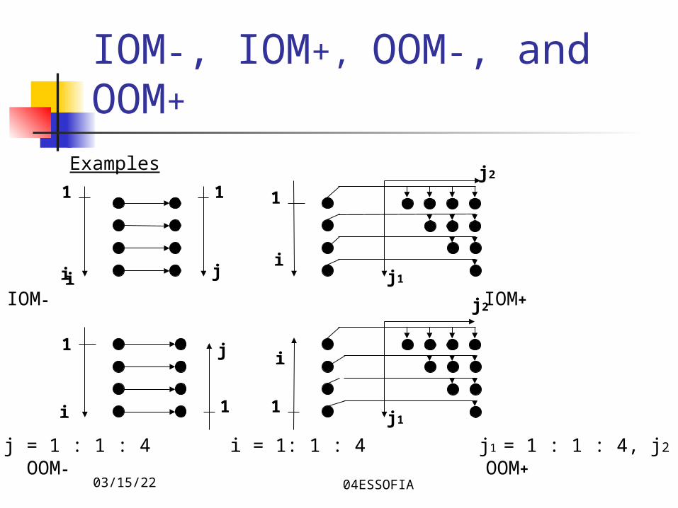
IOM-, IOM+, OOM-, and OOM+
Examples j2
i ji
i
j
1 1
1
1
i = 1 : 1 : 4 j = 1 : 1 : 4 i = 1: 1 : 4 j1 = 1 : 1 : 4, j2 = j1 : 1 : 4
i
i
j1
j1
j2
1
1
IOM- IOM+
OOM- OOM+
04/18/23 04ESSOFIA
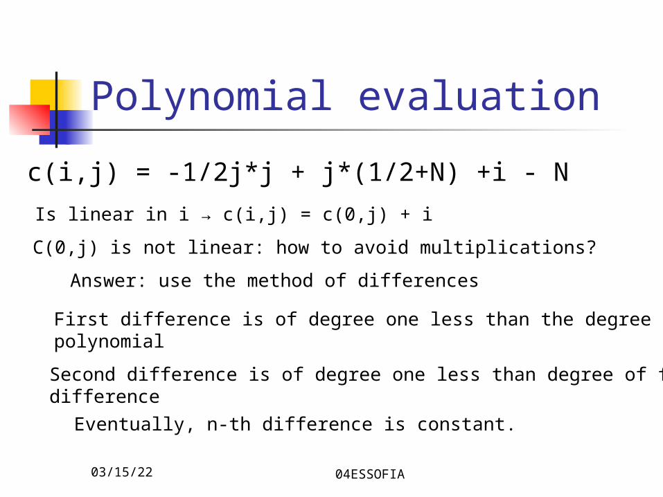
Polynomial evaluation
Is linear in i → c(i,j) = c(0,j) + i
C(0,j) is not linear: how to avoid multiplications?
Answer: use the method of differences
First difference is of degree one less than the degree of the polynomial
Second difference is of degree one less than degree of firstdifference
Eventually, n-th difference is constant.
c(i,j) = -1/2j*j + j*(1/2+N) +i - N
04/18/23 04ESSOFIA
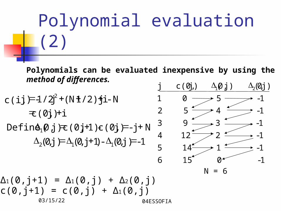
Polynomial evaluation (2)
Polynomials can be evaluated inexpensive by using themethod of differences.
1- j),0( - )1j,0( j),0(
N j- j)c(0, - 1)jc(0, j)0,( Define
i j)c(0,
N- i 1/2)jN(j 1/2- j)c(i,
112
1
2
1- 0 15 6
1- 1 14 5
1- 2 12 4
1- 3 9 3
1- 4 5 2
1- 5 0 1
j),0( j)0,( j)c(0, j 21
N = 6Δ1(0,j+1) = Δ1(0,j) + Δ2(0,j)c(0,j+1) = c(0,j) + Δ1(0,j)
04/18/23 04ESSOFIA
register
adder
register
adder
load N if j=1
Load 0 if j=1
adder
i
-1
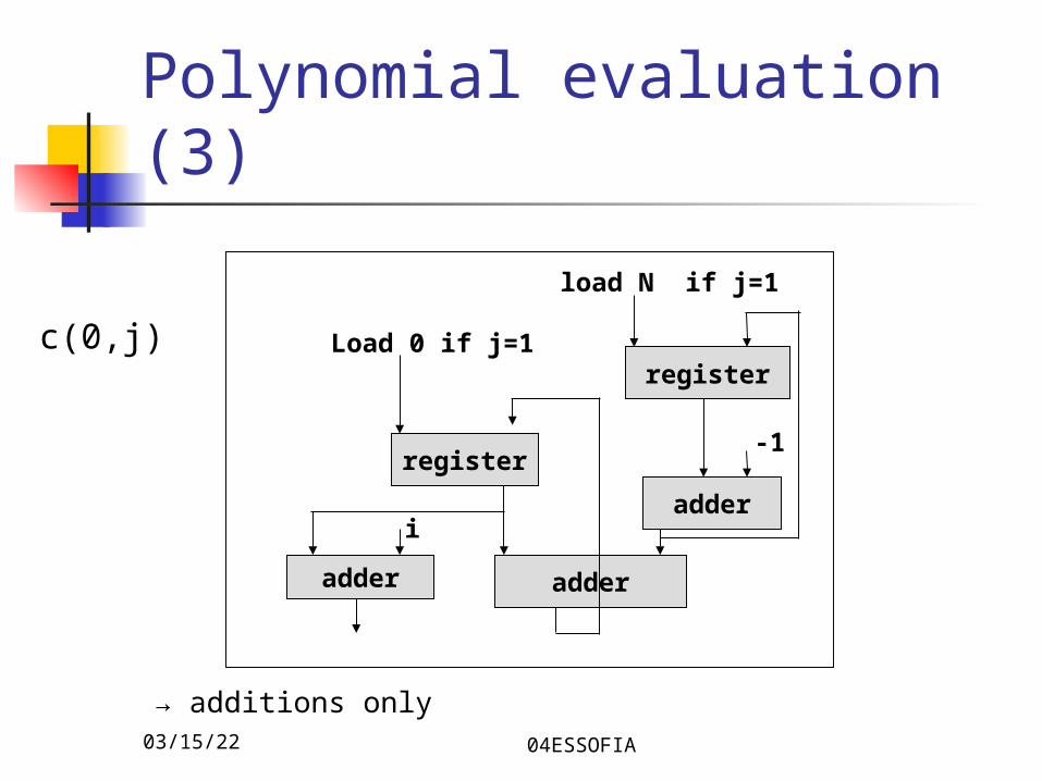
Polynomial evaluation (3)
→ additions only
c(0,j)
04/18/23 04ESSOFIA
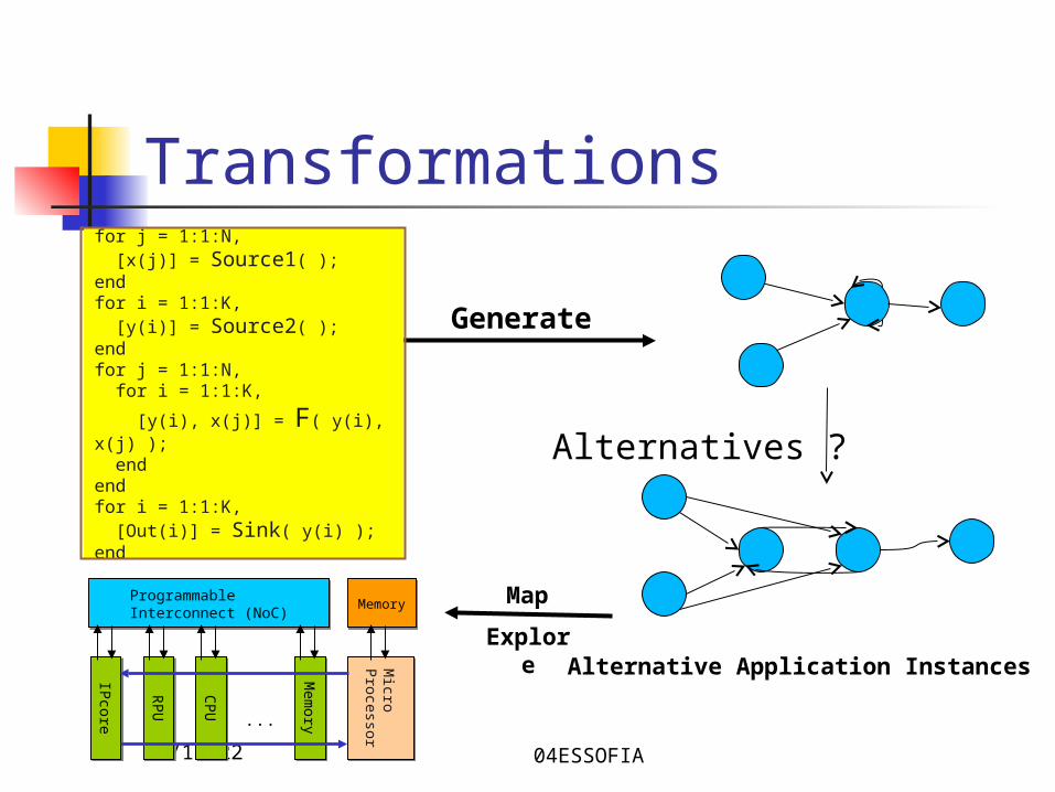
Transformations
Programmable Interconnect (NoC)Programmable Interconnect (NoC)
IPcore
IPcore
RP
UR
PU
Mem
oryM
emory
CP
UC
PU
Micro
Processor
Micro
Processor
MemoryMemory
...
Alternative Application Instances
Generate
Map
Explore
for j = 1:1:N, [x(j)] = Source1( ); endfor i = 1:1:K, [y(i)] = Source2( ); endfor j = 1:1:N, for i = 1:1:K,
[y(i), x(j)] = F( y(i), x(j) ); endendfor i = 1:1:K, [Out(i)] = Sink( y(i) ); end
Alternatives ?
Alternatives
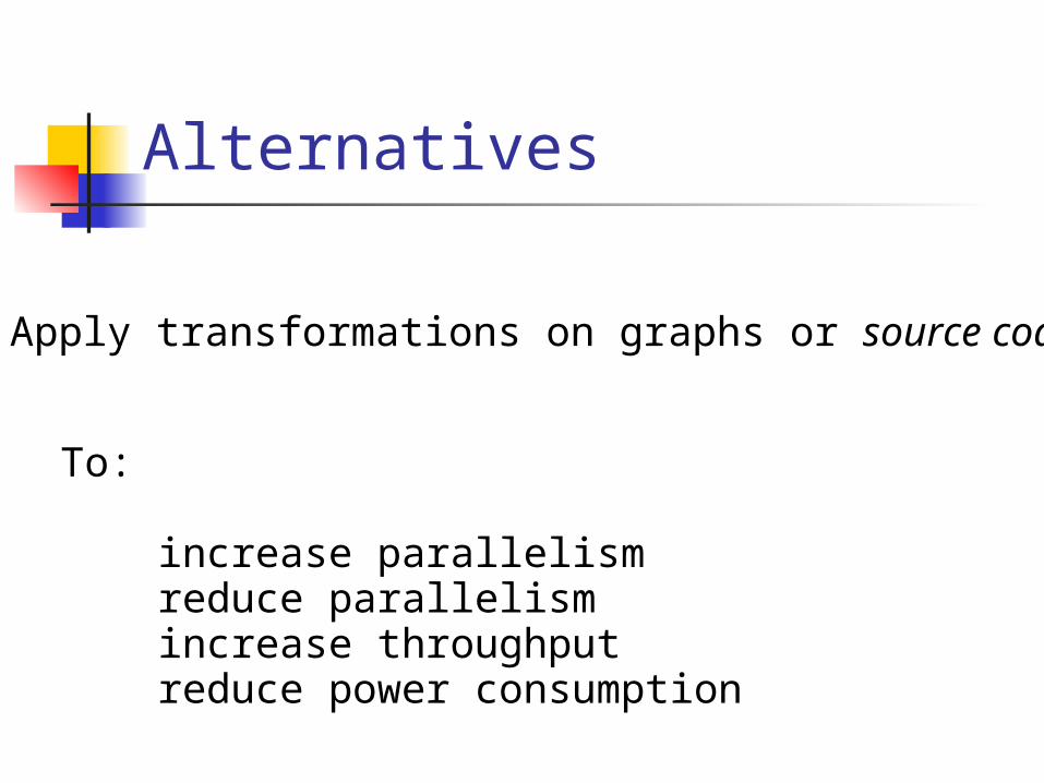
Apply transformations on graphs or source code.
To:
increase parallelism reduce parallelism increase throughput reduce power consumption
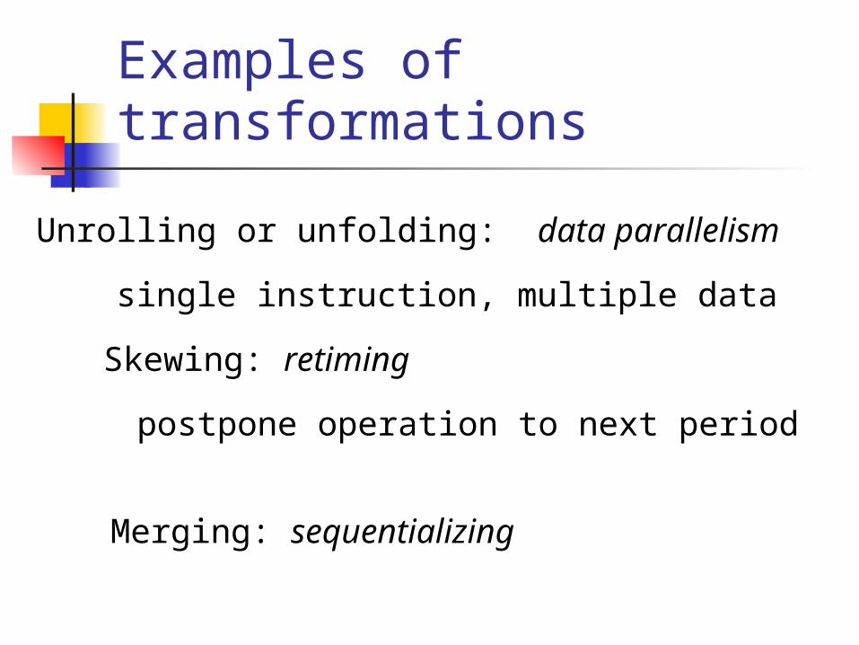
Examples of transformations
Unrolling or unfolding: data parallelism
single instruction, multiple data
Skewing: retiming
postpone operation to next period
Merging: sequentializing
04/18/23 04ESSOFIA
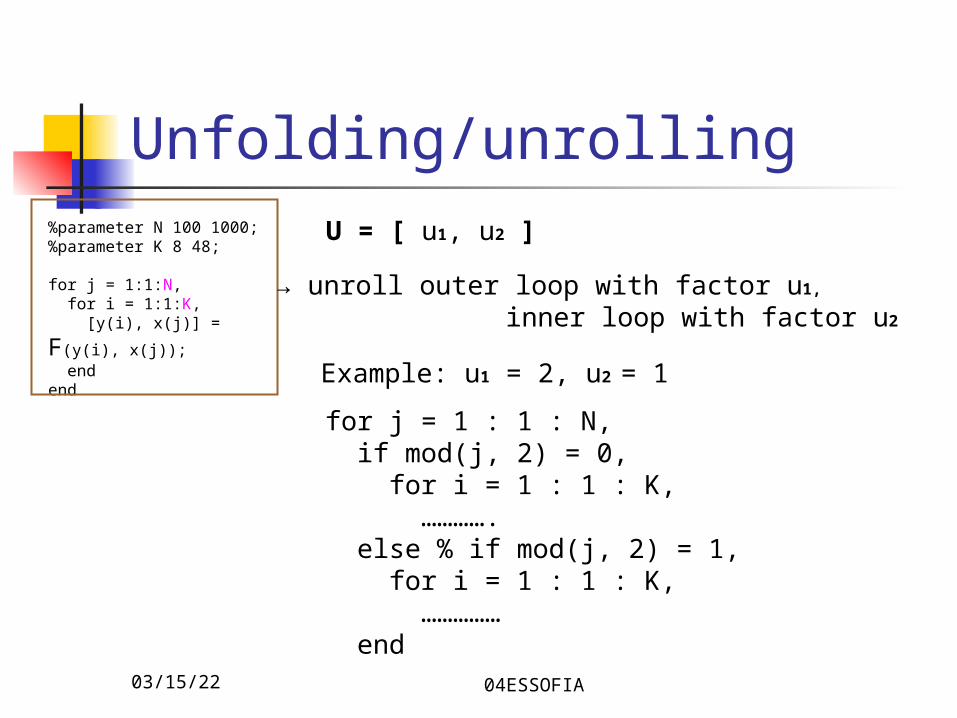
Unfolding/unrolling%parameter N 100 1000;%parameter K 8 48;
for j = 1:1:N, for i = 1:1:K,
[y(i), x(j)] = F(y(i), x(j)); endend
U = [ u1, u2 ]
→ unroll outer loop with factor u1,
inner loop with factor u2
Example: u1 = 2, u2 = 1
for j = 1 : 1 : N, if mod(j, 2) = 0, for i = 1 : 1 : K, …………. else % if mod(j, 2) = 1, for i = 1 : 1 : K, …………… end
04/18/23 04ESSOFIA
Unrolling/Unfolding (2)
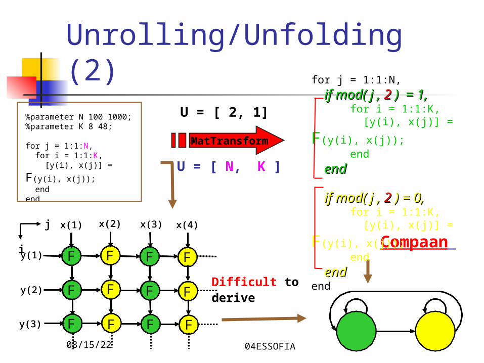
%parameter N 100 1000;%parameter K 8 48;
for j = 1:1:N, for i = 1:1:K,
[y(i), x(j)] = F(y(i), x(j)); endend
F F F F
F
F
F
F
F
F
F
F
x(1) x(2) x(3) x(4)
y(1)
y(2)
y(3)
j
iF F F F
F
F
F
F
F
F
F
F
x(1) x(2) x(3) x(4)
y(1)
y(2)
y(3)
j
i Compaan
U = [ N, K ]
Difficult to derive
for j = 1:1:N, if mod( j , if mod( j , 2 2 ) = 1,) = 1, for i = 1:1:K,
[y(i), x(j)] = F(y(i), x(j)); end endend
if mod( j , if mod( j , 2 2 ) = 0,) = 0, for i = 1:1:K,
[y(i), x(j)] = F(y(i), x(j)); end endendend
MatTransform
U = [ 2, 1]
04/18/23 04ESSOFIA
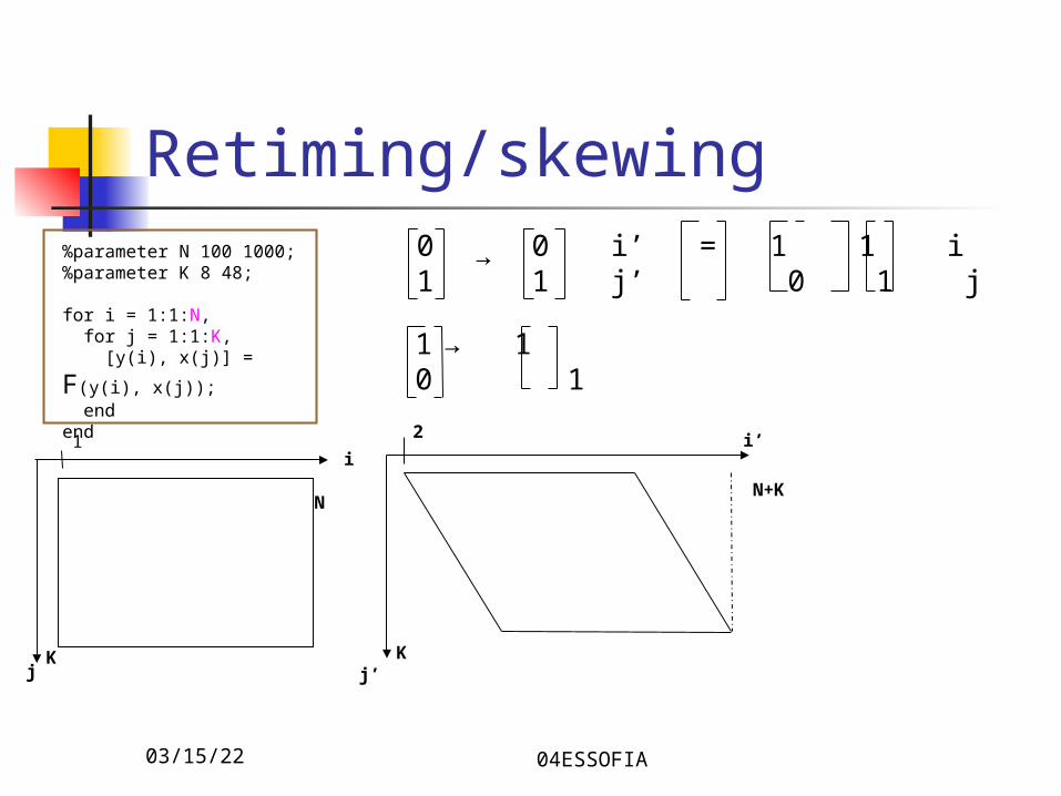
Retiming/skewing%parameter N 100 1000;%parameter K 8 48;
for i = 1:1:N, for j = 1:1:K,
[y(i), x(j)] = F(y(i), x(j)); endend
01
→ 01
10
→ 1 1
i’ = 1 1 i j’ 0 1 j
j’
N+K
K
2 i’i
j
N
K
1
Skewing
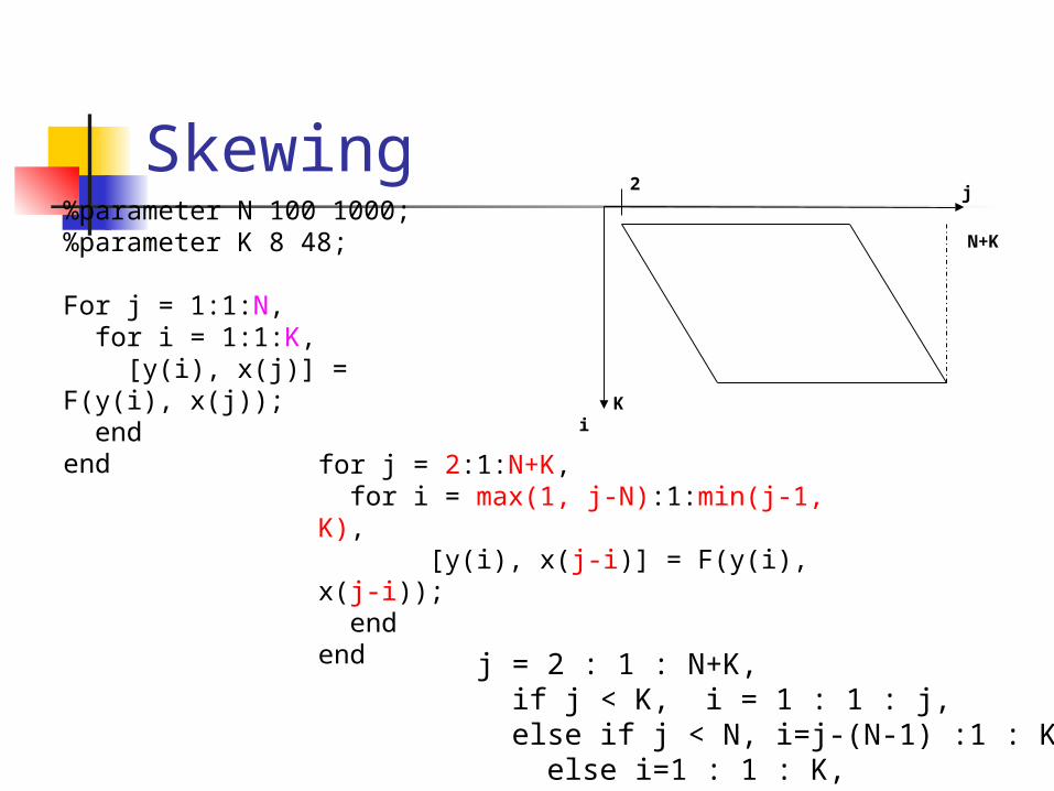
for j = 2:1:N+K, for i = max(1, j-N):1:min(j-1, K), [y(i), x(j-i)] = F(y(i), x(j-i)); endend
%parameter N 100 1000;%parameter K 8 48;
For j = 1:1:N, for i = 1:1:K, [y(i), x(j)] = F(y(i), x(j)); endend
j = 2 : 1 : N+K, if j < K, i = 1 : 1 : j, else if j < N, i=j-(N-1) :1 : K, else i=1 : 1 : K,
i
N+K
K
2 j
04/18/23 04ESSOFIA
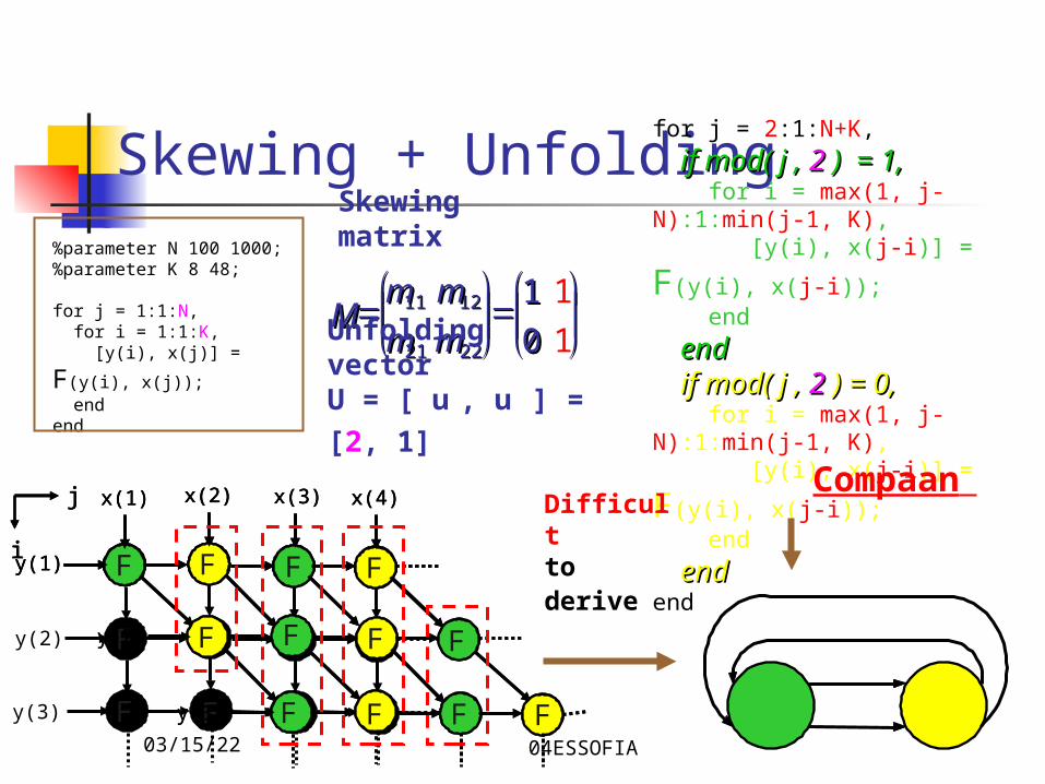
Skewing + UnfoldingSkewing matrix
100
111
22222121
12121111
mmmm
mmmmMM
F F F F
F
F
F
F
F
F
F
F
x(1) x(2) x(3) x(4)
y(1)
y(2)
y(3)
j
i
for j = 2:1:N+K, if mod( j , if mod( j , 22 ) = 1,) = 1, for i = max(1, j-N):1:min(j-1, K),
[y(i), x(j-i)] = F(y(i), x(j-i)); end endend if mod( j , if mod( j , 22 ) = 0,) = 0, for i = max(1, j-N):1:min(j-1, K),
[y(i), x(j-i)] = F(y(i), x(j-i)); end endendendF F F F
F
F
F
F
F
F
F
F
x(1) x(2) x(3) x(4)
y(1)
y(2)
y(3)
j
iF F F F
F
F
F
F
F
F
F
F
x(1) x(2) x(3) x(4)
y(1)
y(2)
y(3)
j
i
Unfolding vectorU = [ u
1, u
2 ] = [2, 1]
Compaan Difficult
to derive
%parameter N 100 1000;%parameter K 8 48;
for j = 1:1:N, for i = 1:1:K,
[y(i), x(j)] = F(y(i), x(j)); endend
04/18/23 04ESSOFIA
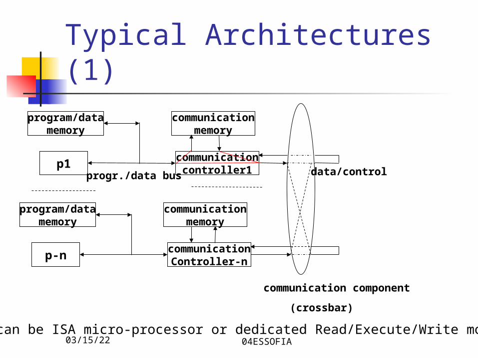
Typical Architectures (1)program/data
memory
p1communication
controller1
communicationmemory
program/datamemory
p-ncommunication
Controller-n
communicationmemory
progr./data bus data/control
(crossbar)
communication component
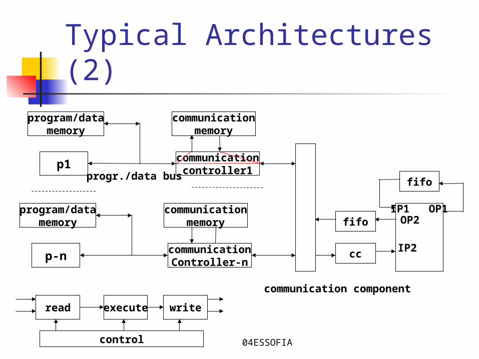
p-x can be ISA micro-processor or dedicated Read/Execute/Write module
04/18/23 04ESSOFIA
Typical Architectures (2)program/data
memory
p1communication
controller1
communicationmemory
program/datamemory
p-ncommunication
Controller-n
communicationmemory
progr./data bus
communication component
cc
fifo
fifo
IP1 OP1OP2
IP2
read writeexecute
control
04/18/23 04ESSOFIA
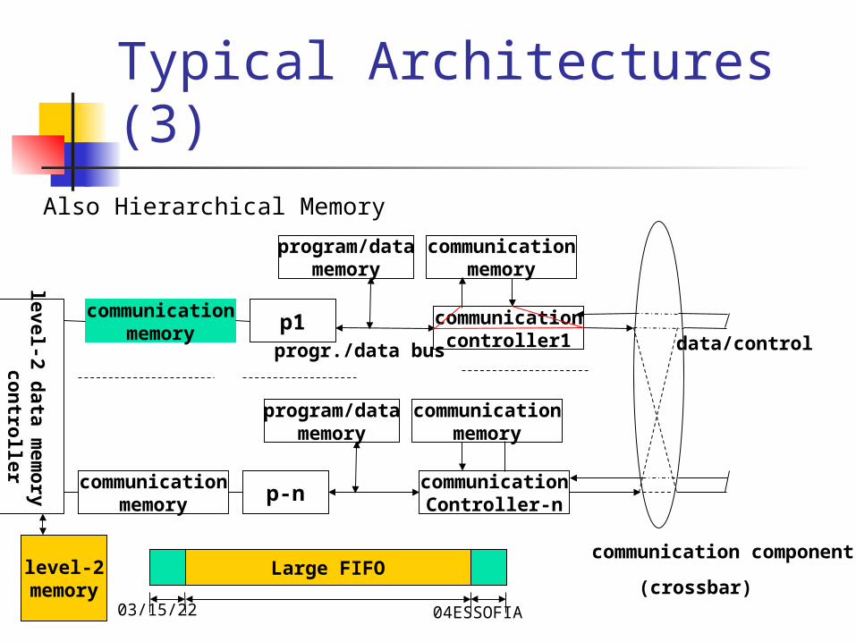
Typical Architectures (3)Also Hierarchical Memory
program/datamemory
p1 communicationcontroller1
communicationmemory
program/datamemory
p-ncommunication
Controller-n
communicationmemory
progr./data bus data/control
(crossbar)
communication component
communicationmemory
communicationmemory
level-2memory
level-2 data
mem
ory
con
troller
Large FIFO
04/18/23 04ESSOFIA
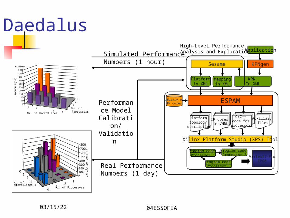
Daedalus
Library ofIP cores
Platformin XML
C/C++ code for
processors
IP cores in VHDL
Mappingin XML
Platform topology
description
Xilinx Platform Studio (XPS) Tool
VirtexII-ProFPGA
Application
Auxiliary files
Program code Processor 1
Program code Processor 2
Program code Processor 3
ESPAM
Sesame KPNgen
KPN In XML
High-Level Performance Analysis and Exploration Simulated Performance
Numbers (1 hour)
0 1 23
4
12
3
4
0
50
100
150
200
250
300
350
400
450
500
Cycle n
um
be
r
Millions
Nr. of MicroBlazes
Nr. of Processors
Real Performance Numbers (1 day)0
12
34
43
21
0100200300400500600700800
Million of cycles
Nr. of MicroBlazes
Nr. of Processors
Performance Model
Calibration/Validation