Chapter 7

VERIFICATION

Verification is one of the key components of any system design effort. Asopposed to device testing, verification involves analysis and reasoning on acomputer model of the system before it is manufactured. It is crucial for adesigner to ascertain the highest degree of confidence in a product’s functionalcorrectness before it is shipped. Economic as well as safety reasons makeverification so central to system design. Safety critical systems like pace-makersor other healthcare equipment that do not behave according to their functionalspecification may cause loss of life. Even for non-critical systems, failureafter shipment will result in a product recall which means wasted money and aloss of reputation for the company. The importance of functional correctness,therefore, influences system design methodology. In each step of the design,a designer needs to make sure that the model reflects the original intent of thedesign and that it performs efficiently, safely and successfully. This is achievedby verification of each system design model.

The techniques for verifying design models can be classified into two groups:

1. Simulation based methods

2. Formal methods

Verification techniques belonging to either of the above groups rely on thesame basic principle: the implementation model must be checked to ensure thatit satisfies the specification. In simulation based methods, the specification isa set of properties that the implementation model must be checked for. Someinstances of these properties are expressed as pairs of stimulus and expectedbehavior. The stimulus forms the input to the implementation model beingsimulated and the expected behavior is checked by monitoring the output of thesimulated model.

© Springer Science + Business Media, LLC 2009

D.D. Gajski et al., Embedded System Design: Modeling, Synthesis and Verification,DOI: 10.1007/978-1-4419-0504-8_7,

255

256 Verification

In formal verification methods, a property is statically checked instead ofsome instances of the property. This means that once the verification processis complete, we can be assured that the implementation model satisfies theproperty under all inputs. There are different types of formal verification, themost popular ones being equivalence checking, model checking and theoremproving. Each of these methods expresses the specification as well as theimplementation as a mathematical model.

In equivalence checking, the formulas for both the specification and theimplementation are reduced to some canonical form (if one exists) by apply-ing mathematical transformations. If their canonical forms are identical, thenthe specification and the implementation are said to be equivalent. In modelchecking, the implementation is expressed as a state transition system and thespecification is a set of properties. Each property in the specification is checkedby traversing all the states in the transition system. Theorem proving methodstry to deduce the equivalence of formulas of the specification model and theimplementation models, which are written in a given mathematical logic. Usingthe laws of the logic, the implementation formula can be reduced to that of thespecification, or vice versa.

At first sight, simulation may seem too expensive, too time consuming oreven less trustworthy than formal methods. Indeed, simulation is only a partialtest since we are checking for instances of a property and not the completeproperty under all input scenarios. However, simulation is still the predominanttechnique for verification. There are various historical as well as practicalreasons for this. In the first place, the application of formal methods to designverification is relatively recent compared to simulation. Hence, we have notyet seen the same scale of adoption for formal verification techniques and toolsas that for simulation tools. Secondly, formal verification often forces thedesigner to comply with certain rules in modeling, so that the model can beeasily converted to its mathematical formulation. In contrast simulation allowsdesigners a high degree of independence in writing models. Almost any legallywritten code in a design language can be simulated. Thirdly, typically designerscome from an engineering background and, in general, do not have the expertisein mathematical theory to efficiently use formal verification techniques.

Simulation tools’ popularity and ease of use notwithstanding, the importanceof formal verification in system design cannot be understated. As designs be-come larger and more complicated, simulation takes far too long to meet therequired verification quality. As a result, there has been a push towards anefficient verification methodology to apply alongside a design methodology.Techniques like assertion based verification are being used to complement thetraditional simulation and debugging of design models. Designers are em-ploying formal methods like logic equivalence checking to minimize or eveneliminate the need for costly gate-level simulations.

Simulation Based Methods 257

As seen in previous chapters, a large number of system models may be usedduring the design process. Verification of individual models by conventionalmethods alone would not be cost efficient as design moves to the system level.The sheer size of the designs prohibits exhaustive simulation. A possible direc-tion for efficient verification is by formalize the model construction and developdevelop methods to ensure correctness of model refinements. This will allowus to use conventional methods at higher levels of design abstraction, when themodel complexity is still manageable.

This chapter will provide an overview of various techniques for the verifi-cation of systems, ranging from simulation based methods to formal methods.We will discuss the theory behind each technique and elucidate it with helpfulexamples. A comparison of the techniques is given, based on metrics like cost,applicability to the design and coverage. We then discuss the challenges inverifying large systems with traditional techniques and provide an outlook foralternatives in the future.

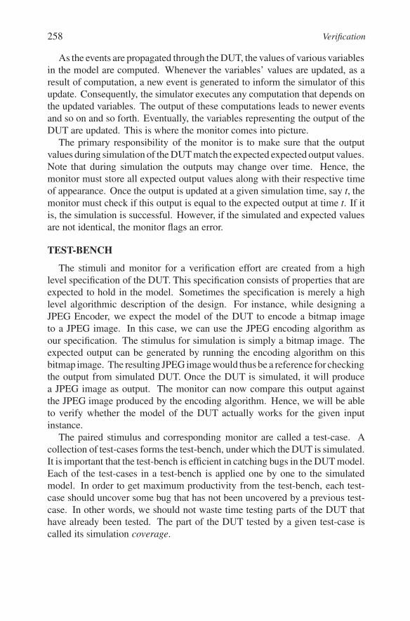
7.1 SIMULATION BASED METHODSSimulation is the most widely used method to verify system models. The

design to be tested is described in some modeling language and is referred to asdesign under test (DUT) as shown in Figure 7.1. The DUT sits in a simulationenvironment consisting of stimuli and monitors. The stimuli are a set of valuesthat are applied to the DUT’s inputs. These inputs then trigger a series of eventsand computations as described in the DUT model. It is the job of the simulatorto keep track of all these events and propagate them through the DUT. This isa scenario in a typical event-driven simulator.

DUT

Stim

ulus

Mon

itor

Simulator

Sp e c if ic ation

FIGURE 7.1 A typical simulation environment

258 Verification

As the events are propagated through the DUT, the values of various variablesin the model are computed. Whenever the variables’ values are updated, as aresult of computation, a new event is generated to inform the simulator of thisupdate. Consequently, the simulator executes any computation that depends onthe updated variables. The output of these computations leads to newer eventsand so on and so forth. Eventually, the variables representing the output of theDUT are updated. This is where the monitor comes into picture.

The primary responsibility of the monitor is to make sure that the outputvalues during simulation of the DUT match the expected expected output values.Note that during simulation the outputs may change over time. Hence, themonitor must store all expected output values along with their respective timeof appearance. Once the output is updated at a given simulation time, say t, themonitor must check if this output is equal to the expected output at time t. If itis, the simulation is successful. However, if the simulated and expected valuesare not identical, the monitor flags an error.

TEST-BENCHThe stimuli and monitor for a verification effort are created from a high

level specification of the DUT. This specification consists of properties that areexpected to hold in the model. Sometimes the specification is merely a highlevel algorithmic description of the design. For instance, while designing aJPEG Encoder, we expect the model of the DUT to encode a bitmap imageto a JPEG image. In this case, we can use the JPEG encoding algorithm asour specification. The stimulus for simulation is simply a bitmap image. Theexpected output can be generated by running the encoding algorithm on thisbitmap image. The resulting JPEG image would thus be a reference for checkingthe output from simulated DUT. Once the DUT is simulated, it will producea JPEG image as output. The monitor can now compare this output againstthe JPEG image produced by the encoding algorithm. Hence, we will be ableto verify whether the model of the DUT actually works for the given inputinstance.

The paired stimulus and corresponding monitor are called a test-case. Acollection of test-cases forms the test-bench, under which the DUT is simulated.It is important that the test-bench is efficient in catching bugs in the DUT model.Each of the test-cases in a test-bench is applied one by one to the simulatedmodel. In order to get maximum productivity from the test-bench, each test-case should uncover some bug that has not been uncovered by a previous test-case. In other words, we should not waste time testing parts of the DUT thathave already been tested. The part of the DUT tested by a given test-case iscalled its simulation coverage.

Simulation Based Methods 259

COVERAGEAlthough a rigorous definition of simulation coverage for a test-bench is

hard to come by, in general, it refers to the percentage of DUT that has beenchecked by the various tests applied during simulation. However, it is difficultto quantify a DUT. We can quantify it by the lines of source code for the modelwritten in some design language. Alternately, we can use a state diagram whichrepresents all possible scenarios that might exist during a model’s execution.The DUT can, thus, be quantified by the states and transitions in the statediagram. Unfortunately, these representations are incomplete and do not trulycapture the entire behavior of the design. The best bet in using coverage forgenerating new tests is to employ as many quantification metrics as possible.

We can use statement coverage to see how many lines of code were visitedduring a verification run. If during simulation with a given test-case, 100statements out of 1000 statements in the design were executed, then we say thatthe statement coverage for the test-case is 10%. However, this is a very weakmetric of coverage, since not all possible scenarios for those 100 statementswere exercised. For instance, the statement

a = b/c

will execute correctly if b = 4 and c = 2, but will cause an exception ifc = 0. Statement coverage would tell us if the given statement were executedduring simulation but not advise the user to check for the corner case of c = 0.

In the case of state coverage, we measure the number of states and transitionsthat are "traversed" during the model’s simulation. A state S is said to betraversed if during simulation of the DUT, S was visited at least once. Thiswould ensure that the scenario represented by s was tested during simulation.Hence, for the above example, if we were to cover the state with c = 0, wewould cover the overflow scenario. However, this would require that each legalvalue of c (and other variables) should have different states in the state diagram.Clearly, it will result in an unreasonably large state diagram.

PERFORMANCE IMPROVEMENTSIn an ideal scenario, one would like to run the minimum number of test cases

to cover as much of the design as possible. However, this would require somemethod to estimate the coverage of test-cases and generate the test bench in anefficient manner. In the absence of this kind of dynamic coverage feedback,the author of the test-bench may choose to randomly generate test-cases. Thismeans that the testing is not directed at finding specific bugs. Instead, thedesigner hopes that the random tests are fairly distributed in the range of possibleinputs. Naturally, the quality of such test-cases is in general poorer comparedto test-cases trying to cover particular scenarios.

260 Verification

The simulation performance can be improved by choosing test cases intelli-gently to maximize coverage with minimal simulation runs. One optimizationis to reduce test generation time by giving constraints to stimuli and testing withonly valid inputs. For instance, if we know from the design specification thata particular scenario is never going to occur, we do not need to spend time inwriting tests for such a scenario.

Besides stimulating the design with relevant test vectors, we can improveour understanding of the design by performing white box testing. In white boxtesting, we also monitor the non-primary output variables in the model. Ofcourse, such an approach only makes sense if the internal details of the designare available. Since we do not need to wait for the errors to be observed onthe primary outputs, the debug time is significantly reduced because the erroris usually observed close to its origin and this minimizes the effort neccessaryto locate the bug.

Another strategy to improve simulation performance is to speed up the sim-ulation itself. This is achieved by either using a faster simulation algorithm orusing hardware support for testing. For cycle accurate models of the design, itis sometimes possible to use a cycle simulation algorithm over the traditionalevent driven simulation algorithm. Since a cycle based algorithm does not takeinto account every event during a model’s execution, it avoids the overhead ofprocessing each event. In the case of hardware assisted testing, a functionalprototype of the design is implemented onto an FPGA. In some cases, part ofthe model can even be implemented on the FPGA and tested during the soft-ware simulation of the remaining design. This is achieved by using hardwareemulators capable of exchanging events with the software simulator.

The speed and efficiency of simulation is critical because the rise in complex-ity triggers a shift to a higher level of design description. We have witnessedthis in the shift from the transistor level to the gate level, RTL and now to thesystem level. By eliminating any unnecessary implementation details, we candescribe the behavior of the intended system in a succinct and efficient model.A system level modeling language aids such functional design. Its simulatorsare typically several orders faster than cycle accurate simulators. Since the ma-jority of design re-spins are due to functional errors, it is imperative that we firstfocus on getting the functionality of the design right, before implementing it.Hence, designs increasingly need to be modeled at higher levels of abstractionto leverage the simulation performance at the system level.

7.1.1 STIMULUS OPTIMIZATIONAnother way to optimize simulation is to test only those cases that the product

may actually encounter. Writing down all possible test vectors for simulationcan be a painful task. Also, generating test vectors randomly might result in

Simulation Based Methods 261

a lot of invalid vectors. Since the design is typically constrained to work foronly select scenarios, we can use this knowledge to generate only the valid testvectors. The test scenario can thus be written in some language and a tool can beused to generate valid test vectors for that scenario. Such languages are knownas verification languages. The key is to specify the property of the design to betested along with its description. These properties specify the behavior of thedesign using a formal language. For example, we may specify that the valueof variable y becomes 1, two clock cycles after variable x is set to 0. Then atest vector may be generated that sets x to 0 and observes the value of y aftertwo clock cycles. Therefore, we can automatically validate the assertion aboutthe behavior of the design. In short, the test generation tool analyzes the givenproperties and produces test vectors to validate those properties.

The constraints specified in the property lead to a set of legal inputs that formthe test pattern. Some times it is not necessary to have a different languageto do this because the properties can be embedded in the design model asspecial comments known as pragmas. The test generation tool can identifythese pragmas and produce tests based on them. However, for the synthesistool, the pragmas are merely comments and hence do not interfere with itsoperation.

Test G en er a to r

x zy x zy

C o v er a g eA n a l y si s

11

FIGURE 7.2 A test case that covers only part of the design.

Analyzing the results from coverage is another way to minimize the numberof test vectors. For instance, the code coverage feedback technique can bevisualized in Figure 7.2. A simulation of the model with input vector 11 resultsin only block x being covered. This is because block x is enabled by an ANDgate whose inputs are the two signals shown in the figure. The other two blocks,y and z, are enabled by the XOR and NAND of the inputs, respectively. Thus thecomputation inside y and z is not triggered by this test. The coverage analysistool thus comes back with the answer that only block x has been covered.

The designer analyzes the coverage result and comes up with a vector 10to cover blocks y and z. The enabling inputs to y and z are set to 1, thereby

262 Verification

Test G en er a to r

x zy x zy

C o v er a g eA n a l y si s

11

10

FIGURE 7.3 Coverage analysis results in a more useful test case.

enabling these blocks. Note that vector 00 would not cover block y and isthus not used. Therefore, the coverage feedback allows the designer to coverall blocks with just two input patterns. Without this knowledge, in the worstcase one would have to use all possible input combinations to achieve completecoverage. Although this is a simple and cosmetic example, it illustrates thebenefits of such a coverage feedback mechanism. Using the same principles,this strategy can be applied for other coverage metrics as well.

7.1.2 MONITOR OPTIMIZATIONAnother way to reduce the number of simulations is through beteer debugging

and design analysis methods [19]. Monitoring only the primary outputs of adesign during simulation lets us know if a bug exists. Tracing the bug to itssource can be difficult for complex designs. If the source code of the model isavailable, assertions can be placed on internal variables or signals in the model.For example, we can specify that the two complementary outputs of a flip-flopnever evaluate to the same value. Not only does this improve understandingof the design, it also points out the bug much closer to the source. Assertionscan also be used to check the validity of properties over time, such as protocolcompliance. However, the designer must ensure that the assertions do not getsynthesized along with the design. Therefore, they must be written either in alanguage different than the design, or as special comments that can be ignoredby the synthesis tool.

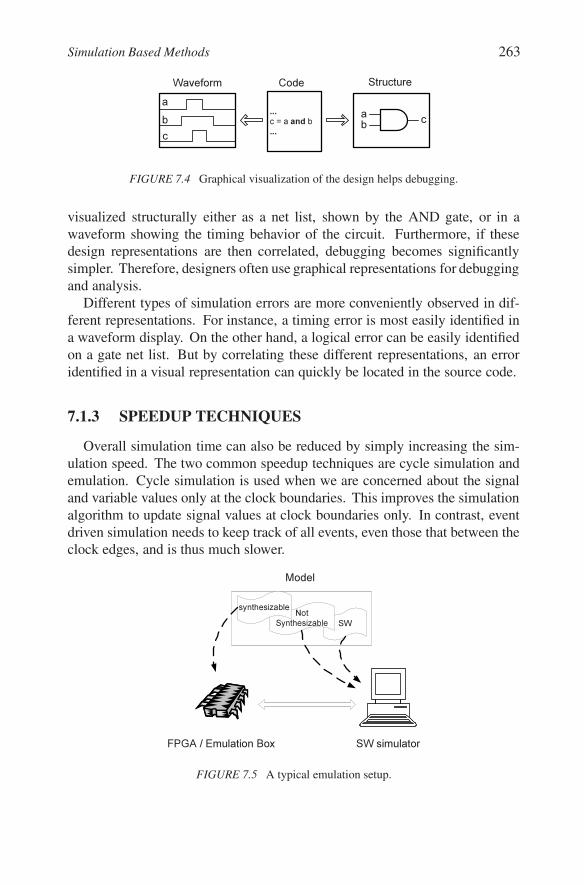
Graphical visualization of the structure and behavior of a design also helpsdebugging. Specifically, visually correlating different representations, such aswaveforms, net lists, state machines and code, allows the designer to easilyidentify design bugs and locate the source code for the errorneous part of themodel. As shown in Figure 7.4, the piece of code in a model source may be

Simulation Based Methods 263

...c = a a n d b...

Codeabc

ab c

S t r u ct u r eW av ef or m

FIGURE 7.4 Graphical visualization of the design helps debugging.

visualized structurally either as a net list, shown by the AND gate, or in awaveform showing the timing behavior of the circuit. Furthermore, if thesedesign representations are then correlated, debugging becomes significantlysimpler. Therefore, designers often use graphical representations for debuggingand analysis.

Different types of simulation errors are more conveniently observed in dif-ferent representations. For instance, a timing error is most easily identified ina waveform display. On the other hand, a logical error can be easily identifiedon a gate net list. But by correlating these different representations, an erroridentified in a visual representation can quickly be located in the source code.

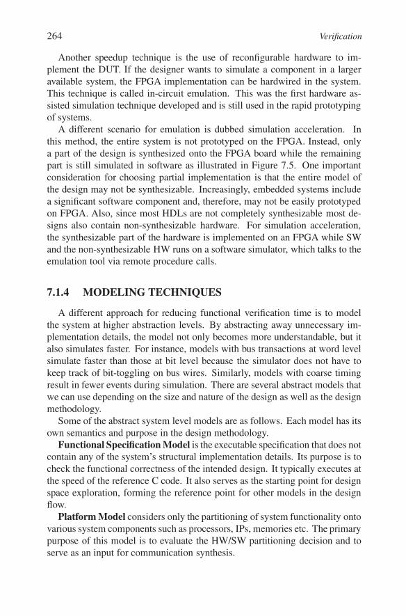
7.1.3 SPEEDUP TECHNIQUESOverall simulation time can also be reduced by simply increasing the sim-

ulation speed. The two common speedup techniques are cycle simulation andemulation. Cycle simulation is used when we are concerned about the signaland variable values only at the clock boundaries. This improves the simulationalgorithm to update signal values at clock boundaries only. In contrast, eventdriven simulation needs to keep track of all events, even those that between theclock edges, and is thus much slower.

SWN o t

Sy n t h e s i z a b l es y n t h e s i z a b l e

FPGA / E m u l a t i o n B o x S W s i m u l a t o r

M o d e l

FIGURE 7.5 A typical emulation setup.

264 Verification

Another speedup technique is the use of reconfigurable hardware to im-plement the DUT. If the designer wants to simulate a component in a largeravailable system, the FPGA implementation can be hardwired in the system.This technique is called in-circuit emulation. This was the first hardware as-sisted simulation technique developed and is still used in the rapid prototypingof systems.

A different scenario for emulation is dubbed simulation acceleration. Inthis method, the entire system is not prototyped on the FPGA. Instead, onlya part of the design is synthesized onto the FPGA board while the remainingpart is still simulated in software as illustrated in Figure 7.5. One importantconsideration for choosing partial implementation is that the entire model ofthe design may not be synthesizable. Increasingly, embedded systems includea significant software component and, therefore, may not be easily prototypedon FPGA. Also, since most HDLs are not completely synthesizable most de-signs also contain non-synthesizable hardware. For simulation acceleration,the synthesizable part of the hardware is implemented on an FPGA while SWand the non-synthesizable HW runs on a software simulator, which talks to theemulation tool via remote procedure calls.

7.1.4 MODELING TECHNIQUESA different approach for reducing functional verification time is to model

the system at higher abstraction levels. By abstracting away unnecessary im-plementation details, the model not only becomes more understandable, but italso simulates faster. For instance, models with bus transactions at word levelsimulate faster than those at bit level because the simulator does not have tokeep track of bit-toggling on bus wires. Similarly, models with coarse timingresult in fewer events during simulation. There are several abstract models thatwe can use depending on the size and nature of the design as well as the designmethodology.

Some of the abstract system level models are as follows. Each model has itsown semantics and purpose in the design methodology.

Functional Specification Model is the executable specification that does notcontain any of the system’s structural implementation details. Its purpose is tocheck the functional correctness of the intended design. It typically executes atthe speed of the reference C code. It also serves as the starting point for designspace exploration, forming the reference point for other models in the designflow.

Platform Model considers only the partitioning of system functionality ontovarious system components such as processors, IPs, memories etc. The primarypurpose of this model is to evaluate the HW/SW partitioning decision and toserve as an input for communication synthesis.

Formal Verification Methods 265

Transaction Level Model contains the communication structure of the in-tended design along with the HW/SW partitioning. The communication, how-ever, is not yet pin accurate. Since we are only interested in the approximatetiming of communication, the data transfers between components are modeledas abstract bus transactions.

These abstract system level models need not be the only ones used in a designflow. Depending on the application and design characteristics, different modelsmay also be employed. However, the guiding principle in choosing such modelsis the simulation speed and the possibility for design space exploration.

7.2 FORMAL VERIFICATION METHODSFormal verification techniques use mathematical formulations to verify de-

signs [113]. The key difference from simulation based verification is the ab-sence of a test pattern. The formal verification process either compares two dif-ferent models of the design or shows that a property is satisfied on the model. Ineither case the answer from the formal verification tool is valid for all scenarios.This is one of the strongest points of formal methods; they can provide abso-lute answers to verification problems. On the flip side, however, most formaltechniques involve converting the model to some abstract mathematical form,which may not always be feasible.

In the design industry, there are three primary types of formal verification.The first is equivalence checking, which can be used to compare two models.In general, equivalence checking can establish whether two models will givethe same result under all possible inputs. This is particularly useful in checkingthe correctness of the synthesis and optimization steps. Due to the critical im-portance of model correctness, the designer cannot trust the synthesis tools topreserve all the properties of the original model. Hence, equivalence checkingactually serves a validation of the synthesis step. For the purpose of equiva-lence checking, one needs to define some notion of model equivalence suchas logical equivalence or state machine equivalence. Based on this notion, theequivalence checker then proves or disproves the equivalence of the originaland optimized/synthesized models.

Model checking, on the other hand, takes a formal representation of boththe model and a given property and checks if the property is satisfied by themodel. More often than not, system models become too big or complicated atlower levels of abstraction. Hence, their behavior needs to be checked againstsome abstract specification. This abstract specification is essentially a set ofproperties that are expected to hold on the model. These properties are similarto the one described in Section 7.1. A model checking tool can automaticallyverify if each of these properties holds in the model. Most modern assertion

266 Verification

based verification tools, compose these abstract properties from assertions in themodel and use them for model checking. The properties are temporal in nature,i.e. they define the behavior of the system over time. A complete theory oftemporal logic forms the framework on which model checking is based. Theseproperties are written as formulas in the temporal logic and the model checkertries to prove or disprove each formula.

A somewhat different approach in formal verification, known as theoremproving, tries to prove properties under some mathematical logic by using de-ductive reasoning. Theorem proving has the advantage of being applicable toalmost any domain of problems and is hence very versatile. This flexibility isalso a reason for its biggest disadvantage: it is extremely hard to create auto-mated tools for theorem proving. The basic idea behind theorem proving is toexpress both the specification and the implementation models as mathematicalformulas. On the basis of axioms, which are established truths in the given logic,one can show the equality of the two formulas. Hence, the proof establishesthat the implementation model is a valid substitution for the specification.

In this section we will look at all these formal verification methods in detail.

inputs

outpu

tsregister/b l a c k b o x

register/b l a c k b o x

12

inputs

outpu

tsregister/b l a c k b o x

register/b l a c k b o x

1'2'

… … .1 = 1' ?2 = 2' ?… … ..

Original Model

Op t im iz ed Model

E q u iv alenc eC h ec k er

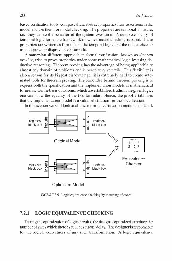
FIGURE 7.6 Logic equivalence checking by matching of cones.

7.2.1 LOGIC EQUIVALENCE CHECKINGDuring the optimization of logic circuits, the design is optimized to reduce the

number of gates which thereby reduces circuit delay. The designer is responsiblefor the logical correctness of any such transformation. A logic equivalence

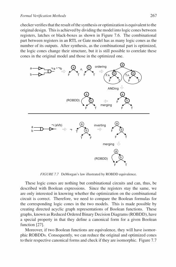
Formal Verification Methods 267

checker verifies that the result of the synthesis or optimization is equivalent to theoriginal design. This is achieved by dividing the model into logic cones betweenregisters, latches or black-boxes as shown in Figure 7.6. The combinationalpart between registers in an RTL or Gate model has as many logic cones as thenumber of its outputs. After synthesis, as the combinational part is optimized,the logic cones change their structure, but it is still possible to correlate thesecones in the original model and those in the optimized one.

a bF T F T

a

a

b

b

a ^ b

(aV b)

a

bF T

F bF T

T

b

F T

aFb

F T

a

bT F

a

T bF T

aF

b

F T

a

A N D i n g

o r d e r i n g

m e r g i n g

m e r g i n g

i n v e r t i n g

(R O B D D )

(R O B D D )

FIGURE 7.7 DeMorgan’s law illustrated by ROBDD equivalence.

These logic cones are nothing but combinational circuits and can, thus, bedescribed with Boolean expressions. Since the registers stay the same, weare only interested in knowing whether the optimization on the combinationalcircuit is correct. Therefore, we need to compare the Boolean formulas forthe corresponding logic cones in the two models. This is made possible bycreating directed acyclic graph representations of Boolean functions. Thesegraphs, known as Reduced Ordered Binary Decision Diagrams (ROBDD), havea special property in that they define a canonical form for a given Booleanfunction [27].

Moreover, if two Boolean functions are equivalence, they will have isomor-phic ROBDDs. Consequently, we can reduce the original and optimized conesto their respective canonical forms and check if they are isomorphic. Figure 7.7

268 Verification

illustrates this principle on the DeMorgan’s law for Boolean functions, whichstates

!(a + b) = (!a).(!b)

So ROBDDs are a compact way of representing Boolean functions. Fur-thermore, all Boolean functions, such as conjunction (AND), disjunction (OR),and negation (NOT) may be expressed as graph manipulations of ROBDDs.Other graph manipulations, such as merging, are used to reduce the BDDs intocanonical form. Some of these graph manipulations are shown in Figure 7.7 inthe construction of the ROBDDs for the LHS and RHS of the DeMorgan equa-tion. Note that these ROBDDs are isomorphic. The seminal paper by Bryantintroduces ROBDDs and their manipulation for logic equivalence checking. Inlogic equivalence checking, isomorphic ROBDDs ensure that an optimizationof the logic circuit is functionality preserving.

7.2.2 FSM EQUIVALENCE CHECKINGA logic equivalence checker verifies the equivalence of only the combina-

tional part of the circuit. There are also techniques to check equivalence of thesequential part of the design [135]. In order to understand those techniques,we have to define the notion of a finite state machine. A finite state machine(FSM), as described in Section 3.1.2, is a tuple consisting of a set of inputs, a setof outputs, and a set of states. Some of the states are designated as initial statesand some as final states. Transitions between states are defined as a functionof the current state and the input. An output is also associated with every state.Formally, we can define a FSM as the tuple

< I,O,Q,Q0, F,H >,where

I is the set of inputs O is the set of outputs Q is the set of states Q0 is theset of initial states F is the state transition function Q X I  Q H is the outputfunction Q  O

We may think of a FSM as a language acceptor. We further define Qf as theset of final states. If we start from an initial state (in Q0), supply input symbolsfrom a string S and reach a final state, then S is said to be accepted by the FSM.The set of all acceptable strings forms the language of the FSM.

We can also define the notion of a FSM product. The product of two FSMsM1 and M2 has the same behavior as if M1 and M2 were running in parallel.Therefore, given FSMs M1 and M2, such that

M1 : < I,O1, Q1, Q01, F1,H1 >,

M2 : < I,O2, Q2, Q02, F2,H2 >

Formal Verification Methods 269

The product FSM M1 ∗M2 may be written asM1 ∗M2 : < I,O1UO2, Q1XQ2, QO1XQO2, F1XF2,H1XH2 > .

The total number of states in the resulting machine is the product of thenumber of states in each machine. The product machine carries all possiblepairs of states, one from each of the two input machines. The paired statesare labeled with the pair of corresponding outputs as well. The inputs on thetransition arcs are also pairs of possible inputs from each machine.

Using the above definitions, we can define sequential equivalence of FSMmodels through a simple metric. We must prove that if two FSMs are giventhe same inputs in the same sequence, then under no circumstances would theyproduce different outputs [48]. Only then can we claim that the machinesare equivalent. The specification and its implementation are both representedas FSMs Ms and Mi respectively. We must ensure that the input and outputalphabet of the two machines is the same.

p

q

x

y

r

s

x

y

ty

pr ps pt

qtqs qr

xx xy xy

yxyy yy

a

b

a

b b

aa bb

bb

x

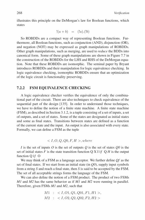
FIGURE 7.8 Equivalence checking of sequential design using product FSMs.

To perform FSM equivalence checking, we first derive the product machineMsXMi. Now all the states in MsXMi that have a pair of differing outputsare labeled as final states as shown in Figure 7.8. Ms has two states, p and q,while Mi has three states, r, s, and t. States p and r produce output x while theother three states generate output y. Therefore, in the FSM product, the statesps, pt and qr have output pairs with different symbols (xy or yx) and are thuslabeled as final states. We also keep only those transitions that have the samesymbols in the input pair. What we are trying to prove is that for the samesequence of inputs, Ms and Mi would produce the same sequence of outputs. Inother words, we should never reach a state with a pair of non-identical outputs.Since such states are the final states in the product FSM, they should never bereached if Ms and Mi are equivalent. Therefore the product FSM should notaccept any language.

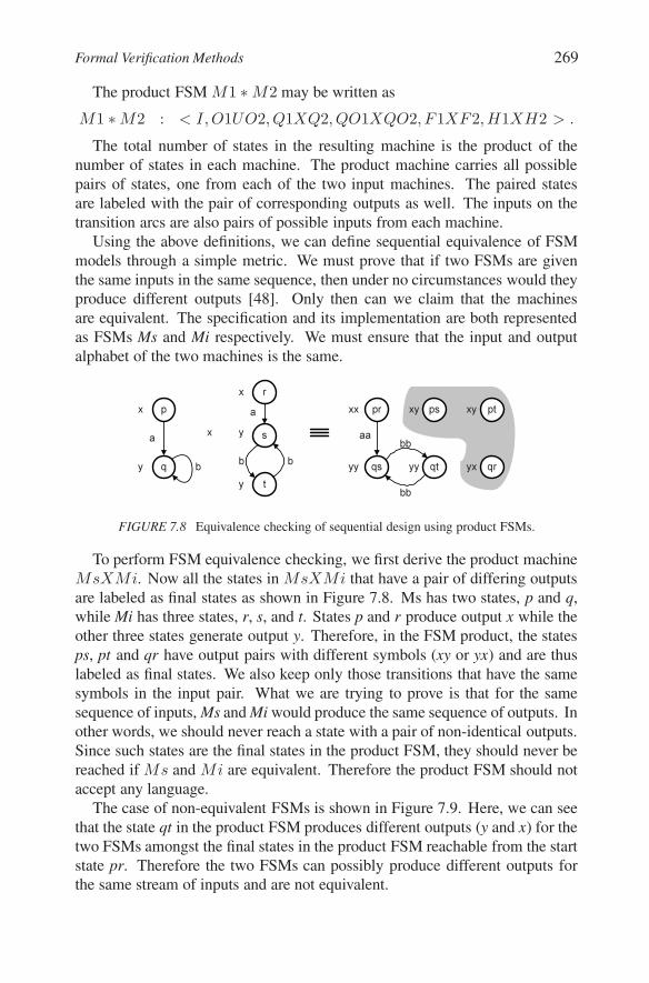
The case of non-equivalent FSMs is shown in Figure 7.9. Here, we can seethat the state qt in the product FSM produces different outputs (y and x) for thetwo FSMs amongst the final states in the product FSM reachable from the startstate pr. Therefore the two FSMs can possibly produce different outputs forthe same stream of inputs and are not equivalent.

270 Verification

p

q

x

y

r

s

x

y

tx

pr ps pt

qtqs qr

xx xy xy

yxyy yx

a

b

a

b b

aa bb

bb

x

FIGURE 7.9 Product FSM for with a reachable error state.

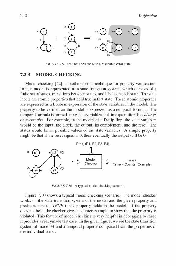
7.2.3 MODEL CHECKINGModel checking [42] is another formal technique for property verification.

In it, a model is represented as a state transition system, which consists of afinite set of states, transitions between states, and labels on each state. The statelabels are atomic properties that hold true in that state. These atomic propertiesare expressed as a Boolean expression of the state variables in the model. Theproperty to be verified on the model is expressed as a temporal formula. Thetemporal formula is formed using state variables and time quantifiers like alwaysor eventually. For example, in the model of a D-flip flop, the state variableswould be the input, the clock, the output, its complement, and the reset. Thestates would be all possible values of the state variables. A simple propertymight be that if the reset signal is 0, then eventually the output will be 0.

s1 s2

s3s4

P1

P4 P3

P2M o d e l

C h e c k e r

P = f (P1, P2, P3, P4)

T r u e /F a l se + C o u n t e r E x a m p l e

T

FIGURE 7.10 A typical model checking scenario.

Figure 7.10 shows a typical model checking scenario. The model checkerworks on the state transition system of the model and the given property andproduces a result TRUE if the property holds in the model. If the propertydoes not hold, the checker gives a counter-example to show that the property isviolated. This feature of model checking is very helpful in debugging becauseit provides a readymade test case. In the given figure, we see the state transitionsystem of model M and a temporal property composed from the properties ofthe individual states.

Formal Verification Methods 271

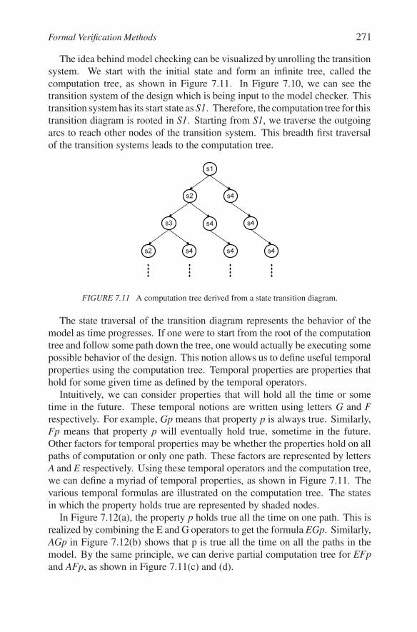
The idea behind model checking can be visualized by unrolling the transitionsystem. We start with the initial state and form an infinite tree, called thecomputation tree, as shown in Figure 7.11. In Figure 7.10, we can see thetransition system of the design which is being input to the model checker. Thistransition system has its start state as S1. Therefore, the computation tree for thistransition diagram is rooted in S1. Starting from S1, we traverse the outgoingarcs to reach other nodes of the transition system. This breadth first traversalof the transition systems leads to the computation tree.

s1

s2 s4

s3 s4 s4

s2 s4 s4 s4

FIGURE 7.11 A computation tree derived from a state transition diagram.

The state traversal of the transition diagram represents the behavior of themodel as time progresses. If one were to start from the root of the computationtree and follow some path down the tree, one would actually be executing somepossible behavior of the design. This notion allows us to define useful temporalproperties using the computation tree. Temporal properties are properties thathold for some given time as defined by the temporal operators.

Intuitively, we can consider properties that will hold all the time or sometime in the future. These temporal notions are written using letters G and Frespectively. For example, Gp means that property p is always true. Similarly,Fp means that property p will eventually hold true, sometime in the future.Other factors for temporal properties may be whether the properties hold on allpaths of computation or only one path. These factors are represented by lettersA and E respectively. Using these temporal operators and the computation tree,we can define a myriad of temporal properties, as shown in Figure 7.11. Thevarious temporal formulas are illustrated on the computation tree. The statesin which the property holds true are represented by shaded nodes.

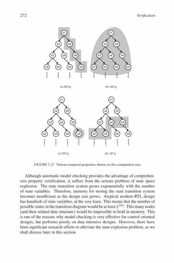
In Figure 7.12(a), the property p holds true all the time on one path. This isrealized by combining the E and G operators to get the formula EGp. Similarly,AGp in Figure 7.12(b) shows that p is true all the time on all the paths in themodel. By the same principle, we can derive partial computation tree for EFpand AFp, as shown in Figure 7.11(c) and (d).

272 Verification

s1

s2 s4

s3 s4 s4

s2 s4 s4 s4

(a) EG p

s1

s2 s4

s3 s4 s4

s2 s4 s4 s4

(b) AG p

s1

s2 s4

s3 s4 s4

s2 s4 s4 s4

(c) EF p

s1

s2 s4

s3 s4 s4

s2 s4 s4 s4

(d) AF p

FIGURE 7.12 Various temporal properties shown on the computation tree.

Although automatic model checking provides the advantage of comprehen-sive property veriification, it suffers from the serious problem of state spaceexplosion. The state transition system grows exponentially with the numberof state variables. Therefore, memory for storing the state transition systembecomes insufficient as the design size grows. Atypical modern RTL designhas hundreds of state variables, at the very least. This means that the number ofpossible states in the transition diagram would be at least 2100. This many nodes(and their related data structure) would be impossible to hold in memory. Thisis one of the reasons why model checking is very effective for control orienteddesigns, but performs poorly on data intensive designs. However, there havebeen significant research efforts to alleviate the state explosion problem, as weshall discuss later in this section.

Formal Verification Methods 273

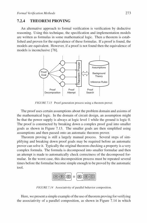
7.2.4 THEOREM PROVINGAn alternative approach to formal verification is verification by deductive

reasoning. Using this technique, the specification and implementation modelsare written as formulas in some mathematical logic. Then a theorem is estab-lished and proven for the equivalence of these formulas. If a proof is found, themodels are equivalent. However, if a proof is not found then the equivalence ofmodels is inconclusive [78].

ProofG oa l

Theo

rem Prove

r

ProofA t t e m p t

ProofD e c om p os i t i on

A s s u m p t i on sB a c k g rou n d

T h e oryI n fe re n c e R u l e s

ProofS e a rc h

FIGURE 7.13 Proof generation process using a theorem prover.

The proof uses certain assumptions about the problem domain and axioms ofthe mathematical logic. In the domain of circuit design, an assumption mightbe that the power supply is always at logic level 1 while the ground is logic 0.The proof is constructed by breaking down a complex proof goal into smallergoals as shown in Figure 7.13. The smaller goals are then simplified usingassumptions and then passed onto an automatic theorem prover.

Theorem proving is still a largely manual process. Several steps of sim-plifying and breaking down proof goals may be required before an automaticprover can solve it. Typically the original theorem checking a property is a verycomplex formula. The formula is decomposed into smaller formulae and thenan attempt is made to automatically check correctness of the decomposed for-mulae. In the worst case, this decomposition process must be repeated severaltimes before the formulae become simple enough to be proved by the automatictool.

CBAA CB

FIGURE 7.14 Associativity of parallel behavior composition.

Here, we present a simple example of the use of theorem proving for verifyingthe associativity of a parallel composition, as shown in Figure 7.14 in which

274 Verification

parallel behaviors A, B, C are combined in two different fashions. On the leftside, behaviors A and B are combined into a parallel behavior which is thencombined into another parallel behavior with C. On the right side, behaviors Band C are combined first and the resulting behavior is then combined with A.The example demonstrates the basic principle of associativity as applied to theparallel composition of behaviors.

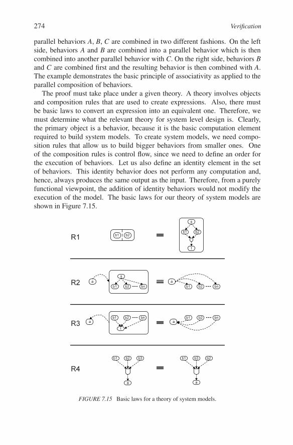
The proof must take place under a given theory. A theory involves objectsand composition rules that are used to create expressions. Also, there mustbe basic laws to convert an expression into an equivalent one. Therefore, wemust determine what the relevant theory for system level design is. Clearly,the primary object is a behavior, because it is the basic computation elementrequired to build system models. To create system models, we need compo-sition rules that allow us to build bigger behaviors from smaller ones. Oneof the composition rules is control flow, since we need to define an order forthe execution of behaviors. Let us also define an identity element in the setof behaviors. This identity behavior does not perform any computation and,hence, always produces the same output as the input. Therefore, from a purelyfunctional viewpoint, the addition of identity behaviors would not modify theexecution of the model. The basic laws for our theory of system models areshown in Figure 7.15.

R1

b1 b2

sa

bn b1 b2a

bnR2

b1 b2

t

abn b1 b2

abn

R3

a

b1 b2 b3

R4a

b1 b3 b2

b2b1

t

b1 b2

s

FIGURE 7.15 Basic laws for a theory of system models.

Formal Verification Methods 275

With these laws in place, the proof process takes the implementation formulaand reduces it to the specification formula by a number of proof steps. Eachproof step uses an assumption, an axiom, or an already proven theorem. Inour case, the axioms are the laws as shown in Figure 7.15. Our proof goalis to show the equivalence of parallel compositions under associativity. If thefunction par(b1; b2 ::: bn) represents a parallel composition of n behaviors, wecan write our proof goal as the following equation:

par(par(a; b); c) = par(a; par(b; c))

The proof steps use the basic laws of our theory, as presented earlier, totransform the expression on the RHS into the expression on the LHS.

7.2.5 DRAWBACKS OF FORMAL VERIFICATIONCompared to simulation based methods, formal verification methods have

not been as well accepted in the industry due to several drawbacks. Logicalequivalence checking works only for combinational logic while FSM equiva-lence checking requires both the pecification and implementation machines tohave the same set of inputs and outputs.

Model checking, besides suffering from the state explosion problem, is notsuitable for all types of designs. Since it needs a state transition system, it worksbest for control intensive designs such as bus controllers. Automatic theoremproving has not become very popular in the industry either; the foremost reasonfor this is the amount of manual intervention required in running the theoremproving. Since different applications have different kinds of assumptions andproof strategies, it is infeasible for a theorem proving tool to generate the entireproof automatically. Secondly, most designers lack a background in mathemat-ical logic. Therefore, it requires a huge investment and long training time forthem to start using theorem proving efficiently.

7.2.6 IMPROVEMENTS TO FORMAL VERIFICATIONMETHODS

Recently, tools vendors and academics have made several improvements toformal techniques, particularly in model checking. Symbolic model check-ing [136] encodes the state transition system using BDDs, which is a muchmore compact representation than exhaustively enumerating the states and tran-sitions. Since BDDs represent sets of states, the model checking algorithm canoperate on sets of states rather than individual states.

Another innovation is bounded model checking, which checks if a modelsatisfies a property on paths of length at most K. The number K is incremented

276 Verification

until a bug is found or the problem becomes intractable. Partial order reductiontechniques are usually used in model checking for asynchronous systems, inwhich concurrent tasks are interleaved rather than executed simultaneously. Ituses the commutativity of concurrently executed transitions, which result in thesame state when executed in different orders.

Abstraction technique is used to create smaller state transition graphs. Thespecified property is described using some state variables. The variables thatdo not influence the specified property are eliminated from the model, therebypreserving the property while reducing the model size.

7.2.7 SEMI-FORMAL METHODS: SYMBOLICSIMULATION

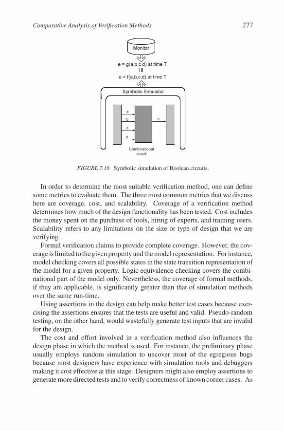
Semi-formal verification refers to the ues of formalisms and formal verifica-tion methods in a simulation environment. The idea behind symbolic simulationis to significantly minimize the number of simulation test vectors by using sym-bols to achieve the same coverage. In symbolic simulation, the stimulus appliesBoolean variables as inputs to the simulation model. This is illustrated in Fig-ure 7.16. During simulation, the internal variables and outputs are computed asBoolean expressions. In order to check for correctness, the output expressionis compared with the expected output expression as defined by the Monitor.BDDs can be used to store the Boolean expressions in the Monitor. The BDDsof equivalent Boolean expressions can be reduced to identical canonical forms.Therefore, the equivalence of a specified output expression to a simulated out-put expression can be checked easily. For larger circuits, in which the BDDsize may blow up, we can use SAT solvers as is increasingly common.

7.3 COMPARATIVE ANALYSIS OF VERIFICATIONMETHODS

Different application domains and types of systems may require differentverification methods. Formal methods, though time consuming and difficult todeploy, may be needed for ASIC implementation of mission-critical systemsor processors because of the thoroughness of the verification they perform. Onthe other hand, inexpensive reconfigurable devices may not require such ex-haustiveness, so randomized simulation may be sufficient. It is important toconsider how to best introduce verification in a system design flow. Depend-ing on the abstraction level of the models and the application characteristics,different verification techniques may be employed.

Comparative Analysis of Verification Methods 277

Monitor

Combinational cir cu it

a

b

c

d

e

S y m bol ic S im u l ator

e = f(a,b,c,d) at tim e T

e = g(a,b,c,d) at tim e T

FIGURE 7.16 Symbolic simulation of Boolean circuits.

In order to determine the most suitable verification method, one can definesome metrics to evaluate them. The three most common metrics that we discusshere are coverage, cost, and scalability. Coverage of a verification methoddetermines how much of the design functionality has been tested. Cost includesthe money spent on the purchase of tools, hiring of experts, and training users.Scalability refers to any limitations on the size or type of design that we areverifying.

Formal verification claims to provide complete coverage. However, the cov-erage is limited to the given property and the model representation. For instance,model checking covers all possible states in the state transition representation ofthe model for a given property. Logic equivalence checking covers the combi-national part of the model only. Nevertheless, the coverage of formal methods,if they are applicable, is significantly greater than that of simulation methodsover the same run-time.

Using assertions in the design can help make better test cases because exer-cising the assertions ensures that the tests are useful and valid. Pseudo-randomtesting, on the other hand, would wastefully generate test inputs that are invalidfor the design.

The cost and effort involved in a verification method also influences thedesign phase in which the method is used. For instance, the preliminary phaseusually employs random simulation to uncover most of the egregious bugsbecause most designers have experience with simulation tools and debuggersmaking it cost effective at this stage. Designers might also employ assertions togenerate more directed tests and to verify correctness of known corner cases. As

278 Verification

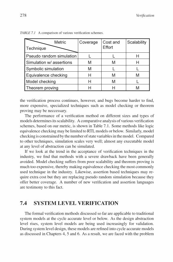
TABLE 7.1 A comparison of various verification schemes.

LLMS y m b o l i c s i m u l a t i o nMMHE q u i v a l e n c e c h e c k i n gLMHMo d e l c h e c k i n gMHHT h e o r e m p r o v i n g

HMMS i m u l a t i o n w / a s s e r t i o n sHLLP s e u d o r a n d o m s i m u l a t i o n

S c a l a b i l i t yC o s t a n d E f f o r t

C o v e r a g eMe t r i cT e c h n i q u e

the verification process continues, however, and bugs become harder to find,more expensive, specialized techniques such as model checking or theoremproving may be neccessary.

The performance of a verification method on different sizes and types ofmodels determines its scalability. A comparative analysis of various verificationschemes, based on our metric, is shown in Table 7.1. Some methods like logicequivalence checking may be limited to RTL models or below. Similarly, modelchecking is constrained by the number of state variables in the model. Comparedto other techniques, simulation scales very well; almost any executable modelat any level of abstraction can be simulated.

If we look at the trend in the acceptance of verification techniques in theindustry, we find that methods with a severe drawback have been generallyavoided. Model checking suffers from poor scalability and theorem proving ismuch too expensive, thereby making equivalence checking the most commonlyused technique in the industry. Likewise, assertion based techniques may re-quire extra cost but they are replacing pseudo random simulation because theyoffer better coverage. A number of new verification and assertion languagesare testimony to this fact.

7.4 SYSTEM LEVEL VERIFICATIONThe formal verification methods discussed so far are applicable to traditional

system models at the cycle accurate level or below. As the design abstractionlevel rises, system level models are being used increasingly for validation.During system level design, these models are refined into cycle accurate modelsas discussed in Chapters 4, 5 and 6. As a result, we are faced with the problem

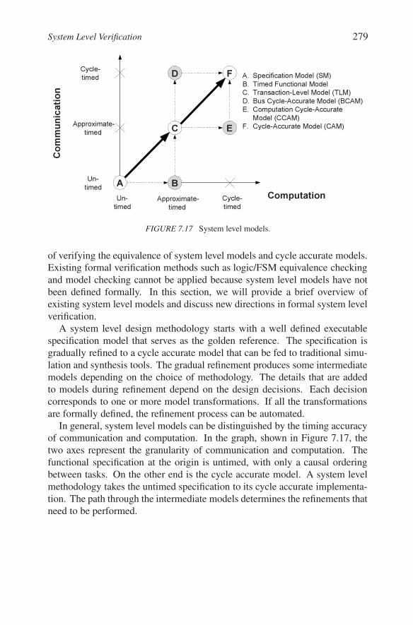
System Level Verification 279

Computation

Commun

ication

A B

C

D F

Un-t i m e d

A p p r o x i m a t e -t i m e d

C y c l e -t i m e d

Un-t i m e d

A p p r o x i m a t e -t i m e d E

C y c l e -t i m e d A . S p e c i f i c a t i o n M o d e l ( S M )

B . T i m e d F u nc t i o na l M o d e lC . T r a ns a c t i o n-L e v e l M o d e l ( T L M )D . B u s C y c l e -A c c u r a t e M o d e l ( B C A M )E . C o m p u t a t i o n C y c l e -A c c u r a t e

M o d e l ( C C A M )F . C y c l e -A c c u r a t e M o d e l ( C A M )

FIGURE 7.17 System level models.

of verifying the equivalence of system level models and cycle accurate models.Existing formal verification methods such as logic/FSM equivalence checkingand model checking cannot be applied because system level models have notbeen defined formally. In this section, we will provide a brief overview ofexisting system level models and discuss new directions in formal system levelverification.

A system level design methodology starts with a well defined executablespecification model that serves as the golden reference. The specification isgradually refined to a cycle accurate model that can be fed to traditional simu-lation and synthesis tools. The gradual refinement produces some intermediatemodels depending on the choice of methodology. The details that are addedto models during refinement depend on the design decisions. Each decisioncorresponds to one or more model transformations. If all the transformationsare formally defined, the refinement process can be automated.

In general, system level models can be distinguished by the timing accuracyof communication and computation. In the graph, shown in Figure 7.17, thetwo axes represent the granularity of communication and computation. Thefunctional specification at the origin is untimed, with only a causal orderingbetween tasks. On the other end is the cycle accurate model. A system levelmethodology takes the untimed specification to its cycle accurate implementa-tion. The path through the intermediate models determines the refinements thatneed to be performed.

280 Verification

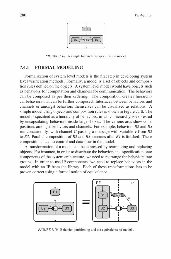
B2 B3cv v

B1

FIGURE 7.18 A simple hierarchical specification model.

7.4.1 FORMAL MODELINGFormalization of system level models is the first step in developing system

level verification methods. Formally, a model is a set of objects and composi-tion rules defined on the objects. A system level model would have objects suchas behaviors for computation and channels for communication. The behaviorscan be composed as per their ordering. The composition creates hierarchi-cal behaviors that can be further composed. Interfaces between behaviors andchannels or amongst behaviors themselves can be visualized as relations. Asimple model using objects and composition rules is shown in Figure 7.18. Themodel is specified as a hierarchy of behaviors, in which hierarchy is expressedby encapsulating behaviors inside larger boxes. The various arcs show com-positions amongst behaviors and channels. For example, behaviors B2 and B3run concurrently, with channel C passing a message with variable v from B2to B3. Parallel composition of B2 and B3 executes after B1 is finished. Thesecompositions lead to control and data flow in the model.

A transformation of a model can be expressed by rearranging and replacingobjects. For instance, in order to distribute the behaviors in a specification ontocomponents of the system architecture, we need to rearrange the behaviors intogroups. In order to use IP components, we need to replace behaviors in themodel with an IP from the library. Each of these transformations has to beproven correct using a formal notion of equivalence.

B2 B3cv v

s y n c00

P E I P

B2 B3cv v

B1B1

FIGURE 7.19 Behavior partitioning and the equivalence of models.

System Level Verification 281

Intuitively, we can draw an analogy between the distributive law for natu-ral numbers and the ‘distribution of behaviors on different components. Thedistribution of multiplication over addition can be written as:

a ∗ (b + c) = a ∗ b + a ∗ c

This forms a basic axiom in the theory of natural numbers. Just as theexpression on the LHS is equal to that on the RHS in the distributive lawequation, we can demonstrate that a model on the LHS is equal to a model onthe RHS in Figure 7.19. The model on the LHS has a sequential compositionof a leaf level behavior B1 and a hierarchical concurrent composition of B andB3. Channel c is used to send data from B2 to B3. On the RHS, the model istransformed to create a concurrent composition at the top level by isolating B3into the independent behavior IP. However, the syntactic transformation doesnot change the function of the model. The equality is determined by the orderin which the behaviors execute.

PE

c1

I P

c3

c2

c2PE I P

c1c2

c1c2

B u s 1

B u s 2

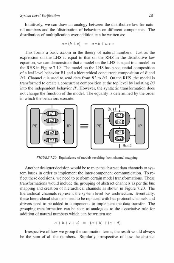
FIGURE 7.20 Equivalence of models resulting from channel mapping.

Another designer decision would be to map the abstract data channels to sys-tem buses in order to implement the inter-component communication. To re-flect these decisions, we need to perform certain model transformations. Thesetransformations would include the grouping of abstract channels as per the busmapping and creation of hierarchical channels as shown in Figure 7.20. Thehierarchical channels represent the system level bus architecture. Eventually,these hierarchical channels need to be replaced with bus protocol channels anddrivers need to be added in components to implement the data transfer. Thegrouping transformation can be seen as analogous to the associative rule foraddition of natural numbers which can be written as:

a + b + c + d = (a + b) + (c + d)

Irrespective of how we group the summation terms, the result would alwaysbe the sum of all the numbers. Similarly, irrespective of how the abstract

282 Verification

channels are grouped in the transformed model, they would perform the samedata transactions as in the original model.

The system level verification problem is to determine if the model refine-ments used to create a cycle accurate model from a system level model arefunctionality preserving. This can be achieved by creating by formalizing sys-tem level models and defining functionality preserving transformation rules.Next, each model refinement can be expressed as a well defined sequence oftransformations. If each transformation is proved to be functionality preserv-ing, the refinement will produces an output model that is equivalent to the inputmodel. Using this technique we can solve the system level verification problem.

Let us now look at a formalism for system level models, called Model Alge-bra, that enables system level verification.

7.4.2 MODEL ALGEBRAModel algebra [1] is a formalism for the representation and symbolic trans-

formation of system level models. In model algebra, a system can be viewedas a block of computation with inputs and outputs for stimuli and responses.This computation block is composed of smaller computation blocks that exe-cute in a given order and communicate with each other. Therefore, objects forcomputation and communication are defined in model algebra. The computa-tion objects are referred to as behaviors. A behavior has ports that allow it tocommunicate with other behaviors and to create hierarchical composition of be-haviors. The primitives for communication are variables and channels. Thesecommunication objects have different semantics. Variables allow a "read, com-pute and store" style of communication, while channels support a synchronizedhandshake style of communication. Composition rules are used to create anexecution order for behaviors and to bind their ports to either variables or chan-nels. In model algebra, a system is thus represented as a hierarchical behaviorcomposed of sub-behaviors communicating via variables and channels. Theobjects of model algebra can be defined using the tuple

< B,C, V, I, P,A >

in which B is the set of behaviors, C is the set of channels, V is the set ofvariables, I is the behavior interface, P is the set of behavior ports, and A is theset of address labels for links that go over channels. We also define a subsetof B representing the set of identity behaviors. Identity behaviors are thosebehaviors that, upon execution, produce an output which is identical to theirinput. We further define Q to be the subset of V such that all variables in Q areof type Boolean.

System Level Verification 283

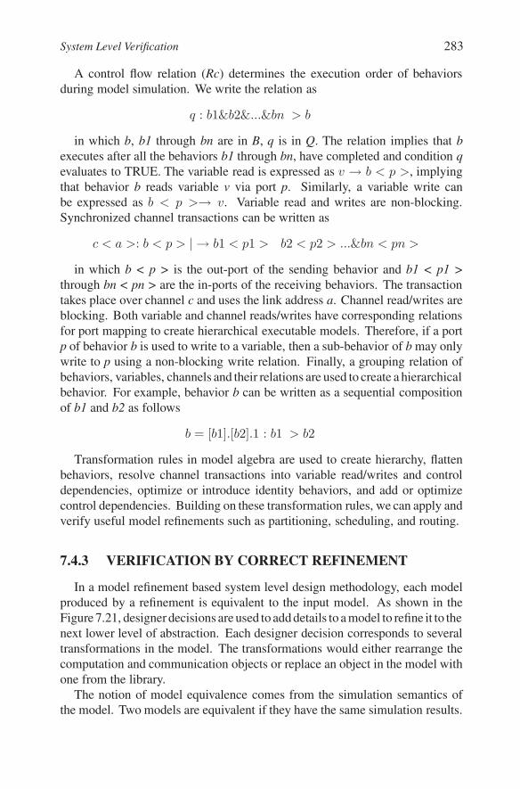
A control flow relation (Rc) determines the execution order of behaviorsduring model simulation. We write the relation as

q : b1&b2&...&bn > b

in which b, b1 through bn are in B, q is in Q. The relation implies that bexecutes after all the behaviors b1 through bn, have completed and condition qevaluates to TRUE. The variable read is expressed as v → b < p >, implyingthat behavior b reads variable v via port p. Similarly, a variable write canbe expressed as b < p >→ v. Variable read and writes are non-blocking.Synchronized channel transactions can be written as

c < a >: b < p > | → b1 < p1 > b2 < p2 > ...&bn < pn >

in which b < p > is the out-port of the sending behavior and b1 < p1 >through bn < pn > are the in-ports of the receiving behaviors. The transactiontakes place over channel c and uses the link address a. Channel read/writes areblocking. Both variable and channel reads/writes have corresponding relationsfor port mapping to create hierarchical executable models. Therefore, if a portp of behavior b is used to write to a variable, then a sub-behavior of b may onlywrite to p using a non-blocking write relation. Finally, a grouping relation ofbehaviors, variables, channels and their relations are used to create a hierarchicalbehavior. For example, behavior b can be written as a sequential compositionof b1 and b2 as follows

b = [b1].[b2].1 : b1 > b2

Transformation rules in model algebra are used to create hierarchy, flattenbehaviors, resolve channel transactions into variable read/writes and controldependencies, optimize or introduce identity behaviors, and add or optimizecontrol dependencies. Building on these transformation rules, we can apply andverify useful model refinements such as partitioning, scheduling, and routing.

7.4.3 VERIFICATION BY CORRECT REFINEMENTIn a model refinement based system level design methodology, each model

produced by a refinement is equivalent to the input model. As shown in theFigure 7.21, designer decisions are used to add details to a model to refine it to thenext lower level of abstraction. Each designer decision corresponds to severaltransformations in the model. The transformations would either rearrange thecomputation and communication objects or replace an object in the model withone from the library.

The notion of model equivalence comes from the simulation semantics ofthe model. Two models are equivalent if they have the same simulation results.

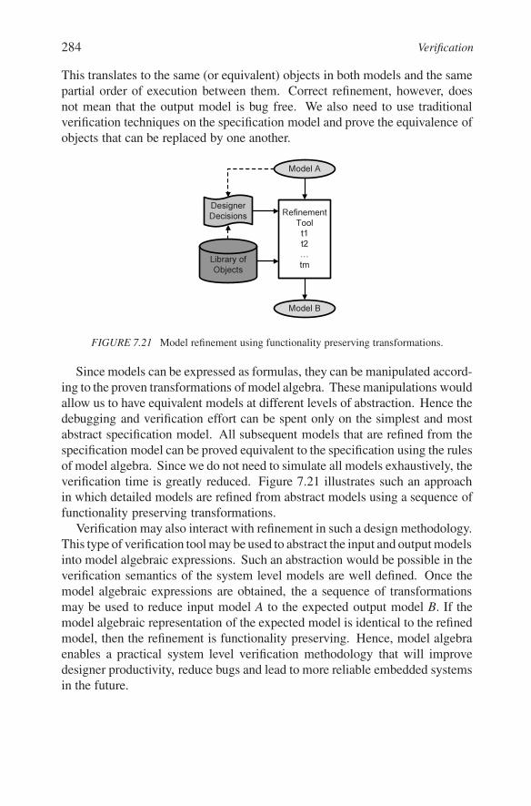
284 Verification

This translates to the same (or equivalent) objects in both models and the samepartial order of execution between them. Correct refinement, however, doesnot mean that the output model is bug free. We also need to use traditionalverification techniques on the specification model and prove the equivalence ofobjects that can be replaced by one another.

RefinementT o o lt1t2…tm

M o d el A

M o d el B

D es ig nerD ec is io ns

L ib r a r y o fO b j ec ts

FIGURE 7.21 Model refinement using functionality preserving transformations.

Since models can be expressed as formulas, they can be manipulated accord-ing to the proven transformations of model algebra. These manipulations wouldallow us to have equivalent models at different levels of abstraction. Hence thedebugging and verification effort can be spent only on the simplest and mostabstract specification model. All subsequent models that are refined from thespecification model can be proved equivalent to the specification using the rulesof model algebra. Since we do not need to simulate all models exhaustively, theverification time is greatly reduced. Figure 7.21 illustrates such an approachin which detailed models are refined from abstract models using a sequence offunctionality preserving transformations.

Verification may also interact with refinement in such a design methodology.This type of verification tool may be used to abstract the input and output modelsinto model algebraic expressions. Such an abstraction would be possible in theverification semantics of the system level models are well defined. Once themodel algebraic expressions are obtained, the a sequence of transformationsmay be used to reduce input model A to the expected output model B. If themodel algebraic representation of the expected model is identical to the refinedmodel, then the refinement is functionality preserving. Hence, model algebraenables a practical system level verification methodology that will improvedesigner productivity, reduce bugs and lead to more reliable embedded systemsin the future.

Summary 285

7.5 SUMMARYWe have looked at several verification techniques ranging from simulation

based methods to formal verification techniques. We also offered a comparativeanalysis of the various techniques and projected the future trend for systemlevel verification. As the size and complexity of designs increase, traditionaltechniques might not be able to keep pace. A system design methodology withwell defined model semantics may be a possible solution to the problem.

New challenges to the verification of embedded systems result from thegrowth in size and complexity of designs. Individually verified componentsdo not work together due to interface issues. Also the sheer size of designsmakes cycle accurate modeling and exhaustive simulation too expensive andtime consuming. To answer this challenge, we must develop a comprehen-sive and formal system level design methodology which will require formalsemantics for system level models. Furthermore, we must define methods forfunctionality preserving refinement of models from one abstraction level to thenext. As a result, traditional simulation based verification methods can still beused for system specification model while correct refinements will avoid theneed to simulate lower level cycle accurate models.

Specifying the design at a higher level of abstraction would also make tra-ditional simulation and debugging feasible because of the smaller model size.Well defined model semantics would make it possible to define and prove correcttransformations for automatic model refinement. Therefore, model formaliza-tion would make complete system verification much faster.