ELSEVIER COMPUTER NETWORKS 1 Efﬁcient eNB …wangyc/publications/journals/j024...Efﬁcient eNB...

ELSEVIER COMPUTER NETWORKS 1

Efficient eNB Deployment Strategy forHeterogeneous Cells in 4G LTE Systems

You-Chiun Wang and Chien-An Chuang

Abstract—Base station deployment is an important issue in cellular communication systems because it determines the cost to construct and

maintain a system and also the service quality to users. Conventional 2G and 3G systems assume that base stations are identical in the

sense that they have the similar coverage range. For 4G systems, LTE introduces the concept of heterogeneous base stations (also called

eNBs), which supports different sizes of coverage range. Given the user distribution and demands in a service area, the problem of deploying

heterogeneous eNBs is NP-hard. Therefore, we propose a four-stage eNB deployment strategy to efficiently solve the problem. Our strategy

first employs a geometric approach to provide the basic coverage to the service area. Then, it adaptively adjusts the cell range to satisfy

the user demands under the power and bandwidth constraints on each eNB. Simulation results verify that the proposed strategy not only

significantly saves the system cost, but also reduces the power consumption while balances the traffic loads of eNBs.

Index Terms—base station deployment, cell planning, heterogeneous network (HetNet), long term evolution (LTE), network management.

✦

1 INTRODUCTION

THE market of intelligent, hand-held communication de-vices such as mobile phones and tablet computers keeps

growing year by year. Except for the basic voice communi-cation, various wireless multimedia services with large band-width demand such as video streaming and teleconference ser-vices should be also supported by network operators. To fol-low this trend, ITU (International Telecommunication Union)defines IMT-A (International Mobile Telecommunications–Advanced) requirements for the current 4G communicationsystems [1]. Specifically, the target peak data rate (for totalusers) is 1 Gbps in the downlink and 500 Mbps in the uplink.Therefore, 3GPP (the third Generation Partnership Project)specifies long term evolution (LTE) and its advanced version,LTE-A, in order to meet the above IMT-A requirements [2].

For a cellular communication system, one critical issue is todetermine the locations of base stations (BSs), also known asBS deployment, so as to provide the maximum service coveragewith the minimum system cost. Existing 2G and 3G systemsusually consider BSs with similar hardware characteristicssuch as antennas and power levels. A network operator mayfirst predict where BSs should be located in theory or by sim-ulations so that not only the service coverage is increased butalso the interference between adjacent cells is reduced. Thus,BSs are often planned to be deployed in a regular fashion [3].Then, BSs are practically deployed wherever the operator canacquire rights to purchase and install sites. However, becauseall cells have the similar coverage range, the above deploymentmay not work well when users request large traffic demandsor some of them congregate in certain small regions (calledhotspots, such as coffee shops or airports) [4].

In LTE, a BS is also called an E-UTRAN NodeB (or eNBshortly). Depending on their coverage range, LTE definesfour types of eNBs (from large range to small range): macro-cell, micro-cell, pico-cell, and femto-cell eNBs. Only femto-celleNBs can be user-installed, whereas other eNBs are operator-

The authors are with the Department of Computer Science and Engineering,National Sun Yat-sen University, Kaohsiung, 80424, Taiwan.E-mail: [email protected]; [email protected]

TABLE 1: Comparison on LTE eNBs.eNB transmission power cell size users supported

macro-cell 20 W – 160 W > 1 km > micro-cellmicro-cell 2 W – 20 W 250 m – 1 km > pico-cellpico-cell 250 mW – 2 W 100 m – 300 m 32

femto-cell 10 mW – 200 mW 10 m – 50 m 8

[Unit] m: meter, km: kilometer, W: watt, mW: milliwatt[Notice] The typical transmission power of a macro-cell eNB is 40 W.

installed. Table 1 compares these four types of eNBs [5], [6].By allowing different types of eNBs to coexist in the same ser-vice area, LTE introduces the concept of heterogeneous network(HetNet) to address the above large user-demand and hotspotissues. In particular, macro-cell eNBs serve as the backboneto provide signal coverage in large geographic regions. Then,micro-cell and pico-cell eNBs can provide service to hotspotsor fill those ‘uncovered holes’ left by macro-cells. Finally, userscan install their own femto-cell eNBs to improve the signalquality.

The eNB deployment issue in LTE HetNets is also ad-dressed in the literature, but most of relevant research dis-cusses only the combination of large macro-cell and smallfemto-cell (or pico-cell) eNBs. This motivates us to study theeNB deployment with the minimum cost (EDMC) problem, wherethree types of operator-installed eNBs are considered (that is,macro-cell, micro-cell, and pico-cell eNBs). Given the distribu-tion of LTE user equipments (UEs) and their traffic demands,the EDMC problem asks how to deploy different eNBs tomeet the demands of all UEs such that the total system cost isminimized. The problem is NP-hard, so we develop an efficientfour-stage strategy. Our idea is to first use large cells to providebasic coverage to every UE. Then, for each cell, our strategychecks whether the eNB has sufficient power and bandwidthresource to support all UEs in the cell. If not, the cell range isshrunk accordingly. Finally, small cells are added to strengthenthe network deployment.

The contributions of this paper are threefold. First, theproposed EDMC problem considers all types of operator-installed eNBs, whereas many research efforts disregard micro-cell eNBs. Our EDMC solution thus helps support more flex-

2 ELSEVIER COMPUTER NETWORKS

ible network deployment. In addition, we consider path loss,shadowing, multipath fading, and environmental noise, whichcan model LTE communication channels more realistically.Second, we develop an efficient eNB deployment strategy byconsidering not only the positions of UEs but also the powerand bandwidth constraints on each eNB to meet UEs’ trafficdemands. Furthermore, several research issues of our strategysuch as the fluctuations in UE density, impact of uplink trans-mission, and cell interference are also discussed in the paper.Third, we design four different scenarios of UE distributionsin the simulations to evaluate the performance of our eNBdeployment strategy. Experimental results demonstrate thatour strategy can significantly save the overall system cost,reduce the power consumption of macro-cell eNBs, and dealout the load of each macro-cell eNB to its nearby small-celleNBs.

The rest of this paper is organized as follows. The nextsection discusses the related work. Section 3 first addressesthe eNB parameters and the fading and noise models usedto describe an LTE communication channel. Then, the sectionformally defines the EDMC problem. Section 4 presents oureNB deployment strategy to the EDMC problem and Section 5investigates some research issues in the proposed strategy.Experimental results are shown in Section 6. Finally, we givethe conclusion and future work in Section 7.

2 RELATED WORK

BS deployment has been widely discussed in 2G and 3G com-munication systems. For 2G systems, many research efforts[7]–[10] consider two-phase BS deployment. In phase 1, theyselect a set of candidate locations to place macro-cell BSsin order to meet the given capacity demand such that thesystem cost can be reduced. Then, phase 2 aims at allocatingfrequency channels to BSs such that the interference betweentwo adjacent cells can be eliminated while user QoS (qualityof service) can be satisfied. On the other hand, 3G systemsdo not require the above phase 2 since all BSs share the samefrequency spectrum. Therefore, 3G BS deployment [11]–[14]focuses on selecting the locations of BSs and adjusting theirtransmission power, with the consideration of cell interference.However, these studies only consider identical macro-cell BSsand thus their results may not be directly applied to wirelessHetNets. Ting et al. [15] propose a multi-objective variable-length genetic algorithm to address BS deployment in a wire-less HetNet containing both WiMAX and WiFi BSs, where thegoal is to maximize the network coverage while minimizingthe system cost. However, only two types of BSs are consideredand the BS planning model aims at the map instead of the userdistribution. The work of [16] proposes a budgeted cell planningproblem for cellular networks with small cells, and its objectiveis to maximize the number of traffic demand nodes whoserequired rates are fully satisfied under the budget constraint.The problem is proven to be NP-hard and an approximationalgorithm which yields an (e− 1)/2e fraction of the optimumis developed. Obviously, [16] has different objective with ourwork.

Several research efforts also investigate the LTE eNB de-ployment issue. By measuring the commercial GSM (GlobalSystem for Mobile Communications) live traffic to capture thespatial distribution of UEs, [17] can assess LTE downlink inter-cell interference and thus determine where to deploy macro-cell eNBs. However, it does not consider LTE HetNets. Both

[18] and [19] discuss how to efficiently add femto-cell eNBsin existing LTE macro-cells in order to improve the servicecoverage and network capacity. As mentioned earlier, femto-cell eNB are usually user-installed for private usage. Somestudies consider LTE HetNets with the coexistence of macro-cells and pico-cells. Specifically, the work of [20] determinesthe location, transmission power, and antenna tilt of eachpico-cell eNB with the help of CRE (cell range expansion)and TDM-ICIC (time domain multiplexing inter-cell interferencecoordination) techniques, which can balance macro-cell eNBs’loads and mitigate their interference, respectively. Barbera etal. [3] evaluate the effect of different pico-cell eNB deploymentand user mobility patterns on UE handover between LTEcells. Given the deployment of macro-cell and pico-cell eNBs,[21] seeks to ‘switch off’ some macro-cell eNBs to save theoverall energy. In this case, the nearby pico-cell eNBs will beresponsible for serving UEs so that there is no loss of networkcapacity. Apparently, these studies have different objectiveswith our EDMC problem. Zhao et al. [22], [23] consider theminimum-cost cell planning problem in an LTE HetNet, whichasks how to select a subset of candidate eNB sites (includingmacro-cell and pico-cell eNBs) in order to minimize the overalldeployment cost and satisfy the rate requirements of all UEs.The problem is NP-hard and they thus develop an O(logR)-approximation solution, where R is the maximum achievablecapacity of eNBs. Since the EDMC problem considers notonly macro-cells and pico-cells but also micro-cells, it is moredifficult than the above problem. Thus, the EDMC problem isNP-hard and we will propose an efficient eNB deploymentstrategy based on the distribution of UEs and their trafficdemands.

3 SYSTEM MODEL

In this section, we first present the parameters of eNBs usedin our deployment strategy. Then, we define the fading effectand noise to model an LTE communication channel and finallyformulate the EDMC problem.

3.1 eNB Parameters

We aim at the deployment of operator-installed eNBs in theservice area. Let Pmacro, Pmicro, and Ppico be the typical trans-mission power of a macro-cell, micro-cell, and pico-cell eNB,respectively. According to the transmission power, we canestimate the communication range of a macro-cell, micro-cell,and pico-cell eNB (respectively denoted by Rmacro, Rmicro,and Rpico). Apparently, higher transmission power implieslarger communication range (and thus a larger cell size). FromTable 1, we can obtain that Pmacro ≥ Pmicro ≥ Ppico andtherefore Rmacro ≥ Rmicro ≥ Rpico.

Although the communication range is tightly coupled withthe transmission power, we still separately define these twoparameters due to two reasons. First, both transmission powerand communication range are two fundamental eNB charac-teristics, where some eNB manufacturers also indicate thesetwo parameters in their products [6], [24]. (Table 1 also liststhe common transmission power and communication rangeof different LTE eNBs.) Second, separately defining transmis-sion power and communication range can help facilitate thedeployment process. In particular, we can easily ‘filter’ outthose UEs outside a cell by using the communication range.Then, each eNB can examine only the UEs inside its cell and

EFFICIENT ENB DEPLOYMENT STRATEGY FOR HETEROGENEOUS CELLS IN 4G LTE SYSTEMS 3

determine whether it has sufficient power to serve these UEs.In this way, the eNB does not need to examine every UE in theservice area.

On the other hand, let us denote by BDLmacro, BDL

micro, andBDL

pico the total downlink bandwidth supported by a macro-cell,micro-cell, and pico-cell eNB, respectively. These bandwidthparameters depend on the component carriers possessed by aneNB. The LTE standard allows a component carrier to havethe bandwidth of 1.4 MHz, 3 MHz, 5 MHz, 10 MHz, 15 MHz,and 20 MHz. Based on the operating frequency band of aneNB1, we can obtain its component carriers and thus estimatethe corresponding bandwidth. In addition, we define the costto install and maintain a macro-cell, micro-cell, and pico-celleNB by the notations Cmacro, Cmicro, and Cpico, respectively.According to [25], it is common that Cmacro > Cmicro > Cpico.

3.2 Fading and Noise Models

Generally speaking, a transmission signal will be affected bythree major types of fading: path loss, slow fading (also calledshadowing fading), and fast fading (also called multipath fading).These fading effects are important to model a wireless channel.Specifically, path loss is the power attenuation of a signal in thepropagation environment when it travels from the transmitterto the receiver. According to the LTE standard (Release 9)[26], we employ the log-distance model to estimate path loss.In particular, the path-loss effect of a macro-cell is calculatedby

PLmacro = 128.1 + 37.6 log10(r), (1)

where r is the distance between a UE and the eNB (in kilome-ters). For both micro-cells and pico-cells, the path-loss effect ismeasured by

PLsmall = 140.7 + 36.7 log10(r). (2)

On the other hand, slow fading is the obstruction encoun-tered by a signal when some objects (such as buildings or trees)block its transmission path. It will result in random variationin the signal’s amplitude and thus cannot be simply modeledby path loss. Therefore, we adopt the popular log-normal shad-owing model [27] to estimate slow fading. Specifically, let usdenote by S the random variable of the ratio of the powertransmitted to the power received in decibel (dB) scale, wherethe received signal power is attenuated by slow fading. Then,the probability distribution of S can be expressed by

p(S) = 1√2πσ

exp

(−(S − µ)2

2σ2

)

, (3)

where µ and σ are the mean and standard deviation of S indB, respectively. The LTE standard suggests setting µ = 0 dB(that is, zero mean), and σ = 10 dB and 6 dB for a macro-celland micro-cell/pico-cell eNB, respectively.

Fast fading is caused by the reception of a signal at thereceiver from more than one path. Jakes fading model [28]and its variations are widely used to evaluate such an effect.They consider a moving UE that receives k rays with equalsignal strength. Each ray i arrives at an angle of αi = 2πi/kand encounters a Doppler shift of ωi = ωmax cos(αi), whereωmax = 2πfv/c is the maximum Doppler shift which will be

1. ITU totally defines 44 frequency bands for LTE operation. Eachnetwork operator has to apply for some of them (usually two to threebands) before operating. Therefore, which bands are operated by an eNBis actually known in advance.

encountered at receiver speed of v, carrier frequency f , andspeed of light c. Then, the signal waveform received by the UEcan be expressed by a function of time t:

g(t) =Υ

(

1√2(cos(α) + j sin(α)) · cos(ωmaxt+ θ0)+

N∑

i=1

(cos(βi) + j sin(βi)) · cos(ωit+ θi)

)

, (4)

where Υ is a normalization constant and N = (k/2− 1)/2. InEq. (4), the variables j, α, βi, and θi are the model parameters.

Except for the fading effects, the thermal noise in the en-vironment will also affect the transmission signal. To simulatesuch noise, we employ the additive white Gaussian noise (AWGN)model [29] as suggested by the LTE standard, where the powerspectral density of AWGN is set to -174 dBm/Hz (decibel-milliwatt per hertz).

3.3 The EDMC Problem

Let E be the set of all possible sites on which the networkoperator acquires rights to deploy eNBs in the service area. The

EDMC problem seeks to select a subset of E to deploy eNBswith the minimum cost so as to satisfy the traffic demands of a

set of UEs U , where the total amount of power and bandwidthof each eNB allocated to its UEs cannot exceed the giventhresholds (defined in Section 3.1). Specifically, let ei denotethe selection variable of an eNBi, where

ei =

{

1 eNBi is selected for deployment,0 otherwise,

∀i ∈ E.

Then, the EDMC problem can be formulated as follows:

minei,pi,j ,bi,j

∑

i∈E

eiCi, Ci ∈ {Cmacro, Cmicro, Cpico} (5)

such that∑

uj∈U

bDLi,j ≤ eiB

DLi ,

∀i ∈ E, BDLi ∈ {BDL

macro, BDLmicro, B

DLpico} (6)

∑

uj∈U

pi,j ≤ eiPi,

∀i ∈ E, Pi ∈ {Pmacro, Pmicro, Ppico} (7)∑

i∈E

rDLi,j ≥ rDL

j , ∀uj ∈ U , (8)

bDLi,j ≥ 0, pi,j ≥ 0, ∀i ∈ E, uj ∈ U , (9)

under the channel constraints defined in Section 3.2, where Ci,BDL

i , and Pi are respectively the cost, downlink bandwidth,and transmission power of eNBi (depending on its type); pi,j ,bDLi,j , rDL

i,j are respectively the downlink power, bandwidth,

and data rate that eNBi allocates to a UE uj ; rDLj is the

expected downlink traffic demand of uj . Here, Eq. (5) isthe objective function, which wants to minimize the overallsystem cost. Eqs. (6) and 7 respectively indicate that the totalbandwidth and power of eNBi allocated to all UEs in its cellcannot exceed the thresholds BDL

i and Pi. Eq. (8) means thatthe deployment of eNBs should satisfy the expected downlinktraffic demand of each UE. Eq. (9) shows that the allocation ofpower and bandwidth for UEs is non-negative.


UE locations

Modified AHC scheme

Weighted K-means

approach

Kmacro & Kmicro

Macro-cells & micro-cells

Does the eNB

have enough

resource?

Check the next eNB.

Yes

Adjust the cell range

until the eNB can

support all UEs.

No

Have checked

all eNBs?

No

Yes

Is there any

uncovered UE?

YesUse the MGDC scheme

to find pico-cells to

cover such UEs.

No

UE demands

Finish

Stage 1: estimating the

number of eNBs

Stage 2: preliminary

deployment of large cells

Stage 3: range adjustment

in each cell

Stage 4: adding

pico-cells

Fro

m g

eo

me

tric

pers

pe

cti

ve

Fro

m r

eso

urc

e’s

pers

pe

cti

ve

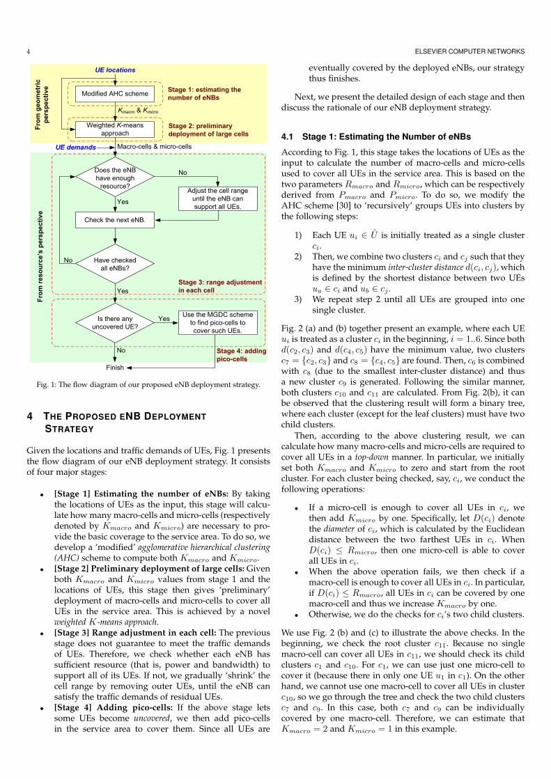
Fig. 1: The flow diagram of our proposed eNB deployment strategy.

4 THE PROPOSED ENB DEPLOYMENT

STRATEGY

Given the locations and traffic demands of UEs, Fig. 1 presentsthe flow diagram of our eNB deployment strategy. It consistsof four major stages:

• [Stage 1] Estimating the number of eNBs: By takingthe locations of UEs as the input, this stage will calcu-late how many macro-cells and micro-cells (respectivelydenoted by Kmacro and Kmicro) are necessary to pro-vide the basic coverage to the service area. To do so, wedevelop a ‘modified’ agglomerative hierarchical clustering(AHC) scheme to compute both Kmacro and Kmicro.

• [Stage 2] Preliminary deployment of large cells: Givenboth Kmacro and Kmicro values from stage 1 and thelocations of UEs, this stage then gives ‘preliminary’deployment of macro-cells and micro-cells to cover allUEs in the service area. This is achieved by a novelweighted K-means approach.

• [Stage 3] Range adjustment in each cell: The previousstage does not guarantee to meet the traffic demandsof UEs. Therefore, we check whether each eNB hassufficient resource (that is, power and bandwidth) tosupport all of its UEs. If not, we gradually ‘shrink’ thecell range by removing outer UEs, until the eNB cansatisfy the traffic demands of residual UEs.

• [Stage 4] Adding pico-cells: If the above stage letssome UEs become uncovered, we then add pico-cellsin the service area to cover them. Since all UEs are

eventually covered by the deployed eNBs, our strategythus finishes.

Next, we present the detailed design of each stage and thendiscuss the rationale of our eNB deployment strategy.

4.1 Stage 1: Estimating the Number of eNBs

According to Fig. 1, this stage takes the locations of UEs as theinput to calculate the number of macro-cells and micro-cellsused to cover all UEs in the service area. This is based on thetwo parameters Rmacro and Rmicro, which can be respectivelyderived from Pmacro and Pmicro. To do so, we modify theAHC scheme [30] to ‘recursively’ groups UEs into clusters bythe following steps:

1) Each UE ui ∈ U is initially treated as a single clusterci.

2) Then, we combine two clusters ci and cj such that theyhave the minimum inter-cluster distance d(ci, cj), whichis defined by the shortest distance between two UEsua ∈ ci and ub ∈ cj .

3) We repeat step 2 until all UEs are grouped into onesingle cluster.

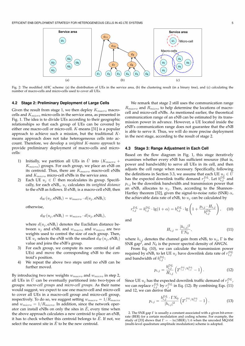
Fig. 2 (a) and (b) together present an example, where each UEui is treated as a cluster ci in the beginning, i = 1..6. Since bothd(c2, c3) and d(c4, c5) have the minimum value, two clustersc7 = {c2, c3} and c8 = {c4, c5} are found. Then, c6 is combinedwith c8 (due to the smallest inter-cluster distance) and thusa new cluster c9 is generated. Following the similar manner,both clusters c10 and c11 are calculated. From Fig. 2(b), it canbe observed that the clustering result will form a binary tree,where each cluster (except for the leaf clusters) must have twochild clusters.

Then, according to the above clustering result, we cancalculate how many macro-cells and micro-cells are required tocover all UEs in a top-down manner. In particular, we initiallyset both Kmacro and Kmicro to zero and start from the rootcluster. For each cluster being checked, say, ci, we conduct thefollowing operations:

• If a micro-cell is enough to cover all UEs in ci, wethen add Kmicro by one. Specifically, let D(ci) denotethe diameter of ci, which is calculated by the Euclideandistance between the two farthest UEs in ci. WhenD(ci) ≤ Rmicro, then one micro-cell is able to coverall UEs in ci.

• When the above operation fails, we then check if amacro-cell is enough to cover all UEs in ci. In particular,if D(ci) ≤ Rmacro, all UEs in ci can be covered by onemacro-cell and thus we increase Kmacro by one.

• Otherwise, we do the checks for ci’s two child clusters.

We use Fig. 2 (b) and (c) to illustrate the above checks. In thebeginning, we check the root cluster c11. Because no singlemacro-cell can cover all UEs in c11, we should check its childclusters c1 and c10. For c1, we can use just one micro-cell tocover it (because there in only one UE u1 in c1). On the otherhand, we cannot use one macro-cell to cover all UEs in clusterc10, so we go through the tree and check the two child clustersc7 and c9. In this case, both c7 and c9 can be individuallycovered by one macro-cell. Therefore, we can estimate thatKmacro = 2 and Kmicro = 1 in this example.


Service area

u1

u2

u3

u4

u5

u6

(a)

c1 c2 c3 c4 c5 c6

c7 c8

c9

c10

c11

(b)

Service area

u1

u2

u3

u4

u5

u6

Micro-cell

Macro-cells

(c)

Fig. 2: The modified AHC scheme: (a) the distribution of UEs in the service area, (b) the clustering result (in a binary tree), and (c) calculating thenumber of macro-cells and micro-cells used to cover all UEs.

4.2 Stage 2: Preliminary Deployment of Large Cells

Given the result from stage 1, we then deploy Kmacro macro-cells and Kmicro micro-cells in the service area, as presented inFig. 1. The idea is to divide UEs according to their geographicrelationships so that each group of UEs can be covered byeither one macro-cell or micro-cell. K-means [31] is a popularapproach to achieve such a mission, but the traditional K-means approach does not take heterogeneous cells into ac-count. Therefore, we develop a weighted K-means approach toprovide preliminary deployment of macro-cells and micro-cells:

1) Initially, we partition all UEs in U into (Kmacro +Kmicro) groups. For each group, we place an eNB onits centroid. Thus, there are Kmacro macro-cell eNBsand Kmicro micro-cell eNBs in the service area.

2) Each UE uj ∈ U then recalculates its group. Specifi-cally, for each eNBi, uj calculates its weighted distanceto the eNB as follows. If eNBi is a macro-cell eNB, then

dW (uj , eNBi) = wmacro · d(uj , eNBi);

otherwise,

dW (uj , eNBi) = wmicro · d(uj , eNBi),

where d(uj , eNBi) denotes the Euclidian distance be-tween uj and eNBi and wmacro and wmicro are twoweights used to control the size of each group. Then,UE uj selects the eNB with the smallest dW (uj , eNBi)value and joins the eNB’s group.

3) For each group, we compute its new centroid (of allUEs) and move the corresponding eNB to the cen-troid’s position.

4) We repeat the above two steps until no eNB can befurther moved.

By introducing two new weights wmacro and wmicro in step 2,

all UEs in U can be eventually partitioned into two-types ofgroups: macro-cell groups and micro-cell groups. As their namewould suggest, we expect to use one macro-cell and micro-cellto cover all UEs in a macro-cell group and micro-cell group,respectively. To do so, we suggest setting wmacro = 1/Rmacro

and wmicro = 1/Rmicro. In addition, since the network oper-

ator can install eNBs on only the sites in E, every time whenthe above approach calculates a new centroid to place an eNB,

it has to check whether this centroid belongs to E. If not, we

select the nearest site in E to be the new centroid.

We remark that stage 2 still uses the communication rangeRmacro and Rmicro to help determine the locations of macro-cell and micro-cell eNBs. As mentioned earlier, the theoreticalcommunication range of an eNB can be estimated by its trans-mission power in advance. However, a UE located inside theeNB’s communication range does not guarantee that the eNBis able to serve it. Thus, we will do more precise deploymentin the next stage, according to the result of stage 2.

4.3 Stage 3: Range Adjustment in Each Cell

Based on the flow diagram in Fig. 1, this stage iterativelyexamines whether every eNB has sufficient resource (that is,power and bandwidth) to serve all UEs in its cell, and thenadjusts the cell range when necessary. Specifically, following

the definitions in Section 3.3, we assume that each UE uj ∈ Uhas the expected downlink traffic demand rDL

j . Let bDLi,j and

pi,j be the downlink bandwidth and transmission power thatan eNBi allocates to uj . Then, according to the Shannon-Hartley theorem [32], given the signal-to-noise ratio (SNR) α,the achievable data rate of eNBi to uj can be calculated by

rDLi,j = bDL

i,j · lg(1 + α) = bDLi,j · lg

(

1 +pi,j ·Hi,j

bDLi,j

)

, (10)

and

Hi,j =|hi,j |2ΓN0

, (11)

where hi,j denotes the channel gain from eNBi to uj , Γ is theSNR gap2, and N0 is the power spectral density of AWGN.

From Eq. (10), we can calculate the transmission powerrequired by eNBi to let UE uj have downlink data rate of rDL

i,j

and bandwidth of bDLi,j :

pi,j =bDLi,j

Hi,j

(

2rDLi,j /bDL

i,j − 1)

. (12)

Since UE uj has the expected downlink traffic demand of rDLj ,

we can replace rDLi,j by rDL

j in Eq. (12). By combining Eqs. (11)and 12, we can derive that

pi,j =bDLi,j · ΓN0

|hi,j |2(

2rDLj /bDL

i,j − 1)

. (13)

2. The SNR gap Γ is usually a constant associated with a given bit-error-rate (BER) for a certain modulation and coding scheme. For example, thestudy of [33] shows that Γ = − ln(5BER)/1.6 when the uncoded MQAM(multi-level quadrature amplitude modulation) scheme is adopted.


Macro-cell

eNB

uj

(a)

Micro-cell

eNB

uj

(b)

Fig. 3: An example of the second extension in stage 3: (a) the originalmacro-cell and (b) replacing the macro-cell with a micro-cell by discardingUE uj .

Therefore, each eNBi can use Eq. (13) to determine whether

it can support all UEs in its cell. Specifically, let Ui ⊆ Udenote the set of UEs in eNBi’s cell (calculated by stage2). Suppose that Pi and BDL

i are the overall transmissionpower and downlink bandwidth of eNBi, respectively. Ob-viously, when eNBi is a macro-cell eNB, then Pi = Pmacro

and BDLi = BDL

macro. On the other hand, Pi = Pmicro andBDL

i = BDLmicro if eNBi is a micro-cell eNB. Then, eNBi can do

the following check:∑

uj∈Ui

pi,j ≤ Pi, (14)

under the constraint of∑

uj∈Ui

bDLi,j ≤ BDL

i . (15)

Notice that pi,j and bDLi,j are not fixed in the above calculation.

Instead, they are computed by eNBi according to the expecteddownlink traffic demand rDL

j . However, if eNBi cannot find

a feasible solution of pi,j and bDLi,j to satisfy Eqs. (14) and

15, it means that eNBi currently has no sufficient power orbandwidth resource to meet the downlink traffic demands ofall its UEs. In this case, eNBi has to give up some UEs in thecell. Specifically, starting from the farthest UE, say, uj , eNBi

iteratively marks uj as uncovered and removes the UE from itscell, until the above two equations become satisfied. Therefore,we can make sure that every eNB can support all UEs in itscell.

We remark that two extensions can help further improvestage 3. First, when a UE is marked as uncovered by itsoriginal eNB, the UE can check whether other nearby eNBshave sufficient power and bandwidth resource to serve it. Ifso, the UE can join the nearest one of such eNBs. Second, if amacro-cell eNB finds that it can use transmission power Pmicro

and downlink bandwidth BDLmicro to serve all UEs in the current

cell, then we can replace the eNB by a micro-cell eNB. Thisextension may occur when a macro-cell eNB discards somefarther UEs and the residual UEs are close to it. Fig. 3 showsan example. When the macro-cell eNB discards the farthest UEuj , then it can be replaced by a micro-cell eNB to serve theresidual UEs.

4.4 Stage 4: Adding Pico-cells

After the range adjustment in stage 3, there could remain someUEs not covered by any large cell. These UEs are usually

u1

u2

u3

u4

u5

Rpico

2Rpico< 2Rpico

Fig. 4: Using the MGDC scheme to find the locations of pico-cells.

isolated from others, or locate near the boundary between twocells. Obviously, it is wasteful if we simply deploy macro-cellsor micro-cells to cover such UEs, because each cell can onlyserve a small number of UEs. Therefore, we suggest usingpico-cell eNBs to deal with this situation, as described in Fig. 1.

Specifically, let UR ⊂ U denote the set of UEs not covered byany cell after stage 3. We then adopt the modified geometric diskcover (MGDC) scheme in [34] to find possible sites to deploypico-cells, which involves the three rules:

1) If two UEs ui and uj in UR have a distance d(ui, uj) <2Rpico, we deploy two pico-cells such that their cir-cumferences intersect at ui and uj .

2) If two UEs ui and uj in UR have a distance d(ui, uj) =2Rpico, we deploy one pico-cell such that it circumfer-ence passes both ui and uj .

3) If a UE uk ∈ UR is isolated, which means that itsdistance to the closest UE is larger than 2Rpico, wedeploy a pico-cell whose center is on uk.

Fig. 4 gives three examples. Since we have to check each

pair of UEs in UR, the maximum number of pico-cells found by

the MGDC scheme will be 2C|UR|2 , where C

|UR|2 = |UR|!

2!(|UR|−2)!

is the combination of selecting two UEs from the set UR. In

practice, we require at most |UR| pico-cells to cover these UEs.Therefore, among all pico-cells found by the MGDC scheme,

we select the pico-cell whose center belongs to E (that is, thenetwork operator can deploy a pico-cell eNB on that location)

and it can cover the maximum number of UEs in UR. Then, weuse the scheme in Section 4.3 again to determine the UEs thatcan be served by the corresponding pico-cell eNB (to satisfyEqs. (14) and 15 where Pi = Ppico and BDL

i = BDLpico). The

above iteration is repeated until all UEs in UR are served bypico-cell eNBs.

4.5 Rationale of the eNB Deployment Strategy

Given the transmission power of an eNB, we can easily de-rive its theoretical communication range. Besides, some eNBmanufacturers also give both the parameters of transmissionpower and communication range in their products. Therefore,our eNB deployment strategy takes advantage of these twoparameters and can be roughly divided into two parts, asshown in Fig. 1. In the first part (that is, stages 1 and 2),we seek to determine the locations of eNBs from a geometricperspective so as to provide the preliminary network deploy-ment. Specifically, our objective is to identify where most ofUEs congregate so that we can effectively employ large cellssuch as macro-cells and micro-cells to cover them. However,a UE that can be covered by an eNB does not imply that theeNB can provide service to meet the traffic demand of that UE.Therefore, the second part of our strategy (that is, stages 3 and4) attempts to determine the actual service range of each eNB


from a resource’s perspective. In particular, we carefully checkif every eNB has sufficient amount of power and bandwidthto support all UEs in its cell, and adjust their cell range ifnecessary. Then, we would add small pico-cells to strengthenthe network deployment.

For the first part, K-means is a popular solution to groupUEs according to their relative geographic locations. However,the traditional K-means approach cannot be directly appliedto our EDMC problem because of two reasons: 1) The K-meansapproach requires the knowledge of K value in advance. 2)The K-means approach does not take the size of macro-cellsand micro-cells (that is, Rmacro and Rmicro) into consideration.To solve these two problems, we modify the AHC scheme instage 1 to estimate the number of macro-cells and micro-cellsrequired to cover all UEs (based on the Rmacro and Rmicro

values). Then, in stage 2, we introduce two weights wmacro

and wmicro to the K-means approach, so that UEs can bepartitioned into multiple groups such that the size of eachgroup could be constrained by either a macro-cell or micro-cellin substance. This is realized by setting wmacro = 1/Rmacro

and wmicro = 1/Rmicro (that is, the reciprocal of the commu-nication range of an eNB).

It is noteworthy that one may argue that the AHC schemehas already provided a clustering result to deploy macro-cellsand micro-cells, which makes the weighted K-means approachin stage 2 become redundant. However, stage 2 is necessaryto our eNB deployment strategy due to the following reason:The AHC scheme iteratively combines two clusters accordingto their inter-cluster distance. Unlike the weighted K-meansapproach, it does not take the congregation degree of UEs intoaccount. Therefore, a larger macro-cell could cover just fewUEs (if they are sparsely scattered) whereas a smaller micro-cell may have to cover a lot of UEs. Using the weighted K-means approach can alleviate the above situation by balancingUEs among different cells. Through the simulations in Sec-tion 6, we will also show that using the weighted K-meansapproach in stage 2 can significantly outperforms the case ofusing only the AHC scheme.

For the second part, we use the expected downlink trafficdemand rDL

j of each UE uj in stage 3 to estimate the amountof downlink bandwidth and power that its eNB has to allo-cate. However, the overall allocation of bandwidth and powercannot exceed the eNB’s thresholds BDL

macro (or BDLmicro) and

Pmacro (or Pmicro). In case an eNB does not have sufficientresource to satisfy the downlink traffic demands of all itsUEs, the eNB iteratively removes the farthest UE until theresidual UEs can be served. Since there is a high possibilitythat farther UEs will encounter worse channel quality (andlower SNR values), removing such UEs can help improve thenetwork throughput in a cell. We also discuss two extensionsin Section 4.3 to adaptively expand or shrink cell range soas to reduce the system cost. However, if there are still someUEs not covered by any cell, we finally add pico-cells in stage4 to serve them. Here, because a pico-cell has quite smallercommunication range (referring to Table 1), we only use themto strength the network deployment by serving the UEs thatare isolated from others or cannot be covered by large cells.Therefore, we can further save the system cost since pico-celleNBs have a lower price and maintenance cost as comparedwith large-cell eNBs.

5 DISCUSSIONS ON THE ENB DEPLOYMENT

STRATEGY

In this section, we investigate several research issues arisen inour eNB deployment strategy, including the fluctuations in UEdensity, impact of uplink transmission, and cell interference.

5.1 Fluctuations in UE Density

The EDMC problem considers that the locations of UEs aredeterministic and known in advance. In practice, the UEdensity will fluctuate over different times. For example, adowntown office area usually contains many UEs in work-days but may become almost empty during weekends. Suchfluctuations could be regular and even predictable. To accom-modate our eNB deployment strategy to the above situation,we suggest that the network operator should gather statisticsof UE distributions during different periods on each day ina week (for example, morning, afternoon, and night time of

one day). Let Uk denote the set of UEs observed in period

k and U =⋃

∀k Uk. Based on the information from U , thenetwork operator can plan to deploy all necessary eNBs inthe service area in order to react to the regular change of UEdensity. Specifically, When the UE density or traffic demandschange substantially, the network operator can employ oureNB deployment strategy to calculate the subset of eNBsthat should be kept operating to provide service. Then, otherunnecessary eNBs can be temporarily switched off to reducethe amount of energy consumption.

Sometimes, a service area may ordinarily contain few UEsbut is crowded with a large number of UEs in short term dueto special activities (for example, a singing concert). In thiscase, it is not economic for the network operator to deploy alot of eNBs in advance because the UE density will suddenlydecrease once the activity finishes. To deal with such situations,the network operator can use the set of UEs appearing inthe service area in ordinary time to calculate the locations todeploy backbone eNBs. Then, when many exterior UEs comeinto the service area, the network operator may adaptively add‘maneuverable’ eNBs such as mobile relay stations [35], [36] toserve these UEs. In this way, the network operator can dealwith the case when the UE density changes drastically andirregularly, because some eNBs could be dynamically movedto different locations to support various communication mis-sions.

The above two scenarios also demonstrate the benefit ofusing LTE HetNets. In particular, once the eNB deploymentfor an LTE HetNet is determined, the network operator canchoose to switch eNBs on/off to save energy or dispatchmaneuverable eNBs to meet high traffic demands. Therefore,it not only accommodates an LTE HetNet to the changedenvironment (for example, diverse UE density) but also helpsdecrease the cost of maintenance and operation.

5.2 Impact of Uplink Transmission

In stages 3 and 4 of our eNB deployment strategy, we employthe transmission power of an eNB (that is, Pmacro, Pmicro,and Ppico) to determine whether the eNB can support thetraffic demands of all UEs in its cell. However, the abovedetermination is from a ‘downlink’ perspective. Due to thepower limitation of UEs, it may not guarantee that each UEcan successfully transmit the uplink data to its eNB. To solvethis problem, we revise Eq. (13) to check if every eNB can


receive the uplink data from all of its UEs. Specifically, let PUE

denote the typical transmission power of UEs. From Eq. (13),we can derive that

bULi,j · (2rUL

j /bULi,j − 1) =

PUE · |hj,i|2ΓN0

(16)

Here, bULi,j is the bandwidth that eNBi allocates for UE uj to

transmit its uplink data, rULj is expected uplink traffic demand

of uj , and hj,i is the channel gain from uj to eNBi. In Eq. (16),we are given the parameters of PUE and rUL

j in advance.Besides, hj,i, Γ, and N0 are known environmental parameters.Therefore, we can calculate the necessary uplink bandwidthbULi,j that eNBi should reserve for uj . Then, for each eNBi, we

check whether∑

uj∈Ui

bULi,j ≤ BUL

i , (17)

where BULi ∈ {BUL

macro, BULmicro, B

ULpico} is the total uplink

bandwidth of an eNB (depending on its type) and Ui is theset of UEs served by eNBi. If Eq. (17) is violated, which meansthat some UEs may fail to send their uplink data, eNBi theniteratively removes the farthest UE in its cell, until Eq. (17)becomes satisfied.

5.3 Cell Interference

In Section 3.1, we mention that the communication range of aneNB can be estimated by its transmission power. It has beenpointed out in [37] that such estimation highly depends onthe path-loss fading. Therefore, given the transmission powerof an eNB, we can employ Eqs. (1) and 2 to calculate itscorresponding communication range, without caring aboutwhich component carriers assigned to that eNB. However,once the locations of eNBs are determined, the assignmentof component carriers becomes important. In particular, iftwo adjacent eNBs are assigned with the similar componentcarriers, they may cause interference between each other.Fortunately, LTE introduces the technology of ICIC (inter-cellinterference coordination) and eICIC (enhanced ICIC) to deal withthe above interference problem. ICIC allows eNBs to negoti-ate the usage of resource blocks through their X2 interfaces.Therefore, UEs near the cell edges are allocated with differentresource blocks to avoid interference. On the other hand,eICIC is developed for LTE HetNets, which employs differentnegotiation strategies for different types of eNBs. In addition,eICIC proposes the concept of almost blank subframe (ABS) toalleviate the interference to a small cell (such as pico-cells)from a large macro-cell. Due to the page limitation, we leavethe details of both ICIC and eICIC in [38].

6 EXPERIMENTAL RESULTS

In this section, we measure the performance of our eNBdeployment strategy by using MATLAB, which provides mod-ules to simulate LTE channels (for example, multipath fading).Table 2 lists our simulation parameters for eNBs. The typicaltransmission power of UEs PUE is set to 27 dBm (around500 mW). The expected uplink and downlink traffic demandsof UEs are randomly picked from rUL

j ∈ [0, 0.3]Mbps and

rDLj ∈ [0.1, 1.0]Mbps, respectively. Besides, we consider four

scenarios to model the distribution of UEs:

• Small-group scenario: There are 300 UEs placed in a12 km× 16 km service area. Most UEs congregate in the

TABLE 2: Simulation parameters for LTE eNBs.parameters macro-cell micro-cell pico-cellcell size 3 km 1 km 0.1 kmpower 46 dBm (40 W) 33 dBm (2 W) 24 dBm (0.25 W)bandwidth∗ 100 MHz 100 MHz 30 MHzcost [25] 397,800 Euros 42,200 Euros 12,400 Eurospath loss Eq. (1) Eq. (2) Eq. (2)slow fading µ = 0, σ = 10 dB µ = 0, σ = 6 dB µ = 0, σ = 6 dBcommon AWGN power density (N0): -174 dBm/Hzparameters Bit error rate (BER): 10−6

SNR gap (Γ): 7.6288∗The ratio of uplink to downlink bandwidth is 1:4.

middle part of the service area, as shown in Fig. 5(a). Inthis scenario, the network operator can deploy eNBs atany locations inside the service area.

• Large-group scenario: We consider a 20 km× 20 kmservice area over which 600 UEs are scattered follow-ing the normal distribution, as illustrated in Fig. 5(b).Similar to the above scenario, the network operator canfreely deploy eNBs in the service area.

• Multi-group scenario: Totally 1,800 UEs are placed in a30 km× 35 km service area and they can be roughly di-vided into five groups, as Fig. 5(c) presents. Again, thenetwork operator can choose any locations to deployeNBs.

• Downtown scenario: We take a part of the downtownarea in Kaohsiung City, Taiwan to be the service area,which is a square region whose wide is 18 km, as shownin Fig. 5(d). In this scenario, the network operator is

allowed to deploy eNBs only along streets (that is, Econtains all street subregions).

We compare our proposed eNB deployment strategy withthree methods:

• Macro-cell deployment (MCD) method: Like 2G and3G systems, this method deploys only macro-cell eNBs.We employ the rules in stage 3 to check whether everymacro-cell eNB can serve all UEs in its cell and addextra macro-cells to the service area when necessary.The MCD method is used as a baseline to observe thebenefit and flexibility of using LTE HetNets.

• AHC two-type-cell deployment (ATD) method: Weadopt the modified AHC scheme in stage 1 to clusterUEs into macro-cell and micro-cell groups. For eachgroup of UEs, we deploy the corresponding type ofeNB to provide service. Then, after shrinking the cellrange of eNBs (by stage 3), we add micro-cells to coverthose unserved UEs.

• Traditional K-means deployment (TKD) method: It issimilar to our eNB deployment strategy, but in stage3 we use the traditional K-means approach to helpdeploy eNBs. In addition, this method does not employthe two extensions proposed in stage 3.

Each experiment contains 100 simulations, where in eachsimulation we randomly generate the expected traffic de-mands of UEs (that is, rUL

j and rDLj ) to observe their effect. Ac-

cording to the locations of UEs (defined in the four scenarios)and their demands, each deployment method then determineswhere to install eNBs and calculates the amount of their powerconsumption. We then take the average of these 100 simulationresults in each experiment.


0

16

14

12

10

8

6

4

2

2 4 6 8 10 12

(a) small-group scenario

20

0

16

12

8

4

4 8 12 16 20

(b) large-group scenario

35

30

25

20

15

10

5

302520151050

(c) multi-group scenario

121086420 14 16 18

2

4

8

10

12

14

16

18

6

(d) downtown scenario

Fig. 5: Four scenarios to model the distribution of UEs.

6.1 System Cost

Using the four scenarios in Fig. 5, we first evaluate the systemcosts spent by the MCD, ATD, and TKD methods and oureNB deployment strategy, as shown in Fig. 6. Apparently, thesystem cost increases as the number of UEs grows because eacheNB has limited power and bandwidth resource to serve them.The MCD method considers only macro-cells, so it always re-sults in the highest system cost. On the contrary, by deployingdifferent types of eNBs in the service area, other three methodscan greatly reduce the overall system cost. From Fig. 6, we canobserve that the ATD and TKD methods use the same numberof macro-cell eNBs because they both employ the modifiedAHC scheme to calculate the required number of macro-celleNBs (that is, Kmacro). The ATD method needs slightly moremicro-cell eNBs than the TKD method since it employs extramicro-cell eNBs to cover those unserved UEs after shrinkingthe cell range of macro-cell eNBs. However, the TKD methodjust uses the traditional K-means approach to cluster UEs,which does not consider the difference between macro-cellsand micro-cells. Thus, it would require more pico-cells to coverthose unserved UEs and thus increases the system cost. On theother hand, by adopting the two extensions proposed in stage3, our eNB deployment strategy can further reduce macro-cellsdeployed in the service area. In this case, it suggests usingsmaller micro-cells and pico-cells to help cover the servicearea in order to save the overall system cost. On average, oureNB deployment strategy can save 48.07%, 21.59%, and 22.49%of the system cost compared with the MCD, ATD, and TKDmethods, respectively, in the four scenarios of UE distribution.

Both the large-group and downtown scenarios have the

same number of users (that is, 600 UEs). However, whencomparing Fig. 6(b) with Fig. 6(d), we can observe that alldeployment methods require more system costs in the down-town scenario than that in the large-group scenario. There aretwo reasons to cause such phenomena. First, the large-groupscenario lets UEs be scattered over the service area by usingthe normal distribution. In this case, we can deploy macro-cells near the central part of the area to cover a larger numberof UEs. On the other hand, UEs arbitrarily appear along thestreets in the downtown scenario, so it is not easy to deployjust few macro-cells to cover most of UEs. Second, the networkoperator can freely deploy eNBs in the large-group scenariobut is allowed to install eNBs only on the street subregions in

the downtown scenario. The constraint of E in the downtownscenario would force the network operator to use more eNBsto serve UEs as it cannot install eNBs on those ‘good’ locations

not in E.

Recall that we have discussed the two possible solutionsto the problem of fluctuations in UE density in Section 5.1.Suppose that the network operator knows that the distributionof UEs will alternate between the small-group scenario andthe large-group scenario in Fig. 5. Then, we can take theunion of both scenarios to calculate the locations to installall necessary eNBs. When the distribution of UEs changefrom one scenario to another scenario, the network operatorcan adaptively switch off unnecessary eNBs to react to thedistribution change of UEs. On the other hand, suppose thatthe distribution of UEs in a service area follows the large-groupscenario in ordinary time but may evolve to the multi-groupscenario due to some special activity. In this case, the network


0

20

40

60

80

100

120

140

160

MCD ATD TKD ours

syste

mcost

(100,0

00

Euro

s)

pico-cell

micro-cell

macro-cell


0

20

40

60

80

100

120

140

160

MCD ATD TKD ours

syste

mcost

(100,0

00

Euro

s)

pico-cell

micro-cell

macro-cell


0

20

40

60

80

100

120

140

160

MCD ATD TKD ours

syste

mcost

(100,0

00

Euro

s)

pico-cell

micro-cell

macro-cell


0

20

40

60

80

100

120

140

160

MCD ATD TKD ours

syste

mcost

(100,0

00

Euro

s)

pico-cell

micro-cell

macro-cell


Fig. 6: Comparison on the system costs required by different deployment methods.

operator can first use the large-group scenario to deploy thebackbone network. Then, we can use the multi-group scenarioto calculate additional mobile relay stations required to servethe exterior UEs crowding into the service area.

We remark that the expected traffic demands of UEs arerandomly generated in the experiment. For the MCD method,changing traffic demands would affect the number of macro-cells deployed in the service area. However, it has less effect onthe macro-cells deployed by other three methods. The reasonis that these methods can instead employ smaller micro-cellsor pico-cells to deal with the change of traffic demands. Thisphenomenon shows the benefit of using LTE HetNets, wherethe network operator can dynamically add low-cost small-cellsto satisfy a small increase of traffic demands from UEs.

6.2 Power Consumption

We then measure the amount of power consumed by all eNBsdeployed in different methods, which can be also used to eval-uate the eNB maintenance cost after the network deployment. Inthis experiment, the average downlink traffic demand of UEs isranged from 0.1 Mbps to 1 Mbps. Fig. 7(a) shows the simulationresult in the small-group scenario. Obviously, when the trafficdemand grows, each eNB has to emit larger power to improvethe downlink channel quality. The MCD method always letseNBs consume the largest power because some macro-celleNBs have to take care of those ‘sparse’ UEs far away fromothers. Since these UEs usually appear near the boundaryof macro-cells, the eNBs have to transmit in larger power to

improve their channel quality. On the other hand, the TKDmethod can reduce the power consumption compared with theATD method. Although the ATD method has a slightly cheapersystem cost than the TKD method (referring to Fig. 6), it doesnot place macro-cells and micro-cells in ‘suitable’ locations.Specifically, the ATD method tries to group UEs into clusterswhich can be fitted into one macro-cell or micro-cell. In thiscase, it may place some cells to cover those sparse UEs (similarto the MCD method). On the contrary, the TKD method usespico-cells to cover such UEs so that macro-cells and micro-cells can be placed on the regions where most UEs congregate.That is why the TKD method has less power consumption thanthe ATD method. By adaptively adjusting the locations andcoverage of cells, our eNB deployment strategy helps eNBsconsume the least amount of transmission power to satisfy thetraffic demands of all UEs. In other words, it can significantlysave the maintenance cost after deploying eNBs.

Fig. 7(b) presents the ratios of power consumed by macro-cell, micro-cell, and pico-cell eNBs in the small-group scenario.The ratio of power consumed by macro-cell eNBs in the MCDmethod is 100%. For both the ATD and TKD methods, macro-cell eNBs contribute more than 96% of total power consump-tion. This result points out that both methods do not wellutilize the benefit of LTE HetNets. On the contrary, the ratio ofpower consumed by micro-cell and pico-cell eNBs in our eNBdeployment strategy is around 20.57%. This implicitly meansthat our eNB deployment strategy can deal out the traffic loadsof macro-cell eNBs to the nearby small-cell eNBs.

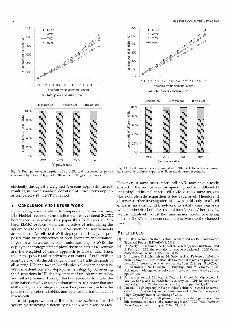
Figs. 8, 9, and 10 present the power consumption of all


0

40

80

120

160

200

0.1 0.2 0.3 0.4 0.5 0.6 0.7 0.8 0.9 1

downlink traffic demand (Mbps)

tota

lpow

er

of

all

eN

Bs

(W)

MCD

ATD

TKD

ours

(a) Total power consumption

0%

20%

40%

60%

80%

100%

MCD ATD TKD ours

pow

er

ratio

of

diffe

rent

eN

Bs

macro-cell micro-cell pico-cell

(b) power ratio

Fig. 7: Total power consumption of all eNBs and the ratios of powerconsumed by different types of eNBs in the small-group scenario.

eNBs and the ratios of power spent by different types of eNBsin the large-group, multi-group, and downtown scenarios,respectively. These results are similar to Fig. 7, where oureNB deployment strategy always allows eNBs to emit lesspower to satisfy the growing demand of UEs. Besides, theratio of power consumed by macro-cell eNBs in our eNBdeployment strategy is around 77.05%, 80.03%, and 73.53%in the large-group, multi-group, and downtown scenarios,respectively, which is significantly lower than that in the otherthree methods. Interestingly, in the downtown scenario, thepico-cell eNBs contribute more power consumption by theTKD method and our eNB deployment strategy, as shownin Fig. 10(b). Because UEs are scattered over streets in thisscenario, both methods prefer using more pico-cells to servesparse UEs, thereby increasing the corresponding power ratio.

6.3 Load Balance

Finally, we observe the standard deviation of the amount ofpower consumption of all macro-cell eNBs, which can be usedto estimate their load-balancing degree. In particular, a smallerstandard deviation indicates that most of macro-cell eNBscan emit the similar amount of transmission power, so theirtraffic loads are more balanced. By varying the downlink trafficdemands from UEs, Fig. 11 shows the experimental results.Obviously, because the MCD method considers homogeneousmacro-cell eNBs, it always results in the largest standarddeviation in different scenarios. On the other hand, the ATDmethod divides UEs into groups where the diameter of each

0

50

100

150

200

250

0.1 0.2 0.3 0.4 0.5 0.6 0.7 0.8 0.9 1


tota

lpow

er

of

all

eN

Bs

(W)

MCD

ATD

TKD

ours


0%

20%

40%

60%

80%

100%

MCD ATD TKD ours

pow

er

ratio

of

diffe

rent

eN

Bs


(b) power ratio

Fig. 8: Total power consumption of all eNBs and the ratios of powerconsumed by different types of eNBs in the large-group scenario.

group is no larger than Rmacro or Rmicro. In this case, somemacro-cells may cover only few UEs so as to increase the stan-dard deviation of power consumption. Both the TKD methodand our eNB deployment strategy employ the concept of K-means to group UEs based on their geographic relationships.Therefore, they seek to deploy macro-cell eNBs to cover similarnumber of UEs and thereby reduce the standard deviation ofpower consumption.

From Fig. 11, we can observe that the standard deviation ofpower consumption increases as the downlink traffic demandgrows. Such phenomena become more significant in the small-group and multi-group scenarios, as shown in Fig. 11(a) and(c). The reason is that UEs congregate in certain parts ofthe service area in these two scenarios. In particular, mostof UEs appear in the core of the service area in the small-group scenario (referring to Fig. 5(a)), while the multi-groupscenario obviously contains five groups of UEs (referring toFig. 5(c)). Due to such uneven distributions of UEs, the macro-cells deployed in the subregions where UEs congregate willcover a large number of UEs, while others may serve only asmall number of UEs. Thus, the standard deviation of powerconsumption substantially increases, especially when the traf-fic demands grow. In contrast with the above two scenarios,UEs are distributed over the service area more uniformly inboth the large-group and downtown scenarios (referring toFig. 5(b) and (d)). Therefore, the standard deviation of powerconsumption can be reduced in Fig. 11(b) and (d). In thesetwo cases, our eNB deployment strategy can group UEs more


0

200

400

600

800

1000

1200

0.1 0.2 0.3 0.4 0.5 0.6 0.7 0.8 0.9 1


tota

lpow

er

of

all

eN

Bs

(W)

MCD

ATD

TKD

ours


0%

20%

40%

60%

80%

100%

MCD ATD TKD ours

pow

er

ratio

of

diffe

rent

eN

Bs


(b) power ratio

Fig. 9: Total power consumption of all eNBs and the ratios of powerconsumed by different types of eNBs in the multi-group scenario.

efficiently through the weighted K-means approach, therebyresulting in lower standard deviation of power consumptionas compared with the TKD method.

7 CONCLUSION AND FUTURE WORK

By allowing various eNBs to cooperate in a service area,LTE HetNets become more flexible than conventional 2G/3Ghomogeneous networks. This paper thus formulates an NP-hard EDMC problem with the objective of minimizing thesystem cost to deploy an LTE HetNet such that user demandsare satisfied. An efficient eNB deployment strategy is pro-posed from the perspectives of both geometry and resource.In particular, based on the communication range of eNBs, thedeployment strategy first employs the modified AHC schemeand the weighted K-means approach to cluster UEs. Then,under the power and bandwidth constraints of each eNB, itadaptively adjusts the cell range to meet the traffic demands ofall serving UEs and tactically adds pico-cells when necessary.We also extend our eNB deployment strategy by consideringthe fluctuations in UE density, impact of uplink transmission,and cell interference. Through the four scenarios to model thedistribution of UEs, extensive simulation results show that oureNB deployment strategy can save the system cost, reduce thepower consumption of eNBs, and balance the traffic loads ofmacro-cells.

In this paper, we aim at the initial construction of an LTEsystem by deploying different types of eNBs in a service area.

0

50

100

150

200

250

300

0.1 0.2 0.3 0.4 0.5 0.6 0.7 0.8 0.9 1


tota

lpow

er

of

all

eN

Bs

(W)

MCD

ATD

TKD

ours


0%

20%

40%

60%

80%

100%

MCD ATD TKD ours

pow

er

ratio

of

diffe

rent

eN

Bs


(b) power ratio

Fig. 10: Total power consumption of all eNBs and the ratios of powerconsumed by different types of eNBs in the downtown scenario.

However, in some cases, macro-cell eNBs may have alreadyexisted in the service area for operating and it is difficult to‘redeploy’ additional macro-cell eNBs due to some reasons(for example, site acquisition is too expensive). Therefore, itdeserves further investigation of how to add only small-celleNBs in an existing LTE network to satisfy user demandswhile minimizing both the cost and interference. Alternatively,we can adaptively adjust the transmission power of existingmacro-cell eNBs to accommodate the network to the changeduser demands.

REFERENCES

[1] ITU Radiocommunication Sector, “Background on IMT-Advanced,”Technical Report, IMT-ADV/1, 2008.

[2] D. Astely, E. Dahlman, A. Furuskar, Y. Jading, M. Lindstrom, andS. Parkvall, “LTE: the evolution of mobile broadband,” IEEE Comm.Magazine, vol. 47, no. 4, pp. 44–51, 2009.

[3] S. Barbera, P.H. Michaelsen, M. Saily, and K. Pedersen, “Mobilityperformance of LTE co-channel deployment of macro and pico cells,”Proc. IEEE Wireless Comm. and Networking Conf., 2012, pp. 2863–2868.

[4] A. Khandekar, N. Bhushan, J. Tingfang, and V. Vanghi, “LTE-Advanced: heterogeneous networks,” European Wireless Conf., 2010,pp. 978–982.

[5] A. Damnjanovic, J. Montojo, Y. Wei, T. Ji, T. Luo, M. Vajapeyam, T.Yoo, O. Song, and D. Malladi, “A survey on 3GPP heterogeneousnetworks,” IEEE Wireless Comm., vol. 18, no. 3, pp. 10–21, 2011.

[6] Fujitsu, “High-capacity indoor wireless solutions: picocell or femto-cell?” http://www.fujitsu.com/downloads/TEL/fnc/whitepapers/High-Capacity-Indoor-Wireless.pdf, 2014.

[7] C. Lee and H. Kang, “Cell planning with capacity expansion in mo-bile communications: a tabu search approach,” IEEE Trans. VehicularTechnology, vol. 49, no. 5, pp. 1678–1691, 2000.


0

20

40

60

80

100

120

0.1 0.2 0.3 0.4 0.5 0.6 0.7 0.8 0.9 1


sta

ndard

devia

tion

of

pow

er

(mW

) MCD

ATD

TKD

ours


0

20

40

60

80

100

120

0.1 0.2 0.3 0.4 0.5 0.6 0.7 0.8 0.9 1


sta

ndard

devia

tion

of

pow

er

(mW

)

MCD

ATD

TKD

ours


0

20

40

60

80

100

120

0.1 0.2 0.3 0.4 0.5 0.6 0.7 0.8 0.9 1


sta

ndard

devia

tion

of

pow

er

(mW

)

MCD

ATD

TKD

ours


0

20

40

60

80

100

120

0.1 0.2 0.3 0.4 0.5 0.6 0.7 0.8 0.9 1


sta

ndard

devia

tion

of

pow

er

(mW

)

MCD

ATD

TKD

ours


Fig. 11: Comparison on the standard deviation of the amount of power consumed by macro-cell eNBs in different deployment methods.

[8] S. Hurley, “Planning effective cellular mobile radio networks,” IEEETrans. Vehicular Technology, vol. 51, no. 2, pp. 243–253, 2002.

[9] N. Weicker, G. Szabo, K. Weicker, and P. Widmayer, “Evolutionarymultiobjective optimization for base station transmitter placementwith frequency assignment,” IEEE Trans. Evolutionary Computation,vol. 7, no. 2, pp. 189–203, 2003.

[10] J. Kalvenes, J. Kennington, and E. Olinick, “Hierarchical cellularnetwork design with channel allocation,” European J. OperationalResearch, vol. 160, no. 1, pp. 3–18, 2005.

[11] E. Amaldi, A. Capone, and F. Malucelli, “Planning UMTS base stationlocation: optimization models with power control and algorithms ,”IEEE Trans. Wireless Comm., vol. 2, no. 5, pp. 939–952, 2003.

[12] J. Yang, M. Aydin, J. Zhang, and C. Maple, “UMTS base sationlocation planning: a mathematical model and heusirtic optimisationalgorithms,” IET Comm., vol. 1, no. 5, pp. 1007–1014, 2007.

[13] H.Y. Zhang, Y.G. Xi, and H.Y. Gu, “A rolling window optimizationmethod for large-scale WCDMA base stations planning problem,”European J. Operational Research, vol. 183, no. 1, pp. 370–383, 2007.

[14] E. Amaldi and A. Capone, “Radio planning and coverage optimiza-tion of 3G cellular networks,” Wireless Networks, vol. 14, no. 4, pp.435–447, 2008.

[15] C.K. Ting, C.N. Lee, H.C. Chang, and J.S. Wu, “Wireless hetero-geneous transmitter placement using multiobjective variable-lengthgenetic algorithm,” IEEE Trans. Systems, Man, and Cybernetics, Part B:Cybernetics, vol. 39, no. 4, pp. 945–958, 2009.

[16] S. Wang, W. Zhao, and C. Wang, “Budgeted cell planning for cellularnetworks with small cells,” IEEE Trans. Vehicular Technology, 2015.

[17] A. Simonsson, B. Hagerman, J. Chistoffersson, L. Klockar, C. Kout-simanis, and P. Cosimini, “LTE downlink inter-cell interference as-sessment in an existing GSM metropolitan deployment,” Proc. IEEEVehicular Technology Conf., 2010, pp. 1–5.

[18] Y. Wu, D. Zhang, H. Jiang, and Y. Wu, “A novel spectrum arrange-ment scheme for femto cell deployment in LTE macro cells,” Proc.IEEE Int’l Symp. Personal, Indoor and Mobile Radio Comm., 2009, pp.6–11.

[19] P. Lin, J. Zhang, Y. Chen, and Q. Zhang, “Macro-femto heterogeneous

network deployment and management: from business models totechnical solutions,” IEEE Wireless Comm., vol. 18, no. 3, pp. 64–70,2011.

[20] S. Kaneko, T. Matsunaka, and Y. Kishi, “A cell-planning model forHetNet with CRE and TDM-ICIC in LTE-Advanced,” Proc. IEEEVehicular Technology Conf., 2012, pp. 1–5.

[21] X. Gelabert, G. Zhou, and P. Legg, “Mobility performance and suit-ability of macro cell power-off in LTE dense small cell HetNets,” Proc.IEEE Int’l Workshop on Computer Aided Modeling and Design of Comm.Links and Networks, 2013, pp. 99–103.

[22] W. Zhao and S. Wang, “Cell planning for heterogeneous cellularnetworks,” Prco. IEEE Wireless Comm. and Networking Conf., 2013, pp.1032–1037.

[23] W. Zhao, S. Wang, C. Wang, and X. Wu, “Cell planning for heteroge-neous networks: an approximation algorithm,” proc. IEEE INFOCOM,2014, pp. 1087–1095.

[24] E. Dahlman, S. Parkvall, and J. Skold, 4G: LTE/LTE-Advanced for MobileBroadband, Elsevier, 2013.

[25] M. Dottling, W. Mohr, and A. Osseiran, Radio Technologies and Conceptsfor IMT-Advanced, Wiley, 2009.

[26] European Telecommunications Standards Institute, “LTE; EvolvedUniversal Terrestrial Radio Access (E-UTRA); Radio Frequency (RF)requirements for LTE Pico Node B,” Technical Report, ETSI TR 136931 V9.0.0, 2011.

[27] E.L. Crow and K. Shimizu, Lognormal Distributions: Theory and Appli-cation, CRC Press, 1987.

[28] P. Dent, G.E. Bottomley, and T. Croft, “Jakes fading model revisited,”Electronics Letters, vol. 29, no. 13, pp. 1162–1163, 1993.

[29] E.P. Caspers, S.H. Yeung, T.K. Sarkar, A. Garcia-Lamperez, M.S.Palma, M.A. Lagunas, and A. Perez-Neira, “Analysis of informationand power transfer in wireless communications,” IEEE Antennas andPropagation Magazine, vol. 55, no. 3, pp. 82–95, 2013.

[30] D. Defays, “An efficient algorithm for a complete link method,”Computer J., vol. 20, no. 4, pp. 364–366, 1976.

[31] J. Han and M. Kamber, Data Mining: Concepts and Techniques, Aca-demic Press, 2001.


[32] C.E. Shannon, “A mathematical theory of communication,” Bell Sys-tem Technical J., vol. 27, pp. 379–423, 1948.

[33] A.J. Goldsmith and S. G. Chua, “Variable-rate variable-power MQAMfor fading channels,” IEEE Trans. Comm., vol. 45, no. 10, pp. 1218–1230, 1997.

[34] Y.C. Wang, Y.F. Chen, and Y.C. Tseng, “Using rotatable and direc-tional (R&D) sensors to achieve temporal coverage of objects and itssurveillance application,” IEEE Trans. Mobile Computing, vol. 11, no.8, pp. 1358–1371, 2012.

[35] L. Chen, Y. Huang, F. Xie, Y. Gao, L. Chu, H. He, Y. Li, F. Liang,and Y. Yuan, “Mobile relay in LTE-advanced systems,” IEEE Comm.Magazine, vol. 51, no. 11, pp. 144–151, 2013.

[36] J. Kokkoniemi, J. Ylitalo, P. Luoto, S. Scott, J. Leinonen, and M. Latva-aho, “Performance evaluation of vehicular LTE mobile relay nodes,”Proc. IEEE Int’l Symp. Personal Indoor and Mobile Radio Comm., 2013,pp. 1972–1976.

[37] W. Debus, “RF path loss & transmission distance calculations,” Ax-onn Technical Memorandum, 2006.

[38] A.S. Hamza, S.S. Khalifa, H.S. Hamza, and K. Elsayed, “A surveyon inter-cell interference coordination techniques in OFDMA-basedcellular networks,” IEEE Comm. Surveys & Tutorials, vol. 15, no. 4, pp.1642–1670, 2013.

ELSEVIER COMPUTER NETWORKS 1 Efﬁcient eNB …wangyc/publications/journals/j024...Efﬁcient eNB...

Documents

Transcript of ELSEVIER COMPUTER NETWORKS 1 Efﬁcient eNB …wangyc/publications/journals/j024...Efﬁcient eNB...