Elliott Parker. Mark Pingle The distributional effects of ...

DOI 10.1007/s00181-005-0046-1

ORIGINAL PAPER

Elliott Parker . Mark Pingle

The distributional effects of selectionand capital accumulation on firmproductivity under imperfect capital markets

Received: 12 July 2004 / Accepted: 5 July 2005© Springer-Verlag 2005

Abstract In this evolutionary model, random shocks create differences in the rateof return on capital, while individual saving and investment behavior can reducethese differences over time. Firms with either low total factor productivity (TFP) ora low average return on capital are selected for exit, and new firms enter to taketheir place. As would be expected, a higher turnover rate improves TFP andreduces its variation. While we show that a higher turnover rate would result in amore positively skewed TFP distribution if exit selection is based directly uponTFP, we find that when we select firms for exit based on their average product ofcapital, the marginal impact of a higher turnover rate is to more negatively skew theTFP distribution. Overall, our simulations highlight the importance of consideringthe role selection may play in shaping the distribution of productivity wheneconometricians seek estimates of firm inefficiency.

Keywords Firm evolution . Selection . Total factor productivity . Productivitydistribution

JEL Classification D2 . D9 . O3

1 Introduction

There is growing evidence that productivity improvements result more from aselection process, which reallocates resources from less productive to moreproductive firms, than from the improvement of the typical firm. A growingnumber of empirical studies (e.g., Bartelsman and Dhrymes 1998; Dwyer 1998;Foster et al. 1998; Levinsohn and Petrin 1999; and Rigby and Essletzbichler 2000)are finding evidence that aggregate productivity improvements are largely

E. Parker (*) . M. PingleDepartment of Economics /030, University of Nevada, Reno, NV 89557-0207, USAE-mail: [email protected]

Empirical Economics

explained by the expansion of more productive firms, the contraction of lessproductive firms, and the entry of new firms. Individually, firms often appear to betrapped in their past choices so that their productivity remains relatively stagnant.Montgomery and Wascher (1988) find evidence that the rate of business failuressignificantly affects the rate of aggregate productivity growth. As a result of theseand other studies, there is a growing recognition of the importance of Schum-peterian creative destruction in any market economy.

If selection processes are important, then the gradual elimination of lessproductive firms could observably affect the skew of the distribution of firmproductivity, not just the mean or variance. That is, it is conceivable that the skewof the productivity distribution could be used to test for the presence of competitionin the form of a selection process. To our knowledge, no previous study hasrecognized this. For example, we might be more likely to observe a more positiveskew in a sample of U.S. restaurants where the market is competitive and selectionregularly eliminates the poorest performers than in a sample of Japanese banks orChinese state-owned enterprises subject to government no-failure policies. Thesuccess of an economic liberalization effort could conceivably be measured by theobserved changes in the skew of the productivity distribution.

However, the issue is not as simple as it may first appear. Productivity must bedefined and how a firm is selected for exit is open to question. When we speak ofthe productivity distribution, we are specifically referring to the distribution of“total factor productivity,” or TFP. TFP can be considered a measure of thetechnology level of the firm or a measure of the extent to which the firm uses thebest available business practices. Empirical studies that seek to measure technicalinefficiency or use the concept to estimate the location of a stochastic frontiertypically rely upon certain assumptions about the TFP distribution.1

An alternative measure of productivity is the average product of capital. Thisproductivity measure is more directly associated with the health of the firm in theeyes of the firm’s owner, who is forgoing consumption to supply the firm withcapital. Below, we illustrate that a selection criterion that forces firms at the lowertail of the TFP distribution to exit will tend to create a positive skew in the TFPdistribution. This is not particularly surprising, but provides a basis for comparison.Our primary interest is examining how a selection process that forces out the firmswith the lowest average product of capital (which we use as a proxy for firmprofitability) will impact the skew of the TFP distribution.

When selection is based upon the productivity of capital, it is not clear how thedistribution of total factor productivity will change over time. Suppose two firmswith the same capital stock level innovate differently so that the marginal productof capital is higher for the firm that discovers the better technology or businesspractice. Under normal market conditions, a larger marginal product of capitalprovides a higher rate of return on capital, which provides a stronger incentive toaccumulate capital. However, in the standard model of the firm, the marginalproduct of capital decreases as capital increases. Thus, the firm that innovates moreeffectively will find that diminishing returns reduces its competitive advantage. Afirm with a better technology could be selected for exit over a firm with a poorertechnology if capital accumulation and diminishing returns sufficiently reduces the

1Kumbhakar and Orea (2004) and Giannakas et al. (2003) are recent examples of this type ofresearch in this journal.

E. Parker and M. Pingle

profitability of the firm. Will selection weed out the worst technologies andbusiness practices, creating a positive skew in the TFP distribution, or can lesseffective technologies and business practices persist in smaller firms where smallercapital stocks help buttress a higher marginal productivity of capital? Because theanswer to this question is not theoretically clear, we use simulation to explore theissue.

In our model, investment must be financed out of current income, so we areimplicitly ignoring the important role that financial markets can play in reallocatingone firm’s savings to another firm’s investment. This abstraction allows us tomaintain tractability but it is also not exceptionally troublesome. A perfect capitalmarket would provide immediate convergence of capital productivity and rates ofreturn on capital as less innovative firms transferred of their capital to the moreinnovative firms. So, who would be selected for exit? Our model is useful becausethe absence of capital market allows the productivity of capital to vary across firms.This allows us to select firms on the basis of capital productivity and makes itpossible to produce a model where the productivity of capital for different firms canconverge over time.

In our model we also do not allow immediate TFP catch up through imitation orfree discrete jumps to the best available technology, for this would obviouslygenerate a negative skew in the TFP distribution. Instead, we assume that firms arelocked into their past decisions and investments. New firms can imitate, however,and we assume that they enter with a productivity level that is randomly distributedabout the mean productivity level of the existing firms. Existing firms experienceproductivity shocks each period under the assumption that they try an innovationthat may or may not be fruitful. Thus, our model directly recognizes constraints onlearning. While these constraints keep the productivity distribution from readilyachieving a negative skew, the randomness we assume does not bias thedistribution toward a positive skew.

Our primary finding is that if the selection method is based upon averageproductivity of capital, then a higher rate of selection (entry and exit) leads to afaster-rising mean level of total factor productivity, a slower-rising variance, and anegative marginal effect on skew. The simulation illustrates that large firms withhigher total factor productivity may nonetheless be selected for exit because capitalaccumulation in the face of diminishing returns leads to a relatively lowproductivity of capital. Firms learn in our model, in the sense that they re-optimizetheir savings and investment choices each period. However, firms are locked intopast investment choices, and negative productivity shocks can suddenly makethese choices not only less than optimal, but also non-competitive enough that thefirm is selected for exit.

The paper is organized as follows. In Section 2, we present the issues relating tothe distribution of firm productivity in some detail, and review some previouswork. In Section 3, we present our model of the firm sector. In Section 4, wesimulate the model once, examining how the mean, variance, and skew of totalfactor productivity respond to changes in the selection rate. In Section 5, wesimulate the model 6000 times, varying not only the selection rate but also otherparameters so as to examine the robustness of impact of changes in the selectionrate. Some concluding remarks are presented in Section 6.

The distributional effects of selection and capital accumulation

2 Optimization, evolution, and firm productivity

Choice plays a different role in traditional neoclassical economic theory than itdoes in the growing literature on economic evolution. In the neoclassical frame-work, rational, self-interested, and well-informed individuals with similarpreferences and incentives make similar choices, and differences are usuallytreated as white noise. The assumption that any given activity yields diminishingreturns helps keep differences between the best and worst performers to aminimum, and a convergence of performance is typically expected. In contrast, thetypical model in evolutionary biology presents individuals as being constrained byprocesses beyond their individual control, so individual choices are not veryimportant. The possibility of increasing returns makes increasing divergence apossibility, while path-dependence may also amplify initially minor differences.

Rational decision-making may arise in an evolutionary model. However, to doso, it must evolve over time. Textbook biology presents four conditions-variation,selection (competition), transmission (heredity), and iteration (time)-as beingnecessary for evolution. Pinker (1997) has argued that, if behavior has a geneticcomponent, evolution can result in the selection of unintentional optimizingbehavior, given enough time. Likewise, Alchian (1950) demonstrated that rationalprofit-maximizing behaviors could result from an evolutionary selection processeven if firm managers were not particularly rational. Thus, there is reason toassume that prior evolutionary processes have created a population of forwardlooking, rational decision-makers, but that continuing evolutionary processesprevent decision-makers from actually implementing their plans very far into thefuture.

We use the optimizing framework of Ramsey (1928), Cass (1965), andKoopmans (1965) to make our agents forward-looking, while introducing anevolutionary process that meets these four conditions and forces the forward-looking agents to repeatedly update their plans.2 As the economy unfolds iterationby iteration in our experiment, we can observe the impact of the optimizingbehavior combined with the evolutionary process on the distribution of firm totalfactor productivity (TFP).

Changes in TFP can lead to differences in firm profitability. Factors affectingTFP could include production technologies, managerial methods, and intangibleinput qualities. Let ait denote the TFP of firm i during period t. A typical model ofproduction is

yit ¼ ait f kit; litð Þ (1)

where yit, kit, and lit are the output, capital input, and labor input levels for firm i attime t.

Holding the effects of functional form constant, Fig. 1a presents a TFPdistribution which would result if the errors firms make in their technology andmanagement choices are random, but normally distributed around some centraltendency.

2 In doing so, we are following Jovanovic (1982), who cites evidence that small firms grow fasterthan large firms but are also more likely to fail, and creates a model of “‘noisy’ selection” toexplain why.


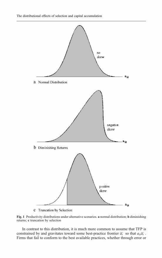
In contrast to this distribution, it is much more common to assume that TFP isconstrained by and gravitates toward some best-practice frontier at so that aitat .Firms that fail to conform to the best available practices, whether through error or

Fig. 1 Productivity distributions under alternative scenarios. a normal distribution; b diminishingreturns; c truncation by selection


poorly-designed incentives, will produce inside the observable frontier rather thanon it. The stochastic frontier econometric approach, developed by Aigner et al.(1977), assumes productivity differentials can be decomposed into two parts, sothat

ait ¼ at þ uit þ �it: (2)

Here, uit is a normally distributed white-noise measurement error and νit≤0 isthe firm’s inefficiency, with a half-normal, exponential/gamma, or truncatednormal distribution. These distributional assumptions imply observed TFP shouldpossess a significant negative skew as shown in Fig. 1b as firms gravitate towardthe best available practices.

However, not all firm-level data sets appear to have the expected negative skew.Green and Mayes (1991) attempted to estimate stochastic frontier productionfunctions for firms in hundreds of different industries across several differentcountries, and found significant proportions-over half in the United Kingdom andthe United States, and over a third in Australia-that either had a positive skew or anexcessively small variance in the white-noise component relative to the skewedcomponent. Carree (2002) cites other, similar evidence.

In part because actual data sets often do not have the expected negative skew,the data envelopment approach, developed by Charnes et al. (1978), has becomeincreasingly popular. It uses the equation

ait ¼ at exp eitð Þ (3)

where êit≤0 is the resulting one-sided firm-specific error term, in order to find theproduction surface that envelops the observations for the different firms.3 Althoughit has the disadvantage of being sensitive to the mismeasurement of firms on thefrontier, this non-stochastic approach makes no assumptions regarding the skew offirm TFP.

Why are econometricians finding that different frontier approaches are useful indifferent cases? We explore the notion that the distribution of TFP may change asthe economy evolves. Entrepreneurs are constantly innovating, which leads to newproducts, new methods of production, and new management methods. Techno-logical progress changes the relative profitability of firms. In this Schumpeterianworld of creative destruction, the actions of successful innovators lead to theelimination of those less successful through a competitive selection mechanismlike bankruptcy.4

If firms make innovations with results that are a priori unknown, then we shouldexpect the results to be essentially random, and the variance of TFP should growover time. If a selection process then works to remove the firms with the lowestTFP from the population, and new entrants are able to enter with higher TFP thanthose who have exited, then we might expect that the distribution of TFP wouldbecome more positively skewed over time as in Fig. 1c, in contrast to the stochasticfrontier approach’s assumption of negative skew.

3As of June, 2001, when this research began, Econlit listed 217 citations for the stochastic frontierapproach since 1977, and 365 citations for the data envelopment approach since 1985. In the pastfew years, citations for the former approach are around half those for the latter approach,suggesting that the former method is gradually being replaced by the latter.4 See, for example, Ericson and Pakes (1995) for a description and model of this process.


Because the shape of the TFP distribution is an important issue for econometricwork, it is useful to know how selection affects the distribution. Even if theabsolute distribution depends a variety of factors, knowing the marginal impact ofselection on mean, variance, and skew to may facilitate the construction of a test forthe presence of selection. The simulations we perform below inform us about howselection affects the distribution of TFP.

3 The model

Assume a sector of the economy consists of N single-person firms, who mustfinance their investment out of personal savings. The consumption level c for firm iat time t is chosen by each consumer/firm to maximize inter-temporal utility, withindividual-specific discount rate ρ and elasticity of substitution θ. The firm’s capitalstock k grows by its income less consumption and depreciation, where thedepreciation rate is δ. The firm’s income is a constant-returns-to-scale Cobb–Douglas function of the firm’s TFP level a and its capital stock (since labor for asingle person firm is unity). The output elasticity of capital is assumed to be equalacross firms, but productivity is assumed to be firm-specific because of continuousinnovations in product differences, labor quality, or managerial methods.Following Barro and Sala-I-Martin (1995), the resulting growth model is asfollows:

max

Z1

0

ui citð Þe��i t@t; where ui citð Þ ¼ c1��iit � 1

1� �i(4)

subject to:

ki�@k@t ¼ g cit; kitð Þ ¼ yit � cit � �kit

yit ¼ ait f kit; litð Þf kit; litð Þ ¼ k �

it11�� ¼ aitk�it

cit � yit

The Hamiltonian for this problem is:

H Cit; kit; �itð Þ ¼ c1��it � 1

1� �ie��i t þ �it aitk

�it � cit � �kit

� �(5)

with the following first-order conditions:

@H@cit

¼ c��iit e��i t � �it ¼ 0

@H@kit

¼ �it �ait k��1it � �

� � ¼ ��it

limt!1�itkit ¼ 0

ð4:aÞð4:bÞð4:cÞð4:dÞ

5:að Þ5:bð Þ5:cð Þ


The differential equations obtained from the first order conditions are:

að Þ ci� ¼ �ai k ��1

i � �� i� �

ci�i

bð Þ ki�¼ ai k �

i � ci � �ki� � (6)

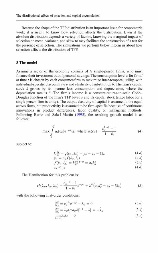
In Fig. 2, we show the traditional phase diagram for these two equations. Thestable arm for the system shown in the figure is the optimal path of consumptionand the capital stock.

3.1 Optimization

Given the current capital stock level ki0, the firm owner’s immediate problem is thatof finding the optimal current consumption level ci0, which simultaneouslydetermines the optimal current saving and investment levels. Finding this level inthe phase diagram is a simple matter, as shown in Fig. 2. However, finding aparticular numerical value for current consumption, given values for all of themodel’s parameters, is more involved. To do so, we use the time-eliminationmethod described by Barro and Sala-I-Martin (1995). It first requires finding thesteady-state levels:

að Þ ki�¼ � ai

�iþ�

� �11��

bð Þ ci� ¼ � ai k �

i � �ki� � (7)

Then the slope of the stable growth path must be calculated, which is:

@ci@ki

¼ c�i

ki� ¼

� ai k ��1i � �� i

� �ci

ai k �i � ci � �kið Þ�i (8)

Fig. 2 Phase diagram for Ramsey growth model


This slope must then be evaluated at the steady state. Because the denominatorki and numerator ċi are both equal to zero in the steady state, we must evaluate thederivative (Eq. 8) at the steady state using L’Hôpital’s rule. After some algebra, wefind that at the steady state the derivative (Eq. 8) becomes:

@ci@ki

¼@c�i

@ki

� �@k�i

@ki

� � ¼ 12 �i þffiffiffiffiffiffiffiffiffiffiffiffiffiffiffiffiffiffiffiffiffiffiffiffiffiffiffiffiffiffiffiffiffiffiffiffiffiffiffiffiffiffiffiffiffiffiffiffiffiffiffiffi�2i � 4ai � �� 1ð Þk��2

i ci=�i

q� �(9)

The final step is to use Euler’s method to follow the stable arm shown in Fig. 2from the steady state value to an approximation of the location of the point (ki0, ci0).When Z steps (where Z corresponds not to any time period, but instead to thenumber of steps necessary to accurately trace the nonlinear path) are taken en routefrom the steady state to the initial state, the change in capital that occurs upon eachstep is

�ki ¼ kit � ki0Z

� (10.a)

The path for capital, going backwards in time from the steady state, can then besimulated as

ki t�1ð Þ ¼ kit ��ki; (10.b)

where the initial value (working backwards) for kit for is ki . We can then simulatethe path for consumption using

ci t�1ð Þ ¼ cti � @cit@kit

�ki; (10.c)

where the initial value for cit for is ci , the initial value of @cit=@kit is given by Eq.(9), and all but the initial value of @cit=@kit is given by Eq. (8) Upon completingstep Z, we have worked our way backwards down the optimal consumption growthpath to an estimated location of the point (ki0,ci0). The value obtained for ci0 is theestimated optimal current consumption level for the firm that is consistent with thefirm’s specific capital stock ki0, TFP level ai0, individual parameters ρi and θi, andshared parameters α and δ.

We assume here that firms must finance their own investments, and thissimplifies the optimization process considerably because a market process forcapital reallocation is somewhat difficult to simulate with heterogeneous firms.5

Such grossly imperfect capital markets are an extreme assumption, but our purposein this model is to create a controlled experiment in which we can isolate the effectsof selection on distribution. In a perfectly efficient capital market, we would expectthat the variance (and skew) of profit rates would converge to zero in the presenceof diminishing returns, since any shock to productivity would immediately beoffset by a movement of capital in or out of the firm. We thus choose to consider theother extreme, in which a firm is locked into its own past investments.

5 Cargill and Parker (2002) used a simulation of a Walrasian tattonment process, but it iscomputationally demanding.


3.2 Productivity shocks

While each firm faces the same output elasticity α of capital and capitaldepreciation rate δ, our firm sector is perturbed by varying levels of entrepreneur-ship, and each firm is constantly experimenting with new innovations. Since theoutcomes of these innovations are not known in advance, we follow Jovanovic(1982) by assuming the firm’s TFP level is subject to additive random shocks, sothat it becomes a random walk: 6

ait ¼ ai;t�1 þ "it; where "it � N �; �2� �� (11)

Because variations in the outcomes of innovation efforts affect TFP, whilevariations in individual preferences affect consumption choices, some individual/firms will be more successful than others even though all are optimizing. In amarket in which firms compete for resources, poor performers may exit, eitherbecause they choose to do so in order to find more lucrative alternatives or becausethey are forced to do so because of a mechanism such as bankruptcy andliquidation. We assume firms can be sorted according to observable successcriteria, and for simplicity we assume the fraction χ of firms exiting the market inany period is exogenously determined.

In this model, the firm is choosing the optimal rate of savings and investment ineach period, in order to maximize intertemporal utility, but these productivityshocks are unexpected. Thus, a negative shock can mean that a firm’s pastinvestments suddenly become suboptimal, and a larger firm (which presumablybecame larger because it was relatively productive in the past) may find its sizeworking against it due to diminishing returns. If the shock is large, then the firmmay not survive, but if it does survive then it would reduce its rate of futureinvestment in response. To some extent, this continual re-optimization is a little likelearning, though we do not model that explicitly.

3.3 Selection

What success criterion should we use? One reasonable criterion would be toassume that a firm would will voluntarily exit a market if the expected long-run rateof return, calculated using an appropriate risk-adjusted discount rate, is less thanthat available elsewhere.7 Cargill and Parker (2002) used such a criterion, shuttingdown firms when the profit level falls below the wage level less a fixed shutdowncost.

6 Parker (1995) and Cargill and Parker (2002) assumed that this shock was exponentially normal,of the form ait ¼ ai;t�1 e"it . While this has the benefit of ensuring that TFP is always positive, itbiases the results towards a positive skew. However, we tested the simulation in Section 4 by re-running it with the exponential shock; in re-estimating the response function, we found themarginal effects not significantly affected.7 Of course, bankruptcy as a legal process is rarely so optimal. Managers may be willing tocontinue operating a loss-making firm if they can hide information on the firm’s poor long-runpotential from the owners. Creditors with first priority of repayment may force a potentiallyproductive firm to liquidate to ensure that they do not have to accept a loss on their investment.


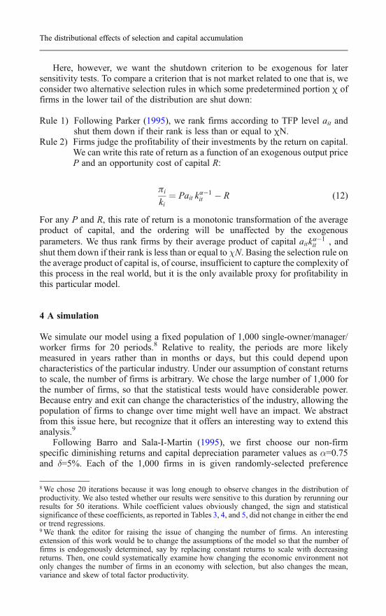
Here, however, we want the shutdown criterion to be exogenous for latersensitivity tests. To compare a criterion that is not market related to one that is, weconsider two alternative selection rules in which some predetermined portion χ offirms in the lower tail of the distribution are shut down:

Rule 1) Following Parker (1995), we rank firms according to TFP level ait andshut them down if their rank is less than or equal to χN.

Rule 2) Firms judge the profitability of their investments by the return on capital.We can write this rate of return as a function of an exogenous output priceP and an opportunity cost of capital R:

i

ki¼ Pait k

��1it � R (12)

For any P and R, this rate of return is a monotonic transformation of the averageproduct of capital, and the ordering will be unaffected by the exogenousparameters. We thus rank firms by their average product of capital aitk��1

it , andshut them down if their rank is less than or equal to χN. Basing the selection rule onthe average product of capital is, of course, insufficient to capture the complexity ofthis process in the real world, but it is the only available proxy for profitability inthis particular model.

4 A simulation

We simulate our model using a fixed population of 1,000 single-owner/manager/worker firms for 20 periods.8 Relative to reality, the periods are more likelymeasured in years rather than in months or days, but this could depend uponcharacteristics of the particular industry. Under our assumption of constant returnsto scale, the number of firms is arbitrary. We chose the large number of 1,000 forthe number of firms, so that the statistical tests would have considerable power.Because entry and exit can change the characteristics of the industry, allowing thepopulation of firms to change over time might well have an impact. We abstractfrom this issue here, but recognize that it offers an interesting way to extend thisanalysis.9

Following Barro and Sala-I-Martin (1995), we first choose our non-firmspecific diminishing returns and capital depreciation parameter values as α=0.75and δ=5%. Each of the 1,000 firms in is given randomly-selected preference

8We chose 20 iterations because it was long enough to observe changes in the distribution ofproductivity. We also tested whether our results were sensitive to this duration by rerunning ourresults for 50 iterations. While coefficient values obviously changed, the sign and statisticalsignificance of these coefficients, as reported in Tables 3, 4, and 5, did not change in either the endor trend regressions.9We thank the editor for raising the issue of changing the number of firms. An interestingextension of this work would be to change the assumptions of the model so that the number offirms is endogenously determined, say by replacing constant returns to scale with decreasingreturns. Then, one could systematically examine how changing the economic environment notonly changes the number of firms in an economy with selection, but also changes the mean,variance and skew of total factor productivity.


parameters θ and ρ, where θ is distributed uniformly between 0.5 and 3.5, and ρ isdistributed uniformly between 0.02 and 0.08.10 Each firm is endowed with theproductivity level ai0 =1 and an initial capital stock equal to 10% of the initialsteady state:

ki;0 ¼ 0:10� 0:75� 1:00

0:05þ 0:05

� � 11�:75

� 316:4; for all i: (13)

In each period, firm innovation first leads to productivity shocks as describedby Eq. (11). We set the normal distribution parameters as μ=0 and σ=0.04, so thereis firm variation but no inherent trend of productivity improvement. Firms produceoutput given existing productivity and capital stock (Eq. 4c). Firms then eachchoose their current optimal consumption level (Eqs. 4.a through 10.c), where thenumber of steps taken in iterating the Euler equation was chosen to be Z=25.11

Capital stock accumulates through savings (Eq. 4.a) subject to the incomeconstraint (Eq. 4.b), and both for simplicity’s sake and because we want currentdecisions to depend in part on past performance, we assume there is no capitalmarket and firms must rely on their own savings. Finally, firms are sorted on thebasis of the selection criterion (either ai or π/k), and the poorest χ=5% are forced toexit. New entrants begin with the initial capital stock given by Eq. (13) andrandomly-selected preference parameters, but their initial TFP level is equal to theoutput-weighted mean of the surviving firms. We iterate this procedure 20 times.

Figures 3, 4 and 5 show histograms for total factor productivity. 12 Figure 3shows the results of no selection, or entry and exit, at all. Figures 4 and 5 show theresults of implementing exit selection rules 1 and 2, along with replacement entry.A histogram is shown for the initial period t=1 and the final period t=20.

When there is no entry and no exit, as Fig. 3 shows, the distribution of TFP isnot skewed in either direction. When we select according to firm’s TFP, as Fig. 4shows, the distribution of TFP acquires a positive skew, as expected. When weselect using the average product of capital as our criterion, however, we obtainqualitatively different results. As we can see in Fig. 5, there appears to be nopositive skew. This can occur because a firm with a higher level of TFP maynonetheless be selected for exit when it has accumulated a significant amount ofcapital. The reduction in the average product of capital because of diminishingreturns may be more than enough to offset the increase in average product causedby the higher level of TFP.

For each of our three cases we report in Table 1, we give the ending meanvalues M(·) for firm total factor productivity ai, along with the coefficient ofvariation and a coefficient of skewness. For some randomly distributed variable x,

10 The changes in these preference parameters did not significantly influence the results.11We simulated the estimation of current consumption with different parameter sets for manyvalues of Z. We found that consumption estimates were wildly unstable for values of Z below 5,so the stable arm of the growth path is clearly not linear. However, for Z ≥10, we found that theconsumption estimates started to converge asymptotically. The estimates obtained for Z=25 werevery close to the estimates for T=10,000.12 Each case is a separate simulation, and small differences are to be expected due to differences inthe random shocks.


with mean μx and standard deviation σx, the coefficient of variation is V(x) = σx/μx,and the coefficient of skewness S(x) is

S xð Þ ¼ 1

N

XNi¼1

xi � �x

�x

� �3

: (14)

Examining firm productivity, we find that TFP does not improve over 20periods when there is no selection. Conversely, both selection rules result in

OO OO XXOO OOXXOO OOXXOOXXOO OOXXOOXXOO OOXXOOXXOO OOXXOOXXOOXX OO OOXXOOXXOOXX XX OOXXOOXXOOXXOOXX XX OOXXOOXXOOXXOOXX XX XX OOXXOOXXOOXXOOXXOOXX XX XXOOXXOOXXOOXXOOXXOOXX XXOOXXOOXXOOXXOOXXOOXXOOXX XXOOXXOOXXOOXXOOXXOOXXOOXXOO XXOOXXOOXXOOXXOOXXOOXXOOXXOO OOXXOOXXOOXXOOXXOOXXOOXXOOXXOO XXOOXXOOXXOOXXOOXXOOXXOOXXOOXXOOXX XXOOXXOOXXOOXXOOXXOOXXOOXXOOXXOOXXOO OOXXOOXXOOXXOOXXOOXXOOXXOOXXOOXXOOXXOOXX OOXXOOXXOOXXOOXXOOXXOOXXOOXXOOXXOOXXOOXX |XX OOXXOOXXOOXXOOXXOOXXOOXXOOXXOOXXOOXXOOXXOOXXOOXX |XXOOXXOOXXOOXXOOXXOOXXOOXXOOXXOOXXOOXXOOXXOOXXOOXXOOXXOOXXOO |---------|---------|---------|---------|---------|---------| 0.88 0.92 0.96 1.00 1.04 1.08 1.12

a Period 1: M(a) = 1.00, V(a) = 0.04, S(a) = -0.12

XX XX XX XX XX XX XXOO XXOOXXOO XXOOXXOO OOXXOOXXOO OO OOXXOOXXOO XXOOXXOOXXOOXXOOXX XXOOXXOOXXOOXXOOXX XXOOXXOOXXOOXXOOXX XX OOXXOOXXOOXXOOXXOOXXOOXX OOXXOOXXOOXXOOXXOOXXOOXX XXOOXXOOXXOOXXOOXXOOXXOOXX XXOOXXOOXXOOXXOOXXOOXXOOXXOO XXOOXXOOXXOOXXOOXXOOXXOOXXOO XXOOXXOOXXOOXXOOXXOOXXOOXXOO XXOOXXOOXXOOXXOOXXOOXXOOXXOOXXOO XXOOXXOOXXOOXXOOXXOOXXOOXXOOXXOOXXOO OOXXOOXXOOXXOOXXOOXXOOXXOOXXOOXXOOXXOO OOXXOOXXOOXXOOXXOOXXOOXXOOXXOOXXOOXXOOXXOO |XX XXOOXXOOXXOOXXOOXXOOXXOOXXOOXXOOXXOOXXOOXXOO XX |XXOOXXOOXXOOXXOOXXOOXXOOXXOOXXOOXXOOXXOOXXOOXXOOXXOOXXOOXXOO |---------|---------|---------|---------|---------|---------| 0.48 0.66 0.83 1.00 1.17 1.34 1.51

b Period 20: M(a) =1.00, V(a) = 0.17, S(a) = -0.00

Fig. 3 Total factor productivity without selection


significant improvements in total factor productivity. While the variation of TFPstill increases over the 20 periods, both selection methods lead to a reduction in thevariance relative to having no selection. Consistent with what we can observe inFigs. 4 and 5, the skew of the distribution is very positive under selection rule 1(using ait), while under selection rule 2 (using aitk

α−1) the skew is approximatelyzero, as it is when there is no selection.

OO OO OO OOXXOO OOXXOO OOXXOOXX OOXXOOXX XXOOXXOOXXOOXX XXOOXXOOXXOOXX XXOOXXOOXXOOXX XXOOXXOOXXOOXXOOXXOO XXOOXXOOXXOOXXOOXXOO XXOOXXOOXXOOXXOOXXOO OOXXOOXXOOXXOOXXOOXXOO OOXXOOXXOOXXOOXXOOXXOO OOXXOOXXOOXXOOXXOOXXOOXX XXOOXXOOXXOOXXOOXXOOXXOOXXOO XXOOXXOOXXOOXXOOXXOOXXOOXXOOXX XXOOXXOOXXOOXXOOXXOOXXOOXXOOXXOOXX XXOOXXOOXXOOXXOOXXOOXXOOXXOOXXOOXXOO OOXXOOXXOOXXOOXXOOXXOOXXOOXXOOXXOOXXOOXX XXOOXXOOXXOOXXOOXXOOXXOOXXOOXXOOXXOOXXOOXX XX OOXXOOXXOOXXOOXXOOXXOOXXOOXXOOXXOOXXOOXXOOXXOOXX

|XXOOXXOOXXOOXXOOXXOOXXOOXXOOXXOOXXOOXXOOXXOOXXOOXXOOXXOOXXOO |---------|---------|---------|---------|---------|---------| 0.88 0.92 0.96 1.00 1.04 1.08 1.12

a Period 1: M(a) =1.00, V(a) = 0.04, S(a) = 0.03

XX XX XX XXOOXX XX XXOOXX XX XXOOXX XXOOXXOOXX OOXXOOXXOOXX OOXXOOXXOOXX XXOOXXOOXXOOXX XXOOXXOOXXOOXX XXOOXXOOXXOOXXOO XXOOXXOOXXOOXXOOXX OOXXOOXXOOXXOOXXOOXX XXOOXXOOXXOOXXOOXXOOXX XXOOXXOOXXOOXXOOXXOOXX XXOOXXOOXXOOXXOOXXOOXXOOXX XXOOXXOOXXOOXXOOXXOOXXOOXX OOXXOOXXOOXXOOXXOOXXOOXXOOXXOO OOXXOOXXOOXXOOXXOOXXOOXXOOXXOO OOXXOOXXOOXXOOXXOOXXOOXXOOXXOOXXOO XXOOXXOOXXOOXXOOXXOOXXOOXXOOXXOOXXOO OOXXOOXXOOXXOOXXOOXXOOXXOOXXOOXXOOXXOOXX XX OO OOXXOOXXOOXXOOXXOOXXOOXXOOXXOOXXOOXXOOXXOOXXOO OO OOXXOOXXOOXXOOXXOOXXOOXXOOXXOOXXOOXXOOXXOOXXOOXXOOXXOO

|---------|---------|---------|---------|---------|---------| 0.88 0.97 1.07 1.16 1.26 1.35 1.45

b Period 20: M(a) = 1.16, V(a) = 0.08, S(a) = 0.70

Fig. 4 Total factor productivity with selection based on total factor productivity


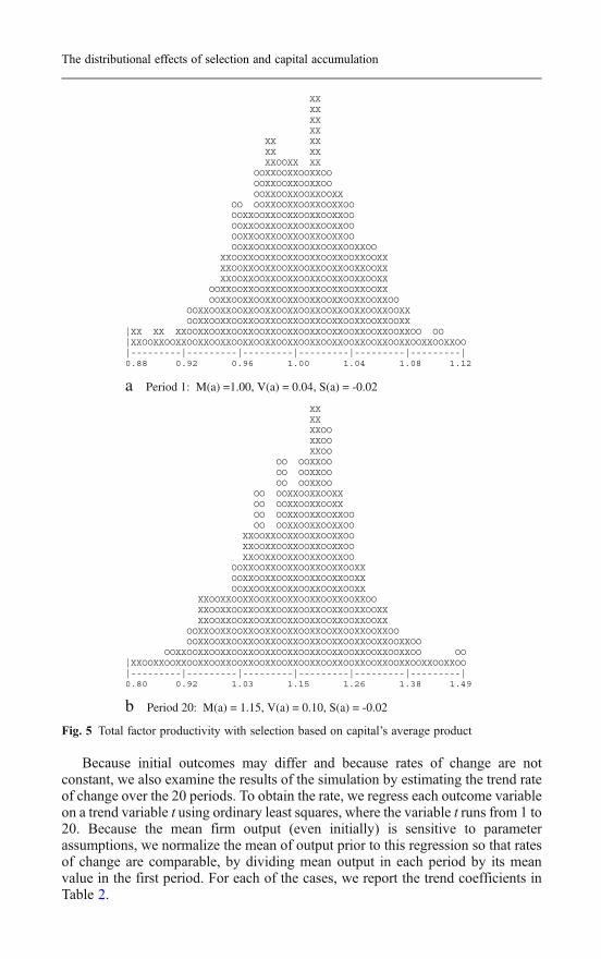
Because initial outcomes may differ and because rates of change are notconstant, we also examine the results of the simulation by estimating the trend rateof change over the 20 periods. To obtain the rate, we regress each outcome variableon a trend variable t using ordinary least squares, where the variable t runs from 1 to20. Because the mean firm output (even initially) is sensitive to parameterassumptions, we normalize the mean of output prior to this regression so that ratesof change are comparable, by dividing mean output in each period by its meanvalue in the first period. For each of the cases, we report the trend coefficients inTable 2.

XX XX XX XX XX XX XX XX XXOOXX XX OOXXOOXXOOXXOO OOXXOOXXOOXXOO OOXXOOXXOOXXOOXX OO OOXXOOXXOOXXOOXXOO OOXXOOXXOOXXOOXXOOXXOO OOXXOOXXOOXXOOXXOOXXOO OOXXOOXXOOXXOOXXOOXXOO OOXXOOXXOOXXOOXXOOXXOOXXOO XXOOXXOOXXOOXXOOXXOOXXOOXXOOXX XXOOXXOOXXOOXXOOXXOOXXOOXXOOXX XXOOXXOOXXOOXXOOXXOOXXOOXXOOXX OOXXOOXXOOXXOOXXOOXXOOXXOOXXOOXX OOXXOOXXOOXXOOXXOOXXOOXXOOXXOOXXOO OOXXOOXXOOXXOOXXOOXXOOXXOOXXOOXXOOXXOOXX OOXXOOXXOOXXOOXXOOXXOOXXOOXXOOXXOOXXOOXX |XX XX XXOOXXOOXXOOXXOOXXOOXXOOXXOOXXOOXXOOXXOOXXOO OO |XXOOXXOOXXOOXXOOXXOOXXOOXXOOXXOOXXOOXXOOXXOOXXOOXXOOXXOOXXOO |---------|---------|---------|---------|---------|---------| 0.88 0.92 0.96 1.00 1.04 1.08 1.12

a Period 1: M(a) =1.00, V(a) = 0.04, S(a) = -0.02 XX XX XXOO XXOO XXOO OO OOXXOO OO OOXXOO OO OOXXOO OO OOXXOOXXOOXX OO OOXXOOXXOOXX OO OOXXOOXXOOXXOO OO OOXXOOXXOOXXOO XXOOXXOOXXOOXXOOXXOO XXOOXXOOXXOOXXOOXXOO XXOOXXOOXXOOXXOOXXOO OOXXOOXXOOXXOOXXOOXXOOXX OOXXOOXXOOXXOOXXOOXXOOXX OOXXOOXXOOXXOOXXOOXXOOXX XXOOXXOOXXOOXXOOXXOOXXOOXXOOXXOO XXOOXXOOXXOOXXOOXXOOXXOOXXOOXXOOXX XXOOXXOOXXOOXXOOXXOOXXOOXXOOXXOOXX OOXXOOXXOOXXOOXXOOXXOOXXOOXXOOXXOOXXOO OOXXOOXXOOXXOOXXOOXXOOXXOOXXOOXXOOXXOOXXOO OOXXOOXXOOXXOOXXOOXXOOXXOOXXOOXXOOXXOOXXOOXXOO OO |XXOOXXOOXXOOXXOOXXOOXXOOXXOOXXOOXXOOXXOOXXOOXXOOXXOOXXOOXXOO |---------|---------|---------|---------|---------|---------| 0.80 0.92 1.03 1.15 1.26 1.38 1.49

b Period 20: M(a) = 1.15, V(a) = 0.10, S(a) = -0.02

Fig. 5 Total factor productivity with selection based on capital’s average product


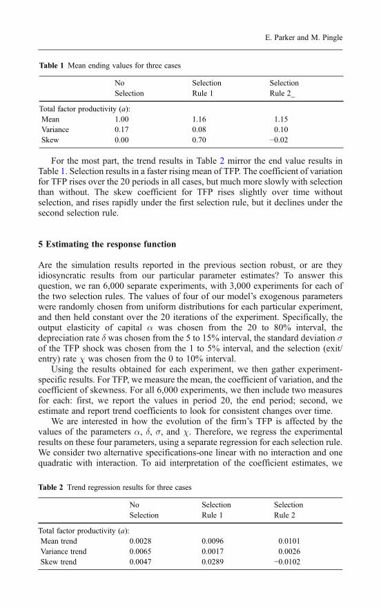
For the most part, the trend results in Table 2 mirror the end value results inTable 1. Selection results in a faster rising mean of TFP. The coefficient of variationfor TFP rises over the 20 periods in all cases, but much more slowly with selectionthan without. The skew coefficient for TFP rises slightly over time withoutselection, and rises rapidly under the first selection rule, but it declines under thesecond selection rule.

5 Estimating the response function

Are the simulation results reported in the previous section robust, or are theyidiosyncratic results from our particular parameter estimates? To answer thisquestion, we ran 6,000 separate experiments, with 3,000 experiments for each ofthe two selection rules. The values of four of our model’s exogenous parameterswere randomly chosen from uniform distributions for each particular experiment,and then held constant over the 20 iterations of the experiment. Specifically, theoutput elasticity of capital α was chosen from the 20 to 80% interval, thedepreciation rate δ was chosen from the 5 to 15% interval, the standard deviation σof the TFP shock was chosen from the 1 to 5% interval, and the selection (exit/entry) rate χ was chosen from the 0 to 10% interval.

Using the results obtained for each experiment, we then gather experiment-specific results. For TFP, we measure the mean, the coefficient of variation, and thecoefficient of skewness. For all 6,000 experiments, we then include two measuresfor each: first, we report the values in period 20, the end period; second, weestimate and report trend coefficients to look for consistent changes over time.

We are interested in how the evolution of the firm’s TFP is affected by thevalues of the parameters α, δ, σ, and χ. Therefore, we regress the experimentalresults on these four parameters, using a separate regression for each selection rule.We consider two alternative specifications-one linear with no interaction and onequadratic with interaction. To aid interpretation of the coefficient estimates, we

Table 2 Trend regression results for three cases

No Selection SelectionSelection Rule 1 Rule 2

Total factor productivity (a):Mean trend 0.0028 0.0096 0.0101Variance trend 0.0065 0.0017 0.0026Skew trend 0.0047 0.0289 −0.0102

Table 1 Mean ending values for three cases

No Selection SelectionSelection Rule 1 Rule 2_

Total factor productivity (a):Mean 1.00 1.16 1.15Variance 0.17 0.08 0.10Skew 0.00 0.70 −0.02


normalize the data prior to estimation by dividing each data point by the absolutevalue of its sample mean, so that the coefficient is equal to the elasticity at the meanof the data. We report only the estimated coefficients, not standard errors, but notewhere the t-statistics exceed the 5% (*) or 1% (**) level of statistic significance. Toaid in interpreting the regression results reported in Tables 3, 4 and 5, we also usethe (†) symbol to denote estimated coefficients (other than the constant) which arestatistically significant and consistent in end and trend value for both selectionrules, and the (!!) symbol to denote coefficients that are statistically significant andconsistent in end and trend values, but reversed in sign between the two selectionrules. We are interested in the inconsistencies between selection rules, andparticularly in the effects of selection rule 2 because it is a better proxy forprofitability.

Table 3 presents the effects of the four exogenous variables α, δ, σ, and χ on themean level of firm total factor productivity. In the linear regressions, we find that

Table 3 Simulation results for mean of total factor productivity

Selection rule 1 Selection rule 2

End Trend End Trend

Mean M(a) 1.110 0.007 1.073 0.005Linear:C (constant) 0.831** −0.920** 0.843** −0.845**

α 0.004** 0.113** 0.023** 0.377** †δ 0.001 0.012 0.002 0.017σ 0.103** 1.219** 0.082** 1.063** †χ 0.076** 0.710** 0.031** 0.192** †R2 0.91 0.94 0.79 0.81Quadratic:C 0.909** −0.044 0.953** 0.493**α −0.004 −0.084** −0.068** −0.975** †δ −0.007* −0.087** −0.003 −0.025σ 0.013** 0.190** −0.024** −0.275** !!χ 0.037** 0.367** 0.028** 0.436** †α −0.001 −0.002 0.019** 0.281**αδ 0.002* 0.046** −0.004* −0.032ασ 0.004** 0.156** 0.028** 0.491** †αχ 0.002** −0.012* 0.029** 0.339**δ 0.001 0.006 0.005* 0.042δσ 0.002* 0.032** 0.002 0.024δχ 0.001* 0.008 −0.005** −0.057**σ 0.003** 0.086** 0.014** 0.232** †σχ 0.078** 0.661** 0.048** 0.358** †χχ −0.021** −0.154** −0.035** −0.442** †R2 0.99 0.99 0.95 0.96

**The t-statistic exceeds the 1% (two-tailed) level of statistical significance*The t-statistic exceeds the 5% (two-tailed) level of statistical significance†Consistent and significant for both selection methods, in both end and trend!!Consistent and significant in both end and trend, but sign reverses with selection method


greater variation in the productivity shocks σ and higher rates of selection χ lead tofaster TFP growth under either selection rule. Changes in the depreciation rate δhave little effect on TFP under either selection rule. Under selection rule 2,increasing the output elasticity for capital α, which is the same as reducing theamount of diminishing returns, increases TFP; this is because firms with higherTFP and larger capital stocks are less likely to be selected for exit becausediminishing returns does not so quickly reduce the productivity of the large capitalstock. In the quadratic regressions, we find that the marginal effect of selection isfalling at higher selection rates, and the interaction between variation and selectionis positive. We also find one of the coefficients changes sign between the twoselection methods, but interpretation is difficult in the quadratic case.

Table 4 presents the effects of the four exogenous variables α, δ, σ, and χ on thecoefficient of variation for TFP. Greater variation in the productivity shocks leadsto greater variation in TFP, of course. However, this effect diminishes since it isnegative in its square, and it also declines with greater rates of selection. Greater

Table 4 Simulation results for variance of total factor productivity


End Trend End Trend

Mean V(a) 0.071 0.002 0.085 0.003Linear:C 0.516** 1.025** 0.518** 0.966**α −0.008 −0.014 −0.069** −0.155**δ 0.007 0.016 −0.014 −0.020σ 0.841** 0.665** 1.000** 1.029** †χ −0.435** −0.864** −0.330** −0.567** †R2 0.89 0.78 0.93 0.83Quadratic:C 0.149** 0.276** −0.045 −0.191*α 0.001 0.020 0.158** 0.414**δ 0.042 0.119 0.013 0.099σ 1.453** 1.896** 1.727** 2.453** †χ −0.520** −1.064** −0.209** −0.388** †αα −0.002 −0.006 −0.065** −0.177**αδ −0.000 −0.018 0.017 0.044ασ 0.009 0.026 −0.090** −0.206**αχ −0.009 −0.022 −0.024** −0.052**δδ −0.012 −0.031 −0.027 −0.094*δσ 0.000 −0.004 −0.028* −0.057*δχ −0.011 −0.020 0.044** 0.093**σσ −0.075** −0.156** −0.129** −0.264** †σχ −0.465** −0.929** −0.351** −0.633** †χχ 0.282** 0.579** 0.106** 0.208** †R2 0.98 0.96 0.97 0.91

**The t-statistic exceeds the 1% (two-tailed) level of statistical significance*The t-statistic exceeds the 5% (two-tailed) level of statistical significance†Consistent and significant for both selection methods, both end and trend


selection reduces the variance, but the negative effect declines as the rate ofselection rises and it rises with greater variation. A reduction in the extent ofdiminishing returns reduces the variation of TFP under selection rule 2, a result thatdoes not yet have an intuitively obvious explanation.

Table 5 presents the effects of the four exogenous variables α, δ, σ, and χ on theskew of TFP, and we find that the results are very dependent on the selection rule. Agreater selection rate leads to a more negative skew under rule 2, but a morepositive skew under rule 1. Greater variation in productivity shocks leads to a morepositive skew under selection rule 2, but a more negative skew under rule 1.Reducing the extent of diminishing returns leads to a more positive skew under rule2, but more negative skew under rule 1. Put differently, for rule 2, which is of moreinterest, a move from a more negative to more positive skew can result from alower selection rate, greater variation in the productivity shock, or a reduction inthe extent of diminishing returns.

Table 5 Simulation Results for Skew of Total Factor Productivity


End Trend End Trend

Mean S(a) 0.590 0.028 0.099 −0.002Linear:C 1.297** 1.547** 0.151** −0.029α −0.098** −0.144** 0.185** 0.221** !!δ −0.036 −0.041 0.006 0.026σ −0.111** −0.146** 0.161** 0.241** !!χ 0.501** 0.483** −0.245** −0.611** !!R2 0.40 0.27 0.18 0.28Quadratic:C 0.618** 0.745** 0.786** 1.075**α 0.116 0.161 −0.783** −1.060**δ −0.080 0.148 0.185 0.300σ 0.082 −0.139 0.055 0.148χ 1.943** 2.117** −1.044** −2.666** !!αα −0.027 −0.094 0.495** 0.712**αδ −0.042 −0.065 −0.161** −0.215*ασ −0.059 0.007 0.063 0.066αχ −0.049 −0.050 0.061* −0.025δδ 0.065 −0.042 0.043 0.070δσ −0.032 −0.018 0.023 0.000δδ −0.012 −0.020 −0.105** −0.139**σσ −0.049 −0.003 0.009 −0.013σχ −0.012 0.002 −0.002 0.046χχ −0.681** −0.778** 0.419** 1.080** !!R2 0.60 0.45 0.30 0.50

**The t-statistic exceeds the 1% (two-tailed) level of statistical significance*The t-statistic exceeds the 5% (two-tailed) level of statistical significance!!Consistent and significant for both end and trend, but sign reverses with selection method


6 Conclusion

Our model and simulations have allowed us to confirm some intuitively expectedimpacts of selection and explore impacts on skew of the firm total factorproductivity distribution that are less intuitive. Confirming the intuitive, we findthat more variable factor productivity shocks and an increased selection rateimprove TFP on average, and more variable productivity shocks increase thevariance of TFP while greater selection rates reduce the variance of TFP. Exploringthe less intuitive impact on skew, we find the effect of selection on the skewdepends upon the selection rule. When the selection criterion depends upon thefirm’s rate of return, the firms with the lowest TFP levels are not necessarily thosethat are shut down. Consequently, the distribution of TFP need not become morepositively skewed as the selection rate rises.

As they stand, our results offer an explanation for why econometricianssometimes find that firm total factor productivity distributions do not matchtheoretical expectations. It may be that, as in our simulation, the mean, variance,and skew of real world total factor productivity distributions are correlated with thecriteria that are selecting firms for exit. A positively skewed distribution of totalfactor productivity results when the selection criterion places more weight on totalfactor productivity compared to other influences, while these effects are not foundwhen the selection criterion gives weight to the return on capital, at least whendiminishing returns to capital allows smaller firms with lower total factorproductivity to catch up. Our simulations suggest econometricians should becautious about having an expectation for the skew of total factor productivitydistribution, and should consider the different roles selection and capitalaccumulation (or other factors) may play in altering skew.

References

Aigner D, Lovell CA CAK, Schmidt P (1977) Formulation and estimation of stochastic frontierproduction function models. Journal of Econometrics 6:21–37

Alchian AA (1950) Uncertainty, evolution, and economic theory. Journal of Political Economy63:211–221

Barro RJ, Sala-I-Martin X (1995) Economic Growth. McGraw-Hill, New YorkBartelsman EJ, Dhrymes P (1998) Productivity dynamics: U.S. manufacturing plants, 1972–

1986. Journal of Productivity Analysis 9:5–34Cargill TF, Parker E (2002) Asian finance and the role of bankruptcy: a model of the transition

costs of financial liberalization. Journal of Asian Economics 13:297–318Carree MA (2002) Technological inefficiency and the skewness of the error component in

stochastic frontier analysis. Economic Letters 77:101–107Cass D (1965) Optimum growth in an aggregative model of capital accumulation. Review of

Economic Studies 32:233–240Charnes A, Cooper WW, Rhodes E (1978) Measuring the efficiency of decision-making units.

European Journal of Operational Research 3:392–444Dwyer DW (1998) Technology locks, creative destruction, and non-convergence in productivity

levels. Review of Economic Dynamics 1:430–473Ericson R, Pakes A (1995) Markov-perfect industry dynamics: a framework for empirical work.

Review of Economic Studies 62:53–82Foster L, Haltiwanger J, Krizan CJ (1998) Aggregate productivity growth: Lessons from

microeconomic evidence. NBER, working paper 6803, Cambridge, MA, USAGiannakas K, Tran KC, Tzouvelekas V (2003) On the choice of functional form in stochastic

frontier modeling. Empirical Economics 28:75–100


Green A, Mayes D (1991) Technical inefficiency in manufacturing industries. Economic Journal101:523–538

Jovanovic B (1982) Selection and the evolution of industry. Econometrica 50:649–670Koopmans TC (1965) On the concept of optimal economic growth. In The Economic Approach

to Development Planning. Elsevier, AmsterdamKumbhakar SC, Orea L (2004) Efficiency measurement using a latent class stochastic frontier,

Empirical Economics 29:169–183Levinsohn J, Petrin A (1999) When industries become more productive, do firms? Investigating

productivity dynamics. NBER, working paper 6893, Cambridge, MA, USAMontgomery E, Wascher W (1988) Creative destruction and the behavior of productivity over the

business cycle. Review of Economics and Statistics 70:168–172Parker E (1995) Schumpeterian creative destruction and the growth of Chinese enterprises. China

Economic Review 6:201–223Pinker S (1997) How the mind works. W.W.Norton, New YorkRamsey FP (1928) A mathematical theory of saving. Economic Journal 38:543–559Rigby DL, Essletzbichler J (2000) Impacts of industry mix, technological change, selection and

plant entry/exit on regional productivity growth. Regional Studies 34:333–342


Elliott Parker. Mark Pingle The distributional effects of ...

Documents

Transcript of Elliott Parker. Mark Pingle The distributional effects of ...