ELK 1312 49 Manuscript 1

7/21/2019 ELK 1312 49 Manuscript 1

http://slidepdf.com/reader/full/elk-1312-49-manuscript-1 1/20

Behavior characteristic of a cap-resistor, memcapacitor and a memristor from theresponse obtained of RC and RL electrical circuits described by fractional differential

equationsJosé Francisco GÓMEZ AGUILAR*.

Department of Solar Materials, Renewable Energy Institute.National Autonomous University of Mexico.

Priv. Xochicalco s/n. Col. Centro. Temixco Morelos, Mexico.

Abstract

This paper provides an analysis of a RC and RL electrical circuits described by a fractionaldiff erential equation of Caputo type, the order considered is0 < ɣ ≤ 1. The Laplacetransform of the fractional derivative is used. To keep the dimensionality of the physicalquantities R, C and L an auxiliary parameterσ is introduced characterizing the existence offractional components in the system. The relationship betweenɣ and σ is reported. Theresponse obtained from the fractional RC and RL circuits exhibits a characteristic behaviorsof a cap-resistor, memcapacitor and memristor, as well as charge-voltage formemcapacitive systems and current-voltage for memristive systems. The relationshipbetween Ohm's law and Faraday’s laws for the charge stored in a capacitor and induction isreported. Illustrative examples are presented.

Keywords: Fractional Calculus, Mittag-Leffler Functions, Electrical Circuits, FractionalDifferential Equation, Cap-resistor, Memcapacitor, Memristor.

1 – Introduction

The application of Fractional Calculus (FC) has the attracted interest of researchers inrecent decades. FC is the generalization of ordinary integrals and derivatives of integerorders to arbitrary orders, this topic is nearly as old as conventional calculus, however,these ideas seem to be quite a sophisticated topic and are not very easy to explain, mainlydue to the lack of relation to some common important physical concepts, such as velocity

and acceleration. We provide examples from many areas of physics; engineering andbioengineering based on derivatives of non-integer order (see references. [1-8] and thereferences therein). FC provides an excellent instrument for the description of hereditaryproperties of various materials and processes. In comparison with the classical integer-ordermodels the FC provides effects not considered, this is its main advantage.

Modeling as fractional order proves to be useful particularly for systems wherememory or hereditary properties play a signicant role. This is due to the fact that aninteger order derivative at a given instant is a local operator which considers the nature ofthe function at that instant and within its neighborhood only, whereas a fractional derivative

7/21/2019 ELK 1312 49 Manuscript 1


takes into account the past history of the function from an earlier point in time, called“lower terminal” up to the instant at which the derivative is to be computed. Fractional

order models have already been used for modeling of electrical circuits (such as dominoladders, tree structures, etc.) and elements (coils, memristor, etc.) [9-10]. Unlike the workof the authors mentioned above, in which there is a direct passing from an ordinaryderivative to a fractional one, here first we analyze the ordinary derivative operator andthen try to bring it to the fractional form in a consistent manner.

The aim of this work is the generalization of RC and RL electrical circuits usingfractional differential equations, the generalization of these circuits yielded characteristicbehaviors of a cap-resistor, a memcapacitor and a memristor. This paper is organized asfollows. Section two briefly reviews elements with memory: cap-resistor, memcapacitor,

meminductor and memristor. Section three presents the basic definitions of fractionalcalculus. Section four looks at the construction of fractional differential equations. The fifthsection analyzes fractional relations in main passive elements. Section six presentsapplication examples and finally, the seventh section is devoted to our conclusions.

2 – Elements with Memory

Traditionally electrical circuit theory has been developed considering three basic elements:resistance, capacitors and inductors. Leon Chua in 1970 found, from a mathematical pointof view, symmetry principles between the four electrical variables of a circuit: currenti,voltagev, chargeq and magnetic fluxψ . Chua predicted the existence of a missing element,the memristor (short for memory resistor) M , M = d ψ /dq , this element describes therelationship between the magnetic flux and charge. A memristor is a resistor that changesits resistance depending on the magnitude and direction of the current going through it, thisdevice has the property of conserving resistance even with an interrupted or eliminatedcurrent flow. This memory capacity gives the memristor ample possibilities of anapplication in the manufacture of non-volatile memories with a higher integration densitythan current ones [11]. This device has captured the interest of the scientific communitydue to its capacity to function in an analog way as would happen in synapse in the humanbrain; it is considered that its multiple applications will give rise to a technological

revolution similar to the one produced by transistors in its moment [12]. In April 2008 theStanley Williams research group working in Hewlett-Packard laboratories announced thephysical realization of the memristor, which behaved as predicted by Chua in 1970 [13].The cap-resistor was proposed by Reyes-Melo [14], this fractional element defines the

intermediate behavior between a resistor and a capacitor,( ) , RC d qC dt

vγ γ

γ = where C is thecapacitance, R the resistance,q the charge and0 < ɣ ≤ 1. This device displays a similarbehavior to the Constant Phase Element (CPE) which is commonly used as way to correctthe deviation from ideal capacitors and for characterizing the electrochemical properties ofbiological tissues and biochemical materials [15]. Some authors [16] present differential

7/21/2019 ELK 1312 49 Manuscript 1


and integral operators of fractional order in the modeling of relaxation phenomena in semi-crystalline polymers; the cap-resistor describes the viscoelastic behavior of certain

polymeric systems. The memcapacitor offers a link between time integral of chargeq andflux ψ , qdt ψ = ∫ and the meminductor links chargeq with the time integral of the flux

ψ , ,q dt ψ = ∫ namely capacitors and inductors whose capacitance and inductance,respectively, depend on past states. Various systems exhibit memcapacitive ormeminductive behavior including vanadium dioxide metamaterials, nanoscale capacitorswith interface traps, or embedded nanocrystals [17–18]. The theory of mem-elements hasbeen extensively reviewed [19-23].

3 – Overview of Fractional Calculus

The definitions of fractional order derivatives are not unique and several, including:Riemann-Liouville, Grünwald-Letnikov and the Caputo Fractional Derivative (CFD). In theCaputo case, the derivative of a constant is zero and the initial conditions for the fractionaldifferential equations have a known physical interpretation. For function f(t), CFD isdefined as [4]

( )

10

1 ( )( ) ,( ) ( )

nt C o t n

f D f t d

n t γ

γ

τ τ

γ τ − +=Γ − −

∫ (1)

wheren = 1, 2 , … , ɛ N andn – 1 < ɣ ≤ n. We consider the casen = 1 , i.e., in the integrandthere is only a first derivative. In this case, 0 <ɣ ≤ 1, is the order of the fractionalderivative.

For example, in the case f(t) = t k , wherek is an arbitrary number and 0 <ɣ ≤ 1 wehave the following expression for the CFD

0( ) , (0 1),

( 1 )C k k

t

k k D t t

k γ γ γ

γ −Γ

= < ≤Γ + −

(2)

whereГ is the gamma function. Ifɣ = 1, the expression (2) yields the ordinary derivative.

1 10 .

k C k k

t

dt D t kt

dt −= = (3)

The Laplace transform to CFD is given by [4]

11 ( )

0( ) ( ) (0).

mC k k o t

k

L D f t S F s S f γ γ γ −

− −

=

= − ∑ (4)

7/21/2019 ELK 1312 49 Manuscript 1


The Mittag-Leffler function has caused extensive interest among physicists due toits vast potential for applications describing realistic physical systems with memory and

delay. The Mittag-Leffler function is defined by

0( ) , ( 0),

( 1)

m

am

t E t a

am

∞

=

= >Γ +

∑ (5)

whena = 1 , from (5), we obtain

10 0

( ) ,( 1) !

m mt

m m

t t E t e

m m

∞ ∞

= =

= = =Γ +

∑ ∑ (6)

where the exponential function is a particular case of the Mittag-Leffler function.

4 – Construction of Fractional Differential Equations, an Alternative

Some authors replace the integer derivative with a fractional one on a purely mathematicalbasis. However, from the physical and engineering point of view this is not completelycorrect because the physical parameters contained in the differential equation should nothave the dimensionality measured in the laboratory. One possible way to clarify thesethings is to replace the ordinary time derivative operator with the fractional one in thefollowing way

, 0 1d d dt dt

γ

γ γ → < ≤ (7)

It can be seen that equation (7) is not quite right from a physical point of viewbecause the time derivative operatord/dt has a dimension of inverse seconds s-1, while thefractional time derivative operatord ɣ /dt ɣ has, s-ɣ. To be consistent with the timedimensionality we propose the use of a new parameterσ in the following way,

111 , 0 1d sdt

γ

γ γ γ σ −

= < ≤ (8)

whereɣ is an arbitrary parameter which represents the order of the derivative. In the caseɣ = 1 the expression (8) becomes an ordinary derivative operator. In this way (8) isdimensionally consistent if, and only if, the new parameterσ , has a dimension of time [σ ] =s. This time is called the cosmic time [24] and is a non-local time. Another physical andgeometrical interpretation of the fractional operators is given [25]. The fractional operatoris defined by

11 , -1d d n n

dt dt γ

γ γ γ σ −→ < ≤ (9)

7/21/2019 ELK 1312 49 Manuscript 1


The expression (9) is a time derivative because its dimension iss-1. The parameterσ (auxiliary parameter) represents the fractional time components, this components shows an

intermediate behavior between a conservative and a dissipative system.5 – Fractional Relations in Main Passive Elements.

Ohm’s law states that the current flowing through a conductor between two given points isdirectly proportional to the potential difference as well as inversely proportional to theresistance between them. The mathematical formula can be written as follows

( ) ( ),v t Ri t = (10)

wherei(t) is the current flowing through the conductor measured in Ampers(A), v(t) is the

potential difference measured between two points of the conductor with units of VoltsVand R is the resistance of the conductor measured in Ohms. The current is the change inthe chargeq with respect to timet, this current is defined by

( ) .dqi t dt = (11)

Taking this into account, Ohm’s law can be written as a function of the chargeq(t) ,

( ) .dqv t R dt = (12)

The idea is to rewrite Ohm’s law in terms of fractional derivative. Using theexpression (9), Ohm’s law (12) becomes a fractional Ohm’s law

1( ) , n-1 ,d q Rv t ndt

γ

γ γ γ σ −= ≤ ≤ (13)

whenn = 1 andγ = 1 from the expression (13) we have (12).

As this new parameterσ , has the dimension of time [σ ] = s. There are two possiblecases relating to this parameter, the first relates to an RC circuit where the productσ = RC is the time constant of an RC circuit and its dimensions are seconds, while the other case iswhenσ = L/R which representing the time constant of an RL circuit and its dimensions alsoin seconds.

First case: Ifσ = RC andn = 1 of (13)

1( ) , 0 1,( )d q Rv t

RC dt

γ

γ γ γ −= ≤ ≤ (14)

whenγ = 1 the expression (14) becomes (12). Whenγ = 0 the expression (14) is

7/21/2019 ELK 1312 49 Manuscript 1


( ) .qv t C = (15)

Equation (15) is the Faraday law for the charge stored in a capacitor.Second case: Ifσ = L/R andn = 2 of (13)

( )1( ) , 1 2.d q Rv t

dt L R

γ

γ γ γ −= ≤ ≤ (16)

The derivative of (16) with respect to time is

( )1

1

1 ( )( ) , 1 2,d i t Lv t R R dt

γ

γ

γ γ

−

−

−= ≤ ≤ (17)

wherei(t) is the current, if β = ɣ – 1 in (17) we obtain

( ) ( )( ) , 0 1,d i t Lv t R R dt

β β

β β = ≤ ≤ (18)

when β = 1 the expression (18) is

( )( ) .di t v t L dt = (19)

Equation (18) is the Faraday law of induction. When β = 0 the expression (18)becomes (10). Equations (15) and (19) show the existence of capacitive and inductiveproperties in the resistance. The following section describes the RC and RL electricalcircuits using fractional differential equations.

6 – Application Examples

6.1 – Fractional RC Circuit

Below, a fractional RC circuit and its generalization are described

The RC circuit is represented in Figure 1; applying Kirchhoff’s law the fractionaldifferential equation for the RC circuit has the form

1 ( ) ( ),d q C q t v t dt

γ

γ γ γ

τ τ + = (20)

where

1 , 0 1. RC γ γ τ γ σ −= < ≤ (21)

7/21/2019 ELK 1312 49 Manuscript 1


Equation (21) can be called a fractional time constant due to its dimensionalitysγ.Whenγ = 1, in (21) we obtain the ordinary time constant,τ = RC . Assume thatq(0) = 0 for

any timet , v(t) = V ou(t), where V o is a constant source of voltage andu(t) is the stepfunction. Applying Laplace transform in (20) with zero initial conditions we have

0( ) .1

CV Q s

s s γ γ

γ τ τ

= +

(22)

Applying the inverse Laplace transform in (22) we obtain the behavior of the chargerespect to time t

1

0( ) 1 ,q t CV E t RC

γ γ

γ σ −

= − − (23)

where E γ(t) is the Mittag-Leffler function.

The parameterγ, which represents the order of the fractional differential equation(20), can be related to the parameterσ , which characterizes the presence of fractionalcomponents in the system. In this case the relationship is given by the expression

, RC σ γ = (24)

If γ = 1 , then, from (24)σ = RC , which means that there are no fractional components inthe system, that is to say, it is a regular RC . However, in the range 0 <γ < 1, or theequivalent0 < σ < RC, fractional structures are present in the system.

Substituting the expression (24) in (23) we have

( )}{ 10 ˆ( ) 1 ,q t CV E t γ γ

γ γ −= − − (25)

where ˆ ,t t RC = is a dimensionless parameter. From (25), we obtain the voltage across the

capacitor

( )}{ 10 ˆ( ) 1 .v t V E t γ γ

γ γ −= − − (26)

The current is ( )( ) dq t i t dt = , then from (25) we obtain

( )}{ 10 ˆ( ) 1 .ˆV d i t E t R dt

γ γ γ γ −= − − (27)

7/21/2019 ELK 1312 49 Manuscript 1


Given the values, R = 1 M , C = 1 µF , we simulate equations (25), (26) and (27),obtaining Figure 2 and Figure 3, which show the behavior of the charge and voltage across

the capacitor (in the same Figure) and the current across the resistance, respectively.Intermediate values between0 1γ < ≤ indicate the existence of another capacitive

element different from the ideal capacitor in the RC circuit shown in Figure 1. Fractionalstructures (components that show an intermediate behavior between a system conservative(capacitor) and dissipative (resistor)) are presented; this behavior indicate the existence ofthe cap-resistor element.

Now assuming thatq(0) = a , wherea is a constant defined in the range( ; ).−∞ ∞ For any timet , v(t) = V ou(t), whereV o is a constant source of voltage andu(t) is the step

function. Applying Laplace transform in (20) we obtain0( ) .11

CV aQ s

ss s γ γ

γ γ γ τ τ τ

= ± ++

(28)

Applying the inverse Laplace transform in (28) we obtain the behavior of the chargerespect to time t

( )}{ ( ){ }1 1 10 ,ˆ ˆ( ) 1 ,q t CV E t a t E t γ γ γ γ γ

γ γ γ γ γ − − −= − − ± − (29)

where E γ(t) and E γ ,γ (t) are the Mittag-Leffler functions, andˆ ,t t RC = is a dimensionless

parameter.

From (29), we obtain the voltage across the capacitor

( )}{ ( ){ }1 1 10 ,ˆ ˆ( ) 1 .a

v t V E t t E t C

γ γ γ γ γ γ γ γ γ γ − − −= − − ± − (30)

The current is ( )( ) dq t i t dt = , then from (29) we obtain

}{ ( ){ }1 1 10 0,ˆ ˆ( ) 1 .ˆ ˆ

V d aV d i t E t t E t R RC dt dt γ γ γ γ γ

γ γ γ γ γ − − − = − − ± − (31)

If a=0 , in (29), (30) and (31) we obtain equations (25), (26) and (27) respectively.For example, given values R = 1 M , C = 1 µF anda = -0.01 , we simulate equations (29),(30) and (31) obtaining Figure 4 and Figure 5 which show the behavior of the charge andvoltage across the capacitor (in the same figure) and the current across the resistance,respectively.

7/21/2019 ELK 1312 49 Manuscript 1


Given the values, R = 0.01 M , C = 1 µF anda = 0.01 , we simulate equations (29),(30) and (31) obtaining Figure 6 and Figure 7, which show the behavior of the charge and

voltage across the capacitor (in the same figure) and the current across the resistance,respectively.

If the source in equations (25), (26), and (27) isv(t) = V , whereV = sin( ω t), ω =2π 60, we obtain Figures 8 and 9 for the behavior of the charge and voltage across thecapacitor (in the same figure) and the current across the resistance, respectively.

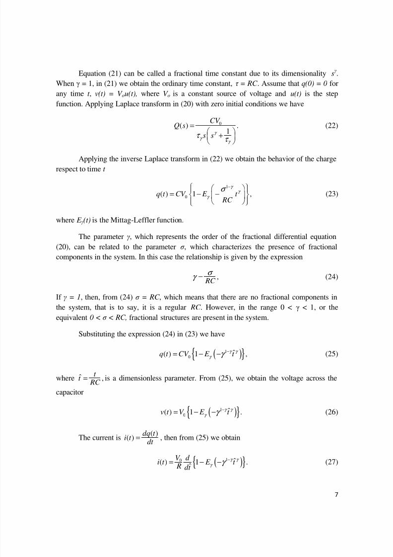
Figure 10 shows the hysteresis curve for the cap-resistor element, this curve exhibita memcapacitive behavior (memory capacitance). After the transient, in the steady-state thecircuit behaves as a memcapacitor.

5.2 – Fractional RL Circuit

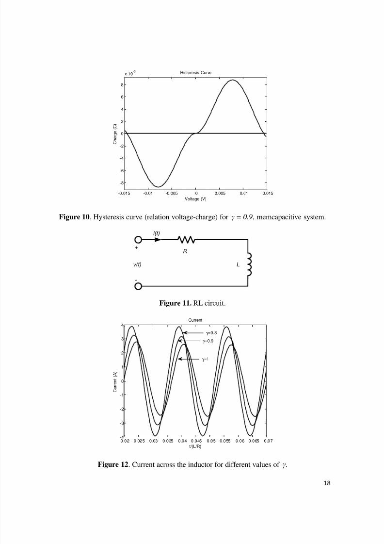
The RL circuit is represented in Figure 11. R is the resistance, L is the inductance,and v(t) is the voltage source. The fractional differential equation for the RL circuit has theform

1( ) 1( ) ( ),d i t i t v t Rdt

γ

γ γ γ

τ τ + = (32)

where

1 , 0 1 L R

γ γ τ γ σ −= < ≤ (33)

it can be called a fractional time constant due to its dimensionalitysɣ . Whenγ = 1 , from

(33) we obtain the well-known time constant L R

τ = . We assume thati(0) = 0 and for any

time t , v(t) = V , whereV = sin( ω t), ω = 2 π 60 . Applying Laplace transform in (32) withzero initial conditions, we obtain

( )1( ) ( ) ,

V ss I s I s R

γ

γ γ τ τ + = (34)

solving for I(s), we obtain

( )( ) , 0 1.1

V s I s

R s γ γ

γ

γ τ τ

= < ≤ +

(35)

7/21/2019 ELK 1312 49 Manuscript 1


7/21/2019 ELK 1312 49 Manuscript 1


In the special case where the initial condition is zero for the charge and current, theRC and RL circuits behave as a memcapacitor and memristor element in steady-state and it

has a zero-crossing hysteresis loop, charge-voltage for memcapacitive systems and current-voltage for memristive systems.

The generalized RC circuit (in the range0 1γ < ≤ ) exhibits a behavior similar to thecap-resistor that can be used as an equivalent circuit in the modeling of processes in whichthe behavior of the systems show competition between a resistive and capacitive element.For example biological systems or polymeric systems, on the other hand the generalized RLcircuit (in the range1 2γ < ≤ ) exhibits a behavior similar to the memristor and can be usedas an equivalent circuit in the modeling of processes in which the behavior of the systemsshow competition between a resistive and inductive element.

Equations (29), (30) and (31) represent the fractional equations for the charge,voltage, and current in the RC circuit, respectively, and provide the generalization of theelectrical circuits; equation (24) characterizes the existence of the fractional structures inthe system. The fractional components change the time constant and affect the transientresponse of the system. We also found that there is a relation betweenɣ and σ , dependingon the system studied. Equation (35) represents the fractional equation for the current in theRL circuit; the numerical Laplace transform method was used for the simulation ofequations for the current and voltage.

A meminductor and a memcapacitor behave in the same fashion as a memristor; fora meminductor hysteresis curve (current-flow) there would be various current-flowrelationships. The meminductor behaves as an inductance because for every magnetic flowvalue we obtain a current value, but to determine this we need to know the memory of thedevice; in the case of the memcapacitor hysteresis curve (charge-flow) we would obtainvarious charge-flow relationships, with this behavior stemming from the memory effect.

With the approach here presented it will be possible to better study of transienteffects in electrical systems. The electrical circuit will provide a robust framework forstudying the bioelectrical response to transient stimuli, when an equivalent electrical circuithas been used; also, we have extended fractional calculus to the study of electrical circuitsand the notion of memory devices to both capacitive and inductive systems described forelectrical circuits RC and RL.

Acknowledgments

The author acknowledges fruitful discussions with Mayra Martínez. This work wassupported by CONACYT.

References

7/21/2019 ELK 1312 49 Manuscript 1


[1] H. Nasrolahpour, “Time fractional formalism: classical and quantum phenomena”.Prespacetime Journal, Vol. 3, pp. 99-108, 2012.

[2] K.B. Oldham, J. Spanier, “The fractional calculus”, Academic Press, New York, 1974.

[3] K.S. Miller, B. Ross, “An introduction to the fractional calculus and fractionaldifferential equations”, Wiley, New York, 1993.

[4] I. Podlubny, “Fractional differential equations”, Academic Press, New York, 1999.

[5] R. Hilfer, “Applications of fractional calculus in physics”, World Scientific, Singapore,2000.

[6] J.J. Rosales, M. Guía, J.F. Gómez, V.I. Tkach, “Fractional electromagnetic wave”,Discontinuity, Nonlinearity and Complexity, Vol. 1, pp. 325-335, 2012.

[7] R.L. Magin, “Fractional calculus in bioengineering”, Begell House Publisher, Rodding,2006.

[8] D. Baleanu, Z.B. Günvenc, J.A. Tenreiro Machado, “New trends in nanotechnology andfractional calculus applications”, Springer, 2010.

[9] A. Obeidat, M. Gharibeh, M. Al-Ali, A. Rousan. “Evolution of a current in a resistor”.Fract. Calc. App. Anal. 14, 2, Springer, 2011.

[10] I. Petras. “Fractional-Order Memristor-Based Chua's Circuit”. IEEE Transactions onCircuits and Systems-II: Express Briefs. 57, 12, 2010.

[11] Gorm K. Johnsen. “An introduction to the memristor – a valuable circuit element inbioelectricity and bioimpedance”. Journal of Electrical Bioimpedance, Vol. 3, pp. 20–28,2012.

[12] V.M. Jimenez-Fernandez, J.A. Dominguez-Chavez, H. Vazquez-Leal, A. Gallardo delAngel, Z.J. Hernandez-Paxtian. “Descripción del modelo eléctrico del memristor”. RevistaMexicana de Física E 58, pp. 113–119, 2012.

[13] Oliver Pabst, Torsten Schmidt. “Frequency dependent rectier memristor bridge usedas a programmable synaptic membrane voltage generator”. Journal of ElectricalBioimpedance, Vol. 4, pp. 23–32, 2013.

[14] M.E. Reyes-Melo, J.J. Martinez-Vega, C.A. Guerrero-Salazar and U. Ortiz-Mendez.“Application of fractional calculus to modeling of relaxation phenomena of organic

7/21/2019 ELK 1312 49 Manuscript 1


dielectric materials”, Proceedings IEEE International Conference Solids Dielectrics, pp.530-533, 2004.

[15] F. Gómez, J. Bernal, J. Rosales and T. Córdova, “Modeling and simulation ofequivalent circuits in description of biological systems - a fractional calculus approach”,Journal of Electrical Bioimpedance, Vol. 3, pp 2-11, 2012.

[16] M.E. Reyes-Melo, J.J. Martinez-Vega, C.A. Guerrero-Salazar, U. Ortiz-Mendez.“Modelling of relaxation phenomena in organic dielectric materials. application ofdifferential and integral operators of fractional order”. Journal of Optoelectronics andAdvanced Materials, Vol. 6, pp. 1037–1043, 2004.

[17] T. Driscoll, H.T. Kim, B.G. Chae, B.J. Kim, Y.W. Lee, N.M. Jokerst, S. Palit, D.R.Smith, M. Di Ventra, D.N. Basov, Science 325, 1518, 2009.

[18] M. Di Ventra. “Electrical Transport in Nanoscale Systems”. Cambridge UniversityPress, 2008.

[19] M. Di Ventra, Y. Pershin, L. Chua. “Circuit elements with memory: memristors,memcapacitors, and meminductors”. Proc. IEEE 97, pp. 1717–1724, 2009.

[20] M.E. Fouda, A.G. Radwan, K.N. Salama. “Effect of boundary on controlledmemristor-based oscillator”. Proceedings of International Conference on Engineering andTechnology, pp. 1–5, 2012.[21] S. Jo, T. Chang, I. Ebong, B. Bhadviya, P. Mazumder, W. Lu. “Nanoscale memristordevice as synapse in neuromorphic systems”. Nano Lett. 10, pp. 1297–1301, 2010.

[22] Massimiliano Di Ventra, Yuriy V. Pershin, and Leon O. Chua. “Circuit elements withmemory: memristors, memcapacitors and meminductors”. Proceedings of the IEEE, Vol.97, 2009.

[23] Yuriy V. Pershin and Massimiliano Di Ventra. “Memristive circuits simulatememcapacitors and meminductors”. Proceedings of the IEEE, Vol. 97, 2009.

[24] I. Podlubny. “Geometric and physical interpretation of fractional integration andfractional differentiation”. Fractional Calculus and Applied Analysis, Vol. 5, pp. 367-386,2002.

[25] M. Moshre-Torbati, J.K. Hammond. “Physical and geometrical interpretation offractional operators”. Journal of the Franklin Institute, 335B , pp. 1077-1086, 1998.

7/21/2019 ELK 1312 49 Manuscript 1


Figure 1. RC circuit.

0 0.5 1 1.5 2 2.5 3 3.5 40

0.5

1x 10

-6 Charge across the Capacitor

t/RC

C h a r g e

( C )

0 0.5 1 1.5 2 2.5 3 3.5 40

0.5

1Voltage across the Capacitor

V o

l t a g e

( V )

t/RC

γ =1

γ =1γ =0.75

γ =0.75γ =0.5

γ =0.5 γ =0.25

γ =0.25

Figure 2 . Figure A) Charge across the capacitor and Figure B) Voltage across the

capacitor, both for different values ofɣ .

0 0.5 1 1.5 2 2.5 3 3.5 40

0.1

0.2

0.3

0.4

0.5

0.6

0.7

0.8

0.9

1x 10

-6 Current across the Resistor

t/RC

C u r r e n

t ( A )

γ =1

γ =0.75

γ =0.5

γ =0.25

7/21/2019 ELK 1312 49 Manuscript 1


Figure 3. Current across the resistor for different values ofγ.

0 0.5 1 1.5 2 2.5 3 3.5 4-10

0

-10-2

-10-4

Charge across the Capacitor

t/RC

C h a r g e

( C )

0 0.5 1 1.5 2 2.5 3 3.5 4-10

6

-104

-102

Voltage across the Capacitor

V o

l t a g e

( V )

t/RC

γ =0.25

γ =0.25 γ =0.5

γ =0.5

γ =0.75

γ =0.75

γ =1

γ =1

Figure 4 . Figure A) Charge across the capacitor and Figure B) Voltage across thecapacitor, both for different values ofɣ .

0 0.5 1 1.5 2 2.5 3 3.5 410

-6

10-5

10-4

10-3

10-2

10-1

100

101

Current across the Resistor

t/RC

C u r r e n

t ( A )

γ =1

γ =0.75

γ =0.5

γ =0.25


7/21/2019 ELK 1312 49 Manuscript 1


0 0.5 1 1.5 2 2.5 3 3.5 4

10 -2

Charge across the Capacitor

t/RC

C h a r g e

( C

)

0 0.5 1 1.5 2 2.5 3 3.5 4102

103

104

105


V o

l t a g e

( V )

t/RC

γ =1

γ =1

γ =0.75

γ =0.75

γ =0.5

γ =0.5

γ =0.25

γ =0.25


0 0.05 0.1 0.15 0.2 0.25 0.3-4.5

-4

-3.5

-3

-2.5

-2

-1.5

-1

-0.5

0

0.5Current across the Resistor

t/RC

C u r r e n

t ( A )

γ =0.75 γ =1

γ =0.25

γ =0.5


7/21/2019 ELK 1312 49 Manuscript 1


0 0.005 0.01 0.015 0.02 0. 025 0. 03 0. 035 0. 04 0.045

-2

-1

0

1

2

x 10-7 Charge across the Capacitor

t/RC

C h a r g e

( C

)

0 0.005 0.01 0.015 0.02 0. 025 0. 03 0. 035 0. 04 0.045

-0.2

-0.1

0

0.1

0.2


V o

l t a g e

( V )

t/RC

γ =0.25γ =0.5

γ =0.5 γ =0.25

γ =0.75

γ =0.75

γ =1

γ =1


0 0.005 0.01 0.015 0.02 0. 025 0. 03 0. 035 0. 04 0.045-8

-6

-4

-2

0

2

4

6

x 10-5 Current across the Resistor

t/RC

C u r r e n

t ( A )

γ =0.25

γ =0.5

γ =0.75

γ =1


7/21/2019 ELK 1312 49 Manuscript 1


-0.015 -0.01 -0.005 0 0.005 0.01 0.015

-8

-6

-4

-2

0

2

4

6

8

x 10-3 Histeresis Curve

Voltage (V)

C h a r g e

( C )

Figure 10 . Hysteresis curve (relation voltage-charge) forγ = 0.9 , memcapacitive system.

R

Lv(t)

+

-

i(t)

Figure 11. RL circuit.

0.02 0.025 0.03 0.035 0.04 0.045 0.05 0.055 0.06 0.065 0.07-4

-3

-2

-1

0

1

2

3

4Current

t/(L/R)

C u r r e n

t ( A )

γ =0.8

γ =0.9

γ =1

Figure 12 . Current across the inductor for different values ofγ.

7/21/2019 ELK 1312 49 Manuscript 1


0.02 0.025 0.03 0.035 0.04 0.045 0.05 0.055 0.06 0.065 0.07-15

-10

-5

0

5

10

15Voltage

t/(L/R)

V o

l t a g e

( V )

γ =0.8

γ =0.9

γ =1

Figure 13 . Voltage across the inductor for different values ofγ.

-6 -4 -2 0 2 4 6

x 10-3

-6

-4

-2

0

2

4

6Histeresis Curve

Voltage (V)

C u r r e n

t ( A )

Figure 14 . Hysteresis curve (relation voltage-current) forγ = 0.9 , memristive system.

7/21/2019 ELK 1312 49 Manuscript 1


0 0.005 0.01 0.015-1

-0.5

0

0.5

1

1.5

2Current

t/(L/R)

C u r r e n

t ( A )

γ =1

γ =1.7

γ =1.2

γ =1.4

Figure 15 . Behavior of the current for different values ofγ.

0 0.005 0.01 0.015-2

0

2

4

6

8

10x 10

-3 Charge

t/(L/R)

C h a r g e

( C )

γ =1.2γ =1.4

γ =1

γ =1.7

Figure 16 . Behavior of the charge for different values ofγ.

ELK 1312 49 Manuscript 1

Documents

Transcript of ELK 1312 49 Manuscript 1