1

Eliminating the Flaws in New England’s Reserve Markets

Peter Cramton and Jeffrey Lien1 March 2, 2000

New England’s wholesale electricity market has been in operation, since May 1, 1999. When the

market began it was understood that the rules were not perfect (Cramton and Wilson 1998). However, it

was decided that it was better to start the market with imperfect rules, rather than postpone the market for

an indefinite period. After several months of operation, we now have a sense of the extent market

imperfections have resulted in observed problems. Here we study the three reserve markets—ten-minute

spinning reserve (TMSR), ten-minute non-spinning reserve (TMNSR), and thirty-minute operating

reserve (TMOR); we also discuss the closely related operable capability (OpCap) market. The paper

covers the first four months of operation from May 1 to August 31, 1999. It is based on the market rules

and their implementation by the ISO, and the market data during this period, including bidding, operating,

and settlement information. Since that data are confidential, we have presented only aggregate

information in the tables and figures that follow.2 Although this paper will cover only the reserves

markets, we have studied the data from the energy, AGC, and capacity markets as well. Since all of the

NEPOOL markets are interrelated, one cannot hope to understand one market without having an

understanding of the others.

In this paper, we hope to accomplish four tasks:

1. Identify the potential market flaws with these markets.

2. Look at the performance of the markets to see if the potential problems have materialized.

3. Evaluate the ISO’s short-term remedies for these market flaws.

4. Propose alternative medium-term solutions to the identified problems.

1 Professor of Economics and PhD Candidate, respectively, University of Maryland, College Park MD 20742. The views expressed are our own. Please send comments to cramton@umd.edu or lien@econ.umd.edu. We are grateful to Hung-Po Chao, Alvin Klevorick, Robert Wilson, ISO New England, and numerous NEPOOL participants for helpful comments. We thank ISO New England and the National Science Foundation for funding this research. 2 When particular bidders or units are discussed it is by a bidder or unit number that we have created. No cross-reference to an actual bidder or unit ID or name is provided.

2

We conclude that the reserve markets are seriously flawed. Looking at the data, one might argue that

most of the time these markets are working well; that is, prices are “reasonable” most of the time. But this

is simply a reflection that most of the time these markets are irrelevant—most of the time the resources

these markets price are not scarce. In the absence of scarcity, the markets are doing a reasonable job of

pricing and assignment. But this is similar to an air conditioner working well in the winter. It works well,

simply because it is not asked to do anything. Like an air conditioner, the reserve markets should be

evaluated when they are stressed—when the markets are actually resolving a problem of scarcity. On this

score, the markets have performed poorly (although better than the early months in some other markets,

such as California).

The poor performance of these markets is not a surprise. It is the result of basic market flaws. These

flaws have been recognized by the ISO and NEPOOL participants, since well before the markets began

operation. Unfortunately, there was insufficient time to fix these markets before operations began on May

1, 1999. It was felt that the ISO would be able to introduce short-term fixes as needed in the early months

of operation. This has worked reasonably well. The flaws have not been fatal. The ISO has been able to

operate a workably-efficient and reliable wholesale electricity market. Indeed, it is remarkable how well

the markets have worked, despite their flaws. One measure of this is that the cost of reserves is still a

small percentage of total energy costs.3

Ideally, what is needed is a long-term fix to the basic design flaws in the reserve markets.

NEPOOL’s Congestion Management and Multi-settlement Committee is in the process of developing a

long-term solution. Realistically, it will not be possible to implement the long-term solution until late in

the year 2000, at best. In the mean time, it is worthwhile to identify a medium-term fix that the ISO can

implement within a matter of months. We present such a medium-term solution below.

Recommendation: Eliminate the OpCap market.

Given the nature of the market flaws and the difficulties of implementing more than a modest

variation of the status quo, we believe the best approach is to eliminate the OpCap market. It is hard to

argue that the OpCap market serves any useful purpose as presently designed. Since its operation has real

3 In July, the worst of the four-month period, reserves were 3.6% of the total energy bill. In contrast, in California’s first summer of operation, prices in the reserve markets were often chaotic and often substantially above energy prices. California’s ancillary service costs in July 1998 averaged $21/MWh, when energy prices averaged $32/MWh. California’s ancillary service cost before market-based rates averaged just over $1/MWh.

3

costs with no apparent gain, it is best to eliminate the market. (The ISO has taken our advice and

eliminated the market as of March 1, 2000).

Recommendation: Adopt the smart buyer model for the reserve markets.

We recommend that the reserve markets continue in the medium-term, but with the ISO adopting a

smart buyer model for reserves.4 As a smart buyer, the ISO:

1. Never pays for additional reserves more than the economic value of the additional reserves.

2. Reduces its demand for reserves as reserve prices increase.

3. Shifts purchases toward higher quality reserves when they are priced less than lower quality reserves.

In conducting the markets for reserves, the ISO is effectively purchasing reliability on behalf of load. The

ISO has a responsibility to purchase wisely, given the aggregate preferences of load. On this basis, the

ISO as smart buyer develops a demand curve for reserves that reflects the marginal value that additional

reserves have for the system.

The essential elements of the smart buyer model can be adopted in the medium-term. The ISO

recently has implemented point 3 above. The reserves now are treated as a cascade with the ISO filling its

need for lower quality reserves with higher quality reserves if the higher quality can be purchased at a

lower price. The difficult step is establishing a demand curve for reserves, which reflects the marginal

value of additional reserves. This will accomplish point 1. Point 2 is accomplished by integrating the

demand curve with the unit commitment and dispatch programs. It will require some discussion among

participants and regulators, but once new operating procedures are established the ISO can begin

purchasing reserves according to its demand curve, rather than the current vertical “demand” curve, which

does not reflect the marginal value of additional reserves. Details of how this might work are discussed in

Section 4.

Recommendation: Restructure the reserve markets.

The basic flaws in the reserve markets stem from two features of the current markets:

1. The vertical “demand” curve, derived from a rigid reserve requirement, implies that prices are

arbitrarily high in times of scarcity.

4

2. Losing bidders face the same obligations as winning bidders.

The first flaw is eliminated by constructing the true demand curve for reserves, based on the

marginal value of additional reserves. The second flaw is solved by paying everyone that provides

reserves in real time the market clearing reserve price. The real time supply curve is calculated by the ISO

based on the state of the system. The supply corresponds to the quantity of reserves that is available in the

system. The clearing price is then found at the intersection of this vertical supply curve with the demand

curve for reserves. All units providing reserves are paid this clearing price.

Recommendation: Create multi-settlement energy and reserve markets as soon as possible.

In the long term, the reserve markets should be restructured. NEPOOL and ISO New England should

continue to work at designing and implementing multi-settlement energy and reserve markets. The

medium-term solution that we propose is an important step in moving toward the final goal but is not a

permanent fix. It does not make sense to purchase the entire reserve requirement in real time. The real

time market should simply be a balancing market to acquire and price deviations from the day-ahead

scheduled reserve plan.

The paper is organized as follows. Section 1 identifies the potential market flaws. Section 2

demonstrates that the flaws were observed in each of these markets. Section 3 describes the ISO’s short-

term fix of the flaws, and evaluates whether the ISO’s remedy has been successful. Section 4 presents an

alternative remedy that could be implemented in the medium-term. Section 5 discusses how the ISO could

implement a downward-sloping demand curve for reserves. Section 6 describes the relationship between

the reserve markets and the energy market. Section 7 presents a long-term solution to the reserve markets,

and demonstrates that the medium-term solution is an important step toward the long-term solution.

Section 8 concludes.

1 Potential market flaws The energy and reserve markets represent the core of the system; there is no separate market for

transmission, although one is under development. These markets cannot be viewed in isolation, as each

interacts with the others. In what follows, we examine the markets as a system, recognizing any

interdependencies. However, the discussion focuses on the three reserve markets and the OpCap market.

4 The smart buyer model is related to, but different from, the Rational Buyer Model implemented by the California ISO.

5

The Table 0 below presents the salient features of the seven markets.5 The three reserve markets and

OpCap are structured in a similar way, and hence all four suffer from the same basic problems.

Table 0. Salient Features of the NEPOOL Markets

Market

Product

Residual or

full requirements

Bid Submission

Settlement

(all markets are settled after the fact)

Cost Burden

Losers provide

the service?

Energy Electrical energy in MWh Residual

Hourly bids submitted day-ahead

Single hourly clearing price Out-of-merit-order suppliers paid based on their bids

Load No

Automatic generation control (AGC)

Automated load following in regs

Full requirements

Hourly bids submitted day-ahead

Single hourly clearing price plus payment for AGC actually provided

Shared Proportionally by load

Yes

Ten-minute spinning reserve (TMSR)

Reserves that are synchronized to the system and capable of responding within ten minutes in MW

Full requirements

Hourly bids submitted day-ahead

Single hourly clearing price includes lost opportunity cost component

Shared proportionally by load

Yes

Ten-minute non-spinning reserve (TMNSR)

Reserves that are capable of responding within ten minutes in MW

Full requirements

Hourly bids submitted day-ahead

Single hourly clearing price Shared proportionally by load

Yes

Thirty-minute operating reserve (TMOR)

Reserves that are capable of responding within thirty minutes in MW

Full requirements

Hourly bids submitted day-ahead

Single hourly clearing price Shared proportionally by load

Yes

Operable capability (OpCap)

Operable capacity of each participant in MW

Residual Hourly bids submitted day-ahead

Single hourly clearing price based on bids of participants with excess operable capacity

Participants who are deficient pay those with excess

Yes

Installed capability

Installed capacity of each participant in MW

Residual

Monthly bids submitted day before month starts

Single monthly clearing price based on bids of participants with excess installed capacity

Participants who are deficient pay those with excess

Yes

1.1 Losing bidders face the same obligations as winning bidders The critical distinction between the energy market and the reserve markets is in the last column of

the table above: Losers provide the service? In the energy market, the answer is no. Only the winning

bidders provide the service (energy): (1) bidders submit supply schedules, (2) a market clearing price is

determined from the intersection of the aggregate supply schedule and the realized demand, (3) bids at or

below the clearing price are accepted, and (4) the winning bidders receive the clearing price for product

(energy) delivered. However, in the reserve and OpCap markets, there is no difference in the costs or

risks incurred by those participants who receive payment in the market and those who do not. Every

participant is providing the same service, but only those designated are paid. As a result the only rational

bids in the market are bids of zero (to insure selection in the hope there is any positive price) or a bid that

is an attempt to set the clearing price. The winning bidders are receiving payment for product delivered,

but the losing bidders are delivering the product as well without receiving any payment.

5 Further details are provided in the appendix. However, for a detailed description of the markets one should look at the market rules, which are available at www.iso-ne.com.

6

This paradox that losing bidders incur the same costs as winning bidders stems from two features of

the current markets. The first is the obligation of generators to respond to dispatch instructions. The

second is the single-settlement system. Since the market is settled after the fact, the generators do not

know until real time whether they are providing energy, and they do not know whether they were

designated for reserves until after real time.

This problem was recognized in the March 5, 1999, Multi-settlement Proposal, which was approved

by NEPOOL and filed with FERC in March 1999. Central to the current markets is the dispatch

obligation of operable units. Both committed units and offline units are obligated to respond to ISO

instructions.6 Hence, the amount of TMSR in the system is the unloaded capacity of online units that can

be ramped in ten minutes, the amount of TMSR+TMNSR is the unloaded capacity of online and offline

units that can be ramped in ten minutes, and the amount of TMSR+TMNSR+TMOR is the unloaded

capacity of online and offline units that can be ramped in thirty minutes. In real time, the ISO draws on

the energy stack in merit order to balance the system. The ISO also designates in real time certain

unloaded capacity as TMSR, TMNSR, or TMOR, based on the reserve offers. These designated resources

are paid the corresponding reserve clearing price.

The problem is that all rampable units are providing dispatch flexibility, yet only the designated

one's are paid for it. This distorts the bidding. Regardless of what it costs to provide reserves, a bidder is

better off being paid than not; hence, if it does not think it will determine the price, it should bid 0 to

maximize the chance that it will be paid for reserves. Since others will do likewise, the equilibrium price

is biased toward 0, assuming no market power.

The markets do not give the participants a meaningful way to express the costs they incur in

providing dispatch flexibility. In a real market, the winning bidders would be paid for the product

delivered (dispatch flexibility), but losing bidders would not be forced to deliver the product as well. A

solution to this problem is presented in Section 4.

1.2 In times of scarcity, prices in these markets are arbitrarily high Four of the markets, TMSR, TMNSR, TMOR, and OpCap, are particularly vulnerable during periods

in which all or nearly all available resources must be selected to meet the reserve requirements. In

6 For example, the ISO has the power to curtail external transactions based on reliability considerations. This command-and-control approach is viewed as necessary in the medium-term to maintain reliability. In the long run it should give way to a market-based approach, whereby curtailment is done on an economic basis and those that are curtailed are appropriately compensated.

7

situations where the reserve requirement cannot be met (Operating Procedure 4 conditions), prices may be

arbitrarily high with no basis in cost and no economic constraint on bid behavior. In these situations, there

are insufficient bids to satisfy the requirement. The ISO must accept all bids.

The auction becomes equivalent to the game of “ask and it shall be given.” In this game, the

auctioneer asks each participant to write a number on a piece of paper (a “bid”) and agrees to pay each

person selected the number of dollars bid by the person with the highest bid selected. If there are ten

bidders and the auctioneer announces that seven of the ten will be selected in each round, there is a

pressure to drive the prices to zero, even if there are real costs associated with participation. However, if

the auctioneer announces in advance that all ten will be selected, the only limit on the bids is the

auctioneer’s bankruptcy. The forecast by the ISO of OP4 Conditions is equivalent to announcing that all

bids in the reserve and OpCap markets will be selected.

Faced with these incentives, certain participants have taken advantage of this vulnerability by

submitting low bids in the OpCap market for most of the capacity of their units and high bids for one

megawatt blocks near their units’ High Operating Limit. With this strategy, the bidder receives the

clearing price on as large a quantity as possible when there is excess supply, and then in times of scarcity

sets a very high clearing price. If others follow this sensible strategy, the OpCap price is either near zero

or arbitrarily high, depending on whether there is excess supply. One cannot argue that this game of “ask

and it shall be given” is an efficient means to compensate participants for offering capacity in times of

shortage. Surely, well-designed energy and reserve markets are better instruments to reward those that

offer scarce capacity.

In a competitive market, when there is a shortage of supply, prices are determined from the

aggregate demand curve. That is, in times of shortage, buyers respond to the higher prices by demanding

less, which limits any price increases. Unfortunately, in the current reserve markets such a market

response is not effective—demand for reserves and OpCap is completely inelastic. Hence, in times of

shortage, there is no market constraint on what suppliers can bid. The point is that the bids are not

reflective of any costs. The price is set at the whim of the bidder willing to submit the highest number.

This is a clear case of market failure.

The basic problem is the absence of a demand curve for reserves, which reflects the marginal value

of additional reserves. A solution is suggested in Section 4.

8

1.3 OpCap provides a service of no value The OpCap market, which shares the problems above of the reserve markets, has an additional

problem. OpCap provides a service of no value. OpCap is a holdover from an electricity market with

regulated prices. While it had a purpose under regulated pricing, it has no role in a competitive electricity

market. All the electricity market needs are well-designed energy and reserve markets. The OpCap market

does not contribute in any way. It was eliminated by NEPOOL on March 1, 2000.

OpCap is best thought of as an option. The ISO is buying an option to call the resource to provide

energy or reserves in real time. In valuing this option, the critical number is the “strike price,” which in

this case is the (minimum) price the ISO must pay the resource when it calls it to provide energy or

reserves. The difficulty is that the strike price has no impact on whether the resource gets designated. It is

designated solely on the basis of its OpCap bid. Hence, the resource can make the option worthless by

bidding extremely high energy and reserve prices. An analogous situation would be selling an option to

buy 100 shares of Microsoft stock tomorrow. How much would you be willing to pay for this option if

you knew the seller would set the strike price after you offer a price for the option? Of course, the seller

has an interest in setting an extremely high strike price, giving you the option to buy the 100 shares, but

only at an extremely high price. Such an option has a value of 0. Similarly with the OpCap market,

OpCap only has value if what is being offered is capacity that can be called at reasonable energy and

reserve prices. Since the generators are making no such commitment, OpCap has zero value.

One solution is to tie the designation of OpCap to the energy and/or reserve bids. Such an approach

demonstrates the redundancy of the OpCap market with the reserves and energy markets. What the ISO

needs to run the system is energy and dispatch flexibility. The ISO is better off buying these products

directly in well-designed energy and reserve markets, rather than buying them indirectly in an OpCap

market. At best the OpCap market is redundant. But more likely it is destructive to efficiency, since it is

likely to distort bidding in the energy and reserve markets. Worse yet, it can stand as an entry barrier,

since only certain capacity is able to supply OpCap. For example, a new entrant is only eligible to supply

OpCap after certain conditions have been met. Also imports are not able to provide OpCap. Finally,

OpCap discourages entry by rewarding nearly-mothballed capacity. This capacity may be able to limp

along on OpCap and ICap payments, and not provide any useful service (it may submit extremely high

bids in energy and reserve markets with long minimum run times and little ramping capability). Its

presence discourages the entry of more useful capacity.

9

2 Performance of the markets We have conducted a preliminary analysis of all the bidding, pricing, and settlement data from May

through August 1999. The data are most easily described in summary figures and tables.

2.1 Understanding the figures and tables Figures 1–4 show the evolution of clearing prices and System Load from the opening of all markets

on May 1 through the end of August. The price scale of each of the four Figures is truncated at

$200/MWh. The energy price exceeded $200/MWh for 24 hours in June and 16 hours in July. The TMSR

price exceeded $200/MWh for 13 hours in June and 14 hours in July. Neither the TMNSR price nor the

TMOR price ever exceeded $200/MWh.

Figure 5 shows the price duration curves for each of the four months under consideration. Each row

represents a different price (Energy, TMSR, TMNSR, and TMOR), and each column represents a

different month (May, June, July, and August). For example the graph in the upper left-hand corner of

Figure 5 is the duration curve of the energy price in May. It shows that in May the energy price exceeded

$20 nearly 100% of the time, but almost never exceeded $40. In order to present a reasonable scale the

prices are truncated at $50/MWh

Figure 6 shows how the prices of Energy, TMSR, TMNSR, and TMOR were correlated with load.

Again each graph represents one month and one market. For example the graph in the lower right hand

corner of Figure 6 shows how the TMOR price was correlated with System Load in August. The graph

shows that only when load reached its highest levels did the TMOR price differ much from 0. As in

Figures 1-4, Figure 6 only plots prices at or below $200/MWh. Load was consistently high in the hours

when the energy price and TMSR price exceeded $200/MWh.

Figure 7 shows average prices for each hour of the day for the period of May through August. The

number of the hour on the x-axis is the ending time of the hour in question. For example, the TMSR price

graph (the graph labeled with triangles) has a small spike above hour 23. This demonstrates that TMSR

prices tended to be high for the hour ending at 11 pm.

Tables 8 and 9 provide summary statistics of market conditions. The tables provide overall summary

statistics, statistics broken down by month, and statistics broken down by month and peak versus off

peak. Peak hours were defined with the help of Figure 7. For all peak hours (hour 09 through hour 22)

average load from May 1 to August 31 exceeded 15,000 MWh.

10

2.2 Load Throughout the month of May load remained consistently low. The maximum value of 15,799 MWh

was quite small compared to the peaks that were to come in June and July. Early in June New England

experienced two significant heat waves. Hourly load rose to 18,375 MWh on June 1, 19,013 MWh on

June 2, 20,866 MWh on June 7, and 20,794 on June 8. The June 7 load levels were particularly

unexpected. By 8 AM on June 7 actual demand was already nearly 900 MW above forecast demand. The

load peaks of June 28 and 29 were predicted. Hourly load reached an all-time record peak of 21,840

MWh on the 28th and 21,311 MWh on the 29th. The forecast for the 29th had been more ominous than the

actual realization of demand. The highest load of the summer, 22,426 MWh, was recorded on July 6

between 3 and 4 PM. Nine other days in July saw hourly load levels exceed 20,000 MWh with 4 of these

days including load levels above 21,000 MWh. Load levels saw a slight decline in the month of August.

The 21,000 MWh mark was not reached in any hour of August, although 20,000 MWh was surpassed

numerous times. The average hourly load was slightly higher in August than it had been in June, but the

peaks in August were not as intense.

2.3 Market performance Prices in the reserve markets behaved predictably. Prices were close to or at zero when system

conditions resulted in excess supply of reserves. This was the case for most of the month of May (when

load was low), and for most of the month of August (when system capacity was high). Prices were

arbitrarily high when system conditions made reserve supplies scarce. June and July were both

characterized by low reserve prices for the majority of hours, but wildly volatile price spikes on the days

with the highest load levels.

2.3.1 May As expected the reserve markets opened quietly. The relatively low load levels resulted in excess

availability of all reserve types throughout the month of May. The TMNSR price and the TMOR price

both stayed below $1 for the entire month. The TMSR price hit peaks of $10.65 May 19, $12.63 May 25,

and $46.44 May 31, but remained below $1 for almost the entire rest of the month.

2.3.2 June The first true test of the reserve markets came on June 1 and June 2, the first high load days of the

season. The high load reduced the reserves available for the TMNSR and TMOR markets. The TMOR

price broke the one-dollar barrier for the first time on hour 12 of June 1. Just two hours later the TMOR

price hit $129. At the same time, the TMNSR price was $125, and the TMSR price was $0.80. This

complete inversion of prices, with higher prices given to inferior reserves, persisted for much of June 1

11

and June 2. The TMSR price rose slightly on June 2, but did not rise excessively until June 7 and 8 when

it exceeded $400 for several hours, and eventually surpassed $800. June 7 and 8 were also the first days

that the energy price hit major peaks. Unlike the TMNSR and TMOR prices, the TMSR price includes an

opportunity cost payment, which is based on the energy price. This opportunity cost component causes

the TMSR price to increase significantly whenever the price of energy peaks. The TMNSR and TMOR

prices also rose on June 7 and 8, but not nearly as much as the TMSR price. Figure 6 shows that although

prices above $100 dollars were not uncommon in the TMNSR market during the month of June, the price

never exceeded $150.

Table 12 shows that on June 1, June 2, June 7, and June 8 the TMNSR price and the TMOR price

regularly exceeded the energy price. Paying more for reserves than energy does not lead to rational cost

minimizing procurement of electrical services. The ISO took steps to correct this market flaw on June 27

when it implemented a cap on the reserve prices (see Section 3). The cap resulted in revised TMSR prices

for June 27 and 28. The original operations data reported that the TMSR price reached $999/MWh on

hour 12 of June 28 and $814/MWh on hour 13. When the cap was implemented the TMSR prices used for

settlement were revised to $308/MWh and $489/MWh respectively.

2.3.3 July July 6 experienced record prices in the TMSR market in addition to record load levels. The price of

TMSR climbed to nearly $1000/MWh and remained above $700 for 6 hours. Originally energy prices

also were set close to $1000/MWh for these hours, but these prices have since been revised to $500/MWh

and lower. The TMNSR and TMOR prices continued their pattern of escalating with high load, but not

excessively so. TMNSR and TMOR hit peaks of $116/MWh and $90/MWh respectively on July 6. The

TMSR price should be higher than the inferior reserve prices, but a gap of over $800/MWh cannot be

justified.

Figures 2-5 show that although there were many spikes in the reserve prices throughout June and

July, the prices between the spikes stayed very low. Figure 5 shows that in all three reserve markets the

price stayed below $5 for at least 80% of the hours in each month. This price behavior is to be expected.

The capacity of the system reaches its maximum during the summer months, so when load is not peaking

there is plenty of capacity available for reserves.

2.3.4 August Figures 1-6 demonstrate that all markets settled down significantly in August. No price exceeded

$100/MWh in the entire month of August, and prices in the TMNSR and TMOR markets returned to 0

12

almost as frequently as they had in May. Part of this is due to an overall decline in load, but even when

load was high, prices did not peak like they did in June and July. Table 12 shows that reserve prices,

particularly the TMSR price, often reached the energy price cap during the second half of August,

however this is somewhat misleading. Of the 22 hours when the energy price equaled the reserve price,

19 were in hours that have been labeled off-peak (hour 23 through hour 08). In June and July the average

energy price in hours when the TMSR price equaled the energy price was $192/MWh, whereas during

August the average energy price in this type of hour was only $27/MWh. Chances are that although the

cap had an effect on the TMSR price in many hours of August, the effects were not very big. TMSR

prices often rise during late night hours as units shut down and availability falls, but the price increases

tend to be small (see Figure 7). Figure 6 demonstrates that during the month of August the TMSR price

was often high when load was low. This seemingly puzzling result is because of these late night price

increases. Of the 46 hours in August that the TMSR price exceeded $10/MWh, 22 were between 11 pm

and 1 am. These late night price spikes also exist in the other months (particularly for the hour ending at

11 pm), but when compared to the peak hour price spikes they appear small.

The return to low prices in August is best explained by the increase in total capacity available, not by

the cap on prices. Figure 14 shows the sum of High Operating Limit and Low Operating Limit bid in each

hour from May through August.7 The upward trend of both graphs indicates the increase in available

capacity as the summer progressed. Often in June and July, System Load exceeded the sum of High

Operating Limit and the market was forced to search for imports. This never happened in August.

2.4 Reserve designations and price inversions Reserve designations are often assigned in such a way that the total cost of supplying reserves,

measured by payments to suppliers, is not minimized.8 This is possible because the markets are cleared

sequentially—TMSR then TMNSR then TMOR. The designations of June 1 provide an example of this.

7 Participant’s day-ahead bids include the physical operating characteristics of their generating units. The submissions of High Operating Limit and Low Operating Limit are used in scheduling and dispatch to keep units within a safe operating range. High Operating Limit is also used in the calculation of available reserve capacity. 8 In most markets the cost minimizing choice of suppliers is necessary for economic efficiency. However, in an ex post clearing reserve market the designation of who gets paid for reserves does not determine who supplies the good or any costs incurred by the suppliers. Reserve designations determine the financial costs of the ISO, but do not affect real time costs of units that are available to supply reserves. Real time reserve designations affect the efficiency of the markets by influencing unit availability and capacity investment decisions. Financial cost minimization is a reasonable objective for the selection of reserve designations because it limits the ability of suppliers to abuse this fundamentally flawed market.

13

There was sufficient reserve availability that afternoon to meet the TMSR requirement, but all the

inexpensive MWs available were then consumed. Hence, TMNSR and TMOR had to use more expensive

resources. Units that normally receive TMNSR or TMOR designations were given TMSR designations

instead, so the price had to increase for the inferior reserve bid stacks to clear the markets. One asset was

designated as providing 119 MWh of TMSR, 197 MWh of TMNSR, and 8 MWh of TMOR on hour 12 of

June 1. The same asset’s designations became 368 MWh of TMSR, 12 MWh of TMNSR, and 0.75 MWh

of TMOR by hour 14. This bidder’s resources were shifted away from the inferior reserves despite a

TMNSR bid of $0.65 and a TMOR bid of $0.55. A smart buyer of ancillary services would have procured

TMSR from another source in order to save this bidder for the inferior services.

The result of this procurement was a complete inversion of prices—the TMOR price ($129)

exceeded the TMNSR price ($125), which exceeded the TMSR price ($.80). An inversion of reserve

prices, which is common to other sequential systems, like California, occurred in 25 hours in June, 17

hours in July, and 8 hours in August. Price inversions occur because as load rises and reserve margins

drop, the constraint on the level of thirty-minute reserves typically binds first. Allowing the TMOR price

to rise above the TMSR price represents a failure to recognize that a TMSR unit provides thirty-minute

reserves at least as well as a TMOR unit does. The cap on reserve prices partially corrects this problem.

2.5 Operating procedure 4 Throughout the summer the ISO responded to tight system conditions by implementing Operating

Procedure 4 (OP4). This allowed the Real Time SPD to drop the reserves that it cleared below what was

required. Over the course of the day on June 7 the actual reserve designations assigned fell below 40% of

requirement for TMSR and eventually fell to zero for both TMNSR and TMOR.9 Similar actions were

taken on other dates during the summer including June 8, June 28, July 6, and July 16. When load rose at

the end of July, reserve prices rose, but the designations remained high.

Price spikes in the reserve markets created large windfalls for those that received designations, but

nonetheless the cost burden of supplying reserves was limited. Reserve prices were consistently high in

OP4 hours, but total designations were low, so the product of the two did not rise as drastically as the

price. Figure 11 shows that the cost of supplying the three reserves very rarely exceeded 5% of the total

payments for energy and reserves. Figure 11 also demonstrates that in the hours that the system

9 See Attachment 3 of the June 7–8 Audit Report on the ISO’s website

14

experiences the highest load levels the share of payments made for inferior reserves falls.10 It rarely

became necessary for the SPD to drop the amount of TMSR that it cleared below what was required, so in

the tightest hours most of the payments for reserves go to TMSR.

The limited cost of supplying reserves should not be declared a great success of the markets. A

bidder who knows that OP4 will be implemented has incentive to bid excessively high in both the reserve

markets and the energy market (see Section 6). If the energy bid is so high that it is not accepted, there is

no great loss for the bidder – his reserve bids necessarily will be accepted and a high reserve price will be

paid. Because of this interdependency, the inefficiency of the reserve markets creates distortions in the

energy market. In hours when OP4 is implemented, the size of the reserve markets may shrink, but the

distortions caused by inefficient reserve prices grow.

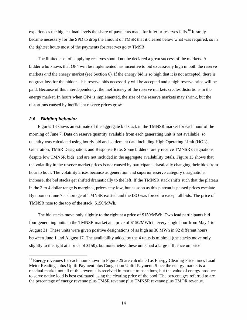
2.6 Bidding behavior Figures 13 shows an estimate of the aggregate bid stack in the TMNSR market for each hour of the

morning of June 7. Data on reserve quantity available from each generating unit is not available, so

quantity was calculated using hourly bid and settlement data including High Operating Limit (HOL),

Generation, TMSR Designation, and Response Rate. Some bidders rarely receive TMNSR designations

despite low TMNSR bids, and are not included in the aggregate availability totals. Figure 13 shows that

the volatility in the reserve market prices is not caused by participants drastically changing their bids from

hour to hour. The volatility arises because as generation and superior reserve category designations

increase, the bid stacks get shifted dramatically to the left. If the TMNSR stack shifts such that the plateau

in the 3 to 4 dollar range is marginal, prices stay low, but as soon as this plateau is passed prices escalate.

By noon on June 7 a shortage of TMNSR existed and the ISO was forced to except all bids. The price of

TMNSR rose to the top of the stack, $150/MWh.

The bid stacks move only slightly to the right at a price of $150/MWh. Two lead participants bid

four generating units in the TMNSR market at a price of $150/MWh in every single hour from May 1 to

August 31. These units were given positive designations of as high as 30 MWh in 92 different hours

between June 1 and August 17. The availability added by the 4 units is minimal (the stacks move only

slightly to the right at a price of $150), but nonetheless these units had a large influence on price

10 Energy revenues for each hour shown in Figure 25 are calculated as Energy Clearing Price times Load Meter Readings plus Uplift Payment plus Congestion Uplift Payment. Since the energy market is a residual market not all of this revenue is received in market transactions, but the value of energy produce to serve native load is best estimated using the clearing price of the pool. The percentages referred to are the percentage of energy revenue plus TMSR revenue plus TMNSR revenue plus TMOR revenue.

15

formation in many hours of June and July. Not surprisingly, both of the lead participants control other

units that bid lower prices in the TMNSR market. All of these units benefited when the price was set at

$150/MWh.

Tables 15, 16, and 17 give some indication of the bidding behavior of market participants for the

entire period of May through August. The tables focus on two issues: how often units submit zero bids

and how often units set the clearing price. To weight the frequency of these occurrences we use reserve

designations and reserve revenue. Because hourly prices are averages of five-minute prices, and because

more than one unit can submit the same bid, more than one unit can help set the clearing price in any

given hour. If a unit submitted a bid that was greater than or equal to the clearing price, and received a

positive designation, it is probable that the unit set the clearing price for at least some of the hour. The

inter-temporal optimization of the SPD causes some high bids to be accepted even though they do not

help set the clearing price, but this is relatively rare. In the majority of hours there is only one bidder with

a bid as high as the clearing price. The TMSR market was not analyzed because the ISO considers lost

opportunity cost in addition to bids to determine a clearing price. We did not have sufficient five-minute

data to analyze this market.

Tables 15 and 16 analyze bidding by type of unit. The revenue and designations earned by each

individual unit when the unit was bidding zero or bidding at least the clearing price were calculated. The

units were then grouped by unit type, and revenue and designation values aggregated together. Tables 15

and 16 show that fossil fuel burning generators tend to submit zero bids for TMNSR and TMOR whereas

hydro resources are more likely to submit high bids and set the price. Overall, 74% of all TMNSR

designations and 82% of TMOR designations from May through August were given to units that

submitted zero bids.

Table 17 shows that the largest lead participants received a large proportion of their designations and

revenues in hours that they were helping to set the price. A single lead participant can have many

different generating units, each with a different TMNSR bid price in any given hour. If any of a lead

participant’s generating units bid at least the clearing price and was given a positive designation then all

of that lead participant’s units’ TMNSR revenue for that hour was included (likewise for TMOR). For

anonymity, the bidders IDs have been renumbered and ordered from the greatest TMNSR revenue to the

least for the May – August period. Of all of the TMNSR revenue that the first TMNSR provider received,

46% was earned when the lead participant had a unit with positive designations that was bidding at least

the TMNSR price. The second TMNSR provider sets the price most often (1006 out of 2952 total hours

16

with a successful bid of at least the TMNSR price), but when it did, the price was low, so the participant

did not receive a great deal of revenue in these hours (only 5% of the participant’s total).

3 The ISO’s short-term remedies Recognizing the signs of market failure in the reserve markets, the ISO introduced two short-term

remedies.

ISO Reserve remedy: Cap the reserve prices with the energy price.

On June 27, 1999, the ISO capped the reserve prices with the energy price. Initially, this was done on

a five-minute basis. Whenever the clearing reserve price in the five-minute interval was above the five-

minute energy price, the reserve price was reduced to the greater of the energy price or 0. This was

applied to all three reserve markets (TMSR, TMNSR, and TMOR). Later, in July 1999, the ISO switched

to applying the cap on an hourly basis. Whenever the reserve price in the hour was above the hourly

energy price, the reserve price was reduced to the energy price. The shift from five-minute to one-hour

application of the cap effectively raises the cap slightly, depending on the variability of prices within the

hour.11

Despite the cap, there are several cases where the reserve prices were above energy price (see Table

12). Many of these cases are the result of a downward revision of the energy price due to an emergency

sale. If the revision occurs more than five days after the event, then the ISO does not have the power

under the rules to revise the reserve prices. The few remaining cases are simply processing errors. Only

recently has the ISO been able to automate the application of the cap. Thus, for most of the four-month

period, the cap was applied manually, and some instances where the cap should have been imposed were

missed.

The cap on reserve prices improves the original market structure, but falls far short of an efficient

solution. Consider the energy bid of a producer who is capable of supplying reserves. If the bidder knows

that there will be a scarcity of reserves and that the reserve price will be capped by the energy price then

the bidder has no incentive to submit a bid that will be successful in the energy market. If the bidder is

selected to produce energy it will be paid the energy clearing price and will incur operating costs. If the

bidder is not selected to produce energy it will be selected to provide reserves (everyone is selected when

reserves are scarce). In this case the bidder will receive the energy clearing price (the capped reserve

11 If within hour prices are fairly stable, this change has little effect; if within hour changes are large, the effective raise in the cap is large.

17

price) and will not incur operating costs. The bidder does strictly better if its energy bid is not selected

because it avoids operating costs. To ensure that it is not selected the bidder will set its bid as high as

possible. If all bidders follow this strategy a reasonable energy price cannot be produced. The gap

between the energy price and the reserve price should induce suppliers to limit their energy bids. A price

cap does not create this gap. Section 6 elaborates on the relationship between reserve prices and energy

bids.

ISO OpCap remedy: Cap the OpCap price in OP 4 conditions with five times the average of the

three highest hourly clearing prices in the previous thirty days during non-OP 4 conditions.

The cap on the OpCap price in OP 4 conditions was applied retroactively to the beginning of the

market. The cap, however, was not binding until particular days in June.

4 Options for medium-term remedies The ISO’s short-term remedies have been an essential and important step in improving the NEPOOL

markets. Both remedies involve the use of price caps. Although price caps are inconsistent with

competitive markets, their careful application in response to market design flaws is necessary. The ISO,

recognizing the dangers of rigid price caps, wisely decided on market-based price caps, allowing the cap

on reserves to vary with the energy price and allowing the OpCap cap to vary with the highest OpCap

prices in non-emergency situations. Both of these remedies should be continued until a better solution can

be implemented.

The ISO and NEPOOL should continue to work aggressively on a long-term fix to the basic design

flaws in the reserves. The recent work of NEPOOL’s Congestion Management and Multi-settlement

Committee is an important step in the right direction. However, realistically it is unlikely that the long-

term solution will be implemented until 2001, given the complexity of the issues involved. Hence, it is

important to identify a medium-term fix that the ISO can implement within a matter of months. We

present such a medium-term solution below.

Recommendation: Eliminate the OpCap market.

The market flaws in the OpCap are severe. Fortunately, there is an easy medium-term fix that is also

a long-term fix—eliminate the OpCap market. One cannot argue that the OpCap market serves any useful

purpose as presently designed. Since its operation has real costs with no apparent gain, the market should

18

be eliminated. Capacity should be rewarded in the energy and reserve markets, and not in some phony

market.12 (The ISO has taken our advice and eliminated the OpCap market as of March 1, 2000).

Recommendation: Adopt the smart buyer model for the reserve markets.

We recommend that the reserve markets continue in the medium-term, but with the ISO adopting a

smart buyer model for reserves. As a smart buyer, the ISO:

1. Never pays for additional reserves more than the economic value of the additional reserves.

2. Reduces its demand for reserves as reserve prices increase.

3. Shifts purchases toward higher quality reserves when they are priced less than lower quality

reserves.

In conducting the markets for reserves, the ISO is effectively purchasing reliability on behalf of load. The

ISO has a responsibility to purchase wisely, given the aggregate preferences of load. On this basis, the

ISO as smart buyer develops a demand curve for reserves that reflects the marginal value that additional

reserves have for the system.

The essential elements of the smart buyer model can be adopted in the medium-term. The ISO

recently has implemented point 3 above. The reserves now are treated as a cascade with the ISO filling its

need for lower quality reserves with higher quality reserves if the higher quality can be purchased at a

lower price. The difficult step is establishing a demand curve for reserves, which reflects the marginal

value of additional reserves. This will accomplish points 1. Point 2 is accomplished by integrating the

demand curve with the unit commitment and dispatch programs. It will require some discussion among

participants and regulators, but once new operating procedures are established the ISO can begin

purchasing reserves according to its demand curve, rather than the current vertical “demand” curve, which

does not reflect the marginal value of additional reserves.

The demand curve for reserves may sound like an arbitrary object. One may fear that determining the

demand curve will quickly turn into heated debates about the value of lost load. Although we anticipate

lively discussions, we believe that a reasonable approximation of the demand curve can be constructed in

an implementable way. The key is focusing on what a demand curve is. The demand curve for reserves

12 If participants want to play the “ask and it shall be given” game, they should do so on a voluntary basis. Moreover, the activity should not be orchestrated by the ISO, since it has nothing to do with running a reliable and efficient electricity market. We doubt that the game would survive such a market test.

19

specifies for every quantity of reserves the marginal value of additional reserves. Today there are tractable

methods for determining these values from the shadow prices of the appropriate optimization problem.

In what follows, we will assume that the ISO is able to construct a downward-sloping demand curve

for reserves.

Recommendation: Restructure the reserve markets.

The basic flaws in the reserve markets stem from two features of the current markets:

1. The vertical “demand” curve, derived from a rigid reserve requirement, implies that prices are

arbitrarily high in times of scarcity.

2. Losing bidders face the same obligations as winning bidders.

The first flaw is eliminated by constructing the true demand curve for reserves, based on the

marginal value of additional reserves. The second flaw can be solved in two ways.

The first way is to construct one or more forward reserve markets. Then the losing bidders would

learn that they are not needed to provide reserves, while they still have time to find something to do with

their excess supply, such as offering it in another market. This is the approach used in California and

some other markets (Chao and Wilson 1999). We do not believe that this is a feasible solution in the

medium-term. The construction of new markets cannot be done in a few months. Day-ahead reserve

markets are planned in the long run as part of the CMS/MSS Straw Proposal.

The second solution to flaw 2 is to revise the structure of the reserve markets in a way that is

consistent with the basic market features in place today. These basic features are (1) ex post clearing, and

(2) an obligation of all operable capacity to participate in the market (i.e., respond to the dispatch

instructions of the ISO). Features (1) and (2) imply that the true supply curve is in fact vertical—a fixed

supply of reserves is offered to the market regardless of price. This is illustrated in the diagram below.

The first pane illustrates the current market structure for reserves. The bidders submit offers from which

the aggregate “supply” curve (S) is formed. The ISO establishes the reserve requirement, forming the

vertical “demand” curve (D). The ISO then designates the reserves (QD) and the clearing price (P). Those

with bids below P are paid; those with bids above P are not. All available supply (QS) provides reserves in

the sense that they provide dispatch flexibility to the extent that they can respond to dispatch instructions.

Under the revised market structure illustrated in pane (b), the clearing price is found by intersecting

the true supply curve (ST), computed by the ISO based on the participants’ ability to respond to dispatch

20

instructions, and the true demand curve, computed by the ISO from its dispatch and ancillary

optimizations. The result is the price (PT), which is received by every participant that is providing needed

dispatch flexibility.

Price

P

S D

QD Quantity

(a) Current Market Structure for Reserves

Price

PT

DT

ST

QS Quantity

(b) Revised Market Structure for Reserves

QS

The revised market structure replaces the flawed markets for reserves with markets based on sound

economic principals.

5 The marginal value of reserves A demand curve is a useful conceptual tool, but slightly misleading. What we envision is a demand

function, which maps system conditions to a vector of three reserve prices. For example, the TMSR price

will be decreasing in the amount of TMSR available (as demonstrated by drawing a downward-sloping

demand for TMSR), but it will also be decreasing in the amount of TMNSR and TMOR available. When

a single function is used to produce all three prices there is no need for a sequential clearing of markets.

The function should be derived so that it sets prices that increase with the quality of the reserve. The

TMSR price will be at least the TMNSR price which will be at least the TMOR price.

5.1 Estimating the marginal value of reserves The purpose of the reserve markets must be identified before any technique for the estimation of

marginal value can be determined. Ideally real time reserves should be used solely to protect the

reliability of the system in the event of generator forced outages (Hirst and Kirby 1998). However, in

New England the lack of day-ahead markets for operating reserves shifts some of the burden of protecting

against load-forecast errors to the real time reserves. An estimation of the true marginal value of

21

additional reserves must include the contribution to bulk-power reliability as well as the commercial value

added by the additional system capacity.

Significant theoretical work has been done on the valuation of scheduled reserve capacity,

particularly for spinning reserve. Sufficient scheduled reserve capacity can correct for load forecasting

errors and generator outages without load shedding. The value of reserves can be calculated as the value

of the expected load that would have been shed if reserves were not available. It should be pointed out

that the engineering literature has focused on scheduled reserves, not reserves that are designated in real

time. Scheduled reserves can be thought of as call options. There is some positive probability that the

system operator will exercise the option and use the reserve for energy in real time. When reserves are

designated in real time there is zero probability that the reserve is used for energy; a unit is designated as

providing reserves or energy, not both. From the perspective of real time the relevant uncertainty

pertaining to reserves is the possibility of a contingency arising in the short-term future.

5.2 The model for summer 2000 We have worked with the staff of ISO New England to develop a model for the valuation of real time

reserves. The model does not produce full demand curves. Given the reserves available it finds the

marginal value of one additional hypothetical unit of reserves. This marginal value represents the height

of the demand curve at its intersection with supply. Hypothetical units of TMSR, TMNSR, and TMOR

are valued, producing three reserve prices, which descend with the quality of the reserve service provided.

The ISO plans to use the model for settlement in the summer of 2000, and may eventually adjust the

model to integrate with dispatch operations and forward markets. A brief overview of the model is

presented here. Further documentation of the model is available on the ISO’s website.13

The two distinct uses of reserves are identified and valued. First, the existence of reserves allows the

system operator to respond to contingencies without shedding load. One more MW of reserves means that

one less MW of load will have to be shed if a sufficiently large contingency arises. Ten-Minute Spinning

Reserve (TMSR), Ten-Minute Non-Spinning Reserve (TMNSR), and Thirty-Minute Operating Reserve

(TMOR) all contribute to this function. The second component of marginal value is added to the TMSR

and TMNSR price to reflect their ability to protect the stability of the system from unexpected

contingencies over a ten-minute time horizon. It may not be possible to shed sufficient load on short

notice to restore interchange with the rest of the interconnection in the required time. If this is true then

13 http://www.iso-ne.com/

22

TMSR and TMNSR do not merely save load shedding, they also may prevent cascading failure of

transmission lines, and the NERC and NPCC penalties that come with violating tie-line constraints.

The model recognizes that the reliability of the electrical system, and the effect of the addition of a

unit of reserves on that reliability, is highly dependent on the current state of the system. To derive an

accurate estimation of the marginal value of reserves the current state of the system must be described

with precision. Data that is needed to model the system includes:

1) Failure and duration rates of each generating unit

2) Capacity of each generating unit

3) Dispatch status of each generating unit (how much energy and/or reserve the unit is currently

providing)

4) Response Rate of each generating units

5) Start up times of rapid start units and hot reserve units

6) The realizations of load (ex post realizations can be used as a proxy for short term forecasts)

7) The amount of load which can be shed within ten minutes

The model uses the inputs above and standard statistical techniques to form a Capacity Outage Probability

Table (Gooi et al. 1998, Billinton and Allan 1996) for each of a series of lead times. The table describes

the probability of suffering each of a series of possible MW outages at some time in the future.

5.2.1 The first component of marginal value – value of energy saved The expected amount of energy saved by the addition of a marginal reserve unit is calculated as

difference between Expected Energy Not Supplied without considering the reserve unit and Expected

Energy Not Supplied with the reserve unit considered. Expected Energy Not Supplied is calculated using

the expected load shed at each moment of time in an interval spanning from the present to the final lead

time. The final lead time is chosen as the time it takes for sufficient capacity to become available so that

any contingency that may occur at the present moment will be covered. This time may be the start up time

of a cold reserve unit, or approximately 4 hours. For this part of the estimation of marginal value it is

assumed that load is shed whenever there is a capacity shortage. If load exceeds capacity the difference

23

between the two (the shortage) is shed.14 Both load and capacity are random variables. Uncertainty in load

is evaluated using historical data on the accuracy of the ISO’s forecasts. Uncertainty in capacity is

evaluated using the Capacity Outage Probability Table. For each of a series of lead times, the model

predicts the probability of each of a series of potential capacity shortages. A weighted sum of these

potential shortages gives the expected shortage for the lead time. The Expected Energy Not Supplied is

found as the integral of expected shortage over all lead times from the present until the final lead time.

Expected Energy Not Supplied is not of interest itself – the marginal value of reserves is the value of

one additional reserve unit. Hypothetical TMSR, TMNSR, and TMOR units are added to the model one

at a time in order to calculate the effect of each on Expected Energy Not Supplied. This drop in Expected

Energy Not Supplied is attributed to the marginal unit and is used to derive the first component of

marginal value.

(d) hypothetical TMOR unit added

(b) hypothetical TMSR unit added

(c) hypothetical TMNSR unit added

(a) no hypothetical units

Expected energy saved by hypothetical unitExpected Energy Not Supplied

expected shortage(MW)

expected shortage(MW)

lead time (minutes)10 240

lead time (minutes)24030

14 The effect of voltage reductions and other corrective actions is not considered. Because of this and other simplifying assumptions Expected Energy Not Supplied should be viewed as an index of system reliability in the short-term future, and should not necessarily be interpreted literally. Value of Lost Load should be scaled appropriately.

24

The figure above demonstrates this process (the figure is very abstract and the shapes of the curves

should not be taken literally). Expected shortage is measured by the height of the curve in pane (a).

Expected shortage is determined by two opposing forces. Expected shortage tends to rise over time

because given that a unit is operational the probability that the unit suffers an outage grows as the lead

time considered grows. Expected shortage tends to fall over time because the capacity available from

reserve units grows over time. These two forces cause the graph of expected shortage to initially rise and

eventually fall back down. The area underneath the graph of expected shortage represents the Expected

Energy Not Supplied between the present and the final lead time.

The addition of hypothetical units causes the graph of expected shortage to fall and therefore causes

a decrease in Expected Energy Not Supplied. Pane (b) shows the addition of a TMSR unit. The

hypothetical unit has an immediate impact on the expected shortage because the unit begins ramp up

immediately. Expected Energy Not Supplied falls to the lower area, and the lightly shaded area represents

the expected energy saved by the TMSR unit. Panes (c) and (d) show the addition of non-spinning reserve

units. The units only have an effect on expected shortage after the start-up time of the unit has elapsed.

Because of this and because there is a significant probability that a non-spinning reserve unit will fail to

start the expected energy saved by the non-spin units will be less then the expected energy saved by the

spin unit.

The amount that the hypothetical unit decreases Expected Energy Not Supplied is scaled

appropriately for incorporation in a price per MWh, and is multiplied by the Value of Lost Load (VOLL)

to produce the first component of marginal value. VOLL is a crucial unobservable parameter in the

valuation of reserves. Reserve prices should never exceed VOLL since load can always be shed to

produce reserves. Estimates of VOLL range from $2/kWh to $25/kWh. Surveys show that VOLL is

dependent on the duration of interruptions, the number of interruptions, the time of day, the time of year,

availability of advance warning, the location of the interruption, as well as other variable factors. If

VOLL is assumed to be constant, and is set to the average of all of its possible values, it will not precisely

reflect the true cost of shedding load at any given time (Kariuki and Allan 1996). The model that we have

developed for ISO New England does not take into account this ambiguity in the concept of VOLL. A

more sophisticated model would value outages based on their duration.

5.2.2 The second component of marginal value – ten-minute response value In the discussion above we used “expected shortage” and “expected load shed” interchangeably. This

assumes that it if there is not sufficient capacity to cover load then load will have to be shed. It is

conceivable that there may be a delay before load can be shed if an outage occurs unexpectedly. If this is

25

true then the service provided by reserves is underestimated by the value of load saved. Reserves may

enable the system operator to restore balance between production and consumption before damage is done

to transmission lines and before tie-line constraints are violated. The ten-minute response component of

the TMSR and TMNSR prices estimates this contribution to system reliability. Many of the costs of slow

recovery are incurred in other control areas and are hard to quantify. The penalties levied for violating the

constraints are designed to internalize this externality and can be used as a proxy for the true external

cost. In addition to the penalties, costs of violating constraints may include the administrative costs of

applying a punishment, the cost of public relations, and the possibility of being sued by other control

areas. All of these costs can be aggregated into a single value that defines the cost of failing to cover an

outage with sufficient reserve or load shedding within ten minutes.

An “imbalance” occurs if there is a capacity outage that exceeds the ability of the system to respond

with reserves and load shedding.15 Note that an imbalance is not the same as what we called a shortage

above. A shortage occurs if load exceeds capacity so that load must be shed. An imbalance occurs only if

load exceeds capacity by so much that load cannot be shed sufficiently. The probability of an imbalance

at a lead time of ten minutes is chosen as a basis for measuring the reserve response value because NERC

guidelines call for tie-line balance to be restored within ten minutes of a contingency.

The derivation of the second component is very similar to the derivation of the first. The model is

analyzed without any hypothetical units and the probability of an imbalance at the lead time of 10 minutes

is recorded. The model is analyzed after the addition of a hypothetical TMSR unit and the probability of

an imbalance at ten minutes is recorded. Because an imbalance is less likely to occur when more reserves

are available it must be that the addition of the hypothetical unit reduces the probability. The reduction in

the probability of an imbalance due to the addition of a hypothetical unit is appropriately scaled and is

multiplied by the cost of an imbalance to give the ten-minute response value. The TMSR ten-minute

response value will be greater than the TMNSR ten-minute response value due to the probability that the

hypothetical TMNSR unit will fail to start. A TMOR unit provides no response within ten minutes.

5.3 Reserve valuation and unit commitment Reserve valuation models can be used for more than just the determination of prices. Gooi et al.

(1998) develop a method for incorporating the estimated value of spinning reserves into a Lagrangian

Relaxation Unit Commitment program. They show that overall cost savings are achieved when the

reserve requirement is adjusted during unit commitment based on the balance of costs and benefits (see

15 Corrective actions such as voltage reductions can also be considered.

26

also Tseng et al. 1999; Guan and Luh 1996). When reserve valuation is integrated with unit commitment

or a fully functioning day-ahead market the ISO can act as a smart buyer. The ISO will be able to reduce

purchases of reserves as the cost of supplying reserves increases and will be able to shift purchases to

higher quality reserves when it is economical to do so. Critics of the ISO’s performance in the summer of

1999 claim that the unit commitment program scheduled too many units. Units were often dispatched to

their Low Operating Limits resulting in large reserve margins and low prices. If an accurate reserve

valuation model is used in unit commitment excess scheduling can be avoided.

6 Reserve payments’ effect on energy bids When the ISO chooses which units to dispatch from the energy bid stack it also determines which

units are left over to provide reserves. In New England the decision to choose an inflexible unit out-of-

merit order so as to save a flexible unit for reserves is left to the discretion of the system operator. If a

demand curve representing the marginal value of reserves is introduced this dispatch decision can be

made easily within a cost (including interruption cost) minimizing framework. In order to determine

which units to dispatch the ISO must determine what is truly expressed by the generators’ energy bids.

The opportunity to earn revenue in reserve markets can have an effect on energy bids. Even in the

absence of market power a generator’s energy bid may not express its operating costs. A simple

theoretical model illustrates this.

6.1 A simple theoretical model The current reserve market structure is so fundamentally flawed that any attempt to analyze it with

formal economic theory is doomed to end in nonsensical results. The following analysis assumes that the

ISO revises the markets, as we have proposed above, and sets the reserve price to marginal value. For

simplicity we consider a single reserve market, and consider two types of generating units – units that are

capable of providing reserves and units that are incapable of providing reserves. The proposed reserve

market can be treated as a Cournot auction. Unlike most auctions there is no price component to each bid.

The quantity component of each bid is also unusual—bidders determine which units will be available for

reserves through their decisions to make capacity available and through their energy bids. Bidders do not

know with certainty what quantity of reserves they are bidding because there is uncertainty about load and

therefore uncertainty about which units will be called for generation. The choices that define the reserve

bid are identical to the choices that define the energy bid, so inefficient pricing in the reserve market will

result in inefficiencies in the energy market.

27

Capacity availability decisions and energy bids are set day-ahead. The energy bid for each generating

unit consists of a non-decreasing schedule of prices and quantities.16 The ISO aggregates all day-ahead

energy bids to produce a supply function, S(p), which represents the total capacity bid at less than the

price p. Since the ISO stacks bids from lowest to highest, S(p) must be a nondecreasing function. S(p) can

be expressed as the sum of two function: S(p) = S1(p) + S2(p) where S1(p) represents the aggregate supply

function of units that are capable of supplying reserves (and eligible for reserve payments) and S2(p)

represents the aggregate supply function of units that are incapable of supplying reserves. In real time the

random variable Q, representing load, is realized and an energy spot price, P, is determined such that S(P)

= Q. For now we assume that the ISO does not consider a unit’s reserve eligibility when it decides which

units will produce energy, it simply takes the energy bid stack as given and follows the merit order. Units

that bid below the energy clearing price produce energy and are paid the uniform energy price. Units that

bid above the energy clearing price produce nothing and receive the reserve clearing price if they are

eligible.

All unused capacity of reserve capable units is assumed available for reserves. Call this unused

capacity K where K = S1(∞) - S1(P). The reserve price is determined by the function R(Q, K). For

simplicity we assume that R does not depend on response rates, the inherent reliability of specific units,

or more complicated system effects. The functional form of R is determined by the ISO before the

opening of the market and is known by all participants. In this section of the paper we do not attempt to

explain how the ISO sets R; we take R as given and use it to predict bidder behavior. Assume that R is

continuous and differentiable in both arguments and strictly increasing in Q and strictly decreasing in K.

Let F(Q) be the probability that load falls below the value Q from the perspective of one day in

advance. Call the lowest and highest possible load levels Q and Q so F( Q ) = 0 and

F( Q ) = 1. Assume that F has a positive density, f, for all values of load between Q and Q .

Some simplifying assumptions allow us to address bidding behavior. We consider all bidders to be

small compared to the size of the overall market so that bidders do not actively attempt to game the

energy price or the reserve price. This assumption allows us to consider the bid of each generating unit

independently. Furthermore assume that the costs of generating units are heterogeneous and dispersed

16 Typically energy bid schedules are restricted to a finite number of steps. No such restriction is made here.

28

such that S(p) is continuous and ( )S p′ exists and is positive for all quantity values between Q and Q .17

These assumptions guarantee that there is a unique solution to S(P) = Q and therefore a unique clearing

price. This market clearing equation can be inverted to give the functional relationship defining the

energy clearing price for every realization of load, P = P(Q).

Consider the problem of a reserve capable supplier who has already decided to make its unit

available. The remaining choice is what bid price should be submitted. Since generating units are

assumed to be atomistic, the bid of one unit does not affect the probability that another unit will be called

for generation, and does not affect either price. There is no strategic interplay between the bids of a

supplier, so we can consider all of the supplier’s generating units and each megawatt of capacity within

each of the supplier’s units independently. Assume that the operating cost of the bidder is such that there

is some chance that the bidder will be the marginal bidder.

The real time payoff (ignoring availability costs) per MWh for an increment of capacity with

marginal cost, c, can be expressed in terms of its bid b:

( )1

( )( , ) ( , ) ( ) ( ( ) ) ( )

S b Q

Q S bb c R Q K f Q dQ P Q c f Q dQπ = + −∫ ∫ .

If the realization of load is below S(b) the reserve price is paid; if the realization of load is above S(b) the

energy price is paid and the operating cost is incurred. Maximization of this real time payoff with respect

to b yields the first order condition:

( ) ( ( ))[ ( ( ), ) ( ( )) ] 0S b f S b R S b K P S b c′ − + = .

This can be simplified to give the expression defining the optimal choice of b (assuming the second order

condition holds), denoted b*:

1) * ( ( *), )b R S b K c= + .

Bidders who can supply reserves forecast what the reserve price would be if their bid was the marginal

bid in the energy market and add this value to marginal cost to produce their bid. This inflation of the bid

17 A sufficiently generous reserve price function will ensure that there is enough supply to satisfy even the highest load contingency Q . If we assume that R is set such that S(∞) is strictly greater than Q then we do not have to worry about the existence of a supplier who knows that his bid will necessarily be accepted in some states of the world. The entry of a surplus of suppliers can only be rationalized if the excess suppliers have zero availability cost. These suppliers can be thought of as dispatchable load.

29

above marginal cost is not an attempt to push up the energy price, it is merely an inclusion of all costs of

being selected to produce energy—the operating cost and the opportunity cost of lost reserve revenue.

There is no opportunity cost for a bidder who is ineligible for reserve payments, so reserve ineligible

bidders bid their operating cost only.

If all reserve eligible bidders follow the optimal bidding strategy given in equation 1), then the

marginal reserve eligible bidder18, i.e. the bidder who sets the energy clearing price, bids exactly the

reserve price above its marginal cost. If C1(q) represents the marginal cost of the unit in the reserve

capable bid stack that has q MWs of cheaper reserve capable capacity below it (the aggregate marginal

cost function of reserve capable units) and C2(q) represents the marginal cost of the unit in the reserve

incapable bid stack that has q MWs of cheaper reserve incapable capacity below it (the aggregate

marginal cost function of reserve incapable units) then we can express the inverse supply function as19

2) P(Q) = R(Q, K) + C1(S1(P(Q))) or

3) P(Q) = C2(S2(P(Q))).

Differentiation of equation 2) with respect to Q yields

1

1 2( ) ( , ) ( , ) dK dCP Q R Q K R Q KdQ dQ

′ = + + , where

1

0dK dS dPdQ dP dQ

= − < and

1 1 1

0dC dC dS dPdQ dq dP dQ

= >

18 The assumption that both S1(p) and S2(p) are continuous implies that the last reserve capable unit accepted and the last reserve incapable unit accepted both bid the same amount – the clearing price. Both of these bidders can claim to be the marginal unit. 19 This expression assumes that when the realization of load is Q, the MW that sets the energy price is the one with Q units of cheaper capacity. This assumption is verified when it is shown that bids are increasing in cost.

30

No matter how the ISO sets the reserve price function, energy suppliers always bid so that the energy

price is more sensitive to an increase in the realization of load than the reserve price is. 20 This result

implies that the second order condition always holds.21

Total differentiation of the bid optimality condition gives

1

1 2

11

2

* 1 11 ( ( *), ) ( *)

dK dCR Rdb dQ dQ

dK dCdc R S b K S b RdQ dQ

+ += = ≥

′− +.

Bids of reserve eligible units increase with marginal cost. The bids of units that are unable to supply

reserves also increase with cost. This guarantees that the lowest operating cost units of each type are

selected to produce energy. However, since each reserve eligible unit adds an opportunity cost to its bid

some reserve ineligible units will be called to produce energy even though they have higher operating

costs then some units that are left for reserves. The operating cost component puts the reserve eligible

units relatively high in the energy stack.

6.2 Efficiency Implications The efficiency in the dispatch of units based on the bidding behavior solved for above is dependent

on the accuracy of the reserve price function. If the reserve price function is set as an accurate

representation of the marginal value of reserves then the opportunity cost added to a unit’s energy bid

reflects the cost to society of the unit being unavailable for reserves. Economic efficiency demands that

this cost be considered in the dispatch of units. The placement of units that are available for reserves

relatively high in the merit order is desirable. A system operator should be more reluctant to dispatch the

flexible units because in doing so the reserve margin is decreased.

Consider the problem of a social planner who chooses which units to dispatch in order to minimize

the sum of operating costs and interruption costs subject to the load requirement. Assume that the reserve

20 If R is differentiable with respect to Q and K and strictly increasing in Q then the earlier assumption that ( )S p′ exists and is positive holds.

21 The second order condition can be expressed 1( *) ( ( *))[ ( *) ( ( *), ) 1] 0S b f S b S b R S b K′ ′ − ≤ . This can

be rearranged to give 11( ( *), ) ( ( *))( *)

R S b K P S bS b

′≤ =′

31

price function accurately describes the marginal interruption costs avoided. Let 1S and 2S represent the

energy supplied by reserve capable and reserve incapable units respectively. Let 1S and 2S represent the

total capacity available from the two types of units. Assume that the total capacity available from each

type of unit is sufficiently large so that the constraints 1 1S S≥ and 2 2S S≥ do not bind. After observing

the realization of load the social planner’s problem can be expressed as

1 2 1 1

1 2

1 2

, 0 0 0

min ( ) ( ) ( , )S S S S

S SC q dq C q dq R Q k dk

−

+ −∫ ∫ ∫

subject to

1 2S S Q+ =

If λ is used as a Lagrange multiplier then the first order conditions of the constrained optimization

problem are

4) 1 1 1 1( ) ( , ) 0C S R Q S S λ+ − − = and

5) 2 2( ) 0C S λ− =

Along with the constraint, these first-order conditions define the optimal quantity choices. Equations 4)

and 5) are identical to equations 2) and 3) with the shadow price λ taking the place of the energy clearing

price and the efficient quantity choices of the social planner taking the place of the decentralized

equilibrium of the auction. Therefore, the auction achieves the efficient dispatch of units that are made

available.

The intuition behind these results can be seen with a simple example. Consider two units with equal

generating capacity. Unit A is eligible to receive the reserve payment, and unit B is ineligible. Unit A has

operating costs of $25/MWh and unit B has operating costs of $30/MWh. For simplicity assume that the

reserve price function takes the constant value of $10/MWh. The above analysis shows that if the bidders

have no market power then unit A will bid at $35/MWh and unit B will bid at $30/MWh. If load is

realized such that the energy clearing price is $32/MWh then unit B will be dispatched for energy and

make operating profits of $2/MWh while unit A will receive the reserve payment of $10/MWh and incur

no operating costs. Dispatching unit B instead of unit A is efficient even though unit A has lower

operating costs. Including unit A in the dispatch instead of unit B would save $5/MWh in operating costs,

but would sacrifice $10/MWh in reserve value.

32

As long as reserves are priced efficiently a system operator need only consider energy bids to

achieve an efficient dispatch. If units A and B were forced to bid their operating costs a smart system

operator would recognize the social cost involved with the dispatch of A and would choose to dispatch

unit B out of merit order so as to save A for reserves. By allowing A and B to bid freely the system

operator can stick to the merit order22 since A has already incorporated all social costs in its bid.

It should be noted that the inclusion of opportunity costs in energy bids is not unique to the proposed

market. Any auction where winning eliminates profitable opportunities will result in this same type of

bidding. If instead of automatically giving suppliers reserve designations the ISO forces suppliers to bid

for them, there is still a loss of expected reserve revenue when a unit is called for generation. Theory

predicts that this opportunity cost must be added to the unit’s energy bid. If reserve markets are settled

day-ahead, as they are in California, bidders in the day-ahead energy market will incorporate the profit

opportunities available in the reserve markets (and real time energy market) in an opportunity cost

component of their bid.

System operators may be skeptical about encouraging reserve eligible bidders to include the

opportunity cost of lost reserve payments in their energy bids. The reserve price should be very

significant in times of scarcity, and bids significantly above operating cost are viewed with suspicion.

Also, the market presented above does not take advantage of the ISO’s informational advantage. Bidders

must predict what the reserve price would be if they were the marginal unit - the ISO knows the actual

realized value.

A revision of the dispatch rule induces bidders to submit operating costs and maintains the efficient

dispatch. The system operator tells bidders that the reserve price (marginal value of reserves) will be

added to their bid when the bid is considered in the energy stack. This eliminates the need for reserve

eligible bidders to include an opportunity cost component in their bid – the system operator does it for

them. If a reserve eligible bidder bids its operating cost they are dispatched if and only if the energy

clearing price exceeds their operating cost by at least the reserve price. Units provide reserves when the

reserve price exceeds their potential operating profit, and produce energy when their operating profit

exceeds the reserve price. It is a weakly dominant strategy for all bidders to bid their operating cost. The

dispatch is identical to the dispatch presented above and is efficient.

If the reserve price function does not accurately represent the marginal value of reserves then the

opportunity cost component of a unit’s energy bid does not accurately represent the social cost of

22 The merit order may not be followed due to intertemporal optimization.

33

including the unit in the energy dispatch. Arbitrary reserve pricing, as in New England’s current market

structure, will lead to arbitrary energy pricing, even in the absence of market power.

6.3 The Availability Decision To analyze the availability decision, consider units with one MW capacity and constant marginal

cost. The cost of making a unit available, including labor costs, start-up costs, and opportunity costs, must

also be considered. Let the availability cost of a reserve eligible unit with marginal cost c be 1( )cσ . Let

the availability cost of a reserve ineligible unit with marginal cost c be 2 ( )cσ . Units with high operating

cost have little opportunity for profit outside the market of interest, so they have low opportunity cost of

making capacity available. Therefore,1d

dcσ and

2ddcσ are assumed to be negative.

A unit enters the market if the payoff from entering exceeds the availability cost. The entry

conditions for reserve eligible and ineligible units are:

6) ( *) 1

( *)( , ) ( ) ( ( ) ) ( ) ( )

S b Q

Q S bR Q K f Q dQ P Q c f Q dQ cσ+ − ≥∫ ∫ , and

7) 2

( *)( ( ) ) ( ) ( )

Q

S bP Q c f Q dQ cσ− ≥∫ .

Equations 6) and 7) define the set of units that enter the market (the ISO’s role in unit commitment is

ignored). Both sides of the inequalities are decreasing in c, so it is possible that low marginal cost units

enter, high marginal cost units enter, or a mixture of both enter.

An alternative way to state the entry condition is a supplier makes its capacity available as long as

expected cost does not exceed expected revenue. Equations 6) and 7) can be rewritten as

( *)1 1 1

0 ( *)E(cost )= ( ) (1 ( ( *))) ( , ) ( ) ( ) ( ) E(revenue )

S b Q

S bc F S b c R Q K f Q dQ P Q f Q dQσ + − ≤ + =∫ ∫ , and

2 2 2

( *)E(cost )= ( ) (1 ( ( *))) ( ) ( ) E(revenue )

Q

S bc F S b c P Q f Q dQσ + − ≤ =∫

Expected cost can be increasing or decreasing in c, but expected revenue is strictly decreasing in c.

1E(revenue ) * *( *) ( ( *))[ ( ( *)) *] ( *) ( ( *)) 0d db dbS b f S b R S b b cS b f S bdc dc dc

′ ′= − = − < , or

34

2E(revenue ) ( *) ( ( *)) * 0d S b f S b bdc

′= − < .

Low operating cost units provide energy more often than high operating cost units because they place

themselves lower in the stack. Because the energy price exceeds the reserve price (by marginal cost), the

low cost units receive more expected revenue.

This result may lead to inefficient availability decisions. The entry of a unit with low availability cost

and high marginal cost may reduce the total cost of supplying load by the same amount as the entry of a

unit with high availability cost and low marginal cost, but the high marginal cost unit is less likely to

enter since it has lower expected revenue. This inefficiency arises because the energy market is run in real

time and availability costs are sunk when the market clears. This does not depend on the method used to

set the reserve price. Suppliers include availability costs in their energy bids only if energy schedules are

set one day in advance.

6.4 Market Power Four major results follow from the above discussion.

1. Bidders take into account the opportunity cost of foregone reserve revenue when making their

energy bids.

2. Bids of units that are eligible for reserve payments increase with operating cost. If all units are

eligible to supply reserves then low cost units are called for energy before high cost units. If only

some units are eligible for the reserve payment the units capable of supplying reserves will place

themselves relatively high in the energy stack and will be called for energy relatively infrequently.

3. Regardless of how sensitive the reserve price function is to the realization of load, bidders submit

an aggregate supply schedule that makes the energy price more sensitive to the realization of load.

4. Even if the reserve price is set accurately availability decisions may not be efficient.

It is useful to consider how the theoretical results would be effected if the model was extended to

include the existence of market power. From May through August 1999 in New England, two lead

participants earned 47% of the energy revenue, 65% of the TMSR revenue, 58% of the TMNSR revenue,

and 60% of the TMOR revenue. It is hard to argue that these lead participants have no price setting

ability.

If generating units are not atomistic then the bid of one unit affects the payoff function of other units.

The capacity increments of a single supplier cannot be analyzed independently because all of the

35

supplier’s bids must be optimized simultaneously. A framework similar to the one presented by

Klemperer and Meyer (1989) can be used to analyze the behavior of bidders when their strategy space is a

schedule of prices and quantities. A unique equilibrium cannot be found in this environment (when the

support of load is bounded), but Klemperer and Meyer show that in any equilibrium where all participants

submit upward sloping supply functions, bids by all participants at all quantity levels are at least marginal

cost.23 When there is a real time reserve market to fall back on this marginal cost must include operating

cost and opportunity cost. In the presence of market power, an energy bid will be at least marginal

operating cost plus the reserve price conditional on that bid being the marginal bid. Therefore the energy

price will exceed the marginal operating cost of the last reserve capable unit scheduled by at least the

reserve price.

When suppliers are asymmetric, the burden of lifting price above marginal cost falls

disproportionately on the largest bidders.24 A bidder with small capacity will bid close to marginal cost

since its probability of setting the clearing price is low. A larger bidder with many units will be more

willing to inflate bids above marginal cost because the probability that one of the bids set the price is

greater, and when a bid does push up the price all of the bidder’s accepted capacity benefits. This

imbalance can lead to an inefficient dispatch of available units. Units owned by large bidders will be

placed inefficiently high in the merit order because of their inflated bids.

Market power may result in additional distortions in availability decisions. In order for the reserve

price to reflect the tightness of the market it must be decreasing in the amount of capacity available. This

relationship results in a perverse incentive for a supplier with market power to withhold capacity in order

to drive up the reserve price. This is perhaps the most compelling criticism of the real time reserve market

and the best argument for why forward reserve markets should eventually be implemented. A similar

problem was created by the market rules in England and Wales.

6.5 Lessons from the English experience The central energy market in England and Wales, known as the pool, has used capacity charges and

availability payments since its inception. These payments are determined day-ahead based on expected

reserve margins and so are fundamentally different from what is proposed here. However, these payments

23 If marginal costs are upward sloping then only the lowest quantity increment and the highest quantity increment of any supplier can be bid at marginal cost. All other quantity will be bid strictly above marginal cost. 24 This is a general result of uniform price auctions and has nothing to do with the reserve payment.

36

demonstrate the potential problems that arise when payments are made to suppliers based on the total

availability of reserves.

The capacity charge is part of the day-ahead pool purchase price and is paid per MWh of load

served. The charge is calculated by subtracting the System Marginal Price (the price that clears the energy

bid stack) from the estimated value of lost load (VOLL) and then multiplying by the loss of load

probability (LOLP). VOLL was originally set at £2 per kWh and has increased annually. The LOLP is

calculated for each half hour period of the coming day using conventional probability theory, and is a

decreasing function of the expected amount of excess capacity available. Generators that have capacity

available but not actually used receive the availability payment. A unit’s payment is calculated by

subtracting the higher of the System Marginal Price and the unit’s bid price from VOLL and multiplying

this by LOLP.

The capacity charge and availability payment were designed to reward suppliers who were available

when high load or generator outages cause the system to become tight. Economists criticized these market

rules because suppliers can determine when the system becomes tight by strategically timing planned

outages. Since LOLP increases as expected excess capacity decreases generators are able to gain large

payments by withholding capacity. Bunn and Larsen (1992) show that the extreme convexity of LOLP at

low levels of the expected reserve margin makes the incentive to withhold capacity especially strong

when the expected reserve margin is low and the system is most vulnerable. Wolak and Patrick (1998)

demonstrate that the two largest participants in the pool tend to reduce their availability below the levels

that would be predicted by NERC average availability factors, and tend to reduce availability more often

than other participants. This behavior is consistent with strategic capacity withholding because it is the

largest participants that have the most to gain from reducing their availability. Wolak and Patrick also

find that capacity withholding leads to low reserve margins even in hours where the System Load is

relatively low.

Like the English rules, the proposed revisions to New England’s reserve markets pay high amounts

when availability is low. It is crucial that the markets be designed so that availability is not made low

strategically in order to force high payments. We believe this is possible for the following reasons:

1. The proposed rules do not involve anything analogous to the English capacity charge. Suppliers of

energy are rewarded with high prices in peak hours because the market clears far up the energy

bid stack. There is no reason to add an ad hoc payment to the energy price reflecting the tightness

of the reserve markets. As we have shown above, even in the absence of market power, rational

bidding strategies will cause the energy price to rise as the reserve price rises. The incentive to

37

withhold capacity is obviously much less when the reserve margin only directly effects payments

made to units providing reserves. Since reserve totals are a small fraction of energy produced,

doing away with the capacity charge does away with much of the incentive to withhold capacity.

2. Market power in England and Wales was more of a problem than in New England. Deregulation

in England and Wales resulted in only two firms that regularly set the price. In New England the

two largest Lead Participants account for approximately half of the capability and slightly more

than half of the revenue in the reserve markets.

3. Demand curves can be derived with sufficient elasticity so that a reduction in availability does not

lead to an excessive price increase. Wolak and Patrick make a similar observation about the

English market:

The true value of the VOLL to consumers and the true relationship between the estimated reserve margin and LOLP are unknown to the regulator, but the magnitude of VOLL or the function specified to relate the expected reserve margin to the LOLP can have a tremendous impact on the observed market clearing prices. For example, setting the VOLL too high can make the payoff from strategic capacity choice timed with demand fluctuations during days and across the year a profitable strategy. If the relationship between the LOLP and the expected reserve margin is too steep in absolute value, this can also increase the profitability of this strategy. Consequently, the regulator overseeing the operation of the pool should view such variables as the VOLL and the function relating the reserve margin to the LOLP as instruments for obtaining the desired market outcomes, rather than as fixed constants or relationships.

The ISO should not be constrained to choosing demand curves that reflect the marginal benefits

of additional reserves precisely. If the marginal value is calculated to be very steep over a range

of reserve levels, a mechanism can be used to flatten out the demand curve in that range. For

example, the algorithm used to derive demand curves can be constrained to keep the demand

curves above a specified elasticity.

4. A well-defined algorithm for determining each demand curve should be implemented, and its form

communicated to all participants, but the ISO must retain the power to adjust the parameters and

methodology of the algorithm in response to market performance. It is important that suppliers of

reserves understand the market structure in order to participate efficiently, however, this should

not constrain the ISO’s ability to make quick and decisive corrections. Corrections of the market

flaws in England and Wales have been slow in coming.

7 The reserve markets in the long-term For the reserve markets to be efficient, it will be necessary to create one or more forward reserve

markets. Then the losing bidders would learn that they are not needed to provide reserves, while they still

38

have time to find something to do with their excess supply, such as offering it in another market. Chao

and Wilson (1999) describe one approach, which has been adopted in California. Although construction

of a new market cannot occur in a few months, the ISO and NEPOOL participants should continue their

efforts toward a long-term solution of the reserve markets.

The development of a long-term solution is beyond the scope of this paper. However, we will

comment briefly on the design effort to date. The CMS/MSS Straw Proposal of November 1999 presents

a multi-settlement proposal for reserves. In the day-ahead market, reserves are scheduled and generators

make financial commitments to provide reserves. The real time market serves a balancing function.

Deviations from the day-ahead commitments are settled at the real time prices. The real time reserve

markets are structured just as we have described here. The smart buyer model is employed both day-

ahead and in real time. Thus, the CMS/MSS Straw Proposal is fully consistent with all of the

recommendations made here. This will greatly ease the transition from the medium-term to long-term. In

addition, the costs to implement the medium-term recommendations are easily justified, since all the tasks

are required to implement the long run solution. In this sense, the medium-term solution is a natural step

toward the long-run solution.

One issue that has not yet been addressed in the reserve market discussions is the idea of decremental

reserves. At times, the balancing problem is that there is too much generation. The reserve market should

provide downward as well as upward flexibility. Doing so may have a positive impact in the market for

incremental reserves. One of the major problems of the real time reserve markets is that they are

inherently thin. One way to mitigate this problem is to rely more on forward markets. Another way is to

allow for greater arbitrage opportunities between energy and reserve markets. By including all four

combinations of demand/supply and incremental/decremental bids in the energy and reserve markets, new

arbitrage possibilities will be created in these markets. As a result, the reserve markets will be more liquid

and less prone to insufficient bids.

8 Conclusion The OpCap and reserve markets have serious flaws that must be addressed. The ISO’s short-term

fixes have been necessary and effective at addressing the immediate problems. However, better solutions

can be adopted in the medium term. In particular, we recommend:

1. Eliminate the OpCap market.

2. Establish a downward sloping demand curve for reserves. The demand curve would be capped in real

time by the energy price or zero, whichever is larger.

39

3. Establish the true real-time supply curve as simply the quantity of the resource made available in real

time.

4. Pay the clearing price to all resources that provide the service.

5. Never set a price in the TMSR market less than the largest lost opportunity cost.

All of these changes are consistent with the CMS/MSS Straw Proposal. These changes represent an

important step toward the long-term solution involving multi-settlement energy and reserve markets.

These markets should be designed carefully to address the basic economic and engineering issues

necessary for an efficient wholesale electricity market.

Appendix: Overview of the markets ISO New England conducts seven interdependent markets in its operation of NEPOOL’s wholesale

electricity market: (1) the energy market, (2-5) four markets for ancillary services, and (6-7) two capacity

markets. A description of each is given below. For brevity, many important details are omitted.

1. The energy market is a residual market. Only the difference between a participant’s energy resources

and its energy obligations is traded in the ISO market. These resources and obligations include

amounts covered by bilateral contracts. Hourly bids, expressed in $/MWh, are submitted on a day-

ahead basis for the next 24 hours. The ISO then schedules the generating units that will run the

following day based on minimizing total costs in the energy market, as represented by the accepted

bids. The market is settled after the fact on an hourly basis. All transactions are priced at the (ex post)

energy clearing price. Payments/receipts are equal to the MWh bought/sold times the clearing price.

Suppliers are paid for out-of-merit-order dispatch to alleviate transmission congestion on the basis of

their bids submitted in the energy market.25

2. The ten-minute spinning reserve (TMSR) market is a full requirements market. All TMSR is

bought/sold through the ISO. Bidding and settlement are done as in the energy market—hourly bids

in $/MW for the next day are submitted, and the markets are settled hourly after the fact. Given the

units dispatched to provide energy, the ISO selects the least-cost resources to provide required

TMSR, taking into account bids and lost opportunity costs. Designated resources are paid the energy

clearing price for any MWh provided. In addition, for every MW designated as spin, resources are

25 The bidder may not be paid its bid if certain transmission congestion structure and price screens are not satisfied.

40

paid the clearing price for spin, which is calculated from the bid plus lost opportunity cost. The total

cost of providing TMSR is shared proportionally by load.

3. The ten-minute non-spinning reserve (TMNSR) market is a full requirements market. All TMNSR is

bought/sold through the ISO. Bidding and settlement are done as in the energy market—hourly bids

in $/MW for the next day are submitted, and the markets are settled hourly after the fact. Designated

resources are paid the clearing price times the MW provided as reserved capacity. The total cost of

providing TMNSR is shared proportionally by load.

4. The thirty-minute operating reserve (TMOR) market is a full requirements market. All TMOR is

bought/sold through the ISO. Bidding and settlement are done as in the energy market—hourly bids

in $/MW for the next day are submitted, and the markets are settled hourly after the fact. Designated

resources are paid the clearing price times the MW provided. The total cost of providing TMOR is

shared proportionally by load.

5. The automatic generation control (AGC) market is a full requirements market. All AGC is

bought/sold through the ISO. Bidding and settlement are done as in the energy market—hourly bids

for the next day are submitted, and the markets are settled hourly after the fact. AGC is measured in

regs, which measures a unit’s ability to follow load. Units that can provide AGC at lowest cost based

on bids, lost opportunity costs, and production cost changes are selected. Generators providing AGC

are paid the clearing price for time on AGC times the number of regs plus a payment for AGC service

actually provided plus any lost opportunity cost. The total cost of providing AGC is shared

proportionally by load.

6. The operable capability (OpCap) market is a residual market. Only the difference between a

participant’s operable capability resources and its operating capability obligation (load plus operating

reserve) is traded through the ISO. Bidding and settlement are done as in the energy market—hourly

bids in $/MW for the next day are submitted, and the markets are settled hourly after the fact. A

clearing price is calculated based on the bids of those participants with excess operable capacity.

Participants who are deficient in operable capability pay the clearing price for each MW to those who

are in surplus and who bid a price less than or equal to the clearing price.

7. The installed capability market is a residual market. Only the difference between a participant’s

installed capability resources and its installed capability obligation (load plus installed operating

reserve) is traded through the ISO. Trading in this market occurs monthly. Bids are submitted in

$/MW-month on the last day before the month begins. A clearing price is calculated based on the bids

41

of those participants with excess installed capacity. Participants who are deficient in installed

capability pay the clearing price for each MW-month to those who are in surplus and who bid a price

less than or equal to the clearing price. The market is settled ex post.

References Billinton, Roy and Ronald N. Allan (1996), Reliability Evaluation of Power Systems, second edition,

Plenum Press.

Bunn, Derek W. and Erik R. Larsen (1992), “Sensitivity of Reserve Margin to Factors Influencing Investment Behaviour in the Electricity Market of England and Wales,” Energy Policy, 420-429.

Chao, Hung-po and Robert Wison (1999), “Multi-Dimensional Procurement Auctions for Power Reserves: Incentive-Compatible Evaluation and Settlement Rules,” Working Paper, Stanford University.

Cramton, Peter and Robert Wilson (1998), “A Review of ISO New England's Proposed Market Rules,” White Paper, Market Design Inc., September 1998.

Gooi, H. B., D. P. Mendes, K. R. W. Bell and D. S. Kirschen (1999), “Optimal Scheduling of Spinning Reserve,” IEEE Transactions on Power Systems, forthcoming.

Guan, X. and Peter B. Luh (1996), “Power System Scheduling with Fuzzy Reserve Requirements,” 11, 864-869.

Hirst, Eric and Brendan Kirby (1998), “Operating Reserves and Bulk-Power Reliability,” Energy, 23, 949-959.

Kariuki, K. K. and R. N. Allan (1996), “Evaluation of Reliability Worth and Value of Lost Load,” IEE Proc.-Gener. Transm. Distrib., 143, 171-180.

Klemperer, Paul D. and Margaret A. Meyer (1989), “Supply Function Equilibria in Oligopoly Under Uncertainty,” Econometrica, 57, 1243-1277.

Joint NEPOOL CMS/MSS Committee (1999), “CMS/MSS Straw Proposal,” working draft, October 14, 1999.

NEPOOL Multi-Settlement Committee (1999), “Multi-Settlement Proposal,” Final Report, March 5, 1999.

Singh, Harry and Alex Papalexopoulos (1999), “Competitive Procurement of Ancillary Services by an Independent System Operator,” IEE Transactions on Power Systems, 14, 498-504.

Tseng, Chung-Li, Shmuel S. Oren, Alva J. Svoboda and Raymond B. Johnson (1999), “Price-based Adaptive Spinning Reserve Requirements in Power System Scheduling,” Electircal Power and Energy Systems, 21, 137-145.

Wacker, Garry and Roy Billinton (1989), “Customer Cost of Electric Service Interruptions,” Proceedings of the IEEE, 77, 919-930.

Wolak, Frank A. and Robert H. Patrick (1997), “The Impact of Market Rules and Market Structure on the Price Determination Process in the England and Wales Electricity Market,” Working Paper, Stanford University.