Elements of QFT in Curved Space-Time - uni-jena.de · Indeed, for everyday life it may not be nice....

Elements of QFT in Curved Space-Time

Ilya L. Shapiro

Universidade Federal de Juiz de Fora, MG, Brazil

Theoretisch-Physikalisches Institut

Friedrich-Schiller-Universitat, Jena, February-2012

Ilya Shapiro, Lectures on curved-space QFT, February - 2012

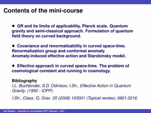
Contents of the mini-course

• GR and its limits of applicability, Planck scale. Quantumgravity and semi-classical approach. Formulation of quantumfield theory on curved background.

• Covariance and renormalizability in curved space-time.Renormalization group and conformal anomaly.Anomaly-induced effective action and Starobinsky model.

• Effective approach in curved space-time. The problem ofcosmological constant and running in cosmology.

BibliographyI.L. Buchbinder, S.D. Odintsov, I.Sh., Effective Action in QuantumGravity. (1992 - IOPP).

I.Sh., Class. Q. Grav. 25 (2008) 103001 (Topical review); 0801.0216.


Lecture 1.

GR and its limits of applicability, Planck scale.Quantum gravity and semi-classical approach.

GR and singularities.

Dimensional approach and Planck scale.

Quantum gravity and/or string theory.

Quantum Field Theory in curved space and its importance.

Formulation of classical fields in curved space.

Quantum theory with linearized parametrization of gravity.


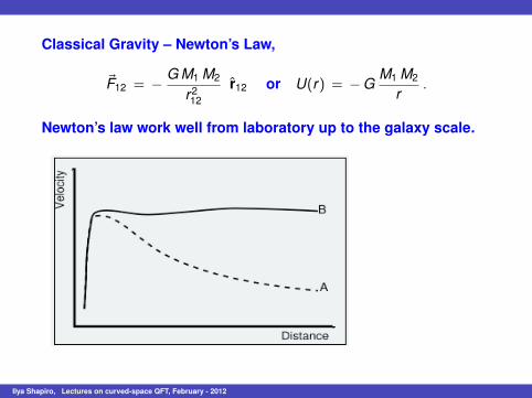
Classical Gravity – Newton’s Law,

F12 = − G M1 M2

r212

r12 or U(r) = −GM1 M2

r.

Newton’s law work well from laboratory up to the galaxy scale.


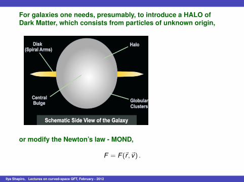
For galaxies one needs, presumably, to introduce a HALO ofDark Matter, which consists from particles of unknown origin,

or modify the Newton’s law - MOND,

F = F (r , v) .


The real need to modify Newton gravity was because it is notrelativistic while the electromagnetic theory is.

• Maxwell 1868 ... • Lorentz 1895 ... • Einstein 1905

Relativity: instead of space + time, there is a uniquespace-time M3+1 (Minkowski space). Its coordinates are

xµ = (ct , x , y , z) .

The distances (intervals) are defined as

ds2 = c2dt2 − dx2 − dy2 − dz2 .


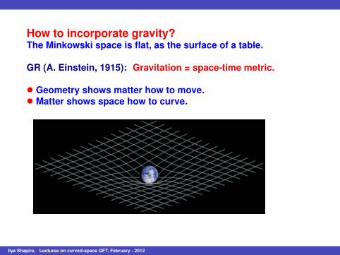
How to incorporate gravity?The Minkowski space is flat, as the surface of a table.

GR (A. Einstein, 1915): Gravitation = space-time metric.

• Geometry shows matter how to move.• Matter shows space how to curve.


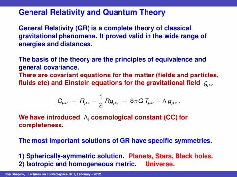
General Relativity and Quantum Theory

General Relativity (GR) is a complete theory of classicalgravitational phenomena. It proved valid in the wide range ofenergies and distances.

The basis of the theory are the principles of equivalence andgeneral covariance.There are covariant equations for the matter (fields and particles,fluids etc) and Einstein equations for the gravitational field gµν

Gµν = Rµν − 12

Rgµν = 8πG Tµν − Λgµν .

We have introduced Λ, cosmological constant (CC) forcompleteness.

The most important solutions of GR have specific symmetries.

1) Spherically-symmetric solution. Planets, Stars, Black holes.2) Isotropic and homogeneous metric. Universe.


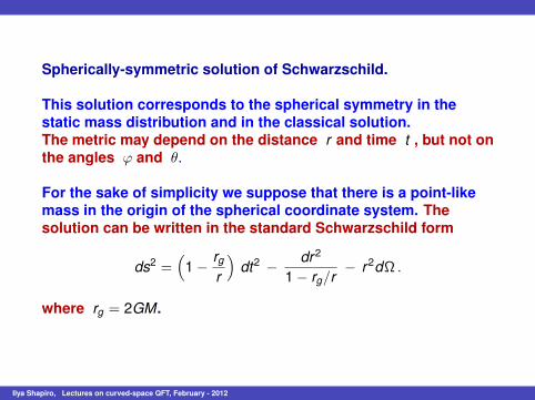
Spherically-symmetric solution of Schwarzschild.

This solution corresponds to the spherical symmetry in thestatic mass distribution and in the classical solution.The metric may depend on the distance r and time t , but not onthe angles φ and θ.

For the sake of simplicity we suppose that there is a point-likemass in the origin of the spherical coordinate system. Thesolution can be written in the standard Schwarzschild form

ds2 =(

1 −rg

r

)dt2 − dr2

1 − rg/r− r2dΩ .

where rg = 2GM.


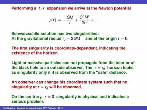
Performing a 1/r expansion we arrive at the Newton potential

φ(r) = −GMr

+G2M2

2r2 + ...

Schwarzschild solution has two singularities:At the gravitational radius rg = 2GM and at the origin r = 0.

The first singularity is coordinate-dependent, indicating theexistence of the horizon.

Light or massive particles can not propagate from the interior ofthe black hole to an outside observer. The r = rg horizon looksas singularity only if it is observed from the “safe” distance.

An observer can change his coordinate system such that nosingularity at r = rg will be observed.

On the contrary, r = 0 singularity is physical and indicates aserious problem.


Indeed, the Schwarzschild solution is valid only in the vacuumand we do not expect point-like masses to exist in the nature.The spherically symmetric solution inside the matter does nothave singularity.

However, the object with horizon may be formed as aconsequence of the gravitational collapse, leading to theformation of physical singularity at r = 0.

After all, assuming GR is valid at all scales, we arrive at thesituation when the r = 0 singularity becomes real.

Then, the matter has infinitely high density of energy, andcurvature invariants are also infinite. Our physical intuition tellsthat this is not a realistic situation.

Something must be modified.


Standard cosmological model

Another important solution of GR is the one for thehomogeneous and isotropic metric (FLRW solution).

ds2 = dt2 − a2(t) ·(

dr2

1 − kr2 + r2dΩ),

Here r is the distance from some given point in the space (forhomogeneous and isotropic space-time. The choice of this pointis not important). a(t) is the unique unknown function,

k = (0,1,−1) defines the geometry of the space section M3 ofthe 4-dimensional space-time manifold M3+1.

Consider only the case of the early universe, where the role of kand Λ is negligible and the radiation dominates over the matter.


Radiation-dominated epoch

is characterized by the dominating radiation with the relativisticrelation between energy density and pressure p = ρ/3 andTµµ = 0. Taking k = Λ = 0, we meet the Friedmann equation

a2 =8πG

3ρ0a4

0

a4 , .

Solving it, we arrive at the solution

a(t) =( 4

3· 8πGρ0a4

0

)1/4×

√t ,

This expression becomes singular at t → 0. Also, in this casethe Hubble constant

H = a/a =12t

also becomes singular, along with ρr and with components ofthe curvature tensor.

The situation is qualitatively similar to the black hole singularity.Ilya Shapiro, Lectures on curved-space QFT, February - 2012

Applicability of GR

The singularities are significant, because they emerge in themost important solutions, in the main areas of application of GR.

Extrapolating backward in time we find that the use of GR leadsto a problem, while at the late Universe GR provides a consistentbasis for cosmology and astrophysics. The most naturalresolution of the problem of singularities is to assume that

• GR is not valid at all scales.

At the very short distances and/or when the curvature becomesvery large, the gravitational phenomena must be described bysome other theory, more general than the GR.

But, due to success of GR, we expect that this unknown theorycoincides with GR at the large distance & weak field limit.

The most probable origin of the deviation from the GR arequantum effects.


Need for quantum field theory in curved space-time.

Let us use the dimensional arguments.

The expected scale of the quantum gravity effects is associatedto the Planck units of length, time and mass. The idea of Planckunits is based on the existence of the 3 fundamental constants:

c = 3 · 1010 cm/s ,

~ = 1.054 · 10−27 erg · sec ;

G = 6.67 · 10−8 cm3/sec2 g .One can use them uniquely to construct the dimensions of

length lP = G1/2 ~1/2 c−3/2 ≈ 1.4 · 10−33 cm;

time tP = G1/2 ~1/2 c−5/2 ≈ 0.7 · 10−43 sec;

mass MP = G−1/2 ~1/2 c1/2 ≈ 0.2 · 10−5g ≈ 1019 GeV .


One can use these fundamental units in a different ways.

In particle physics people use to set c = ~ = 1 and measureeverything in GeV . Indeed, for everyday life it may not be nice.

E.g., you have to schedule the meeting “just 1027 GeV−1 fromnow”, but “ 15 minutes” will be, perhaps, better appreciated.

However, in the specific area, when all quantities are (more orless) of the same order of magnitude, GeV units are useful.

One can measure Newton constant G in GeV .Then G = 1/M2

P and tP = lP = 1/MP .

Now, why do not we take MP as a universal measure foreverything? Fix MP = 1, such that G = 1. Then everything ismeasured in the powers of the Planck mass MP .

“20 grams of butter” ≡ “106 of butter”

Warning: sometimes you risk to be misunderstood !!Ilya Shapiro, Lectures on curved-space QFT, February - 2012

Status of QFT in curved space

One may suppose that the existence of the fundamental unitsindicates to the presence of some fundamental physics at thePlanck scale.

It may be Quantum Gravity, String Theory, ... We do not knowwhat it really is.

So, which concepts are certain?

Quantum Field Theory and Curved space-time definitely are.

Therefore, our first step should be to consider QFT of matterfields in curved space.

Different from quantum theory of gravity, QFT of matter fields incurved space is renormalizable and free of conceptual problems.

However, deriving many of the most relevant observables is yetan unsolved problem.


Formulation of classical fields on curved background

• We impose the principles of locality and general covariance.

• Furthermore, we require the symmetries of a given theory(specially gauge invariance) in flat space-time to hold for thetheory in curved space-time.

• It is also natural to forbid the introduction of new parameterswith the inverse-mass dimension.

These set of conditions leads to a simplest consistent quantumtheory of matter fields on the classical gravitational background.

• The form of the action of a matter field is fixed except thevalues of a few parameters which remain arbitrary.

• The procedure which we have described above, leads to theso-called non-minimal actions.


Along with the nonminimal scheme, there is a more simple,minimal one. According to it one has to replace

∂µ → ∇µ , ηµν → gµν , d4x → d4x√−g .

Below we consider the fields with spin zero (scalar), spin 1/2(Dirac spinor) and spin 1 (massless vector).

The actions for other possible types of fields (say, massivevectors or antisymmetric bµν , spin 3/2 , etc), can beconstructed using the same approach.


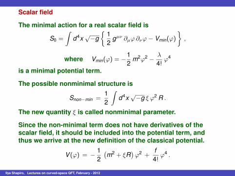
Scalar field

The minimal action for a real scalar field is

S0 =

∫d4x

√−g

12

gµν ∂µφ∂νφ− Vmin(φ)

,

where Vmin(φ) = −12

m2φ2 − λ

4!φ4

is a minimal potential term.

The possible nonminimal structure is

Snon−min =12

∫d4x

√−g ξ φ2 R .

The new quantity ξ is called nonminimal parameter.

Since the non-minimal term does not have derivatives of thescalar field, it should be included into the potential term, andthus we arrive at the new definition of the classical potential.

V (φ) = − 12

(m2 + ξR

)φ2 +

f4!φ4 .


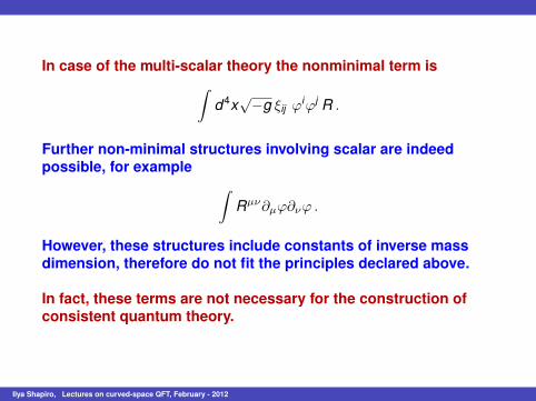
In case of the multi-scalar theory the nonminimal term is∫d4x

√−g ξij φ

iφj R .

Further non-minimal structures involving scalar are indeedpossible, for example ∫

Rµν∂µφ∂νφ .

However, these structures include constants of inverse massdimension, therefore do not fit the principles declared above.

In fact, these terms are not necessary for the construction ofconsistent quantum theory.


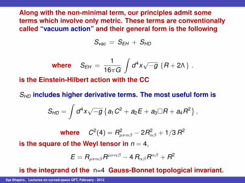
Along with the non-minimal term, our principles admit someterms which involve only metric. These terms are conventionallycalled “vacuum action” and their general form is the following

Svac = SEH + SHD

where SEH =1

16πG

∫d4x

√−g R + 2Λ .

is the Einstein-Hilbert action with the CC

SHD includes higher derivative terms. The most useful form is

SHD =

∫d4x

√−g

a1C2 + a2E + a3R + a4R2 ,

where C2(4) = R2µναβ − 2R2

αβ + 1/3 R2

is the square of the Weyl tensor in n = 4,

E = RµναβRµναβ − 4 RαβRαβ + R2

is the integrand of the n=4 Gauss-Bonnet topological invariant.Ilya Shapiro, Lectures on curved-space QFT, February - 2012

In n = 4 case some terms in the action

Svac = SEH + SHD

gain very special properties.

SHD includes a conformal invariant∫

C2 , topological and surfaceterms,

∫E and

∫R.

The last two terms do not contribute to the classical equationsof motion for the metric.

Moreover, in the FRW case∫

C2 = const and only∫

R2 isrelevant!

However, as we shall see later on, all these terms are important,for they contribute to the dynamics at the quantum level via theconformal anomaly.

The basis E ,C2,R2 is, in many respects, more useful thanR2

µναβ , R2αβ , R2, and that is why we are going to use it here.


For the Dirac spinor the minimal procedure leads to theexpression

S1/2 = i∫

d4x√

g(ψ γα ∇αψ − im ψψ

),

where γµ and ∇µ are γ-matrices and covariant derivatives of thespinor in curved space-time.

Let us define both these objects.

The definition of γµ requires the tetrad (vierbein)

eµa · eνa = gµν , ea

µ · eµb = ηab .

Now, we set γµ = eµa γ

a, where γa is usual (flat-space) γ-matrix.

The new γ -matrices satisfy Clifford algebra in curved space-time

γµγν + γνγµ = 2gµν .


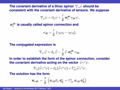
The covariant derivative of a Dirac spinor ∇αψ should beconsistent with the covariant derivative of tensors. We suppose

∇µψ = ∂µψ +i2

wabµ σab ψ ,

wabµ is usually called spinor connection and

σab =i2

(γaγb − γbγa) .

The conjugated expression is

∇µ ψ = ∂µ ψ − i2ψ wab

µ σab .

In order to establish the form of the spinor connection, considerthe covariant derivative acting on the vector ψγαψ .

∇µ(ψγαψ) = ∂µ(ψγ

αψ) + Γαµλψγλψ ,

The solution has the form

wµab =12

(eα[b∂µ eα

a] + Γαλµ eα[b eλa]

).


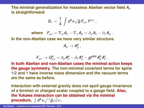
The minimal generalization for massless Abelian vector field Aµ

is straightforward

S1 =14

∫d4x

√g Fµν Fµν ,

where Fµν = ∇µAν −∇νAµ = ∂µAν − ∂νAµ .

In the non-Abelian case we have very similar structure.

Aµ → Aaµ ,

Fµν → Gaµν = ∂µAa

ν − ∂νAaµ − gf abcAb

µAcν .

In both Abelian and non-Abelian cases the minimal action keepsthe gauge symmetry. The non-minimal covariant terms for spins1/2 and 1 have inverse mass dimension and the vacuum termsare the same as before.

Interaction with external gravity does not spoil gauge invarianceof a fermion or charged scalar coupled to a gauge field. Also,the Yukawa interaction can be obtained via the minimalprocedure,

∫d4x

√−gφψψ.


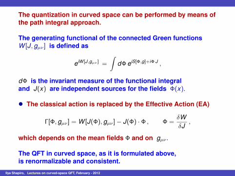
The quantization in curved space can be performed by means ofthe path integral approach.

The generating functional of the connected Green functionsW [J, gµν ] is defined as

eiW [J,gµν ] =

∫dΦ eiS[Φ,g]+iΦ J ,

dΦ is the invariant measure of the functional integraland J(x) are independent sources for the fields Φ(x).

• The classical action is replaced by the Effective Action (EA)

Γ[Φ, gµν ] = W [J(Φ), gµν ]− J(Φ) · Φ , Φ =δWδJ

,

which depends on the mean fields Φ and on gµν .

The QFT in curved space, as it is formulated above,is renormalizable and consistent.


The main difference with QFT in flat space is that in curvedspace EA depends on the background metric, Γ[Φ, gµν]

In terms of Feynman diagrams, one has to consider graphs withinternal lines of matter fields & external lines of both matter andmetric. In practice, one can consider gµν = ηµν + hµν .

→ + +

+ + + + ...


An important observation is thatall those “new” diagrams with hµν legs have superficial degreeof divergence equal or lower that the “old” flat-space diagrams.

Consider the case of scalar field which shows why thenonminimal term is necessary

→ + +

+ + + ... .


In general, the theory in curved space can be formulated asrenormalizable. One has to follow the prescription

St = Smin + Snon.min + Svac .

Renormalization involves fields and parameters like couplingsand masses, ξ and vacuum action parameters.

Introduction: Buchbinder, Odintsov & I.Sh. (1992).

Relevant diagrams for the vacuum sector

+ + + + ... .

All possible covariant counterterms have the same structure as

Svac = SEH + SHD


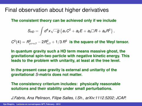
Final observation about higher derivatives

The consistent theory can be achieved only if we include

SHD =

∫d4x

√−g

a1C2 + a2E + a3R + a4R2 ,

C2(4) = R2µναβ − 2R2

αβ + 1/3 R2 is the square of the Weyl tensor.

In quantum gravity such a HD term means massive ghost, thegravitational spin-two particle with negative kinetic energy. Thisleads to the problem with unitarity, at least at the tree level.

In the present case gravity is external and unitarity of thegravitational S-matrix does not matter.

The consistency criterium includes: physically reasonablesolutions and their stability under small perturbations.

J.Fabris, Ana Pelinson, Filipe Salles, I.Sh., arXiv:1112.5202; JCAP.Ilya Shapiro, Lectures on curved-space QFT, February - 2012

Conclusions

• QFT of matter fields in curved space-time is definitely a veryimportant object of study, because it concerns real and not wellunderstood physics.

• QFT of matter fields in curved space-time can be alwaysformulated as renormalizable theory if the corresponding theoryin flat space-time is renormalizable.

• The action of QFT of matter fields in curved space-timeincludes non-minimal term in the scalar sector and additionalhigher derivative terms in the vacuum (gravity) sector.

• Different from QG, the higher derivative terms do not pose aproblem, because we do not need physical interpretation for thegravitational propagator.


Elements of QFT in Curved Space-Time - uni-jena.de · Indeed, for everyday life it may not be nice....

Documents

Transcript of Elements of QFT in Curved Space-Time - uni-jena.de · Indeed, for everyday life it may not be nice....